On boundary degrees of freedom in three dimensional Anti-de Sitter spacetime and thermofield-double

Abstract

In this article, we will study the Gibbons-Hawking-York (GHY) action over a co-dimension one hypersurface, called the “physical boundary,” close to the boundary of AdS₃. For that, we take a coordinate system that consists of two times, one is associated with evolution on the boundary, and the second is associated with evolution into the bulk. The resulting action is divergent and needs regularization. We consider two particular schemes. In the first scheme, we will add the Einstein-Hilbert on-shell action as the counter-term, which, while cancels the divergent part, adds the contribution of deep in the bulk, such as an existing horizon. The resulting action includes the Liouville action, which describes the curvature of the physical boundary. In the second scheme, however, we prescribe a natural regularization for GHY action without adding any counter-term. The resulting action will include two copies of Schwarzian actions associated with the left and right-moving reparametrization modes. At finite temperature, these modes live on two disjoint circles. We will show that these are the thermofield-double’s effective degrees of freedom. While the first scheme is more common in practice, the second scheme may be more convenient for Susskind-’t Hooft proposal for holography.

1 Introduction and Outline of the paper

The mysterious nature of an eternal black hole has offered many motivations for physicists to investigate its geometry in the past decades. While the metric can be considered one of the simplest solutions to the vacuum Einstein’s equation, it has nontrivial features. The existence of the event horizon, a co-dimension one null hypersurface where according to an outside observer, nothing can enter or escape from it, the existence of a second side in the maximal extension of the geometry, the fact that its parameters can be identified with thermodynamic quantities that satisfy the laws of thermodynamics [1], and last but not least, associating the geometry to an entangled state, namely the thermofield-double state [2] are among such features. These surprising properties have had a significant role in the development of proposals, such as the Holographic principle [3, 4], entanglement structure of spacetime [5], and ER=EPR [6].
The AdS/CFT duality [7, 8, 9] provides a systematic framework for investigating black holes. One of the consequences of the duality is that for certain “holographic theories,” correlation functions of the operators inserted on the boundary can also be computed from bulk using the AdS/CFT dictionary. While finding the exact holographic theory can be challenging, investigating the bulk puts some strong constraints on it. One of the constraints is the MSS bound [10] based on the earlier work [11, 12], which implies that the Holographic theory should satisfy the saturation of the chaos bound as the theory at finite temperature should be dual to a bifurcate horizon in the bulk.
The Sachdev-Ye-Kitaev model [13, 14, 15] is an example of a theory that meets this criterion. In its simplest form, the theory consists of a large number of Majorana fermions coupled by a random coupling. At low energy limit, the theory has an emergent reparametrization symmetry whose dynamics are effectively described by the Schwarzian action. Such modes are responsible for the saturation of the chaos bound. Moreover, the action has a geometric representation; it can be derived from the GHY boundary action in the Jackiw-Teitelboim (JT) gravity [16, 17] in the limit where the boundary of AdS2 space has small fluctuations [18]. Although the JT gravity is simple in that all of the nontrivial dynamics come from the fluctuation of the boundary, the boundary fluctuations are important in a well-defined holographic picture in higher dimensions too. The reason is as follows: the two-sided black hole is dual to the thermofield-double state [19], which can be schematically written as follows:

$$\ket{\operatorname{TFD}}\sim~{}e^{-\frac{1}{2}\beta H}~{}\sum\ket{L}\otimes\ket{R},$$ (1.1)

whose entanglement entropy equals the entropy of the black hole in the bulk. By coupling both sides and evolving the system, the entanglement entropy will change [23]. For holographic theories, the system equilibrates fast enough but with a different temperature, which can be read from the two-point function. The modes responsible for the temperature change must be generic, i.e. they should couple to all types of fields. This leads us to conjecture that, similar to the SYK/JT case, such modes must be gravitational, and to find the relevant modes, one should investigate the dynamics of the boundary fluctuations in higher dimensions. This paper attempts to do this task in AdS₃.

There have been many efforts to find a comprehensible quantum theory of gravity in three dimensions. While there is no gravitational fluctuation in three dimensional Einstein’s theory of gravity [24, 25], still the dynamics is nontrivial. It is possible to associate a central charge to the asymptotic reparametrization symmetry [26], and the theory also admits a black hole solution[27, 28]. See [29] for a review. To compute the gravitational partition function associated with the black hole in the (semi-) classical limit, one usually computes the Einstein-Hilbert action with the GHY boundary term over the possible Euclidean geometries in the bulk [30, 31]. If there is a black hole in the bulk, the integral domain of the bulk action is from the outer event horizon up to the possible boundary at infinity. This prescription naturally leads to the laws of black hole thermodynamics. In AdS₃, the boundary of the Euclidean black hole has genus one. However, adding other bulk geometries with the given boundary topology does not lead to a sensible partition function [32].

In this paper, however, we will follow a different perspective. Inspired by the idea of holography, we consider a co-dimension one time-like hypersurface called the physical boundary, embedded in asymptotic AdS₃ spacetime and “close to the boundary”(see section 2), whose dynamics are described by the Gibbons-Hawking-York (GHY) action.

$$S_{GHY}=\frac{1}{8\pi G}\int_{\partial\mathcal{M}}~{}\sqrt{-\det g_{ij}}~{}d^{2}x\Big{(}\mathcal{K}-1\Big{)},$$ (1.2)

where $\cal K$ is the trace of the extrinsic curvature of $\partial\mathcal{M}$ and $g_{ij}$ is the induced metric. In practice, we only assume that the Einstein equation is satisfied in a small neighborhood of the AdS₃ boundary. Consequently, the induced metric on the physical boundary must satisfy the momentum and Hamiltonian constraints. Under these constraints, the trace of the extrinsic curvature will take the following form:

$$\mathcal{K}=2+\frac{1}{2}r^{2}~{}^{2}\widetilde{R}^{(0)}+O(r^{3}),$$ (1.3)

where $r^{2}~{}^{2}\widetilde{R}^{(0)}$ is the curvature of the induced metric on the physical boundary. Note that this term does not lead to any dynamics, as it is accompanied by $\sqrt{-\det g_{ij}}$ of the induced metric, which is topological at conformal infinity. In fact, the nontrivial dynamics come from $\sqrt{-\det g_{ij}}$ itself. However, it is gauge dependent. A common gauge, introduced by Fefferman-Graham (FG) [33], considers the foliation of the spacetime along a spacelike direction, say $\partial_{r}$, which is everywhere normal to the leaves. AdS spacetime in this coordinate system has been studied extensively [34, 35, 36]. However, it is not considered in this paper, as it does not lead to any dynamics for the physical boundary. Instead, we will consider a different coordinate system, which is also physically more plausible for studying holography. In this coordinate system, there are two non-spacelike coordinate directions. One is the time direction, denoted by $\partial_{t}$ associated with the timelike boundary responsible for the evolution of the Hamiltonian. The second time direction, denoted by $\partial_{r}$, is responsible for the evolution in the bulk. It turns out that 1.2 leads to a nontrivial action for the physical boundary. In particular, the equations will take a simple form if we assume that $\partial_{r}$ is null. To achieve this, as opposed to the FG coordinate, we need to turn on the metric components $g_{ri}$. For simplicity, we assume that $g_{ri}$s satisfy the following general boundary conditions:

$$g_{rr}=0,~{}~{}~{}~{}~{}~{}g_{ru}=-\frac{e^{\varphi_{1}(u,v)}}{2r^{2}},~{}~{}~{}~{}~{}~{}~{}g_{rv}=-\frac{e^{\varphi_{2}(u,v)}}{2r^{2}},$$ (1.4)

to all order in perturbation.

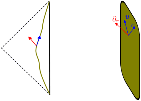
Figure 1:

Einstein equation implies that (see Appendix A):

$$g_{ij}(r,u,v)=\frac{h^{(2)}_{ij}(u,v)}{r^{2}}+\frac{h^{(1)}_{ij}(u,v)}{r}+h^{(0)}_{ij}.$$ (1.5)

On the physical boundary, the GHY action takes the following simple form:

$$S_{GHY} =\frac{1}{8\pi G}\int dudv~{}\sqrt{-\det g_{ij}}~{}+~{}S_{\textbf{top.}},$$ (1.6)

$$S_{\textbf{top.}} =\frac{1}{16\pi G}~{}\int~{}dudv~{}\sqrt{-\det\widetilde{g}_{ij}}~{}^{2}\widetilde{R}^{(0)}.$$

Here, $S_{\textbf{top.}}$ is not dynamical and may contribute to the zero temperature entropy. However, we will only consider the dynamical part in this paper. Note that $S_{GHY}$ is divergent and should be regularized. In the conformal gauge

$$h_{uu}^{(2)}=h_{vv}^{(2)}=0,~{}~{}~{}~{}~{}~{}~{}h^{(2)}_{uv}=-\frac{e^{2\varphi}}{2},$$ (1.7)

It is possible to find the exact solution to the Einstein equation with the boundary condition 1.4. See A.146A.147 A.149. The divergent part of the GHY action has the following form:

$$S_{GHY}^{\operatorname{div}}=\frac{1}{8\pi G}\int_{r=\varepsilon}~{}dudv~{}\Big{(}\frac{e^{2\varphi}}{2r^{2}}-\frac{h^{(1)}_{uv}}{2r}\Big{)}.$$ (1.8)

Note that the metric component $h^{(1)}_{uv}$ remains undetermined. To regularize the action, we will study two schemes:

$\bullet$   First scheme

In the first scheme, we will add the on-shell Einstein-Hilbert action. In vacuum AdS₃, $R=6\Lambda=-6$ , and so the Einstein-Hilbert action takes the following form,

$$S_{ct}=\frac{1}{16\pi G}\int~{}drdudv~{}\sqrt{-g}~{}\Big{(}R-2\Lambda\Big{)}=-\frac{1}{4\pi G}~{}\int dudv\int_{\varepsilon}^{r_{h}}dr~{}\sqrt{-\det g},$$ (1.9)

which regularizes $S_{GHY}$. Here, $r_{h}$ is the position of the “outer horizon” in the bulk. The result will still be a function of $h^{(1)}_{uv}$. We are particularly interested in an effective action, which is only a functional of $\varphi_{1}$ and $\varphi_{2}$. For this, we will plug for $h^{(1)}_{uv}$ the value that extremizes the action. The result takes a rather simple form, 3.53:

$$S=-\frac{1}{32\pi G}\int~{}dudv\bigg{[}2\Big{(}\partial_{u}e^{-\psi/2}+\partial_{v}e^{\psi/2}\Big{)}^{2}+e^{-\psi}g^{(0)}_{uu}(u)+e^{\psi}g^{(0)}_{vv}(v)+\Big{(}\partial_{u}\varphi\partial_{v}\varphi\Big{)}\bigg{]},$$ (1.10)

$$~{}~{}~{}~{}~{}~{}~{}~{}~{}~{}~{}~{}~{}~{}~{}~{}~{}~{}~{}~{}~{}~{}~{}~{}~{}~{}~{}~{}\varphi=\varphi_{1}+\varphi_{2},~{}~{}~{}~{}~{}~{}\psi=\varphi_{1}-\varphi_{2}.$$

$g^{(0)}_{uu}(u)$ and $g_{vv}^{(0)}(v)$ can be identified with the stress-energy tensor of a two-dimensional CFT. In addition, the last term in the action is the Liouville term, which is, in fact, the Polyakov’s action [37, 38]

$$S\sim\int~{}\sqrt{-g(x)}d^{2}x\sqrt{-g(y)}d^{2}y~{}R(x)G(x-y)R(y)$$ (1.11)

written in the conformal gauge 1.7. On the other hand, the $\psi$ field is new. We propose that it will couple to the spin of the field on the boundary; see section 3.

Another important example is the BTZ black hole where in the gauge 1.4 with $\varphi_{1}=\varphi_{2}=0$ takes the following form,

$$ds^{2}=-\frac{drdv+drdu+dudv}{r^{2}}+\frac{1}{4}\Big{(}a_{+}^{2}+a_{-}^{2}\Big{)}dudv+\frac{1}{4}\Big{(}a_{-}^{2}dv^{2}+a_{+}^{2}du^{2}\Big{)},~{}~{}~{}~{}~{}a_{\pm}=\frac{2\pi}{\beta_{\pm}},~{}~{}~{}\phi\sim\phi+2\pi.$$ (1.12)

The outer and inner horizons are located at $r^{-1}=r_{\pm}=\frac{a_{+}\pm a_{-}}{2}$ (Note that $r=0$ is the location of boundary). Wick rotating to the Euclidean signature corresponds to the torus topology where the bulk term 1.9 will fill the interior of the boundary defined by

$$(z,\bar{z})\sim(z+\beta_{+},\bar{z}+\beta_{-}),~{}~{}~{}~{}~{}~{}~{}\beta_{+}=\overline{\beta}_{-}$$ (1.13)

and the free energy is equal to

$$\beta F=S_{E}=\beta\big{(}M-\Omega J\Big{)}-S.$$ (1.14)

Note that in this scheme, both the bulk and boundary will contribute. It is important to notice that if we consider 1.12 on the cylinder ($\phi\in\mathbb{R}$), the metric admits reparametrizations 3.75 under which the induced metric on the boundary $r=\varepsilon$ takes the following form

$$ds^{2}=\frac{dzd\bar{z}}{\varepsilon^{2}}-\frac{1}{2}\operatorname{Sch}(f(z))dz^{2}-\frac{1}{2}\operatorname{Sch}(\bar{f}(\bar{z}))d\bar{z}^{2}-\frac{1}{2}\Big{(}\operatorname{Sch}(f(z))+\operatorname{Sch}(\bar{f}(\bar{z})\Big{)}dzd\bar{z},$$ (1.15)

However, under taking quotient with respect to $\phi\sim\phi+2\pi$ if we consider $f(z)=z+\varepsilon(z)$, only $\varepsilon(z)=\operatorname{const}$ survives due to Liouville’s theorem.

$\bullet$ Second scheme

In the second scheme, we will consider the GHY boundary action without adding any counter-term. Our prescription for the regularization is to consider the value of $h_{uv}^{(1)}$ that extremizes the action on each slice $r=r_{0}$. In other words, we consider

$$h^{(1)}_{uv}(u,v,r=r_{0}),~{}~{}~{}~{}~{}\textbf{s.t.}~{}~{}~{}~{}\frac{\delta S_{GHY}}{\delta h^{(1)}_{uv}(u,v)}\bigg{|}_{r=r_{0}}=0.$$ (1.16)

Amazingly, at $r_{0}=\varepsilon$ where the physical boundary is located, the value $h^{(1)}_{uv}(u,v,r=\varepsilon)$ will cancel the divergent parts of the metric and the GHY boundary term as a result. We first consider the metrics with the asymptotic form

$$ds^{2}=-\frac{drdu+drdv+dudv}{r^{2}}+O(\frac{1}{r}).$$ (1.17)

In this case, the value of

$$h^{(1)}_{uv}(r=\varepsilon)=\frac{2}{\varepsilon}$$ (1.18)

will lead to the following induced metric on the physical boundary:

$$ds^{2}=\frac{1}{2}g^{(0)}_{uu}(u)du^{2}+\frac{1}{2}g^{(0)}_{vv}(v)dv^{2}+\frac{1}{2}\Big{(}g^{(0)}_{uu}(u)+g^{(0)}_{vv}(v)\Big{)}dudv,~{}~{}~{}~{}~{}~{}r=\varepsilon$$ (1.19)

with the Gibbons-Hawking-York action equal to:

$$S_{GHY}=\frac{1}{32\pi G}\int dudv~{}\Big{|}g^{(0)}_{uu}(u)-g^{(0)}_{vv}(v)\Big{|}$$ (1.20)

The action is defined over the cylinder. We further assume that $g^{(0)}_{vv}-g^{(0)}_{uu}$ does not change sign. This implies that we can pull out the absolute value and rewrite the action as

$$S_{GHY}=\frac{1}{32\pi G}\bigg{|}\int~{}dudv~{}g^{(0)}_{vv}(v)-\int dudv\,g^{(0)}_{uu}(u)\bigg{|}.$$ (1.21)

The above contains two terms, the integral of the stress tensor of left-handed and right-handed modes over the cylinder. This will lead us to enhance the boundary to two copies of cylinders where, on the first copy, the left-handed modes live, and on the second copy, the right-handed modes live separately. Taking the integral over the spatial directions leads to

$$S_{GHY}=\frac{1}{8G}\int du~{}g^{(0)}_{uu}(u)+\frac{1}{8G}\int dv~{}g^{(0)}_{vv}(v).$$ (1.22)

In particular, if we take

$$g^{(0)}_{uu}=-\operatorname{Sch}(e^{\varphi_{+}(u)}),~{}~{}~{}~{}g^{(0)}_{vv}=-\operatorname{Sch}(e^{\varphi_{-}(v)}),~{}~{}~{}\varphi(u)=\frac{2\pi u}{\beta_{+}},~{}~{}~{}~{}\varphi(v)=\frac{2\pi v}{\beta_{-}}.$$ (1.23)

the above action will be associated with the TFD with angular momentum, which is dual to the Kerr-BTZ black hole. However, the corresponding Euclidean action is defined over two disjoint circles with circumference $\beta_{\pm}$ with the value equal to

$$S_{GHY}=I_{+}+I_{-},~{}~{}~{}~{}~{}~{}I_{\pm}=-\frac{\pi^{2}}{4G}\frac{1}{\beta_{\pm}}.$$ (1.24)

This value is exactly equal to the black hole partition function. Moreover, it implies that the degrees of freedom associated with the black hole must be located on the boundary.

In section 4.3, we will confirm this by coupling the two sides of the thermofield-double and studying the evolution of the state. We will show that after the equilibrium, the entanglement entropy and the coarse-grained entropy of the resulting state are equal but, of course, different from that of the original state. Moreover, the expectation value of the Hamiltonian and the angular momentum operator is equal to the ADM mass and angular momentum of the resulting black hole in the bulk. This implies that the resulting state is a thermofield-double but with different energy and angular momentum.

In section 4.4, we will consider the general boundary condition $\varphi_{i}\neq 0$. The regularization 1.16 again cancels the divergences. In special case $\varphi_{1}=\varphi_{2}$, the exact solution can be determined, and it will lead to 1.20.

There are also a few appendices. In Appendix A, we will derive the metric 3.51 associated with the boundary condition 1.4. In Appendix B, we will derive the OTOCs associated with the left and right-moving reparametrization modes. Next, we show that after coupling the two sides of TFD, the system reaches equilibrium. We will show this by computing the two-point function of the perturbed system.

2 The effective action from the Gibbons-Hawking-York term

In this section, we will study the dynamics of the “physical boundary” in the vacuum asymptotically AdS₃ $(\operatorname{AAdS}_{3})$ spacetime [39, 40]. To define the physical boundary, we first briefly review two important properties of the $\operatorname{AAdS}_{3}$ spacetime $(\mathcal{M},g_{\mu\nu})$:

$(i)$   The spacetime $(\mathcal{M},g_{\mu\nu})$ satisfies Einstein’s equation.

$$R_{\mu\nu}-\frac{1}{2}Rg_{\mu\nu}+\Lambda g_{\mu\nu}=0.$$ (2.25)

$(ii)$ There is a spacetime $(\widetilde{\mathcal{M}},\widetilde{g}_{\mu\nu})$ with boundary $\widetilde{\mathcal{I}}$ and a smooth function $\Omega$ such that $\widetilde{g}_{\mu\nu}=\Omega^{2}g_{\mu\nu}$ and $\widetilde{\mathcal{M}}-\widetilde{\mathcal{I}}$ is diffeomorphic to $\mathcal{M}$. Furthermore, $\Omega\Big{|}_{\widetilde{\mathcal{I}}}=0$ with $\nabla_{\mu}\Omega\Big{|}_{\widetilde{\mathcal{I}}}\neq 0$, and the topology of $\widetilde{I}$ is $S\times R$.

The second condition allows us to choose the function $\Omega$ locally as one of the coordinates (denoted by $r$). In this coordinate system, components of the metric will be

$$g_{rr},~{}~{}~{}~{}g_{ri},~{}~{}~{}~{}~{}g_{ij},~{}~{}~{}~{}~{}~{}i,j=1,2,$$ (2.26)

and it locally defines a decomposition of the spacetime by $r=\operatorname{const}$ co-dimension one hypersurfaces. We define the physical boundary as the timelike hypersurface $r=\varepsilon\ll 1$. The Einstein-Hilbert action $S_{EH}$ with $S_{GHY}$ is

$$S=S_{EH}+S_{GHY}=\frac{1}{16\pi G}\int~{}d^{3}x~{}\sqrt{-g}~{}\Big{(}R-2\Lambda\Big{)}+\frac{1}{8\pi G}\int_{r=\varepsilon}\,d^{2}x\sqrt{-\det g_{ij}}~{}\Big{(}K-1\Big{)},$$ (2.27)

where the $S_{EH}$ is evaluated over the physical boundary $r=\varepsilon$ in the limit $\varepsilon\rightarrow 0$. In this article, however, we mainly study the dynamics associated with $S_{GHY}$. The action becomes divergent as we approach the boundary. However, we will give a natural way to regularize the action.

To compute the GHY term, condition (ii) clearly implies that we only need to compute $K$ to second order in $r$. From the first condition, the dynamics of the boundary (in the absence of the matter) should satisfy Hamiltonian and momentum constraints:

$${}^{2}R+K^{ij}K_{ij}-K^{2}-2\Lambda=0,$$ (2.28)

$$D^{b}T_{ab}=0,~{}~{}~{}~{}~{}~{}T_{ab}=K_{ab}-Kh_{ab}+h_{ab}$$

with $D$ to be the induced covariant derivative on the physical boundary. In particular, we assume $T_{ab}$ remains finite as we send $\varepsilon\rightarrow 0$ . On the physical boundary, these two equations can be studied perturbatively as a function of $r$. However, it is practically easier to study them in $\widetilde{\mathcal{M}}$ close to $r=0$ where the boundary $\widetilde{\mathcal{I}}$ is located. Note that the one form associated with the normal vector to the hyper-surfaces $r=\operatorname{const}$ is $n_{\mu}=(g^{rr})^{-1/2}(1,0,0)$. We have the following relations,

$$K_{ij}=r^{-1}\widetilde{K}_{ij}+\frac{\widetilde{n}^{r}}{r^{2}}~{}\widetilde{g}_{ij},~{}~{}~{}~{}~{}~{}^{2}R=r^{2}~{}(^{2}\widetilde{R}).$$ (2.29)

Here, $n$ is the inward normal vector, and so $K_{ij}=-\langle\nabla_{i}n,\partial_{j}\rangle$. The constraint 2.28 can be rewritten as

$$r^{2}\Big{(}\widetilde{K}_{ij}\widetilde{K}^{ij}-\widetilde{K}^{2}\Big{)}-2\Big{(}\widetilde{n}^{r}\Big{)}^{2}-2r\widetilde{K}\Big{(}\widetilde{n}^{\,r}\Big{)}+r^{2}~{}^{2}\widetilde{R}+2=0.$$ (2.30)

The leading order implies that $\widetilde{n}_{(0)}^{r}=1$, which means the boundary is timelike. Close to the boundary $\mathcal{I}$, $\widetilde{n}^{r},\,\widetilde{g}_{ij}\,\widetilde{K}_{ij}$ can be expanded as

$$\widetilde{K}_{ij}=\widetilde{K}^{(0)}_{ij}+r\,\widetilde{K}^{(1)}_{ij}+O(r^{2}),~{}~{}~{}~{}\widetilde{g}_{ij}=\widetilde{g}^{(0)}_{ij}+r\,\widetilde{g}^{(1)}_{ij}+O(r^{2}),~{}~{}~{}~{}\widetilde{n}^{r}=1+r~{}\widetilde{n}_{(1)}^{r}+r^{2}~{}\widetilde{n}_{(2)}^{r}+O(r^{3}).$$ (2.31)

Plugging back into 2.30, to the second order in $r$ we have:

$$\widetilde{K}^{(0)}_{ij}\widetilde{K}^{ij(0)}-\frac{1}{2}\widetilde{K}_{0}^{2}-4\widetilde{n}^{r}_{(2)}-2(\widetilde{K}^{(0)}_{ij}\widetilde{g}^{ij(1)}+\widetilde{K}^{(1)}_{ij}\widetilde{g}^{ij(0)})+~{}^{2}\widetilde{R}^{(0)}=0,~{}~{}~{}~{}~{}\widetilde{n}_{(1)}^{\,r}=-\frac{\widetilde{K}^{0}}{2}$$ (2.32)

Moreover, $\widetilde{K}^{(0)}_{ij}=\frac{1}{2}\widetilde{K}^{(0)}\widetilde{g}^{(0)}_{ij}$. This can be seen, for example, from the finiteness of the Brown-York tensor [41, 42] in the limit $r\rightarrow 0$

$$K_{ab}-Kh_{ab}+h_{ab}=\frac{\tilde{K}_{ab}}{r}+\frac{\tilde{n}^{r}}{r^{2}}\tilde{h}_{ab}-\Big{(}r\tilde{K}+2\tilde{n}^{r}\Big{)}\frac{\tilde{h}_{ab}}{r^{2}}+\frac{\tilde{h}_{ab}}{r^{2}}$$ (2.33)

$$=\frac{\tilde{K}_{ab}-\tilde{K}\tilde{h}_{ab}}{r}-\frac{\tilde{n}^{r}-1}{r^{2}}\tilde{h}_{ab}=\frac{\tilde{K}^{0}_{ab}-\tilde{K}^{0}\tilde{h}^{0}_{ab}}{r}-\frac{\tilde{n}^{1}}{r}\tilde{h}^{0}_{ab}+O(1)=\frac{\tilde{K}^{0}_{ab}-\frac{\tilde{K}^{0}}{2}\tilde{h}^{0}_{ab}}{r}+O(1),$$

which yields:

$$\frac{1}{2}~{}^{2}\widetilde{R}^{(0)}=2\widetilde{n}^{r}_{(2)}+(\widetilde{K}^{(0)}_{ij}\widetilde{g}^{ij(1)}+\widetilde{K}^{(1)}_{ij}\widetilde{g}^{ij(0)}).$$ (2.34)

On the other hand, we can rewrite the trace of the extrinsic curvature as follows:

$$K=2+r\Big{(}2\,\widetilde{n}^{r\,(1)}+\widetilde{g}^{ij(0)}\widetilde{K}^{(0)}_{ij}\Big{)}+r^{2}\Big{(}2\widetilde{n}^{\,r(2)}+\widetilde{K}^{(0)}_{ij}\widetilde{g}^{ij(1)}+\widetilde{K}^{(1)}_{ij}\widetilde{g}^{ij(0)}\Big{)}.$$ (2.35)

Comparing 2.34 and 2.35 renders

$$K=2+\frac{1}{2}r^{2}~{}^{2}\widetilde{R}^{(0)}+O(r^{3}).$$ (2.36)

However, the $\widetilde{R}^{(0)}$ term above does not lead to any dynamics. The reason is that if we plug the above in $S_{GHY}$, the contribution of this term will be through

$$\frac{1}{16\pi G}\int~{}d^{2}x~{}\sqrt{-\det\widetilde{g}_{ij}^{(0)}}~{}~{}^{2}{\widetilde{R}^{(0)}},$$ (2.37)

which is topological and may contribute to the zero temperature entropy. Since we are interested in dynamics, we will ignore this term in the rest of the paper. In fact, as will become clear later, the dynamics come from $\sqrt{-\det g_{ij}}$. However, it depends on the gauge choice, whether $g_{ri}$ vanishes. $g_{ri}=0$ corresponds to the spacelike radial direction orthogonal to the boundary, the Fefferman-Graham (FG) gauge. In this gauge, the metric takes the following form:

$$ds^{2}=\frac{dr^{2}}{r^{2}}+\Big{(}\frac{h^{(0)}_{ij}}{r^{2}}+h^{(2)}_{ij}+h^{(4)}_{ij}r^{2}\Big{)}dx^{i}dx^{j}$$ (2.38)

However, it is not considered in this article because it does not lead to an action for the boundary dynamics. Instead, we consider the case where $g_{ri}\neq 0$. Such metrics to leading order in $\frac{1}{r}$ can always be written in the following form:

$$ds^{2}=\frac{(1-e^{\varphi_{1}+\varphi_{2}-\varphi})\,dr^{2}-e^{\varphi_{1}}drdv-e^{\varphi_{2}}drdu-e^{\varphi}dudv}{r^{2}}+O(\frac{1}{r}),$$ (2.39)

where we chose the boundary metric to be in the conformal gauge. A natural gauge constraint is to keep the value $g_{rr},g_{rv},g_{ru}$ fixed to all order in perturbation and solve Einstein’s equation perturbatively as a function of $r$. Note that depending on whether $\varphi_{1}+\varphi_{2}-\varphi$ is bigger, smaller, or equal to zero, the radial direction is timelike, spacelike, or null. However, the metric will take a simple form only if we choose the radial direction to be null. Therefore, throughout the paper, we will work in the “null gauge”:

$$g_{rr}=0,~{}~{}~{}~{}g_{ru}=-\frac{e^{\varphi_{1}}}{2r^{2}},~{}~{}~{}~{}g_{rv}=-\frac{e^{\varphi_{2}}}{2r^{2}},~{}~{}~{}~{}g_{ij}=\frac{h_{ij}(r,u,v)}{r^{2}}$$ (2.40)

Here, $\varphi_{1}(u,v)$ and $\varphi_{2}(u,v)$ are functions of $u,v$, and $h_{ij}(r,u,v)=\sum_{m=0}~{}h^{(2-m)}_{ij}~{}r^{m}$ close to the boundary. Note that there is a gauge redundancy associated with the diffeomorphism on the time-like hypersurfaces transverse to $r$, which can be used to fix the transverse metric to the leading order to be conformally flat, i.e., $h^{(2)}_{uu}=h^{(2)}_{vv}=0$. As is shown in Appendix A, Einstein’s equation implies that:

$$\partial^{3}_{r}h_{ij}=0$$ (2.41)

Consequently, the metric components will take the following form:

$$g_{rr}=0,~{}~{}~{}~{}g_{ru}=-\frac{e^{\varphi_{1}}}{2r^{2}},~{}~{}~{}~{}g_{rv}=-\frac{e^{\varphi_{2}}}{2r^{2}},~{}~{}~{}~{}g_{uv}=-\frac{e^{\varphi_{1}+\varphi_{2}}}{2r^{2}}+\frac{h^{(1)}_{uv}}{r}+h^{(0)}_{uv},$$ (2.42)

$$g_{vv}=\frac{h^{(1)}_{vv}}{r}+h^{(0)}_{vv},~{}~{}~{}~{}g_{uu}=\frac{h^{(1)}_{uu}}{r}+h^{(0)}_{uu}$$

It is possible to find an exact solution to Einstein’s equation with the above boundary conditions with the metric components equal to ( see Appendix A)

$$ds^{2}=\frac{-e^{\varphi_{1}}drdu-e^{\varphi_{2}}drdv-e^{\varphi_{1}+\varphi_{2}}dudv}{r^{2}}+\frac{h^{(1)}_{ij}dx^{i}dx^{j}}{r}+h^{(0)}_{ij}dx^{i}dx^{j},$$ (2.43)

$$h^{(1)}_{uu}=e^{\varphi_{1}}\partial_{u}\varphi_{2},~{}~{}~{}~{}h_{vv}^{(1)}=e^{\varphi_{2}}\partial_{v}\varphi_{1},~{}~{}~{}h^{(0)}_{uv}=\frac{1}{2}e^{-\varphi_{1}-\varphi_{2}}\Big{(}e^{2\varphi_{1}}\,h^{(0)}_{vv}+e^{2\varphi_{2}}\,h^{(0)}_{uu}-\frac{1}{4}(-h^{(1)}_{uv}+\partial_{u}e^{\varphi_{2}}+\partial_{v}e^{\varphi_{1}})^{2}\Big{)}$$

$$h^{(0)}_{uu}=\frac{1}{2}\bigg{[}\frac{1}{2}\partial_{u}\varphi^{2}_{2}-\frac{1}{2}\partial_{u}\varphi^{2}_{1}-e^{-\varphi_{2}}\Big{(}\partial_{u}h^{(1)}_{uv}-h^{(1)}_{uv}\partial_{u}\varphi_{1}\Big{)}+\partial_{u}^{2}\varphi_{1}+e^{\varphi_{1}-\varphi_{2}}\partial_{u}\partial_{v}\varphi_{2}\bigg{]}+\frac{1}{2}g_{uu}^{(0)}(u),$$

$$h^{(0)}_{vv}=\frac{1}{2}\bigg{[}\frac{1}{2}\partial_{v}\varphi^{2}_{1}-\frac{1}{2}\partial_{v}\varphi^{2}_{2}-e^{-\varphi_{1}}\Big{(}\partial_{v}h^{(1)}_{uv}-h^{(1)}_{uv}\partial_{v}\varphi_{2}\Big{)}+\partial_{v}^{2}\varphi_{2}+e^{\varphi_{2}-\varphi_{1}}\partial_{u}\partial_{v}\varphi_{1}\bigg{]}+\frac{1}{2}g_{vv}^{(0)}(v).$$

Here, there are three functions $h^{(1)}_{uv}$, and $g^{(0)}_{uu}(u)$ and $g^{(0)}_{vv}(v)$, that need to be determined. Note that the last two transform as components of the stress tensor of a two-dimensional CFT under reparametrizations 3.75 in the absence of other fields,

$$g^{(0)}_{uu}(u)\rightarrow g^{(0)}_{uu}(u)(f^{\prime}(u))^{2}-\operatorname{Sch}(f,u),~{}~{}~{}~{}~{}~{}~{}~{}g^{(0)}_{vv}(v)\rightarrow g^{(0)}_{vv}(v)(g^{\prime}(v))^{2}-\operatorname{Sch}(g(v),v).$$ (2.44)

3 Regularization of the GHY action, the first scheme

In this section, we consider the $\operatorname{GHY}$ action with the counter term in the Poincare patch,

$$S_{\operatorname{reg}}=S_{\operatorname{GHY}}+S_{\operatorname{ct}}$$ (3.45)

with

$$S_{\operatorname{GHY}}=\frac{1}{8\pi G}\int\sqrt{-\det g_{ij}}\,\,d^{2}x~{}\Big{(}\mathcal{K}-1\Big{)},~{}~{}~{}~{}~{}S_{\operatorname{ct}}=\frac{1}{16\pi G}\int~{}\sqrt{-g}~{}(R-2\Lambda).$$ (3.46)

We further consider the boundary condition where the components of the metric close to the boundary take the following asymptotic form2.42:

$$g_{rr}=0,~{}~{}~{}~{}g_{ru}=-\frac{e^{\varphi_{1}}}{2r^{2}},~{}~{}~{}~{}g_{rv}=-\frac{e^{\varphi_{2}}}{2r^{2}},~{}~{}~{}~{}g_{uv}=-\frac{e^{\varphi_{1}+\varphi_{2}}}{2r^{2}}+O(\frac{1}{r}),~{}~{}~{}~{}g_{uu}=g_{vv}=O(\frac{1}{r})$$ (3.47)

Relations 2.36 and A.150 yield:

$$S_{\operatorname{GHY}}=\frac{1}{16\pi G}\int~{}dudv\,\Big{(}\frac{e^{\varphi_{1}+\varphi_{2}}}{\varepsilon^{2}}-\frac{h^{(1)}_{uv}}{\varepsilon}\Big{)}+\frac{1}{64\pi G}\int dudv\Bigg{[}e^{-\varphi_{1}-\varphi_{2}}~{}(h^{(1)}_{uv})^{2}-6\partial_{v}\varphi_{2}\partial_{u}\varphi_{1}$$ (3.48)

$$~{}~{}~{}~{}~{}~{}~{}~{}~{}~{}~{}~{}~{}~{}~{}~{}~{}~{}~{}~{}~{}~{}~{}~{}~{}~{}+2e^{-\varphi_{1}}\Big{(}\partial_{u}h^{(1)}_{uv}-h^{(1)}_{uv}\partial_{u}\Big{(}\varphi_{1}+\varphi_{2}\Big{)}\Big{)}+2e^{-\varphi_{2}}\Big{(}\partial_{v}h^{(1)}_{uv}+h^{(1)}_{uv}\partial_{v}\Big{(}\varphi_{1}+\varphi_{2}\Big{)}\Big{)}\Bigg{]}$$

$$+\frac{1}{64\pi G}\int~{}dudv\Bigg{[}~{}e^{\varphi_{1}-\varphi_{2}}\bigg{(}-2A(u)-2\partial_{u}^{2}\varphi_{2}+(\partial_{u}\varphi_{2})^{2}\bigg{)}+~{}e^{\varphi_{2}-\varphi_{1}}\bigg{(}-2B(v)-2\partial_{v}^{2}\varphi_{1}+(\partial_{v}\varphi_{1})^{2}\bigg{)}\Bigg{]}$$

On the other hand, we have:

$$S_{\operatorname{ct}}=-\frac{1}{4\pi G}~{}\int_{\varepsilon}^{\infty}~{}dr\int~{}dudv~{}\sqrt{-g}=-\frac{1}{16\pi G}\int~{}dudv\,\Big{(}\frac{e^{\varphi_{1}+\varphi_{2}}}{\varepsilon^{2}}-\frac{h^{(1)}_{uv}}{\varepsilon}\Big{)},$$ (3.49)

where we dropped the total derivative terms. Therefore, $S_{\operatorname{GHY}}+S_{\operatorname{ct}}$ remains finite in the limit $\varepsilon\rightarrow 0$. Note that the metric components 2.43 satisfy the vacuum Einstein’s equation for any value of $h^{(1)}_{uv}$. Moreover, the regularized action is a function of $h^{(1)}_{uv}$ and its first derivatives. We can plug for the value of $h^{(1)}_{uv}$ that extremizes the action,

$$h^{(1)}_{uv}=\partial_{v}e^{\varphi_{1}}+\partial_{u}e^{\varphi_{2}}.$$ (3.50)

Plugging into 2.43, components of the transverse metric will take a rather simple form:

$$g_{vv}=\frac{e^{\varphi_{2}}\,\partial_{v}\varphi_{1}}{r}+\frac{1}{4}\bigg{(}2g_{vv}^{(0)}(v)-\Big{(}\partial_{v}\psi\Big{)}^{2}+2e^{-\psi}\partial_{u}\partial_{v}\psi-2\partial_{v}^{2}\psi\bigg{)},$$ (3.51)

$$g_{uu}=\frac{e^{\varphi_{1}}\,\partial_{u}\varphi_{2}}{r}+\frac{1}{4}\bigg{(}2g_{uu}^{(0)}(u)-\Big{(}\partial_{u}\psi\Big{)}^{2}-2e^{\psi}\partial_{u}\partial_{v}\psi+2\partial_{u}^{2}\psi\bigg{)},$$

$$g_{uv}=-~{}\frac{e^{\varphi}}{2r^{2}}+~{}\frac{\partial_{v}e^{\varphi_{1}}+\partial_{u}e^{\varphi_{2}}}{2r}+\frac{1}{8}e^{-\psi}\Big{(}2g_{uu}^{(0)}(u)-(\partial_{u}\psi)^{2}+2\partial_{u}^{2}\psi\Big{)}+\frac{1}{8}e^{\psi}\Big{(}2g_{vv}^{(0)}(v)-(\partial_{v}\psi)^{2}-2\partial_{v}^{2}\psi\Big{)}.$$

Here, the two functions $\varphi$ and $\psi$ are defined by

$$\varphi=\varphi_{1}+\varphi_{2},~{}~{}~{}~{}~{}~{}~{}\psi=\varphi_{1}-\varphi_{2}.$$ (3.52)

Consequently, the boundary action $S$ will take the following form:

$$S=-\frac{1}{32\pi G}\int~{}dudv\bigg{[}2\Big{(}\partial_{u}e^{-\psi/2}+\partial_{v}e^{\psi/2}\Big{)}^{2}+e^{-\psi}g_{uu}^{(0)}(u)+e^{\psi}g_{vv}^{(0)}(v)+\Big{(}\partial_{u}\varphi\partial_{v}\varphi\Big{)}\bigg{]}$$ (3.53)

Here are some comments:

$\bullet$ The $\varphi$ field is the Liouville field, and the last term in 3.53 is, in fact, Liouville’s action, which is Polyakov’s action

$$S_{P}=-\frac{c}{96\pi}\int~{}\sqrt{-g(x)}~{}d^{2}x~{}\int~{}\sqrt{-g(y)}\,d^{2}y~{}R(x)\,G(x,y)\,R(y),~{}~{}~{}~{}~{}~{}~{}~{}c=\frac{3}{2G},$$ (3.54)

in the conformal gauge. Moreover, it is well-known that in two dimensions, it is always possible to choose a coordinate system to locally transform a general metric to the conformal form,

$$ds^{2}=-e^{\varphi}\Big{(}du+\mu\,dv\Big{)}\Big{(}dv+\bar{\mu}\,du\Big{)}\equiv~{}-e^{\psi}dVdU$$ (3.55)

$$\mu=\frac{\partial_{v}U}{\partial_{u}U},~{}~{}~{}~{}~{}\bar{\mu}=\frac{\partial_{u}V}{\partial_{v}V},~{}~{}~{}~{}~{}\psi=\varphi-\ln\partial_{v}V-\ln\partial_{u}U.$$

Therefore, it is possible to rewrite Polyakov’s action in a more general form as a function of $\mu,\bar{\mu},\varphi$ [43]. However, we would like to emphasize that such modes are associated with the curvature of the physical boundary but not the “thermofield-double’s degrees of freedom,” (which are associated with the flat boundary) when we go to finite temperature. More precisely, we have,

$${}^{2}R\approx-4~{}\Big{(}\partial_{u}^{2}\bar{\mu}+\partial_{v}^{2}\mu-\partial_{v}\partial_{u}\varphi\Big{)}.$$ (3.56)

In the absence of the $\psi$ field, i.e., $\varphi_{1}=\varphi_{2}$, the action takes a simple form:

$$S=-\frac{1}{32\pi G}\int~{}dudv\bigg{[}g_{uu}^{(0)}(u)+g_{vv}^{(0)}(v)+\Big{(}\partial_{u}\varphi\partial_{v}\varphi\Big{)}\bigg{]}.$$ (3.57)

See[46, 47] for analogous results.

$\bullet$ The Brown-York stress tensor $T^{B-Y}_{ij}=\frac{1}{8\pi G}\Big{(}K_{ij}-(K-1)\,\,g_{ij}\Big{)}$ on the physical boundary takes the following form:

$$T^{B-Y}_{uu}=\frac{1}{16\pi G}g^{(0)}_{uu}(u)+\frac{1}{32\pi G}\Big{(}2\partial_{u}^{2}\varphi-(\partial_{u}\varphi)^{2}\Big{)},$$ (3.58)

$$T^{B-Y}_{vv}=\frac{1}{16\pi G}g^{(0)}_{vv}(v)+\frac{1}{32\pi G}\Big{(}2\partial_{v}^{2}\varphi-(\partial_{v}\varphi)^{2}\Big{)},$$

$$T^{B-Y}_{uv}=-\frac{1}{16\pi G}\partial_{u}\partial_{v}\varphi.$$

In conformal gauge

$$ds^{2}=-e^{\varphi}dudv,$$ (3.59)

on the cylinder, under $(u,v)\rightarrow(f(u),\bar{f}(v))$, the Liouville field transforms as $\varphi\rightarrow\varphi-\ln f^{\prime}(u)-\ln\bar{f}^{\prime}(v)$. Moreover, the spinless primary fields of the theory are expected to be dressed with the Liouville field as follows. For a primary field $\Phi^{(\Delta_{+},\Delta_{-})=(\Delta,\Delta)}$

$$\Phi_{dressed}=e^{-\frac{\Delta_{-}+\Delta_{+}}{2}\,\varphi}~{}\Phi^{\Delta,\Delta}=e^{-\frac{\Delta}{2}\,\varphi}~{}\Phi^{\Delta,\Delta}.$$ (3.60)

Now, for a nonzero $\varphi_{1}-\varphi_{2}=\psi$, notice that on the physical boundary $e^{\varphi_{1}}$ and $e^{\varphi_{2}}$ transform as vectors. This gives rise to a natural proposal for dressing the fields with spin,

$$\Phi_{dressed}=e^{-\Delta_{+}\,\varphi_{1}}e^{-\Delta_{-}\,\varphi_{2}}\,\,\Phi^{(\Delta_{+},\Delta_{-})}=e^{-\frac{\Delta}{2}\varphi}e^{-\frac{s}{2}\,\psi}\,\Phi^{(\Delta_{+},\Delta_{-})}.$$ (3.61)

As an example, consider the perturbations $\mu,\bar{\mu}$ in 3.55 which deform the metric as:

$$ds^{2}=\Big{(}d\bar{z}+\bar{\mu}dz\Big{)}\Big{(}dz+\mu\,d\bar{z}\Big{)}.$$ (3.62)

Defining the function $(w(z,\bar{z}),\bar{w}(z,\bar{z}))$ through the Beltrami differential equation

$$\mu=\frac{\bar{\partial}w}{\partial w},~{}~{}~{}~{}~{}\bar{\mu}=\frac{\partial\bar{w}}{\bar{\partial}\bar{w}},$$ (3.63)

the metric can be turned back to the conformal gauge

$$ds^{2}=\frac{1}{\partial_{z}w\partial_{\bar{z}}\bar{w}}~{}dwd\bar{w},$$ (3.64)

with

$$e^{\varphi_{1}}=\frac{1}{\partial w},~{}~{}~{}~{}~{}e^{\varphi_{2}}=\frac{1}{\bar{\partial}\bar{w}}~{}~{}\rightarrow~{}~{}\Phi_{dressed}=(\partial w)^{\Delta_{+}}(\bar{\partial}\bar{w})^{\Delta_{-}}~{}\Phi.$$ (3.65)

Consequently, we can compute the dressed correlation functions. The contribution of the curvature mode to the two-point function can be both thermal and nonthermal. However, we will postpone the detail of the computation to future work.

3.1 The BTZ black hole

Before studying the BTZ black hole in coordinate 4.87, we briefly review the geometry in the standard coordinate system. The Kerr-BTZ black hole in AdS₃ is given by the following metric:

$$ds^{2}=-\frac{(r^{2}-r_{+}^{2})(r^{2}-r_{-}^{2})}{r^{2}}\,dt^{2}+\frac{r^{2}}{(r^{2}-r_{+}^{2})(r^{2}-r_{-}^{2})}\,dr^{2}+r^{2}\Big{(}\frac{r_{-}r_{+}}{r^{2}}dt-d\phi\Big{)}^{2},$$ (3.66)

which is identified by two parameters $r_{+}$ and $r_{-}$, the inner and outer horizon of the black hole, or equivalently, the ADM mass and angular momentum, which are related by

$$M=\frac{r_{+}^{2}+r_{-}^{2}}{8G},~{}~{}~{}~{}~{}~{}J=\frac{r_{+}r_{-}}{4G}.$$ (3.67)

The inverse temperature and the horizon angular velocity are given by:

$$\beta_{H}=\frac{2\pi r_{+}}{r_{+}^{2}-r_{-}^{2}},~{}~{}~{}~{}~{}~{}\Omega_{H}=\frac{r_{-}}{r_{+}}.$$ (3.68)

Since the Weyl tensor vanishes identically in three dimensions, it is possible to derive the metric 3.66 by a pure coordinate transformation of the Poincare half-plane metric:

$$ds^{2}=\frac{dR^{2}-dU_{-}dU_{+}}{R^{2}}$$ (3.69)

$$R=\Big{(}\frac{r_{+}^{2}-r_{-}^{2}}{r^{2}-r_{-}^{2}}\Big{)}^{\frac{1}{2}}~{}e^{-r_{-}t-r_{+}\phi},~{}~{}~{}~{}U_{-}=\Big{(}\frac{r^{2}-r_{+}^{2}}{r^{2}-r_{-}^{2}}\Big{)}^{\frac{1}{2}}~{}e^{\frac{2\pi}{\beta_{+}}(t-\phi)},~{}~{}~{}~{}U_{+}=-\Big{(}\frac{r^{2}-r_{+}^{2}}{r^{2}-r_{-}^{2}}\Big{)}^{\frac{1}{2}}~{}e^{-\frac{2\pi}{\beta_{-}}(t+\phi)}$$ (3.70)

$$~{}~{}~{}~{}~{}~{}~{}~{}~{}~{}~{}~{}~{}~{}~{}~{}~{}~{}~{}~{}~{}~{}~{}~{}~{}~{}~{}~{}~{}~{}~{}~{}~{}~{}~{}~{}~{}~{}~{}~{}~{}~{}~{}~{}~{}~{}~{}~{}~{}~{}~{}~{}~{}~{}~{}~{}~{}\beta_{\pm}=\frac{2\pi}{r_{+}\mp r_{-}}.$$

with an additional constraint $\phi\sim\phi+2\pi$. However, to compute the partition function, we are more interested in the Euclidean BTZ, which corresponds to $t=-i\tau$ and $r_{-}=i|r_{-}|$ with the following identification:

$$(\,\tau\,,\,\phi\,)\sim(\,\tau+\beta_{H}\,,\,\phi-i\beta_{H}\,\Omega_{H}\,).$$ (3.71)

It is more convenient to define $z=\tau+i\phi$ and $\bar{z}=\tau-i\phi$. Then we have

$$(\,z\,,\,\bar{z}\,)\sim(\,z+\beta_{+}\,,\,\bar{z}+\beta_{-}),~{}~{}~{}~{}~{}~{}~{}\beta_{+}=\bar{\beta}_{-}.$$ (3.72)

The geometry in Euclidean signature describes a torus with the modular parameter $\tau=\frac{\beta_{+}}{2\pi}$. The standard way to compute the associated free energy is computing the action 2.27 over the Euclidean metric, which yields

$$S_{\operatorname{on-shell}}=\beta M-S-\beta\Omega J.$$ (3.73)

It is important that in this picture, the Einstein-Hilbert part of action 2.27 always has a nonzero contribution to the on-shell action due to the existence of the outer horizon.
Now, consider the metric 3.51 with $\varphi_{1}-\varphi_{2}=0$ and $h^{(1)}_{uv}=0$, which can be checked to satisfy our first scheme,

$$ds^{2}=\frac{-drdu-drdv-dudv}{r^{2}}+\frac{1}{2}g^{(0)}_{uu}(u)du^{2}+\frac{1}{2}g^{(0)}_{vv}(v)dv^{2}+\frac{1}{2}\Big{(}g^{(0)}_{uu}(u)+g^{(0)}_{vv}(v)\Big{)}dudv$$ (3.74)

Under the coordinate transformation

$$u\rightarrow f(u)+\Big{(}f^{\prime}(u)-\sqrt{f^{\prime}(u)g^{\prime}(v)}\Big{)}\bigg{(}r+\frac{1}{2}\Big{(}\frac{f^{\prime\prime}(u)}{f^{\prime}(u)}+\frac{g^{\prime\prime}(v)}{g^{\prime}(v)}\Big{)}r^{2}\bigg{)}+O(r^{3})$$ (3.75)

$$v\rightarrow g(v)+\Big{(}g^{\prime}(v)-\sqrt{f^{\prime}(u)g^{\prime}(v)}\Big{)}\bigg{(}r+\frac{1}{2}\Big{(}\frac{f^{\prime\prime}(u)}{f^{\prime}(u)}+\frac{g^{\prime\prime}(v)}{g^{\prime}(v)}\Big{)}r^{2}\bigg{)}+O(r^{3})$$

$$r\rightarrow r~{}\sqrt{f^{\prime}(u)g^{\prime}(v)}\bigg{(}1+\frac{1}{2}\Big{(}\frac{f^{\prime\prime}(u)}{f^{\prime}(u)}+\frac{g^{\prime\prime}(v)}{g^{\prime}(v)}\Big{)}r\bigg{)}+O(r^{3})$$

The $uu$ and $vv$ components change as

$$g^{(0)}_{uu}\rightarrow g^{(0)}_{uu}(u)(f^{\prime})^{2}-\operatorname{Sch}(f(u)),~{}~{}~{}~{}~{}~{}g^{(0)}_{vv}\rightarrow g^{(0)}_{vv}(v)(g^{\prime})^{2}-\operatorname{Sch}(g(v))$$ (3.76)

In particular, the metric 3.74 with $\Big{(}g^{(0)}_{uu}(u),g^{(0)}_{vv}(v)\Big{)}=\Big{(}-\operatorname{Sch}(e^{\varphi(u)}),-\operatorname{Sch}(e^{\varphi(v)}\Big{)}$, for

$$(\varphi(u),\bar{\varphi}(v))=(a_{+}u,a_{-}v),~{}~{}~{}~{}~{}~{}a_{\pm}=\frac{2\pi}{\beta_{\pm}}$$ (3.77)

will take the following form:

$$ds^{2}=\frac{-drdv-drdu-dudv}{r^{2}}+\frac{1}{4}\Big{(}a_{+}^{2}+a_{-}^{2}\Big{)}dudv+\frac{1}{4}a_{-}^{2}\,dv^{2}+\frac{1}{4}a_{+}^{2}\,du^{2}.$$ (3.78)

This is the metric of the BTZ black hole, which can be obtained from the Poincare patch

$$ds^{2}=\frac{dR^{2}-dU_{-}dU_{+}}{R^{2}},$$ (3.79)

by the following coordinate transformation:

$$U_{+}=\frac{1+\frac{a_{+}-a_{-}}{2}\,r}{1-\frac{a_{+}+a_{-}}{2}r}~{}~{}e^{\frac{2\pi}{\beta_{+}}u},~{}~{}~{}~{}~{}~{}~{}U_{-}=\frac{1+\frac{a_{-}-a_{+}}{2}\,r}{1-\frac{a_{+}+a_{-}}{2}r}~{}~{}e^{\frac{2\pi}{\beta_{-}}v},~{}~{}~{}~{}~{}~{}R=\frac{r\,\sqrt{a_{-}a_{+}}}{1-\frac{a_{+}+a_{-}}{2}r}~{}e^{\frac{\pi u}{\beta_{+}}+\frac{\pi v}{\beta_{-}}}.$$ (3.80)

3.78 is, in fact, the black hole metric in Eddington-Finklestein ingoing coordinate. This can be seen, for example, by taking $v+u=2\widetilde{t}$ and $v-u=2\widetilde{\phi}$ and $\widetilde{r}=\frac{1}{r}$ where the metric will take the following form:

$$ds^{2}=2d\widetilde{r}d\widetilde{t}-\Big{(}\widetilde{r}^{2}-\frac{1}{2}(a_{+}^{2}+a_{-}^{2})\Big{)}d\widetilde{t}^{2}+\frac{1}{2}(a_{-}^{2}-a_{+}^{2})\,d\widetilde{t}\,d\widetilde{\phi}+\widetilde{r}^{2}d\widetilde{\phi}^{2},~{}~{}~{}~{}\widetilde{\phi}\sim\widetilde{\phi}+2\pi$$ (3.81)

The position of the inner and outer horizons is at $\widetilde{r}=r_{\pm}$, where

$$a_{\pm}=r_{+}\mp r_{-}.$$ (3.82)

The asymptotic form of the metric can also be obtained from

$$ds^{2}=\frac{dr^{2}-dw^{-}dw^{+}}{r^{2}}$$ (3.83)

by defining

$$u=w^{+}-r,~{}~{}~{}~{}~{}v=w^{-}-r.$$ (3.84)

Clearly, our choice of $u$ and $v$ corresponds to the in-going coordinate. One can choose $(v,u)=w^{\mp}+r$ for the outgoing coordinate. Notice that while the reparametrization modes 3.74 on the cylinder ($\phi\in\mathbb{R}$) exist, they will not survive after taking the quotient with respect to $\phi\sim\phi+2\pi$.

4 Regularization of GHY action using the second scheme

In this section, we consider the GHY action

$$S_{\operatorname{GHY}}\,\Big{(}h^{(1)}_{uv}(r=r_{0})\Big{)}=\frac{1}{8\pi G}\int_{r=r_{0}}\sqrt{-\det g_{ij}}~{}d^{2}x~{}\Big{(}\mathcal{K}-1\Big{)}$$ (4.85)

over $r=r_{0}$ (defined in 3.51) as a functional of $h^{(1)}_{\mu\nu}(r=r_{0})$ but without any counter-term. Instead, we define

$$S_{\operatorname{reg}}(h^{(1)}_{uv}(r=r_{0}))=S_{\operatorname{GHY}}\,\Big{(}h^{(1)}_{uv}(r=r_{0})\Big{)}~{}~{}~{}~{}~{}\textbf{s.t.}~{}~{}~{}~{}~{}\frac{\delta S_{\operatorname{GHY}}}{\delta h^{(1)}_{uv}(r=r_{0})}=0$$ (4.86)

As we will see, the value of $S_{\operatorname{reg}}$ remains well defined over the physical boundary $r=\varepsilon$ as $\varepsilon\rightarrow 0$. In the rest of the section, we will study the previous examples under the second scheme.

4.1 The thermofield-double and the reparametrization modes

We first consider the more general metric 3.51 with $\varphi_{1}=\varphi_{2}=0$

$$ds^{2}=\frac{-drdu-drdv-dudv}{r^{2}}+\frac{h^{(1)}_{uv}dudv}{r}+\Big{(}\frac{1}{2}g^{(0)}_{uu}(u)-\frac{1}{2}\partial_{u}h^{(1)}_{uv}\Big{)}du^{2}+\Big{(}\frac{1}{2}g^{(0)}_{vv}(v)-\frac{1}{2}\partial_{v}h^{(1)}_{uv}\Big{)}dv^{2}$$ (4.87)

$$~{}~{}~{}~{}~{}~{}~{}~{}~{}~{}~{}~{}~{}~{}~{}~{}~{}~{}~{}~{}~{}~{}~{}~{}~{}~{}~{}~{}~{}~{}~{}~{}~{}~{}~{}~{}~{}~{}~{}~{}~{}~{}~{}~{}~{}~{}~{}~{}~{}~{}~{}~{}~{}~{}~{}~{}~{}~{}~{}~{}~{}~{}~{}~{}~{}~{}~{}~{}~{}~{}~{}~{}~{}+\frac{1}{2}\Big{(}g^{(0)}_{uu}(u)+g^{(0)}_{vv}(v)-\frac{1}{2}(h^{(1)}_{uv})^{2}\Big{)}dudv$$

Note that $g^{(0)}_{uu}(u)$ and $g^{(0)}_{vv}(v)$ are chiral but arbitrary. Also, $h^{(1)}_{uv}(u,v)$ is an arbitrary function of $u$ and $v$. Computing the GHY action yields:

$$S_{GHY}=\frac{1}{8G}\int_{r=\varepsilon}~{}dudv~{}\sqrt{-\det g_{ij}}$$ (4.88)

$$~{}~{}~{}~{}\,\quad=\frac{1}{16\pi G}\int~{}dudv~{}\Bigg{[}\Big{(}\frac{1}{\varepsilon^{2}}-\frac{h^{(1)}_{uv}}{\varepsilon}\Big{)}+\frac{1}{4}\Big{(}(h^{(1)}_{uv})^{2}+2\partial_{u}h^{(1)}_{uv}+2\partial_{v}h^{(1)}_{uv}-2g^{(0)}_{uu}(u)-2g^{(0)}_{vv}(v)\Big{)}\Bigg{]}$$

In the limit $\varepsilon\rightarrow 0$, the above action diverges. Moreover, it also remains the function of $h^{(1)}_{uv}$, which is not the induced metric on the conformal infinity. We can overcome both issues by simply taking the variation of $S_{GHY}$ with respect to $h^{(1)}_{uv}$, which leads to:

$$\frac{\delta S_{GHY}}{\delta h^{(1)}_{uv}}=0~{}~{}~{}~{}~{}\rightarrow~{}~{}~{}~{}~{}h^{(1)}_{uv}(u,v;\varepsilon)=\frac{2}{\varepsilon}+O(1)$$ (4.89)

Plugging back, the metric close to the physical boundary, i.e., $r\approx\varepsilon$, will take the following form:

$$ds^{2}=\frac{-drdu-drdv}{r^{2}}-\Big{(}\frac{1}{r}-\frac{1}{\varepsilon}\Big{)}^{2}dudv+\frac{1}{2}g^{(0)}_{uu}(u)du^{2}+\frac{1}{2}g^{(0)}_{vv}(v)dv^{2}+\frac{1}{2}\Big{(}g^{(0)}_{uu}(u)+g^{(0)}_{vv}(v)\Big{)}dudv$$ (4.90)

Notice as we approach the physical boundary $r=\varepsilon$, the divergent part of $g_{uv}$ vanishes, and so on the boundary, the induced metric takes the following form:

$$ds^{2}=\frac{1}{2}g^{(0)}_{uu}(u)du^{2}+\frac{1}{2}g^{(0)}_{vv}(v)dv^{2}+\frac{1}{2}\Big{(}g^{(0)}_{uu}(u)+g^{(0)}_{vv}(v)\Big{)}dudv,~{}~{}~{}~{}~{}~{}r=\varepsilon,$$ (4.91)

with the value of $S_{\operatorname{GHY}}$ equal to

$$S_{\operatorname{GHY}}=\frac{1}{32\pi G}\int~{}dudv~{}\Big{|}g^{(0)}_{uu}(u)-g^{(0)}_{vv}(v)\Big{|}=\frac{1}{32\pi G}\bigg{|}\int~{}dudv~{}\Big{(}g^{(0)}_{vv}(v)-g^{(0)}_{uu}(u)\Big{)}\bigg{|}$$ (4.92)

$$~{}~{}~{}~{}~{}~{}~{}=\frac{1}{32\pi G}\bigg{|}\int~{}dudv~{}g^{(0)}_{vv}(v)-\int~{}dudv~{}g^{(0)}_{uu}(u)\bigg{|},$$

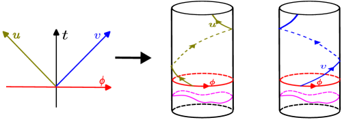
Figure 2: The mapping from the plane to the cylinder. In the first cylinder, the time direction is along the image of the u- axis. On this cylinder, the left-handed modes live, while the second cylinder contains the right-handed modes.

where, for simplicity, we assume that in the first equality, the integrand inside the absolute value does not change sign, and therefore, we can pull the absolute value out of the integral. So far, we assume that the $u$ and $v$ directions are defined over the plane. Moreover, $g^{(0)}_{uu}$ and $g^{(0)}_{vv}$ remain constant as we move along $v$ and $u$ directions, respectively. Taking $(u,v)=(t-\phi,t+\phi)$, compactifying the $\phi$ direction transforms the plane to the cylinder. Note that the two integrals in 4.92 are separate, and $u$ and $v$ are causal directions. To keep them causal, we will consider two cylinders where non-compact directions are associated with $u$ and $v$; see figure 2. Moreover, on each cylinder, we can take the integral over the compact direction; we can write $(u,v)=(u,u+2\phi)$ and take the integral over $\phi\in(0,2\pi)$ while $u$ is fixed, which leads to

$$\frac{1}{16\pi G}\int_{0}^{2\pi}~{}d\phi~{}\int~{}du~{}g^{(0)}_{uu}(u)=\frac{1}{8G}\int~{}du~{}g^{(0)}_{uu}(u),$$ (4.93)

while, for $g^{(0)}_{vv}(v)$ we have:

$$-\frac{1}{32\pi G}\int dudv~{}g^{(0)}_{vv}(v)=\frac{1}{32\pi G}\int_{0}^{2\pi}~{}d\phi~{}\int~{}dv~{}g^{(0)}_{vv}(v)=\frac{1}{8G}\int~{}dv~{}g^{(0)}_{vv}(v).$$ (4.94)

Note that in taking the integral over $u$ direction while $v$ is constant, there is a relative minus sign as the $\phi$ direction is reversed. Therefore, the result will take the following form:

$$S_{GHY}=\frac{1}{8G}\int~{}du~{}g^{(0)}_{uu}(u)+\frac{1}{8G}\int~{}dv~{}g^{(0)}_{vv}(v),$$ (4.95)

Now, if we take $(g^{(0)}_{uu},g^{(0)}_{vv})=(-\operatorname{Sch}(e^{\phi_{+}(u)}),-\operatorname{Sch}(e^{\phi_{-}(v)}))$, after the Wick rotation the GHY action will take the following form,

$$I_{E}=-\frac{1}{8G}\int_{0}^{\beta_{+}}~{}du_{E}~{}\operatorname{Sch}(e^{i\phi_{+}})-\frac{1}{8G}\int_{0}^{\beta_{-}}~{}dv_{E}~{}\operatorname{Sch}(e^{i\phi_{-}}).$$ (4.96)

The above action is defined over the disjoint union of two circles of circumference $\beta_{\pm}$.

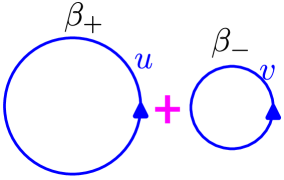
Figure 3:

computing the action over the solution $\phi_{\pm}=\frac{2\pi}{\beta_{\pm}}$ leads to:

$$I_{E}=I_{+}+I_{-},~{}~{}~{}~{}~{}~{}I_{\pm}=-\frac{\pi^{2}}{4G}\frac{1}{\beta_{\pm}}$$ (4.97)

The above is precisely equal to 3.73, computed in the first scheme in which both bulk and boundary will contribute. This will imply the degrees of freedom associated with the black hole geometry are located on the boundary. For our later convenience, we rewrite the thermodynamic quantities as follows:

$$M=H^{\operatorname{ADM}}_{+}+H^{\operatorname{ADM}}_{-},~{}~{}~{}~{}J=H^{\operatorname{ADM}}_{-}-H^{\operatorname{ADM}}_{+},~{}~{}~{}~{}~{}~{}H^{\operatorname{ADM}}_{\pm}=\frac{\pi^{2}}{4G}\,\frac{1}{\beta_{\pm}^{2}},$$ (4.98)

$$S=S_{+}+S_{-},~{}~{}~{}~{}~{}S_{\pm}=\frac{\pi^{2}}{2G}\frac{1}{\beta_{\pm}}.$$

Also, the on-shell action takes the following form,

$$S_{\operatorname{on-shell}}=S_{\operatorname{on-shell}+}+S_{\operatorname{on-shell}-},~{}~{}~{}~{}~{}S_{\operatorname{on-shell}\pm}=\beta_{\pm}H_{\pm}-S_{\pm}=-\frac{\pi^{2}}{4G}\frac{1}{\beta_{\pm}}.$$ (4.99)

Notice that the induced metric on the physical boundary associated with the non-rotating BTZ without any fluctuations becomes a degenerate induced metric, i.e., 4.91 in this scheme, and so the GHY action 4.92 is not well defined. This is related to the fact that in this case, the two Euclidean circles in figure 3 associated with left-moving and right-moving modes become indistinguishable. This can be avoided if we consider the non-rotating BTZ as the $J\rightarrow 0$ limit of the Kerr-BTZ thermofield-double. Consider the thermofield-double

$$\Big{|}\operatorname{TFD}\Big{\rangle}=\frac{e^{-\frac{\beta_{+}H_{+}+\beta_{-}H_{-}}{2}}}{\mathcal{Z}^{\frac{1}{2}}}~{}\sum_{n}~{}\ket{E_{n},J_{n}}_{R}\otimes\ket{E_{n}^{*},J_{n}^{*}}_{L},~{}~{}~{}~{}~{}~{}H_{\pm}=\frac{H\mp J}{2},$$ (4.100)

which is associated with the BTZ black hole in the bulk[19]. The state is written in terms of the eigenstates of the Hamiltonian and the angular momentum. The associated partition function is:

$$\mathcal{Z}=\Tr\Big(e^{-(\beta_{-}H_{-}+\beta_{+}H_{+})}\Big{missing}).$$ (4.101)

The relation between Bosonic fields acting on the left and right side of the thermofield-double is:

$$O_{L}(iu,iv)\Big{|}TFD\Big{\rangle}=O_{R}(iu-\frac{\beta_{+}}{2},iv-\frac{\beta_{-}}{2})\Big{|}TFD\Big{\rangle}.$$ (4.102)

The above relation is written in the Euclidean signature where $(u,v)=(t-\phi,\,t+\phi)$. Moreover, the Euclidean two-point function of the fields at finite temperature is given by [19, 48]:

$$\Big{\langle}\operatorname{TFD}\Big{|}O_{R}(iu_{1},iv_{1})O_{R}(iu_{2},iv_{2})\Big{|}\operatorname{TFD}\Big{\rangle}=G_{\beta_{\pm}}(iu_{1},iv_{1},iu_{2},iv_{2})$$ (4.103)

$$~{}~{}~{}~{}~{}~{}~{}~{}~{}~{}~{}~{}~{}~{}~{}~{}~{}~{}~{}~{}~{}~{}~{}~{}~{}~{}~{}~{}~{}~{}~{}~{}~{}~{}~{}~{}~{}~{}~{}~{}~{}=\sum_{n=-\infty}^{\infty}~{}\frac{b}{\Big{(}\frac{\beta_{+}J_{+}}{\pi}\sin\frac{i\pi(u_{1}-u_{2}+2n\pi)}{\beta_{+}}\Big{)}^{2\Delta_{+}}\Big{(}\frac{\beta_{-}J_{-}}{\pi}\sin\frac{i\pi(v_{1}-v_{2}-2n\pi)}{\beta_{-}}\Big{)}^{2\Delta_{-}}}.$$

Here, $J_{\pm}$ are parameters with dimension of energy to make the denominator dimensionless. Also, the sum over $n$ confirms the invariance of the two-point function under $\phi\rightarrow\phi+2\pi$.

The properties of the Schwarzian action and its contribution to the four-point function of fields have been studied in detail in [14, 15]. However, before giving our ansatz for the coupling of the Schwarzian modes to the two- point function, we first define $\theta^{+}=\frac{2\pi u_{E}}{\beta_{+}}$ , $\theta^{-}=\frac{2\pi v_{E}}{\beta_{-}}$, where $(u_{E},v_{E})=(iu,iv)$, and $\theta^{\pm(n)}=\theta^{\pm}\mp\frac{4\pi^{2}i\,n}{\beta_{\pm}}$. The two-point function will take the following form:

$$G_{\beta_{\pm}}\Big{(}\theta^{+}_{1},\theta^{-}_{1},\theta^{+}_{2},\theta^{-}_{2}\Big{)}=\frac{b}{J_{+}^{2\Delta_{+}}J_{-}^{2\Delta_{-}}}\lim_{N\rightarrow\infty}\frac{1}{(2N+1)}\sum_{m={-N}}^{N}\sum_{n=-\infty}^{\infty}~{}G_{nm}\Big{(}\theta_{1}^{+},\theta_{2}^{+}\Big{)}G_{nm}\Big{(}\theta_{1}^{-},\theta_{2}^{-}\Big{)},$$ (4.104)

$$G_{nm}\Big{(}\theta_{1}^{+},\theta_{2}^{+}\Big{)}=\frac{1}{~{}~{}\Big{(}2\sin\frac{\theta^{+(n)}_{1}-\theta^{+(m)}_{2}}{2}\Big{)}^{2\Delta_{+}}},~{}~{}~{}~{}~{}~{}G_{nm}\Big{(}\theta_{1}^{-},\theta_{2}^{-}\Big{)}=\frac{1}{~{}~{}\Big{(}2\sin\frac{\theta^{-(n)}_{1}-\theta^{-(m)}_{2}}{2}\Big{)}^{2\Delta_{-}}},$$

where we just summed up $2N+1$ copies of the original two-point function. This way, the two-point function will take a symmetric form. Clearly, the terms $G_{nm}$ are only functions of $n-m$. Now, the reparametrization modes will couple to the two-point function as follows:

$$G_{\beta_{\pm}}\Big{(}\varphi_{1}^{+},\varphi_{1}^{-},\varphi^{+}_{2},\varphi^{-}_{2}\Big{)}=\frac{b}{J_{+}^{2\Delta_{+}}J_{-}^{2\Delta_{-}}}\lim_{N\rightarrow\infty}\frac{1}{(2N+1)}\sum_{m={-N}}^{N}\sum_{n=-\infty}^{\infty}G_{nm}\Big{(}\varphi(\theta_{1}^{+}),\varphi(\theta_{2}^{+})\Big{)}G_{nm}\Big{(}\varphi^{-}(\theta_{1}^{-}),\varphi^{-}(\theta_{2}^{-})\Big{)}$$ (4.105)

$$G_{nm}\Big{(}\varphi^{\pm}(\theta_{1}^{\pm}),\varphi^{\pm}(\theta_{2}^{\pm})\Big{)}=\frac{\Big{(}\varphi^{\prime}(\theta_{1}^{\pm(n)})\Big{)}^{\Delta_{\pm}}\Big{(}\varphi^{\prime}(\theta_{2}^{\pm(m)})\Big{)}^{\Delta_{\pm}}}{~{}~{}\Big{(}2\sin\frac{\varphi(\theta_{1}^{\pm(n)})-\varphi(\theta^{\pm(m)}_{2})}{2}\Big{)}^{2\Delta_{\pm}}}.$$

Note that this way of dressing the two-point function by the reparametrization modes saves the periodicity of angular direction $\phi$ after the Wick rotation.

4.2 Contribution of Schwarzian modes to the four-point function

In this section, we will closely follow [14, 18]. Expanding the Schwarzian action around the saddle point, $\varphi^{\pm}(\theta^{\pm})=\theta^{\pm}+\delta\varphi^{\pm}(\theta^{\pm})$ to second order has the following form

$$I_{\pm}=-\frac{\pi}{4G\beta_{\pm}}\int_{0}^{2\pi}d\theta^{\pm}~{}\Big{(}\frac{1}{2}-\frac{1}{2}\Big{(}(\delta{\varphi^{\pm}}^{\prime\prime})^{2}-(\delta{\varphi^{\pm}}^{\prime})^{2}\Big{)}\Big{)},$$ (4.106)

where the fluctuations have the following Fourier series

$$\delta\varphi^{\pm}(\theta^{\pm})=\sum_{n}~{}\delta\varphi^{\pm}_{n}~{}e^{in\theta^{\pm}}.$$ (4.107)

Plugging back, the two-point function of the Fourier modes takes the following form:

$$\Big{\langle}\delta\varphi_{n}^{\pm}\,\,\delta\varphi^{\pm}_{m}\Big{\rangle}=\frac{1}{S_{\pm}}\frac{\delta_{m+n}}{n^{2}(n^{2}-1)},~{}~{}~{}~{}n\neq 0,\pm 1.$$ (4.108)

On the other hand, we have:

$$\delta G_{\beta_{\pm}}\Big{(}\theta_{1}^{+},\theta_{1}^{-},\theta^{+}_{2},\theta^{-}_{2}\Big{)}=$$ (4.109)

$$\frac{b}{J_{+}^{2\Delta_{+}}J_{-}^{2\Delta_{-}}}\lim_{N\rightarrow\infty}\frac{1}{(2N+1)}\sum_{m={-N}}^{N}\sum_{n=-\infty}^{\infty}G_{nm}\Big{(}\theta_{1}^{+},\theta_{2}^{+}\Big{)}G_{nm}\Big{(}\theta_{1}^{-},\theta_{2}^{-}\Big{)}\bigg{(}\frac{\delta G_{nm}(\theta_{1}^{+},\theta_{2}^{+})}{G_{nm}(\theta_{1}^{+},\theta_{2}^{+})}+\frac{\delta G_{nm}(\theta_{1}^{-},\theta_{2}^{-})}{G_{nm}(\theta_{1}^{-},\theta_{2}^{-})}\bigg{)},$$

$$\frac{\delta G_{nm}(\theta_{1}^{\pm},\theta_{2}^{\pm})}{G_{nm}(\theta_{1}^{\pm},\theta_{2}^{\pm})}=\Delta^{\pm}\Big{(}\delta\varphi^{\pm}(\theta_{1}^{\pm(n)})+\delta\varphi^{\pm}(\theta_{2}^{\pm(m)})-\frac{\delta\varphi^{\pm}(\theta_{1}^{\pm(n)})-\delta\varphi^{\pm}(\theta^{\pm(m)})}{\tan\frac{\theta_{1}^{\pm(n)}-\theta_{2}^{\pm(m)}}{2}}\Big{)}.$$

The value of the time-ordered four-point function will take the form:

$$\bigg{\langle}\frac{\delta G_{nm}(\theta_{1}^{\pm},\theta_{2}^{\pm})}{G_{nm}(\theta_{1}^{\pm},\theta_{2}^{\pm})}\frac{\delta G_{pq}(\theta_{3}^{\pm},\theta_{4}^{\pm})}{G_{pq}(\theta_{3}^{\pm},\theta_{4}^{\pm})}\bigg{\rangle}=\frac{4\,\Delta_{\pm 1}\Delta_{\pm 2}}{S_{\pm}}\bigg{(}1-\frac{\frac{\theta_{1}^{\pm(n)}-\theta_{2}^{\pm(m)}}{2}}{\tan\frac{\theta_{1}^{\pm(n)}-\theta_{2}^{\pm(m)}}{2}}\bigg{)}\bigg{(}1-\frac{\frac{\theta_{3}^{\pm(p)}-\theta_{4}^{\pm(q)}}{2}}{\tan\frac{\theta_{3}^{\pm(p)}-\theta_{4}^{\pm(q)}}{2}}\bigg{)},$$ (4.110)

$$~{}~{}~{}~{}~{}~{}~{}~{}~{}~{}~{}~{}~{}~{}~{}~{}~{}~{}~{}~{}~{}~{}~{}~{}~{}~{}~{}~{}~{}~{}~{}~{}~{}~{}~{}~{}~{}~{}~{}~{}~{}~{}~{}~{}~{}~{}~{}~{}~{}~{}~{}~{}~{}~{}~{}~{}~{}~{}~{}~{}~{}~{}~{}~{}~{}~{}~{}~{}~{}~{}~{}~{}~{}~{}~{}~{}~{}~{}~{}~{}~{}~{}~{}~{}~{}~{}~{}~{}~{}~{}~{}~{}~{}~{}~{}~{}~{}~{}~{}~{}~{}~{}~{}~{}\theta_{1}>\theta_{2}>\theta_{3}>\theta_{4}.$$

Note that the above expectation value, similar to the two-point function, is only the function of time differences $\theta^{\pm}_{1}-\theta^{\pm}_{2}$ and $\theta^{\pm}_{3}-\theta^{\pm}_{4}$. In particular, it is a function of both $n-m$ and $p-q$. Therefore, to compute the four point function we can simply write,

$$\bigg{\langle}O^{i}(\theta_{1})O^{i}(\theta_{2})O^{j}(\theta_{3})O^{j}(\theta_{4})\bigg{\rangle}=\sum_{n,m}~{}\frac{4\Delta_{-1}\Delta_{-2}}{S_{-}}~{}G_{n}(\theta^{-}_{1},\theta^{-}_{2})G_{m}(\theta^{-}_{3},\theta^{-}_{4})\mathcal{F}_{n}(\theta^{-}_{1}-\theta^{-}_{2})\mathcal{F}_{m}(\theta^{-}_{3}-\theta^{-}_{4})$$ (4.111)

$$~{}~{}~{}~{}~{}~{}~{}~{}~{}~{}~{}~{}~{}~{}~{}~{}~{}~{}~{}~{}~{}~{}~{}~{}~{}~{}~{}~{}~{}~{}~{}~{}~{}~{}~{}~{}~{}~{}+\sum_{n,m}~{}\frac{4\Delta_{+1}\Delta_{+2}}{S_{+}}~{}G_{n}(\theta^{+}_{1},\theta^{+}_{2})G_{m}(\theta^{+}_{3},\theta^{+}_{4})\mathcal{F}_{n}(\theta^{+}_{1}-\theta^{+}_{2})\mathcal{F}_{m}(\theta^{+}_{3}-\theta^{+}_{4}),$$

$$G_{n}(\theta^{\pm}_{1},\theta^{\pm}_{2})=\frac{1}{~{}~{}\Big{(}2\sin\frac{\theta^{\pm(n)}_{1}-\theta^{\pm}_{2}}{2}\Big{)}^{2\Delta_{\pm}}},~{}~{}~{}~{}~{}~{}~{}\mathcal{F}_{n}(\theta^{\pm}_{1}-\theta^{\pm}_{2})=\bigg{(}1-\frac{\frac{\theta_{1}^{\pm(n)}-\theta_{2}^{\pm}}{2}}{\tan\frac{\theta_{1}^{\pm(n)}-\theta_{2}^{\pm}}{2}}.\bigg{)}$$

For the computation of the out-of-time-ordered four-point correlation function, the Gaussian approximation is not suitable; It will take the following form:

$$\bigg{\langle}\frac{\delta G_{nm}(\theta_{1}^{\pm},\theta_{2}^{\pm})}{G_{nm}(\theta_{1}^{\pm},\theta_{2}^{\pm})}\frac{\delta G_{pq}(\theta_{3}^{\pm},\theta_{4}^{\pm})}{G_{pq}(\theta_{3}^{\pm},\theta_{4}^{\pm})}\bigg{\rangle}\sim\frac{\sin(\frac{\theta^{\pm(n)}_{1}+\theta^{\pm(m)}_{2}}{2}-\frac{\theta^{\pm(p)}_{3}+\theta^{\pm(q)}_{4}}{2})}{\sin(\frac{\theta^{\pm(n)}_{1}-\theta^{\pm(m)}_{2}}{2})\sin(\frac{\theta^{\pm(p)}_{3}-\theta^{\pm(q)}_{4}}{2})}.$$ (4.112)

Going to the Lorentzian signature and taking $\theta^{\pm(n)}=\frac{2\pi i}{\beta_{\pm}}(t\mp(\phi+2\pi n))$, for fixed $(p,q)$, if we shift both indices $n,m$ by an integer, the denominator does not change while the numerator will increase exponentially. However, it is possible to compute the exact solution. The answer is [18, 49]:

$$\bigg{\langle}O(t_{1},\phi_{1})O(t_{3},\phi_{3})O(t_{2},\phi_{2})O(t_{4},\phi_{4})\bigg{\rangle}=\lim_{M,N\rightarrow\infty}\frac{1}{(2N+1)(2M+1)}\sum_{m\in-N}^{N}\sum_{q\in-M}^{M}\sum_{n,p\in-\infty}^{\infty}$$ (4.113)

$$G_{n,m}(u_{1},u_{2})G_{n,m}(v_{1},v_{2})G_{p,q}(u_{3},u_{4})G_{p,q}(v_{3},v_{4})\times$$

$$\Big{(}iC^{+}_{m,n,p,q}\Big{)}^{-2\Delta_{1}^{+}}U(2\Delta^{+}_{1},1-2\Delta_{2}^{+}+2\Delta_{1}^{+},\frac{1}{iC_{m,n,p,q}})\times\Big{(}iC^{-}_{m,n,p,q}\Big{)}^{-2\Delta_{1}^{-}}U(2\Delta^{-}_{1},1-2\Delta_{2}^{-}+2\Delta_{1}^{-},\frac{1}{iC_{m,n,p,q}}),$$

$$C^{+}_{n,m,p,q}=\frac{\pi}{S_{+}}\frac{e^{\frac{\pi}{\beta_{+}}(u_{1}^{(n)}+u_{2}^{(m)}-u_{3}^{(p)}-u^{(q)}_{4})}}{\Big{(}2\sinh\frac{\pi}{\beta_{+}}(u_{1}^{(n)}-u^{(m)}_{2})\Big{)}\Big{(}2\sinh\frac{\pi}{\beta_{+}}(u_{3}^{(p)}-u^{(q)}_{4})\Big{)}},$$

$$C^{-}_{n,m,p,q}=\frac{\pi}{S_{-}}\frac{e^{\frac{\pi}{\beta_{-}}(v_{1}^{(n)}+v_{2}^{(m)}-v_{3}^{(p)}-v^{(q)}_{4})}}{\Big{(}2\sinh\frac{\pi}{\beta_{-}}(v_{1}^{(n)}-v^{(m)}_{2})\Big{)}\Big{(}2\sinh\frac{\pi}{\beta_{-}}(v_{3}^{(p)}-v^{(q)}_{4})\Big{)}}.$$

Here, $U(a,b,x)$ is a confluent hypergeometric function of the second kind, and the terms with superscripts plus and minus are associated with left-handed and right-handed modes.

4.3 Evolution of the thermofield-double state by coupling its both sides

Now, consider the following interaction Hamiltonian that couples both sides of the thermofield-double:

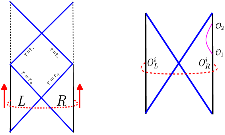
Figure 4:

$$H_{int}=\frac{g}{N}\int_{0}^{2\pi}~{}d\phi~{}O^{i}_{L}(\phi)O^{i}_{R}(\phi),~{}~{}~{}~{}~{}~{}i=1,\cdots,N$$ (4.114)

Here the field $O^{i}$ is Bosonic with dimension $(\Delta_{+},\Delta_{-})$. There is an implicit sum over the index $i$ that we dropped for convenience. We are interested in the setup where the right field evolves forward in time while the left field evolves backward. The corresponding evolution operator is

$$U_{I}(t)=\mathfrak{T}~{}\exp\Big(-\frac{ig}{N}\int_{0}^{2\pi}d\phi\int_{0}^{t}~{}du~{}O^{i}_{R}(u,\phi)O^{i}_{L}(-u,\phi)\Big{missing}).$$ (4.115)

Here, $\mathfrak{T}$ is the time ordering operator. To compute the entanglement entropy, one can use the replica method to compute the von Neumann entropy

$$S_{EE}=-\partial_{s}~{}\ln\Tr\rho^{s}(t)\Big{|}_{s=1}.$$ (4.116)

The computation is exactly the same as in [23], and we will not repeat it here. The final answer is:

$$\frac{\Delta S_{EE}}{S}=-\frac{4\pi g}{S}~{}\int_{0}^{t}~{}du~{}\frac{d}{ds}\imaginary G_{s\beta_{\pm}}\Big{(}2iu+\frac{\beta_{+}}{2},2iu+\frac{\beta_{-}}{2}\Big{)}\bigg{|}_{s=1}$$ (4.117)

$$=-\frac{\pi gb}{S}~{}\Big{(}\frac{\pi}{\beta_{-}J_{-}}\Big{)}^{2\Delta_{-}}\Big{(}\frac{\pi}{\beta_{+}J_{+}}\Big{)}^{2\Delta_{+}}\sum_{n}\int_{0}^{t}du~{}\bigg{[}\beta_{+}\bigg{(}\frac{1}{\cosh^{2\Delta_{+}}\frac{2\pi u+2n\pi^{2}}{\beta_{+}}}\bigg{)}^{\prime}\frac{1}{\cosh^{2\Delta_{-}}\frac{2\pi u-2n\pi^{2}}{\beta_{-}}}$$

$$~{}~{}~{}~{}~{}~{}~{}~{}~{}~{}~{}~{}~{}~{}~{}~{}~{}~{}~{}~{}~{}~{}~{}~{}~{}~{}~{}~{}~{}~{}~{}~{}~{}~{}~{}~{}~{}~{}~{}~{}~{}~{}~{}~{}~{}~{}~{}~{}~{}~{}~{}~{}~{}~{}~{}~{}+\beta_{-}\bigg{(}\frac{1}{\cosh^{2\Delta_{-}}\frac{2\pi u-2n\pi^{2}}{\beta_{-}}}\bigg{)}^{\prime}\frac{1}{\cosh^{2\Delta_{+}}\frac{2\pi u+2n\pi^{2}}{\beta_{+}}}\bigg{]},$$

where, in the last line, the derivative is with respect to $u$. In the special case where the angular momentum $J$ vanishes, the integrand becomes a total derivative, and the integral can be evaluated $(\beta_{+}=\beta_{-}=\beta)$

$$\Delta S_{EE}=\frac{\pi^{2}bg}{(J_{+}J_{-})^{1/2}}\Big{(}\frac{\pi}{\beta(J_{+}J_{-})^{1/2}}\Big{)}^{2\Delta-1}$$ (4.118)

$$~{}~{}~{}~{}~{}~{}~{}~{}~{}~{}~{}~{}~{}~{}~{}~{}~{}~{}~{}~{}~{}~{}~{}~{}~{}~{}~{}~{}~{}~{}~{}~{}~{}~{}~{}~{}~{}~{}~{}\times\sum_{n}\bigg{(}\frac{1}{\cosh^{2(\Delta_{+}+\Delta_{-})}\frac{2\pi^{2}n}{\beta}}-\frac{1}{\cosh^{2\Delta_{-}}(\frac{2\pi u}{\beta}+\frac{2\pi^{2}n}{\beta})\cosh^{2\Delta_{+}}(\frac{2\pi u}{\beta}-\frac{2\pi^{2}n}{\beta})}\bigg{)}$$

However, from $\Delta S_{EE}$ we are not allowed to read the change in the temperature, as it must be read from the change in the coarse-grained entropy. It is easier to derive it by evaluating the two-point function after the system reaches equilibrium. Therefore, we need to compute the modified two-point function of two probing fields that live on the right side; see figure 4. Using 4.115, it takes the following form:

$$\Big{\langle}\widetilde{TFD}\Big{|}\,\mathcal{O}(t_{1},\phi_{1})\mathcal{O}(t_{2},\phi_{2})\Big{|}\widetilde{TFD}\Big{\rangle}=\Big{\langle}TFD\Big{|}U_{I}(t_{0},t_{2})\,\mathcal{O}(t_{1},\phi_{1})U_{I}(t_{2},t_{1})\mathcal{O}(t_{2},\phi_{2})U_{I}(t_{1},t_{0})\Big{|}TFD\Big{\rangle}$$ (4.119)

To leading order, the evolution operator is

$$U_{I}(t,t_{0})=1-\frac{ig}{N}\sum_{i}\int_{0}^{2\pi}~{}d\phi~{}\int_{t_{0}}^{t}~{}du~{}O^{i}_{R}(u,\phi)O^{i}_{L}(-u,\phi)$$ (4.120)

By plugging back into the two-point function 4.119, it can be written in terms of the four-point functions,

$$\widetilde{G}(t_{2},\phi_{2};t_{1},\phi_{1})=\Big{\langle}\widetilde{TFD}\Big{|}\,\mathcal{O}(t_{2},\phi_{2})\mathcal{O}(t_{1},\phi_{1})\Big{|}\widetilde{TFD}\Big{\rangle}=\Big{\langle}\,\mathcal{O}(it_{2},\phi_{2})\mathcal{O}(it_{1},\phi_{1})\Big{\rangle}$$ (4.121)

$$-\frac{ig}{N}\sum_{i}\int_{0}^{2\pi}~{}d\phi~{}\Bigg{[}\int_{t_{0}}^{t_{1}}~{}du~{}\Big{\langle}\mathcal{O}(it_{2},\phi_{2})\mathcal{O}(it_{1},\phi_{1})O^{i}_{R}(iu,\phi)O^{i}_{L}(-iu,\phi)\Big{\rangle}$$

$$~{}~{}~{}~{}~{}~{}~{}~{}~{}~{}~{}~{}~{}~{}~{}~{}~{}~{}-\int_{t_{0}}^{t_{2}}du\Big{\langle}O^{i}_{R}(iu,\phi)O^{i}_{L}(-iu,\phi)\mathcal{O}(it_{2},\phi_{2})\mathcal{O}(it_{1},\phi_{1})\Big{\rangle}$$

$$~{}~{}~{}~{}~{}~{}~{}~{}~{}~{}~{}~{}~{}~{}~{}~{}~{}~{}+\int_{t_{1}}^{t_{2}}du\Big{\langle}\mathcal{O}(it_{2},\phi_{2})O^{i}_{R}(iu,\phi)O^{i}_{L}(-iu,\phi)\mathcal{O}(it_{1},\phi_{1})\Big{\rangle}\Bigg{]}$$

The computation is straightforward and will be postponed to Appendix B. For $u_{1(2)}=t_{1(2)}-\phi_{1(2)}$ the final answer for $\beta_{\pm}\ll t_{i}\ll\beta_{\pm}\ln S$ is

$$\widetilde{G}(t_{1},\phi_{1};t_{2},\phi_{2})=\sum_{m}G_{m}(iu_{12},iv_{12})\Bigg{[}1-\frac{2\Delta_{+}\delta\beta_{+}}{\beta_{+}}\mathcal{F}_{m}(\frac{2\pi iu_{12}}{\beta_{+}})-\frac{2\Delta_{-}\delta\beta_{-}}{\beta_{-}}\bar{\mathcal{F}}_{m}(\frac{2\pi iv_{12}}{\beta_{-}})\Bigg{]}$$ (4.122)

If we define: $(t_{1}<t_{2})$

$$A_{+}(t_{1})=-g\,b\,\pi\Big{(}\frac{\pi}{\beta_{-}J_{-}}\Big{)}^{2\Delta_{-}}\Big{(}\frac{\pi}{\beta_{+}J_{+}}\Big{)}^{2\Delta_{+}}\sum_{n}\int_{0}^{t_{1}}du~{}\Big{(}\frac{1}{\cosh^{2\Delta_{+}}\frac{2\pi u^{(n)}}{\beta_{+}}}\Big{)}^{\prime}\frac{1}{\cosh^{2\Delta_{-}}\frac{2\pi u^{(-n)}}{\beta_{-}}},$$ (4.123)

$$A_{-}(t_{1})=-g\,b\,\pi\Big{(}\frac{\pi}{\beta_{-}J_{-}}\Big{)}^{2\Delta_{-}}\Big{(}\frac{\pi}{\beta_{+}J_{+}}\Big{)}^{2\Delta_{+}}\sum_{n}\int_{0}^{t_{1}}du~{}\Big{(}\frac{1}{\cosh^{2\Delta_{-}}\frac{2\pi u^{(-n)}}{\beta_{-}}}\Big{)}^{\prime}\frac{1}{\cosh^{2\Delta_{+}}\frac{2\pi u^{(n)}}{\beta_{+}}}.$$

From the above expressions, we can read the temperature change:

$$\frac{\delta\beta_{+}}{\beta_{+}}=-\frac{\beta_{+}}{S_{+}}~{}A_{+}(t_{1}\rightarrow\infty),$$ (4.124)

$$\frac{\delta\beta_{-}}{\beta_{-}}=-\frac{\beta_{-}}{S_{-}}A_{-}(t_{1}\rightarrow\infty).$$

From this, we conclude that:

$$A_{\pm}(t_{1})=-\frac{\pi^{2}}{2G}\frac{\delta\beta_{\pm}}{\beta^{3}_{\pm}}=\frac{\pi^{2}}{4G}~{}\delta~{}\Big{(}\frac{1}{\beta^{2}_{\pm}}\Big{)}=\Delta H^{\operatorname{ADM}}_{\pm}.$$ (4.125)

On the other hand, variation of the relation yields:

$$\Delta S_{\pm}=-\frac{\pi^{2}}{2G}\Big{(}\frac{\delta\beta_{\pm}}{\beta^{2}_{\pm}}\Big{)}=\frac{\pi^{2}}{2G}\frac{A_{\pm}(t_{1})}{S_{\pm}}=\beta_{\pm}A_{\pm}(t_{1}),$$ (4.126)

which is the amount that the coarse-grained entropy changes, whereas the amount of entanglement entropy change 4.117 equals:

$$\Delta S_{EE}=\beta_{+}A_{+}(t_{1})+\beta_{-}A_{-}(t_{1}).$$ (4.127)

To understand the physical meaning of 4.127 and 4.124 one should notice that $A_{\pm}(t)\propto\Delta\Big{\langle}H_{\pm}\Big{\rangle}$. More accurately:

$$\Big{\langle}\widetilde{TFD}(t)\Big{|}~{}H_{\pm}~{}\Big{|}\widetilde{TFD}(t)\Big{\rangle}-\Big{\langle}H_{\pm}\Big{\rangle}=-2\pi ig\int_{0}^{t}\Big{\langle}TFD\Big{|}\Big{[}H_{\pm},O_{R}(u)\Big{]}O_{L}(u)\Big{|}TFD\Big{\rangle}$$ (4.128)

$$=-2\pi g\int_{0}^{t}~{}du~{}\Big{\langle}TFD\Big{|}\partial_{u_{\pm}}O_{R}(iu,\phi)O_{L}(-iu,\phi)\Big{|}TFD\Big{\rangle}=A_{\pm}(t).$$

Hence, after the system reaches equilibrium, not only are the coarse-grained entropy and entanglement entropy equal, we, in fact, can associate a well-defined ADM mass and angular momentum

$$M^{\operatorname{ADM}}=\Big{\langle}\widetilde{\operatorname{TFD}}\Big{|}\,H\,\Big{|}\widetilde{\operatorname{TFD}}\Big{\rangle},~{}~{}~{}~{}~{}~{}J^{\operatorname{ADM}}=\Big{\langle}\widetilde{\operatorname{TFD}}\Big{|}\,J\,\Big{|}\widetilde{\operatorname{TFD}}\Big{\rangle}$$ (4.129)

to the resulting state. This confirms that the effective degrees of freedom associated with the black hole in the bulk are the reparametrization modes that live on the boundary of AdS3.

4.4 Considering the general boundary condition

Now, as our second example, we consider the general boundary condition 3.51, and we are looking for a solution for $h_{uv}^{(1)}$ that extremizes the GHY action on the physical boundary $r=\varepsilon$. As we studied the asymptotic form of the trace of the second fundamental form, the extremization procedure, in fact, corresponds to extremizing the volume term in the action in the limit $\varepsilon\rightarrow 0$,

$$\frac{\delta h}{\delta h^{(1)}_{uv}(\varepsilon)}=0$$ (4.130)

Considering the following expansion

$$h^{(1)}_{uv}(\varepsilon)=\frac{h^{(11)}_{uv}(u,v)}{\varepsilon}+h^{(10)}_{uv}(u,v)$$ (4.131)

Then to leading order, we have:

$$h=\frac{e^{-2\varphi}\Big{(}h_{uv}^{(11)}-2e^{\varphi}\Big{)}^{4}}{64\varepsilon^{4}}+O(\frac{1}{\varepsilon^{3}})\rightarrow\boxed{h_{uv}^{(11)}=2e^{\varphi}},~{}~{}~{}~{}~{}~{}\varphi=\varphi_{1}+\varphi_{2}.$$ (4.132)

Plugging back this value into the metric will cancel all the divergences of the metric on the physical boundary,

$$g_{uu}=\Big{(}\frac{1}{r}-\frac{1}{\varepsilon}\Big{)}h^{(1)}_{uu}+h^{(0)}_{uu},$$ (4.133)

$$g_{vv}=\Big{(}\frac{1}{r}-\frac{1}{\varepsilon}\Big{)}h^{(1)}_{vv}+h^{(0)}_{vv}$$

$$g_{uv}=-e^{\varphi}\Big{(}\frac{1}{r}-\frac{1}{\varepsilon}\Big{)}^{2}+\Big{(}\frac{1}{r}-\frac{1}{\varepsilon}\Big{)}h^{(10)}_{uv}+h^{(0)}_{uv}$$

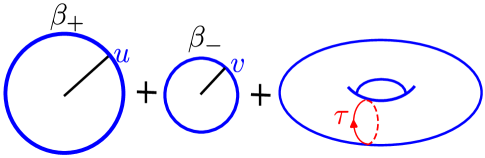
Figure 5:

Notice that the above form of the metric is valid only close to $r=\varepsilon$. In this case, we expect the Euclidean manifold to be promoted to two circles where the reparametrization modes live plus a torus where possibly, other non-chiral metric components live. Equation 4.130 becomes simple in special case where $\varphi_{1}=\varphi_{2}$,

$$h^{(10)}_{uv}=e^{\varphi_{1}}\Big{(}\partial_{v}\varphi_{1}+\partial_{u}\varphi_{1}\Big{)}$$ (4.134)

Plugging back into the metric will cancel the $\varphi_{1}$ terms in the metric components, and hence, we will end up with the above metric components with

$$h_{uu}^{(0)}=\frac{1}{2}g^{(0)}_{uu},~{}~{}~{}~{}~{}h^{(0)}_{vv}=\frac{1}{2}g^{(0)}_{vv},~{}~{}~{}~{}~{}h^{(0)}_{uv}=\frac{1}{4}\Big{(}g^{(0)}_{uu}+g^{(0)}_{vv}\Big{)},$$ (4.135)

which is the same induced metric on the physical boundary as the one with $\varphi_{1}=\varphi_{2}=0$. Therefore, in the case where $\varphi_{1}=\varphi_{2}$, using the second scheme will erase the effect of the Liouville field on the physical boundary.

5 Discussion

The integral of the trace of the second fundamental form over the boundary that surrounds the bulk was proposed by York, Hawking, and Gibbons to have a consistent variation of the Einstein-Hilbert action with the Dirichlet boundary condition. On the other hand, from the holography point of view, one expects the true degrees of freedom, such as the degrees of freedom associated with thermofield-double, to live on the physical boundary of AdS. The GHY action is the right candidate to describe the dynamics of such effective degrees of freedom. However, there are two obstacles. First and foremost, the action is divergent. Second, the regularized action depends on the choice of coordinate. In this paper, we had a proposal for overcoming both problems. We first employed a coordinate system that has two time coordinates 1.41.5 (more precisely, two causal coordinates). One time is associated with boundary evolution, often called boundary time. In the direction of the second time, boundary degrees of freedom evolve deep into the bulk. In this coordinate system, we can solve Einstein’s equation 3.51 with the given boundary condition 1.4. To regularize the action, we considered two particular schemes. In the first scheme, we added the Einstein-Hilbert counter term to the GHY action. The value of the action is proportional to the volume of the bulk. The most important con of this regularization is that it is non-local; e.g., it considers the effect of a possible horizon in the bulk. Another disadvantage is that “attaching the bulk to the boundary” by taking the integral over its volume fixes the boundary topology( in our case, the first scheme fixes the boundary to have genus one). Then a possible description for the black hole entropy could be through the Cardy formula [50]. Moreover, one can encounter the curvature modes with action 3.53.

In the second scheme 4, however, we considered a local regularization of GHY action. The value of $S_{GHY}$ on the physical boundary $r=\varepsilon$ can be considered as:

$$S_{GHY}=S\Big{(}\varphi_{1},\,\varphi_{2},\,h^{(1)}_{uv}(r=\varepsilon)\Big{)}.$$ (5.136)

where $h^{(1)}_{uv}$ 1.5 is undetermined and remains arbitrary. We take $h^{(1)}_{uv}(u,v,r=\varepsilon)$ and define $S_{reg}$ as 4.85. Note that $S_{reg}$ remains finite as $\varepsilon\rightarrow 0$. So does the induced metric on the physical boundary. The resulting action includes two copies of Schwarzian action describing the left and right reparametrization modes 4.96 living on two disjoint circles. Not only does the value of the resulting action give the right partition function, it also describes the the TFD’s effective degrees of freedom. We confirmed this by coupling both sides of TFD 4.115 and studying the properties of the resulting state, called $\ket{\widetilde{TFD}}$. After equilibrium, the resulting state has equal entanglement entropy and coarse-grained entropy. Moreover, it is possible to associate well-defined energy and angular momentum to the state 4.129. Note that the physical boundary in this scheme, in spirit, is very close to the notion of the “holographic screen” [3, 4]; in fact, figure 5 is the screen in Euclidean signature.

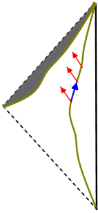
Figure 6:

We have shown that the effective modes associated with thermofield-double in one and two dimensions are the reparametrization modes (see [23]). On the other hand, such modes are specific to one and two dimensions. Therefore, a natural question that one can ask is, “What about higher dimensions?” First, it is important to emphasize that our argument for the existence of TFD’s effective modes on the physical boundary in the introduction 1 is right for any dimensions. Second, One should notice that the structure of two-point functions at finite temperature is not determined by symmetries for $d>2$ as $S^{1}\times\mathds{R}^{d-1}$ is not conformally equivalent to $\mathds{R}^{d}$; see [51] and references therein for more detail. This means that finite temperature two-point functions and higher point functions must have more sophisticated structures, and the TFD’s effective degrees of freedom and the corresponding action describing their dynamics as a result.

What happens if we go instead along the second time direction deep into the bulk? More precisely, do the metric fluctuations on the boundary lead to any nontrivial physics in the bulk? While this is a work in progress[52], we would like to say a few words about it. The key point here is that while the bulk always satisfies vacuum Einstein’s equation, the value of the Brown-York stress tensor is a function of these fluctuations. The ADM mass and angular momentum or, equivalently, the expectation value of the Hamiltonian and angular momentum operators are associated with the physical hypersurface that is the solution to the equation of motion of the GHY action. From the bulk point of view, this hypersurface corresponds to the event horizon. What about the off-shell values of the Brown-York tensor? A natural candidate is the associated focal hypersurface in the bulk, which is schematically drawn in figure 6. Moreover, the causal direction $\partial_{r}$ toward deep into the bulk can be regarded as the direction that boundary fluctuations propagate to reach the horizon . We are mostly interested in studying the horizon fluctuation in the second scheme. Note that there are also other candidates for the off-shell horizon, and we are going to study them in the upcoming paper [52].

Acknowledgment   I am grateful to John Preskill for helpful discussions and especially to Alexei Kitaev for helpful discussions and advice at different stages of this project. This work is supported by Simons Foundation, as well as by the Institute of Quantum Information and Matter, the NSF Frontier center funded in part by the Gordon and Betty Moore Foundation.

Appendix A Derivation of the metric

In this section, we will address the general form of the metric in our gauge choice. Unfortunately, as opposed to the FG gauge, where Einstein’s equation takes a simple form, our derivation is tedious.
Einstein equation

$$R_{\mu\nu}-\frac{1}{2}Rg_{\mu\nu}+\Lambda g_{\mu\nu}=0$$ (A.137)

in three dimensions where the Weyl tensor vanishes identically, can be rewritten in terms of the Riemann tensor:

$$R_{\mu\nu\rho\sigma}=\Lambda\Big{(}g_{\mu\rho}g_{\nu\sigma}-g_{\mu\sigma}g_{\nu\rho}\Big{)},$$ (A.138)

where the Riemann tensor has the following form

$$R_{\mu\nu\rho\sigma}\equiv\frac{1}{2}\Big{(}\partial_{\rho}\partial_{\nu}g_{\mu\sigma}+\partial_{\mu}\partial_{\sigma}g_{\rho\nu}-\partial_{\mu}\partial_{\rho}g_{\nu\sigma}-\partial_{\nu}\partial_{\sigma}g_{\mu\rho}\Big{)}+g_{\gamma\delta}\Big{(}\Gamma^{\gamma}_{\nu\rho}\Gamma^{\delta}_{\mu\sigma}-\Gamma^{\gamma}_{\mu\rho}\Gamma^{\delta}_{\nu\sigma}\Big{)}$$ (A.139)

From now on, we take $\Lambda=-1$. Consider the following ansatz for the metric

$$ds^{2}=g_{rv}~{}drdv+g_{ru}~{}drdu+g_{ij}(r,u,v)~{}dx^{i}dx^{j}$$ (A.140)

$$g_{ij}(r,x)=\frac{h^{(0)}_{ij}(x)}{r^{2}}+\frac{h^{(1)}_{ij}(x)}{r}+h^{(2)}_{ij}(x)+\cdots,~{}~{}~{}~{}~{}g_{ri}=\frac{h_{ri}(x)}{r^{2}}$$

In other words, we assume $g_{rr}\equiv 0$, and $h_{ru},h_{rv}$ are not functions of $r$. First consider $R_{rirj}$. from A.138 and A.139 we have

$$g_{ij}^{\prime\prime}=-2g_{ir}g_{rj}+2g_{\mu\nu}\Gamma^{\mu}_{ir}\Gamma^{\nu}_{rj}-\frac{2}{r}g^{\prime}_{ij}.$$ (A.141)

Here, the derivative is with respect to $r$. Using this expression for $g^{\prime\prime}_{ij}$, we have:

$$(r^{2}g_{ij})^{\prime\prime\prime}=8rg_{\mu\nu}\Gamma^{\mu}_{ir}\Gamma^{\nu}_{rj}+2r^{2}\Big{(}g_{\mu\nu}\Gamma^{\mu}_{ir}\Gamma^{\nu}_{rj}\Big{)}^{\prime}$$ (A.142)

To show the r.h.s is in fact, zero, we will compute the second term and use A.141 again. After manipulations, it will take the following form:

$$\Big{(}g_{\mu\nu}\Gamma^{\mu}_{ir}\Gamma^{\nu}_{rj}\Big{)}^{\prime}=-\frac{4}{r}\,g_{mn}\Gamma^{m}_{ir}\Gamma^{n}_{rj}+g_{pq}\Big{(}\Gamma^{m}_{jr}\Gamma^{p}_{ir}\Gamma^{q}_{mr}+(i\leftrightarrow j)\Big{)}-g^{\prime}_{mn}\Gamma^{m}_{ir}\Gamma^{n}_{jr}=-\frac{4}{r}g_{mn}\Gamma^{m}_{ir}\Gamma^{n}_{rj}$$ (A.143)

where the last equality can be seen by expanding the three Christoffel symbols in the middle equation. Plugging back into A.142 yields:

$$\Big{(}r^{2}g_{ij}\Big{)}^{\prime\prime\prime}=0$$ (A.144)

On the other hand, Einstein’s equation at leading order implies that $g^{rr}=r^{2}+O(r)$, which means the boundary $\mathcal{I}$ of $\widetilde{M}$ is time-like. This can be easily seen, for example, by rewriting A.138 on $\widetilde{M}$ in terms of $\widetilde{g}_{\mu\nu}$. To simplify the computation, we further choose the conformal gauge for the transverse direction to the leading order. Then, $g^{rr}=r^{2}$ implies that $-2h_{ru}h_{rv}=h_{uv}$. Using A.142, we can write the metric components as follows:

$$g_{rr}=0,~{}~{}~{}~{}g_{ru}=-\frac{e^{\varphi_{1}}}{2r^{2}},~{}~{}~{}~{}g_{rv}=-\frac{e^{\varphi_{2}}}{2r^{2}},~{}~{}~{}~{}g_{uv}=-\frac{e^{\varphi_{1}+\varphi_{2}}}{2r^{2}}+\frac{h^{(1)}_{uv}}{2r}+h^{(0)}_{uv},$$ (A.145)

$$g_{vv}=\frac{h^{(1)}_{vv}}{r}+h^{(0)}_{vv},~{}~{}~{}~{}g_{ww}=\frac{h^{(1)}_{ww}}{r}+h^{(0)}_{ww}$$

To study Einstein’s equation to next orders, we found it relatively simpler to study $R^{\mu}_{~{}\nu\rho\sigma}=-\Big{(}g^{\mu}_{~{}\rho}~{}g_{\nu\sigma}-g^{\mu}_{~{}\sigma}\,g_{\nu\rho}\Big{)}.$ $R^{v}_{~{}uru}=~{}R^{u}_{~{}vrv}=0$ implies:

$$\boxed{h^{(1)}_{uu}=e^{\varphi_{1}}\partial_{u}\varphi_{2},~{}~{}~{}~{}~{}~{}~{}h_{vv}^{(1)}=e^{\varphi_{2}}\partial_{v}\varphi_{1}}$$ (A.146)

However, $h^{(1)}_{uv}$ remains undetermined. In the next order, Einstein’s equation leads to only one constraint which can be used to determine, say, $h^{(0)}_{uv}$ as a function of $h^{(0)}_{uu}$ and $h^{(0)}_{vv}$:

$$h^{(0)}_{uv}=e^{-\varphi_{1}-\varphi_{2}}\Big{(}e^{2\varphi_{1}}\,h^{(0)}_{vv}+e^{2\varphi_{2}}\,h^{(0)}_{uu}-\frac{1}{4}(-h^{(1)}_{uv}+\partial_{u}e^{\varphi_{2}}+\partial_{v}e^{\varphi_{1}})^{2}\Big{)}$$ (A.147)

The easiest way to see this is by studying $R^{i}_{~{}rir}=0$ at $O\,(\Omega^{0})$. Now, to derive an expression for $h^{(0)}_{uu}$ and $h^{(0)}_{vv}$ we need to study the Einstein’s equation at $O(\Omega^{1})$. Einstein’s equation associated with $R^{v}_{~{}vuv}$ and $R^{u}_{~{}uvu}$ yields a first order differential equation for $h^{(0)}_{uu}$ and $h^{(0)}_{vv}$, namely:

$$\partial_{v}h^{(0)}_{uu}=\frac{1}{2}\partial_{v}\bigg{[}\frac{1}{2}\partial_{u}\varphi^{2}_{2}-\frac{1}{2}\partial_{u}\varphi^{2}_{1}+e^{-\varphi_{2}}\Big{(}-\partial_{u}h^{(1)}_{uv}+h^{(1)}_{uv}\partial_{v}\varphi_{1}\Big{)}+\partial_{u}^{2}\varphi_{1}+e^{\varphi_{1}-\varphi_{2}}\partial_{u}\partial_{v}\varphi_{2}\bigg{]}$$ (A.148)

$$\partial_{u}h^{(0)}_{vv}=\frac{1}{2}\partial_{u}\bigg{[}\frac{1}{2}\partial_{u}\varphi^{2}_{1}-\frac{1}{2}\partial_{v}\varphi^{2}_{2}+e^{-\varphi_{1}}\Big{(}-\partial_{v}h^{(1)}_{uv}+h^{(1)}_{uv}\partial_{v}\varphi_{2}\Big{)}+\partial_{v}^{2}\varphi_{2}+e^{\varphi_{2}-\varphi_{1}}\partial_{u}\partial_{v}\varphi_{1}\bigg{]}$$

whose solution determine $h^{(0)}_{uu}$ and $h^{(0)}_{vv}$ up to a chiral and anti-chiral functions $A(u)$ and $B(v)$, respectively:

$$\boxed{\begin{aligned} &h^{(0)}_{uu}=\frac{1}{2}\bigg{[}\frac{1}{2}\partial_{u}\varphi^{2}_{2}-\frac{1}{2}\partial_{u}\varphi^{2}_{1}+e^{-\varphi_{2}}\Big{(}-\partial_{u}h^{(1)}_{uv}+h^{(1)}_{uv}\partial_{u}\varphi_{1}\Big{)}+\partial_{u}^{2}\varphi_{1}+e^{\varphi_{1}-\varphi_{2}}\partial_{u}\partial_{v}\varphi_{2}\bigg{]}+\frac{g^{(0)}_{uu}(u)}{2}\\ &h^{(0)}_{vv}=\frac{1}{2}\bigg{[}\frac{1}{2}\partial_{v}\varphi^{2}_{1}-\frac{1}{2}\partial_{v}\varphi^{2}_{2}+e^{-\varphi_{1}}\Big{(}-\partial_{v}h^{(1)}_{uv}+h^{(1)}_{uv}\partial_{v}\varphi_{2}\Big{)}+\partial_{v}^{2}\varphi_{2}+e^{\varphi_{2}-\varphi_{1}}\partial_{u}\partial_{v}\varphi_{1}\bigg{]}+\frac{g^{(0)}_{vv}(v)}{2}\end{aligned}}$$ (A.149)

The metric components A.145 with 2.43,  A.147, and A.149 are, in fact, the exact solution to Einstein’s equation. The determinant of the transverse metric is:

$$\sqrt{-\det g_{ij}}=\frac{e^{\varphi_{1}+\varphi_{2}}}{2r^{2}}-\frac{h^{(1)}_{uv}}{2r}+\frac{1}{8}e^{-\varphi_{1}-\varphi_{2}}(h^{(1)}_{uv})^{2}+\frac{1}{4}e^{-\varphi_{1}}\Big{(}\partial_{u}h^{(1)}_{uv}-h^{(1)}_{uv}\partial_{u}(\varphi_{1}+\varphi_{2})\Big{)}$$ (A.150)

$$+\frac{1}{4}e^{-\varphi_{2}}\Big{(}\partial_{v}h^{(1)}_{uv}-h^{(1)}_{uv}\partial_{v}(\varphi_{1}+\varphi_{2})\Big{)}+\frac{1}{8}e^{\varphi_{2}-\varphi_{1}}\Big{(}-2A(u)+\partial_{u}\varphi_{1}^{2}-2\partial_{u}^{2}\varphi_{1}\Big{)}$$

$$+\frac{1}{8}e^{\varphi_{1}-\varphi_{2}}\Big{(}-2B(v)+\partial_{v}\varphi_{2}^{2}-2\partial_{v}^{2}\varphi_{2}\Big{)}-\frac{1}{4}\bigg{(}3\,\partial_{u}\varphi_{2}\partial_{v}\varphi_{1}+\partial_{u}\partial_{v}\Big{(}\varphi_{1}+\varphi_{2}\Big{)}\bigg{)}+O(r)$$

Plugging the above into the GHY action over the hypersurface $r=\varepsilon$ and using 2.36, the action will take the following form:

$$S_{GHY}=\int~{}dudv~{}\Bigg{[}\frac{e^{\varphi_{1}+\varphi_{2}}}{2\varepsilon^{2}}-\frac{h^{(1)}_{uv}}{2\varepsilon}+\frac{1}{8}e^{-\varphi_{1}-\varphi_{2}}(h^{(1)}_{uv})^{2}-\frac{1}{4}e^{-\varphi_{1}}h^{(1)}_{uv}\partial_{u}\varphi_{2}-\frac{1}{4}e^{-\varphi_{2}}h^{(1)}_{uv}\partial_{v}\varphi_{1}\Big{)}$$ (A.151)

$$~{}~{}+\frac{1}{8}e^{\varphi_{2}-\varphi_{1}}\Big{(}-2A(u)+\partial_{u}\varphi_{1}^{2}-2\partial_{u}^{2}\varphi_{1}\Big{)}+\frac{1}{8}e^{\varphi_{1}-\varphi_{2}}\Big{(}-2B(v)+\partial_{v}\varphi_{2}^{2}-2\partial_{v}^{2}\varphi_{2}\Big{)}\,-\frac{3}{4}\partial_{u}\varphi_{2}\partial_{v}\varphi_{1}+O(\varepsilon)\Bigg{]},$$

$$O(\varepsilon)=\frac{1}{2}e^{-\varphi_{1}-\varphi_{2}}\bigg{(}\partial_{v}h^{(1)}_{uv}\partial_{u}\varphi_{2}+\partial_{u}h^{(1)}_{uv}\partial_{v}\varphi_{1}-h^{(1)}_{uv}\Big{(}\partial_{v}\phi_{1}\partial_{u}\varphi_{1}+\partial_{v}\phi_{2}\partial_{u}\varphi_{2}+2\partial_{u}\varphi_{2}\partial_{v}\varphi_{1}\Big{)}\bigg{)}\varepsilon+\cdots$$

Appendix B Computation of the two-point function

B.1 The $SL(2,R)_{L}\times SL(2,R)_{R}$ shockwaves

In this section, we will compute the OTOCs associated with the left-handed and right-handed modes. From the bulk point of view, they correspond to the scattering of shock waves associated with the left (right) ingoing and outgoing modes. However, their nature is non-gravitational; They correspond to the $SL(2,R)$ transformations that move the bifurcation horizon [52]. To compute the related amplitudes, we will closely follow [18]. We consider a solution on the boundary where in the absence of any perturbation $U_{-}^{(0)}=e^{u}$. Now we will add the effect of the first perturbation, which takes $U_{-}^{(0)}$ to

$$U_{-}^{(1)}=e^{\frac{2\pi u}{\beta_{+}}}+X_{-}$$ (B.152)

or equivalently, if we define $x=\tanh\frac{\pi u}{\beta_{+}}$

$$U_{-}^{(0)}=x~{}~{}~{}\rightarrow~{}~{}~{}U_{-}^{(1)}=U_{-}^{(0)}+\frac{(1-x)^{2}X_{-}}{2+(1-x)X_{-}}$$ (B.153)

The second perturbation corresponds to:

$$U_{-}^{(0)}=x~{}~{}~{}\rightarrow~{}~{}~{}U_{-}^{(1)}=U_{-}^{(0)}-\frac{(1+x)^{2}X_{+}}{2+(1+x)X_{+}}$$ (B.154)

We are interested in the superposition of the two solutions, namely,

$$U_{-}=U_{-}^{(0)}+\frac{(1-x)^{2}X_{-}}{2+(1-x)X_{-}}-\frac{(1+x)^{2}X_{+}}{2+(1+x)X_{+}}$$ (B.155)

The value of the Schwarzian action associated with the above off-shell solution is:

$$\frac{i}{8G}\int_{-\infty}^{\infty}du~{}\operatorname{Sch}(U_{-},u)=\frac{i\pi}{2\beta_{+}G}X_{-}X_{+}\equiv i\,\frac{S_{+}}{\pi}X_{-}X_{+}$$ (B.156)

The same computation, but this time for $U_{+}$ direction

$$U_{+}=U_{+}^{(0)}+\frac{(1-y)^{2}Y_{-}}{2+(1-y)Y_{-}}-\frac{(1+y)^{2}Y_{+}}{2+(1+y)Y_{+}},~{}~{}~{}~{}~{}~{}y=\tanh\frac{v}{2}$$ (B.157)

yields the following result:

$$\frac{i}{8G}\int_{-\infty}^{\infty}dv~{}\operatorname{Sch}(U_{+},v)=\frac{i\pi}{2\beta_{-}G}Y_{-}Y_{+}\equiv i\frac{S_{-}}{\pi}\,Y_{-}Y_{+}$$ (B.158)

Now, under the perturbation, the two-point function will deform to:

$$\widetilde{G}(u_{1}^{(m)},u^{(n)}_{2})\approx\frac{b}{\bigg{(}\frac{\beta_{+}J}{\pi}\Big{(}2\sinh\frac{\pi(u^{(m)}_{1}-u^{(n)}_{2})}{\beta_{+}}-X_{-}e^{-\frac{\pi}{\beta_{+}}(u^{(m)}_{1}+u^{(n)}_{2})}\Big{)}\bigg{)}^{2\Delta_{1}}}$$ (B.159)

$$~{}~{}~{}~{}~{}~{}~{}~{}~{}~{}~{}~{}~{}~{}~{}~{}=G(u_{1}^{(m)},u_{2}^{(n)})~{}~{}\frac{1}{\Big{(}1-\frac{e^{-\frac{\pi}{\beta_{+}}(u^{(m)}_{1}+u^{(n)}_{2})}}{2\sinh\frac{\pi}{\beta_{+}}(u_{1}^{(m)}-u_{2}^{(n)})}X_{-}\Big{)}^{2\Delta_{1}}}$$

$$\widetilde{G}(u_{3}^{(p)},u^{(q)}_{4})\approx\frac{b}{\bigg{(}\frac{\beta_{+}J}{\pi}\Big{(}2\sinh\frac{\pi(u^{(p)}_{3}-u^{(q)}_{4})}{\beta_{+}}-X_{+}e^{\frac{\pi}{\beta_{+}}(u^{(p)}_{3}+u^{(q)}_{4})}\Big{)}\bigg{)}^{2\Delta_{2}}}$$

$$~{}~{}~{}~{}~{}~{}~{}~{}~{}~{}~{}~{}~{}~{}~{}=G(u_{3}^{(p)},u^{(q)}_{4})~{}~{}\frac{1}{\Big{(}1-\frac{e^{\frac{\pi}{\beta_{+}}(u^{(p)}_{3}+u^{(q)}_{4})}}{2\sinh\frac{\pi}{\beta_{+}}(u_{3}^{(p)}-u_{4}^{(q)})}X_{+}\Big{)}^{2\Delta_{2}}}$$

To compute the OTOC we have [18]:

$$\int~{}dX_{+}dX_{-}~{}e^{-i\frac{S_{+}}{\pi}X_{+}X_{-}}~{}\widetilde{G}(u_{1}^{(m)},u^{(n)}_{2})\,\,\widetilde{G}(u_{3}^{(p)},u^{(q)}_{4})$$ (B.160)

$$\propto G(u_{1}^{(m)},u_{2}^{(n)})G(u_{3}^{(p)},u^{(q)}_{4})\times(iC_{mnpq})^{-2\Delta_{1}}U(2\Delta_{1},1-2\Delta_{2}+2\Delta_{1},\frac{1}{iC_{mnpq}}),$$

$$~{}~{}~{}~{}~{}~{}~{}C_{mnpq}=\frac{\pi}{S}~{}\frac{e^{\frac{\pi}{\beta_{+}}(u^{(p)}_{3}+u^{(q)}_{4}-u^{(n)}_{1}-u^{(m)}_{2})}}{4\sinh\frac{\pi}{\beta_{+}}(u^{(n)}_{1}-u^{(m)}_{2})\sinh\frac{\pi}{\beta_{+}}(u^{(p)}_{3}-u^{(q)}_{4})}$$

By checking with OTOC in the short time we can fix the overall coefficient. Consequently, we will get the following expression for the OTOC:

$$\bigg{\langle}\frac{\delta G(u_{1}^{(m)},u_{2}^{(n)})}{G(u_{1}^{(m)},u_{2}^{(n)})}\frac{\delta G(u_{3}^{(p)},u^{(q)}_{4})}{G(u_{3}^{(p)},u^{(q)}_{4})}\bigg{\rangle}=(iC_{mnpq})^{-2\Delta_{1}}U(2\Delta_{1},1-2\Delta_{2}+2\Delta_{1},\frac{1}{iC_{mnpq}}).$$ (B.161)

B.2 The deformed two-point function

$$\widetilde{G}(t_{2},\phi_{2};t_{1},\phi_{1})=\Big{\langle}\widetilde{TFD}\Big{|}\,\mathcal{O}(t_{2},\phi_{2})\mathcal{O}(t_{1},\phi_{1})\Big{|}\widetilde{TFD}\Big{\rangle}=\Big{\langle}\,\mathcal{O}(it_{2},\phi_{2})\mathcal{O}(it_{1},\phi_{1})\Big{\rangle}$$ (B.162)

$$-ig\int_{0}^{2\pi}~{}d\phi~{}\Bigg{[}\int_{t_{0}}^{t_{1}}~{}du~{}\Big{\langle}\mathcal{O}(it_{2},\phi_{2})\mathcal{O}(it_{1},\phi_{1})O_{R}(iu,\phi)O_{L}(-iu,\phi)\Big{\rangle}$$

$$-\int_{t_{0}}^{t_{2}}du\Big{\langle}O_{R}(iu,\phi)O_{L}(-iu,\phi)\mathcal{O}(it_{2},\phi_{2})\mathcal{O}(it_{1},\phi_{1})\Big{\rangle}$$

$$+\int_{t_{1}}^{t_{2}}du\Big{\langle}\mathcal{O}(it_{2},\phi_{2})O_{R}(iu,\phi)O_{L}(-iu,\phi)\mathcal{O}(it_{1},\phi_{1})\Big{\rangle}\Bigg{]}\equiv A+B$$

$$A=\sum_{m}G_{m}(iu_{21},iv_{21})\times$$

$$\Bigg{[}1-2\pi ig~{}\mathcal{F}_{m}(iu_{21})\sum_{n}\bigg{(}\int_{t_{0}}^{t_{1}}du\,\,G_{n}(2iu+\frac{\beta_{+}}{2},2iu+\frac{\beta_{-}}{2})\,\,\bigg{[}\mathcal{F}_{n}(2iu+\frac{\beta_{+}}{2})-\mathcal{F}_{n}(-2iu+\frac{\beta_{+}}{2})\bigg{]}\bigg{)}$$

$$~{}~{}~{}-2\pi ig~{}\mathcal{F}_{m}(iv_{12})\sum_{n}\bigg{(}\int_{t_{0}}^{t_{1}}du\,\,G_{n}(2iu+\frac{\beta_{+}}{2},2iu+\frac{\beta_{-}}{2})\,\,\bigg{[}\mathcal{F}_{n}(2iu+\frac{\beta_{-}}{2})-\mathcal{F}_{n}(-2iu+\frac{\beta_{-}}{2})\bigg{]}\bigg{)}\Bigg{]}$$

$$B=\int_{t_{1}}^{t_{2}}~{}du~{}\Bigg{[}-\sum_{n,m}G_{m}(iu_{12},iv_{12})\bigg{[}2\pi ig\mathcal{F}_{m}(iu_{21})G_{n}(-2iu+\frac{\beta_{+}}{2},,-2iu+\frac{\beta_{-}}{2})\,\,\mathcal{F}_{n}(-2iu+\frac{\beta_{+}}{2})$$

$$~{}~{}~{}~{}~{}~{}~{}~{}~{}~{}~{}~{}~{}~{}+2\pi ig\mathcal{F}_{m}(iv_{21})G_{n}(-2iu+\frac{\beta_{+}}{2},,-2iu+\frac{\beta_{-}}{2})\,\,\mathcal{F}_{n}(-2iu+\frac{\beta_{-}}{2})\bigg{]}$$

$$~{}~{}~{}~{}~{}~{}~{}~{}~{}~{}~{}~{}~{}~{}-2\pi ig\bigg{(}\Big{\langle}\mathcal{O}(it_{2},\phi_{2})O_{R}(iu,\phi)O_{L}(-iu,\phi)\mathcal{O}(it_{1},\phi_{1})\Big{\rangle}-G(iu_{21},iv_{21})G(2iu+\frac{\beta_{+}}{2},2iu+\frac{\beta_{-}}{2})\bigg{)}\Bigg{]}$$

Here A and B are, roughly speaking, the equilibrium and non-equilibrium parts. More precisely, computing A leads to 4.122. Now, we would like to show that for $t_{1}$ sufficiently bigger than $\beta_{+}$, $B$ will be negligible. First, we will use the following estimation for the two-point function,

$$G(2iu+\frac{\beta_{+}}{2},2iu+\frac{\beta_{-}}{2})\sim\sum_{n=-\infty}^{\infty}~{}\frac{1}{\Big{(}\cosh(\frac{2\pi u}{\beta_{+}}-\frac{2\pi^{2}n}{\beta_{+}})\Big{)}^{2\Delta_{+}}}\frac{1}{\Big{(}\cosh(\frac{2\pi u}{\beta_{-}}+\frac{2\pi^{2}n}{\beta_{-}})\Big{)}^{2\Delta_{-}}}$$ (B.163)

$$~{}~{}~{}~{}~{}~{}~{}~{}~{}~{}~{}~{}~{}~{}~{}~{}~{}~{}~{}~{}~{}~{}~{}~{}~{}~{}~{}~{}~{}~{}~{}~{}~{}~{}~{}~{}~{}\leq\frac{e^{-\frac{4\pi\Delta_{-}t_{1}}{\beta_{-}}}}{1-e^{-\frac{4\pi^{2}\Delta_{-}}{\beta_{-}}}}+\frac{e^{-\frac{4\pi\Delta_{+}t_{1}}{\beta_{+}}}}{1-e^{-\frac{4\pi^{2}\Delta_{+}}{\beta_{+}}}}$$

Second, we can rewrite $B$ as follows:

$$\sum_{n}~{}G_{n}(-2iu+\frac{\beta_{+}}{2},-2iu+\frac{\beta_{-}}{2})\,\mathcal{F}_{n}(-2iu+\frac{\beta_{+}}{2})\sim$$ (B.164)

$$\sum_{n=-\infty}^{\infty}\bigg{|}~{}\frac{(1-\frac{2\pi u^{(n)}}{\beta_{+}}+\frac{i\pi}{2})\tanh\frac{2\pi u^{(n)}}{\beta_{+}}}{\Big{(}\cosh(\frac{2\pi u}{\beta_{+}}-\frac{2\pi^{2}n}{\beta_{+}})\Big{)}^{2\Delta_{+}}}\frac{1}{\Big{(}\cosh(\frac{2\pi u}{\beta_{-}}+\frac{2\pi^{2}n}{\beta_{-}})\Big{)}^{2\Delta_{-}}}\bigg{|}\leq(1+\frac{\pi}{2})\Big{|}G(2iu+\frac{\beta_{+}}{2},2iu+\frac{\beta_{-}}{2})\Big{|}$$

$$~{}~{}~{}~{}~{}~{}~{}~{}~{}~{}~{}~{}+\Bigg{(}\frac{2\pi}{\beta_{+}}\frac{e^{-8\pi^{2}\frac{\Delta_{+}}{\beta_{+}}}(\pi-u(1-e^{4\pi^{2}\frac{\Delta_{+}}{\beta_{+}}}))}{(1-e^{4\pi^{2}\frac{\Delta_{+}}{\beta_{+}}})^{2}}\Bigg{)}e^{-4\pi\Delta_{+}\frac{u}{\beta_{+}}}+\Bigg{(}O(u)+O(e^{-4\pi\Delta_{+}\frac{n_{0}\pi-u}{\beta_{+}}})\Bigg{)}e^{-4\pi\Delta_{-}\frac{u}{\beta_{-}}},$$

where we assumed $(n_{0}-1)\pi<u<n_{0}\pi$. To estimate the OTOC, First, we will use the following integral representation of the confluent hypergeometric function:

$$U(2\Delta_{1},1-2(\Delta_{2}-\Delta_{1}),-i|z|)=\frac{(-i)^{2\Delta_{1}-1}}{\Gamma(2\Delta_{1})}\int_{0}^{\infty}~{}dt~{}e^{-|z|t}~{}~{}t^{2\Delta_{1}-1}~{}~{}(1-it)^{-2\Delta_{2}}$$ (B.165)

$$\Rightarrow\Big{|}U(2\Delta_{1},1-2(\Delta_{2}-\Delta_{1}),-i|z|)\Big{|}\leq\frac{1}{\Gamma(2\Delta_{1})}\int_{0}^{\infty}~{}dt~{}e^{-|z|t}~{}~{}t^{2\Delta_{1}-1}~{}~{}(1+t^{2})^{-\Delta_{2}}$$

Clearly, the last integral is monotonically decreasing as $|z|$ increases. at $|z|\rightarrow\infty$ it reaches $|z|^{-2\Delta_{1}}$, and as $|z|\rightarrow 0$ it reaches a constant which we call it A that can be written in terms of gamma functions. Now, using 4.113 with:

$$C^{\pm}_{n,m,p,q}=\frac{-\pi}{S_{\pm}}\frac{e^{\frac{\pi}{\beta_{\pm}}(t_{1}+t_{2}+2\phi+\tilde{n}-\tilde{p})}}{\Big{(}\sinh\frac{\pi}{\beta_{\pm}}(u_{12}\pm\tilde{m})\Big{)}\Big{(}2\cosh\frac{\pi}{\beta_{\pm}}(2u\pm\tilde{q})\Big{)}},~{}~{}~{}~{}~{}\tilde{n}=\frac{n+m}{2},~{}~{}~{}~{}\tilde{m}=\frac{n-m}{2}$$ (B.166)

yields

$$0\lesssim\Big{|}\Big{(}iC^{\pm}_{m,n,p,q}\Big{)}^{-2\Delta_{\pm}}U\Big{(}2\Delta^{\pm}_{1},1-2(\Delta^{\pm}_{2}-\Delta^{\pm}_{1}),(iC_{m,n,p,q})^{-1}\Big{)}\Big{|}\lesssim A$$ (B.167)

Now, we can easily estimate the last line of B in B.162:

$$\bigg{|}\Big{\langle}\mathcal{O}(it_{2},\phi_{2})O_{R}(iu,\phi)O_{L}(-iu,\phi)\mathcal{O}(it_{1},\phi_{1})\Big{\rangle}-G(iu_{21},iv_{21})G(2iu+\frac{\beta_{+}}{2},2iu+\frac{\beta_{-}}{2})\bigg{|}$$ (B.168)

$$\sim AG(iu_{21},iv_{21})G(2iu+\frac{\beta_{+}}{2},2iu+\frac{\beta_{-}}{2})$$

Collecting all the estimations will imply that:

$$\Big{|}B\Big{|}=O(e^{\frac{-4\pi\Delta_{+}t_{1}}{\beta_{+}}},e^{-\frac{4\pi\Delta_{-}t_{1}}{\beta_{-}}})$$ (B.169)

References

- [1] J. M. Bardeen, B. Carter and S. W. Hawking, The four laws of black hole mechanics, Communications in Mathematical Physics 31 (Jun, 1973) 161–170.
- [2] W. Israel, Thermo field dynamics of black holes, Phys. Lett. A 57 (1976) 107–110.
- [3] G. ’t Hooft, Dimensional reduction in quantum gravity, gr-qc/9310026.
- [4] L. Susskind, The world as a hologram, J.Math.Phys. 36 (1995) 6377–6396, [hep-th/9409089].
- [5] M. V. Raamsdonk, Comments on quantum gravity and entanglement, 0907.2939.
- [6] J. Maldacena and L. Susskind, Cool horizons for entangled black holes, 1306.0533.
- [7] J. Maldacena, The large-n limit of superconformal field theories and supergravity, International Journal of Theoretical Physics 38 (Apr, 1999) 1113–1133.
- [8] E. Witten, Anti de sitter space and holography, Adv.Theor.Math.Phys. 2 (1998) 253–291, [hep-th/9802150].
- [9] S. S. Gubser, I. R. Klebanov and A. M. Polyakov, Gauge theory correlators from non-critical string theory, Phys.Lett.B 428 (1998) 105–114, [hep-th/9802109].
- [10] J. Maldacena, S. H. Shenker and D. Stanford, A bound on chaos, 1503.01409.
- [11] S. H. Shenker and D. Stanford, Black holes and the butterfly effect, 1306.0622.
- [12] S. H. Shenker and D. Stanford, Stringy effects in scrambling, 1412.6087.
- [13] S. Sachdev and J. Ye, Gapless spin-fluid ground state in a random quantum heisenberg magnet, Phys.Rev.Lett. 70 (1993) 3339, [cond-mat/9212030].
- [14] A. Kitaev and S. J. Suh, The soft mode in the sachdev-ye-kitaev model and its gravity dual, 1711.08467.
- [15] J. Maldacena and D. Stanford, Comments on the sachdev-ye-kitaev model, Phys. Rev. D 94 (2016) 106002, [1604.07818].
- [16] R. Jackiw, Lower Dimensional Gravity, Nucl. Phys. B 252 (1985) 343–356.
- [17] C. Teitelboim, Gravitation and Hamiltonian Structure in Two Space-Time Dimensions, Phys. Lett. B 126 (1983) 41–45.
- [18] J. Maldacena, D. Stanford and Z. Yang, Conformal symmetry and its breaking in two dimensional nearly anti-de-sitter space, 1606.01857.
- [19] J. M. Maldacena, Eternal black holes in ads, JHEP 0304 (2003) 021, [hep-th/0106112].
- [20] P. Gao, D. L. Jafferis and A. C. Wall, Traversable wormholes via a double trace deformation, 1608.05687.
- [21] J. Maldacena and X.-L. Qi, Eternal traversable wormhole, 1804.00491.
- [22] Y. Chen and P. Zhang, Entanglement entropy of two coupled syk models and eternal traversable wormhole, 1903.10532.
- [23] P. Dadras, Disentangling the thermofield-double state, Journal of High Energy Physics 2022 (Jan, 2022) 75.
- [24] E. Witten, (2+1)-Dimensional Gravity as an Exactly Soluble System, Nucl. Phys. B 311 (1988) 46.
- [25] E. Witten, Three-dimensional gravity revisited, 0706.3359.
- [26] J. D. Brown and M. Henneaux, Central Charges in the Canonical Realization of Asymptotic Symmetries: An Example from Three-Dimensional Gravity, Commun. Math. Phys. 104 (1986) 207–226.
- [27] M. Bañados, C. Teitelboim and J. Zanelli, The black hole in three dimensional space time, Phys.Rev.Lett. 69 (1992) 1849–1851, [hep-th/9204099].
- [28] M. Banados, M. Henneaux, C. Teitelboim and J. Zanelli, Geometry of the 2+1 black hole, Phys.Rev.D 48 (1993) 1506–1525, [gr-qc/9302012].
- [29] S. Carlip, Quantum Gravity in 2+1 Dimensions. Cambridge University Press, jul, 1998, 10.1017/cbo9780511564192.
- [30] G. W. Gibbons and S. W. Hawking, Action Integrals and Partition Functions in Quantum Gravity, Phys. Rev. D 15 (1977) 2752–2756.
- [31] S. W. Hawking and D. N. Page, Thermodynamics of black holes in anti-de sitter space, Communications in Mathematical Physics 87 (Dec, 1983) 577–588.
- [32] A. Maloney and E. Witten, Quantum gravity partition functions in three dimensions, JHEP 1002 (2010) 029, [0712.0155].
- [33] C. R. Fefferman, Charles; Graham, Conformal invariants, in élie cartan et les mathématiques d’aujourd’hui, Astérisque (Juin, 1984) .
- [34] K. Skenderis and S. N. Solodukhin, Quantum effective action from the ads/cft correspondence, Phys.Lett.B 472 (2000) 316–322, [hep-th/9910023].
- [35] S. de Haro, K. Skenderis and S. N. Solodukhin, Holographic reconstruction of spacetime and renormalization in the ads/cft correspondence, Commun.Math.Phys. 217 (2001) 595–622, [hep-th/0002230].
- [36] K. Skenderis, Lecture notes on holographic renormalization, Class.Quant.Grav. 19 (2002) 5849–5876, [hep-th/0209067].
- [37] A. Polyakov, Quantum geometry of bosonic strings, Physics Letters B 103 (1981) 207–210.
- [38] A. Polyakov, Quantum gravity in two dimensions, Mod. Phys. Lett. A 2 (1987) 893–898.
- [39] A. Ashtekar and S. Das, Asymptotically anti-de sitter space-times: Conserved quantities, Class.Quant.Grav. 17 (2000) L17–L30, [hep-th/9911230].
- [40] A. Ashtekar and A. Magnon, Asymptotically anti-de sitter space-times, Classical and Quantum Gravity 1 (jul, 1984) L39–L44.
- [41] J. D. Brown and J. W. York, Jr., Quasilocal energy and conserved charges derived from the gravitational action, Phys. Rev. D 47 (1993) 1407–1419, [gr-qc/9209012].
- [42] V. Balasubramanian and P. Kraus, A stress tensor for anti-de sitter gravity, Commun.Math.Phys. 208 (1999) 413–428, [hep-th/9902121].
- [43] H. Verlinde, Conformal field theory, two-dimensional quantum gravity and quantization of teichmüller space, Nuclear Physics B 337 (1990) 652–680.
- [44] A. Alekseev and S. Shatashvili, Path integral quantization of the coadjoint orbits of the virasoro group and 2-d gravity, Nuclear Physics B 323 (1989) 719–733.
- [45] J. Cotler and K. Jensen, A theory of reparameterizations for ads3 gravity, Journal of High Energy Physics 2019 (Feb, 2019) 79.
- [46] O. Coussaert, M. Henneaux and P. van Driel, The asymptotic dynamics of three-dimensional einstein gravity with a negative cosmological constant, Class.Quant.Grav. 12 (1995) 2961–2966, [gr-qc/9506019].
- [47] S. Carlip, Dynamics of asymptotic diffeomorphisms in (2+1)-dimensional gravity, Class. Quant. Grav. 22 (2005) 3055–3060, [gr-qc/0501033].
- [48] E. Keski-Vakkuri, Bulk and boundary dynamics in btz black holes, Phys. Rev. D 59 (1999) 104001, [hep-th/9808037].
- [49] H. T. Lam, T. G. Mertens, G. J. Turiaci and H. Verlinde, Shockwave s-matrix from schwarzian quantum mechanics, JHEP 1811 (2018) 182, [1804.09834].
- [50] A. Strominger, Black hole entropy from near-horizon microstates, JHEP 9802 (1998) 009, [hep-th/9712251].
- [51] L. Iliesiu, M. Koloğlu, R. Mahajan, E. Perlmutter and D. Simmons-Duffin, The conformal bootstrap at finite temperature, 1802.10266.
- [52] Work in progress, .