Parameterized Complexity of Chordal Conversion for
Sparse Semidefinite Programs with Small Treewidth

Abstract

If a sparse semidefinite program (SDP), specified over $n\times n$ matrices and subject to $m$ linear constraints, has an aggregate sparsity graph $G$ with small treewidth, then chordal conversion will frequently allow an interior-point method to solve the SDP in just $O(m+n)$ time per-iteration. This is a significant reduction over the minimum $\Omega(n^{3})$ time per-iteration for a direct solution, but a definitive theoretical explanation was previously unknown. Contrary to popular belief, the speedup is not guaranteed by a small treewidth in $G$, as a diagonal SDP would have treewidth zero but can still necessitate up to $\Omega(n^{3})$ time per-iteration. Instead, we construct an extended aggregate sparsity graph $\overline{G}\supseteq G$ by forcing each constraint matrix $A_{i}$ to be its own clique in $G$. We prove that a small treewidth in $\overline{G}$ does indeed guarantee that chordal conversion will solve the SDP in $O(m+n)$ time per-iteration, to $\epsilon$-accuracy in at most $O(\sqrt{m+n}\log(1/\epsilon))$ iterations. For classical SDPs like the MAX-$k$-CUT relaxation and the Lovasz Theta problem, the two sparsity graphs coincide $G=\overline{G}$, so our result provide a complete characterization for the complexity of chordal conversion, showing that a small treewidth is both necessary and sufficient for $O(m+n)$ time per-iteration. Real-world SDPs like the AC optimal power flow relaxation have different graphs $G\subseteq\overline{G}$ with similar small treewidths; while chordal conversion is already widely used on a heuristic basis, in this paper we provide the first rigorous guarantee that it solves such SDPs in $O(m+n)$ time per-iteration.
[We solve a Lovasz Theta problem with $n=10^{6}$ and $m=1.5\times 10^{6}$ in just 30 minutes, and an AC optimal power flow relaxation with $n=8.2\times 10^{4}$ and $m\approx 2.5\times 10^{5}$ in less than 4 hours, on a modest workstation using a MATLAB implementation and the MOSEK solver. See supporting code at https://github.com/ryz-codes/chordalConv/]

1 Introduction

We wish to solve the following standard-form semidefinite program to high accuracy:

$$\min_{X\in\mathbb{S}^{n}}\;\left\langle C,X\right\rangle\quad\text{s.t.}\;X\succeq 0,\quad\left\langle A_{i},X\right\rangle\leq b_{i}\;\text{for all }i\in\{1,2,\dots,m\}.$$ (SDP)

Here, $\mathbb{S}^{n}$ denotes the set of $n\times n$ real symmetric matrices with inner product $\left\langle A_{i},X\right\rangle=\operatorname{tr}(A_{i}^{T}X)$, and $X\succeq 0$ to means that $X$ is positive semidefinite. The problem data are the objective matrix $C\in\mathbb{S}^{n}$, constraint matrices $A_{1},\dots,A_{m}\in\mathbb{S}^{n}$ and bounds $b_{1},\dots,b_{m}\in\mathbb{R}$; we will assume that $C,A_{1},\dots,A_{m}$ are sparse matrices.

Our demand for high accuracy motivates us to consider interior-point methods; general-purpose implementations, such as SeDuMi [57], SDPT3 [64], and MOSEK [46], often attain accuracies of $\epsilon\approx 10^{-8}$ in just tens of iterations. However, their potentially high per-iteration cost is a major concern. A direct application of a general-purpose solver to (SDP) results in a per-iteration cost of at least $\Omega(n^{3})$, and this in practice limits the value of $n$ to no more than a few thousand.

Instead, to handle $n$ as large as a hundred thousand, practitioners have found empirical success with a simple preprocessing step called chordal conversion, which was first introduced in 2001 by Fukuda, Kojima, Murota, and Nakata [23]. Suppose that every sparse dual matrix $S=C-\sum_{i}y_{i}A_{i}\succ 0$ factors as $S=LL^{T}$ into a lower-triangular Cholesky factor $L$ that is also sparse. It turns out, by defining $J_{j}=\{i:L[i,j]\neq 0\}$ as the possible locations of nonzeros in the $j$-th column of $L$, that (SDP) is exactly equivalent to the following:

$$\min_{X\in\mathbb{S}^{n}}\quad\left\langle C,X\right\rangle\quad\text{s.t.}\quad\begin{array}[]{c}\left\langle A_{i},X\right\rangle\leq b_{i}\quad\text{for all }i\in\{1,2,\dots,m\},\\ X[J_{j},J_{j}]\succeq 0\quad\text{for all }j\in\{1,2,\dots,n\},\end{array}$$ (CC)

The point of the reformulation is to reduce the number of optimization variables, from $\frac{1}{2}n(n+1)$ in (SDP) to at most $\omega\cdot n$ in (CC), where $\omega=\max_{j}|J_{j}|$ is defined as the maximum number of nonzeros per column of the Cholesky factor $L$. While not immediately obvious, (CC) is actually an optimization over a sparse matrix variable $X$, because the matrix elements that are not indexed by a constraint $\left\langle A_{i},X\right\rangle$ or $X[J_{j},J_{j}]$ can be set to zero without affecting the optimization. Once an interior-point method finds a sufficiently accurate solution to the sparse reformulation (CC), a comparably accurate solution to the original dense problem (SDP) is easily recovered in factored form, $X=UU^{T}$ with $U\in\mathbb{R}^{n\times\omega}$, via a simple recursive formula in $O(\omega^{3}n)$ time.

Clearly, chordal conversion needs the parameter $\omega=\max_{j}|J_{j}|$ to be much smaller than $n$ in order to be efficient. The fact that many real-world SDPs convert into (CC) with small values of $\omega\ll n$ can be explained by the fact that the underlying aggregate sparsity graph, which is defined $G=(V,E)$ with

$$V=\{1,2,\dots,n\},\quad E=\operatorname{spar}(C)\cup\operatorname{spar}(A_{1})\cup\cdots\cup\operatorname{spar}(A_{m}),$$

$$\text{where }\operatorname{spar}(C)\equiv\{(i,j):C[i,j]\neq 0\text{ for }i>j\},$$

tends to be “tree-like” with a small treewidth $\tau\ll n$ [32, 45, 44, 42]. Indeed, the graph $G$ admits a tree decomposition of width $\tau$ if and only if the rows and columns of the data matrices can be reordered, as in $C\leftarrow\Pi C\Pi^{T}$ and $A_{i}\leftarrow\Pi A_{i}\Pi^{T}$, to yield a dual matrix $S=C-\sum_{i}y_{i}A_{i}=LL^{T}$ whose lower-triangular Cholesky factor $L$ contains at most $\omega=1+\tau$ nonzero elements per column; the treewidth is simply the minimum width over all tree decompositions. In practice, whenever $G$ has small treewidth $\tau\ll n$, a “good enough” permutation $\Pi$ that yields $\omega\ll n$ can usually be found via a fill-reducing heuristic such as minimum degree or nested dissection.

But the real value of chordal conversion is that interior-point methods are frequently able to solve (CC) in just $O(m+n)$ time per-iteration. This is a significant reduction over the minimum $\Omega(n^{3})$ time per-iteration for a direct solution of (SDP), and has allowed chordal conversion to solve some of the largest SDPs ever considered [68, 69, 35, 36, 32]. Unfortunately, despite 20 years of state-of-the-art empirical performance, there remains no definitive theoretical explanation for this speedup. Contrary to popular belief, a small treewidth in $G$ does not guarantee the desired $O(m+n)$ time per-iteration figure. Consider the following counterexample, which has treewidth $\tau=0$, but nevertheless forces chordal conversion to incur a cost of at least $\Omega(n^{3})$ time per-iteration.

Example 1.1 (Diagonal SDP).

Given dense vectors $c,a_{1},\dots,a_{m}\in\mathbb{R}^{n}$, consider the following instance of (SDP):

$$\min_{X\in\mathbb{S}^{n}}\;\left\langle\operatorname{diag}(c),X\right\rangle\quad\text{s.t.}\;X\succeq 0,\quad\left\langle\operatorname{diag}(a_{i}),X\right\rangle\leq b_{i}\;\text{for all }i\in\{1,2,\dots,m\}.$$

Clearly, the aggregate sparsity graph $G$ is the empty graph with treewidth $\tau=0$. Given that every $S=\operatorname{diag}(c-\sum_{i}y_{i}a_{i})\succ 0$ factors as $S=LL^{T}$ into a diagonal Cholesky factor $L$, it follows that the corresponding instance of (CC) has $\omega=\max_{j}|J_{j}|=1$, and is written

$$\min_{x\in\mathbb{R}^{n}}\;\left\langle c,x\right\rangle\quad\text{s.t.}\;x\geq 0,\quad\left\langle a_{i},x\right\rangle\leq b_{i}\;\text{for all }i\in\{1,2,\dots,m\}.$$

But this is a dense linear program over $n$ variables and $m$ constraints. If the number of linear constraints is at least $m=\Omega(n)$, then it would take any interior-point method at least $\Omega(n^{3})$ time to take a single iteration. ∎

1.1 Our results: Complexity of chordal conversion

It is clear that a small treewidth $\tau$ in the aggregate sparsity graph $G$ is necessary for chordal conversion to solve the SDP in $O(m+n)$ time per-iteration. Otherwise, say if $G$ has treewidth $\tau=\Omega(n)$, then every possible instance of (CC) would have $\omega\geq 1+\tau=\Omega(n)$, and therefore require optimizing over at least $\Omega(n^{2})$ variables. The gap in our understanding is that a small treewidth in $G$ is not sufficient for a speedup, due to the existence of counterexamples like 1.1.

In this paper, we fill this gap by showing that a small treewidth in a supergraph $\overline{G}\supseteq G$ that additionally captures the correlation between constraints is indeed sufficient for chordal conversion to solve the SDP in $O(m+n)$ time per-iteration. Concretely, we construct the extended aggregate sparsity graph $\overline{G}=(V,\overline{E})$ by forcing each constraint matrix $A_{i}$ to be its own clique in $G$:

$$V=\{1,2,\dots,n\},\quad\overline{E}=\operatorname{spar}(C)\cup\operatorname{clique}(A_{1})\cup\cdots\cup\operatorname{clique}(A_{m})$$

$$\text{where }\operatorname{clique}(A)=\{(i,j):A[i,k]\neq 0\text{ or }A[k,j]\neq 0\text{ for some }k\}.$$

Our main result is that if the extended graph $\overline{G}$ has small treewidth $\overline{\tau}$, then there exists a fill-reducing permutation $\Pi$ such that, after reordering the data as $C\leftarrow\Pi C\Pi^{T}$ and $A_{i}\leftarrow\Pi A_{i}\Pi^{T}$, the resulting instance of (CC) is solved by a general-purpose interior-point method in guaranteed $O(\overline{\tau}^{4}\cdot m+\overline{\tau}^{5}\cdot n)$ per-iteration time, over at most $O(\sqrt{\overline{\tau}\cdot(m+n)}\log(1/\epsilon))$ iterations. In practice, a “good enough” permutation $\Pi$ is readily found by applying an efficient fill-reducing heuristic to $\overline{G}$, and a primal-dual interior-point method is often able to converge to the numerical floor in just tens of iterations. If we take these two empirical observations as formal assumptions, then a small treewidth $\overline{\tau}=O(1)$ in the extended graph $\overline{G}$ is indeed sufficient for chordal conversion to solve the instance of (SDP) in $O(m+n)$ empirical time.

Our result provides a complete explanation for the superior performance of chordal conversion on the MAX-$k$-CUT relaxation [25, 21] and the Lovasz Theta problem [41], two classic SDPs that constitute a large portion of test problems in the SDPLIB [9] and the DIMACS [51] datasets. In these two cases, the two graphs $G$ and $\overline{G}$ coincide, because each constraint matrix $A_{i}$ indexes just a single matrix element, as in $\left\langle A_{i},X\right\rangle=\alpha_{i}\cdot X[j_{i},k_{i}]$. For these SDPs, a small treewidth in $G=\overline{G}$ is both necessary and sufficient for chordal conversion to solve them quickly. Whenever chordal conversion is able to convert the instance of (SDP) into (CC) with a reasonably small parameter $\omega=\max_{j}|J_{j}|$ with respect to $n$, our result automatically guarantees that the interior-point method will solve (CC) in $O(m+n)$ time per-iteration. This is exactly what is observed in the numerical experiments of Kim et al. [36].

But the real strength of our result is its ability to handle cases where the two graphs $G$ and $\overline{G}$ are similar but different. An important real-world example is the SDP relaxation of the AC optimal power flow problem [31, 5, 4, 39], which plays a crucial role in the planning and operations of electricity grids. Here, the graph $G$ coincides with the underlying power system, which tends to have small treewidth $\tau=O(1)$ due to its physical nature [42]. In this paper, we confirm that the graph $\overline{G}$, which does not have an intuitive physical interpretation, also has small treewidth $\overline{\tau}=O(1)$. While chordal conversion is already widely used by electric grid practitioners for its ability to solve the SDP in $O(m+n)$ time per-iteration on a heuristic basis, in this paper we provide the first rigorous explanation that it is guaranteed to do so.

1.2 Prior results: Complexity of Clique-tree conversion

Our result is related to a prior work of Zhang and Lavaei [73] that studied a different conversion method called clique-tree conversion, also due to Fukuda et al. [23]. This can best be understood as a second step of conversion added on top of clique tree conversion. Recall that chordal conversion converts (SDP) into (CC), and then solves the latter directly using an interior-point method. Clique-tree conversion instead converts (CC) into the following problem

$$\min_{X_{1},\dots,X_{n}}\;\sum_{j=1}^{n}\left\langle C_{j},X_{j}\right\rangle\text{ s.t. }\begin{array}[]{c}\sum_{j=1}^{n}\left\langle A_{i,j},X_{j}\right\rangle\leq b_{i}\quad\text{for all }i\in\{1,2,\dots,m\},\\ X_{j}\succeq 0\quad\text{for all }j\in\{1,2,\dots,n\},\\ \mathcal{N}_{u,v}(X_{v})=\mathcal{N}_{v,u}(X_{u})\quad\text{for all }(u,v)\in\mathcal{T}.\end{array}$$ (CTC)

After an interior-point method finds a solution $X_{1}^{\star},X_{2}^{\star},\dots,X_{n}^{\star}$ to (CTC), a solution $X^{\star}$ to (CC) is recovered via back substitution $X^{\star}[J_{j},J_{j}]=X_{j}^{\star}$ over all $j$. Here, agreement between submatrices of $X$ with overlapping elements is enforced by introducing overlap constraints $\mathcal{N}_{u,v}(X_{v})=\mathcal{N}_{v,u}(X_{u})$ over the eponymous clique tree $\mathcal{T}$.

The point of converting (CC) to (CTC) is to force a favorable sparsity pattern in the linear equations solved at each interior-point iteration, known in the literature as the correlative sparsity [37, 36] (or the dual graph [18]). Under small treewidth assumptions, Zhang and Lavaei [73] proved that an interior-point method solves (CTC) in guaranteed $O(m+n)$ time per-iteration, over at most $O(\sqrt{m+n}\log(1/\epsilon))$ iterations; see also Gu and Song [30]. But a major weakness of this result is that it critically hinges on the second step of conversion, from (CC) to (CTC). On a basic level, it does not explain the plethora of numerical experiments showing that interior-point methods are able to solve (CC) directly in $O(m+n)$ time per-iteration without a second conversion step [68, 69, 35, 36, 32]. Indeed, the numerical experiments of Kim et al. [36] strongly suggest, for instances of (CTC) with favorable correlative sparsity, that the correlative sparsity of (CC) had already been favorable in the first place (and therefore the second conversion step was unnecessary, other than for the sake of a proof).

In practice, the second conversion step from (CC) to (CTC) results in a massive performance penalty, both in preprocessing time and in the solution time. In our large-scale experiments in 6, the second step of converting from (CC) into (CTC) can sometimes take more than 100 times longer than the first step of converting (SDP) into (CC). Also, we find that the state-of-the-art solver MOSEK [46] takes a factor of 2 to 100 times more time to solve (CTC) than the original instance of (CC). Previously, clique-tree conversion was used to solve an instance of AC optimal power flow relaxation with $n=8.2\times 10^{4}$ and $m\approx 2.5\times 10^{5}$ on a high-performance computing (HPC) node with 24 cores and 240 GB memory in 8 hours [19]. In this paper, we solve this same problem using chordal conversion on a modest workstation with 4 cores and 32 GB of RAM in just 4 hours.

1.3 Other approaches

We make a few brief remarks on other approaches for solving large-scale sparse SDPs.

First-order methods

In this paper, our desire for highly accurate solutions motivates us to focus on solving (CC) using an interior-point method, because its guaranteed to converge to $\epsilon$ accuracy in just $O(\sqrt{n}\log(1/\epsilon))$ iterations, and that in practice it often achieves superlinear convergence. Of course, first-order methods, like ADMM [71, 62, 74], smoothed accelerated gradient descent [47, 49], proximal descent [14], and Frank–Wolfe methods [38, 33, 72], can also be used to solve either (CC) or (CTC), potentially with a significantly reduced per-iteration cost. In practice, they can sometimes converge at a linear rate for SDPs, but their worst-case convergence rate is sublinear, meaning they converge to $\epsilon$ accuracy in $\mathrm{poly}(1/\epsilon)$ iterations. Nevertheless, first-order methods find important applications in areas where a solution of modest accuracy is often sufficient.

Nonconvex approaches

The nonconvex Burer–Monteiro heuristic [13] is a popular approach for making SDPs more tractable. Given that SDPs typically have low-rank solutions, the main idea here is to factor $X=UU^{T}$ into its $n\times r$ low-rank factor $U$, and then to locally optimize over $U$. This can be viewed as another reformulation to reduce the number of variables—also from $O(n^{2})$ in $X$ to as few as $O(n)$ in $U$—but by giving up on convexity of the SDP. Recent work showed, for certain instances of this very special nonconvex problem, that local optimization is guaranteed to converge towards the global optimum (which corresponds to a solution to the convex SDP) by progressively increasing the search rank $r$ after a second-order stationary point is found; the resulting algorithm is called the Riemannian staircase [10, 11, 12]. Unfortunately, the algorithm cannot gracefully handle inequality constraints and primal degeneracy (as these do not correspond to smooth Riemannian manifolds), and the search rank $r$ may need to be as large as $n/2$ to rigorously guarantee global optimality [50, 70] (thereby obviating the advantages of factoring $X=UU^{T}$ in the first place). In practice, the nonconvex Burer–Monteiro heuristic has been successfully used to solve large-scale SDPs that do not satisfy the small treewidth assumption [55, 56, 15].

Interior-point methods for SDPs with small treewidth

The recent preprint of Gu and Song [30] combined the fast interior-point method of Dong, Lee, and Ye [18, Theorem 1.3] and the clique-tree conversion formulation of Zhang and Lavaei [73] to prove that, if the extended graph $\overline{G}$ has small treewidth, then there exists an algorithm to solve (SDP) to $\epsilon$ accuracy in $\tilde{O}((m+n)\log(1/\epsilon))$ worst-case time. This improves over our $O(m+n)$ time per-iteration figure, which must be spread across $O(\sqrt{m+n}\log(1/\epsilon))$ worst-case iterations, for a total of $O((m+n)^{1.5}\log(1/\epsilon))$ worst-case time. However, it is important to point out that these “fast” interior-point methods [18, 30] are purely theoretical; their analysis hides numerous leading constants, and it is unclear whether a real-world implementation could be made competitive against state-of-the-art solvers. On the other hand, primal-dual solvers like MOSEK [46] typically converge superlinearly in just tens of iterations (see our experiments in 6), so in practice, our algorithm is already able to solve (SDP) to $\epsilon$ accuracy in $\tilde{O}((m+n)\log(1/\epsilon))$ empirical time.

2 Preliminaries

2.1 Notations and basic definitions

Write $\mathbb{R}^{m\times n}$ as the set of $m\times n$ matrices with real coefficients, with associated matrix inner product $\left\langle A,B\right\rangle=\operatorname{tr}A^{T}B$. Write $\mathbb{S}^{n}\subseteq\mathbb{R}^{n\times n}$ as the set of $n\times n$ real symmetric matrices, meaning that $X=X^{T}$ holds for all $X\in\mathbb{S}^{n}$, and write $\mathbb{S}_{+}^{n}\subseteq\mathbb{S}^{n}$ as the set of symmetric positive semidefinite matrices. Write $\mathbb{R}_{+}^{n}\subseteq\mathbb{R}^{n}$ as the usual positive orthant.

The set of $n\times n$ symmetric matrices with sparsity pattern $E$ can be defined as

$$\mathbb{S}_{E}^{n}\equiv\left\{X\in\mathbb{S}^{n}:X[i,j]=X[j,i]=0\quad\text{for all }i\neq j,\quad(i,j)\notin E\right\}.$$

Conversely, the minimum sparsity pattern of a symmetric matrix $X\in\mathbb{S}^{n}$ is denoted

$$\operatorname{spar}(X)\equiv\{(i,j):X[i,j]\neq 0,\quad i\geq j\}.$$

We also write $\operatorname{spar}(M)\equiv\operatorname{spar}(M+M^{T})$ for a nonsymmetric matrix $M$ where there is no confusion.

We define the dense sparsity pattern induced by $J\subseteq\{1,2,\dots,n\}$ as follows

$$\operatorname{clique}(J)=\{(i,j):i,j\in J,\quad i\geq j\}.$$

We also define the vertex support of a possibly nonsymmetric matrix $M$ as the following

$$\operatorname{supp}(M)=\{i:M[i,j]\neq 0\quad\text{for some }j\}.$$

We write $\operatorname{clique}(A)\equiv\operatorname{clique}(\operatorname{supp}(A))$ where there is no confusion. This notation is motivated by the fact that $\operatorname{spar}(A)\subseteq\operatorname{clique}(A)$ for $A\in\mathbb{S}^{n}$, and $\operatorname{spar}(PDP^{T})\subseteq\operatorname{clique}(P)$ for $P\in\mathbb{R}^{n\times d}$ and dense $D\in\mathbb{S}^{d}$.

Let $F$ be a sparsity pattern of order $n$ that contains all of its diagonal elements, meaning that $(i,i)\in F$ holds for all $i\in\{1,2,\dots,n\}$. In this case, $\dim(\mathbb{S}_{F}^{n})=|F|$ holds exactly, so we define a symmetric vectorization operator $\operatorname{svec}_{F}:\mathbb{S}_{F}^{n}\to\mathbb{R}^{|F|}$ to implement an isometry with the usual Euclidean space, as in

$$\left\langle\operatorname{svec}_{F}(X),\operatorname{svec}_{F}(Y)\right\rangle=\left\langle X,Y\right\rangle\text{ for all }X,Y\in\mathbb{S}_{F}^{N}.$$

We will explicitly require $\operatorname{svec}_{F}(\cdot)$ to be defined according to a column-stacking construction

$$\operatorname{svec}_{F}(X)=(x_{j})_{j=1}^{n}\quad\text{where }x_{j}=\left(X[i,i],\quad\sqrt{2}\cdot(X[i,j]:i>j,\quad(i,j)\in F)\right).$$

We also define a companion indexing operator $\operatorname{idx}_{E}(\cdot,\cdot)$ to index elements of the vectorization $x=\operatorname{svec}_{F}(X)$:

$$x[\operatorname{idx}_{F}(i,i)]=X[i,i]\quad\text{for all }i\in\{1,2,\dots,n\},$$

$$x[\operatorname{idx}_{F}(i,j)]=\sqrt{2}X[i,j]\quad\text{for all }i>j,\quad(i,j)\in F.$$

As we will see later, the correctness of our proof crucially relies on the fact that $\operatorname{idx}_{F}(\cdot,\cdot)$ implements a raster ordering over the elements of $F$.

2.2 Sparse Cholesky factorization

To solve $Sx=b$ with $S\succ 0$ via Cholesky factorization, we first compute the lower-triangular Cholesky factor $L=\operatorname{chol}(S)$ according to the following recursive rule

$$\operatorname{chol}\left(\begin{bmatrix}\alpha&b^{T}\\ b&D\end{bmatrix}\right)=\begin{bmatrix}\sqrt{\alpha}&0\\ \frac{1}{\sqrt{\alpha}}b&\operatorname{chol}\left(D-\frac{1}{\alpha}bb^{T}\right)\end{bmatrix},\quad\operatorname{chol}(\alpha)=\sqrt{\alpha},$$

and then solve two triangular systems $Ly=b$ and $L^{T}x=y$ via back-substitution. If $S$ is sparse, then $L=\operatorname{chol}(S)$ may also be sparse. The sparsity pattern of $L$ can be directly computed from the sparsity pattern of $S$, and without needing to examine the numerical values of its nonzeros.

Definition 2.1 (Symbolic Cholesky).

The symbolic Cholesky factor $\operatorname{chol}(E)$ of a sparsity pattern $E$ of order $n$ is defined as $\operatorname{chol}(E)\equiv E_{n+1}$ where $E_{1}=E$ and

$$E_{k+1}=E_{k}\cup(k,k)\cup\{(i,j):(i,k)\in E_{k},\quad(j,k)\in E_{k}\text{ for }i>j>k\}.$$

One can verify that $\operatorname{chol}(\operatorname{spar}(S))=\operatorname{spar}(\operatorname{chol}(S))$. The efficiency of a sparsity-exploiting algorithm for factorizing $L=\operatorname{chol}(S)$ and solving $Ly=b$ and $L^{T}x=y$ is determined by the frontsize of the sparse matrix $S$.

Definition 2.2 (Frontsize).

The frontsize $\omega(E)$ of a sparsity pattern $E$ is defined $\max_{j}|\operatorname{col}_{F}(j)|$ where $F=\operatorname{chol}(E)$ and $\operatorname{col}_{F}(j)\equiv\{j\}\cup\{i>j:(i,j)\in F\}$. The frontsize $\omega(S)\equiv\omega(\operatorname{spar}(S))$ of a symmetric matrix $S$ is the frontsize of its minimum sparsity pattern.

Intuitively, the frontsize $\omega(S)$ is the maximum number of nonzero elements in a single column of the Cholesky factor $L=\operatorname{chol}(S)$. The following is well-known [52, 53, 24].

Proposition 2.3 (Sparse Cholesky factorization).

Given $S\in\mathbb{S}^{n},$ $S\succ 0$, let $\omega\equiv\omega(S)$. Sparse Cholesky factorization factors $L=\operatorname{chol}(S)$ in $\mathsf{T}$ arithmetic operations and $M$ units of memory, where

$$\frac{1}{6}(\omega-1)^{3}+n \leq\mathsf{T}\leq\omega^{2}\cdot n, \frac{1}{2}(\omega-1)^{2}+n \leq\mathsf{M}\leq\omega\cdot n.$$

Proof.

Let $\omega_{j}\equiv|\operatorname{col}_{F}(j)|$. By inspection, $\mathsf{T}=\sum_{j=1}^{n}\frac{1}{2}\omega_{j}(\omega_{j}+1)$ and $\mathsf{M}=\sum_{j=1}^{n}\omega_{j}$. The bounds follow by substituting $\omega\geq\omega_{j+1}\geq\omega_{j}-1$. Indeed,

$$\mathsf{M}=\sum_{j=1}^{n}\omega_{j}\geq\underbrace{\omega+(\omega-1)+\cdots+1}_{\omega\text{ terms}}+\underbrace{1+\cdots+1}_{n-\omega\text{ terms}}=\frac{1}{2}\omega(\omega+1)+(n-\omega)$$

and similarly $\mathsf{T}=\sum_{j=1}^{n}\frac{1}{2}\omega_{j}(\omega_{j}+1)\geq\frac{1}{6}\omega(\omega+1)(\omega+2)+(n-\omega).$ ∎∎

Note that 2.3 is sharp up to small additive constants: the upper-bound is essentially attained by banded matrices of bandwidth $\omega$, while the lower-bound is essentially attained by a matrix that contains a single dense block of size $\omega$.

2.3 Minimum frontsize and treewidth

The cost of solving $Sx=b$ with sparse $S\succ 0$ can usually be reduced by first permuting the rows and columns of the matrix symmetrically, and then solving $(\Pi S\Pi^{T})\Pi x=\Pi y$ for some permutation matrix $\Pi$. Let $E=\operatorname{spar}(S)$ denote its sparsity pattern; we write $\Pi E\Pi^{T}\equiv\operatorname{spar}(\Pi S\Pi^{T})$ to denote its permuted sparsity pattern. It is a fundamental result in graph theory and linear algebra that that the problem of minimizing the frontsize $\omega(\Pi E\Pi^{T})$ over the set of $n\times n$ permutation matrices $\Pi\in\mathrm{Perm}(n)$ is the same problem as computing the treewidth of the graph $G=(V,E)$.

Definition 2.4 (Treewidth).

A tree decomposition of a graph $G=(V,E)$ is a pair $(\{J_{j}\},T)$ in which each bag $J_{j}\subseteq V$ is a subset of vertices and $T$ is a tree such that:

• (Vertex cover) $\bigcup_{j}J_{j}=V$;

• (Edge cover) $\bigcup_{j}(J_{j}\times J_{j})\supseteq E$;

• (Running intersection) $J_{i}\cap J_{k}\supseteq J_{k}$ for every $k$ on the path of $i$ to $j$ on $T$.

The width of the tree decomposition is $\min_{j}|J_{j}|-1$. The treewidth of $G$, denoted $\operatorname{tw}(G)$, is the minimum width over all valid tree decompositions on $G$.

The connection is an immediate corollary of the following result, which establishes an equivalence between tree decompositions and the sparsity pattern of Cholesky factors.

Proposition 2.5 (Perfect elimination ordering).

Given a sparsity pattern $E$ of order $n$, let $G=(V,E)$ where $V=\{1,2,\dots,n\}$. For every tree decomposition of $G$ with width $\tau$, there exists a perfect elimination ordering $\Pi\in\mathrm{Perm}(n)$ such that $\omega(\Pi E\Pi^{T})=1+\tau$.

We defer a proof to the texts [24, 40, 66], and only note that, given a tree decomposition of width $\tau$, the corresponding perfect elimination ordering $\Pi$ can be found in $O((1+\tau)\cdot n)$ time.

Corollary 2.6.

We have $1+\operatorname{tw}(G)=\min_{\Pi\in\mathrm{Perm}(n)}\omega(\Pi E\Pi^{T})$.

As a purely theoretical result, if we assume that $\operatorname{tw}(G)=O(1)$ with respect to the number of vertices $n$, then a choice of $\Pi\in\mathrm{Perm}(n)$ that sets $\omega(\Pi E\Pi^{T})=O(1)$ can be found in $O(n)$ time [7, 8, 20] (and so the problem is no longer NP-hard). In practice, it is much faster to use simple greedy heuristics, which often find “good enough” choices of $\Pi$ that yield very small values of $\omega(\Pi E\Pi^{T})$, without a rigorous guarantee of quality.

2.4 General-purpose interior-point methods

The basic approach for solving an SDP using a general-purpose solver is to the problem into the primal or the dual of the following standard-form linear conic program primal-dual pair:

$$\min_{x\in\mathbb{R}^{N}}\{\mathbf{c}^{T}x:\mathbf{A}x=b,x\in\mathcal{K}\}\geq\max_{y\in\mathbb{R}^{M}}\{\mathbf{b}^{T}y:\mathbf{c}-\mathbf{A}^{T}y\in\mathcal{K}\}.$$

We specify the following basic assumptions on this problem to ensure that it can be solved in polynomial time.

Definition 2.7 (Standard-form SDP).

We say that the problem data $\mathbf{A}\in\mathbb{R}^{M\times N},$ $\mathbf{b}\in\mathbb{R}^{M},$ $\mathbf{c}\in\mathbb{R}^{N},$ and problem cone $\mathcal{K}$ describe an SDP in $(n,\omega)$-standard form if:

1. (Dimensions) The cone $\mathcal{K}=\operatorname{svec}(\mathbb{S}_{+}^{\omega_{1}})\times\cdots\times\operatorname{svec}(\mathbb{S}_{+}^{\omega_{\ell}})$ is the Cartesian product of semidefinite cones whose orders $\omega_{1},\omega_{2},\dots,\omega_{\ell}$ satisfy

   $$\omega=\max_{i}\omega_{i},\quad n=\sum_{i=1}^{\ell}\omega_{i},\quad N=\frac{1}{2}\sum_{i=1}^{\ell}\omega_{i}(\omega_{i}+1).$$

2. (Linear independence) $\mathbf{A}^{T}y=0$ holds if and only if $y=0$.

3. (Strong duality is attained) There exist a choice of $x^{\star},y^{\star}$ that satisfy

   $$\mathbf{A}^{T}x^{\star}=\mathbf{b},\quad x^{\star}\in\mathcal{K},\quad\mathbf{c}-\mathbf{A}^{T}y^{\star}\in\mathcal{K},\quad\mathbf{c}^{T}x^{\star}=\mathbf{b}^{T}y^{\star}.$$

Definition 2.8 (General-purpose solver).

We say that $\operatorname{ipm}$ implements a general-purpose solver if it satisfies the following conditions

1. (Iteration count) Given data $(\mathbf{A},\mathbf{b},\mathbf{c},\mathcal{K})$ in $(n,\omega)$-standard-form, calling $(x,y)=\operatorname{ipm}(\epsilon,\mathbf{A},\mathbf{b},\mathbf{c},\mathcal{K})$ yields iterates $(x,y)\in\mathcal{K}\times\mathbb{R}^{m}$ that satisfy the following, in at most $O(\sqrt{n}\log(1/\epsilon))$ iterations

   $$\|\mathbf{A}x-\mathbf{b}\|\leq\epsilon,\quad\mathbf{A}^{T}y+s\preceq\epsilon\cdot\mathbf{1}_{\mathcal{K}},\quad\mathbf{c}^{T}x-\mathbf{b}^{T}y\leq\epsilon\cdot n.$$

2. (Per-iteration costs) Each iteration costs an overhead of $O(\omega^{2}n)$ time and $O(\omega n)$ memory, plus the cost of solving $O(1)$ instances of the normal equations

   $$\mathbf{A}\nabla^{2}f(w)\mathbf{A}^{T}\Delta y=r,\qquad f(w)=-\log\det(w)$$

   by forming $\mathbf{H}=\mathbf{A}\nabla^{2}f(w)\mathbf{A}^{T}$, factoring $\mathbf{L}=\operatorname{chol}(\Pi\mathbf{H}\Pi^{T})$ and then solving $\mathbf{L}z=\Phi r$ and $\mathbf{L}^{T}(\Pi\Delta y)=z$. Here, the fill-reducing permutation $\Pi$ is required to be no worse than the natural ordering, as in $\omega(\Pi\mathbf{H}\Pi^{T})\leq\omega(\mathbf{H})$.

The basic idea of 2.8 is to specify a solver that converge to $\epsilon$-accuracy $O(\sqrt{n}\log(1/\epsilon))$ iterations, and whose per-iteration costs are dominated by the solution of a set of normal equations (also known as the Schur complement equation) via sparse Cholesky factorization. Our proof idea is to fully characterize the sparsity pattern of the Hessian matrix $\mathbf{H}=\mathbf{A}\nabla^{2}f(w)\mathbf{A}^{T}$ (also known as the Schur complement matrix), thereby guaranteeing that it can be formed, factored, and backsubstituted, all in $O(m+n)$ time. Note that 2.8 is rigorously satisfied by SeDuMi [57, 58], SDPT3 [64, 65], and MOSEK [2, 3, 46]. Given that the correctness of our overall claims crucially depends on the characterization in 2.8, we state a concrete interior-point method in B that implements these specifications.

3 Main results

Our goal is to quantify the cost of using chordal conversion to solve the following

$$\min_{X\in\mathbb{S}^{n}}\;\left\langle C,X\right\rangle\quad\text{s.t.}\quad X\succeq 0,\quad\left\langle A_{i},X\right\rangle\leq b_{i}\;\text{for all }i\in\{1,2,\dots,m\}.$$ (1)

In order to rigorously state a complexity figure, we must fix a particular implementation. Let us assume for now that the aggregate sparsity pattern $E$, written

$$E =\left\{(i,j):S[i,j]\neq 0\text{ for some }S=C-\sum_{i=1}^{m}y_{i}A_{i}\right\}$$

$$=\operatorname{spar}(C)\cup\operatorname{spar}(A_{1})\cup\cdots\cup\operatorname{spar}(A_{m}),$$

already has a small frontsize $\omega\equiv\omega(E)$ significantly smaller than $n$. Let $F=\operatorname{chol}(E)$ denote the lower-triangular symbolic Cholesky factor, which we can compute in $O(\omega n)$ time and memory.

The basic idea behind chordal conversion is to relax the difficult $n\times n$ semidefinite constraint $X\succeq 0$ into $n$ smaller semidefinite constraints, enforced over its principal submatrices $X[J_{j},J_{j}]\succeq 0$, as in

$$\min_{X\in\mathbb{S}^{n}}\quad\left\langle C,X\right\rangle\quad\text{s.t.}\quad\begin{array}[]{cc}\left\langle A_{i},X\right\rangle\leq b_{i}&\quad\text{for all }i\in\{1,2,\dots,m\},\\ X[J_{j},J_{j}]\succeq 0&\quad\text{for all }j\in\{1,2,\dots,n\},\end{array}$$ (2)

where each $j$-th index set $J_{j}\subseteq\{1,2,\dots,n\}$ is chosen according to nonzero elements in the $j$-th column of the symbolic Cholesky factor,

$$J_{j}=\operatorname{col}_{F}(j)\equiv\{i\}\cup\{i>j:(i,j)\in F\}.$$

The exactness of the relaxation from (1) to (2) is justified by a result of Grone, Johnson, Sá, and Wolkowicz [29]. A solution $X$ to (2) is not necessarily positive semidefinite, but we are guaranteed by Dancis [16] to find a positive semidefinite matrix completion

$$\text{find }\quad U\in\mathbb{R}^{n\times\omega}\quad\text{ subject to }\quad\operatorname{proj}_{F}(UU^{T})=\operatorname{proj}_{F}(X)$$

in $O(\omega^{3}n)$ time and $O(\omega^{2}n)$ memory via dynamic programming [61, Algorithm 2]. The low-rank factor matrix $U$ then serves as an efficient representation of an underlying dense matrix solution $UU^{T}$ to (1).

The dense matrix variable $X$ in (2) contains numerous elements that do not interact with the objective and constraints. Setting these elements in $X$ to zero reveals the following optimization over $Y=\operatorname{proj}_{F}(X)$:

$$\max_{Y\in\mathbb{S}_{F}^{n}}\quad\left\langle-C,Y\right\rangle\quad\text{s.t.}\quad\begin{array}[]{cc}\left\langle A_{i},Y\right\rangle\leq b_{i}&\quad\text{for all }i\in\{1,2,\dots,m\},\\ X[J_{j},J_{j}]\succeq 0&\quad\text{for all }j\in\{1,2,\dots,n\}.\end{array}$$ (3)

This can be immediately recognized as a standard-form problem, specifically as an instance of the dual problem $\max\{\mathbf{b}^{T}y:\mathbf{c}-\mathbf{A}^{T}y\in\mathcal{K}\}$ over $y=\operatorname{svec}_{F}(Y)$. In this paper, we directly apply a general-purpose solver to (3); we refer to this implementation as simply “chordal conversion”. In the literature, this same implementation is also called the “d-space conversion method using basis representation” in Kim et al. [36], and incorporated into the SparseCoLo package under this name [22]. It was also used in the SparsePOP package for solving the SDP relaxations of sparse polynomial problems [68, 69], and for sensor network localization [35].

1 summarizes our implementation of chordal conversion described above with two minor modifications. First, it provides a mechanism to symmetrically permute the rows and columns of the data matrices $C,A_{1},\dots,A_{m}$ by a fill-reducing ordering $\Pi$, in order for the permuted aggregate sparsity pattern $E$ to have a reduced frontsize $\omega(E)$. Second, it outputs a set of Lagrange multipliers $v\leq 0$, which in turn certify the quality of the solution.

Assumption 1 (Strong duality is attained).

There exists a primal-dual pair $X^{\star}\succeq 0$ and $v^{\star}\leq 0$ that are feasible $\left\langle A_{i},X^{\star}\right\rangle\leq b_{i}$ for all $i$ and $\sum_{i}v_{i}^{\star}A_{i}\preceq C$ and coincide in their objectives $\left\langle C,X^{\star}\right\rangle=\left\langle b,v^{\star}\right\rangle$.

Theorem 3.1 (Main).

Let the data $C,A_{1},\dots,A_{m}\in\mathbb{S}^{n}$ and $b\in\mathbb{R}^{m}$ satisfy 1. Given a tree decomposition of width $\overline{\tau}$ for the extended aggregate sparsity graph $\overline{G}=(V,\overline{E})$, where

$$V=\{1,2,\dots,n\},\qquad\overline{E}=\operatorname{spar}(C)\cup\operatorname{clique}(A_{1})\cup\cdots\cup\operatorname{clique}(A_{m}),$$

set $\Pi$ as the associated perfect elimination ordering. Then, 1 outputs $U\in\mathbb{C}^{n\times\overline{\omega}}$ and $v\in\mathbb{R}^{m}$ with $v\leq 0$ such that

$$\left\langle A_{i},UU^{T}\right\rangle-b_{i} \leq\epsilon\text{ for all }i, \sum_{i=1}^{m}v_{i}A_{i}-C \preceq\epsilon\cdot I, \left\langle C,UU^{T}\right\rangle-\left\langle b,v\right\rangle \leq\epsilon\cdot N,$$

in $O(\sqrt{\overline{\omega}\cdot N}\log(1/\epsilon))$ iterations, with per-iteration costs of $O(\overline{\omega}^{4}\cdot N)$ time and $O(\overline{\omega}^{2}\cdot N)$ memory, where $N=m+\overline{\omega}\cdot n$ and $\overline{\omega}=1+\overline{\tau}$.

Let $\overline{\tau}_{\star}$ denote the treewidth of $\overline{G}$. In theory, it takes $O(\overline{\tau}_{\star}^{7}\cdot n\log n)$ time to compute a tree decomposition of width $\overline{\tau}=O(\overline{\tau}_{\star}^{2})$ using the algorithm of Fomin et al. [20]. Using this tree decomposition, 3.1 says that 1 arrives at an $\epsilon$-accurate solution in $O((m+n)^{1/2}\cdot\overline{\tau}_{\star}\cdot\log(1/\epsilon))$ iterations, with per-iteration costs of $O((m+n)\cdot\overline{\tau}_{\star}^{10})$ time and $O((m+n)\cdot\overline{\tau}_{\star}^{6})$ memory. Therefore, if $\overline{G}$ has small treewidth $\overline{\tau}_{\star}=O(1)$, then the overall cost of solving (9) is $O((m+n)^{1.5}\cdot\log(1/\epsilon))$ time.

In practice, chordal conversion works even better. When $\overline{G}$ has small treewidth $\overline{\tau}_{\star}=O(1)$, applying a simple fill-reducing heuristic is usually enough to obtain choices of $\Pi$ that yield $\overline{\omega}=O(1)$. Moreover, primal-dual predictor-corrector methods often exhibit superlinear convergence, thereby allowing them to converge to $\epsilon\approx 10^{-8}$ in tens of iterations. If we take these two empirical observations as formal assumptions, then the complexity figures in 3.1 are improved to $O(m+n)$ empirical time and memory. In 6, we provide detailed numerical experiments that validate these two empirical observations on real-world datasets.

Algorithm 1 Chordal conversion

Input. Accuracy parameter $\epsilon>0$, problem data $C,A_{1},A_{2},\dots,A_{m}\in\mathbb{S}^{n}$, $b\in\mathbb{R}^{m}$, fill-reducing permutation $\Pi$.

Output. Approximate solutions $U\in\mathbb{R}^{n\times\omega}$ and $v\in\mathbb{R}^{m}$ to the following primal-dual pair:

$$\min_{U}\left\{\left\langle C,UU^{T}\right\rangle:\left\langle A_{i},UU^{T}\right\rangle\leq b_{i}\text{ for all }i\right\}\geq\max_{v\leq 0}\left\{\left\langle b,v\right\rangle:{\textstyle\sum_{i}}v_{i}A_{i}\preceq C\right\}.$$

Algorithm.

1. (Symbolic factorization) Pre-order all data matrices $\tilde{A}_{i}=\Pi A_{i}\Pi^{T}$ and $\tilde{C}=\Pi C\Pi^{T}$. Compute the permuted aggregate sparsity pattern $E=\operatorname{spar}(\tilde{C})\cup\bigcup_{i}\operatorname{spar}(\tilde{A}_{i})$, its lower-triangular symbolic Cholesky factor $F=\operatorname{chol}(E)$, and define the following

   $$J_{j}=\operatorname{col}_{F}(j)\equiv\{j\}\cup\{i>j:(i,j)\in F\},\quad\omega_{j}\equiv|J_{j}|,\quad\omega\equiv\max_{j}\omega_{j}.$$

2. (Numerical solution) Call $(x,y)=\operatorname{ipm}(\epsilon,\mathbf{A},\mathbf{b},\mathbf{c},\mathcal{K})$ where $\operatorname{ipm}$ is a general-purpose solver, the problem cone is $\mathcal{K}=\mathbb{R}_{+}^{m}\times\prod_{j}\operatorname{svec}(\mathbb{S}_{+}^{\omega_{j}})$, and the problem data $\mathbf{A},\mathbf{b},\mathbf{c}$ are chosen to implement the following

   $$Y^{\star}=\arg\max_{Y\in\mathbb{S}_{F}^{n}}\left\langle-\tilde{C},Y\right\rangle\text{ s.t. }\begin{array}[]{cc}b_{i}-\left\langle\tilde{A}_{i},Y\right\rangle\geq 0&\quad\text{for all }i\in\{1,2,\dots,m\}\\ Y[J_{j},J_{j}]\succeq 0&\quad\text{for all }j\in\{1,2,\dots,n\}\end{array}$$

   as an instance of $y^{\star}=\arg\max_{y}\{\mathbf{b}^{T}y:\mathbf{c}-\mathbf{A}^{T}y\in\mathcal{K}\}$ with $y^{\star}=\operatorname{svec}_{F}(Y^{\star})$.

3. (Back substitution) Recover $Y\in\mathbb{S}_{F}^{n}$ from $y=\operatorname{svec}_{F}(Y)$, and compute $\delta=-\min_{j}\{0,\lambda_{\min}(Y[J_{j},J_{j}])\}$. Solve the positive semidefinite matrix completion

   $$\text{find }\tilde{U}\in\mathbb{R}^{n\times\omega}\text{ such that }(\tilde{U}\tilde{U}^{T})[J_{j},J_{j}]=Y[J_{j},J_{j}]+\delta I\text{ for all }j.$$

   Output $v=(x_{i})_{i=1}^{m}$ and $U=\Pi^{T}\tilde{U}$.

In order to establish the sharpness of 3.1, we also prove the following.

Corollary 3.2 (Lower complexity).

Given the data $C,A_{1},\dots,A_{m}\in\mathbb{S}^{n}$ and $b\in\mathbb{R}^{m}$, let $\tau_{\star}$ denote the treewidth of the aggregate sparsity graph $G=(V,E)$:

$$V=\{1,2,\dots,n\},\qquad E=\operatorname{spar}(C)\cup\operatorname{spar}(A_{1})\cup\cdots\cup\operatorname{spar}(A_{m}).$$

There exists no choice of $\Pi$ that will allow 1 to solve 9 to arbitrary accuracy $\epsilon>0$ in less than $\Omega(\tau_{\star}^{6}+m+n)$ time and $\Omega(\tau_{\star}^{4}+m+n)$ memory.

Therefore, in cases where the two graphs coincide $G=\overline{G}$, having a small treewidth $\tau_{\star}\ll n$ is both necessary and sufficient for $O(m+n)$ time per-iteration. Examples include the MAX-$k$-CUT relaxation [25, 21] and the Lovasz Theta problem [41]. Below, we write $e_{j}$ as the $j$-th column of the identity matrix, and $\mathbf{1}=(1,1,\dots,1)$ as the vector-of-ones.

Example 3.3 (MAX-$k$-CUT).

Let $C$ be the (weighted) Laplacian matrix for a graph $\mathcal{G}=(\mathcal{V},\mathcal{E})$ with $\mathcal{V}=\{1,2,\dots,d\}$. Frieze and Jerrum [21] proposed a randomized algorithm to solve MAX $k$-CUT with an approximation ratio of $1-1/k$ based on solving

$$\max_{X\succeq 0}\quad\frac{k-1}{2k}\left\langle C,X\right\rangle\quad\text{s.t. }\quad\begin{array}[]{c}X[i,i]=1\quad\text{for all }i\in\mathcal{V}\\ X[i,j]\geq\frac{-1}{k-1}\quad\text{for all }(i,j)\in\mathcal{E}\end{array}$$

The classic Goemans–Williamson 0.878 algorithm [25] for MAXCUT is recovered by setting $k=2$ and removing the redundant constraint $X[i,j]\geq-1$. ∎

Example 3.4 (Lovasz Theta).

The Lovasz number $\vartheta(\mathcal{G})$ of a graph $\mathcal{G}=(\mathcal{V},\mathcal{E})$ with $\mathcal{V}=\{1,2,\dots,d\}$ is the optimal value to the following [41]

$$\min_{\lambda,y_{i,j}\in\mathbb{R}}\quad\lambda\quad\text{s.t. }\quad\mathbf{1}\mathbf{1}^{T}-\sum_{(i,j)\in\mathcal{E}}y_{i,j}(e_{i}e_{j}^{T}+e_{j}e_{i}^{T})\preceq\lambda I.$$

Given that $\vartheta(\mathcal{G})\geq 1$ holds for all graphs $G$, dividing through by $\lambda$ and applying the Schur complement lemma yields a sparse reformulation

$$\min_{X\succeq 0}\quad\left\langle\begin{bmatrix}I&\mathbf{1}\\ \mathbf{1}^{T}&0\end{bmatrix},X\right\rangle\quad\text{s.t. }\quad\begin{array}[]{c}X[d+1,d+1]=1,\\ X[i,j]=0\quad\text{for all }(i,j)\in\mathcal{E}.\end{array}$$

∎

In both cases, $G=\overline{G}$ holds because the SDPs can be rewritten into instances of (SDP) in which each constraint matrix $A_{i}$ indexes just a single matrix element, as in $\left\langle A_{i},X\right\rangle=\alpha_{i}\cdot X[j_{i},k_{i}]$. For the MAX-$k$-CUT relaxation, the two graphs $G=\overline{G}$ further coincide with the underlying graph $\mathcal{G}$, and we have $\operatorname{tw}(G)=\operatorname{tw}(\overline{G})=\operatorname{tw}(\mathcal{G})$. For the Lovasz Theta problem, $G=\overline{G}$ is equal to the graph join between $\mathcal{G}$ and a single node, and we have $\operatorname{tw}(G)=\operatorname{tw}(\overline{G})=1+\operatorname{tw}(\mathcal{G})$. In either cases, we conclude that these SDPs can be efficiently solved via chordal conversion whenever the underlying graph $\mathcal{G}$ is “tree-like”.

We also give an example of a real-world application of chordal conversion for which $G\subset\overline{G}$ usually holds strictly.

Example 3.5 (AC optimal power flow relaxation).

Given a graph $\mathcal{G}=(\mathcal{V},\mathcal{E})$ on $d$ vertices $\mathcal{V}=\{1,\dots,d\}$. We say that $A\in\mathbb{S}^{2d}$ implements a power flow constraint at vertex $k\in\mathcal{V}$ if it can be rewritten

$$A=\alpha_{k}\otimes e_{k}e_{k}^{T}+\frac{1}{2}\sum_{(j,k)\in E}\alpha_{j}\otimes\left[e_{j}e_{k}^{T}+e_{k}e_{j}^{T}\right],$$

in which $\alpha_{j}\in\mathbb{R}^{2\times 2}$ are block matrices. An instance of the AC optimal power flow relaxation is written

$$\min_{X\succeq 0}\quad\sum_{j}\left\langle C_{j},X\right\rangle\quad\text{ s.t. }\quad b_{i}^{\mathrm{lb}}\leq\left\langle A_{i},X\right\rangle\leq b_{i}^{\mathrm{ub}}$$

in which every $A_{i}$ and $C_{j}$ implements a power flow constraint at some vertex $v\in\mathcal{V}$. ∎

It can be verified that $\operatorname{tw}(G)=2\cdot\operatorname{tw}(\mathcal{G})$ and $\operatorname{tw}(\overline{G})=2\cdot\operatorname{tw}(\mathcal{G}^{2})$, where the square graph $\mathcal{G}^{2}$ is defined so that $(i,j)\in\mathcal{G}^{2}$ if and only if $i$ and $j$ are at most a distance of $2$ away in $\mathcal{G}$. In general, we can expect $\operatorname{tw}(G)<\operatorname{tw}(\overline{G})$ to hold strictly, although the actual size of the gap between $\operatorname{tw}(G)$ and $\operatorname{tw}(\overline{G})$ can be very small or very large. In one extreme, if $\mathcal{G}$ is a path graph, then $\mathcal{G}^{2}$ is the 2-banded graph, and we have $\operatorname{tw}(G)=2$ and $\operatorname{tw}(\overline{G})=4$. In the other extreme, if $\mathcal{G}$ is a star graph, then $\mathcal{G}^{2}$ is the complete graph, and we have $\operatorname{tw}(G)=2$ but $\operatorname{tw}(\overline{G})=n-2$.

Therefore, knowing that an electric grid $\mathcal{G}$ is “tree-like” does not guarantee on its own that the SDP would be efficiently solved via chordal conversion. Instead, we would require the square graph $\mathcal{G}^{2}$ to also be “tree-like”, or equivalently, for the electric grid $\mathcal{G}$ should be more “path-like” than “star-like”. In our experiments in 6, we explicitly compute bounds on the treewidths of $\mathcal{G}$ and $\mathcal{G}^{2}$. Our finding in 2 that power systems have “tree-like” square graphs $\mathcal{G}^{2}$ provides the first rigorous explanation that chordal conversion is guaranteed to solve the SDP in $O(m+n)$ empirical time.

4 Per-iteration cost of chordal conversion

Given data matrices $C,A_{1},A_{2},\dots,A_{m}\in\mathbb{S}^{n}$, define the aggregate sparsity pattern $E$ and the extended aggregate sparsity pattern $\overline{E}\supseteq E$ as follows:

$$E=\operatorname{spar}(C)\cup\operatorname{spar}(A_{1})\cup\operatorname{spar}(A_{2})\cup\cdots\cup\operatorname{spar}(A_{m}),$$ (4a)

$$\overline{E}=\operatorname{spar}(C)\cup\operatorname{clique}(A_{1})\cup\operatorname{clique}(A_{2})\cup\cdots\cup\operatorname{clique}(A_{m}).$$ (4b)

Let $F=\operatorname{chol}(E)$. In this section, we characterize the per-iteration cost of using a general-purpose solver to solve the following

$$\max_{Y\in\mathbb{S}_{F}^{n}}\quad\left\langle-C,Y\right\rangle\quad\text{s.t.}\quad\begin{array}[]{cc}b_{i}-\left\langle A_{i},Y\right\rangle\geq 0&\quad\text{for all }i\in\{1,2,\dots,m\},\\ Y[\operatorname{col}_{F}(j),\operatorname{col}_{F}(j)]\succeq 0&\quad\text{for all }j\in\{1,2,\dots,n\},\end{array}$$ (5)

as an instance of the dual standard-form problem $\max\{\mathbf{b}^{T}y:\mathbf{c}-\mathbf{A}^{T}y\in\mathcal{K}\}$ where $y=\operatorname{svec}_{F}(Y)$. Explicitly, the problem data $\mathbf{A}\in\mathbb{R}^{M\times N},$ $\mathbf{b}\in\mathbb{R}^{M},$ $\mathbf{c}\in\mathbb{R}^{N},$ and problem cone $\mathcal{K}$ are written:

$$\begin{array}[]{c}\mathbf{A}=[\operatorname{svec}_{F}(A_{1}),\dots,\operatorname{svec}_{F}(A_{m}),-\mathbf{P}_{1},\dots,-\mathbf{P}_{n}],\\ \mathbf{b}=-\operatorname{svec}_{F}(C),\qquad\mathbf{c}=(b,0),\\ \mathcal{K}=\mathbb{R}_{+}^{m}\times\operatorname{svec}(\mathbb{S}_{+}^{\omega_{1}})\times\operatorname{svec}(\mathbb{S}_{+}^{\omega_{2}})\times\cdots\times\operatorname{svec}(\mathbb{S}_{+}^{\omega_{n}})\end{array}$$ (6a)

where $$\omega_{j}\equiv|\operatorname{col}_{F}(j)| \mathbf{P}_{j}$$ and each is implicitly defined to satisfy

$$\mathbf{P}_{j}^{T}\operatorname{svec}_{F}(Y)=\operatorname{svec}(Y[\operatorname{col}_{F}(j),\operatorname{col}_{F}(j)])\quad\text{for all }Y\in\mathbb{S}_{F}^{n}.$$ (6b)

We solve (5) by calling $(x,y)=\operatorname{ipm}(\epsilon,\mathbf{A},\mathbf{b},\mathbf{c},\mathcal{K})$, where $\operatorname{ipm}$ is a general-purpose solver that satisfies the conditions outlined in 2.8. The cost of each iteration is dominated by the solution of a set of linear equations with coefficient matrix

$$\mathbf{A}\nabla^{2}f(w)\mathbf{A}^{T}=\sum_{i=1}^{m}d_{i}\operatorname{svec}_{F}(A_{i})\operatorname{svec}_{F}(A_{i})^{T}+\sum_{j=1}^{n}\mathbf{P}_{j}\mathbf{D}_{j}\mathbf{P}_{j}^{T}$$ (7a)

$$\text{where }d_{i}=w_{i}^{-2},\qquad\mathbf{D}_{j}\operatorname{svec}(X_{j})=\operatorname{svec}(W_{j}^{-1}X_{j}W_{j}^{-1})$$

and $$w=(w_{1},\dots,w_{m},\operatorname{svec}(W_{1}),\dots,\operatorname{svec}(W_{n}))\in\operatorname{Int}(\mathcal{K})$$ is a scaling point. The sparsity pattern of the Hessian matrix aggregated over all possible choices of scaling is known in the literature as the correlative sparsity [37, 36] (or the dual graph [18]):

$$E^{(2)} =\{(i,j):(\mathbf{A}\nabla^{2}f(w)\mathbf{A}^{T})[i,j]\neq 0\text{ for some }w\in\operatorname{Int}(\mathcal{K})\}.$$ (7b)

Within the context of chordal conversion, the sparsity pattern $E^{(2)}$ was first explicitly constructed by Kobayashi et al. [37], who also pointed out that, if it has a small frontsize $\omega(E^{(2)})\ll n$, then the per-iteration cost is guaranteed to be $O(m+n)$ time. Unfortunately, the characterization $\omega(E^{(2)})\ll n$ gives no deeper insight on what SDPs can be efficiently solved via chordal conversion, as it can only be checked by explicitly constructing $E^{(2)}$ and then numerically computing $\omega(E^{(2)})$. This takes essentially the same amount of work as performing a single iteration of the interior-point method.

Our main result in this section is to give a precise characterization of the correlative sparsity $E^{(2)}$ directly in terms of the aggregate sparsity $E$ and the extended sparsity $\overline{E}$.

Theorem 4.1 (Frontsize bounds).

Given $C,A_{1},A_{2},\dots,A_{m}\in\mathbb{S}^{n}$, define $E,\overline{E}$ as in (4), define $\mathbf{A},\mathcal{K}$ as in (6), and define the correlative sparsity $E^{(2)}$ as in (7). We have

$$\frac{1}{2}\omega(\omega+1)\leq\omega(E^{(2)})\leq\frac{1}{2}\overline{\omega}(\overline{\omega}+1)$$

where $\omega\equiv\omega(E)$ and $\overline{\omega}=\omega(\overline{E})$.

Recall that the MAX-$k$-CUT relaxation (3.3) and the Lovasz Theta problem (3.4) yield $E$ and $\overline{E}$ that coincide. In this case, our characterization in 4.1 becomes exact; the Hessian matrix $\mathbf{H}=\mathbf{A}\mathbf{D}\mathbf{A}^{T}$ can be factored into its lower-triangular Cholesky factor $\mathbf{L}=\operatorname{chol}(\mathbf{H})$ with zero fill-in, meaning that $\operatorname{nnz}(\mathbf{H})=\operatorname{nnz}(\mathbf{L}+\mathbf{L}^{T})$ holds exactly, and the column of $\mathbf{L}=\operatorname{chol}(\mathbf{H})$ with the most nonzero elements contains exactly $\frac{1}{2}\omega(E)[\omega(E)+1]$ nonzero elements. More generally, if $E\subset\overline{E}$ holds strictly but over only a small number of edges, then we would also expect $\mathbf{H}$ to factor with very little fill-in.

Once the frontsize $\omega(E^{(2)})$ is known, it becomes very easy to give a precise estimate on the cost of forming the Hessian matrix $\mathbf{H}=\mathbf{A}\mathbf{D}\mathbf{A}^{T}$, factoring $\mathbf{L}=\operatorname{chol}(\mathbf{H})$, and then solving the normal equation $\mathbf{H}\Delta y=g$ via two lower-triangular systems $\mathbf{L}z=g$ and $\mathbf{L}^{T}\Delta y=z$.

Corollary 4.2 (Cost of normal equation).

Given the data matrix $\mathbf{A}$, scaling point $w\in\operatorname{Int}(\mathcal{K})$, and right-hand side $g$. Suppose that all columns of $\mathbf{A}$ are nonzero, and all scaling matrices $\mathbf{D}_{j}$ are fully dense. Then, it takes $\mathsf{T}$ arithmetic operations and $\mathsf{M}$ units of storage to form $\mathbf{H}=\mathbf{A}\mathbf{D}\mathbf{A}^{T}$ and solve $\mathbf{H}\Delta y=g$, where

$$\frac{1}{48}(\omega-1)^{6}+m+n\leq\mathsf{T}\leq 4\overline{\omega}^{4}\cdot(m+\omega n),$$

$$\frac{1}{8}(\omega-1)^{4}+m+n\leq\mathsf{M}\leq 2\overline{\omega}^{2}\cdot(m+\omega n),$$

in which $\omega\equiv\omega(E)$ and $\overline{\omega}\equiv\omega(\overline{E})$ satisfy $1\leq\omega\leq\overline{\omega}$.

Proof.

Let $a_{i}\equiv\operatorname{svec}_{F}(A_{i})$ and $\omega_{j}\equiv|\operatorname{col}_{F}(j)|$. We break the solution of $\mathbf{H}\Delta y=g$ into five steps:

1. (Input) It takes $\mathsf{M}_{\mathrm{data}}$ memory to state the problem data, where $m+n\leq\mathsf{M}_{\mathrm{data}}\leq 2\overline{\omega}^{2}m+3\omega^{2}n$. Indeed, $m+n\leq\operatorname{nnz}(\mathbf{A})\leq\overline{\omega}^{2}m+\omega^{2}n$ because $1\leq\operatorname{nnz}(a_{i})\leq\overline{\omega}^{2}$ (see Step 2 below) and $\operatorname{nnz}(\mathbf{P}_{j})=\frac{1}{2}\omega_{j}(\omega_{j}+1)$. Also, $m+n\leq\operatorname{nnz}(w)\leq m+\omega^{2}n$, and $n\leq\operatorname{nnz}(g)\leq\omega n$.

2. (Build LP part) It takes $\mathsf{T}_{\mathrm{LP}}$ time to build $\sum_{i=1}^{m}d_{i}a_{i}a_{i}^{T}$, where $m\leq\mathsf{T}_{\mathrm{LP}}\leq 2\overline{\omega}^{4}m$ time and memory. This follows from $1\leq\operatorname{nnz}(a_{i})\leq\overline{\omega}^{2}$, where the upper-bound is because $\operatorname{spar}(a_{i}a_{i}^{T})\subseteq E^{(2)}\subseteq\operatorname{chol}(E^{(2)})$, and that $\omega(E^{(2)})$ is, by definition, the maximum number of nonzero elements in a single column of $\operatorname{chol}(E^{(2)})$.

3. (Build SDP part) It takes $\mathsf{T}_{\mathrm{SDP}}$ time to build $\sum_{j=1}^{n}\mathbf{P}_{j}\mathbf{D}_{j}\mathbf{P}_{j}^{T}$, where $n\leq\mathsf{T}_{\mathrm{SDP}}\leq\omega^{4}n$ time and memory. This follows from $\operatorname{nnz}(\mathbf{P}_{j})=\frac{1}{2}\omega_{j}(\omega_{j}+1)$, which implies $\operatorname{nnz}(\mathbf{P}_{j}\mathbf{D}_{j}\mathbf{P}_{j}^{T})=\frac{1}{4}\omega_{j}^{2}(\omega_{j}+1)^{2}$ for a fully-dense $\mathbf{D}_{j}\succ 0$.

4. (Factorization) It takes $\mathsf{T}_{\mathrm{fact}}$ time and $\mathsf{M}_{\mathrm{fact}}$ memory to factor $\mathbf{L}=\operatorname{chol}(\mathbf{H})$, where $\frac{1}{48}(\omega-1)^{6}+n\leq\mathsf{T}_{\mathrm{fact}}\leq\overline{\omega}^{5}n$ and $\frac{1}{8}(\omega-1)^{4}+n\leq\mathsf{M}_{\mathrm{fact}}\leq\overline{\omega}^{3}n$. The matrix $\mathbf{H}$ has $|F|$ columns and rows, and frontsize $\omega(E^{(2)})$. The desired figures follow by substituting $\frac{1}{2}\omega^{2}\leq\omega(E^{(2)})\leq\overline{\omega}^{2}$ and $n\leq|F|\leq\omega n$ into 2.3.

5. (Back-substitution) It takes $\mathsf{M}_{\mathrm{fact}}$ time and memory to solve each of $\mathbf{L}z=g$ and $\mathbf{L}^{T}\Delta y=z$ via triangular back-substitution.

The overall runtime is cumulative, so $\mathsf{T}=\mathsf{T}_{\mathrm{LP}}+\mathsf{T}_{\mathrm{SDP}}+\mathsf{T}_{\mathrm{fact}}+2\mathsf{M}_{\mathrm{fact}}$. The overall memory use is $\mathsf{M}=\mathsf{M}_{\mathrm{data}}+\mathsf{M}_{\mathrm{fact}}$, because the matrix $\mathbf{A}\mathbf{D}\mathbf{A}^{T}$ and be constructed and then factored in-place. ∎

In the remainder of this section, we will establish our characterization of the correlative sparsity in 4.1.

4.1 Proof of 4.1

Recall that a symmetric sparsity pattern $E$ of order $n$ can be viewed as the edge set of an undirected graph $G=(V,E)$ on vertices $V=\{1,2,\dots,n\}$. The underlying principle behind our proof is the fact that the frontsize is monotone under the subgraph relation: if $G^{\prime}=(V^{\prime},E^{\prime})$ is a subgraph of $G=(V,E)$, then $\omega(E)\geq\omega(E^{\prime})$.

To state this formally, we denote the sparsity pattern induced by a subset of vertices $U=\{u_{1},u_{2},\dots,u_{p}\}\subseteq V$ as follows

$$E[U]\equiv\{(i,j):(u_{i},u_{j})\in E\}\text{ where }u_{1}<u_{2}<\cdots<u_{p}.$$

Note that we always sort the elements of $U$. Our definition is made so that if $E=\operatorname{spar}(X)$, then $E[U]=\operatorname{spar}(X[U,U])$, without any reordering of the rows and columns.

Proposition 4.3 (Subgraph monotonicity).

Let $E$ be a sparsity pattern of order $n$, and let $U\subseteq\{1,2,\dots,n\}$. Then, for any sparsity pattern $D$ of order $|U|$ that satisfies $E[U]\supseteq D$, we have $\operatorname{chol}(E)[U]\supseteq\operatorname{chol}(D)$, and therefore $\omega(E)\geq\omega(D)$.

Proof.

It is known that $(i,j)\in\operatorname{chol}(E)$ for $i>j$ holds if and only if there exists a path $(i,p_{1},p_{2},\dots,p_{\ell},j)\in E$ with internal nodes satisfying $p_{1},p_{2},\dots,p_{\ell}<j<i$. (See [54, Lemma 4] and also [66, p. 65].) It immediately follows this characterization that $\operatorname{chol}(\cdot)$ is monotone with respect to the deletion of edges and isolated vertices: (1) if $D\subseteq E$, then $\operatorname{chol}(D)\subseteq\operatorname{chol}(E)$; (2) we have $\operatorname{chol}(E[U])=\operatorname{chol}(E)[U]$ for $U=\{1,2,\dots,n\}\backslash v$ with isolated vertex. Therefore, $\operatorname{chol}(\cdot)$ must also be monotone under general vertex and edge deletions, because we can always delete edges to isolate a vertex before deleting it. ∎

Our goal is to use the frontsizes $\omega\equiv\omega(E)$ and $\overline{\omega}\equiv\omega(\overline{E})$ to characterize the frontsize of the following aggregate sparsity pattern

$$E^{(2)} =\{(i,j):(\mathbf{A}\mathbf{D}\mathbf{A}^{T})[i,j]\neq 0\text{ for some }d_{1},\dots,d_{m}\text{ and }\mathbf{D}_{1},\dots,\mathbf{D}_{n}\}.$$ (8)

in which the coefficient matrix is constructed from the provided scaling $d_{i}$ and $\mathbf{D}_{j}$ as follows

$$\mathbf{A}\mathbf{D}\mathbf{A}^{T}=\sum_{i=1}^{m}d_{i}\operatorname{svec}_{F}(A_{i})\operatorname{svec}_{F}(A_{i})^{T}+\sum_{j=1}^{n}\mathbf{P}_{j}\mathbf{D}_{j}\mathbf{P}_{j}^{T}$$

where $\mathbf{P}_{j}$ was defined in (6b) (and restated in 4.4 below).

Our lower-bound is a direct corollary of the following result, which gives an exact value for the frontsize of a certain “lifted” sparsity pattern.

Lemma 4.4 (Quadratic lift).

Let $E$ be an arbitrary sparsity pattern of order $n$. Define $F=\operatorname{chol}(E)$ and the lifted sparsity pattern

$$F^{(2)}=\left\{(i,j):\mathbf{H}[i,j]\neq 0\text{ for some }\mathbf{H}=\sum_{k=1}^{n}\mathbf{P}_{k}\mathbf{D}_{k}\mathbf{P}_{k}^{T}\right\},$$

in which each $\mathbf{P}_{j}$ is defined as the following

$$\mathbf{P}_{j}^{T}\operatorname{svec}_{F}(Y)=\operatorname{svec}(Y[\operatorname{col}_{F}(j),\operatorname{col}_{F}(j)])\text{ for all }Y\in\mathbb{S}_{F}^{n}.$$

Then, we have $\omega(F^{(2)})=\frac{1}{2}\omega(E)[\omega(E)+1]$.

Observe the term $\sum_{k}\mathbf{P}_{k}\mathbf{D}_{k}\mathbf{P}_{k}^{T}$ constitutes a part of the matrix $\mathbf{A}\mathbf{D}\mathbf{A}^{T}$, and therefore $E^{(2)}\supseteq F^{(2)}$. It follows immediately from this inclusion that

$$\omega(E^{(2)})\geq\omega(F^{(2)})=\frac{1}{2}\omega(E)[\omega(E)+1],$$

which is precisely the lower-bound in 4.1. For the upper-bound, we will use $\overline{F}=\operatorname{chol}(\overline{E})$, the symbolic Cholesky factor of the extended aggregate sparsity pattern $\overline{E}$, to construct a similarly lifted $\overline{F}^{(2)}$. Our key insight is that $E^{(2)}$ can be obtained from $\overline{F}^{(2)}$ via vertex and edge deletions.

Lemma 4.5 (Sparsity overestimate).

Let $\overline{E}$ and $E^{(2)}$ be the sparsity patterns defined in 4 and 8. Define $\overline{F}=\operatorname{chol}(\overline{E})$ and the lifted sparsity pattern

$$\overline{F}^{(2)}=\left\{(i,j):\overline{\mathbf{H}}[i,j]\neq 0\text{ for some }\overline{\mathbf{H}}=\sum_{k=1}^{n}\overline{\mathbf{P}}_{k}\overline{\mathbf{D}}_{k}\overline{\mathbf{P}}_{k}^{T}\right\},$$

in which each $\overline{\mathbf{P}}_{j}$ is defined as the following

$$\overline{\mathbf{P}}_{j}^{T}\operatorname{svec}_{\overline{F}}(Y)=\operatorname{svec}(Y[\operatorname{col}_{\overline{F}}(j),\operatorname{col}_{\overline{F}}(j)])\text{ for all }Y\in\mathbb{S}_{\overline{F}}^{n}.$$

Then, $E^{(2)}\subseteq\overline{F}^{(2)}[V^{(2)}]$ holds for $V^{(2)}=\{\operatorname{idx}_{\overline{F}}(i,j):i,j\in F\}$.

Substituting the exact frontsize of $\omega(\overline{F}^{(2)})$ then yields the following

$$\omega(E^{(2)})\leq\omega(\overline{F}^{(2)})=\frac{1}{2}\omega(\overline{E})[\omega(\overline{E})+1],$$

which is precisely the upper-bound in 4.1.

We now prove 4.4 and 4.5.

4.2 Exact frontsize of a lifted sparsity pattern (Proof of 4.4)

Our proof of 4.4 is motivated by a notion of partial separability first introduced by Griewank and Toint [26, 28]. Given a sequence of subsets $J_{1},J_{2},\dots,J_{\ell}\subseteq\{1,2,\dots,n\}$, we say that the convex function $f$ is partially separable if it can be decomposed into the summation

$$f:\mathbb{R}^{n}\to\mathbb{R}\qquad\text{ where }\qquad f(x)=\sum_{k=1}^{\ell}f_{k}(x[J_{k}])$$

in which each $f_{k}:\mathbb{R}^{|J_{k}|}\to\mathbb{R}$ is a component function defined over the elements of $x$ indexed by $J_{k}$. Observe that for the Hessian matrices of such functions, written

$$\nabla^{2}f(x)=\sum_{k=1}^{\ell}P_{k}\nabla^{2}f_{k}(P_{k}^{T}x)P_{k}^{T}\qquad\text{where }P_{k}^{T}x=x[J_{k}],$$

the corresponding sparsity pattern is the union of cliques:

$$\left\{(i,j):H[i,j]\neq 0\text{ for some }H=\sum_{k=1}^{\ell}P_{k}D_{k}P_{k}^{T}\right\}=\bigcup_{k=1}^{\ell}\operatorname{clique}(J_{k})=F.$$

We are interested in convex functions $\phi$ that are partially separable on the principal submatrices of the sparsity pattern $F$, as in

$$\phi:\mathbb{S}_{F}^{n}\to\mathbb{R}\qquad\text{ where }\qquad\phi(Y)=\sum_{k=1}^{\ell}\phi_{k}(Y[J_{k},J_{k}]),$$

in which each $\phi_{k}:\mathbb{S}^{|J_{k}|}\to\mathbb{R}$ is a component function defined over the principal submatrix of $Y$ indexed by $J_{k}$. We observe that the vectorized Hessians of such functions have the following lifted form

$$\nabla^{2}\phi(y)=\sum_{k=1}^{\ell}\mathbf{P}_{k}\nabla^{2}\phi_{k}(\mathbf{P}_{k}^{T}y)\mathbf{P}_{k}^{T}\quad\text{ where }\mathbf{P}^{T}\operatorname{svec}_{F}(Y)=\operatorname{svec}(Y[J_{k},J_{k}]),$$

whose corresponding sparsity pattern that is also the union of cliques,

$$\left\{(i,j):\mathbf{H}[i,j]\neq 0\text{ for some }\mathbf{H}=\sum_{k=1}^{\ell}\mathbf{P}_{k}\mathbf{D}_{k}\mathbf{P}_{k}^{T}\right\}=\bigcup_{k=1}^{\ell}\operatorname{clique}(J_{k}^{(2)})=F^{(2)}$$

but constructed using the “lifted” index sets, that are themselves cliques on the original sparsity pattern $F$:

$$J_{k}^{(2)}=\operatorname{idx}_{E}(\operatorname{clique}(J_{k}))=\{\operatorname{idx}_{F}(i,j):i,j\in J_{k},\quad i\geq j\}.$$

A fundamental result on partially separable functions is that, if the sequence $J_{1},J_{2},\dots,J_{k}$ satisfy the running intersection property (which Griewank and Toint [27] called total convexity), then the union of cliques $F=\bigcup_{k}\operatorname{clique}(J_{k})$ can be perfectly eliminated. In this paper, we use this property to assert that $\omega(F)=\max_{k}|J_{k}|$.

Definition 4.6.

The sequence of subsets $J_{1},J_{2},\dots,J_{\ell}$ with $J_{j}\subset\mathbb{N}$ satisfies the sorted running intersection property if there exists a parent pointer $\operatorname{p}:\{1,2,\dots,\ell-1\}\to\{2,3,\dots,\ell\}$ such that the following holds for all $1\leq j<\ell$:

$$\operatorname{p}(j)>j,\quad J_{\operatorname{p}(j)}\supseteq J_{j}\cap(J_{j+1}\cup J_{j+2}\cup\cdots\cup J_{\ell}\},\quad\min\{J_{\operatorname{p}(j)}\}>\max\{J_{j}\backslash J_{\operatorname{p}(j)}\}.$$

Lemma 4.7.

Let $J_{1},J_{2},\dots,J_{\ell}$ with $\bigcup_{k=1}^{\ell}J_{k}=\{1,2,\dots,n\}$ satisfy the sorted running intersection property. Then, the sparsity pattern $F=\bigcup_{k=1}^{\ell}\operatorname{clique}(J_{k})$ has front-size $\omega(F)=\max_{k}|J_{k}|$.

We give a self-contained proof of 4.7 in the appendix, where it is restated as A.4.

We need to show that, if the original index sets $J_{1},J_{2},\dots,J_{k}$ satisfy the running intersection property, then the lifted index sets $J_{1}^{(2)},J_{2}^{(2)},\dots,J_{k}^{(2)}$ will inherit the running intersection property. Then, our desired claim that $\omega(F^{(2)})=\max_{k}|J_{k}^{(2)}|=\frac{1}{2}\omega(F)[\omega(F)+1]$ will follow immediately by applying 4.7 to $F^{(2)}$. Our key insight is that the index operator $\operatorname{idx}_{F}$ implements a raster ordering.

Lemma 4.8 (Raster ordering).

The ordering $\operatorname{idx}_{F}:F\to\mathbb{N}$ satisfies the following, for all $(i,j)\in F$ with $i\geq j$ and $(i^{\prime},j^{\prime})\in F$ with $i^{\prime}\geq j^{\prime}$:

• If $j>j^{\prime}$, then $\operatorname{idx}(i,j)>\operatorname{idx}(i^{\prime},j^{\prime})$ holds.

• If $j=j^{\prime}$ and $i>i^{\prime}$, then $\operatorname{idx}(i,j)>\operatorname{idx}(i^{\prime},j^{\prime})$ holds.

Lemma 4.9 (Quadratic lift).

Let the sequence of subsets $J_{1},J_{2},\dots,J_{\ell}$ with $J_{j}\subset\mathbb{N}$ satisfy the sorted running intersection property. Define

$$J_{k}^{(2)}\equiv\operatorname{idx}_{F}(\operatorname{clique}(J_{k}))=\{\operatorname{idx}_{F}(i,j):i,j\in J_{k},\quad i\geq j\}.$$

Then, $J_{1}^{(2)},J_{2}^{(2)},\dots,J_{\ell}^{(2)}$ also satisfy the sorted running intersection property.

Proof.

Let $\operatorname{p}(\cdot)$ denote the parent pointer that verifies the sorted running intersection property in $J_{1},J_{2},\dots,J_{\ell}$. We will verify that $\operatorname{p}(\cdot)$ also proves the same property in $J_{1}^{(2)},J_{2}^{(2)},\dots,J_{\ell}^{(2)}$.

First, to prove $J_{u}^{(2)}\cap\bigcup_{v=u+1}^{\ell}J_{v}^{(2)}\subseteq J_{\operatorname{p}(u)}^{(2)},$ let $k\in J_{u}^{(2)}\cap J_{v}^{(2)}$ for $v>u$. The fact that $k\in J_{u}^{(2)}=\operatorname{idx}(\operatorname{clique}(J_{u}))$ implies $k=\operatorname{idx}(i,j)$ for some $i,j$ such that $i,j\in J_{u}$. Similarly, $k\in J_{v}^{(2)}=\operatorname{idx}(\operatorname{clique}(J_{v}))$ and the bijectivity of $\operatorname{idx}$ on $F$ imply that the same $i,j$ also satisfy $i,j\in J_{v}$, where we recall that $v>u$. We conclude $i,j\in J_{u}\cap J_{v}\subseteq J_{\operatorname{p}(u)}$ and therefore $k=\operatorname{idx}(i,j)\in J_{\operatorname{p}(u)}^{(2)}$.

Next, we prove $\min\{J_{\operatorname{p}(u)}^{(2)}\}>\max\{J_{u}^{(2)}\backslash J_{\operatorname{p}(u)}^{(2)}\}$ by establishing two claims:

• $\min\{J_{p(u)}^{(2)}\}=\operatorname{idx}(\alpha,\alpha)$ where $\alpha=\min J_{\operatorname{p}(u)}$. For any $\operatorname{idx}(i,j)\in J_{\operatorname{p}(u)}^{(2)}$ where $i\geq j$, we must have $i,j\in J_{\operatorname{p}(u)}$. It follows from the raster property that $\operatorname{idx}(i,j)$ is minimized with $i=j=\min J_{\operatorname{p}(u)}$.

• $\max\{J_{u}^{(2)}\backslash J_{\operatorname{p}(u)}^{(2)}\}=\operatorname{idx}(\beta,\gamma)$ where $\beta=\max\{J_{u}\}$ and $\gamma=\max\{J_{u}\backslash J_{\operatorname{p}(u)}\}$. We partition $J_{u}$ into $N_{u}=J_{u}\backslash J_{\operatorname{p}(u)}$ and $A_{u}=J_{u}\cap J_{\operatorname{p}(u)}$.

  • For any $\operatorname{idx}(i,j)\in J_{u}^{(2)}\backslash J_{p(u)}^{(2)}$ where $i\geq j$, we can have one of the following three cases: 1) $i\in N_{u}$ and $j\in A_{u}$; 2) $i\in A_{u}$ and $j\in N_{u}$; or 3) $i\in N_{u}$ and $j\in N_{u}$.

  • We observe that the first case $i\in N_{u}$ and $j\in A_{u}$ is impossible. Indeed, applying $j\geq\min\{J_{\operatorname{p}(u)}\}>\max\{J_{u}\backslash J_{\operatorname{p}(u)}\}\geq i$ would yield a contradiction with $i\geq j$.

  • Taking the union of the two remaining cases yields $i\in J_{u}=A_{u}\cup N_{u}$ and $j\in N_{u}$. It follows from the raster property that $\operatorname{idx}(i,j)$ is maximized with $i=\max J_{u}$ and $j=\max N_{u}$.

With the two claims established, the hypothesis that $\min\{J_{\operatorname{p}(u)}\}>\max\{J_{u}\backslash J_{\operatorname{p}(u)}\}$ implies that $\alpha>\gamma$, and therefore $\operatorname{idx}(\alpha,\alpha)>\operatorname{idx}(\beta,\gamma)$ as desired. ∎

Finally, we point out that the column sets of sparse Cholesky factors satisfy the sorted running intersection property.

Lemma 4.10.

Let $F=\operatorname{chol}(E)$ for a sparsity pattern $E$ of order $n$. Then, the sequence of subsets $J_{1},J_{2},\dots,J_{n}$ with $J_{j}=\operatorname{col}_{F}(j)\equiv\{j\}\cup\{i>j:(i,j)\in F\}$ satisfies the sorted running intersection property.

For completeness, we also give a short proof of 4.10 in the appendix, where it is restated as A.3. We are now ready to prove 4.4.

Proof of 4.4.

For an arbitrary sparsity pattern $E$ of order $n$, let $F=\operatorname{chol}(E)$ and $J_{k}\equiv\operatorname{col}_{F}(k)$. First, it follows from 4.10 that $J_{1},J_{2},\dots,J_{n}$ satisfy the ordered running intersection property. Therefore, it follows from 4.9, $J_{1}^{(2)},J_{2}^{(2)},\dots,J_{n}^{(2)}$ satisfy the same property, where

$$J_{k}^{(2)}\equiv\operatorname{idx}_{F}(\operatorname{clique}(J_{k}))=\left\{\operatorname{idx}_{F}(i,j):i,j\in J_{k},\;i\geq j\right\}.$$

Finally, we verify that

$$F^{(2)}=\left\{(i,j):\mathbf{H}[i,j]\neq 0\text{ for some }\mathbf{H}=\sum_{k=1}^{n}\mathbf{P}_{k}\mathbf{D}_{k}\mathbf{P}_{k}^{T}\right\}=\bigcup_{k=1}^{n}\operatorname{clique}(J_{k}^{(2)}).$$

Indeed, $F^{(2)}=\bigcup_{k=1}^{n}\operatorname{clique}(\operatorname{supp}(\mathbf{P}_{k}))$, where

$$\operatorname{supp}(\mathbf{P}_{k})\equiv \left\{\alpha:\mathbf{P}_{k}[\alpha,\beta]\neq 0\right\}=\left\{\alpha:\mathbf{P}_{k}^{T}e_{\alpha}\neq 0\right\}$$

$$\overset{\text{(a)}}{=} \left\{\operatorname{idx}_{F}(i,j):\mathbf{P}_{k}^{T}\operatorname{svec}_{F}(e_{i}e_{j}^{T})\neq 0,\;(i,j)\in F\right\}$$

$$\overset{\text{(b)}}{=} \left\{\operatorname{idx}_{F}(i,j):(e_{i}e_{j}^{T})[J_{k},J_{k}]\neq 0,\;i\geq j\right\}=J_{k}^{(2)}.$$

Equality (a) is obtained by substituting $e_{\alpha}=\operatorname{svec}_{F}(e_{i}e_{j}^{T})$ for $(i,j)\in F$. Equality (b) follows the identity $\mathbf{P}_{k}^{T}\operatorname{svec}_{F}(Y)=\operatorname{svec}(Y[J_{k},J_{k}])$, which was used to define $\mathbf{P}_{k}$. Therefore, we conclude via 4.10 that $\omega(F^{(2)})=\max_{k}|J_{k}^{(2)}|=\max_{k}\frac{1}{2}|J_{k}|(|J_{k}|+1)$, and we recall that $\max_{k}|J_{k}|=\omega(E)$ by definition. ∎

4.3 Sparsity overestimate (Proof of 4.5)

Given data matrices $C,A_{1},A_{2},\dots,A_{m}\in\mathbb{S}^{n}$, recall that we have defined $E=\operatorname{spar}(C)\cup\bigcup_{i}\operatorname{spar}(A_{i})$ and $F=\operatorname{chol}(E)$, and also $\overline{E}=\operatorname{spar}(C)\cup\bigcup_{i}\operatorname{clique}(\operatorname{supp}(A_{i}))$ and $\overline{F}=\operatorname{chol}(E)$. The aggregate sparsity of the Hessian matrix

$$\mathbf{A}\mathbf{D}\mathbf{A}^{T}=\sum_{i=1}^{m}d_{i}a_{i}a_{i}^{T}+\sum_{j=1}^{n}\mathbf{P}_{j}\mathbf{D}_{j}\mathbf{P}_{j}^{T}$$

considered over all choices of $d_{1},\dots,d_{m}$ and $\mathbf{D}_{1},\dots,\mathbf{D}_{n}$ is written

$$E^{(2)} =\left(\bigcup_{i=1}^{m}\operatorname{spar}(a_{i}a_{i}^{T})\right)\cup\left(\bigcup_{j=1}^{n}\operatorname{spar}(\mathbf{P}_{j}\mathbf{D}_{j}\mathbf{P}_{j}^{T})\right)$$

$$=\left(\bigcup_{i=1}^{m}\operatorname{clique}(\operatorname{supp}(a_{i}))\right)\cup\left(\bigcup_{j=1}^{n}\operatorname{clique}(\operatorname{supp}(\mathbf{P}_{j}))\right)$$

where $a_{i}=\operatorname{svec}_{F}(A_{i})$ and each $\mathbf{P}_{k}$ was previously defined in (6b).

Our goal in this section is to show that the lifted version of $\overline{F}=\operatorname{chol}(\overline{E})$, which reads

$$\overline{F}^{(2)} =\left\{(i,j):\overline{\mathbf{H}}[i,j]\neq 0\text{ for some }\overline{\mathbf{H}}=\sum_{k=1}^{n}\overline{\mathbf{P}}_{k}\overline{\mathbf{D}}_{k}\overline{\mathbf{P}}_{k}^{T}\right\}$$

$$=\bigcup_{k=1}^{n}\operatorname{spar}(\overline{\mathbf{P}}_{k}\overline{\mathbf{D}}_{k}\overline{\mathbf{P}}_{k}^{T})=\bigcup_{k=1}^{n}\operatorname{clique}(\operatorname{supp}(\overline{\mathbf{P}}_{k})),$$

with an analogous $\overline{\mathbf{P}}_{k}$ as in (6b) but with respect to $F\leftarrow\overline{F}$, constitutes a supergraph for $E^{(2)}$. We will need some additional notation. For $V=\{1,2,\dots,n\}$ and $J\subseteq V$, we denote the subset of $J$ induced by the elements in $U=\{u_{1},u_{2},\dots,u_{p}\}\subseteq V$ as follows

$$J[U]\equiv\{i:u_{i}\in J\}\text{ where }u_{1}<u_{2}<\cdots<u_{p}.$$

Our definition is made so that if $E=\operatorname{clique}(J)$, then $E[U]=\operatorname{clique}(J[U])$. Our desired claim, namely that

$$E^{(2)} =\left(\bigcup_{i=1}^{m}\operatorname{clique}(\operatorname{supp}(a_{i}))\right)\cup\left(\bigcup_{j=1}^{n}\operatorname{clique}(\operatorname{supp}(\mathbf{P}_{j}))\right)$$

$$\subseteq\left(\bigcup_{k=1}^{n}\operatorname{clique}(\operatorname{supp}(\overline{\mathbf{P}}_{k})[U])\right)=\overline{F}^{(2)}[U]$$

where $U=\{\operatorname{idx}_{\overline{F}}(i,j):i,j\in F\}$, now follows immediately from the following two lemmas.

Lemma 4.11.

For every $i\in\{1,2,\dots,m\}$, there exists $k\in\{1,2,\dots,n\}$ such that $\operatorname{supp}(a_{i})\subseteq\operatorname{supp}(\overline{\mathbf{P}}_{k})[U]$.

Proof.

It follows by repeating the proof of 4.4 that

$$\operatorname{supp}(\overline{\mathbf{P}}_{k})=\{\operatorname{idx}_{\overline{F}}(i,j):i,j\in\operatorname{col}_{\overline{F}}(k),i\geq j\},$$

$$\operatorname{supp}(\overline{\mathbf{P}}_{k})[U]=\{\operatorname{idx}_{F}(i,j):i,j\in\operatorname{col}_{\overline{F}}(k),i\geq j\}.$$

Our desired claim follows via the following sequence of inclusions

$$\operatorname{supp}(a_{i}) =\{v:a_{i}[v]\neq 0\}=\{\operatorname{idx}_{F}(u,v):A_{i}[u,v]\neq 0,\quad(u,v)\in F\}$$

$$\overset{\text{(a)}}{\subseteq}\{\operatorname{idx}_{F}(u,v):u,v\in\operatorname{supp}(A_{i}),\quad(u,v)\in F\}$$

$$\overset{\text{(b)}}{\subseteq}\{\operatorname{idx}_{F}(u,v):u,v\in\operatorname{col}_{\overline{F}}(k),\quad(u,v)\in F\}=\operatorname{supp}(\overline{\mathbf{P}}_{k})[U].$$

Inclusion (a) is because $\operatorname{spar}(A_{i})\subseteq\operatorname{clique}(\operatorname{supp}(A_{i}))$. Inclusion (b) is true via the following: If $J=\operatorname{supp}(A_{i})$ satisfies $\operatorname{clique}(J)\subseteq\overline{F}$, then $J\subseteq\operatorname{col}_{\overline{F}}(k)$ where $k=\min J$. Indeed, we have $k\in\operatorname{col}_{\overline{F}}(k)$ by definition. For any arbitrary $j\in J$ with $j>k$, we must have an edge $(j,k)\in\operatorname{clique}(J)\subseteq\overline{F}$, and therefore $j\in\operatorname{col}_{\overline{F}}(k)$. ∎

Lemma 4.12.

For every $k\in\{1,2,\dots,n\}$, we have $\operatorname{supp}(\mathbf{P}_{k})\subseteq\operatorname{supp}(\overline{\mathbf{P}}_{k})[U]$.

Proof.

It again follows by repeating the proof of 4.4 that

$$\operatorname{supp}(\mathbf{P}_{k}) =\{\operatorname{idx}_{F}(i,j):i,j\in\operatorname{col}_{F}(k),i\geq j\}$$

$$\overset{\text{(a)}}{\subseteq}\{\operatorname{idx}_{F}(i,j):i,j\in\operatorname{col}_{\overline{F}}(k),i\geq j\}=\operatorname{supp}(\overline{\mathbf{P}}_{k})[U].$$

Inclusion (a) is true because $E\subseteq\overline{E}$ implies $\operatorname{chol}(E)\subseteq\operatorname{chol}(\overline{E})$ via 4.3, and therefore

$$\operatorname{col}_{F}(k) =\{k\}\cup\{i>k:(i,k)\in\operatorname{chol}(E)\}$$

$$\subseteq\{k\}\cup\{i>k:(i,k)\in\operatorname{chol}(\overline{E})\}=\operatorname{col}_{\overline{F}}(k).$$

∎

5 Proof of the main result

We will now translate the per-iteration complexity figures from the previous section into a complete end-to-end complexity guarantee for solving the primal-dual pair

$$\min_{X\in\mathbb{S}^{n}}\left\{\left\langle C,X\right\rangle:\begin{array}[]{c}\mathcal{A}(X)\leq b,\\ X\succeq 0\end{array}\right\}\geq\max_{v\in\mathbb{R}^{m}}\left\{\left\langle b,v\right\rangle:\begin{array}[]{c}\mathcal{A}^{T}(v)\preceq C,\\ v\leq 0\end{array}\right\}$$ (9)

where $\mathcal{A}:\mathbb{S}^{n}\to\mathbb{R}^{m}$ is defined $\mathcal{A}(X)=[\left\langle A_{i},X\right\rangle]_{i=1}^{m}$. Recall we assumed by 1 that there exists $X^{\star}\succeq 0$ and $v^{\star}\leq 0$ that satisfy

$$\mathcal{A}(X^{\star})\leq b,\quad\mathcal{A}^{T}(v^{\star})\preceq C,\quad\left\langle C,X^{\star}\right\rangle=\left\langle b,v^{\star}\right\rangle.$$

Therefore, (9) is an SDP in $(m+n,n)$ standard form. In the two lemmas below, we verify that $(\mathbf{A},\mathbf{b},\mathbf{c},\mathcal{K})$ previously defined in (6) specifies an SDP in $(N,\omega)$-standard form, where $N=m+\omega n$ and $\omega\equiv\omega(E)$.

Lemma 5.1 (Linear independence).

Define the data $(\mathbf{A},\mathbf{b},\mathbf{c},\mathcal{K})$ as in (6). Then, $\mathbf{A}^{T}y=0$ holds if and only $y=0$.

Proof.

We will prove $\sum_{k=1}^{n}\mathbf{P}_{k}\mathbf{P}_{k}^{T}\succeq I$, which implies $\mathbf{A}\mathbf{A}^{T}\succeq I$ and hence $\|\mathbf{A}^{T}y\|\geq\|y\|$. For arbitrary $Y\in\mathbb{S}_{F}^{n}$ with $y=\operatorname{svec}_{F}(Y)$, we observe that

$$\|\mathbf{P}_{k}^{T}y\|^{2}=\|\operatorname{svec}(Y[J_{k},J_{k}])\|^{2}=\sum_{i,j\in J_{k}}(Y[i,j])^{2}=\sum_{(i,j)\in\operatorname{clique}(J_{k})}\gamma_{ij}(Y[i,j])^{2}$$

where $\gamma_{ij}=1$ if $i=j$ and $\gamma_{ij}=2$ if $i\neq j$. Therefore, we have

$$\sum_{k=1}^{n}\|\mathbf{P}_{k}^{T}y\|^{2}=\sum_{k=1}^{n}\sum_{(i,j)\in\operatorname{clique}(J_{k})}\gamma_{ij}(Y[i,j])^{2}\geq\sum_{(i,j)\in F}\gamma_{ij}(Y[i,j])^{2}=\|y\|^{2}.$$

The inequality is because $F=\bigcup_{k=1}^{n}\operatorname{clique}(J_{k})$. ∎

Lemma 5.2 (Strong duality is attained).

Define the data $(\mathbf{A},\mathbf{b},\mathbf{c},\mathcal{K})$ as in (6). Under 1, there exists $x^{\star},s^{\star}\in\mathcal{K}$ satisfying $\mathbf{A}^{T}x^{\star}=\mathbf{b},$ $\mathbf{A}^{T}y^{\star}+s^{\star}=\mathbf{c},$ $(x^{\star})^{T}s^{\star}=0$.

Proof.

Define $P_{j}$ implicitly to satisfy $P_{j}^{T}x=x[\operatorname{col}_{F}(j)]$ for all $x\in\mathbb{R}^{m}$. 1 says that there exists $\hat{X}\succeq 0$ and $\hat{y}\leq 0$ and that satisfy $\mathcal{A}(\hat{X})\leq b$ and $\mathcal{A}^{T}(\hat{y})+\hat{S}=C$ and $\left\langle C,\hat{X}\right\rangle=\left\langle b,\hat{y}\right\rangle$. We observe that the optimal slack $\hat{S}=C-\mathcal{A}^{T}(\hat{y})$ satisfies the following [66, Theorem 9.2]:

$$\hat{S}\in\mathbb{S}_{F}^{n}\cap\mathbb{S}_{+}^{n}\quad\iff\quad\text{exists }\hat{S}_{j}\succeq 0\text{ such that }\hat{S}=\sum_{j=1}^{n}P_{j}\hat{S}_{j}P_{j}^{T}.$$

Now, we turn to the primal-dual pair defined by the data $(\mathbf{A},\mathbf{b},\mathbf{c},\mathcal{K})$ in (6), which is written

$$\min_{v\in\mathbb{R}^{m},V_{j}\in\mathbb{S}^{\omega_{j}}}\left\{\left\langle b,v\right\rangle:\begin{array}[]{c}\Pi_{F}\left[\mathcal{A}^{T}(-v)+\sum_{j=1}^{n}P_{j}V_{j}P_{j}^{T}-C\right]=0,\\ v\geq 0,\quad V_{1},\dots,V_{n}\succeq 0\end{array}\right\}$$

$$= \max_{Y\in\mathbb{S}_{F}^{n}}\left\{\left\langle-C,Y\right\rangle:\mathcal{A}(Y)\leq b,\;-P_{j}^{T}YP_{j}\preceq 0\text{ for all }j\in\{1,2,\dots,n\}\right\}$$

We can mechanically verify that $v^{\star}=-\hat{y}$ and $V_{j}^{\star}=\hat{S}_{j}$ is feasible for the primal problem, and $Y^{\star}=\Pi_{F}(\hat{X})$ is feasible for the dual problem, and that the two objectives coincide $\left\langle b,v^{\star}\right\rangle=\left\langle-C,Y^{\star}\right\rangle$. Therefore, we conclude that $x^{\star}=(v^{\star},\operatorname{svec}(V_{1}^{\star}),\dots,\operatorname{svec}(V_{n}^{\star}))$ and $y^{\star}=\operatorname{svec}_{F}(Y^{\star})$ is a complementary solution satisfying $\mathbf{A}^{T}x^{\star}=\mathbf{b},$ $\mathbf{A}^{T}y^{\star}+s^{\star}=\mathbf{c},$ and $\left\langle x^{\star},s^{\star}\right\rangle=0$. ∎

Having verified that $(\mathbf{A},\mathbf{b},\mathbf{c},\mathcal{K})$ previously defined in (6) specifies an SDP in $(N,\omega)$-standard form, it immediately follows from 2.8 that the general-purpose solver converges to $\epsilon$-accuracy in $O(\sqrt{N}\log(1/\epsilon))$ iterations, with per-iteration overhead of $O(N\omega^{2})$ time and $O(N\omega)$ memory. Combining this with the cost of solving the normal equation in 4.2 yields a proof of our main result 3.1.

Proof of 3.1.

Let $\Pi$ be the perfect elimination ordering associated with a tree decomposition of width $\overline{\tau}$ for the extended graph $\overline{G}=(V,\overline{E})$. Then, it follows that $\overline{\omega}\equiv\omega(\Pi\overline{E}\Pi^{T})=1+\overline{\tau}$. Moreover, it follows from the monotonicity of the frontsize (4.3) that $\omega\equiv\omega(\Pi E\Pi^{T})\leq\overline{\omega}$. Here, we will write $N=m+\overline{\omega}\cdot n$.

1. (Front-reducing permutation) Preordering $A_{i}\leftarrow\Pi A_{i}\Pi^{T}$ and $C\leftarrow\Pi C\Pi^{T}$ the matrices costs $O(\operatorname{nnz}(C)+\sum_{i=1}^{m}\operatorname{nnz}(A_{i}))=O(\overline{\omega}^{2}N)$ time and memory. This follows from $\operatorname{nnz}(C)\leq|F|\leq N$ and $\operatorname{nnz}(A_{i})\leq\overline{\omega}^{2}$.

2. (Conversion) Computing $F=\operatorname{chol}(E)$ costs $O(|F|)=O(N)$ time and space, where we note that $|F|\leq\omega n$.

3. (Solution) Let $K=2\cdot\max\{1,|\operatorname{tr}(C)|,|\operatorname{tr}(A_{1})|,\dots,|\operatorname{tr}(A_{m})|\}$. After $O(\sqrt{N}\log(K/\epsilon))$ iterations, we arrive at a primal $v\geq 0$ and $V_{j}\succeq 0$ point $Y\in\mathbb{S}_{F}^{n}$ satisfying

   $$\left\langle A_{i},Y\right\rangle-b_{i}\leq\epsilon/K,\quad Y[J_{j},J_{j}]\succeq-(\epsilon/K)I,$$

   $${\textstyle\left\|\sum_{i}v_{i}A_{i}+\sum_{j}P_{j}V_{j}P_{j}^{T}-C\right\|\leq\epsilon/K,}$$

   $$\left\langle C,Y\right\rangle-\left\langle b,v\right\rangle\leq N\cdot(\epsilon/K).$$

   Each iteration costs $O(\overline{\omega}^{4}N)$ time and $O(\overline{\omega}^{2}N)$ memory. This cost is fully determined by the cost of solving $O(1)$ instances of the normal equation, which dominates the overhead of $O(\omega^{3}n+\operatorname{nnz}(\mathbf{A}))=O(\overline{\omega}^{2}N)$ time and memory.

4. (Recovery) Using the previously recovered $Y$, we recover $U$ such that $\Pi_{F}(UU^{T})=Y+\delta I$ where $\delta=-\min_{j}\{0,\lambda_{\min}(Y[J_{j},J_{j}])\}\leq\epsilon/K$. This takes $O(\omega^{3}n)=O(\overline{\omega}^{2}N)$ time and $O(\omega^{2}n)=O(\overline{\omega}N)$ memory.

5. (Output) We output $U$ and $v$, and check for accuracy. It follows from $K\geq 2|\operatorname{tr}(C)|$ that

   $$\left\langle C,UU^{T}\right\rangle-\left\langle C,Y\right\rangle=\delta\cdot\operatorname{tr}(C)\leq\epsilon\cdot\frac{\operatorname{tr}(C)}{K}\leq\epsilon\cdot\frac{|\operatorname{tr}(C)|}{2|\operatorname{tr}(C)|}\leq\frac{1}{2}\epsilon,$$

   and from $K\geq 2$ and $N\geq 1$ that

   $$\left\langle C,UU^{T}\right\rangle-\left\langle b,v\right\rangle\leq\frac{N}{K}\epsilon+\frac{1}{2}\epsilon=N\epsilon\cdot\left(\frac{1}{2}+\frac{1}{2N}\right)\leq N\cdot\epsilon.$$

   Similarly, it follows from $K\geq 2|\operatorname{tr}(A_{i})|$ and $K\geq 2$ that $\left\langle A_{i},UU^{T}\right\rangle-b_{i}\leq\epsilon$. Finally, it follows from $v\geq 0$ and $V_{j}\succeq 0$ that

   $$\sum_{i}v_{i}A_{i}+\sum_{j}P_{j}V_{j}P_{j}^{T}-C\preceq\epsilon\cdot I\implies\sum_{i}v_{i}A_{i}-C\preceq\epsilon\cdot I.$$

∎

6 Large-scale numerical experiments

Our goal in this section is to provide experimental evidence to justify the following three empirical claims made throughout the paper:

1. Whenever a graph has small treewidth $\tau_{\star}=O(1)$, a fill-reducing heuristic is also able to find a “good enough” tree decomposition with width $\tau=O(1)$.

2. A primal-dual interior-point method consistently converges to high accuracies of $\epsilon\approx 10^{-6}$ in just tens of iterations.

3. In theory, clique-tree conversion (CTC) enjoys similar guarantees to chordal conversion (CC). But in practice, (CC) is much faster than (CTC), both in solution time and in preprocessing time.

All of our experiments were conducted on a modest workstation, with a Xeon 3.3 GHz quad-core CPU and 32 GB of RAM. Our code was written in MATLAB 9.8.0.1323502 (R2020a), and the general-purpose solver we use is MOSEK v9.1.10 [46].

Our first set of experiments is on the Lovasz Theta problem (3.4), for which $G=\overline{G}$ always holds with equality. In each trial, we generate a random graph $\mathcal{G}=(\mathcal{V},\mathcal{E})$ with known treewidth $\tau_{\star}=35$, and observe that the approximate minimum degree heuristic finds high-quality tree decompositions with width $\tau\leq 46$. We solve the problem on $\mathcal{G}$ using CC and CTC, and find that in both cases, it takes around 10 iterations to achieve $\epsilon\approx 10^{-6}$ across a wide range of $n$, until numerical issues at very large scales $n\approx 10^{5}$ forced more iterations to be taken. For these large-scale problems with $G=\overline{G}$, we find that both CC and CTC had comparable solution times, but CC is significantly faster in its preprocessing time. Indeed, CC solved an instance of the Lovasz Theta problem on a graph with $10^{6}$ vertices and $1.5\times 10^{6}$ edges in less than 30 minutes, taking a little over 1 minute in the preprocessing. In contrast, CTC for a graph of half this size took 3.5 hours just to perform the preprocessing.

Our second set of experiments is on the AC optimal power flow relaxation (3.5), for which $G\subset\overline{G}$ generally holds with strict inequality. For the 72 power system graphs taken from the MATPOWER suite [75], we find that the minimum fill-in heuristic is able to find high-quality tree decompositions that are at most a factor of 15 times worse than the unknown true treewidth $\tau_{\star}$. We solve the problem using CC and two variants of CTC, and find that in all three cases, it takes a consistent 50 to 70 iterations to achieve $\epsilon\approx 10^{-6}$, again until numerical issues at very large scales $n\approx 10^{4}$ forced more iterations to be taken. For these smaller large-scale problems with $G\neq\overline{G}$, we find that CC and CTC had comparable processing times, but CC is between 2 and 100 times faster than either variant of CTC in its solution time. The largest case is case_SyntheticUSA with $82000$ buses (due to [6]), which we solve with CC in 4 hours. Previously, this was solved using CTC in 8 hours on a high-performance computing (HPC) node with two Intel XeonE5-2650v4 processors (a total of 24 cores) and 240 GB memory [19].

Table 1: Tree decomposition quality, accuracy (in decimal digits) and timing (in seconds) for Lovasz Theta problems on partial $k$-trees: $|\mathcal{V}|$ - number of vertices; $|\mathcal{E}|$ - number of edges; $\tau$ - width of heuristic tree decomposition; “prep” - pre-processing time; “digit” - accurate decimal digits; “iter” - number of interior-point iterations; “per-it” - average time per interior-point iteration; “post” - post-processing time.

		Dual CTC ($k$-tree ordering)					CC (AMD ordering)					CC ($k$-tree ordering)
$|\mathcal{V}|$	$|\mathcal{E}|$	$\tau$	prep	digit	iter	per-it	$\tau$	prep	digit	iter	per-it	$\tau$	prep	digit	iter	per-it
100	126	16	0.05	7.0	8	0.04	9	0.02	6.8	12	0.01	16	0.15	7.9	10	0.01
200	262	23	0.10	8.3	9	0.06	16	0.01	7.0	10	0.01	23	0.03	7.9	10	0.03
500	684	33	0.28	8.8	9	0.12	30	0.03	6.7	9	0.06	33	0.07	7.1	7	0.10
1,000	1,492	35	0.53	9.1	9	0.17	33	0.05	6.6	8	0.12	35	0.05	8.7	8	0.14
2,000	3,004	35	0.85	7.3	11	0.14	35	0.09	6.5	8	0.15	35	0.09	6.8	8	0.15
5,000	7,441	35	2.64	8.6	11	0.63	40	0.23	7.5	9	0.37	35	0.24	6.2	8	0.35
10,000	14,977	35	6.73	7.3	15	1.60	36	0.48	6.7	8	0.81	35	0.47	8.0	9	0.67
20,000	30,032	35	22.21	7.6	13	3.41	42	1.01	7.3	8	1.48	35	1.04	7.9	9	1.31
50,000	75,042	35	114.21	3.8	20	9.13	44	2.91	5.1	8	3.81	35	2.79	6.7	10	3.27
100,000	150,298	35	415.89	4.5	27	18.57	40	5.98	7.8	9	8.20	35	5.93	5.5	10	6.65
200,000	299,407	35	1966.70	3.8	16	36.89	42	11.90	6.1	15	27.65	35	12.06	6.3	11	12.92
500,000	749,285	35	12265.85	3.3	16	102.56	46	31.80	2.8	18	103.85	35	41.41	5.6	16	39.20
1,000,000	1,500,873	35	-	-	-	-	46	65.39	4.4	18	414.80	35	67.05	3.3	17	97.57

(a)

(b)

(c)

Figure 1: Lovasz Theta problems solved via chordal conversion: (a) Preprocessing time, with regression $p_{\times}(n)=8.385n\times 10^{-5}$ and $R^{2}=0.87$ (a) Time per iteration, with regression $f_{\times}(n)=8.9n\times 10^{-5}$ and $R^{2}=0.98$; (b) Iterations per decimal digit of accuracy, with (solid) regression $g(n)=0.548n^{0.115}$ and $R^{2}=0.45$ and (dashed) bound $g(n)=0.1\sqrt{n}$.

6.1 Lovasz Theta problem on synthetic dataset

In the Lovasz Theta problem, the aggregate sparsity graph $G=(V,E)$ is known to coincide with the extended aggregate sparsity pattern $\overline{G}=(V,\overline{E})$. We benchmark the following two conversion methods:

• CC: Chordal conversion as outlined in this paper in 1, implemented in MATLAB, with MOSEK [46] as the general-purpose solver. If $G=\overline{G}$ has small treewidth, then CC is guaranteed to use at most $O(m+n)$ time per-iteration via 3.1.

• Dual CTC: The dualized variant of clique-tree conversion of Zhang and Lavaei [73]. We take MATLAB / MOSEK implementation directly from the project website. If $G=\overline{G}$ has small treewidth, then Dual CTC is guaranteed to use at most $O(m+n)$ time per-iteration via [73, Theorem 1].

As we are primarily interested in the optimal value of the Lovasz Theta problem, we apply CC and Dual CTC to solve the SDPs, but do not recover a solution $UU^{T}$ to the original SDP at the end. In other words, we skip Step 3 in 1. Recall from 3.4 that the Lovasz Theta problem for a graph $\mathcal{G}=(\mathcal{V},\mathcal{E})$ has matrix order $n=1+|\mathcal{V}|$ and number of constraints $m=1+|\mathcal{E}|$.

We perform trials with $|\mathcal{V}|$ ranging from 100 to $10^{6}$. At each trial, we generate an exact $k$-tree, and then subsample its edges uniformly at random with probability $p=\frac{3}{2k}$, in order to yield a graph $\mathcal{G}$ with treewidth $k$ and approximately $|\mathcal{E}|=\frac{3}{2}|\mathcal{V}|$ edges. We store the perfect elimination ordering for the $k$-tree as the “$k$-tree ordering”; with high probability, this is the optimal ordering for $\mathcal{G}$ as $n\to\infty$. We set $k=35$ in all of our trials, in order to match the treewidth of the 13659-bus European power system model in Josz et al. [34]; see also 2 below.

Both CC and Dual CTC require a tree decomposition for the graph $G=\overline{G}$ as an input to solve the SDP. Here, we experiment using the optimal “$k$-tree ordering” specified above, and the heuristic “AMD ordering”, computed using the approximate minimum degree heuristic of Amestoy et al. [1], which is implemented as the amd function in MATLAB. The column labeled “$\tau$” in 1 shows that the heuristic tree decompositions computed via the “AMD ordering” have widths at most $46$, which is a suboptimality ratio of just 131.4% when compared to the treewidth of 35. This lends strong evidence to our claim that, given a graph $G=\overline{G}$ with small treewidth $\tau_{\star}=O(1)$, fill-reducing heuristics are often able to compute a tree decomposition of width $\tau=O(1)$.

In order to test the correctness and sharpness of 4.1, our implementation of CC forces MOSEK to factor its Hessian matrix $\mathbf{H}=\mathbf{A}\nabla^{2}f(w)\mathbf{A}^{T}$ without the use of a fill-reducing ordering, by setting the flag MSK_IPAR_INTPNT_ORDER_METHOD to ’MSK_ORDER_METHOD_NONE’. If 4.1 is incorrect, then we would expect factoring $\mathbf{L}=\operatorname{chol}(\mathbf{H})$ to result in catastrophic dense fill-in in $\mathbf{L}$. Our implementation of Dual CTC leaves this flag as its default; this corresponds to MOSEK’s internal graph-partitioning heuristic “GP-based ordering”.

1 reports the accuracy and per-iteration of CC and Dual CTC. 1 plots the preprocessing time, the per-iteration time, and the iterations-per-digit, all against the matrix order $n$. The “preprocessing” time here includes the conversion process and MOSEK’s internal preparation time. 1b shows that both methods have similar per-iteration costs of $O(m+n)$ time. However, 1a shows that Dual CTC takes considerably longer preprocessing time, which appears to grow superlinearly with respect to $n$ at large values. By contrast, the preprocessing of CC is always linear time, as expected.

1c shows the number of iterations per accurate digit. For $n$ below about $10^{5}$, the iterations-per-digit figure is essentially immune to changes with $n$, but at larger values, its value rapidly increases. Here, the most likely explanation is the cumulation of numerical error in the sparse Cholesky factor $\mathbf{L}=\operatorname{chol}(\mathbf{H})$ for the interior-point Hessian matrix $\mathbf{H}=\mathbf{A}\nabla^{2}f(w)\mathbf{A}^{T}$, which also scales proportionally with increasing $n$. For very large $n$ and very ill-conditioned $\mathbf{H}$, the computed $\mathbf{L}$ becomes so inaccurate that numerous iterations are required to obtain diminishingly marginal improvements to accuracy. The iterations-per-digit figure is degraded as the interior-point method reduces into an inexact method, with only approximate search directions.

Table 2: Treewidth bounds for the 72 power system test cases in the MATPOWER dataset: $|V|$ - number of vertices; $|E|$ - number of edges; $\mathrm{lb},\mathrm{ub}$ - lower-bound and upper-bounds on $\operatorname{tw}(\mathcal{G})$; $\mathrm{lb}_{2},\mathrm{ub}_{2}$ - lower-bound and upper-bounds on $\operatorname{tw}(\mathcal{G}^{2})$.

#	Name	$|V|$	$|E|$	$\mathrm{lb}$	$\mathrm{ub}$	$\mathrm{lb}_{2}$	$\mathrm{ub}_{2}$	#	Name	$|V|$	$|E|$	$\mathrm{lb}$	$\mathrm{ub}$	$\mathrm{lb}_{2}$	$\mathrm{ub}_{2}$
1	case4_dist	4	3	1	1	2	2	37	case85	85	84	1	1	4	4
2	case4gs	4	4	2	2	3	3	38	case89pegase	89	206	8	11	17	27
3	case5	5	6	2	2	4	4	39	case94pi	94	93	1	1	4	4
4	case6ww	6	11	3	3	5	5	40	case118zh	118	117	1	1	4	4
5	case9target	9	9	2	2	4	4	41	case118	118	179	4	4	9	12
6	case9Q	9	9	2	2	4	4	42	case136ma	136	135	1	1	8	8
7	case9	9	9	2	2	4	4	43	case141	141	140	1	1	4	4
8	case10ba	10	9	1	1	2	2	44	case145	145	422	7	10	21	33
9	case12da	12	11	1	1	2	2	45	case_ACTIVSg200	200	245	4	8	11	18
10	case14	14	20	2	2	6	6	46	case300	300	409	3	6	11	17
11	case15nbr	15	14	1	1	4	4	47	case_ACTIVSg500	500	584	4	8	14	22
12	case15da	15	14	1	1	4	4	48	case1354pegase	1354	1710	5	12	13	30
13	case16am	15	14	1	1	4	4	49	case1888rte	1888	2308	4	12	14	38
14	case16ci	16	13	1	1	3	3	50	case1951rte	1951	2375	5	12	15	43
15	case17me	17	16	1	1	3	3	51	case_ACTIVSg2000	2000	2667	6	40	16	85
16	case18nbr	18	17	1	1	4	4	52	case2383wp	2383	2886	5	23	9	51
17	case18	18	17	1	1	3	3	53	case2736sp	2736	3263	5	23	9	55
18	case22	22	21	1	1	3	3	54	case2737sop	2737	3263	5	23	9	57
19	case24_ieee_rts	24	34	3	4	7	8	55	case2746wop	2746	3299	5	23	9	53
20	case28da	28	27	1	1	3	3	56	case2746wp	2746	3273	5	24	9	58
21	case30pwl	30	41	3	3	7	9	57	case2848rte	2848	3442	5	18	14	41
22	case30Q	30	41	3	3	7	9	58	case2868rte	2868	3471	5	17	16	43
23	case30	30	41	3	3	7	9	59	case2869pegase	2869	3968	9	12	17	42
24	case_ieee30	30	41	3	3	7	9	60	case3012wp	3012	3566	5	25	10	55
25	case33bw	33	32	1	1	3	3	61	case3120sp	3120	3684	5	28	9	60
26	case33mg	33	32	1	1	3	3	62	case3375wp	3374	4068	6	27	12	64
27	case34sa	34	33	1	1	3	3	63	case6468rte	6468	8065	5	26	15	65
28	case38si	38	37	1	1	3	3	64	case6470rte	6470	8066	5	26	15	64
29	case39	39	46	3	3	5	7	65	case6495rte	6495	8084	5	26	15	62
30	case51ga	51	50	1	1	3	3	66	case6515rte	6515	8104	5	26	16	62
31	case51he	51	50	1	1	3	3	67	case9241pegase	9241	14207	21	33	42	78
32	case57	57	78	3	5	6	12	68	case_ACTIVSg10k	10000	12217	5	33	17	80
33	case69	69	68	1	1	4	4	69	case13659pegase	13659	18625	21	31	42	80
34	case70da	70	68	1	1	3	3	70	case_ACTIVSg25k	25000	30110	6	51	17	127
35	case_RTS_GMLC	73	108	4	5	7	11	71	case_ACTIVSg70k	70000	83318	6	88	16	232
36	case74ds	74	73	1	1	3	3	72	case_SyntheticUSA	82000	98203	6	90	17	242

Table 3: Accuracy (in decimal digits) and timing (in seconds) for 25 largest OPF problems: $n$ - order of matrix variable; “digit” - accurate decimal digits; “prep” - all preprocessing time before interior-point; “iter” - number of interior-point iterations; “per-it” - interior-point time per iteration; “Postproc” - post-processing time after interior-point.

			Dual CTC (provable)				Dual CTC (heuristic)				Chordal Conv (provable)
#	$n$	$m$	prep	digit	iter	per-it	prep	digit	iter	per-it	prep	digit	iter	per-it	post
48	1354	4060	2.14	8.4	44	0.84	1.49	8.4	42	0.12	0.32	8.3	47	0.05	0.24
49	1888	5662	3.40	7.8	49	1.98	2.15	7.8	53	0.15	0.41	8.0	58	0.07	0.33
50	1951	5851	3.78	7.9	46	3.17	2.21	7.7	52	0.15	0.43	8.0	59	0.07	0.33
51	2000	5998	34.68	8.1	32	122.93	4.20	8.3	32	2.54	1.89	7.9	28	1.23	0.98
52	2383	7147	7.97	7.6	47	14.46	2.41	7.7	41	0.32	0.81	7.7	44	0.24	0.62
53	2736	8206	9.33	7.1	57	20.59	2.83	7.8	58	0.36	0.86	7.9	57	0.28	0.77
54	2737	8209	12.31	6.7	61	17.16	2.87	7.4	61	0.41	0.85	8.4	56	0.31	0.76
55	2746	8236	9.14	7.2	50	18.34	4.21	7.5	51	0.58	0.92	8.4	52	0.32	0.71
56	2746	8236	10.98	7.2	60	19.83	4.07	7.2	54	0.66	0.93	7.8	59	0.38	1.17
57	2848	8542	7.52	7.5	54	5.25	3.62	7.9	60	0.26	0.69	6.9	58	0.18	0.57
58	2868	8602	5.81	7.6	54	6.63	3.64	7.8	60	0.23	0.70	7.8	55	0.15	0.56
59	2869	8605	9.62	8.0	47	7.36	2.98	8.0	47	0.23	0.81	8.0	46	0.20	0.54
60	3012	9034	9.85	7.7	50	20.65	3.22	7.7	49	0.49	1.07	8.0	52	0.37	0.95
61	3120	9358	11.57	7.1	62	21.13	3.43	7.6	61	0.54	1.12	8.2	66	0.42	1.16
62	3374	10120	12.11	7.3	57	24.02	3.85	7.7	55	0.80	1.25	8.0	54	0.52	1.12
63	6468	19402	21.38	7.7	65	43.95	10.75	8.2	61	1.17	1.83	7.9	63	0.73	2.37
64	6470	19408	21.28	7.9	61	40.90	8.25	8.1	59	0.79	1.92	7.8	60	0.74	2.18
65	6495	19483	20.48	7.7	68	42.03	7.95	8.1	67	0.88	1.92	8.1	60	0.64	2.27
66	6515	19543	20.48	7.6	65	44.33	11.07	8.0	61	1.16	1.82	7.9	60	0.62	2.16
67	9241	27721	48.58	7.8	67	120.46	14.43	7.9	54	3.02	3.69	7.8	63	1.68	3.90
68	10000	29998	55.69	8.0	49	188.19	19.83	8.2	41	3.63	4.58	8.1	42	2.56	4.68
69	13659	40975	56.28	7.2	57	126.93	28.78	7.7	49	3.07	4.34	7.8	50	1.84	6.37
70	25000	74998	-	-	-	-	69.16	7.4	114	25.05	19.36	7.7	118	14.73	25.06
71	70000	209998	-	-	-	-	-	-	-	-	96.85	7.9	65	180.82	113.19
72	82000	245994	-	-	-	-	-	-	-	-	99.38	8.0	68	197.34	140.42

(a)

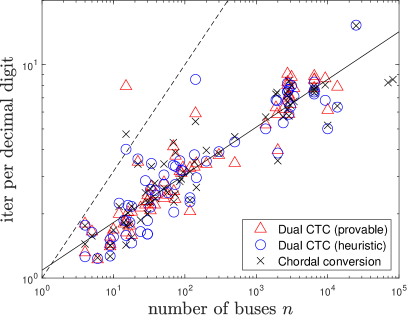
(b)

Figure 2: AC optimal power flow relaxation solved via chordal conversion ($\times$), heuristic Dual CTC ($\circ$), and provable Dual CTC ($\triangle$): (a) Time per iteration, with regression lines of $f_{\times}(n)=6.908n\times 10^{-5}$ with $R^{2}=0.90$, $f_{\circ}(n)=2.623n\times 10^{-4}$ with $R^{2}=0.83$, and $f_{\triangle}(n)=1.375n\times 10^{-3}$ with $R^{2}=0.80$; (b) Iterations per decimal digit of accuracy, with (solid) regression $g(n)=1.088n^{0.224}$ with $R^{2}=0.84$ and (dashed) bound $g(n)=\sqrt{n}$.

6.2 AC optimal power flow relaxation on real-world dataset

In the AC optimal power flow relaxation, the aggregate sparsity graph $G=(V,E)$ is a strict subgraph of the extended aggregate sparsity graph $\overline{G}=(V,\overline{E})$. We benchmark the following three conversion methods:

• CC: Chordal conversion as outlined in this paper in 1. We use the same implementation previously stated in 6.1. If $\overline{G}$ has small treewidth, then CC is guaranteed to use at most $O(m+n)$ time per-iteration via 3.1.

• Dual CTC (heuristic): The dualized variant of clique-tree conversion of Zhang and Lavaei [73]. We use the same implementation previously stated in 6.1. When $G\neq\overline{G}$, this variant reducs to an empirical heuristic.

• Dual CTC (provable): The extension of Gu and Song [30] to the dualized clique-tree conversion of Zhang and Lavaei [73]. If $\overline{G}$ has small treewidth, then this variant of Dual CTC is guaranteed to use at most $O(m+n)$ time per-iteration via [73, Theorem 1] and [30].

Here, the original (SDP) is posed over $X\in\mathbb{H}^{n}$, where $\mathbb{H}^{n}$ denotes the set of $n\times n$ complex Hermitian matrices. All three conversion methods are based on the complex Hermitian version of (CC), to avoid embedding the set of $n\times n$ complex Hermitian matrices into $\mathbb{S}^{2n}$. In all three cases, we use a dynamic programming algorithm [61, Algorithm 2] to recover a solution $U$ for the original SDP.

We perform one trial for each of 72 cases in the MATPOWER dataset. Here, recall that $\operatorname{tw}(G)=2\cdot\operatorname{tw}(\mathcal{G})$ and $\operatorname{tw}(\overline{G})=2\cdot\operatorname{tw}(\mathcal{G}^{2})$, where $\mathcal{G}$ is the graph of the underlying electric grid, and $\mathcal{G}^{2}$ is its square graph. We compute upper- and lower-bounds on the treewidths of $\mathcal{G}$ and $\mathcal{G}^{2}$ using the techniques outlined in [43]. Specifically, we use the minimum fill-in heuristic to compute a valid tree decomposition for each of $\mathcal{G}$ and $\mathcal{G}^{2}$, and the “MMD+” heuristic to compute lower-bounds on $\operatorname{tw}(\mathcal{G})$ and $\operatorname{tw}(\mathcal{G}^{2})$. The two conversion methods CC and Dual CTC (provable) require a tree decomposition for the extended graph $\overline{G}$ as an input to solve the SDP. The conversion method Dual CTC (heuristic) requires a tree decomposition for the graph $G$ instead. In each case, the tree decompositions are adapted from those for $\mathcal{G}$ and $\mathcal{G}^{2}$. 2 shows the treewidths of the graphs $\mathcal{G}$ and $\mathcal{G}^{2}$. The minimum fill-in heuristic is able to approximate the treewidth to a suboptimality ratio of 15. All 72 cases can be viewed as having small treewidth, although the treewidth for the largest three cases are still large enough to be an issue.

3 reports the accuracy and per-iteration of CC and Dual CTC for the 25 largest problems. Again, the “preprocessing” time includes the conversion process and MOSEK’s internal preparation time; the “postprocessing” time is the time taken to recover $U$ satisfying $\operatorname{proj}_{F}(UU^{T})=Y$ via [61, Algorithm 2]. For these smaller problems with $n$ less than $10^{5}$, the preprocessing times are all within a similar order of magnitude. For each method, the preprocessing time is about 0.5 to 3 times the cost of a single iteration. The postprocessing time costs as much as a single iteration of CC.

2 plots the per-iteration time, and the iterations-per-digit, all against the matrix order $n$. For this much more difficult problem, 2b does show a slightly increasing trend in the iterations-per-digit with respect to $n$. The regression line shows a fit of $g(n)=1.088n^{0.224}$, instead of the provable $O(\sqrt{n})$ figure shown as the dashed line. This same trend is much harder to see by looking at the raw iteration counts in 3, and the absolute maximum number of iterations remain no more than 120. 2a shows that CC is substantially faster than both variants of CTC. In fact, examining the details in 3, we see that CC is around a factor of 100 times faster than the provable variant of CTC, and around a factor of 2 faster than the heuristic version of CC.

7 Conclusions and future directions

Chordal conversion is a state-of-the-art algorithm for large-scale sparse SDP, but a definitive theoretical explanation for its superior performance was previously unknown. While it is folklore that the aggregate sparsity graph $G=(V,E)$, defined

$$V=\{1,2,\dots,n\},\quad E=\operatorname{spar}(C)\cup\operatorname{spar}(A_{1})\cup\cdots\cup\operatorname{spar}(A_{m}),$$

$$\text{where }\operatorname{spar}(C)\equiv\{(i,j):C[i,j]\neq 0\text{ for }i>j\},$$

needs to have small treewidth for the $O(m+n)$ time per-iteration figure, trivial counterexamples showed that a small treewidth in $G$ alone is not sufficient. In this paper, we fill this gap, by showing that a small treewidth in the extended aggregate sparsity graph $\overline{G}=(V,\overline{E})$, defined

$$V=\{1,2,\dots,n\},\quad\overline{E}=\operatorname{spar}(C)\cup\operatorname{clique}(A_{1})\cup\cdots\cup\operatorname{clique}(A_{m})$$

$$\text{where }\operatorname{clique}(A)=\{(i,j):A[i,k]\neq 0\text{ or }A[k,j]\neq 0\text{ for some }k\},$$

is indeed sufficient to guarantee $O(m+n)$ time per-iteration.

In the case that $G$ and $\overline{G}$ coincide, our analysis becomes exact; a small treewidth in $G=\overline{G}$ is both necessary and sufficient for chordal conversion to be fast. It remains future work to understand the cases where $G$ and $\overline{G}$ are very different. For example, if $C,A_{1},\dots,A_{m}$ are dense and diagonal, the graph $G$ is the empty graph with treewidth zero, the graph $\overline{G}$ is the complete graph on $n$ vertices with treewidth $n-1$, and the per-iteration cost is $\Omega(n^{3})$ time. This hints at the possibility that a small treewidth in $\overline{G}$ is both necessary and sufficient for $O(m+n)$ time per-iteration, but more work is establish this rigorously.

Acknowledgements

I am grateful to Martin S. Andersen for numerous insightful discussions, and for his early numerical experiments that motivated much of the subsequent theoretical analysis in this paper. The paper has also benefited significantly from discussions with Subhonmesh Bose, Salar Fattahi, Alejandro Dominguez–Garcia, Cedric Josz, and Sabrina Zielinski.

Financial support for this work was provided in part by the NSF CAREER Award ECCS-2047462 and in part by C3.ai Inc. and the Microsoft Corporation via the C3.ai Digital Transformation Institute.

Appendix A Running intersection property and zero-fill sparsity patterns

In this section, we prove a connection between zero-fill sparsity patterns, for which sequential Gaussian elimination results in no additionally fill-in, and a “sorted” extension of the running intersection property. We begin by formally defining zero-fill patterns.

Definition A.1 (ZF).

The sparsity pattern $F$ is said to be zero-fill if, for every $(i,k)\in F$ and $(j,k)\in F$ where $i>j>k$, there exists $(i,j)\in F$.

The columns of zero-fill sparsity patterns are the canonical example of sequence of subsets that satisfy the sorted version of the running intersection property.

Definition A.2 (RIP).

The sequence of subsets $J_{1},J_{2},\dots,J_{\ell}$ with $J_{j}\subset\mathbb{N}$ satisfies the sorted running intersection property if there exists a parent pointer $\operatorname{p}:\{1,2,\dots,\ell-1\}\to\{2,3,\dots,\ell\}$ such that the following holds for all $1\leq j<\ell$:

$$\operatorname{p}(j)>j,\quad J_{\operatorname{p}(j)}\supseteq J_{j}\cap(J_{j+1}\cup J_{j+2}\cup\cdots\cup J_{\ell}\},\quad\min\{J_{\operatorname{p}(j)}\}>\max\{J_{j}\backslash J_{\operatorname{p}(j)}\}.$$

Proposition A.3 (ZF$\implies$RIP).

Let $F$ be a zero-fill sparsity pattern of order $n$. Then, the sequence of subsets $J_{1},J_{2},\dots,J_{n}$ with $J_{j}=\operatorname{col}_{F}(j)\equiv\{j\}\cup\{i>j:(i,j)\in F\}$ satisfies the sorted running intersection property.

Proof.

Define $\operatorname{p}(j)=\min\{i>j:i\in J_{j}\}$ if $|J_{j}|>1$ and $p(j)=n$ if $|J_{j}|=1$. Clearly, $p(j)>j$ holds for all $1\leq j<n$. To prove $J_{\operatorname{p}(j)}\supseteq J_{j}\cap\bigcup_{w=j+1}^{\ell}J_{w}$, let $i\in J_{j}\cap J_{w}$ for some $w>j$. We prove that $i\in J_{\operatorname{p}(j)}$ via the following steps:

• We have $i>j$, because $i\in J_{w}$ implies that $i\geq w>j$.

• If $i=\operatorname{p}(j)$, then $i\in J_{\operatorname{p}(j)}$ by definition.

• If $i>p(j)$, then $(i,j)\in F$ and $(\operatorname{p}(j),j)\in F$ for $i>p(j)>j$ implies $(i,\operatorname{p}(j))\in F$, and hence $i\in J_{\operatorname{p}(j)}$.

Finally, we prove $\min\{J_{\operatorname{p}(j)}\}>\max\{J_{j}\backslash J_{\operatorname{p}(j)}\}$ by noting that $\max\{J_{j}\backslash J_{\operatorname{p}(j)}\}=j$ with our construction, and that $i=\min J_{\operatorname{p}(j)}$ must satisfy $i\in J_{\operatorname{p}(j)}$ and therefore $i\geq\operatorname{p}(j)>j$. ∎

In reverse, a sequence of subsets $J_{1},J_{2},\dots,J_{\ell}$ that satisfy the sorted running intersection property immediately give rise to a zero-fill sparsity pattern $F$. In this special case, it is possible to make an exact connection between the size of the subsets $|J_{k}|$ and the frontsize $\omega(F)$ of the sparsity pattern.

Proposition A.4 (RIP$\implies$ZF).

Let $J_{1},J_{2},\dots,J_{\ell}$ with $\bigcup_{j=1}^{\ell}J_{j}=\{1,2,\dots,n\}$ satisfy the sorted running intersection property. Then, the sparsity pattern $F=\bigcup_{j=1}^{\ell}\operatorname{clique}(J_{j})$ is zero-fill, and we have $\omega(F)=\max_{j}|J_{j}|$.

In the literature, variants of 4.7 are typically stated as the existence of a perfect elimination ordering $\Pi$ such that $\omega(\Pi F\Pi^{T})=\max_{k}|J_{k}|$. In this paper, we will further require the natural ordering $\Pi=I$ to explicitly be the perfect elimination ordering. This additional requirement necessitates the “sorted” part of the running intersection property.

Our proof of A.4 relies on the following result, which says that every column of $F$ is contain in a subset $J_{w}$.

Lemma A.5.

Let $J_{1},J_{2},\dots,J_{\ell}$ with $\bigcup_{j=1}^{\ell}J_{j}=\{1,2,\dots,n\}$ satisfy the ordered running intersection property. For every $j$-th column in $F=\bigcup_{j=1}^{\ell}\operatorname{clique}(J_{j})$, there exists some $J_{w}$ such that $\operatorname{col}_{F}(j)\subseteq J_{w}.$

Proof.

Let $V=\{1,2,\dots,n\}$. For arbitrary $j\in V$, denote $J_{w}$ as the last subset in the sequence $J_{1},J_{2},\dots,J_{\ell}$ for which $j\in J_{w}$. This choice must exist, because $V=\bigcup_{k=1}^{\ell}J_{k}$. For every arbitrary $i\in\operatorname{col}(j)$, we will prove that $i\in J_{w}$ also holds:

• There exists $u\leq w$ for which $i,j\in J_{u}$. Indeed, $(i,j)\in E$ and $E=\bigcup_{k=1}^{\ell}\operatorname{clique}(J_{k})$ imply the existence of $J_{u}$ for which $i,j\in J_{u}$. Given that $j\in J_{u}$ and $w=\max\{k:j\in J_{k}\}$ by definition, it follows that $u\leq w$.

• If $u=w$, then $i\in J_{w}$ holds because $i,j\in J_{u}$. Otherwise, if $u<w$, we use the sorted running intersection property to assert the following

  $$u<w,\qquad i,j\in J_{u}\quad\implies\quad i,j\in J_{\operatorname{p}(u)}.$$ (10)

  The fact that $j\in J_{\operatorname{p}(u)}$ follows directly the running intersection property $j\in J_{u}\cap J_{w}\subseteq J_{\operatorname{p}(u)}$ for $w>u$. By contradiction, suppose that $i\notin J_{\operatorname{p}(u)}$. Then, given that $i\in J_{u}$, it follows from the sorted property that $k\geq\min\{J_{\operatorname{p}(u)}\}>\max\{J_{u}\backslash J_{\operatorname{p}(u)}\}\geq i,$ which contradicts our initial hypothesis that $i>k$.

• Inductively reapplying (10), as in $i,j\in J_{\operatorname{p}(\operatorname{p}(u))}$ and $i,j\in J_{\operatorname{p}(\operatorname{p}(\operatorname{p}(u)))}$, we arrive at some $v$ such that $i,j\in J_{\operatorname{p}(v)}$ and $p(v)=w$. The induction must terminate with $p(v)\geq w$ because each $\operatorname{p}(u)>u$ by construction. It is impossible for $\operatorname{p}(v)>w$ to occur, because $j\in J_{\operatorname{p}(v)}$ and $w=\max\{k:j\in J_{k}\}$ by definition. We conclude that $i\in J_{w}$, as desired.

∎

The equivalence between the sorted running intersection property and zero-fill sparsity pattern then follow as a short corrollary of the above.

Proof of A.4.

To prove that $F$ is zero-fill, we observe, for arbitrary $(i,k)\in F$ and $(j,k)\in F$ with $i>j>k$ that $i,j\in\operatorname{col}_{F}(k)$. Therefore, it follows from A.5 that there exists $J_{w}$ such that $i,j,k\in J_{w}$. We conclude that $(i,j)\in F,$ because $F=\bigcup_{j=1}^{\ell}\operatorname{clique}(J_{j})$ and $i,j\in J_{w}$ for some $1\leq w\leq\ell$.

To prove that $\omega(F)=\max_{j}|J_{j}|$, we choose $k=\arg\max_{j}|\operatorname{col}_{F}(j)|$. It follows from Lemma A.5 that there exists $J_{w}$ such that $\operatorname{col}_{F}(k)\subseteq J_{w}$, and therefore $\omega(E)=|\operatorname{col}_{F}(k)|\leq|J_{w}|$. Finally, given that $\operatorname{clique}(J_{w})\subseteq F$ it follows that $(i,j)\in F$ holds for all $i\in J_{w}$ where $j=\min J_{w}$. Therefore, we conclude that $J_{w}\subseteq\operatorname{col}_{F}(j)$, and therefore $|J_{w}|\leq|\operatorname{col}_{F}(j)|\leq|\operatorname{col}_{F}(k)|=\omega(F)$. ∎

Appendix B Complexity of general-purpose interior-point methods

A general-purpose interior-point method takes $(\mathbf{A},\mathbf{b},\mathbf{c},\mathcal{K})$ as input, and computes a primal-dual pair $(x,y)$ for the corresponding instance of the standard-form linear conic program primal-dual pair:

$$\min_{x\in\mathbb{R}^{N}}\{\mathbf{c}^{T}x:\mathbf{A}x=b,x\in\mathcal{K}\}=\max_{y\in\mathbb{R}^{M}}\{\mathbf{b}^{T}y:\mathbf{c}-\mathbf{A}^{T}y\in\mathcal{K}\}.$$ (11)

In order for this to yield a polynomial time guarantee, the problem must satisfy two regularity conditions.

Definition B.1.

We say that the problem data $\mathbf{A}\in\mathbb{R}^{M\times N},$ $\mathbf{b}\in\mathbb{R}^{M},$ $\mathbf{c}\in\mathbb{R}^{N},$ and problem cone $\mathcal{K}$ describe an SDP in $(n,\omega)$-standard form if:

1. (Dimensions) The cone $\mathcal{K}=\operatorname{svec}(\mathbb{S}_{+}^{\omega_{1}})\times\cdots\times\operatorname{svec}(\mathbb{S}_{+}^{\omega_{\ell}})$ is the Cartesian product of semidefinite cones whose orders $\omega_{1},\omega_{2},\dots,\omega_{\ell}$ satisfy

   $$\omega=\max_{i}\omega_{i},\quad n=\sum_{i=1}^{\ell}\omega_{i},\quad N=\frac{1}{2}\sum_{i=1}^{\ell}\omega_{i}(\omega_{i}+1).$$

2. (Linear independence) $\mathbf{A}^{T}y=0$ holds if and only if $y=0$.

3. (Strong duality) There exist a choice of $x^{\star},y^{\star},s^{\star}$ that satisfy

   $$\mathbf{A}^{T}x^{\star}=\mathbf{b},\quad\mathbf{A}^{T}y^{\star}+s^{\star}=\mathbf{c},\quad(x^{\star})^{T}s^{\star}=0,\quad x^{\star},s^{\star}\in\mathcal{K}.$$

Proposition B.2.

Let $(\mathbf{A},\mathbf{b},\mathbf{c},\mathcal{K})$ describe an SDP in $(n,\omega)$-standard form, and let $\mathrm{opt}$ denote its optimal value. Let $\mathsf{T}$ and $\mathsf{M}$ denote the time and memory needed, given data $\mathbf{A}\in\mathbb{R}^{M\times N}$, $g\in\mathbb{R}^{M}$, and a choice of $w\in\operatorname{Int}(\mathcal{K})$, to form and solve $\mathbf{A}\mathbf{D}\mathbf{A}^{T}\Delta y=g$ for $\Delta y\in\mathbb{R}^{m}$, where $\mathbf{D}^{-1}=\nabla^{2}f(w)$ and $f=-\log\det(w)$. Then, a general-purpose interior-point method computes $(x,y)$ that satisfy the following in $O(\sqrt{n}\log(1/\epsilon))$ iterations

$$\mathbf{c}^{T}x\leq\mathrm{opt}+n\cdot\epsilon,\quad\|\mathbf{A}x-\mathbf{b}\|\leq\epsilon,\quad x\in\mathcal{K},$$

$$\mathbf{b}^{T}y\geq\mathrm{opt}-n\cdot\epsilon,\quad\mathbf{c}-\mathbf{A}^{T}y+\epsilon\mathbf{1}_{\mathcal{K}}\in\mathcal{K},$$

with per-iteration costs of $O(\omega^{2}n+\operatorname{nnz}(\mathbf{A})+\mathsf{T})$ time and $O(\omega n+\operatorname{nnz}(\mathbf{A})+\mathsf{M})$ memory.

We prove B.2 by solving (11) via its extended homogeneous self-dual embedding

$$\min_{x,y,s,\kappa,\tau,\theta}\quad (n+1)\theta$$ (12a)

s.t. $$\begin{bmatrix}0&+\mathbf{A}^{T}&-\mathbf{c}&-r_{d}\\ -\mathbf{A}&0&+\mathbf{b}&-r_{p}\\ +\mathbf{c}^{T}&-\mathbf{b}^{T}&0&-r_{c}\\ r_{d}^{T}&r_{p}^{T}&r_{c}&0\end{bmatrix}\begin{bmatrix}x\\ y\\ \tau\\ \theta\end{bmatrix}+\begin{bmatrix}s\\ 0\\ \kappa\\ 0\end{bmatrix} =\begin{bmatrix}0\\ 0\\ 0\\ n+1\end{bmatrix}$$ (12b)

$$x,s\in\mathcal{K},\quad\kappa,\tau \geq 0,$$ (12c)

where the residual vectors are defined

$$r_{d}=\mathbf{1}_{\mathcal{K}}-\mathbf{c},\quad r_{p}=-\mathbf{A}\mathbf{1}_{\mathcal{K}}+\mathbf{b},\quad r_{c}=1+\mathbf{c}^{T}\mathbf{1}_{\mathcal{K}}.$$ (12d)

The main motivation for the embedding is to be able to start an interior-point method at an initial point that is both strictly feasible and lies perfectly centered on the central path:

$$\theta^{(0)}=\tau^{(0)}=\kappa^{(0)}=1,\quad y^{(0)}=0,\quad x^{(0)}=s^{(0)}=\mathbf{1}_{\mathcal{K}}.$$ (13)

In this paper, we use the short-step method of Nesterov and Todd [48, Algorithm 6.1] (and also Sturm and S. Zhang [60, Section 5.1]), noting that SeDuMi reduces to it in the worst case; see [58] and [59]. Beginning at the strictly feasible, perfectly centered point for $\mu=1$ stated in (13), we take the following steps

$$\mu^{+} =\left(1-\frac{1}{15\sqrt{n+1}}\right)\cdot\frac{x^{T}s+\tau\kappa}{n+1},$$ (14a)

$$(x^{+},y^{+},s^{+},\tau^{+},\theta^{+},\kappa^{+}) =(x,y,s,\tau,\theta,\kappa)+(\Delta x,\Delta y,\Delta s,\Delta\tau,\Delta\theta,\Delta\kappa).$$

along the search direction defined by the linear system [63, Eqn. 9]

$$\begin{bmatrix}0&+\mathbf{A}^{T}&-\mathbf{c}&-r_{p}\\ -\mathbf{A}&0&+\mathbf{b}&-r_{d}\\ +\mathbf{c}^{T}&-\mathbf{b}^{T}&0&-r_{c}\\ +r_{p}^{T}&+r_{d}^{T}&+r_{c}&0\end{bmatrix}\begin{bmatrix}\Delta x\\ \Delta y\\ \Delta\tau\\ \Delta\theta\end{bmatrix}+\begin{bmatrix}\Delta s\\ 0\\ \Delta\kappa\\ 0\end{bmatrix} =0,$$ (15a)

$$s+\Delta s+\nabla^{2}f(w)\Delta x+\mu^{+}\nabla f(x) =0,$$ (15b)

$$\kappa+\Delta\kappa+(\kappa/\tau)\Delta\tau-\mu^{+}\tau^{-1} =0.$$ (15c)

where $f(w)=-\log\det w$ is the usual self-concordant barrier function. The scaling point $w\in\operatorname{Int}(\mathcal{K})$ is the unique point that satisfies $\nabla^{2}f(w)x=s$. The following iteration bound is an immediate consequence of [48, Theorem 6.4]; see also [60, Theorem 5.1].

Lemma B.3 (Short-Step Method).

The sequence in (14) arrives at an iterate $(x,y,s,\tau,\theta,\kappa)$ satisfying

$$\frac{x^{T}s+\tau\kappa}{n+1}\leq\epsilon,\qquad\tau\kappa\geq\gamma\epsilon$$ (16)

with $\gamma=\frac{9}{10}$ in at most $O(\sqrt{n}\log(1/\epsilon))$ iterations.

Finally, the following result assures us that the interior-point method will converge to a point with $\tau>0$ and $\theta\to 0$ and $\kappa\to 0$, from which we can recover a solution to the original problem. The result is adapted from [73, Lemma 12], which was in turn adapted from [17, Lemma 5.7.2] and [67, Theorem 22.7].

Lemma B.4 ($\epsilon$-accurate and $\epsilon$-feasible).

Let there exist $(x^{\star},y^{\star})$ such that $\mathbf{A}x^{\star}=\mathbf{b}$ with $x^{\star}\in\mathcal{K}$ and $\mathbf{c}-\mathbf{A}^{T}y^{\star}\in\mathcal{K}$ that satisfies strong duality $\mathbf{b}^{T}y^{\star}=\mathbf{c}^{T}x^{\star}$. Then, a point $(x,y,s,\tau,\theta,\kappa)$ that is feasible for (12) and satisfies the optimality condition (16) also satisfies the following

$$\|\mathbf{A}(x/\tau)-\mathbf{b}\| \leq\frac{\rho\|r_{p}\|}{\gamma}\cdot\epsilon, \|\mathbf{A}^{T}(y/\tau)+(s/\tau)-\mathbf{c}\| \leq\frac{\rho\|r_{d}\|}{\gamma}\cdot\epsilon, \frac{(x/\tau)^{T}(s/\tau)}{n+1}\leq\frac{\rho^{2}}{\gamma^{2}}\cdot\epsilon$$

where $\rho=1+\mathbf{1}_{\mathcal{K}}^{T}(x^{\star}+s^{\star})$.

Proof.

Let $s^{\star}=\mathbf{c}-\mathbf{A}^{T}y^{\star}$. First, we observe that $(\hat{x},\hat{y},\hat{s},\hat{\tau},\hat{\theta},\hat{\kappa})=(\hat{\tau}x^{\star},\hat{\tau}y^{\star},\hat{\tau}s^{\star},\hat{\tau},0,0)$ with

$$\hat{\tau}=\frac{n+1}{r_{d}^{T}x^{\star}+r_{p}^{T}y^{\star}+r_{c}}=\frac{n+1}{\mathbf{1}_{\mathcal{K}}^{T}(x^{\star}+s^{\star})+1}=\frac{n+1}{\rho},$$

is a solution to (12). Next, note that if $(x,y,s,\tau,\theta,\kappa)$ is feasible for (12), meaning that it satisfies (12b) and (12c), then it follows from the skew-symmetry of (12b) that $\theta=\frac{x^{T}s+\tau\kappa}{n+1}$ and that $(x-\hat{x})^{T}(s-\hat{s})+(\tau-\hat{\tau})(\kappa-\hat{\kappa})=0.$ Rearranging yields $(n+1)\theta=x^{T}s+\tau\kappa=\hat{x}^{T}s+x^{T}\hat{s}+\tau\hat{\kappa}+\hat{\tau}\kappa$ and hence

$$(n+1)\theta\geq\kappa\hat{\tau},\quad\tau\kappa\geq\gamma\theta\qquad\implies\qquad\tau\geq\frac{\gamma\theta}{\kappa}\geq\frac{\gamma\theta}{(n+1)\theta/\hat{\tau}}=\frac{\gamma}{n+1}\hat{\tau}=\frac{\gamma}{\rho}.$$

Therefore, every $(x,y,s,\tau,\theta,\kappa)$ that is feasible for (12) must have $\tau$ that is lower-bounded $\tau\geq\gamma/\rho$. Finally, we divide (12b) through by $\tau$ and find that

$$\|\mathbf{A}(x/\tau)-\mathbf{b}\| =\frac{\|r_{p}\|\theta}{\tau}, \|\mathbf{A}^{T}(y/\tau)+(s/\tau)-\mathbf{c}\| =\frac{\|r_{d}\|\theta}{\tau}, \frac{(x/\tau)^{T}(s/\tau)}{n+1}=\frac{\theta}{\tau^{2}}.$$

Substituting the lower-bound $1/\tau\leq\rho/\gamma$ yields our desired result. ∎

Proof of B.2.

Recall that $(\mathbf{A},\mathbf{b},\mathbf{c},\mathcal{K})$ describe an SDP in $(n,\omega)$-standard form, and hence there exist $(x^{\star},y^{\star})$ such that $\mathbf{A}x^{\star}=\mathbf{b}$ with $x^{\star}\in\mathcal{K}$ and $\mathbf{c}-\mathbf{A}^{T}y^{\star}\in\mathcal{K}$ that satisfies strong duality $\mathbf{b}^{T}y^{\star}=\mathbf{c}^{T}x^{\star}$. Combining B.4 and B.3 shows that iterations in (14) converges to the desired $\epsilon$-accurate, $\epsilon$-feasible iterate after $O(\sqrt{n}\log(1/\epsilon))$ iterations. The cost of each iteration is essentially equal to the cost of computing the search direction in (15). We account for this cost via the following two steps:

1. (Scaling point) We partition $x=[\operatorname{svec}(X_{j})]_{j=1}^{\ell}$ and $s=[\operatorname{svec}(S_{j})]_{j=1}^{\ell}$. Then, the scaling point $w=[\operatorname{svec}(W_{j})]_{j=1}^{\ell}$ is given in closed-form [58, Section 5]

   $$W_{j}=S_{j}^{1/2}(S_{j}^{1/2}X_{j}S_{j}^{1/2})^{-1/2}S_{j}^{1/2}.$$

   Noting that each $W_{j}$ is at most $\omega\times\omega$, the cost of forming $w$ is at most of order

   $$\sum_{j=1}^{\ell}\omega_{j}^{3}\leq\omega^{2}\sum_{j=1}^{\ell}\omega_{j}=\omega^{2}n\text{ time},\quad\sum_{j=1}^{\ell}\omega_{j}^{2}\leq\omega\sum_{j=1}^{\ell}\omega_{j}=\omega n\text{ memory.}$$

   By this same calculation, it follows that the Hessian matrix-vector products $\nabla^{2}f(w)x=[\operatorname{svec}(W_{j}^{-1}X_{j}W_{j}^{-1})]_{j=1}^{\ell}$ and $\nabla^{2}f(w)^{-1}x=[\operatorname{svec}(W_{j}X_{j}W_{j})]_{j=1}^{\ell}$ also cost $O(\omega^{2}n)$ time and $O(\omega n)$ memory.

2. (Search direction) Using elementary but tedious linear algebra, we can show that if

   $$(\mathbf{A}\mathbf{D}\mathbf{A}^{T})\begin{bmatrix}v_{1}&v_{2}&v_{3}\end{bmatrix}=\begin{bmatrix}0&-\mathbf{b}&r_{p}\end{bmatrix}-\mathbf{A}\mathbf{D}\begin{bmatrix}d&\mathbf{c}&r_{d}\end{bmatrix}$$ (17a)

   where $$\mathbf{D}=[\nabla^{2}f(w)]^{-1} d=-s-\mu^{+}\nabla f(x)$$ and , and

   $$\begin{bmatrix}u_{1}&u_{2}&u_{3}\end{bmatrix}=\mathbf{D}(\begin{bmatrix}d&c&r_{d}\end{bmatrix}+\mathbf{A}^{T}\begin{bmatrix}v_{1}&v_{2}&v_{3}\end{bmatrix}),$$ (17b)

   then

   $$\left(\begin{bmatrix}-\mathbf{D}_{0}^{-1}&-r_{c}\\ r_{c}&0\end{bmatrix}-\begin{bmatrix}\mathbf{c}&r_{d}\\ -\mathbf{b}&r_{p}\end{bmatrix}^{T}\begin{bmatrix}u_{2}&u_{3}\\ v_{2}&v_{3}\end{bmatrix}\right)\begin{bmatrix}\Delta\tau\\ \Delta\theta\end{bmatrix} =\begin{bmatrix}-d_{0}\\ 0\end{bmatrix}-\begin{bmatrix}\mathbf{c}&r_{d}\\ -\mathbf{b}&r_{p}\end{bmatrix}^{T}\begin{bmatrix}u_{1}\\ v_{1}\end{bmatrix},$$ (17c)

   $$\begin{bmatrix}\Delta x\\ \Delta y\end{bmatrix} =\begin{bmatrix}u_{1}\\ v_{1}\end{bmatrix}-\begin{bmatrix}u_{1}&u_{2}\\ v_{1}&v_{2}\end{bmatrix}\begin{bmatrix}\Delta\tau\\ \Delta\theta\end{bmatrix},$$ (17d)

   $$\Delta s =d-\mathbf{D}^{-1}\Delta x,$$ (17e)

   $$\Delta\kappa =d_{0}-\mathbf{D}_{0}^{-1}\Delta\tau,$$ (17f)

   where $\mathbf{D}_{0}=\tau/\kappa$ and $d_{0}=-\kappa+\mu^{+}\tau^{-1}$. Therefore, we conclude that the cost of computing the search direction in (15) is equal to the cost of solving $O(1)$ instances of the normal equation $\mathbf{A}\mathbf{D}\mathbf{A}^{T}\Delta y=g$, plus $O(1)$ matrix-vector products with $\mathbf{A},\mathbf{A}^{T},\mathbf{D},\mathbf{D}^{-1}$, for a total cost of $O(\mathsf{T}+\operatorname{nnz}(\mathbf{A})+\omega^{2}n)$ time and $O(\mathsf{M}+\operatorname{nnz}(\mathbf{A})+\omega n)$ memory respectively. Note that $\mathbf{A}\mathbf{D}\mathbf{A}^{T}\succ 0$ because $\mathbf{A}\mathbf{A}^{T}\succ 0$ by the linear independence assumption, and $\mathbf{D}^{-1}=\nabla^{2}f(w)\succ 0$ for all $w\in\operatorname{Int}(\mathcal{K})$.

∎

References

- Amestoy et al. [2004] Patrick R Amestoy, Timothy A Davis, and Iain S Duff. Algorithm 837: AMD, an approximate minimum degree ordering algorithm. ACM Transactions on Mathematical Software (TOMS), 30(3):381–388, 2004.
- Andersen and Andersen [2000] Erling D Andersen and Knud D Andersen. The MOSEK interior point optimizer for linear programming: an implementation of the homogeneous algorithm. In High Performance Optimization, pages 197–232. Springer, 2000.
- Andersen et al. [2003] Erling D Andersen, Cornelis Roos, and Tamas Terlaky. On implementing a primal-dual interior-point method for conic quadratic optimization. Mathematical Programming, 95:249–277, 2003.
- Bai and Wei [2009] X Bai and H Wei. Semi-definite programming-based method for security-constrained unit commitment with operational and optimal power flow constraints. IET Generation, Transmission & Distribution, 3(2):182–197, 2009.
- Bai et al. [2008] Xiaoqing Bai, Hua Wei, Katsuki Fujisawa, and Yong Wang. Semidefinite programming for optimal power flow problems. International Journal of Electrical Power & Energy Systems, 30(6-7):383–392, 2008.
- Birchfield et al. [2016] Adam B Birchfield, Ti Xu, Kathleen M Gegner, Komal S Shetye, and Thomas J Overbye. Grid structural characteristics as validation criteria for synthetic networks. IEEE Transactions on power systems, 32(4):3258–3265, 2016.
- Bodlaender [1996] Hans L Bodlaender. A linear-time algorithm for finding tree-decompositions of small treewidth. SIAM Journal on computing, 25(6):1305–1317, 1996.
- Bodlaender et al. [2016] Hans L Bodlaender, Pal Gronas Drange, Markus S Dregi, Fedor V Fomin, Daniel Lokshtanov, and Michal Pilipczuk. A c^kn 5-approximation algorithm for treewidth. SIAM Journal on Computing, 45(2):317–378, 2016.
- Borchers [1999] Brian Borchers. Sdplib 1.2, a library of semidefinite programming test problems. Optimization Methods and Software, 11(1-4):683–690, 1999.
- Boumal [2015] Nicolas Boumal. A riemannian low-rank method for optimization over semidefinite matrices with block-diagonal constraints. arXiv preprint arXiv:1506.00575, 2015.
- Boumal et al. [2016] Nicolas Boumal, Vladislav Voroninski, and Afonso S Bandeira. The non-convex burer-monteiro approach works on smooth semidefinite programs. arXiv preprint arXiv:1606.04970, 2016.
- Boumal et al. [2020] Nicolas Boumal, Vladislav Voroninski, and Afonso S Bandeira. Deterministic guarantees for burer-monteiro factorizations of smooth semidefinite programs. Communications on Pure and Applied Mathematics, 73(3):581–608, 2020.
- Burer and Monteiro [2003] Samuel Burer and Renato DC Monteiro. A nonlinear programming algorithm for solving semidefinite programs via low-rank factorization. Math. Program., 95(2):329–357, 2003.
- Cai et al. [2010] Jian-Feng Cai, Emmanuel J Candès, and Zuowei Shen. A singular value thresholding algorithm for matrix completion. SIAM Journal on optimization, 20(4):1956–1982, 2010.
- Chiu and Zhang [2023] Hong-Ming Chiu and Richard Y Zhang. Tight certification of adversarially trained neural networks via nonconvex low-rank semidefinite relaxations. In International Conference on Machine Learning. PMLR, 2023.
- Dancis [1992] Jerome Dancis. Positive semidefinite completions of partial hermitian matrices. Linear algebra and its applications, 175:97–114, 1992.
- de Klerk et al. [2000] Etienne de Klerk, Tamás Terlaky, and Kees Roos. Self-dual embeddings. In Handbook of Semidefinite Programming, pages 111–138. Springer, 2000.
- Dong et al. [2021] Sally Dong, Yin Tat Lee, and Guanghao Ye. A nearly-linear time algorithm for linear programs with small treewidth: a multiscale representation of robust central path. In Proceedings of the 53rd Annual ACM SIGACT Symposium on Theory of Computing, pages 1784–1797, 2021.
- Eltved et al. [2019] Anders Eltved, Joachim Dahl, and Martin S. Andersen. On the robustness and scalability of semidefinite relaxation for optimal power flow problems. Optimization and Engineering, Mar 2019. ISSN 1573-2924. doi: 10.1007/s11081-019-09427-4. URL https://doi.org/10.1007/s11081-019-09427-4.
- Fomin et al. [2018] Fedor V Fomin, Daniel Lokshtanov, Saket Saurabh, Michał Pilipczuk, and Marcin Wrochna. Fully polynomial-time parameterized computations for graphs and matrices of low treewidth. ACM Transactions on Algorithms (TALG), 14(3):1–45, 2018.
- Frieze and Jerrum [1997] Alan Frieze and Mark Jerrum. Improved approximation algorithms for MAX k-CUT and MAX BISECTION. Algorithmica, 18(1):67–81, 1997.
- Fujisawa et al. [2009] Katsuki Fujisawa, Sunyoung Kim, Masakazu Kojima, Y Okamoto, and Makoto Yamashita. User’s manual for SparseCoLO: Conversion methods for sparse conic-form linear optimization problems. Report B-453, Dept. of Math. and Comp. Sci. Japan, Tech. Rep, pages 152–8552, 2009.
- Fukuda et al. [2001] Mituhiro Fukuda, Masakazu Kojima, Kazuo Murota, and Kazuhide Nakata. Exploiting sparsity in semidefinite programming via matrix completion I: General framework. SIAM J. Optim., 11(3):647–674, 2001.
- George and Liu [1981] Alan George and Joseph W Liu. Computer solution of large sparse positive definite. Prentice Hall Professional Technical Reference, 1981.
- Goemans and Williamson [1995] Michel X Goemans and David P Williamson. Improved approximation algorithms for maximum cut and satisfiability problems using semidefinite programming. J. ACM, 42(6):1115–1145, 1995.
- Griewank and Toint [1982a] Andreas Griewank and Ph L Toint. Partitioned variable metric updates for large structured optimization problems. Numerische Mathematik, 39(1):119–137, 1982a.
- Griewank and Toint [1984] Andreas Griewank and Ph L Toint. On the existence of convex decompositions of partially separable functions. Mathematical Programming, 28(1):25–49, 1984.
- Griewank and Toint [1982b] Andreas Griewank and Philippe Toint. On the unconstrained optimization of partially separable functions. In Nonlinear Optimization 1981, pages 301–312. Academic press, 1982b.
- Grone et al. [1984] Robert Grone, Charles R Johnson, Eduardo M Sá, and Henry Wolkowicz. Positive definite completions of partial hermitian matrices. Linear Algebra Appl., 58:109–124, 1984.
- Gu and Song [2022] Yuzhou Gu and Zhao Song. A faster small treewidth sdp solver. arXiv preprint arXiv:2211.06033, 2022.
- Jabr [2006] Rabih A Jabr. Radial distribution load flow using conic programming. IEEE transactions on power systems, 21(3):1458–1459, 2006.
- Jabr [2012] Rabih A Jabr. Exploiting sparsity in SDP relaxations of the OPF problem. IEEE Transactions on Power Systems, 27(2):1138–1139, 2012.
- Jaggi [2013] Martin Jaggi. Revisiting frank-wolfe: Projection-free sparse convex optimization. In International conference on machine learning, pages 427–435. PMLR, 2013.
- Josz et al. [2016] Cédric Josz, Stéphane Fliscounakis, Jean Maeght, and Patrick Panciatici. Ac power flow data in matpower and qcqp format: itesla, rte snapshots, and pegase. arXiv preprint arXiv:1603.01533, 2016.
- Kim et al. [2009] Sunyoung Kim, Masakazu Kojima, and Hayato Waki. Exploiting sparsity in sdp relaxation for sensor network localization. SIAM Journal on Optimization, 20(1):192–215, 2009.
- Kim et al. [2011] Sunyoung Kim, Masakazu Kojima, Martin Mevissen, and Makoto Yamashita. Exploiting sparsity in linear and nonlinear matrix inequalities via positive semidefinite matrix completion. Math. Program., 129(1):33–68, 2011.
- Kobayashi et al. [2008] Kazuhiro Kobayashi, Sunyoung Kim, and Masakazu Kojima. Correlative sparsity in primal-dual interior-point methods for lp, sdp, and socp. Appl. Math. Optim., 58(1):69–88, 2008.
- Laue [2012] Sören Laue. A hybrid algorithm for convex semidefinite optimization. In Proceedings of the 29th International Coference on International Conference on Machine Learning, pages 1083–1090, 2012.
- Lavaei and Low [2012] Javad Lavaei and Steven H Low. Zero duality gap in optimal power flow problem. IEEE Transactions on Power Systems, 27(1):92, 2012.
- Liu [1990] Joseph WH Liu. The role of elimination trees in sparse factorization. SIAM J. Matrix Anal. Appl., 11(1):134–172, 1990.
- Lovász [1979] László Lovász. On the shannon capacity of a graph. IEEE Trans. Inf. Theory, 25(1):1–7, 1979.
- Madani et al. [2016] Ramtin Madani, Morteza Ashraphijuo, and Javad Lavaei. Promises of conic relaxation for contingency-constrained optimal power flow problem. IEEE Trans. Power Syst., 31(2):1297–1307, 2016.
- Maniu et al. [2019] Silviu Maniu, Pierre Senellart, and Suraj Jog. An experimental study of the treewidth of real-world graph data. In 22nd International Conference on Database Theory (ICDT 2019). Schloss Dagstuhl-Leibniz-Zentrum fuer Informatik, 2019.
- Molzahn and Hiskens [2014] Daniel K Molzahn and Ian A Hiskens. Sparsity-exploiting moment-based relaxations of the optimal power flow problem. IEEE Transactions on Power Systems, 30(6):3168–3180, 2014.
- Molzahn et al. [2013] Daniel K Molzahn, Jesse T Holzer, Bernard C Lesieutre, and Christopher L DeMarco. Implementation of a large-scale optimal power flow solver based on semidefinite programming. IEEE Transactions on Power Systems, 28(4):3987–3998, 2013.
- MOSEK ApS [2019] MOSEK ApS. The MOSEK optimization toolbox for MATLAB manual. Version 9.0., 2019. URL {http://docs.mosek.com/9.0/toolbox/index.html}.
- Nesterov [2005] Yu Nesterov. Smooth minimization of non-smooth functions. Mathematical programming, 103:127–152, 2005.
- Nesterov and Todd [1998] Yu E Nesterov and Michael J Todd. Primal-dual interior-point methods for self-scaled cones. SIAM Journal on optimization, 8(2):324–364, 1998.
- Nesterov [2007] Yurii Nesterov. Smoothing technique and its applications in semidefinite optimization. Mathematical Programming, 110(2):245–259, 2007.
- O’Carroll et al. [2022] Liam O’Carroll, Vaidehi Srinivas, and Aravindan Vijayaraghavan. The burer-monteiro sdp method can fail even above the barvinok-pataki bound. Advances in Neural Information Processing Systems, 35, 2022.
- Pataki and Schmieta [2002] Gabor Pataki and Stefan Schmieta. The dimacs library of semidefinite-quadratic-linear programs, 2002. URL http://archive.dimacs.rutgers.edu/Challenges/Seventh/Instances/.
- Rose [1970] Donald J Rose. Triangulated graphs and the elimination process. Journal of Mathematical Analysis and Applications, 32(3):597–609, 1970.
- Rose [1972] Donald J Rose. A graph-theoretic study of the numerical solution of sparse positive definite systems of linear equations, pages 183–217. Elsevier, 1972.
- Rose et al. [1976] Donald J. Rose, R. Endre Tarjan, and George S. Lueker. Algorithmic aspects of vertex elimination on graphs. SIAM Journal on Computing, 5(2):266–283, 1976. doi: 10.1137/0205021.
- Rosen et al. [2019] David M Rosen, Luca Carlone, Afonso S Bandeira, and John J Leonard. Se-sync: A certifiably correct algorithm for synchronization over the special euclidean group. The International Journal of Robotics Research, 38(2-3):95–125, 2019.
- Rosen et al. [2020] David M Rosen, Luca Carlone, Afonso S Bandeira, and John J Leonard. A certifiably correct algorithm for synchronization over the special euclidean group. In Algorithmic Foundations of Robotics XII, pages 64–79. Springer, 2020.
- Sturm [1999] Jos F Sturm. Using sedumi 1.02, a matlab toolbox for optimization over symmetric cones. Optim. Method. Softw., 11(1-4):625–653, 1999.
- Sturm [2002] Jos F Sturm. Implementation of interior point methods for mixed semidefinite and second order cone optimization problems. Optimization methods and software, 17(6):1105–1154, 2002.
- Sturm and Zhang [1997] Jos F Sturm and Shuzhong Zhang. On a wide region of centers and primal-dual interior point algorithms for linear programming. Mathematics of Operations Research, 22(2):408–431, 1997.
- Sturm and Zhang [1999] Jos F Sturm and Shuzhong Zhang. Symmetric primal-dual path-following algorithms for semidefinite programming. Applied Numerical Mathematics, 29(3):301–315, 1999.
- Sun [2015] Yifan Sun. Decomposition methods for semidefinite optimization. PhD thesis, UCLA, 2015. URL https://escholarship.org/uc/item/1cv6981p.
- Sun et al. [2014] Yifan Sun, Martin S Andersen, and Lieven Vandenberghe. Decomposition in conic optimization with partially separable structure. SIAM J. Optim., 24(2):873–897, 2014.
- Todd et al. [1998] Michael J Todd, Kim-Chuan Toh, and Reha H Tütüncü. On the nesterov–todd direction in semidefinite programming. SIAM Journal on Optimization, 8(3):769–796, 1998.
- Toh et al. [1999] Kim-Chuan Toh, Michael J Todd, and Reha H Tütüncü. Sdpt3–a matlab software package for semidefinite programming, version 1.3. Optimization methods and software, 11(1-4):545–581, 1999.
- Tütüncü et al. [2003] Reha H Tütüncü, Kim-Chuan Toh, and Michael J Todd. Solving semidefinite-quadratic-linear programs using sdpt3. Mathematical programming, 95:189–217, 2003.
- Vandenberghe et al. [2015] Lieven Vandenberghe, Martin S Andersen, et al. Chordal graphs and semidefinite optimization. Foundations and Trends in Optimization, 1(4):241–433, 2015.
- Vanderbei [2015] Robert J Vanderbei. Linear programming: Foundations and Extensions. Springer, 2015.
- Waki et al. [2006] Hayato Waki, Sunyoung Kim, Masakazu Kojima, and Masakazu Muramatsu. Sums of squares and semidefinite program relaxations for polynomial optimization problems with structured sparsity. SIAM Journal on Optimization, 17(1):218–242, 2006.
- Waki et al. [2008] Hayato Waki, Sunyoung Kim, Masakazu Kojima, Masakazu Muramatsu, and Hiroshi Sugimoto. Algorithm 883: Sparsepop—a sparse semidefinite programming relaxation of polynomial optimization problems. ACM Transactions on Mathematical Software (TOMS), 35(2):1–13, 2008.
- Waldspurger and Waters [2020] Irene Waldspurger and Alden Waters. Rank optimality for the burer–monteiro factorization. SIAM journal on Optimization, 30(3):2577–2602, 2020.
- Wen et al. [2010] Zaiwen Wen, Donald Goldfarb, and Wotao Yin. Alternating direction augmented lagrangian methods for semidefinite programming. Mathematical Programming Computation, 2(3-4):203–230, 2010.
- Yurtsever et al. [2017] Alp Yurtsever, Madeleine Udell, Joel Tropp, and Volkan Cevher. Sketchy decisions: Convex low-rank matrix optimization with optimal storage. In Artificial intelligence and statistics, pages 1188–1196. PMLR, 2017.
- Zhang and Lavaei [2020] Richard Y Zhang and Javad Lavaei. Sparse semidefinite programs with guaranteed near-linear time complexity via dualized clique tree conversion. Mathematical programming, pages 1–43, 2020.
- Zheng et al. [2020] Yang Zheng, Giovanni Fantuzzi, Antonis Papachristodoulou, Paul Goulart, and Andrew Wynn. Chordal decomposition in operator-splitting methods for sparse semidefinite programs. Mathematical Programming, 180(1):489–532, 2020.
- Zimmerman et al. [2011] Ray Daniel Zimmerman, Carlos Edmundo Murillo-Sánchez, and Robert John Thomas. Matpower: Steady-state operations, planning, and analysis tools for power systems research and education. IEEE Trans. Power Syst., 26(1):12–19, 2011.