Towards Efficient Optimal Large-Scale Network Slicing: A Decomposition Approach

Abstract

This paper considers the network slicing (NS) problem which attempts to map multiple customized virtual network requests to a common shared network infrastructure and allocate network resources to meet diverse service requirements. This paper proposes an efficient decomposition algorithm for globally solving the large-scale NP-hard NS problem. The proposed algorithm decomposes the hard NS problem into two relatively easy function placement (FP) and traffic routing (TR) subproblems and iteratively solves them enabling the information feedback between each other, which makes it particularly suitable to solve large-scale problems. Specifically, the FP subproblem is to place service functions into cloud nodes in the network, and solving it can return a function placement strategy based on which the TR subproblem is defined; and the TR subproblem is to find paths connecting two nodes hosting two adjacent functions in the network, and solving it can either verify that the solution of the FP subproblem is an optimal solution of the original problem, or return a valid inequality to the FP subproblem that cuts off the current infeasible solution. The proposed algorithm is guaranteed to find the global solution of the NS problem. By taking the special structure of the NS problem into consideration, we successfully develop two families of valid inequalities that render the proposed decomposition algorithm converge much more quickly and thus much more efficient. We demonstrate the effectiveness and efficiency of the proposed valid inequalities and algorithm via numerical experiments.

I Introduction

The fifth generation (5G) and the future sixth generation (6G) networks are expected to simultaneously support multiple services with diverse requirements such as peak data rate, latency, reliability, and energy efficiency [2]. In traditional networks, service requests (consisting of a prespecified sequence of service functions) are implemented by dedicated hardware in fixed locations, which is inflexible and inefficient [3]. In order to improve the resource provision flexibility and efficiency of the network, a key enabling technology called network function virtualization (NFV) has been proposed [4]. In contrast to traditional networks, NFV-enabled networks can efficiently leverage virtualization technologies to configure some specific cloud nodes in the network to process service functions on-demand, and establish customized virtual networks for all services. However, since the functions of all services are implemented over a single shared network infrastructure, it is crucial to efficiently allocate network (e.g., cloud and communication) resources to meet the diverse service requirements, subject to the capacity constraints of all cloud nodes and links in the network. In the literature, the above resource allocation problem is called network slicing (NS).

I-A Literature Review

Various algorithms have been proposed in the literature to solve the NS problem or its variants; see [5]-[29] and the references therein. To streamline the literature review, we classify the existing approaches into the following two categories: (i) exact algorithms that find an optimal solution for the problem and (ii) heuristic algorithms that aim to find a (high-quality) feasible solution for the problem.

In particular, the works [5]-[8] proposed the link-based mixed binary linear programming (MBLP) formulations for the NS problem and employed standard MBLP solvers like CPLEX to solve their problem formulations to find an optimal solution. However, when applied to solve large-scale NS problems, the above approaches generally suffer from low computational efficiency due to the large search space and problem size. The works [9]-[15] proposed the path-based MBLP formulations for the NS problems. However, due to the exponential number of path variables, the state-of-the-art (SOTA) MBLP solvers cannot solve these formulations efficiently.

To quickly obtain a feasible solution of the NS problem, various heuristic and meta-heuristic algorithms have also been proposed in the literature. In particular, references [16]-[24] proposed two-stage heuristic algorithms that first decompose the link-based MBLP formulation of the NS problem into a function placement (FP) subproblem and a traffic routing (TR) subproblem and then solve each subproblem in a one-shot fashion. The FP and TR subproblems attempt to map service functions into cloud nodes and find paths connecting two nodes hosting two adjacent functions in the network, respectively. To solve the FP subproblem, the works [16]-[18] first solved the linear programming (LP) relaxation of the NS problem and then used a rounding strategy while the works [19]-[24] used some greedy heuristics (without solving any LP). Once a solution for the mapping of service functions and cloud nodes is obtained, the TR subproblem can be solved by using shortest path, $k$-shortest path, or multicommodity flow algorithms. Unfortunately, solving the FP subproblem in a heuristic manner without taking the TR subproblem into account can lead to infeasibility or low-quality solutions. The work [25] divided the services into several groups to obtain several “small” subproblems, and sequentially solved the subproblems using standard MBLP solvers. Similarly, as this approach failed to simultaneously take the function placement and traffic routing of all services into account, it is likely to lead to infeasibility or return low-quality solutions. The works [9]-[14] proposed column generation (CG) approaches [30] to solve the path-based MBLP formulation of the NS problem. Unfortunately, only a subset of the paths is considered for the traffic routing of flows in the CG approach, which generally leads to infeasibility or low-quality solutions. Meta-heuristic algorithms were also developed to obtain a feasible solution for the NS problem including particle swarm optimization [26], simulated annealing [27], and Tabu search [28, 29].

In summary, the existing approaches to solving the NS problem either suffer from low efficiency (as they need to call MBLP solvers to solve MBLP formulations with a large problem size) or return a low-quality solution (as they fail to take the information of the whole problem into consideration). The goal of this paper is to fill this research gap, i.e., develop an algorithm that finds an optimal solution for the large-scale NS problem while still enjoying high computational efficiency.

I-B Our contributions

The main contribution of this paper is the proposed decomposition algorithm for solving large-scale NS problems, which decomposes the hard large-scale NS problem into two relatively easy FP and TR subproblems and iteratively solves them enabling the information feedback between each other. Two key features of the proposed algorithm are: (i) It is guaranteed to find an optimal solution of the NS problem if the number of iterations between the FP and TR subproblems is allowed to be sufficiently large. Even though the number of iterations between the subproblems is small (e.g., 5), the proposed algorithm can still return a much better solution than existing two-stage heuristic algorithms [16]-[24]. (ii) The two subproblems in the proposed decomposition algorithm are much easier to solve than the original problem, which renders it particularly suitable to solve large-scale NS problems, compared with existing algorithms based on LP relaxations [16, 17] and algorithms needed to call MBLP solvers [7].

Two technical contributions of the paper are summarized as follows.

• Different from existing two-stage heuristic algorithms [16]-[24] that solve the FP and TR subproblems in a one-shot fashion, our proposed decomposition algorithm solves the two subproblems in an iterative fashion enabling the information feedback between them. The information feedback between the two subproblems plays a central role in the decomposition algorithm, which is the first technical contribution of the paper. In particular, solving the FP subproblem can return a function placement strategy based on which the TR subproblem is defined; and solving the TR subproblem can either verify that the solution of the FP subproblem is an optimal solution of the original problem or return a valid inequality to the FP subproblem that cuts off the current infeasible solution by virtue of Farkas’ lemma.

• We propose two families of valid inequalities that judiciously exploit and utilize the special structures of the NS problem into consideration such as the connectivity and limited link capacity structures of the network. The proposed inequalities, as the second technical contribution of this paper, can be directly added in the FP subproblem, thereby significantly reducing the gap between the FP problem and the NS problem. Consequently, the proposed decomposition algorithm with these valid inequalities converges much faster and thus is much more efficient than that without the corresponding inequalities.

Numerical results demonstrate that the proposed valid inequalities significantly reduce the gap between the FP and NS problems and accelerate the convergence of the decomposition algorithm; and the proposed decomposition algorithm significantly outperforms the existing SOTA algorithms [7, 16, 17] in terms of both solution efficiency and quality.

In our prior work [1], we presented a decomposition framework for solving the NS problem. This paper is a significant extension of [1] towards a much more efficient decomposition algorithm. In particular, we develop two families of valid inequalities to accelerate the convergence of the decomposition algorithm. Moreover, we provide detailed computational results showing the effectiveness of the developed valid inequalities in reducing the gap and improving the performance of the decomposition algorithm. The development of valid inequalities and related simulation results are completely new compared to our prior work.

The rest of the paper is organized as follows. Section II introduces the system model and mathematical formulation for the NS problem. Sections III and IV present the decomposition algorithm and the valid inequalities to speed up the algorithm, respectively. Section V reports the numerical results. Finally, Section VI draws the conclusion.

II System Model and Problem Formulation

Let $\mathcal{G}=\{\mathcal{I},\mathcal{L}\}$ denote the substrate (directed) network, where $\mathcal{I}=\{i\}$ and $\mathcal{L}=\{(i,j)\}$ are the sets of nodes and links, respectively. Let $\mathcal{V}\subseteq\mathcal{I}$ be the set of cloud nodes that can process functions. As assumed in [17], processing one unit of data rate consumes one unit of (normalized) computational capacity, and the total data rate on cloud node $v\in\mathcal{V}$ must be upper bounded by its capacity $\mu_{v}$. Similarly, each link $(i,j)\in\mathcal{L}$ has a communication capacity $C_{ij}$. There is a set of services $\mathcal{K}=\{k\}$ that need to be supported by the network. Each service $k\in\mathcal{K}$ relates to a customized service function chain (SFC) consisting of $\ell_{k}$ service functions that have to be processed in sequence by the network: $f_{1}^{k}\rightarrow f_{2}^{k}\rightarrow\cdots\rightarrow f_{\ell_{k}}^{k}$ [31]. In order to minimize the coordination overhead, each function must be processed at exactly one cloud node [17, 21]. For service $k$, let $S^{k},D^{k}\notin\mathcal{V}$ denote the source and destination nodes, and let $\lambda^{k}_{0}$ and $\lambda^{k}_{s}$, $s\in\mathcal{F}^{k}:=\{1,2,\ldots,\ell_{k}\}$, denote the data rates before receiving any function and after receiving function $f^{k}_{s}$, respectively.

The NS problem is to determine the function placement, the routes, and the associated data rates on the corresponding routes of all services while satisfying the capacity constraints of all cloud nodes and links. Next, we shall briefly introduce the problem formulation; see [17] for more details.
$\bullet$ Function Placement
Let $x^{k,s}_{v}=1$ indicate that function $f^{k}_{s}$ is processed by cloud node $v$; otherwise, $x^{k,s}_{v}=0$. The following constraint (1) ensures that each function $f_{s}^{k}$ must be processed by exactly one cloud node:

$$\sum_{v\in\mathcal{V}}x^{k,s}_{v}=1,~{}\forall~{}s\in\mathcal{F}^{k},~{}\forall~{}k\in\mathcal{K}.$$ (1)

Let $y_{v}\in\{0,1\}$ denote whether or not cloud node $v$ is activated and powered on. By definition, we have

$$x^{k,s}_{v}\leq y_{v},~{}\forall~{}v\in\mathcal{V},~{}\forall~{}s\in\mathcal{F}^{k},~{}\forall~{}k\in\mathcal{K}.$$ (2)

The total data rates on cloud node $v$ is upper bounded by $\mu_{v}$:

$$\sum_{k\in\mathcal{K}}\sum_{s\in\mathcal{F}^{k}}\lambda_{s}^{k}x^{k,s}_{v}\leq\mu_{v}y_{v},~{}\forall~{}v\in\mathcal{V}.$$ (3)

$\bullet$ Traffic Routing
We use $(k,s)$, $1\leq s<\ell_{k}$, to denote the traffic flow which is routed between the two cloud nodes hosting the two adjacent functions $f_{s}^{k}$ and $f_{s+1}^{k}$ (with the date rate being $\lambda_{s}^{k}$). Similarly, $(k,0)$ denotes the traffic flow which is routed between the source $S^{k}$ and the cloud node hosting function $f_{1}^{k}$ (with the date rate being $\lambda_{0}^{k}$), and $(k,\ell_{k})$ denotes the traffic flow which is routed between the cloud node hosting function $f_{\ell_{k}}^{k}$ and the destination $D^{k}$ (with the date rate being $\lambda_{\ell_{k}}^{k}$). Let $r_{ij}^{k,s}$ be the fraction of data rate $\lambda_{s}^{k}$ of flow $(k,s)$ on link $(i,j)$. Then the link capacity constraints can be written as follows:

$$\sum_{k\in\mathcal{K}}\sum_{s\in\mathcal{F}^{k}\cup\{0\}}\lambda_{s}^{k}r_{ij}^{k,s}\leq C_{ij},~{}\forall~{}(i,j)\in\mathcal{L}.$$ (4)

To ensure that all functions of each flow $k$ are processed in the predetermined order $f_{1}^{k}\rightarrow f_{2}^{k}\rightarrow\cdots\rightarrow f_{\ell_{k}}^{k}$, we need the flow conservation constraint [18]:

$$\sum_{j:(j,i)\in\mathcal{{L}}}r_{ji}^{k,s}-\sum_{j:(i,j)\in\mathcal{{L}}}r_{ij}^{k,s}=b_{i}^{k,s}(\bm{x}),$$

$$\qquad\qquad\qquad\qquad\forall~{}i\in\mathcal{I},~{}\forall~{}s\in\mathcal{F}^{k}\cup\{0\},~{}\forall~{}k\in\mathcal{K},$$ (5)

where

$$b_{i}^{k,s}(\bm{x})=\left\{\begin{array}[]{ll}-1,&\text{if~{}}s=0~{}\text{and}~{}i=S^{k};\\[3.0pt] x^{k,s+1}_{i},&\text{if~{}}s=0~{}\text{and}~{}i\in\mathcal{V};\\[3.0pt] x_{i}^{k,s+1}-x_{i}^{k,s},&\text{if~{}}1\leq s<\ell_{k}~{}\text{and}~{}i\in\mathcal{V};\\[3.0pt] -x_{i}^{k,s},&\text{if~{}}s=\ell_{k}~{}\text{and}~{}i\in\mathcal{V};\\[3.0pt] 1,&\text{if~{}}s=\ell_{k}~{}\text{and}~{}i=D^{k};\\[3.0pt] 0,&\text{otherwise}.\end{array}\right.$$

Note that the right-hand side of the above flow conservation constraint (5) depends on the type of node $i$ (e.g., a source node, a destination node, an activated/inactivated cloud node, or an intermediate node) and the traffic flow $(k,s)$. Let us look into the second case where $b_{i}^{k,s}(\bm{x})=x_{i}^{k,1}$: if $x_{i}^{k,1}=0$, then (5) reduces to the classical flow conservation constraint; if $x_{i}^{k,1}=1,$ then (5) reduces to

$$\sum_{j:(j,i)\in\mathcal{{L}}}r_{ji}^{k,0}-\sum_{j:(i,j)\in\mathcal{{L}}}r_{ij}^{k,0}=1,$$

which enforces that the difference of the data rates of flow $(k,0)$ coming into node $i$ and going out of node $i$ should be equal to $\lambda_{0}^{k}$.
$\bullet$ Problem Formulation
The power consumption of a cloud node is the combination of the static power consumption and the dynamic load-dependent power consumption (that increases linearly with the load) [33]. The NS problem is to minimize the total power consumption of the whole network:

$$\min_{\begin{subarray}{c}\bm{x},\,\bm{y},\,\bm{r}\end{subarray}}{} \sum_{v\in\mathcal{V}}p_{v}y_{v}+\sum_{v\in\mathcal{V}}\sum_{k\in\mathcal{K}}\sum_{s\in\mathcal{F}^{k}}c^{k,s}_{v}x^{k,s}_{v}$$ (NS)

 s. t. $$\eqref{onlyonenode}\text{--}\eqref{rbounds},$$

where

$$y_{v}\in\{0,1\},~{}\forall~{}v\in\mathcal{{V}},$$ (6)

$$x^{k,s}_{v}\in\{0,1\},~{}\forall~{}v\in\mathcal{{V}},~{}\forall~{}s\in\mathcal{F}^{k},~{}\forall~{}k\in\mathcal{K},$$ (7)

$$r_{ij}^{k,s}\geq 0,~{}\forall~{}(i,j)\in\mathcal{L},~{}\forall~{}s\in\mathcal{F}^{k}\cup\{0\},~{}\forall~{}k\in\mathcal{K}.$$ (8)

Here $p_{v}$ is the power consumption of cloud node $v$ (if it is activated) and $c_{v}^{k,s}$ is the power consumption of placing function $f_{s}^{k}$ into cloud node $v$.

Problem (NS) is an MBLP problem [17] and therefore can be solved to global optimality using the SOTA MBLP solvers, e.g., Gurobi, CPLEX, and SCIP. However, due to the intrinsic (strong) NP-hardness [17], and particularly the large problem size, the above approach cannot solve large-scale NS problems efficiently. In the next section, we shall develop an efficient decomposition algorithm for solving large-scale NS problems.

III An Efficient Decomposition Algorithm

III-A Proposed Algorithm

Figure 1: Problem (NS) is a combination of the FP and TR subproblems and the two subproblems are deeply interwoven with each other via constraint (5).

Before going into details, we give a high-level preview of the proposed decomposition algorithm. From Section II, problem (NS) is a combination of the FP subproblem and the TR subproblem and the two subproblems are deeply interwoven with each other via constraints (5), where the placement variable $\bm{x}$ and the traffic routing variable $\bm{r}$ are coupled; see Fig. 1 for an illustration. The FP subproblem addresses the placement of functions into cloud nodes in the network while the TR subproblem addresses the traffic routing of all pairs of two cloud nodes hosting two adjacent functions. The basic idea of the proposed decomposition algorithm is to decompose the “hard” problem (NS) into two relatively “easy” subproblems, which are the FP and TR subproblems, and iteratively solve them with a useful information feedback between the subproblems (to deal with the coupled constraints) until an optimal solution of problem (NS) is found. In particular, solving the FP subproblem can provide a solution $\bar{\bm{x}}$ to the TR subproblem based on which the TR subproblem is defined; and solving the TR subproblem can either verify that $\bar{\bm{x}}$ is an optimal solution of problem (NS), or return a valid inequality of the form $\bm{\pi}^{\top}\bm{x}\geq\pi_{0}$ for the FP subproblem that cuts off the current infeasible solution $\bar{\bm{x}}$. The information feedback between the FP and TR subproblems in the decomposition algorithm is illustrated in Fig. 2. In the following, we shall present the decomposition algorithm in detail.

Figure 2: The information feedback between the FP and TR subproblems in the decomposition algorithm.

III-A1 FP subproblem

The FP subproblem addresses the placement of functions into cloud nodes in the network, and can be presented as

$$\min_{\begin{subarray}{c}\bm{x},\,\bm{y}\end{subarray}}{} \sum_{v\in\mathcal{V}}p_{v}y_{v}+\sum_{v\in\mathcal{V}}\sum_{k\in\mathcal{K}}\sum_{s\in\mathcal{F}^{k}}c^{k,s}_{v}x^{k,s}_{v}$$ (FP)

 s. t. $$\eqref{onlyonenode}\text{--}\eqref{nodecapcons},~{}\eqref{ybounds}\text{--}\eqref{xbounds}.$$

Problem (FP) is an MBLP problem and is a relaxation of problem (NS) in which all traffic routing related variables (i.e., $\bm{r}$) and constraints (i.e., (4), (5), and (8)) are dropped. Note that the dimension of problem (FP) is significantly smaller than that of problem (NS). Therefore, solving problem (FP) by the SOTA MBLP solvers is significantly more efficient than solving problem (NS). To determine whether a solution $(\bar{\bm{x}},\bar{\bm{y}})$ of problem (FP) can define an optimal solution of problem (NS), i.e., whether there exists a point $\bar{\bm{r}}$ such that $(\bar{\bm{x}},\bar{\bm{y}},\bar{\bm{r}})$ is a feasible solution of problem (NS), we need to solve the TR subproblem.

III-A2 TR subproblem

Given a solution $(\bar{\bm{x}},\bar{\bm{y}})$, the TR subproblem aims to find a traffic routing strategy to route the traffic flow $(k,s)$ for all $k\in\mathcal{K}$ and $s\in\mathcal{F}(k)\cup\{0\}$ in the network, or prove that no such strategy exists. This is equivalent to determining whether the linear system defined by (4), (5) with $\bm{x}=\bar{\bm{x}}$, and (8), i.e.,

$$\sum_{k\in\mathcal{K}}\sum_{s\in\mathcal{F}^{k}\cup\{0\}}\lambda_{s}^{k}r_{ij}^{k,s}\leq C_{ij},~{}\forall~{}(i,j)\in\mathcal{L},$$ (TR)

$$\!\!\!\!\sum_{j:(j,i)\in\mathcal{{L}}}r_{ji}^{k,s}-\sum_{j:(i,j)\in\mathcal{{L}}}r_{ij}^{k,s}=b_{i}^{k,s}(\bar{\bm{x}}),$$

$$\qquad\qquad\qquad\quad\forall~{}i\in\mathcal{I},~{}\forall~{}s\in\mathcal{F}^{k}\cup\{0\},~{}\forall~{}k\in\mathcal{K},$$

$$r_{ij}^{k,s}\geq 0,~{}\forall~{}(i,j)\in\mathcal{L},~{}\forall~{}s\in\mathcal{F}^{k}\cup\{0\},~{}\forall~{}k\in\mathcal{K},$$

has a feasible solution $\bar{\bm{r}}$. If problem (TR) has a feasible solution $\bar{\bm{r}}$, then $(\bar{\bm{x}},\bar{\bm{y}},\bar{\bm{r}})$ is an optimal solution of problem (NS); otherwise, $(\bar{\bm{x}},\bar{\bm{y}})$ cannot define a feasible solution of problem (NS) and needs to be refined based on the information feedback from solving problem (TR).

III-A3 Information feedback

To enable the information feedback between the FP and TR subproblems and develop the decomposition algorithm for solving problem (NS), we need the following Farkas’ Lemma [30, Chapter 3.2].

Lemma 1 (Farkas’ Lemma).

The linear system $A\bm{r}\leq\bm{b}$, $C\bm{r}=\bm{d}$, and $\bm{r}\geq 0$ has a feasible solution $\bm{r}$ if and only if $\bm{\alpha}^{\top}\bm{b}+\bm{\beta}^{\top}\bm{d}\geq 0$ for all $(\bm{\alpha},\bm{\beta})$ satisfying $\bm{\alpha}^{\top}A+\bm{\beta}^{\top}C\geq 0$ and $\bm{\alpha}\geq 0$.

In order to apply Farkas’ Lemma, we define dual variables $\alpha_{ij}\geq 0$ and $\beta_{i}^{k,s}$ associated with first and second families of linear inequalities in problem (TR), and obtain the dual problem of the above TR subproblem as follows:

$$\min_{\begin{subarray}{c}\bm{\alpha},\,\bm{\beta}\end{subarray}} \sum_{(i,j)\in\mathcal{L}}C_{ij}\alpha_{ij}+\sum_{i\in\mathcal{I}}\sum_{k\in\mathcal{K}}\sum_{s\in\mathcal{F}^{k}\cup\{0\}}b_{i}^{k,s}(\bar{\bm{x}})\beta_{i}^{k,s}$$ (TR-D)

s. t. $$\lambda_{s}^{k}\alpha_{ij}-\beta_{i}^{k,s}+\beta_{j}^{k,s}\geq 0,$$

$$\quad~{}\forall~{}(i,j)\in\mathcal{L},~{}\forall~{}s\in\mathcal{F}^{k}\cup\{0\},~{}\forall~{}k\in\mathcal{K},$$

$$\alpha_{ij}\geq 0,~{}\forall~{}(i,j)\in\mathcal{L}.$$

Then problem (TR) has a feasible solution if and only if the optimal value of its dual (TR-D) is nonnegative.

For the above problem (TR-D), as the all-zero vector is feasible, one of the following two cases must happen: (i) its optimal value is equal to zero; (ii) it is unbounded. In case (i), by Lemma 1, problem (TR) has a feasible solution $\bar{\bm{r}}$, and point $(\bar{\bm{x}},\bar{\bm{y}},\bar{\bm{r}})$ must be an optimal solution of problem (NS). In case (ii), there exists an extreme ray $(\bar{\bm{\alpha}},\bar{\bm{\beta}})$ of problem (TR-D) for which

$$\sum_{(i,j)\in\mathcal{L}}C_{ij}\bar{\alpha}_{ij}+\sum_{i\in\mathcal{I}}\sum_{k\in\mathcal{K}}\sum_{s\in\mathcal{F}^{k}\cup\{0\}}b_{i}^{k,s}(\bar{\bm{x}})\bar{\beta}_{i}^{k,s}<0,$$ (9)

meaning that point $(\bar{\bm{x}},\bar{\bm{y}})$ cannot define a feasible solution of problem (NS). Notice that the extreme ray $(\bar{\bm{\alpha}},\bar{\bm{\beta}})$ satisfying (9) can be obtained if problem (TR-D) is solved by a primal or dual simplex algorithm; see [34, Chapter 3]. To remove point $(\bar{\bm{x}},\bar{\bm{y}})$ from problem (FP), we can construct the following linear inequality

$$\sum_{(i,j)\in\mathcal{L}}\bar{\alpha}_{ij}C_{ij}+\sum_{i\in\mathcal{I}}\sum_{k\in\mathcal{K}}\sum_{s\in\mathcal{F}^{k}\cup\{0\}}\bar{\beta}_{i}^{k,s}b_{i}^{k,s}({\bm{x}})\geq 0.$$ (10)

As shown in the following lemma, (10) is a valid inequality for problem (NS) in the sense that (10) holds at every feasible solution of problem (NS).

Lemma 2.

Inequality (10) is valid for problem (NS).

Proof.

Observe that

$$\sum_{(i,j)\in\mathcal{L}}\bar{\alpha}_{ij}C_{ij}+\sum_{i\in\mathcal{I}}\sum_{k\in\mathcal{K}}\sum_{s\in\mathcal{F}^{k}\cup\{0\}}\bar{\beta}_{i}^{k,s}b_{i}^{k,s}({\bm{x}})\qquad\qquad\qquad\qquad\qquad$$

$$~{}~{}~{}\geq\sum_{(i,j)\in\mathcal{L}}\bar{\alpha}_{ij}\left(\sum_{k\in\mathcal{K}}\sum_{s\in\mathcal{F}^{k}\cup\{0\}}\lambda_{s}^{k}r_{ij}^{k,s}\right)+$$

$$\quad\qquad\sum_{i\in\mathcal{I}}\sum_{k\in\mathcal{K}}\sum_{s\in\mathcal{F}^{k}\cup\{0\}}\bar{\beta}_{i}^{k,s}\left(\sum_{j:(j,i)\in\mathcal{{L}}}r_{ji}^{k,s}-\sum_{j:(i,j)\in\mathcal{{L}}}r_{ij}^{k,s}\right)$$

$$~{}~{}~{}=\sum_{(i,j)\in\mathcal{L}}\sum_{k\in\mathcal{K}}\sum_{s\in\mathcal{F}^{k}\cup\{0\}}\left(\lambda_{s}^{k}\bar{\alpha}_{ij}-\bar{\beta}_{i}^{k,s}+\bar{\beta}_{j}^{k,s}\right)r_{ij}^{k,s}\geq 0,$$

where the first inequality follows from $\bar{\alpha}_{ij}\geq 0$, (4), and (5), and the last inequality follows from (8) and the first set of inequalities in (TR-D). Therefore, (10) is valid for problem (NS). ∎

From Lemma 2, we can add (10) into problem (FP) to obtain a tightened FP problem, which is still a relaxation of problem (NS). Moreover, by (9), the current solution $(\bar{\bm{x}},\bar{\bm{y}})$ is infeasible to this tightened FP problem. As a result, we can solve the tightened FP problem again to obtain a new solution. This process is repeated until case (i) happens. The above procedure is summarized as Algorithm 1.

Algorithm 1 The decomposition algorithm for problem (NS)

1:  Set $\mathcal{C}\leftarrow\emptyset$ and $t\leftarrow 1$;

2:  while $t\leq\text{IterMax}$ do

3:     Add the inequalities in set $\mathcal{C}$ into problem (FP) to obtain a tightened FP subproblem;

4:     If the tightened problem is feasible, let $(\bar{\bm{x}},\bar{\bm{y}})$ be its solution; otherwise, stop and declare that problem (NS) is infeasible;

5:     If problem (TR-D) is unbounded, let $(\bar{\bm{\alpha}},\bar{\bm{\beta}})$ be its extreme ray such that (9) holds; otherwise, stop and declare that $\bar{\bm{x}}$ is an optimal solution of problem (NS);

6:     Add the valid inequality (10) into set $\mathcal{C}$;

7:     $t\leftarrow t+1$;

8:  end while

III-B Analysis Results and Remarks

In this subsection, we provide some analysis results and remarks on the proposed decomposition algorithm.

First, at each iteration of Algorithm 1, the inequality in (10) will remove a feasible point $\bar{\bm{x}}$ from problem (FP) (if it is an infeasible point of problem (NS)). This, together with the fact that the feasible binary solutions $\bar{\bm{x}}$ of problem (FP) are finite, implies the following result.

Theorem 3.

For problem (NS), Algorithm 1 with a sufficiently large IterMax will either find one of its optimal solutions (if the problem is feasible) or declare the infeasibility (if it is infeasible).

Although the worst-case iteration complexity of the proposed decomposition algorithm grows exponentially with the number of variables, our simulation results show that it usually finds an optimal solution of problem (NS) within a small number of iterations; see Section V further ahead.

Second, each iteration of Algorithm 1 needs to solve an MBLP problem (FP) and an LP problem (TR-D). It is worthwhile highlighting that these two subproblems are much easier to solve than the original problem (NS) and this feature makes the proposed decomposition algorithm particularly suitable to solve large-scale NS problems. To be specific, although subproblem (FP) is still an MBLP problem, its dimension is $\mathcal{O}(|\mathcal{V}|\sum_{k\in\mathcal{K}}\ell_{k})$, which is significantly smaller than that of problem (NS); subproblem (TR-D) is an LP problem, which is polynomial time solvable within the complexity $\mathcal{O}\left(\left(|\mathcal{L}|\sum_{k\in\mathcal{K}}\ell_{k}\right)^{3.5}\right)$ [35, Section 6.6.1].

Third, as compared with traditional two-stage heuristic algorithms [16]-[24] that solve subproblems (FP) and (TR-D) in a one-shot fashion, our proposed decomposition algorithm iteratively solves the two subproblems enabling a useful information feedback between them (as shown in Fig. 2), which enables it to return an optimal solution of problem (NS) and thus much better solutions than those in [16]-[24].

Finally, the proposed decomposition algorithm is closely related to the well-known Benders decomposition algorithm [30, Chapter 8.3]. In particular, problems (FP) and (TR-D) correspond to the master problem and the (dual) Benders subproblem, respectively, and inequality (10) corresponds to the Benders feasibility cut. The proposed algorithm can be regarded as a custom application of the general Benders decomposition framework to solve the large-scale NS problem by observing that problem (NS) can be elegantly decomposed into FP and TR subproblems and by further judiciously exploiting the special structures of the decomposed problems to allow for an efficient information feedback between them.

IV Valid Inequalities

As seen in Section III, problem (FP) is a relaxation of problem (NS) in which all traffic routing related variables and constraints (i.e., (4), (5), and (8)) are completely dropped. The goal of this section is to derive some valid inequalities from the dropped constraints in order to strengthen problem (FP) and thus accelerate the convergence of Algorithm 1. In particular, we shall derive two families of valid inequalities from problem (NS) in the $(\bm{x},\bm{y})$-space by explicitly taking the connectivity of the nodes and the limited link capacity constraints in the underlying network into consideration, and add them into problem (FP), thereby making the convergence of Algorithm 1 more quickly.

IV-A Connectivity based Inequalities

The first family of valid inequalities is derived by considering the connectivity of the source node $S^{k}$ and the node hosting function $f_{1}^{k}$, the node hosting function $f_{\ell_{k}}^{k}$ and the destination $D^{k}$, and the two nodes hosting two adjacent functions in the SFC of service $k$. To present the inequalities, we define the following notations

$$\!\!\mathcal{V}(S^{k})\!=\!\left\{v\in\mathcal{V}\mid\text{there is no path from $S^{k}$ to $v$}\right\},$$ (11)

$$\!\!\mathcal{V}(D^{k})\!=\!\left\{v\in\mathcal{V}\mid\text{there is no path from $v$ to $D^{k}$}\right\},$$ (12)

$$\!\!\mathcal{V}(v_{0})\!=\!\left\{v\in\mathcal{V}\backslash\{v_{0}\}\mid\text{there is no path from $v_{0}$ to $v$}\right\},$$ (13)

where $v_{0}\in\mathcal{V}$. The computations of subsets $\mathcal{V}(S^{k})$ and $\mathcal{V}(D^{k})$ in (11) and (12), respectively, for all $k\in\mathcal{K}$, and $\mathcal{V}(v_{0})$ in (13) for all $v_{0}\in\mathcal{V}$, can be done by computing the transitive closure matrix $M^{G}\in\{0,1\}^{|\mathcal{I}|\times|\mathcal{I}|}$ of the directed graph $G$ defined by

$$M^{G}_{ij}=\left\{\begin{array}[]{ll}1,&\text{if there exists a path from node $i$ to node $j$};\\ 0,&\text{otherwise}.\end{array}\right.$$

The transitive closure matrix $M^{G}$ can be computed by applying the breadth first search for each node $i\in\mathcal{I}$ with a complexity of $\mathcal{O}(|\mathcal{I}|(|\mathcal{I}|+|\mathcal{L}|))$.

IV-A1 Three forms of derived inequalities

We first present the simplest form of connectivity based inequalities to ease the understanding. To ensure the connectivity from the source node $S^{k}$ to the node hosting function $f_{1}^{k}$, function $f_{1}^{k}$ cannot be hosted at cloud nodes $v\in\mathcal{V}(S^{k})$:

$$x^{k,1}_{v}=0,~{}\forall~{}v\in\mathcal{V}(S^{k}),~{}\forall~{}k\in\mathcal{K}.$$ (14)

Similarly, to ensure the connectivity from the node hosting function $f_{\ell_{k}}^{k}$ to the destination node $D^{k}$, function $f_{\ell_{k}}^{k}$ cannot be hosted at cloud nodes $v\in\mathcal{V}(D^{k})$:

$$x_{v}^{k,\ell_{k}}=0,~{}\forall~{}v\in\mathcal{V}(D^{k}),~{}\forall~{}k\in\mathcal{K}.$$ (15)

Suppose that function $f_{s}^{k}$ is hosted at cloud node $v_{0}\in\mathcal{V}$. To ensure the connectivity from node $v_{0}$ to the node hosting function $f_{s+1}^{k}$, function $f_{s+1}^{k}$ cannot be hosted at cloud node $v\in\mathcal{V}(v_{0})$. This constraint can be written by

$$x_{v_{0}}^{k,s}+x^{k,s+1}_{v}\leq 1,$$

$$\qquad\quad~{}\forall~{}v\in\mathcal{V}(v_{0}),~{}\forall~{}v_{0}\in\mathcal{V},~{}\forall~{}s\in\mathcal{F}^{k},~{}\forall~{}k\in\mathcal{K}.$$ (16)

Inequalities (14)–(16) can be further extended. Indeed, for each $k\in\mathcal{K}$ and $s\in\mathcal{F}^{k}$, there must be a path from the source node $S^{k}$ to the node hosting function $f_{s}^{k}$, and the same to the node hosting function $f_{s}^{k}$ and the destination node $D^{k}$. This implies that function $f_{s}^{k}$ cannot be hosted at cloud node $v\in\mathcal{V}(S^{k})\cup\mathcal{V}(D^{k})$, and as a result, inequalities (14) and (15) can be extended to

$$x^{k,s}_{v}=0,,~{}\forall~{}v\in\mathcal{V}(S^{k})\cup\mathcal{V}(D^{k}),~{}\forall~{}s\in\mathcal{F}^{k},~{}\forall~{}k\in\mathcal{K}.$$ (17)

Similarly, for $s\in\mathcal{F}^{k}\backslash\{\ell_{k}\}$, there must be a path from the node hosting function $f_{s}^{k}$ to the node hosting function $f_{s_{0}}^{k}$, $s_{0}\in\{s+1,\ldots,\ell_{k}\}$, implying that

$$x_{v_{0}}^{k,s}+x_{v}^{k,s_{0}}\leq 1,~{}\forall~{}v\in\mathcal{V}(v_{0}),~{}\forall~{}v_{0}\in\mathcal{V},$$

$$\quad\forall~{}s_{0}\in\{s+1,\ldots,\ell_{k}\},~{}\forall~{}s\in\mathcal{F}^{k},~{}\forall~{}k\in\mathcal{K}\backslash\{\ell_{k}\}.$$ (18)

Clearly, inequalities (17)–(18) include inequalities (14)–(16) as special cases.

Next, we develop a more compact way to present the connectivity based inequalities (18). To proceed, we provide the following proposition, which is useful in deriving the new inequalities and studying the relations between different inequalities in Theorem 5.

Proposition 4.

The following three statements are true:

• for any given $v_{0}\in\mathcal{V}$, there does not exist a path from any node in $\mathcal{V}\backslash\mathcal{V}(v_{0})$ to any node in $\mathcal{V}(v_{0})$ and $\mathcal{V}(v_{0})\subseteq\mathcal{V}(v^{\prime})$ holds for all $v^{\prime}\in\mathcal{V}\backslash\mathcal{V}(v_{0})$;

• for any given $k\in\mathcal{K}$, there does not exist a path from any node in $\mathcal{V}\backslash\mathcal{V}(S^{k})$ to any node in $\mathcal{V}(S^{k})$ and $\mathcal{V}(S^{k})\subseteq\mathcal{V}(v_{0})$ holds for all $v_{0}\in\mathcal{V}\backslash\mathcal{V}(S^{k})$; and

• for any given $k\in\mathcal{K}$, there does not exist a path from any node in $\mathcal{V}(D^{k})$ to any node in $\mathcal{V}\backslash\mathcal{V}(D^{k})$ and $\mathcal{V}\backslash\mathcal{V}(D^{k})\subseteq\mathcal{V}(v_{0})$ holds for all $v_{0}\in\mathcal{V}(D^{k})$.

Proof.

Let $v_{1}\in\mathcal{V}\backslash\mathcal{V}(v_{0})$ and $v_{2}\in\mathcal{V}(v_{0})$. Clearly, the statement is true if $v_{1}=v_{0}$. Otherwise, suppose that there exists a path from node $v_{1}$ to node $v_{2}$. By the definition of $\mathcal{V}(v_{0})$ in (13), there must exist a path from node $v_{0}$ to node $v_{2}$, i.e., $v_{0}\rightarrow v_{1}\rightarrow v_{2}$; see Fig. 3 for an illustration. However, this contradicts with $v_{2}\in\mathcal{V}(v_{0})$. As a result, no path exists from node $v_{1}$ to node $v_{2}$, which shows the first part of (i). To prove the second part of (i), we note that there does not exist a path from $v^{\prime}\in\mathcal{V}\backslash\mathcal{V}(v_{0})$ to any node in $\mathcal{V}(v_{0})$. Moreover, according to the definition of $\mathcal{V}(v^{\prime})$ in (13), $\mathcal{V}(v^{\prime})$ is the set of all nodes to which there does not exist a path from $v^{\prime}$. As a result, $\mathcal{V}(v_{0})\subseteq\mathcal{V}(v^{\prime})$. The proofs of (ii) and (iii) are similar. ∎

Figure 3: A toy example for illustrating that (i) there does not exist a path from any node in $\mathcal{V}\backslash\mathcal{V}(v_{0})$ to any node in $\mathcal{V}(v_{0})$; and (ii) for all $v\in\mathcal{V}\backslash(\mathcal{V}(v_{0})\cup\{v_{0}\})$, there exists a path from node $v_{0}$ to node $v$. The red dot line is drawn for the contradiction proof of Proposition 4.

The result in Proposition 4 (i) implies that if function $f^{k}_{s}$ is hosted at a node in $\mathcal{V}\backslash\mathcal{V}(v_{0})$, then function $f_{s+1}^{k}$ must also be hosted at a node in $\mathcal{V}\backslash\mathcal{V}(v_{0})$. This, together with (1), implies that

$$\sum_{v\in\mathcal{V}\backslash\mathcal{V}(v_{0})}x^{k,s}_{v}\leq\sum_{v\in\mathcal{V}\backslash\mathcal{V}(v_{0})}x^{k,s+1}_{v},$$

$$\qquad\qquad\qquad\forall~{}v_{0}\in\mathcal{V},~{}\forall~{}s\in\mathcal{F}^{k}\backslash\{\ell_{k}\},~{}\forall~{}k\in\mathcal{K}.$$ (19)

It should be mentioned that if $\mathcal{V}(v_{0})=\emptyset$, then it follows from (1) that both the left-hand and right-hand sides of (19) are all equal to one, and thus (19) holds naturally.

IV-A2 Relations of the inequalities

Now we study the relations of adding Eqs. (14)–(16), Eqs. (17)–(18), and Eqs. (17) and (19) into problem (FP). To do this, let

$$\mathcal{X}^{1}=\{\bm{x}\mid\eqref{onlyonenode},~{}\eqref{xbounds},~{}\eqref{SFCineq1}\text{--}\eqref{SFCineq3}\},$$

$$\mathcal{X}^{2}=\{\bm{x}\mid\eqref{onlyonenode},~{}\eqref{xbounds},~{}\eqref{SFCineq-1}\text{--}\eqref{SFCineq-2}\},$$

$$\mathcal{X}^{3}=\{\bm{x}\mid\eqref{onlyonenode},~{}\eqref{xbounds},~{}\eqref{SFCineq-1},~{}\eqref{SFCineq-3}\}.$$

Moreover, let $\mathcal{X}^{a}_{{\text{L}}}$ ($a=1,2,3$) denote the linear relaxation of $\mathcal{X}^{a}$ in which (7) is replaced by

$$x^{k,s}_{v}\in[0,1],~{}\forall~{}v\in\mathcal{{V}},~{}\forall~{}s\in\mathcal{F}^{k},~{}\forall~{}k\in\mathcal{K}.$$ (20)

The following theorem clearly characterizes the relations of three sets $\mathcal{X}^{1}$, $\mathcal{X}^{2}$, and $\mathcal{X}^{3}$ as well as their linear relaxations.

Theorem 5.

The following two relationships are true: (i) $\mathcal{X}^{1}=\mathcal{X}^{2}=\mathcal{X}^{3}$; and (ii) $\mathcal{X}^{3}_{{\text{L}}}\subseteq\mathcal{X}^{2}_{{\text{L}}}\subseteq\mathcal{X}^{1}_{{\text{L}}}$.

Proof.

The proof can be found in Appendix A. ∎

The result in Theorem 5 (i) implies that the feasible regions of the newly obtained problems by adding Eqs. (14)–(16), Eqs. (17)–(18), or Eqs. (17) and (19) into problem (FP) are the same. However, compared with the other two, adding Eqs. (17) and (19) into problem (FP) enjoys the following two advantages. First, adding (17) and (19) into problem (FP) yields a much more compact problem formulation:

$$\min_{\begin{subarray}{c}\bm{x},\,\bm{y}\end{subarray}}{} \sum_{v\in\mathcal{V}}p_{v}y_{v}+\sum_{v\in\mathcal{V}}\sum_{k\in\mathcal{K}}\sum_{s\in\mathcal{F}^{k}}c^{k,s}_{v}x^{k,s}_{v}$$ (FP-I)

 s. t. $$\eqref{onlyonenode}\text{--}\eqref{nodecapcons},~{}\eqref{ybounds},~{}\eqref{xbounds},~{}\eqref{SFCineq-1},~{}\eqref{SFCineq-3},$$

as compared with the other two alternatives. Indeed,

• compared with (14)–(15), more variables can be fixed to $0$ by (17), and thus can be removed from problem (FP-I);

• compared with those in (16) or (18), the number of inequalities in (19) is potentially much more smaller. In particular, the number of inequalities in (19) is $\mathcal{O}(|\mathcal{V}|\sum_{k\in\mathcal{K}}\ell_{k})$ while those in (16) and (18) are $\mathcal{O}(|\mathcal{V}|^{2}\sum_{k\in\mathcal{K}}\ell_{k})$ and $\mathcal{O}(|\mathcal{V}|^{2}\sum_{k\in\mathcal{K}}\ell_{k}^{2})$, respectively.

Second, Theorem 5 (ii) shows that adding (17) and (19) into problem (FP) can provide a stronger LP bound, as compared with the other two alternatives. An example for illustrating this is provided in the following Example 1. The strong LP relaxations and corresponding LP bounds play a crucial role in efficiently solving problem (FP) by calling a standard MBLP solver; see [30, Section 2.2]. Due to the above two reasons, we conclude that solving problem (FP) with inequalities (17) and (19) (i.e., problem (FP-I)) is much more computationally efficient than solving the other two alternatives.

Example 1.

Consider the toy example in Fig. 4. Nodes $1$, $2$, and $3$ are cloud nodes whose computational capacities are $\mu_{1}=+\infty$, $\mu_{2}=+\infty$, and $\mu_{3}=3$. The power consumptions of the three cloud nodes are $p_{1}=p_{2}=p_{3}=0$. There are two different functions, $f^{1}$ and $f^{2}$, and all three cloud nodes can process the two functions. The power consumptions of placing functions to cloud nodes are $0$ except that the power consumptions of placing function $f^{1}$ to cloud nodes $1$ and $2$ are $1$.

Figure 4: A toy network example where the rectangular nodes are cloud nodes and the circular nodes are the source and destination of a service.

Suppose that there is a flow with its source and destination nodes being $S$ and $D$, respectively, its SFC being $f^{1}\rightarrow f^{2}$, and its data rate being $2$. Then, solving the LP relaxation of problem (FP-I) will return a solution with the objective value being $\frac{1}{4}$. However, solving the LP relaxation of problem (FP) with constraints (14)–(16) or with constraints (17)–(18) returns a solution with the objective value being $\frac{1}{6}$; see Appendix B for more details. This example clearly shows that adding constraints (17) and (19) into problem (FP) can provide a strictly stronger LP bound than adding constraints (14)–(16) or (17)–(18) into problem (FP).

IV-A3 Theoretical justification of the connectivity based inequalities

In this part, we present a theoretical analysis result of the connectivity based inequalities (17) and (19) in the special case where the capacities of all links are infinite. We shall show that problems (NS) and (FP-I) are equivalent in this special case in the sense that if $(\bm{x},\bm{y},\bm{r})$ is a feasible solution of problem (NS), then $(\bm{x},\bm{y})$ is a feasible solution of problem (FP-I); and conversely, if $(\bm{x},\bm{y})$ is a feasible solution of problem (FP-I), then there exists a vector $\bm{r}$ such that $(\bm{x},\bm{y},\bm{r})$ is a feasible solution of problem (NS).

Theorem 6.

Suppose that $C_{ij}=+\infty$ for all $(i,j)\in\mathcal{L}$. Then problem (NS) is equivalent to problem (FP-I).

Proof.

As both (17) and (19) are valid inequalities, problem (FP-I) can be seen as a relaxation of problem (NS). Therefore, if $(\bm{x},\bm{y},\bm{r})$ is a feasible solution of problem (NS), then $(\bm{x},\bm{y})$ must also be a feasible solution of problem (FP-I).

To prove the other direction, let $({\bm{x}},{\bm{y}})$ be a feasible solution of problem (FP-I). By Theorem 5, Eqs. (17) and (19) imply Eqs. (14)–(16). Therefore, for the solution $({\bm{x}},{\bm{y}})$, (i) by (14), there exists a path from the source $S^{k}$ to the cloud node hosting function $f_{1}^{k}$; (ii) by (15), there exists a path from the cloud node hosting function $f^{k}_{\ell_{k}}$ to the destination $D^{k}$; and (iii) by (16), there exists a path from the cloud node hosting function $f_{s}^{k}$ to the cloud node hosting function $f_{s+1}^{k}$ for all $s\in\mathcal{F}^{k}\backslash\{\ell_{k}\}$. The above, together with the assumption that $C_{ij}=+\infty$ for all $(i,j)\in\mathcal{L}$, implies that problem (TR) has a feasible solution $\bm{r}$, and thus $({\bm{x}},{\bm{y}},\bm{r})$ is feasible solution of problem (NS). ∎

Theorem 6 justifies the effectiveness of the derived connectivity based inequalities (17) and (19) (for the proposed decomposition algorithm). Specifically, if all links’ capacities in the underlying network are infinite, then equipped with the connectivity based inequalities (17) and (19), the proposed decomposition algorithm (i.e., Algorithm 1) terminates in a single iteration. Even when some or all links’ capacities are finite, the connectivity based inequalities (17) and (19) can still accelerate the convergence of Algorithm 1, as they ensure that, for a solution $(\bm{x},\bm{y})$ returned by solving (FP-I), necessary paths exist from source nodes to the nodes hosting functions in the SFC to destination nodes for all services.

IV-B Link-Capacity based Inequalities

In this subsection, we derive valid inequalities by taking the (possibly) limited link capacity of the network into account to further strengthen problem (FP-I). As enforced in constraints (3), the total amount of functions processed at cloud node $v$ is limited by its capacity $\mu_{v}$, that is, the total data rate of these functions cannot exceed $\mu_{v}$. In addition to the above, the total amount of functions processed at cloud node $v$ is also limited by the overall capacity of its incoming links and outgoing links. To be specific, (i) if function $f_{s+1}^{k}$ is processed at cloud node $v$ but function $f_{s}^{k}$ is not processed at cloud node $v$, then the total data rate of flow $(k,s)$ on node $v$’s incoming links should be $\lambda_{s}^{k}$; and the sum of the total data rate of all the above cases should not exceed the overall capacity of node $v$’s incoming links. (ii) if function $f_{s}^{k}$ is processed at cloud node $v$ but function $f_{s+1}^{k}$ is not processed at cloud node $v$, then the total data rate of flow $(k,s)$ on node $v$’s outgoing links should be $\lambda_{s}^{k}$; and the sum of the total data rate of all the above cases should not exceed the overall capacity of node $v$’s outgoing links. The link-capacity based valid inequalities in this subsection are derived based on the above observations.

IV-B1 Derived inequalities

We first consider case (i) in the above. Observe that all constraints in (5) associated with cloud node $v\in\mathcal{V}$ can be written as

$$\sum_{j:(j,v)\in\mathcal{{L}}}r_{jv}^{k,s}-\sum_{j:(v,j)\in\mathcal{{L}}}r_{vj}^{k,s}=b_{v}^{k,s}(\bm{x}),$$

$$\qquad\qquad\qquad\qquad\qquad\quad~{}\forall~{}s\in\mathcal{F}^{k}\cup\{0\},~{}\forall~{}k\in\mathcal{K},$$ (21)

where

$$b_{v}^{k,s}(\bm{x})=\left\{\begin{array}[]{ll}x^{k,s+1}_{v},&\text{if}~{}s=0;\\[3.0pt] x^{k,s+1}_{v}-x^{k,s}_{v},&\text{if}~{}1\leq s<\ell_{k};\\[3.0pt] -x^{k,s}_{v},{}&\text{if}~{}s=\ell_{k}.\end{array}\right.$$

By (8), we have $r_{jv}^{k,s}\geq 0$ for all $j$ with $(j,v)\in\mathcal{L}$ and $r_{vj}^{k,s}\geq 0$ for all $j$ with $(v,j)\in\mathcal{L}$, which, together with (21), implies

$$\!\!\!\!\sum_{j:(j,v)\in\mathcal{L}}r^{k,s}_{jv}\geq\left\{\begin{array}[]{ll}x^{k,s+1}_{v},&\text{if}~{}s=0;\\[3.0pt] {(x^{k,s+1}_{v}-x^{k,s}_{v})}^{+},&\text{if}~{}1\leq s<\ell_{k}.\end{array}\right.$$ (22)

Here $(a)^{+}$ is equal to $a$ if $a>0$ and $0$ otherwise. Multiplying (22) by $\lambda_{s}^{k}$ and summing them up for all $k\in\mathcal{K}$ and $s\in\mathcal{F}^{k}\backslash\{\ell_{k}\}\cup\{0\}$, we obtain

$$\sum_{k\in\mathcal{K}}\left(\lambda_{0}^{k}x^{k,1}_{v}+\sum_{s\in\mathcal{F}^{k}\backslash\{\ell_{k}\}}\lambda_{s}^{k}{(x^{k,s+1}_{v}-x^{k,s}_{v})}^{+}\right)$$

$$\qquad\quad~{}\leq\sum_{k\in\mathcal{K}}\sum_{s\in\mathcal{F}^{k}\cup\{0\}\backslash\{\ell_{k}\}}\lambda_{s}^{k}\left(\sum_{j:(j,v)\in\mathcal{L}}r^{k,s}_{jv}\right)$$

$$\qquad\quad~{}\leq\sum_{j:(j,v)\in\mathcal{L}}\left(\sum_{k\in\mathcal{K}}\sum_{s\in\mathcal{F}^{k}\cup\{0\}}\lambda_{s}^{k}r^{k,s}_{jv}\right)\leq\sum_{j:(j,v)\in\mathcal{L}}C_{jv},$$

where the first and last inequalities follow from (22) and (4), respectively. By (2), if $y_{v}=0$, then $x_{v}^{k,s}=0$ for all $k\in\mathcal{K}$ and $s\in\mathcal{F}^{k}$, and thus the above inequality can be further strengthened as

$$\sum_{k\in\mathcal{K}}\left(\lambda_{0}^{k}x^{k,1}_{v}+\sum_{s\in\mathcal{F}^{k}\backslash\{\ell_{k}\}}\lambda_{s}^{k}{(x^{k,s+1}_{v}-x^{k,s}_{v})}^{+}\right)$$

$$\qquad\qquad\qquad\qquad\qquad\leq\sum_{j:(j,v)\in\mathcal{L}}C_{jv}y_{v},~{}\forall~{}v\in\mathcal{V}.$$ (23)

Next, we consider case (ii). Similarly, from (21), we can get

$$\!\!\!\!\sum_{j:(v,j)\in\mathcal{{L}}}r^{k,s}_{vj}\geq\left\{\begin{array}[]{ll}\!\!\!{(x^{k,s}_{v}-x^{k,s+1}_{v})}^{+},&\!\!\text{if}~{}1\leq s<\ell_{k};\\[3.0pt] \!\!\!x^{k,s}_{v},&\!\!\text{if}~{}s=\ell_{k}.\end{array}\right.$$ (24)

Using the same argument as deriving (23), we can obtain

$$\sum_{k\in\mathcal{K}}\left(\lambda_{\ell_{k}}^{k}x_{v}^{k,\ell_{k}}+\sum_{s\in\mathcal{F}^{k}\backslash\{\ell_{k}\}}\lambda_{s}^{k}{(x^{k,s}_{v}-x^{k,s+1}_{v})}^{+}\right)$$

$$\qquad\qquad\qquad\qquad\qquad\leq\sum_{j:(v,j)\in\mathcal{L}}C_{vj}y_{v},~{}\forall~{}v\in\mathcal{V}.$$ (25)

Inequalities (23) and (25) are nonlinear due to the nonlinear terms ${(x^{k,s+1}_{v}-x^{k,s}_{v})}^{+}$ and ${(x^{k,s}_{v}-x^{k,s+1}_{v})}^{+}$. They can be equivalently linearized by first introducing the binary variables

$$z^{k,s}_{v}\in\{0,1\},~{}\forall~{}v\in\mathcal{V},~{}\forall~{}s\in\mathcal{F}^{k}\backslash\{\ell_{k}\},~{}\forall~{}k\in\mathcal{K},$$ (26)

$$w^{k,s}_{v}\in\{0,1\},~{}\forall~{}v\in\mathcal{V},~{}\forall~{}s\in\mathcal{F}^{k}\backslash\{\ell_{k}\},~{}\forall~{}k\in\mathcal{K},$$ (27)

to denote ${(x^{k,s+1}_{v}-x^{k,s}_{v})}^{+}$ and ${(x^{k,s}_{v}-x^{k,s+1}_{v})}^{+}$, respectively, and then rewriting (23) and (25) as the following constraints

$$z^{k,s}_{v}\geq x^{k,s+1}_{v}-x^{k,s}_{v},~{}\forall~{}v\in\mathcal{V},~{}\forall~{}s\in\mathcal{F}^{k}\backslash\{\ell_{k}\},~{}\forall~{}k\in\mathcal{K},$$ (28)

$$w^{k,s}_{v}\geq x^{k,s}_{v}-x^{k,s+1}_{v},~{}\forall~{}v\in\mathcal{V},~{}\forall~{}s\in\mathcal{F}^{k}\backslash\{\ell_{k}\},~{}\forall~{}k\in\mathcal{K},$$ (29)

$$\sum_{k\in\mathcal{K}}\left(\lambda_{0}^{k}x^{k,1}_{v}+\sum_{s\in\mathcal{F}^{k}\backslash\{\ell_{k}\}}\lambda_{s}^{k}z^{k,s}_{v}\right)$$

$$\qquad\qquad\qquad\qquad\qquad\leq\sum_{j:(j,v)\in\mathcal{L}}C_{jv}y_{v},~{}\forall~{}v\in\mathcal{V},$$ (30)

$$\sum_{k\in\mathcal{K}}\left(\lambda_{\ell_{k}}^{k}x^{k,\ell_{k}}_{v}+\sum_{s\in\mathcal{F}^{k}\backslash\{\ell_{k}\}}\lambda_{s}^{k}w^{k,s}_{v}\right)$$

$$\qquad\qquad\qquad\qquad\qquad\leq\sum_{j:(v,j)\in\mathcal{L}}C_{vj}y_{v},~{}\forall~{}v\in\mathcal{V}.$$ (31)

Adding (26)–(31) into (FP-I) yields a stronger relaxation of problem (NS):

$$\min_{\begin{subarray}{c}\bm{x},\,\bm{y},\\ \bm{z},\,\bm{w}\end{subarray}}{} \sum_{v\in\mathcal{V}}p_{v}y_{v}+\sum_{v\in\mathcal{V}}\sum_{k\in\mathcal{K}}\sum_{s\in\mathcal{F}^{k}}c^{k,s}_{v}x^{k,s}_{v}$$ (FP-II)

 s. t. $$\eqref{onlyonenode}\text{--}\eqref{nodecapcons},~{}\eqref{ybounds},~{}\eqref{xbounds},~{}\eqref{SFCineq-1},~{}\eqref{SFCineq-3},~{}\eqref{validineq10}\text{--}\eqref{validineq6}.$$

IV-B2 Effectiveness of derived inequalities

To illustrate the effectiveness of inequalities (26)–(31) in strengthening the FP problem, let us consider a special case in which $\ell_{k}=1$ for all $k\in\mathcal{K}$ in [36]. In this case, the nonlinear terms $\sum_{s\in\mathcal{F}^{k}\backslash\{\ell_{k}\}}\lambda_{s}^{k}{(x^{k,s+1}_{v}-x^{k,s}_{v})}^{+}$ and $\sum_{s\in\mathcal{F}^{k}\backslash\{\ell_{k}\}}\lambda_{s}^{k}{(x^{k,s}_{v}-x^{k,s+1}_{v})}^{+}$ in (23) and (25) can be removed, and thus we do not need to introduce variables $\{z_{v}^{k,s}\}$ and $\{w_{v}^{k,s}\}$. Moreover, for this case, inequalities (3), (23), and (25) can be combined into

$$\sum_{k\in\mathcal{K}}\lambda_{0}^{k}x^{k,1}_{v}\leq\min\left\{\mu_{v},\sum_{j:(j,v)\in\mathcal{L}}C_{jv},\sum_{j:(v,j)\in\mathcal{L}}C_{vj}\right\}y_{v}.$$ (32)

Notice that (32) is potentially much stronger than (3), especially when the overall capacity of node $v$’s incoming links or outgoing links is much less than the computational capacity of node $v$. As such, problem (FP-II) can be potentially much stronger than problem (FP-I) in terms of providing a better relaxation of problem (NS). See the following example for an illustration.

Example 2.

Consider the toy example in Fig. 5. Nodes $B$ and $C$ are cloud nodes whose computational capacities are $\mu_{B}=\mu_{C}=2$. The link capacities are $C_{AB}=C_{CD}=1$ and $C_{AC}=C_{BD}=2$. There is only a single function $f$ and both the cloud nodes can process this function. Moreover, the power consumptions of placing the function at all cloud nodes are $0$ and the power consumptions of activating the two cloud nodes are $p_{B}=1$ and $p_{C}=2$, respectively.

Figure 5: A toy network example where the rectangular nodes are cloud nodes and the circular nodes are the source and destination of the services. $(a)$ and $(b)$ over each cloud node and each link denote that the node and link capacities are $a$ and $b$, respectively.

Suppose that there are two services with their source and destination being $A$ and $D$, respectively, their SFC being $f$, and their data rates being $1$. Clearly, the objective value of problem (NS) is equal to $3$. However, solving problem (FP-I) will return a solution with the functions of both services being processed at cloud node $B$, yielding an objective value $1$. Solving problem (FP-II) with the tighter constraints (32), i.e.,

$$x_{B}^{k,1}+x_{B}^{k,2}\leq\min\left\{\mu_{B},C_{AB},C_{BD}\right\}y_{B}=y_{B},$$ (33)

$$x_{C}^{k,1}+x_{C}^{k,2}\leq\min\left\{\mu_{C},C_{AC},C_{CD}\right\}y_{C}=y_{C},$$ (34)

will yield a solution with an objective value being $3$ (in which both cloud nodes are activated, as to process the functions of the two services). This example clearly shows that adding constraints (32) (or (26)–(31) for the general case) can effectively strengthen the FP problem in terms of providing a better relaxation bound of problem (NS).

The strongness of relaxation (FP-II) makes it much more suitable to be embedded into the proposed decomposition algorithm in Section III than relaxation (FP-I). In particular, with this stronger relaxation (FP-II), the proposed decomposition algorithm converges much faster, thereby enjoying a much better overall performance; see Section V-A further ahead.

V Numerical Results

In this section, we present numerical results to demonstrate the effectiveness and efficiency of the proposed valid inequalities and decomposition algorithm. More specifically, we first perform numerical experiments to illustrate the effectiveness of the proposed valid inequalities for the proposed decomposition algorithm in Section V-A. Then, in Section V-B, we present numerical results to demonstrate the effectiveness and efficiency of the proposed decomposition algorithm over the SOTA approaches in [7, 16, 17].

We use CPLEX 20.1.0 to solve all LP and MBLP problems. When solving the MBLP problems, the time limit was set to 3600 seconds. All experiments were performed on a server with 2 Intel Xeon E5-2630 processors and 98 GB of RAM, using the Ubuntu GNU/Linux Server 20.04 x86-64 operating system.

All algorithms were tested on the fish network [17], which consists of 112 nodes and 440 links, including 6 cloud nodes. In order to test the effectiveness of connectivity based inequalities, we randomly remove some links so that there does not exist a path between some pair of two nodes in the network (i.e., $\mathcal{V}(v_{0})\neq\emptyset$ for some $v_{0}\in\mathcal{V}$). Each link is removed with probability $0.1$. The cloud nodes’ and links’ capacities are randomly generated within $[200,600]$ and $[20,220]$, respectively. For each service $k$, node $S(k)$ is randomly chosen from the available nodes and node $D(k)$ is set to be the common destination node; SFC $\mathcal{F}(k)$ is a sequence of $4$ functions randomly generated from $\{f^{1},f^{2},\ldots,f^{5}\}$; and $\lambda^{k}_{s}$’s are the service function rates all of which are set to be the same integer value, chosen from $\{1,2,\ldots,40\}$. The cloud nodes are randomly chosen to process $3$ functions of $\{f^{1},f^{2},\ldots,f^{5}\}$. The power consumptions of the activation of cloud nodes and the allocation of functions to cloud nodes are randomly generated with $[1,200]$ and $[1,20]$, respectively. The above parameters are carefully chosen to ensure that the constraints in problem (NS) are neither too tight nor too loose. For each fixed number of services, $1000$ problem instances are randomly constructed and the results reported below are averaged over these instances.

V-A Effectiveness of Proposed Valid Inequalities

In this subsection, we illustrate the effectiveness of our proposed connectivity based inequalities (17) and (19) and link-capacity based inequalities (26)–(31). To do this, we first compare the optimal values of relaxations (FP), (FP-I), and (FP-II). We compare the relative optimality gap improvement, defined by

$$\frac{\nu(\text{FP-x})-\nu(\text{FP})}{\nu(\text{NS})-\nu(\text{FP})}.$$ (35)

where $\text{x}\in\{\text{I},\text{II}\}$ and $\nu(\cdot)$ denotes the optimal objective value of the corresponding problem. The gap improvement in (35) quantifies the improved tightness of relaxations (FP-I) and (FP-II) over that of relaxation (FP), and thus the effectiveness of proposed connectivity based inequalities (17) and (19), and link-capacity based inequalities (26)–(31) in reducing the gap between the FP problem and the NS problem. The larger the gap improvement, the stronger the relaxations (FP-I) and (FP-II) (as compared with relaxation (FP)), and the more effective the proposed inequalities. Note that the gap improvement is a widely used performance measure in the integer programming community [37, 38] to show the tightness of a relaxation problem over another one.

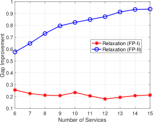
Figure 6: The average relative optimality gap improvement of relaxation (FP-I) and (FP-II).

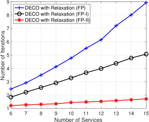
Figure 7: The average number of iterations needed by DECOs with relaxations (FP), (FP-I), and (FP-II), respectively.

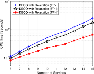
Figure 8: The average CPU time taken by DECOs with relaxations (FP), (FP-I), and (FP-II), respectively.

Fig. 6 plots the average gap improvement versus different numbers of services. As can be observed in Fig. 6, in all cases, the gap improvement is larger than $0.1$, which shows that (FP-I) and (FP-II) are indeed stronger than (FP). Compared with that of (FP-I), the gap improvement of (FP-II) is much larger. This indicates that the link-capacity based inequalities (26)–(31) can indeed significantly strengthening the FP problem only with the connectivity based inequalities (17) and (19). In addition, with the increasing of the number of services, the gap improvement of (FP-II) becomes larger. This can be explained as follows. As the number of services increases, the left-hand sides of inequalities (30) and (31) become larger, thereby making inequalities (30) and (31) tighter. Consequently, the gap improvement achieved by the link-capacity based inequalities is also likely to be larger.

Next, we illustrate the efficiency of the proposed connectivity based inequalities (17) and (19) and link-capacity based inequalities (26)–(31) for accelerating the convergence of the decomposition algorithm (called DECO). Figs. 7 and 8 plot the average numbers of iterations and CPU times needed by the proposed DECOs with relaxations (FP), (FP-I), and (FP-II), respectively, to terminate. As observed, both of the derived families of valid inequalities can improve the performance of the proposed DECO. In particular, with the two proposed inequalities, the average number of iterations needed for the convergence of DECO is much smaller (less than $2$); and thus the CPU time taken by DECO is also much smaller.

From the above computational results, we can conclude that the proposed DECO with relaxation (FP-II) (i.e., the FP problem with the two families of valid inequalities) significantly outperforms that with relaxation (FP) (i.e., the FP problem without the two families of valid inequalities). Due to this, we shall only test and compare the proposed DECO with relaxation (FP-II) with the other existing algorithms in the following.

V-B Comparison of DECO with SOTA Algorithms

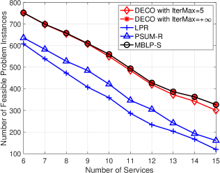
Figure 9: The number of feasible problem instances solved by DECOs with $\text{IterMax}=5,\,+\infty$, LPR, PSUM-R, and MBLP-S.

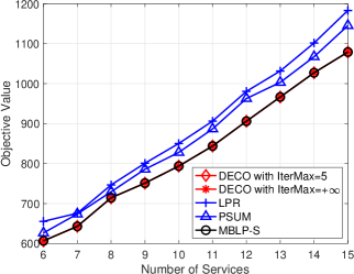
Figure 10: The average objective value returned by DECOs with $\text{IterMax}=5,\,+\infty$, LPR, PSUM-R, and MBLP-S.

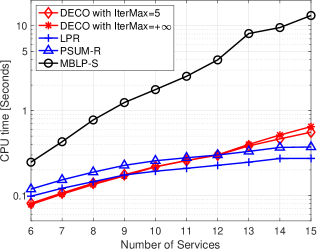
Figure 11: The average CPU time returned by DECOs with $\text{IterMax}=5,\,+\infty$, LPR, PSUM-R, and MBLP-S.

In this subsection, we compare the performance of the proposed DECO with SOTA algorithms such as the exact approach using standard MBLP solvers (called MBLP-S) in [7], the LP rounding (LPR) algorithm in [16], and the penalty successive upper bound minimization with rounding (PSUM-R) algorithm in [17].

Figs. 9 and 10 plot the number of feasible problem instances and the average objective value returned by the proposed DECOs with $\text{IterMax}=5,\,+\infty$, LPR, PSUM-R, and MBLP-S, respectively. When setting $\text{IterMax}=5$, the proposed DECO cannot be guaranteed to find an optimal solution of problem (NS), and the red-diamond curve in Fig. 9 is obtained as follows: for a problem instance, if the proposed DECO can find an optimal solution of problem (NS) within 5 iterations, it is counted as a feasible instance; otherwise, it is infeasible. From Figs. 9 and 10, we can observe the effectiveness of the proposed DECOs over LPR and PSUM-R. In particular, compared with LPR and PSUM-R, the proposed DECOs can find a feasible solution for much more problem instances and return a much better solution with a much smaller objective value. The latter is reasonable, as stated in Theorem 3, DECOs must return an optimal solution as long as they find a feasible solution. Another simulation finding is that with the increasing of IterMax, DECO can return a feasible solution for more problem instances. Nevertheless, when $\text{IterMax}=5$, DECO can return a feasible solution for almost all instances (as DECO with $\text{IterMax}=+\infty$ is able to find all truly feasible problem instances and the difference between the numbers of feasible problem instances solved by DECOs with $\text{IterMax}=5$ and $\text{IterMax}=+\infty$ is small in Fig. 9). This shows that in most cases, DECO can return an optimal solution within a few number of iterations, thanks to the two derived families of valid inequalities.

The comparison of the solution efficiency of the proposed DECOs with $\text{IterMax}=5,\,+\infty$, LPR, PSUM-R, and MBLP-S is plotted in Fig. 11. We can observe from Fig. 11 that though both MBLP-S and the proposed DECO with $\text{IterMax}=+\infty$ can return an optimal solution (if the problem is feasible), DECO with $\text{IterMax}=+\infty$ is much more computationally efficient than MBLP-S. In particular, the average CPU times taken by DECO with $\text{IterMax}=+\infty$ are less than $0.7$ seconds, while the CPU times taken by MBLP-S in the large-scale cases (i.e., $|\mathcal{K}|\geq 13$) are generally larger than $5$ seconds. The solution efficiency of the proposed DECO with $\text{IterMax}=5$, LPR, and PSUM-R is comparable. In general, LPR performs the best in terms of the CPU time, followed by DECO with $\text{IterMax}=5$ and PSUM-R.

In summary, our simulation results show both of the effectiveness and efficiency of the proposed DECO. More specifically, compared with the LPR and PSUM-R algorithms in [16] and [17], the proposed DECO is able to find a much better solution (due to the information feedback between the two subproblems); compared with the exact approach in [7], the proposed DECO is significantly more computationally efficient, which is because of its decomposition nature.

VI Conclusions

In this paper, we have proposed an efficient decomposition algorithm for solving large-scale NS problems. The proposed algorithm decomposes the large-scale NS problem into two relatively easy FP and TR subproblems and solves them in an iterative fashion enabling a useful information feedback between them (to deal with the coupled constraints) until an optimal solution of the problem is found. To further improve the efficiency of the proposed decomposition algorithm, we have also developed two families of valid inequalities to speed up its convergence by judiciously taking the special structure of the considered problem into account. Two key features of the proposed algorithm, which make it particularly suitable to solve the large-scale NS problems, are as follows. First, it is guaranteed to find an optimal solution of the NS problem if the number of iterations between the two subproblems is allowed to be sufficiently large and it can return a much better solution than existing two-stage heuristic algorithms even though the number of iterations between the subproblems is small (e.g., 5). Second, the FP and TR subproblems in the proposed decomposition algorithm are a small MBLP problem and a polynomial time solvable LP problem, respectively, which are much easier to solve than the original problem. Simulation results show the effectiveness and efficiency of the proposed decomposition algorithm over the existing SODA algorithms in [7, 16, 17]. In particular, when compared with algorithms based on LP relaxations [16, 17], the proposed decomposition algorithm is able to find a much better solution; when compared with the algorithm needed to call MBLP solvers [7], the proposed decomposition algorithm is much more computationally efficient.

Appendix A Proof of Theorem 5

Since inequalities (17)–(18) include inequalities (14)–(16), it follows that $\mathcal{X}^{2}\subseteq\mathcal{X}^{1}$ and $\mathcal{X}_{{\text{L}}}^{2}\subseteq\mathcal{X}_{{\text{L}}}^{1}$. Next, we prove $\mathcal{X}^{3}\subseteq\mathcal{X}^{2}$ and $\mathcal{X}_{{\text{L}}}^{3}\subseteq\mathcal{X}_{{\text{L}}}^{2}$. First, adding (19) for all $s^{\prime}=s,\ldots,s_{0}-1$ ($s_{0}\geq s+1$) yields

$$\sum_{s^{\prime}=s}^{s_{0}-1}\sum_{v\in\mathcal{V}\backslash\mathcal{V}(v_{0})}x^{k,s^{\prime}}_{v}\leq\sum_{s^{\prime}=s}^{s_{0}-1}\sum_{v\in\mathcal{V}\backslash\mathcal{V}(v_{0})}x_{v}^{k,s^{\prime}+1},$$

which is equivalent to

$$\sum_{v\in\mathcal{V}\backslash\mathcal{V}(v_{0})}x^{k,s}_{v}\leq\sum_{v\in\mathcal{V}\backslash\mathcal{V}(v_{0})}x_{v}^{k,s_{0}}.$$ (36)

By (1), we have

$$\sum_{v\in\mathcal{V}}x_{v}^{k,s_{0}}=1.$$ (37)

Combining (36) and (37) shows

$$\sum_{v\in\mathcal{V}\backslash\mathcal{V}(v_{0})}x^{k,s}_{v}+\sum_{v\in\mathcal{V}(v_{0})}x_{v}^{k,s_{0}}\leq 1.$$ (38)

By the definition of $\mathcal{V}(v_{0})$ in (13), we have $v_{0}\in\mathcal{V}\backslash\mathcal{V}(v_{0})$. As a result, (38) implies (18), which shows $\mathcal{X}^{3}\subseteq\mathcal{X}^{2}$ and $\mathcal{X}_{{\text{L}}}^{3}\subseteq\mathcal{X}_{{\text{L}}}^{2}$.

To show the theorem, it suffices to prove $\mathcal{X}^{1}\subseteq\mathcal{X}^{3}$. Next, we show the desirable result via verifying that (17) and (19) hold for any $\bm{x}\in\mathcal{X}^{1}$. We first show that (17) for $k\in\mathcal{K}$, $v\in\mathcal{V}(S^{k})$, and $s\in\mathcal{F}^{k}$ hold at $\bm{x}$ by an induction of $s$. By (14), $x_{v}^{k,s}=0$ holds for $s=1$. Suppose that $x_{v}^{k,s}=0$ holds for $s=1,2,\ldots,s_{0}$ ($1\leq s_{0}<\ell_{k}$). Then we have $x_{v}^{k,s_{0}}=0$ for all $v\in\mathcal{V}(S^{k})$. This, together with (1), implies

$$\sum_{v\in\mathcal{V}\backslash\mathcal{V}(S^{k})}x_{v}^{k,s_{0}}=1.$$ (39)

By (16), we have

$$x_{v_{0}}^{k,s_{0}}+x_{v}^{k,s_{0}+1}\leq 1,~{}\forall~{}v_{0}\in\mathcal{V}\backslash\mathcal{V}(S^{k}),~{}\forall~{}v\in\mathcal{V}(v_{0}).$$ (40)

Combining the above with (39) and the fact that $x_{v_{0}}^{k,s_{0}}\in\{0,1\}$ for all $v_{0}\in\mathcal{V}\backslash\mathcal{V}(S^{k})$ gives

$$x_{v}^{k,s_{0}+1}=0,~{}\forall~{}v\in\bigcap_{v_{0}\in\mathcal{V}\backslash\mathcal{V}(S^{k})}\mathcal{V}(v_{0}).$$ (41)

By Proposition 4 (ii), $\mathcal{V}(S^{k})\subseteq\mathcal{V}(v_{0})$ must hold for all $v_{0}\in\mathcal{V}\backslash\mathcal{V}(S^{k})$. Hence, we have

$$\mathcal{V}(S^{k})\subseteq\bigcap_{v_{0}\in\mathcal{V}\backslash\mathcal{V}(S^{k})}\mathcal{V}(v_{0}).$$

Together with (41), this implies that $x_{v}^{k,s_{0}+1}=0$ holds for all $v\in\mathcal{V}(S^{k})$.

Next, we show that (17) holds for all $k\in\mathcal{K}$, $v\in\mathcal{V}(D^{k})$, and $s\in\mathcal{F}^{k}$ at $\bm{x}\in\mathcal{X}^{1}$ by an induction of $s$. By (15), $x_{v}^{k,s}=0$ holds for $s=\ell_{k}$. Suppose that $x_{v}^{k,s}=0$ holds for $s=s_{0},s_{0}+1,\ldots,\ell_{k}$, where $1<s_{0}\leq\ell_{k}$. Then we have $x_{v}^{k,s_{0}}=0$ for all $v\in\mathcal{V}(D^{k})$. This, together with (1), implies

$$\sum_{v\in\mathcal{V}\backslash\mathcal{V}(D^{k})}x_{v}^{k,s_{0}}=1.$$ (42)

By (16), we have

$$x_{v_{0}}^{k,s_{0}-1}+x_{v}^{k,s_{0}}\leq 1,~{}\forall~{}v_{0}\in\mathcal{V}(D^{k}),~{}\forall~{}v\in\mathcal{V}(v_{0}).$$ (43)

From Proposition 4 (iii), $\mathcal{V}\backslash\mathcal{V}(D^{k})\subseteq\mathcal{V}(v_{0})$ holds for all $v_{0}\in\mathcal{V}(D^{k})$. This, together with (42), (43), and the fact that $x_{v_{0}}^{k,s_{0}}\in\{0,1\}$ for all $v_{0}\in\mathcal{V}\backslash\mathcal{V}(D^{k})$, implies that $x_{v_{0}}^{k,s_{0}-1}=0$ for all $v_{0}\in\mathcal{V}(D^{k})$.

Finally, we show that all inequalities in (19) hold at $\bm{x}\in\mathcal{X}^{1}$. By (1), we have

$$\sum_{v\in\mathcal{V}}x^{k,s+1}_{v}=1,$$ (44)

where $1\leq s<\ell_{k}$. For $v_{0}\in\mathcal{V}$, by $x_{v_{0}}^{k,s}\in\{0,1\}$ and $x_{v}^{k,s+1}\in\{0,1\}$ for $v\in\mathcal{V}(v_{0})$, (16), and (44), we have

$$x_{v_{0}}^{k,s}+\sum_{v\in\mathcal{V}(v_{0})}x^{k,s+1}_{v}\leq 1.$$ (45)

Combining (44) and (45) further yields

$$x_{v_{0}}^{k,s}\leq\sum_{v\in\mathcal{V}\backslash\mathcal{V}(v_{0})}x^{k,s+1}_{v}.$$ (46)

Similarly, for any $v^{\prime}\in\mathcal{V}\backslash\mathcal{V}(v_{0})$, we can show

$$x_{v^{\prime}}^{k,s}\leq\sum_{v\in\mathcal{V}\backslash\mathcal{V}(v^{\prime})}x^{k,s+1}_{v}\leq\sum_{v\in\mathcal{V}\backslash\mathcal{V}(v_{0})}x_{v}^{k,s+1},$$ (47)

where the last inequality follows from the fact that $\mathcal{V}(v_{0})\subseteq\mathcal{V}(v^{\prime})$ for all $v^{\prime}\in\mathcal{V}\backslash\mathcal{V}(v_{0})$, as stated in Proposition 4 (i). Now we can use $\sum_{v^{\prime}\in\mathcal{V}}x_{v^{\prime}}^{k,s}=1$ in (1), (47), and the binary natures of all variables $x_{v^{\prime}}^{k,s}\in\{0,1\}$ to conclude the desirable inequalities in (19).

Appendix B Details of Example 1

In this part, we show that for the toy example in Example 1, solving the LP relaxation of problem (FP) with (17) and (19) will return a solution with the objective value being $\frac{1}{4}$, and solving the LP relaxation of problem (FP) with (14)–(16) or (17)–(18) will return a solution with the objective value being $\frac{1}{6}$.

In this toy example, since there is only a single service, we let $x_{v}^{s}\in\{0,1\}$ denote whether function $f_{s}$ is allocated to cloud node $v$, where $v\in\{1,2,3\}$ and $s\in\{1,2\}$. Since the power consumption of activating cloud nodes is zero, we can, without loss of generality, set $y_{v}=1$ in problem (FP), and hence all constraints in (2) are redundant. In this case, the constraints in (1) reduce to

$$x_{1}^{1}+x_{2}^{1}+x_{3}^{1}=1,$$ (48)

$$x_{1}^{2}+x_{2}^{2}+x_{3}^{2}=1.$$ (49)

As $\mu_{1}=\mu_{2}=+\infty$, $\mu_{3}=3$, and $y_{1}=y_{2}=y_{3}=1$, the only effective constraint in (3) is

$$2x_{3}^{1}+2x_{3}^{2}\leq 3.$$ (50)

It is simple to check that $\mathcal{V}(S)=\mathcal{V}(D)=\emptyset$, $\mathcal{V}(1)=\emptyset$, $\mathcal{V}(2)=\{1\}$, and $\mathcal{V}(3)=\{1,2\}$, according to their definitions in (11)–(13). Since $\mathcal{V}(S)=\mathcal{V}(D)=\emptyset$, constraints in (14), (15), and (17) do not exist. As there are only two functions in the SFC of the service, constraints (16) and (18) are the same (meaning that problem (FP) with constraints (14)–(16) and that with (17)–(18) are also equivalent), which are

$$x_{2}^{1}+x_{1}^{2}\leq 1,$$ (51)

$$x_{3}^{1}+x_{1}^{2}\leq 1,$$ (52)

$$x_{3}^{1}+x_{2}^{2}\leq 1.$$ (53)

Finally, all constraints in (19) in this toy example read

$$x_{1}^{1}+x_{2}^{1}+x_{3}^{1}\leq x_{1}^{2}+x_{2}^{2}+x_{3}^{2},$$ (54)

$$x_{2}^{1}+x_{3}^{1}\leq x_{2}^{2}+x_{3}^{2},$$ (55)

$$x_{3}^{1}\leq x_{3}^{2}.$$ (56)

Therefore, the LP relaxation problem (FP) with (14)–(16) or (17)–(18) can be presented as

$$z_{{\text{LP}}_{1}}=\min_{\bm{x}}{} x_{1}^{1}+x_{2}^{1}$$ (57)

s. t. $$\eqref{cons1}\text{--}\eqref{exineq3},$$

$$x_{v}^{s}\in[0,1],~{}\forall~{}v\in\{1,2,3\},~{}\forall~{}s\in\{1,2\},$$

and the LP relaxation problem (FP) with (17) and (19) can be presented as

$$z_{{\text{LP}}_{2}}=\min_{\bm{x}}{} x_{1}^{1}+x_{2}^{1}$$ (58)

s. t. $$\eqref{cons1}\text{--}\eqref{cons3},~{}\eqref{exineq4}\text{--}\eqref{exineq6},$$

$$x_{v}^{s}\in[0,1],~{}\forall~{}v\in\{1,2,3\},~{}\forall~{}s\in\{1,2\}.$$

Below we show that $z_{{\text{LP}}_{1}}=\frac{1}{6}$ and $z_{{\text{LP}}_{2}}=\frac{1}{4}$, separately.
$\bullet$ Proof of $z_{{\text{LP}}_{1}}=\frac{1}{6}$.
Let $\bar{\bm{x}}$ be given as

$$\bar{x}_{1}^{1}=\frac{1}{6},~{}\bar{x}_{2}^{1}=0,~{}\bar{x}_{3}^{1}=\frac{5}{6},~{}\bar{x}_{1}^{2}=\frac{1}{6},~{}\bar{x}_{2}^{2}=\frac{1}{6},~{}\bar{x}_{3}^{2}=\frac{2}{3}.$$

It is simple to check that $\bar{\bm{x}}$ is feasible to problem (57), and thus $z_{{\text{LP}}_{1}}\leq\frac{1}{6}$. It remains to show $x_{1}^{1}+x_{2}^{1}\geq\frac{1}{6}$ for any feasible solution $\bm{x}$ of (57). By carefully combining (50), (52), and (53), we have

$$7 \geq(2x_{3}^{1}+2x_{3}^{2})+2(x_{3}^{1}+x_{1}^{2})+2(x_{3}^{1}+x_{2}^{2})$$

$$=6x_{3}^{1}+2(x_{1}^{2}+x_{2}^{2}+x_{3}^{2})=6x_{3}^{1}+2,$$

where the last equality follows from (49). Hence, we have $x_{3}^{1}\leq\frac{5}{6}$, which, together with (48), implies $x_{1}^{1}+x_{2}^{1}\geq\frac{1}{6}$.
$\bullet$ Proof of $z_{{\text{LP}}_{2}}=\frac{1}{4}$.
Let $\hat{\bm{x}}$ be given as

$$\hat{x}_{1}^{1}=\frac{1}{4},~{}\hat{x}_{2}^{1}=0,~{}\hat{x}_{3}^{1}=\frac{3}{4},~{}\hat{x}_{1}^{2}=\frac{1}{4},~{}\hat{x}_{2}^{2}=0,~{}\hat{x}_{3}^{2}=\frac{3}{4}.$$

It is simple to check that $\hat{\bm{x}}$ is feasible to problem (58), and thus $z_{{\text{LP}}_{2}}\leq\frac{1}{4}$. It remains to show $x_{1}^{1}+x_{2}^{1}\geq\frac{1}{4}$ for any feasible solution $\bm{x}$ of (58). By (50) and (56), we have $3\geq 2x_{3}^{1}+2x_{3}^{2}\geq 2x_{3}^{1}+2x_{3}^{1}=4x_{3}^{1}$ and thus $x_{3}^{1}\leq\frac{3}{4}$, which, together with (48), implies $x_{1}^{1}+x_{2}^{1}\geq\frac{1}{4}$.

References

- [1] W.-K. Chen, Y.-F. Liu, R.-J. Zhang, Y.-H. Dai, and Z.-Q. Luo, “An efficient decomposition algorithm for large-scale network slicing,” in Proc. IEEE 24th International Workshop on Signal Processing Advances in Wireless Communications (SPAWC), Shanghai, China, Sep. 2023. [Online]. Available: https://arxiv.org/abs/2306.15247.
- [2] S. Vassilaras, et al., “The algorithmic aspects of network slicing,” IEEE Commun. Mag., vol. 55, no. 8, pp. 112-119, Aug. 2017.
- [3] G. Mirjalily and Z.-Q. Luo, “Optimal network function virtualization and service function chaining: A survey,” Chin. J. Electron., vol. 27, no. 4, pp. 704-717, Jul. 2018.
- [4] R. Mijumbi, et al., “Network function virtualization: State-of-the-art and research challenges,” IEEE Commun. Surv. Tut., vol. 18, no. 1, pp. 236-262, Firstquarter 2016.
- [5] A. Jarray and A. Karmouch, “Periodical auctioning for QoS aware virtual network embedding,” in Proc. IEEE 20th International Workshop on Quality of Service (IWQoS), Coimbra, Portugal, Jun. 2012, pp. 1-4.
- [6] B. Addis, D. Belabed, M. Bouet, and S. Secci, “Virtual network functions placement and routing optimization,” in Proc. IEEE 4th International Conference on Cloud Networking (CloudNet), Niagara Falls, Canada, Oct. 2015, pp. 171-177.
- [7] W.-K. Chen, Y.-F. Liu, A. De Domenico, Z.-Q. Luo, and Y.-H. Dai. “Optimal network slicing for service-oriented networks with flexible routing and guaranteed E2E latency,” IEEE Trans. Netw. Service Manag., vol. 18, no. 4, pp. 4337-4352, Dec. 2021.
- [8] A. De Domenico, Y.-F. Liu, and W. Yu, “Optimal virtual network function deployment for 5G network slicing in a hybrid cloud infrastructure,” IEEE Trans. Wirel. Commun., vol. 19, no. 12, pp. 7942-7956, Dec. 2020.
- [9] A. Jarray and A. Karmouch, “Decomposition approaches for virtual network embedding with one-shot node and link mapping,” IEEE/ACM Trans. Netw., vol. 23, no. 3, pp. 1012-1025, Jun. 2015.
- [10] N. Huin, B. Jaumard, and F. Giroire, “Optimal network service chain provisioning,” IEEE/ACM Trans. Netw., vol. 26, no. 3, pp. 1320-1333, Jun. 2018.
- [11] J. Liu, W. Lu, F. Zhou, P. Lu, and Z. Zhu, “On dynamic service function chain deployment and readjustment,” IEEE Trans. Netw. Service Manag., vol. 14, no. 3, pp. 543-553, Sep. 2017.
- [12] Q. Hu, Y. Wang, and X. Cao, “Resolve the virtual network embedding problem: A column generation approach,” in Proc. IEEE INFOCOM, Turin, Italy, Apr. 2013, pp. 410-414.
- [13] R. Mijumbi, J. Serrat, J. Gorricho, and R. Boutaba, “A path generation approach to embedding of virtual networks,” IEEE Trans. Netw. Service Manag., vol. 12, no. 3, pp. 334-348, Sep. 2015.
- [14] A. Gupta, B. Jaumard, M. Tornatore, and B. Mukherjee, “A scalable approach for service chain mapping with multiple SC instances in a wide-area network,” IEEE J. Sel. Areas Commun., vol. 36, no. 3, pp. 529-541, Mar. 2018
- [15] S. Yang, et al., “Delay-aware virtual network function placement and routing in edge clouds,” IEEE Trans. Mob. Comput., vol. 20, no. 2, pp. 445-459, Feb. 2021.
- [16] M. Chowdhury, M. R. Rahman, and R. Boutaba, “ViNEYard: Virtual network embedding algorithms with coordinated node and link mapping,” IEEE/ACM Trans. Netw., vol. 20, no. 1, pp. 206-219, Feb. 2012.
- [17] N. Zhang, et al., “Network slicing for service-oriented networks under resource constraints,” IEEE J. Sel. Areas Commun., vol. 35, no. 11, pp. 2512-2521, Nov. 2017.
- [18] W.-K. Chen, Y.-F. Liu, F. Liu, Y.-H. Dai, and Z.-Q. Luo, “Towards efficient large-scale network slicing: An LP dynamic rounding-and-refinement approach,” IEEE Trans. Signal Process., vol. 71, pp. 615-630, Feb. 2023.
- [19] M. Yu, Y. Yi, J. Rexford, and M. Chiang, “Rethinking virtual network embedding: Substrate support for path splitting and migration,” ACM SIGCOMM Comput. Commun. Rev., vol. 38, no. 2, pp. 17-29, Apr. 2008.
- [20] J. Lischka and H. Karl, “A virtual network mapping algorithm based on subgraph isomorphism detection,” in Proc. the 1st ACM Workshop on Virtualized Infrastructure Systems and Architectures (VISA), Barcelona, Spain, Aug. 2009, pp. 81-88.
- [21] Y. T. Woldeyohannes, A. Mohammadkhan, K. K. Ramakrishnan, and Y. Jiang, “ClusPR: Balancing multiple objectives at scale for NFV resource allocation,” IEEE Trans. Netw. Service Manag., vol. 15, no. 4, pp. 1307-1321, Dec. 2018.
- [22] J. W. Jiang, T. Lan, S. Ha, M. Chen, and M. Chiang, “Joint VM placement and routing for data center traffic engineering,” in Proc. IEEE INFOCOM, Orlando, USA, Mar. 2012, pp. 2876-2880.
- [23] L. Qu, C. Assi, K. Shaban, and M. J. Khabbaz, “A reliability-aware network service chain provisioning with delay guarantees in NFV-enabled enterprise datacenter networks,” IEEE Trans. Netw. Service Manag., vol. 14, no. 3, pp. 554-568, Sep. 2017.
- [24] M. C. Luizelli, L. R. Bays, L. S. Buriol, M. P. Barcellos, and L. P. Gaspary, “Piecing together the NFV provisioning puzzle: Efficient placement and chaining of virtual network functions,” in Proc. IFIP/IEEE International Symposium on Integrated Network Management (IM), Ottawa, Canada, May 2015, pp. 98-106.
- [25] A. Mohammadkhan, et al., “Virtual function placement and traffic steering in flexible and dynamic software defined networks,” in Proc. of IEEE International Workshop on Local and Metropolitan Area Networks (LANMAN), Beijing, China, Apr. 2015, pp. 1-6.
- [26] Z. Zhang, et al., “A unified enhanced particle swarm optimization-based virtual network embedding algorithm,” Int. J. Commun. Syst., vol. 26, pp. 1054-1073, Jan. 2012.
- [27] X. Li and C. Qian, “The virtual network function placement problem,” in Proc. of IEEE Conference on Computer Communications Workshops (INFOCOM WKSHPS), Hong Kong, China, May 2015, pp. 69-70.
- [28] M. Abu-Lebdeh, D. Naboulsi, R. Glitho, and C. W. Tchouati, “On the placement of VNF managers in large-scale and distributed NFV systems,” IEEE Trans. Netw. Service Manag., vol. 14, no. 4, pp. 875-889, Dec. 2017.
- [29] N. Promwongsa, et al., “Ensuring reliability and low cost when using a parallel VNF processing approach to embed delay-constrained slices,” IEEE Trans. Netw. Service Manag., vol. 17, no. 4, pp. 2226-2241, Oct. 2020.
- [30] M. Conforti, G. Cornuéjols, and G. Zambelli, Integer Programming. Cham, Switzerland: Springer, 2014.
- [31] Y. Zhang, et al., “StEERING: A software-defined networking for inline service chaining,” in Proc. 21st IEEE International Conference on Network Protocols (ICNP), Goettingen, Germany, Oct. 2013, pp. 1-10.
- [32] J. Halpern and C. Pignataro, “Service function chaining (SFC) architecture,” 2015. [Online]. Available: https://www.rfc-editor.org/rfc/pdfrfc/rfc7665.txt.pdf.
- [33] 3GPP TSG SA5, “TR 32.972, Telecommunication management, Study on system and functional aspects of energy efficiency in 5G networks,” Release 16, V. 16.1.0, Sep. 2019. [Online]. Available: http://www.3gpp.org/DynaReport/32972.htm.
- [34] G. B. Dantzig and M. N. Thapa, Linear Programming 1: Introduction. New York: Springer, 1997.
- [35] A. Ben-Tal and A. Nemirovski, Lectures on Modern Convex Optimization: Analysis, Algorithms, and Engineering Applications. Philadelphia, USA: Society for Industrial and Applied Mathematics, 2001.
- [36] B. Addis, G. Carello, and M. Gao. “On a virtual network functions placement and routing problem: Some properties and a comparison of two formulations,” Networks, vol. 75, pp. 158-182, Mar. 2020
- [37] J. P. Vielma, S. Ahmed, and G. Nemhauser, “Mixed-integer models for nonseparable piecewise-linear optimization: Unifying framework and extensions,” Oper. Res., vol. 58, no. 2, pp. 303-315, Mar.-Apr. 2010.
- [38] R. Fukasawa and M. Goycoolea, “On the exact separation of mixed integer knapsack cuts,” Math. Program., vol. 128, pp. 19-41, Jun. 2011.
- [39]