Learning-on-the-Drive:
Self-supervised Adaptation of Visual Offroad Traversability Models

Abstract

Autonomous off-road driving requires understanding traversability, which refers to the suitability of a given terrain to drive over. When offroad vehicles travel at high speed ($>10/$), they need to reason at long-range ($50$-$100$) for safe and deliberate navigation. Moreover, vehicles often operate in new environments and under different weather conditions. LiDAR provides accurate estimates robust to visual appearances, however, it is often too noisy beyond 30m for fine-grained estimates due to sparse measurements. Conversely, visual-based models give dense predictions at further distances but perform poorly at all ranges when out of training distribution. To address these challenges, we present ALTER, an offroad perception module that adapts-on-the-drive to combine the best of both sensors. Our visual model continuously learns from new near-range LiDAR measurements. This self-supervised approach enables accurate long-range traversability prediction in novel environments without hand-labeling. Results on two distinct real-world offroad environments show up to 52.5% improvement in traversability estimation over LiDAR-only estimates and 38.1% improvement over non-adaptive visual baseline.

I INTRODUCTION

Consider a robot driving fast in a forest, as in Figure 1. Autonomous off-road driving requires the ability to estimate traversability accurately to determine the suitability of a given terrain for a vehicle to drive over. The robot must differentiate between bushes that cannot be traversed, tall grass that can be traversed but poses a risk, and trails that are ideal for high-speed traversal in order to make intelligent navigation decisions. While offroad driving has demonstrated many successes in the past decade [1, 2, 3, 4], most efforts are limited to slow speeds lower than 5m/s and are carefully developed for particular scenarios.

Challenges arise as we increase the speed ($>10/$) and the variety of terrains an autonomous system must navigate. To tackle these challenges, an effective offroad perception system should possess three key properties:

1. Accurate at long-range When operating at a high speed, the vehicle requires accurate traversability estimates beyond reactive range ($>30$) for more deliberate and safe navigation.

2. Robust in unseen environments Off-road vehicles often operate in new environments, e.g., desert and forest, or with different weather conditions, e.g., sunny and cloudy.

3. Fine-grained prediction The complexity of offroad environments requires differentiating terrain beyond binary classifications of traversable or non-traversable. For example, differentiating between various traversable areas: medium-risk tall grass, and low-risk trail.

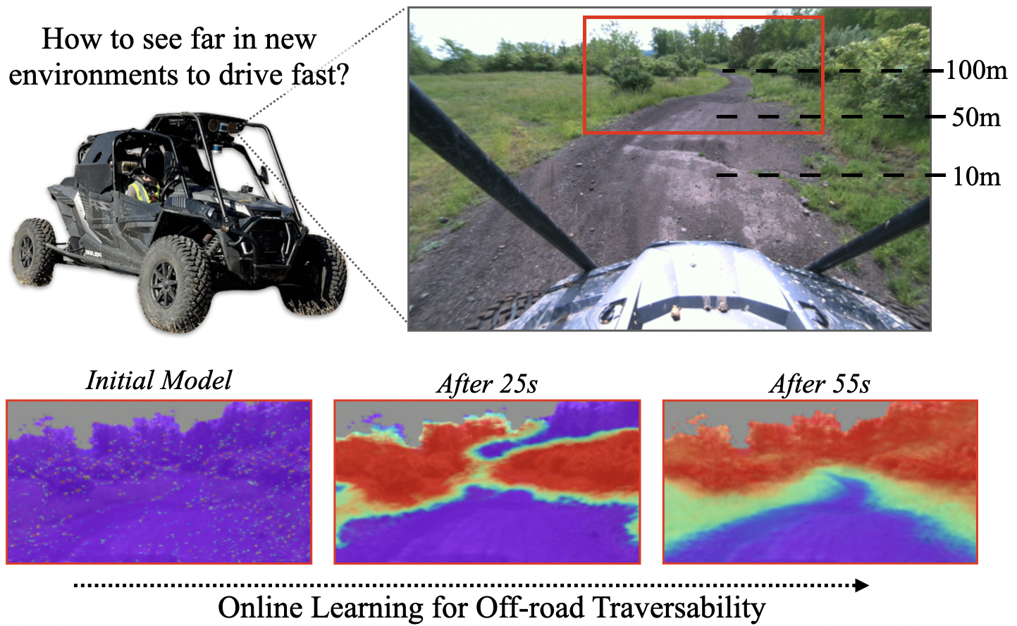
Figure 1: We present ALTER, an offroad perception framework that adapts on-the-drive to provide accurate long-range traversability prediction. We validate our adaptive method on two real-world offroad scenarios where it is able to differentiate between key terrains (trail, grass, obstacles) at a far distance with less than one minute of online learning.

Laser range sensors such as LiDAR are typically used to build a geometric understanding of the environment. Fine-grained traversability estimates can be generated by combining extracted LiDAR features, such as object height and smoothness [2, 5]. LiDAR provides accurate estimates robust to visual appearances, but its noise increases with range due to sparsity of points. On the contrary, camera-based methods output dense predictions at further distances [6, 7]. However, these models require a large human-annotated dataset and perform poorly when out of training distribution.

Online self-supervised techniques are used to adapt a visual model with appearance-invariant LIDAR measurements to leverage the benefits of both LiDAR and camera while remaining robust in unseen environments. However, prior LiDAR-based works either only produce binary traversable or non-traversable classification [8, 9, 10], or learn in colored point cloud space [11] which limits estimation to within reliable LiDAR range, limiting its long-range capability.

To simultaneously address the 3 needed properties, we present ALTER, Adaptive Long-range Traversibility EstimatoR. Our perception framework adapts its visual traversability model online using current LiDAR measurements to deliver accurate traversability estimates in unseen environments. By inferring in image space, our method produces pixel-wise traversability estimates that provide dense measurement at long-range. ALTER produces continuous-value traversability labels to provide fine-grained estimates needed for navigation. We present an example of offroad driving in Figure 1, where the vehicle can learn to differentiate between key terrains at a far distance with less than one minute of online learning.

Conceptually, we bridge the benefits of appearance-invariant LiDAR and dense camera measurements via online self-supervised learning. To label without manual annotation, we first accumulate near-range LiDAR information to build a large accurate long-range map, and then extract features from the accumulated map to label fine-grained traversability in 3D space. Lastly, we project the 3D labels to a previous image to produce dense long-range pixel-wise labels. During online learning, we continuously finetune a model with the latest self-labeled data to remain robust in unseen environments.

Our contributions are threefold:

1. To the best of our knowledge, we propose the first online learning framework to produce fine-grained, image-space traversability estimation supervised by LiDAR measurements. While the fine-grained or image-space estimation was independently explored, ours is the first to combine all elements to produce accurate long-range estimates that adapt to new environments.

2. We present a novel method to generate fine-grained and long-range pixel-wise traversability labels with LiDAR measurements. Previous works provide a binary traversability label, while we provide a continuous traversability score [8, 9]. In addition, the previous works use instantaneous LiDAR measurement to label which restricts the labeling range and accuracy. Our method uses accumulated LiDAR scans, extending the labeling range from 15 to 100.

3. We show, on 2 visually distinct environments, within 1 minute of combined data collection and training, our adaptive visual method produces up to 52.5% improvement in traversability estimation over LiDAR-only estimates and 34.3% improvement over visual models trained in another environment.

II RELATED WORKS

Traversability estimation: Traversability estimation involves understanding high-dimensional information to determine how suitable a specific terrain is for the vehicle to drive over. The two most common sensors for offroad perception are cameras and LiDARs. We find works that use LiDAR sensors to achieve this where a map is built with each grid cell containing some geometric statistics to help quantify traversability [12, 1, 5]. However, LiDAR measurements are sparse, and therefore noisy, at the distance. Many works therefore incorporate visual predictions to increase the range [4, 7]. For example, Maturana et al. [4] classifies an image into semantic classes, such as trail, grass, etc. However, these visual models are trained with a large amount of hand-annotated data and fail when deployed in environments different from the training distribution.

Cross-modal Self-supervised Learning: To alleviate the need for hard-to-acquire human annotation, self-supervised learning is often employed to generate labeled data automatically, with applications in natural language processing[13], healthcare[14], and robotics[15]. This paradigm lends itself well to combining complementary information across multiple sensors. Most related, we find successes in learning visual models with another sensor, for example, IMU[16, 17], force-torque signals [18], acoustic waveforms [19] and odometry [20, 21]. However, the above works rely on a static training dataset and may still fail when out of distribution.

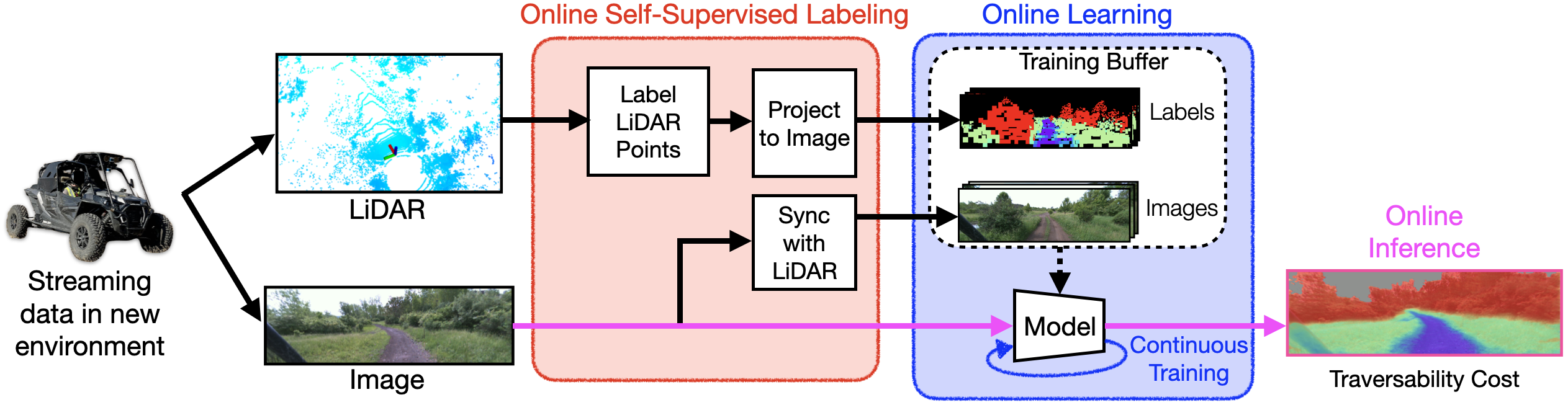
Figure 2: ALTER framework: Our adaptive approach estimates traversability from current images using models trained online with new LiDAR data. Online Labeling: We accumulate LiDAR scans and label in 3D their traversability costs given LIDAR features. The 3D labels are then projected onto the image plane to form training labels. Online Learning: ALTER continuously trains the model with the latest training buffer to adapt to new appearances. Online Inference: We predict pixel-wise fine-grained traversability scores for new images with the latest model.

Online Learning: Online learning investigates applications where the testing distribution is constantly changing by rapidly adapting to new data distributions. Common techniques include repeatedly training with the latest training buffer [22] or discarding outdated clusters of data [8]. More recently, with the rise of larger image datasets such as ImageNet [23], finetuning from pretrained model emerges as a more sample-efficient method for online learning [24]. However, fine-tuning a model on new tasks can lead to "forgetting" of previously learned information, known as catastrophic forgetting [25]. Continual learning approaches prevent forgetting by memory-based methods[26] and regularization-based methods [27].

Online Self-Supervised Learning for Traversability Estimation: For high-speed off-road driving, it is important to have accurate sensing at range even in new environments. We find multiple works that leverage cross-modal self-supervised learning and online learning to provide dense visual traversability estimation in unseen environments. Several works learn visual cues for traversability prediction by using stereo measurements as supervision[22, 28]. Hadsell et al. [22] segments camera images into multiple classes based on stereo-estimated object height. However, the authors also cite the unreliability of stereo range sensing to appearance and lighting changes as a key limitation.

Our work builds on successful approaches that adopt online self-supervised learning to combine LiDAR and cameras[8, 3, 11]. Sofman et al. [11] learns a mapping between LiDAR-based traversability to a colored point cloud space. However, the estimation is limited to within reliable LiDAR range, while our method can provide estimates beyond LiDAR sensing. We also find works that infer in image space [8, 9]. However, in both works, the prediction is limited to binary classes: traversable or non-traversable, which is overly conservative for the complex off-road environment. In contrast, our work provides a fine-grained traversability estimation. To address the limitations of past work, we seek to build an adaptive visual model that can learn from LiDAR measurements to provide fine-grained, pixel-wise predictions.

III APPROACH

III-A Overview

We aim to estimate fine-grained traversability at long-range while being robust to previously unseen environments. We achieve this by inferring in image space while adapting our visual model online with new LiDAR measurements.

As seen in Figure 2, ALTER is composed of three key steps:

1. Extracting image labels from accumulated LiDAR scans;

2. Training a visual model with the self-labeled data;

3. Infer on incoming images with online-learned models.

We describe each step in detail in the following subsections.

III-B Online Self-Supervised Labeling

We first generate pixel-wise traversability labels from current LiDAR measurements that will be used to adapt the visual models. Figure 3 describes the overall labeling process. Crucially, we generate the labels using accumulated near-range measurements to produce accurate long-range labels.

III-B1 Labeling in LiDAR Space

Accumulating LiDAR scans into voxel map

LiDAR scans (Figure 3a) are first registered with an IMU-based SLAM algorithm [29]. The resulting registered scans are then accumulated in a $120\times 120$ robot-centered 3D voxel map at 0.25 resolution.

Extracting LiDAR Features

We extract object height and planarity features from the accumulated map to inform traversability, with object height helping find large obstacles and planarity helping to differentiate between free space areas such as grass and trail. For object height $f_{\text{h}}$, we estimate the ground plane with a Markov Random Field-based Filter that interpolates between the heights of the neighboring lowest dense cells. For each voxel pillar, we label object height of each of its voxel by the difference between the height of tallest voxel and ground, as seen in Figure 3 (c).

On the other hand, for the planarity $f_{\text{p}}$, we calculate the eigenvalues for each top-down cell, by applying singular value decomposition on the aggregated LiDAR points in the cell. Using the eigenvalues, we calculate planarity by $\frac{(\lambda_{2}-\lambda_{3})\times 2}{\lambda_{1}}$. As seen in Figure 3 (c), planarity allows us to differentiate between trail/smooth ground (more planar) and grass/low vegetation (less planar) and is commonly used in offroad literatures[5, 30]. However, calculating planarity requires a high density of accurately registered points, which is significantly less likely at a distance, resulting in noisy far-range measurements. ALTER estimates in image space, therefore, produces accurate, long-range measurements.

Combining Features to Traversability Costs

We next combine the two LiDAR features into a continuous traversability score. To this end, we formulate a cost function that generally captures three terrain types of increasing severity: a trail that is low in height and high in planarity will be low cost, grass that is low in height and low in planarity will be medium cost, and untraversable obstacles that are above a height threshold are marked as high cost. We use the following cost function $J$, where $h_{\text{thresh}}=1$ is a threshold:

$$J(f_{\text{h}},f_{\text{p}})=\begin{cases}10&\text{if }f_{\text{h}}\geq h_{\text{thresh}}\\ 6-f_{\text{p}}\in[0,6]&\text{if }f_{\text{h}}<h_{\text{thresh}}\end{cases}$$ (1)

An example labeled 3D voxel map is shown in Figure 3 (d).

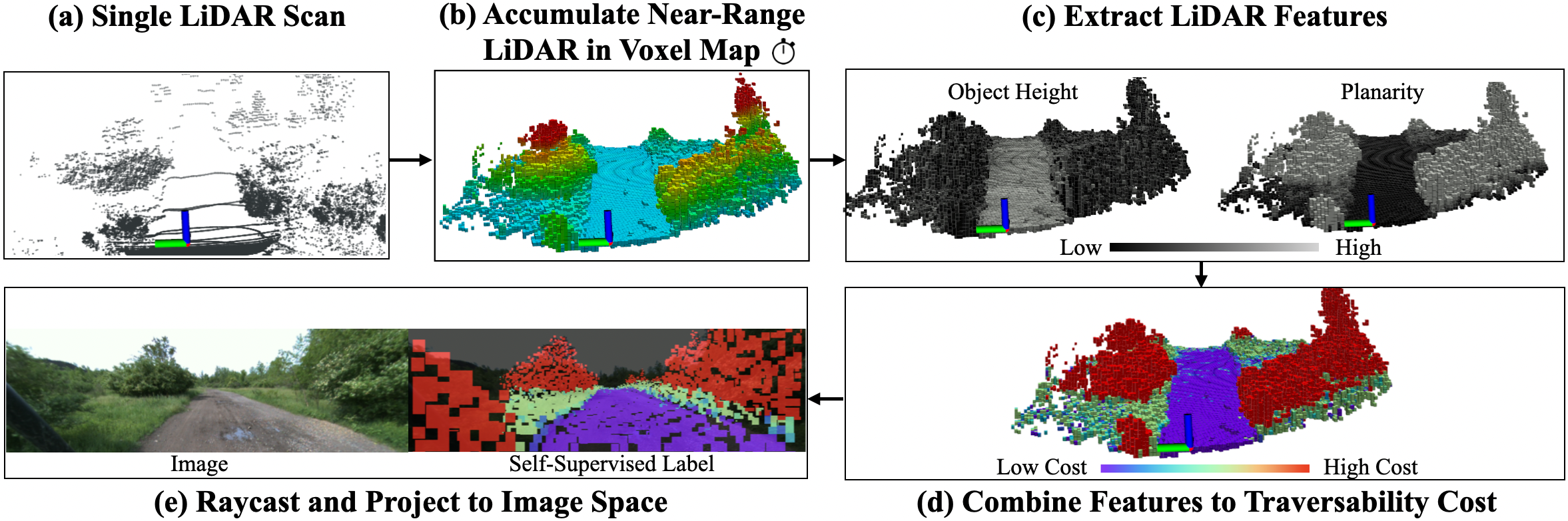
Figure 3: Self-Supervised Traversability Labeling Pipeline: Our self-supervised approach generates pixel-wise labels without manual labeling. First, LiDAR scans are registered and accumulated into a voxel map. Then, LiDAR features (object height, planarity) are extracted from the accumulated near-range map. Given a voxel’s LiDAR features, its traversability cost is calculated. Finally, the 3D labels are projected into image space to generate pixel-wise image labels. Our labels are able to distinguish between regions of different traversability, such as, trail, grass and tall obstacles, for visually distinct environments.

III-B2 Projecting LiDAR Labels to Image

Given labeled voxels in 3D space, we then project the information to image space to self-generate a pixel-wise label mask for visual traversability prediction. Figure 3(e) shows an example image, label pair.

Near-to-far projection

As described earlier, LiDAR measurements are often noisy at long ranges. To address the insufficient information at range, we perform a near-to-far learning similar to [31], which associates accumulated near-range measurements to supervise previous measurements. Specifically, we associate an image taken at time $t$ with a voxel map after a delay at $t+d$. The resulting labels are more accurate at farther range and cover a larger distance.

To capture accurate labels, we trim the admissible voxels to be within 15 of past and future robot odometries, within which LiDAR provides good estimates, and within 100m of the odometry at the image frame.

Raycasting from camera view

While projecting a future accumulated map improves the labeling accuracy, a naive projection of LiDAR labels will also include labels that would have been occluded from the initial viewpoint. To eliminate these labels, we perform Digital Differential Analysis (DDA)-style raycasting [32] starting from the image viewpoint at time $t$ into the voxel map at time $t+d$ to select suitable voxels to project. Finally, the four corners of each raycasted voxel surface closest to the camera $\mathbf{p}_{w}$ in world coordinates are projected to pixel positions in image coordinates $\mathbf{p}_{c}$ using a pinhole camera model, as follows: $\mathbf{p}_{c}=M_{\text{int}}\cdot M_{\text{ext}}\cdot\mathbf{p}_{w},$ where $M_{\text{int}}$ is the intrinsic matrix, $M_{\text{ext}}$ is the extrinsic matrix given by the odometry of the LiDAR sensor at time $t$. For each raycasted voxel surface, the enveloped space by its projected corners is filled in by the associated 3D traversability cost.

By labeling accumulated LiDAR measurement in a near-to-far manner, we can accurately label pixels up to 100m along the driven-over path, instead of just 15m. This results in more accurate and filled-out pixel-wise labels in image space.

III-C Online Learning

As new image/label pairs are generated from self-supervision, we continuously train models to adapt-on-the-drive to predict fine-grained pixel-wise traversability scores.

III-C1 Model Training

We use a U-Net model [33] as the base architecture with a MobileNet backbone [34] pretrained on ImageNet [23] to quickly adapt to changing environments. We train our model using a modified Mean Squared Error, that ignores unknown pixels, as the loss function between predicted values and self-supervised values. Due to dataset imbalance between different costs, we adjust the training loss to weigh pixels of different traversability costs using median frequency balancing[35]. To keep training time low, we train with a rolling buffer of 10 seconds with a frame per second, for 10 seconds. We use the top-half image to encourage the model to learn traversability at a distance.

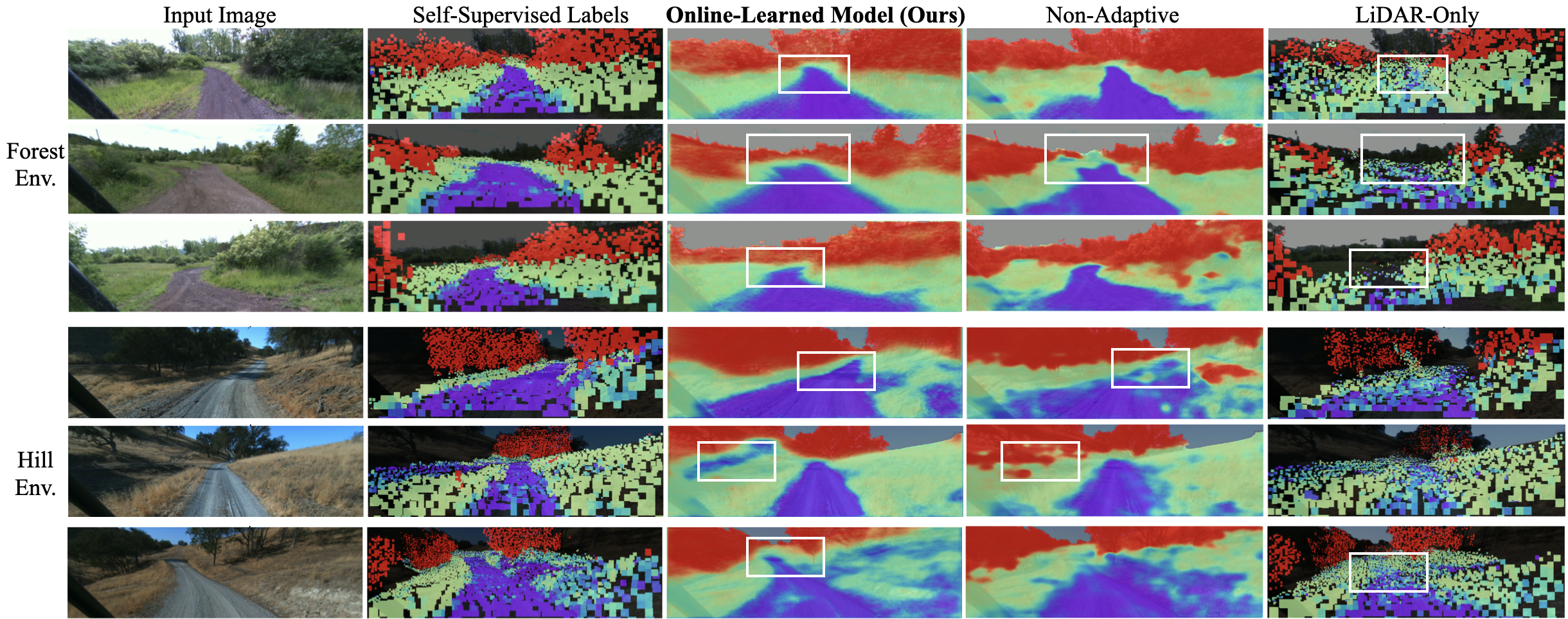
Figure 4: Qualitative results after 1 minute of adaptation: Our online-learned method is able to differentiate nuanced terrain (trail, grass, obstacle) at long-range within one minute of combined data collect and training. Compared to LiDAR-only baseline, our method is able to better differentiate grass and trail at the distance. Compared to a model pretrained on another environment, our adaptive method provides more robust predictions when deployed in a new environment.

III-C2 Continuous Model Selection

For more generalizable performance, we choose which model weights over a training cycle to deploy based on its performance in a wider validation buffer with older data. In this work, we choose 8 evenly-spaced frames, that does not overlap with training frames, from the latest 20 seconds of data as our validation buffer. During training, the best-performing model out of all epochs with respect to the validation buffer, is then used for inference and for continuous finetuning in the next training cycle.

III-D Online Traversability Inference

We infer on incoming images with our online-learned models using the top half of the image to focus on long-range predictions. For cleaner visualizations, we use an offroad segmentation model [36] to remove the sky.

IV RESULTS

We evaluate the robustness and adaptivity of ALTER on two real-world offroad datasets collected from distinct environments. Through our experiments, we aim to answer the following research questions:
Q1: Does adaptation enable more robust performance in new environments than pretrained visual models?
Q2: Does our visual model provide more accurate long-range perception than LiDAR-only estimates?
Q3: How do online learning parameters affect performance?
Q4: How do key design choices affect performance?
Q5: How does ALTER perform in previously-learned environment?

IV-A Data Collection

We use a Polaris RZR platform equipped with RGB cameras (Multisense S27) and LiDARs (Velodyne VLP-32C) as our data collection vehicle. We collect data in two visually distinct environments: forest and hill. The forest sequence was collected in a forest hill in Pittsburgh, PA with generally dark-green vegetation, green grass and some dark-brown colored trails. The hill sequence was collected in a hilly region in San Luis Obispo, CA featuring dry yellow grass with sparse trees. The images are acquired at 1024 $\times$ 750 pixels and downsampled to 512 $\times$ 384 pixels.

IV-B Baselines and Metrics

We compare our method with two baselines to compare its ability to capture traversability at range. The baselines represent the two paradigms that our method hopes to bridge:

1. LiDAR-only: the geometric traversability maps estimated with accumulated LiDAR points. For comparison, the estimated score are raycasted into image space.

2. Non-adaptive: the visual model trained in an environment other than the one we are testing on. We use a model trained with 50 epochs.

To compare the two methods, we calculate the mean square error (MSE) of the known pixels between the predicted image and the self-supervised labels. As the focus of this paper is long-range traversability estimates, we exclude points that are within 10 meters of the robot for comparison.

IV-C Comparison to baselines after 1 minute of adaptation

	Forest Env.		Hill Env.
Methods	MSE $\downarrow$	Difference from LiDAR $\downarrow$	MSE $\downarrow$	Difference from LiDAR $\downarrow$
ALTER (ours)	2.81$\pm$1.41	-52.5 %	3.81$\pm$2.98	-34.3 %
Non-adaptive	3.66$\pm$1.96	-38.1%	6.16$\pm$4.03	+6.1 %
LiDAR-only	5.92$\pm$1.38	-	5.80$\pm$1.35	-

TABLE I: Quantitative comparison to baselines after 1 minute of adaptation: We compare our online method to a LiDAR-only baseline and a visual model trained in another environment. Our adaptive approach provides more robustness to new environments than the baseline visual model. With less than a minute of data collection and training time, our model produces up to $52\%$ improvement over LIDAR.

Experimental Setup: We conduct simulated online experiments in the two environments to evaluate the performance of our adaptive method. In each environment, we use a 85 seconds sequence for training and inference, and we initialize the starting visual model with ImageNet[23] weights. Each of our training buffer contains 10 seconds of labeled image data. The labels are generated using a delayed projection of 5 seconds, meaning each label contains voxel information from time $t$ to $t+5$ seconds, where t is the image acquisition time. The model is allowed 10 seconds of training on each buffer before moving onto the next. This results in finishing training of the first model 25 seconds into the run and subsequent models trained in 10 seconds intervals. The self-supervised labels are preprocessed with a real-time implementation in progress. We train continuously for four models with a learning rate of $1e^{-3}$, ending the learning process at 55. The last 30 seconds (55-85 from start) are used as our test set. Table I quantitatively compares our online-learned method with the baselines, with our method providing more accurate long-range results after less than 1 minute of adaptation.

Does adaptation enable more robust prediction in new environments? After 55 seconds of data collection and training, our proposed method consistently outperforms the non-adaptive visual baseline, with up to 38.1% improvement. The experiment validates that adapting with self-supervised labels enables more robust performance in an out-of-distribution environment. Figure 4 shows representative qualitative outputs, where the online-learned module can clearly distinguish low-cost planar trails, medium-cost grassy regions and high-cost obstacles in both environments. In contrast, the baseline that is trained in different environments fails to generalize and often estimates trail region that is safe to traverse as medium-cost.

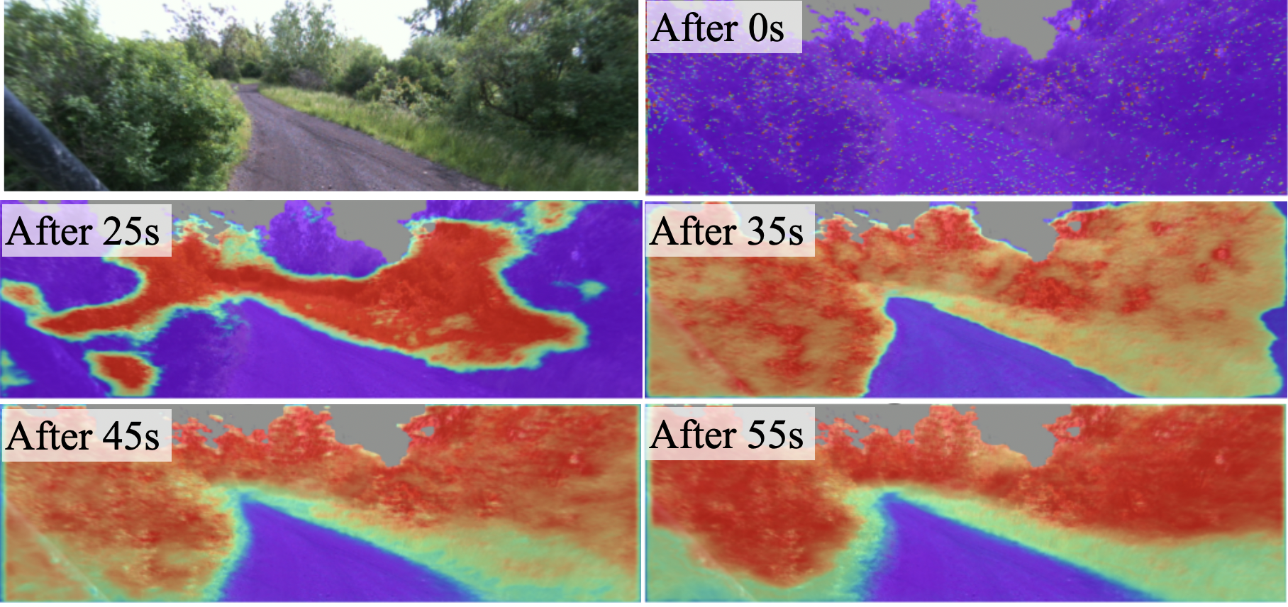
Figure 5: Model performance over time: We show the prediction on a held-out frame in Forest environment from the continuously-learning model. As expected, as more data is collected, model performance increases resulting in more fine-grained estimates with clearer boundaries at further terrain.

Figure 5 compares the performance of the continuously-learned models on the test set. As expected, error decreases with more training data and training time. While the first model (data collected and model trained within 35s) can discern the trail at close-range, it mislabels grass regions as having high cost. In general, we observe that the later models provide more fine-grained estimates and better boundary prediction between terrains.

Does the adapted visual model provide longer-range estimates? Additionally, we observe our adaptive visual prediction can provide more accurate traversability estimates than LiDAR at range, with up to a 52.5% reduction in error. In the first row of Figure 4, we show a scenario where our online-learned prediction differentiates the trail from the grass region at far-range, matching the self-supervised labels. In contrast, the map generated from LiDAR does not distinguish the two areas well as the planarity feature of the trail requires a high density of points to be accurate. Moreover, in the third row of Figure 4, the LiDAR-only baseline is unable to provide estimates on the trail at a distance as those cells do not yet have the required number of points. In contrast, our online-learned model is able to predict the trail and grass much further than even the general voxel map size.

IV-D Online Performance Analysis

We examine the online performance of our adaptive method and the impacts of online learning hyperparameters.

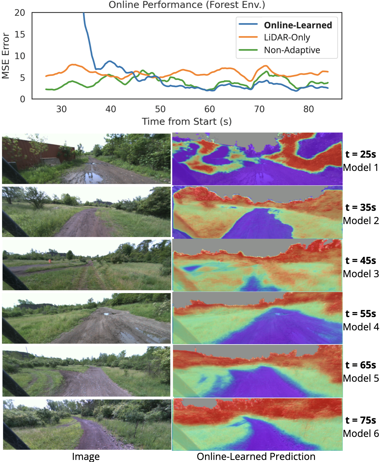
Figure 6: Online performance with our adaptive approach: Top: We compare our online method to baselines. For clearer visualization, we apply a moving average of 3 seconds. By 55 seconds from start, our adaptive visual model consistently provides better or comparable estimates compared to both baselines in both environments. Bottom: Over the test sequence, 6 models were trained starting from 25 and at 10 intervals. We show the first frame when a new model is deployed. As time increases, the performance improves. By 55 seconds, our model is able to differentiate between grass and trail at the distance, which a LiDAR-only method is not.

We leave our method to be fully adaptive throughout the sequence, with a starting model initialized with ImageNet weights. Figure 6 shows the online adaptive performance on the forest sequence, starting at 25 seconds when the first model is trained. By 55 seconds from the start (third model deployed, 30 seconds of data used), our adaptive visual model consistently provides better or comparable estimates compared to both baselines. In addition, we show the online prediction of the initial frame when a new model is deployed. By 55 seconds, we see our system has sufficiently adapted to the environment, able to provide good long-range fine-grained estimates.

We next quantify the impact of buffer length and learning rate on online performance.

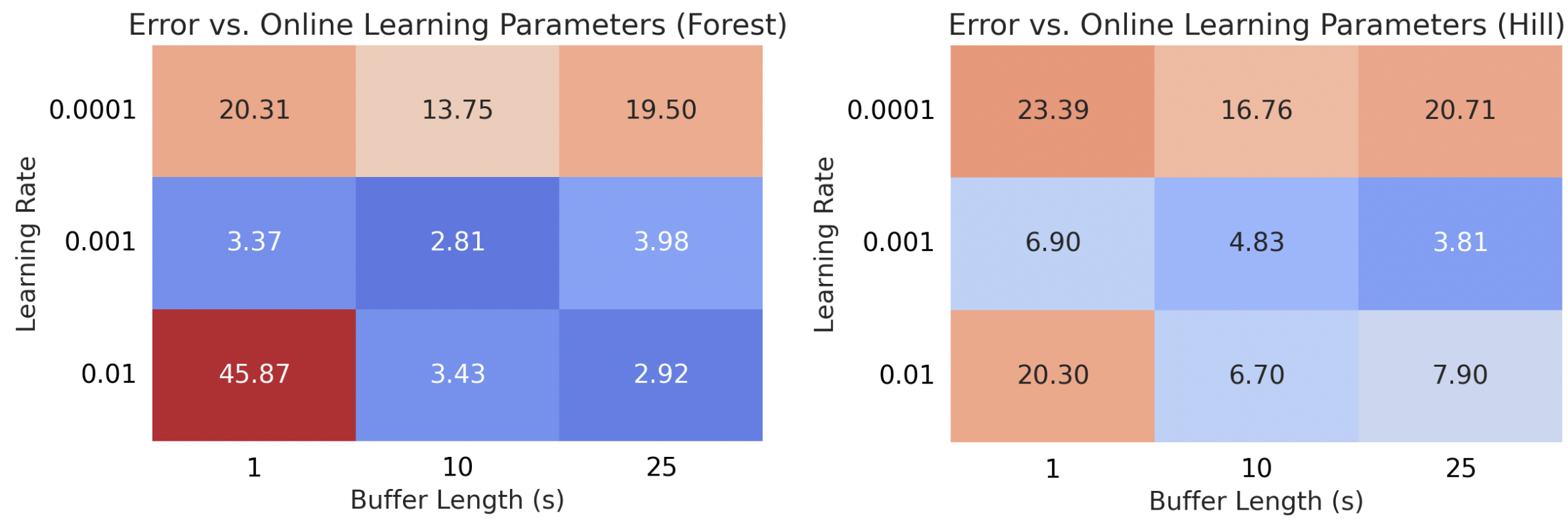
Figure 7: Average MSE given buffer length and learning rate: We find a buffer length of 10 seconds and a learning rate of $1e^{-3}$ to be optimal, providing a good tradeoff of reactivity and robustness.

Figure 7 shows the average error with various combinations of buffer length and learning rate. In both environments, we find a buffer length of 10 seconds and a learning rate of $1e^{-3}$ to be optimal for our application. We find that the highest errors occur when buffer length is 1 second. This is expected as the model may have overfitted to the very limited data. Alternatively, a buffer length of 25s is suboptimal as the latest model is effectively 30 seconds behind (25 training time, 5 accumulation time) the last data in the training buffer. Such a long delay does not allow for the reactivity needed for our application.

IV-E Ablation Studies

	Forest Env. MSE $\downarrow$	Hill Env. MSE $\downarrow$
Ours	2.81	4.83
w/o Accum	6.85	7.93
w/o Pretrain-ext	3.36	6.51

TABLE II: Ablation Studies of Key Modules: Average MSE loss in test set. We find learning with accurate labels (labeling with accumulated LiDAR scans) and learning with pretrained extractors to be critical for online performance.

Table II studies the relative impact of key design decisions to online performance. We investigate the impact of our accumulation of LiDAR scans for labeling (w/o Accum) and our use of a model with a pretrained ImageNet extractor (w/o Pretrain-ext). Similar to previous section, we apply our adaptive method throughout the entire sequence and report MSE error of the last 30 seconds of each sequence. As expected, learning from delayed accumulated LiDAR labels significantly improves performance as the training signal is denser and closer to ground truth. We then compare performance between initializing with a pretrained ImageNet extractor versus a random initialization (train from scratch). We find learning with the pretrained extractor also significantly improves adaptive performance.

Method	Training Sequence	Hill Env. MSE $\downarrow$	Forest Env. MSE$\downarrow$	Average MSE$\downarrow$
Ours	forest	18.9	2.81	10.85
Ours	hill	3.81	5.87	4.84
Ours	forest$\rightarrow$hill	4.02	4.50	4.26
Ours + EWC[27]	forest$\rightarrow$hill	4.12	3.52	3.82

TABLE III: Performance in Previously-Learned Environments: We continually adapt on forest and then hill sequence. Both variants of our method achieve better average performance when learned in both environments than with just one. Our method with EWC loss is able to better retain previous knowledge after learning in a new environment.

IV-F Performance in Previously-Learned Environment

We investigate how ALTER performs in previously-learned environments after learning in new environments, i.e., avoids catastrophic forgetting [25]. In our experiment, we first adapt a model to the forest sequence, then adapt to the hill sequence and evaluate the resulting model on the test sequences of both environments. We introduce an extension of our method to include Elastic Weight Consolidation (EWC) loss [27] (ours + EWC), which penalizes learning on weights important to previous tasks to limit forgetting. We set the EWC loss weight to $5e^{-3}$. Table III shows that after learning in the new hill environment, our methods (1 and 2 row) are still able to retain previous knowledge and achieve better performance in the forest environment compared to if they had not learned in it. By introducing EWC, we can better retain previous information, achieving the best average performance. Finally, we find that if it is possible to give our system one minute (an acceptable period for offroad driving) to adapt, resetting our model and learning solely in the test environment (3 and 4 row) performs best. Note that our model is also able to work with other lifelong/continual learning techniques such as [37], but it is out of the scope of this work.

V CONCLUSIONS

In this paper, we present ALTER, an offroad perception framework that adapts on-the-drive to provide accurate traversability prediction in novel environments. Central to this approach, is a self-supervised framework that adapts a visual model online with near-range LiDAR measurements. We validate with two offroad datasets that our adaptive visual method significantly increases robustness when operating in new environments. Within one minute of combined data collect and training, the model is able to differentiate between key terrains to provide fine-grained traversability estimates. We also show that the visual prediction is able to provide more accurate long-range measurements compared to LiDAR, especially on terrains that require dense points to differentiate.

We are interested in extending our adaptive perception framework in multiple directions. Instead of inferring only from images, we would like to learn a visual-lidar model online to leverage two sensors at inference time. We would also like to incorporate more LiDAR features such as, slope, density. Finally, we would like to incorporate more intelligent data sampling [38, 26].

References

- [1] D. Langer, J. Rosenblatt, and M. Hebert, “A behavior-based system for off-road navigation,” IEEE Transactions on Robotics and Automation, vol. 10, no. 6, pp. 776 – 783, December 1994.
- [2] A. Kelly, O. Amidi, M. Bode, M. Happold, H. Herman, T. Pilarski, P. Rander, A. Stentz, N. Vallidis, and R. Warner, “Toward reliable off road autonomous vehicles operating in challenging environments,” in Proceedings of 9th International Symposium on Experimental Robotics (ISER ’04), June 2004, pp. 599 – 608.
- [3] J. A. Bagnell, D. Bradley, D. Silver, B. Sofman, and A. Stentz, “Learning for autonomous navigation,” IEEE Robotics and Automation Magazine, vol. 17, no. 2, pp. 74–84, 2010.
- [4] D. Maturana, P.-W. Chou, M. Uenoyama, and S. Scherer, “Real-time semantic mapping for autonomous off-road navigation,” in Proceedings of 11th International Conference on Field and Service Robotics (FSR ’17), September 2017, pp. 335 – 350.
- [5] S. Triest, M. G. Castro, P. Maheshwari, M. Sivaprakasam, W. Wang, and S. Scherer, “Learning risk-aware costmaps via inverse reinforcement learning for off-road navigation,” 2023.
- [6] D. Maturana, P.-W. Chou, M. Uenoyama, and S. Scherer, “Real-time semantic mapping for autonomous off-road navigation,” in Field and Service Robotics. Springer, 2018, pp. 335–350.
- [7] T. Guan, D. Kothandaraman, R. Chandra, A. J. Sathyamoorthy, K. Weerakoon, and D. Manocha, “Ga-nav: Efficient terrain segmentation for robot navigation in unstructured outdoor environments,” IEEE Robotics and Automation Letters, vol. 7, no. 3, pp. 8138–8145, 2022.
- [8] H. Dahlkamp, A. Kaehler, D. Stavens, S. Thrun, and G. R. Bradski, “Self-supervised monocular road detection in desert terrain.” in Robotics: science and systems, vol. 38. Philadelphia, 2006.
- [9] D. Maier, M. Bennewitz, and C. Stachniss, “Self-supervised obstacle detection for humanoid navigation using monocular vision and sparse laser data,” in 2011 IEEE International Conference on Robotics and Automation. IEEE, 2011, pp. 1263–1269.
- [10] S. Zhou, J. Xi, M. W. McDaniel, T. Nishihata, P. Salesses, and K. Iagnemma, “Self-supervised learning to visually detect terrain surfaces for autonomous robots operating in forested terrain,” Journal of Field Robotics, vol. 29, no. 2, pp. 277–297, 2012.
- [11] B. Sofman, E. Lin, J. A. Bagnell, N. Vandapel, and A. Stentz, “Improving robot navigation through self-supervised online learning,” in Robotics: Science and Systems, 2006.
- [12] T. Overbye and S. Saripalli, “G-vom: A gpu accelerated voxel off-road mapping system,” in 2022 IEEE Intelligent Vehicles Symposium (IV), 2022, pp. 1480–1486.
- [13] J. Devlin, M.-W. Chang, K. Lee, and K. Toutanova, “BERT: Pre-training of deep bidirectional transformers for language understanding,” in Proceedings of the 2019 Conference of the North American Chapter of the Association for Computational Linguistics: Human Language Technologies, Volume 1 (Long and Short Papers). Minneapolis, Minnesota: Association for Computational Linguistics, June 2019, pp. 4171–4186.
- [14] E. Tiu, E. Talius, P. Patel, C. Langlotz, A. Ng, and P. Rajpurkar, “Expert-level detection of pathologies from unannotated chest x-ray images via self-supervised learning,” Nature Biomedical Engineering, vol. 6, pp. 1–8, 09 2022.
- [15] M. Sivaprakasam, S. Triest, W. Wang, P. Yin, and S. Scherer, “Improving off-road planning techniques with learned costs from physical interactions,” in 2021 IEEE International Conference on Robotics and Automation (ICRA). IEEE Press, 2021, p. 4844–4850.
- [16] M. Guaman Castro, S. Triest, W. Wang, J. M. Gregory, F. Sanchez, J. G. Rogers III, and S. Scherer, “How does it feel? self-supervised costmap learning for off-road vehicle traversability,” IEEE, 2023.
- [17] O. Mayuku, B. W. Surgenor, and J. A. Marshall, “A self-supervised near-to-far approach for terrain-adaptive off-road autonomous driving,” in 2021 IEEE International Conference on Robotics and Automation (ICRA), 2021, pp. 14 054–14 060.
- [18] L. Wellhausen, A. Dosovitskiy, R. Ranftl, K. Walas, C. Cadena, and M. Hutter, “Where should i walk? predicting terrain properties from images via self-supervised learning,” IEEE Robotics and Automation Letters, vol. 4, no. 2, pp. 1509–1516, 2019.
- [19] J. Zürn, W. Burgard, and A. Valada, “Self-supervised visual terrain classification from unsupervised acoustic feature learning,” IEEE Transactions on Robotics, vol. 37, no. 2, pp. 466–481, 2021.
- [20] R. Schmid, D. Atha, F. Schöller, S. Dey, S. Fakoorian, K. Otsu, B. Ridge, M. Bjelonic, L. Wellhausen, M. Hutter, and A.-a. Agha-mohammadi, “Self-supervised traversability prediction by learning to reconstruct safe terrain,” in 2022 IEEE/RSJ International Conference on Intelligent Robots and Systems (IROS), 2022, pp. 12 419–12 425.
- [21] X. Yao, J. Zhang, and J. Oh, “Rca: Ride comfort-aware visual navigation via self-supervised learning,” 2022.
- [22] R. Hadsell, A. Erkan, P. Sermanet, M. Scoffier, U. Muller, and Y. LeCun, “Deep belief net learning in a long-range vision system for autonomous off-road driving,” in 2008 IEEE/RSJ International Conference on Intelligent Robots and Systems. IEEE, 2008, pp. 628–633.
- [23] J. Deng, W. Dong, R. Socher, L.-J. Li, K. Li, and L. Fei-Fei, “Imagenet: A large-scale hierarchical image database,” in 2009 IEEE conference on computer vision and pattern recognition. Ieee, 2009, pp. 248–255.
- [24] K.-Y. Lee, Y. Zhong, and Y.-X. Wang, “Do pre-trained models benefit equally in continual learning?” in Proceedings of the IEEE/CVF Winter Conference on Applications of Computer Vision (WACV), January 2023, pp. 6485–6493.
- [25] R. M. French, “Catastrophic forgetting in connectionist networks,” Trends in Cognitive Sciences, vol. 3, no. 4, pp. 128–135, 1999.
- [26] C. de Masson d’Autume, S. Ruder, L. Kong, and D. Yogatama, “Episodic memory in lifelong language learning,” CoRR, vol. abs/1906.01076, 2019.
- [27] J. Kirkpatrick, R. Pascanu, N. Rabinowitz, J. Veness, G. Desjardins, A. A. Rusu, K. Milan, J. Quan, T. Ramalho, A. Grabska-Barwinska, D. Hassabis, C. Clopath, D. Kumaran, and R. Hadsell, “Overcoming catastrophic forgetting in neural networks,” Proceedings of the National Academy of Sciences, vol. 114, no. 13, pp. 3521–3526, 2017.
- [28] M. Happold, M. Ollis, and N. Johnson, “Enhancing supervised terrain classification with predictive unsupervised learning,” in Proceedings of Robotics: Science and Systems, Philadelphia, USA, August 2006.
- [29] S. Zhao, H. Zhang, P. Wang, L. Nogueira, and S. Scherer, “Super odometry: Imu-centric lidar-visual-inertial estimator for challenging environments,” in 2021 IEEE/RSJ International Conference on Intelligent Robots and Systems (IROS), 2021, pp. 8729–8736.
- [30] J.-F. Lalonde, N. Vandapel, D. F. Huber, and M. Hebert, “Natural terrain classification using three-dimensional ladar data for ground robot mobility,” Journal of Field Robotics, vol. 23, no. 10, pp. 839–861, 2006.
- [31] C. Wellington, A. Courville, and A. T. Stentz, “A generative model of terrain for autonomous navigation in vegetation,” The International Journal of Robotics Research, vol. 25, no. 12, pp. 1287–1304, 2006.
- [32] J. Amanatides and A. Woo, “A fast voxel traversal algorithm for ray tracing,” Proceedings of EuroGraphics, vol. 87, 08 1987.
- [33] O. Ronneberger, P. Fischer, and T. Brox, “U-net: Convolutional networks for biomedical image segmentation,” 2015.
- [34] A. G. Howard, M. Zhu, B. Chen, D. Kalenichenko, W. Wang, T. Weyand, M. Andreetto, and H. Adam, “Mobilenets: Efficient convolutional neural networks for mobile vision applications,” 2017, cite arxiv:1704.04861.
- [35] V. Badrinarayanan, A. Kendall, and R. Cipolla, “Segnet: A deep convolutional encoder-decoder architecture for image segmentation,” IEEE Transactions on Pattern Analysis and Machine Intelligence, vol. 39, no. 12, pp. 2481–2495, 2017.
- [36] Y. Yang, X. Meng, W. Yu, T. Zhang, J. Tan, and B. Boots, “Learning semantics-aware locomotion skills from human demonstration,” in Conference on Robot Learning. PMLR, 2023, pp. 2205–2214.
- [37] C. Wang, Y. Qiu, D. Gao, and S. Scherer, “Lifelong graph learning,” in IEEE/CVF Conference on Computer Vision and Pattern Recognition (CVPR), 2022.
- [38] C. Wang, Y. Qiu, W. Wang, Y. Hu, S. Kim, and S. Scherer, “Unsupervised online learning for robotic interestingness with visual memory,” IEEE Transactions on Robotics (T-RO), 2021.