A new classification framework for high-dimensional data

Abstract

Classification is a classic problem but encounters lots of challenges when dealing with a large number of features, which is common in many modern applications, such as identifying tumor sub-types from genomic data or categorizing customer attitudes based on on-line reviews. We propose a new framework that utilizes the ranks of pairwise distances among observations and identifies a common pattern under moderate to high dimensions that has been overlooked before. The proposed method exhibits superior classification power over existing methods under a variety of scenarios. Furthermore, the proposed method can be applied to non-Euclidean data objects, such as network data. We illustrate the method through an analysis of Neuropixels data where neurons are classified based on their firing activities. Additionally, we explore a related approach that is simpler to understand and investigates key quantities that play essential roles in our novel approach.

and

1 Introduction

In recent decades, the presence of high-dimensional data in classification is becoming more and more common. For example, gene expression data with thousands of genes was used to classify tumor sub-types (Golub et al., 1999; Ayyad, Saleh and Labib, 2019), on-line review data of hundreds of features was used to classify reviewers’ attitudes (Ye, Zhang and Law, 2009; Bansal and Srivastava, 2018), and speech signal data with thousands of utterances was used to classify speakers’ sentiment (Burkhardt et al., 2010). To address the challenges in classifying high-dimensional data, many methods have been proposed.

The support vector machine (SVM) was one of the early methods used for high-dimensional classification (Boser, Guyon and Vapnik, 1992; Brown et al., 1999; Furey et al., 2000; Schölkopf et al., 2001). Recently, Ghaddar and Naoum-Sawaya (2018) combined the SVM model with a feature selection approach to better handle high-dimensional data, and Hussain (2019) improved the traditional SVM by using a new semantic kernel. Linear discriminant analysis (LDA) is another commonly used method (Fisher, 1936; Rao, 1948), which has been extended to high-dimensional data by addressing the singularity of the covariance matrix, such as through generalized LDA (GLDA) (Li, Zhang and Jiang, 2005), dimension reduction with PCA and LDA in the low-dimensional space (Paliwal and Sharma, 2012), and regularized LDA (RLDA) (Yang and Wu, 2014). The $k$-nearest neighbor classification is also a common approach (Cover and Hart, 1967) with many variants (Liu et al., 2006; Tang et al., 2011). Recently, Pal, Mondal and Ghosh (2016) applied the $k$-nearest neighbor criterion based on a inter-point dissimilarity measure that utilizes the mean absolute difference to deal with the issue of the concentration of the pairwise distance. Other methods include the nearest centroids classifier with feature selection (Fan and Fan, 2008) and ensemble methods such as boosting and random forest (Freund et al., 1996; Buehlmann, 2006; Mayr et al., 2012; Breiman, 2001; Ye et al., 2013). In addition, neural network classification frameworks have shown promising results, particularly in image processing tasks, such as convolutional neural network and its variants (LeCun et al., 1989; Ranzato et al., 2006; Shi et al., 2015). There are also other methods available, such as partial least squares regression and multivariate adaptive regression splines, as reviewed in Fernández-Delgado et al. (2014).

While there are many methods for classification, a common idea in classification is that: the observations, or their projections are closer if they are from the same class. This rule works well when the dimension is low, but it could fail in some common scenarios for high-dimensional data. Consider a toy classification problem where the observations are from two distributions: $X_{1},X_{2},\dots,X_{50}\stackrel{{\scriptstyle\text{ i.i.d }}}{{\sim}}F_{X}$ and $Y_{1},Y_{2},\dots,Y_{50}\stackrel{{\scriptstyle\text{ i.i.d }}}{{\sim}}F_{Y}$. Here $F_{X}$ and $F_{Y}$ are unknown for classification, while $X_{1},X_{2},\dots,X_{50}$ and $Y_{1},Y_{2},\dots,Y_{50}$ are observed and labeled. The task is to classify a future observation, $W$, as belonging to either class $X$ or class $Y$. In this simulation, we set $X_{i}=\mathbf{A}(x_{i1},x_{i2},\dots,x_{id})^{\top}$, where $\mathbf{A}\in\mathbb{R}^{d\times d}$, $x_{ik}\stackrel{{\scriptstyle\text{ i.i.d }}}{{\sim}}t_{5}$, $d=1000$, $\mathbf{A}\mathbf{A}^{\top}=\Sigma$, with $\Sigma_{r,c}=0.1^{|r-c|}$ and $Y_{j}=\mathbf{B}(y_{j1},y_{j2},\dots,y_{jd})^{\top}+\mu$, $y_{ik}\stackrel{{\scriptstyle\text{ i.i.d }}}{{\sim}}t_{5}$, $\mathbf{B}\mathbf{B}^{\top}=a^{2}\Sigma$, $\mu=\mu_{0}\frac{\mu^{\prime}}{\|\mu^{\prime}\|}$, with $\mu^{\prime}$ is a random vector generated from $N_{d}(0,\mathbf{I}_{d})$. By setting different $\mu_{0}$’s and $a^{\prime}s$, the two distributions could vary in mean and/or variance. Fifty new observations are generated from each of the two distributions and are classified in each trial. The average misclassification rate is then calculated from fifty trials. While many classifiers are tested on this simple setting, we show results for a few representative ones from different categories that are either commonly used or show good performance: Generalized LDA (GLDA) (Li, Zhang and Jiang, 2005), supporter vector machine (SVM) (Schölkopf et al., 2001), random forest (RF) (Breiman, 2001), boosting (Freund et al., 1996), FAIR (Features Annealed Independence Rules) (Fan and Fan, 2008), NN-MADD ($k$-Nearest Neighbor classifier based on the Mean Absolute Difference of Distances) (Pal, Mondal and Ghosh, 2016), and several top rated methods based on the results in Fernández-Delgado et al. (2014) (decision tree (DT) (Salzberg, 1994), multivariate adaptive regression splines (MARS) (Leathwick et al., 2005) and partial least squares regression (PLSR) (Martens and Naes, 1992)).

Table 1: Misclassification rate (those smaller than ”the lowest misclassification rate $+\ 0.01$” are in bold).

$\mu_{0}$	$a$	GLDA	SVM	RF	Boosting	FAIR	NN-MADD	DT	MARS	PLSR
4	1	$\mathbb{0.243}$	$\mathbb{0.244}$	0.297	0.430	0.306	0.476	0.476	0.512	0.256
0	1.05	0.498	0.381	0.476	0.498	0.505	$\mathbb{0.357}$	0.532	0.524	0.480

Table 1 shows the average misclassification rate obtained from different classification methods when the mean or variance between the two distributions is different. When there is only mean difference, GLDA and SVM perform the best. When there is only variance difference, it turns out that NN-MADD performs the best. However, NN-MADD performs poorly when there is only mean difference. Therefore, there is a need to devise a new classification rule that works more universally.

The organization of the rest of the paper is as follows. In Section 2, we investigate the above toy example in more detail and propose a new classification approach that is capable of distinguishing between the two classes in both scenarios. In Section 3, we evaluate the performance of the new approach in various simulation settings, as well as in a real data application, where it outperforms existing methods. To gain a deeper understanding of the new method, Section 4 explores a related procedure that is simpler to handle and examines key quantities involved in the approach.

2 Method and theory

2.1 Intuition

It is well-known that, the equality of the two multivariate distributions $X\sim F$ and $Y\sim G$ can be characterized by the equality of three distributions – the distribution of the inter-point distance between two observations from sample $X$, the distribution of the inter-point distance between two observations from sample $Y$, and the distribution of the distance between one observation from sample $X$ and the other observation from sample $Y$ (Maa, Pearl and Bartoszyński, 1996). We ultilize the fact as the basis for our approach.

We begin by examining the inter-point distances of observations in both settings shown in Table 1. Heatmaps of these distances in a typical simulation run are shown in Figure 1 (top panel), where the data is arranged in the order of $X_{1},X_{2},\dots,X_{50}$ and $Y_{1},Y_{2},\dots,Y_{50}$. To see the patterns better, we also include in Figure 1 (bottom panel) data with larger differences: $\mu_{0}=15,a=1$ (left) and $\mu_{0}=0,a=1.15$ (right).

We denote the distance between two observations both from class $X$ as $D_{XX}$, the distance between one observation from class $X$ and the other from class $Y$ as $D_{XY}$, and the distance between two observations both from class $Y$ as $D_{YY}$. We see that, under the mean difference setting, the between group distance ($D_{XY}$) tend to be larger than the within group distance $(D_{XX},D_{YY})$ (left panel of Figure 1). Under the variance difference setting, where class Y has a larger variance difference, we see that $D_{XX}<D_{XY}<D_{YY}$ in general (right panel of Figure 1). This phenomenon is due to the curse of dimensionality, where the volume of the $d$-dimensional space increases exponentially in $d$, causing observations from a distribution with a larger variance to scatter far apart compared to those from a distribution with a smaller variance. This behavior of high-dimensional data has been discussed in Chen and Friedman (2017).

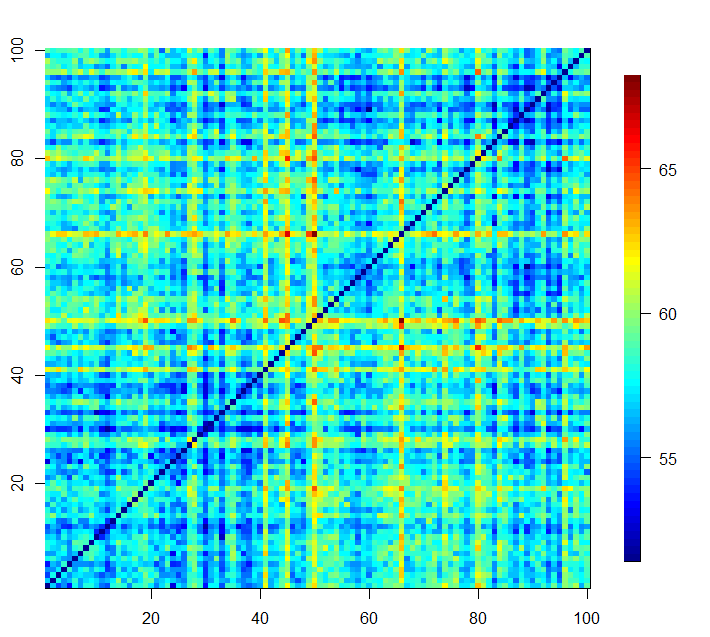
Figure 1: Heatmap of inter-point distances on observations generated from the two settings in Table 1 (top panel) and with larger differences (bottom panel).

Based on the above observations, we propose to use $(D_{XX},D_{XY})$ and $(D_{XY},D_{YY})$ as summary statistics for class $X$ and $Y$, respectively. Specially, under the mean difference setting, the between group distance ($D_{XY}$) tend to be larger than the within group distance $(D_{XX},D_{YY})$, so there are differences at both dimensions (the difference between $D_{XX}$ and $D_{XY}$ and the difference between $D_{XY}$ and $D_{YY}$); while under the variance difference setting, we have $D_{XX}<D_{XY}<D_{YY}$ (or $D_{XX}>D_{XY}>D_{YY}$ if class $X$ has a larger variance instead), so there are differences at both dimensions as well. In either scenario, the summary statistic is distinguishable between the two classes.

This idea can also be extended to solve $k$-class classification problem. For a $k$-class classification problem with class labels $1,2,\dots,k$, let $D_{ij}$ be the distance between one observation from the $i^{th}$ class and the other observation from the $j^{th}$ class and $D_{ii}$ be the inter-point distance between two observations from the $i^{th}$ class. We can use $D_{i}=(D_{i1},D_{i2},\dots,D_{ik})$ as the summary statistic for the $i^{th}$ class. For two class $i$ and $j$ differ in distribution, $(D_{ii},D_{ij})$ and $(D_{ij},D_{jj})$ also differ in distribution. Hence, the summary statistic $D_{i}$ could distinguish class $i$ from any classes.

After conducting extensive experiments, we found that using the pairwise distance directly is quite effective, but it is not robust to outliers (see Section 4.1). Therefore, we modify the approach by using ranks to make it more robust. We will revisit the distance-based version in Section 4 when we try to gain a better understanding of the approach.

2.2 Proposed method

Let $S=\left\{(Z_{i},g_{i}),i=1,2,\dots,N\right\}$ be a training set consisting of $N$ observations, where $Z_{i}\in\mathbb{R}^{d}$ represents the $i$-th observation and $g_{i}\in\left\{1,2,\dots,k\right\}$ is its corresponding label. We assume that all $Z_{i}$’s are independent and unique, and that if $g_{i}=j$, then $Z_{i}$ is drawn from the distribution $F_{j}$. Let $n_{j}=\sum_{i=1}^{N}\mathbbm{1}\left\{g_{i}=j\right\}$ denote the number of observations in the training set that belong to class $j$. The goal is to classify a new observation $W\in\mathbb{R}^{d}$ that is generated from one of the $k$ distributions $\left\{F_{j}\right\}_{j=1}^{k}$ to one of the $k$ classes.

Algorithm 1 Rank-based classification

• Construct a distance matrix $D\in\mathbb{R}^{N\times N}$, where $D[i,j]=\|Z_{i}-Z_{j}\|.$

• Construct a distance rank matrix $R\in\mathbb{R}^{N\times N}$, where $R[i,j]=\textit{the rank of}\ D[i,j]\ \textit{in the}\ j^{th}\ \textit{column}.$

• Construct a rank mean matrix $M\in\mathbb{R}^{N\times k}$:

  $$M[i,j]:=M_{j}(Z_{i})=\frac{1}{n_{j}-\mathbbm{1}\left\{g_{i}=j\right\}}\sum_{g_{l}=j,l\neq i}R[i,l].$$

• Construct a distance vector $D_{W}=(D_{W,1},D_{W,2},\dots D_{W,N})\in\mathbb{R}^{N}$, where $D_{W,i}=\|W-Z_{i}\|.$

• Construct a rank vector $R_{W}=(R_{W,1},R_{W,2},\dots R_{W,N})\in\mathbb{R}^{N}$, where

  $$R_{W,i}=\frac{1}{2}+\sum_{t=1}^{N}\mathbbm{1}\left\{\|Z_{t}-Z_{i}\|<\|W-Z_{i}\|\right\}+\frac{1}{2}\sum_{t=1}^{N}\mathbbm{1}\left\{\|Z_{t}-Z_{i}\|=\|W-Z_{i}\|\right\}.$$

• Construct a group rank vector $M_{W}=(M_{1}(W),M_{2}(W),\dots M_{k}(W))\in\mathbb{R}^{k}$, where

  $$M_{i}(W)=\frac{1}{n_{i}}\sum_{g_{l}=i}R_{W,l}.$$

• Use QDA to classify $M(W)$:

  $$g(W)=\arg\max_{j}\left\{-\frac{1}{2}\log|\hat{\Sigma}_{j}|-\frac{1}{2}(M_{W}-\hat{\mu}_{j})^{\top}\hat{\Sigma}_{j}^{-1}(M_{W}-\hat{\mu}_{j})+\log\frac{n_{j}}{N}\right\},$$

  where $\hat{\mu}_{j}=\frac{1}{n_{j}}\sum_{i=1}^{N}M_{j}(Z_{i})\mathbbm{1}\left\{g_{i}=j\right\}$, $\hat{\Sigma}_{j}=\frac{1}{n_{j}-1}\sum_{i=1}^{N}(M_{j}(Z_{i})-\hat{\mu}_{j})(M_{j}(Z_{i})-\hat{\mu}_{j})^{\top}\mathbbm{1}\left\{g_{i}=j\right\}.$

Remark 1.

In step 1, the distance could be the Euclidean distance or some other distances. In this paper, we use the Euclidean distance as the default choice. In step 7, the task is to classify $M_{W}$ based on all $M(Z_{i})^{\prime}s,i=1,2,\dots,N$. Since $M(w)$ is $k$-dimensional, where $k$ is the number of classes, other low-dimensional classification methods can also be used.

To illustrate how the first three steps do in separating the different classes, we plot the rank mean vector $M(Z_{i}),i=1,2,\dots,N$ for the four toy datasets in Figure 1. As shown in Figure 2, the classes are well separated, indicating the effectiveness of the first three steps.

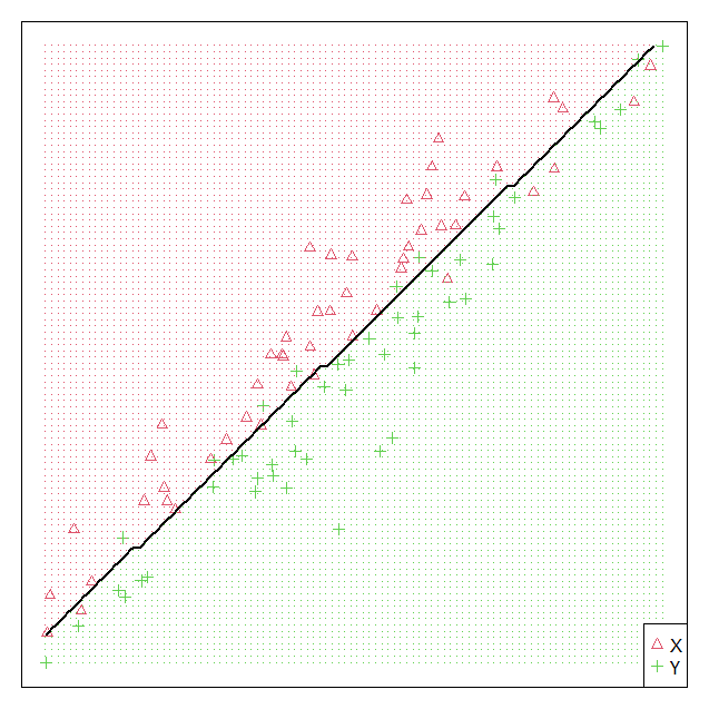
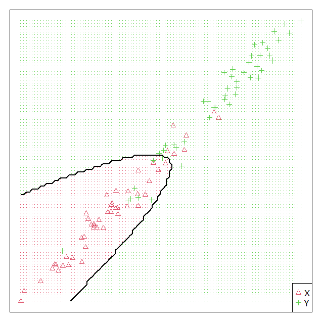
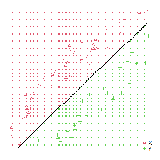
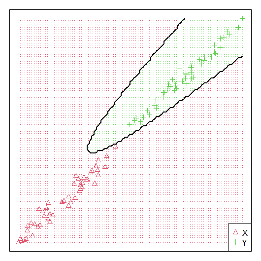
Figure 2: The scatter plot of the rank mean vector $M(\cdot)$ for the four datasets in Figure 1. The decision boundary is given by the quadratic discriminant analysis.

Table 2: Misclassification rate under the same settings as in Table 1

$\mu_{0}$	$a$	New	GLDA	SVM	RF	FAIR	NN-MADD	PLSR
4	1	$\mathbb{0.240}$	$\mathbb{0.243}$	$\mathbb{0.244}$	0.297	0.306	0.476	0.256
0	1.05	$\mathbb{0.282}$	0.498	0.381	0.476	0.505	0.357	0.480

We applied Algorithm 1 to the two scenarios described in Table 1, and the results are presented in Table 2. We see that, under the mean difference setting, the new method performs similarly to GLDA and SVM, which are the two best performers under this setting; and under the variance difference setting, the new approach outperforms all other methods.

3 Numerical studies

Here we examine the performance of the new method by comparing to other classification methods under more settings. Due to the fact that DT and MARS do not work well for either mean or variance differences, as indicated in Table 1, they are omitted in the following comparison.

3.1 Two-class classification

In each trial, we generate two independent samples, $X_{1},X_{2},\dots,X_{50}\stackrel{{\scriptstyle\text{ i.i.d }}}{{\sim}}F_{X}$ and $Y_{1},Y_{2},\dots,Y_{50}\stackrel{{\scriptstyle\text{ i.i.d }}}{{\sim}}F_{Y}$, with $X_{i}=\mathbf{A}(x_{i1},x_{i2},\dots,x_{id})^{\top}$, $x_{ik}\stackrel{{\scriptstyle\text{ i.i.d }}}{{\sim}}F_{x}$ and $Y_{j}=\mathbf{B}(y_{j1},y_{j2},\dots,y_{jd})^{\top}+\mu$, $y_{jk}\stackrel{{\scriptstyle\text{ i.i.d }}}{{\sim}}F_{y}$, to be the training set. We set $\mathbf{A}\mathbf{A}^{\top}=\Sigma$, with $\Sigma_{r,c}=0.1^{|r-c|}$, $d=1000$ , $\mathbf{B}=a\mathbf{A}$ and $\mu=\mu_{0}\frac{\mu^{\prime}}{\|\mu^{\prime}\|}$ with $\mu^{\prime}$ a random vector generated from $N_{d}(0,\mathbf{I}_{d})$. The testing samples are $W_{x_{1}},W_{x_{2}},\dots W_{x_{50}}\stackrel{{\scriptstyle\text{ i.i.d }}}{{\sim}}F_{X}$ and $W_{y_{1}},W_{y_{2}},\dots W_{y_{50}}\stackrel{{\scriptstyle\text{ i.i.d }}}{{\sim}}F_{Y}$. We consider a few different scenarios:

• Scenario 1: $F_{x}=N(0,1)$, $F_{y}=N(0,1)$;

• Scenario 2: $F_{x}=t_{5}$, $F_{y}=t_{5}$;

• Scenario 3: $F_{x}=\chi^{2}_{5}-5$, $F_{y}=\chi^{2}_{5}-5$;

• Scenario 4: $F_{x}=N(0,1)$, $F_{y}=t_{5}$.

Table 3 shows the average misclassification rate from $50$ trials. We see that, when there is only mean difference, the new method has close misclassfication rate to the best method among all other methods; when there is only variance difference, the new method perform the best among all the methods and only NN-MADD has close performance to the new method; when there are both mean and variance differences, the new method again has the lowest misclassification rate.

Table 3: Two-class misclassification rate

Scenario	$\mu_{0}$	$a$	New	GLDA	SVM	RF	Boosting	FAIR	NN-MADD	PLSR
Scenario 1	6	1	$\mathbb{0.027}$	$\mathbb{0.027}$	$\mathbb{0.023}$	0.115	0.354	0.077	0.343	$\mathbb{0.028}$
Scenario 1	0	1.1	$\mathbb{0.020}$	0.506	0.106	0.425	0.465	0.507	$\mathbb{0.025}$	0.412
Scenario 1	6	1.1	$\mathbb{0.003}$	0.044	$\mathbb{0.005}$	0.107	0.368	0.107	0.024	0.064
Scenario 2	6	1	0.109	$\mathbb{0.102}$	$\mathbb{0.092}$	0.161	0.385	0.170	0.476	0.116
Scenario 2	0	1.1	$\mathbb{0.100}$	0.483	0.172	0.424	0.473	0.493	0.145	0.536
Scenario 2	6	1.1	$\mathbb{0.042}$	0.128	$\mathbb{0.051}$	0.162	0.389	0.197	0.140	0.176
Scenario 3	6	1	0.414	$\mathbb{0.401}$	$\mathbb{0.399}$	$\mathbb{0.396}$	0.474	0.430	0.487	0.392
Scenario 3	0	1.1	$\mathbb{0.071}$	0.478	0.141	0.345	0.460	0.495	0.092	0.504
Scenario 3	6	1.1	$\mathbb{0.069}$	0.417	0.124	0.278	0.431	0.434	0.096	0.428
Scenario 4	0	1	$\mathbb{0.278}$	0.500	0.380	0.483	0.487	0.506	0.361	0.476

3.2 Multi-class classification

In each trial, we randomly generate $n=50$ observations from four distributions $Z_{ij}\stackrel{{\scriptstyle\text{ i.i.d }}}{{\sim}}F_{i},\ i=1,\dots,4$, $j=1,\dots,50$, to be the training set, with $Z_{ij}=a_{i}\mathbf{A}(z_{ij1},z_{ij2},\dots,z_{ijd})^{\top}+\mu_{i}$, $z_{ijk}\stackrel{{\scriptstyle\text{ i.i.d }}}{{\sim}}F_{z}$, $i=1,\dots,4$, $j=1,2,\dots,50$. We set $d=1000$, $\mathbf{A}\mathbf{A}^{\top}=\Sigma$, $\Sigma_{r,c}=0.1^{|r-c|}$ and $\mu=\mu_{0}\frac{\mu^{\prime}}{\|\mu^{\prime}\|}$, with $\mu^{\prime}$ a random vector generated from $N_{d}(0,\mathbf{I}_{d})$. The $a_{i}^{\prime}s$ and $\mu_{i}^{\prime}s$ are set as follow: $a_{1}=a_{3}=1$, $a_{2}=a_{4}=1.1$; $\mu_{1}=\mu_{2}=0$, $\mu_{3}=\mu_{4}=\mu$, $\mu_{0}=12$. Under those settings, the four distributions have two different means and two different variances. The testing samples are $W_{ij}\stackrel{{\scriptstyle\text{ i.i.d }}}{{\sim}}F_{i}$, $i=1,\dots,4$, $j=1,\dots,50$. We consider the following scenarios:

• Scenario 5: $F_{z}=N(0,1)$;

• Scenario 6: $F_{z}=t_{5}$;

• Scenario 7: $F_{z}=\chi^{2}_{5}-5$.

Table 4: Multi-class misclassification rate

Scenario	New	GLDA	SVM	RF	Boosting	NN-MADD	PLSR
Scenario 5	$\mathbb{0.023}$	0.495	0.118	0.444	0.502	0.640	0.498
Scenario 6	$\mathbb{0.133}$	0.495	0.190	0.456	0.513	0.603	0.506
Scenario 7	$\mathbb{0.216}$	0.584	0.306	0.482	0.583	0.696	0.505

The average misclassification rate of $50$ trials are shown in Table 4 (FAIR can only be applied to the two-class problem and is not included here). We see that, the new method has the lowest misclassification rate under all these scenarios.

3.3 Network data classification

We generate random graphs using the configuration model $G(v,\vec{k})$, where $v$ is the number of vertices and $\vec{k}$ is a vector containing the degrees of the $v$ vertices, with $k_{i}$ assigned to vertex $v_{i}$. In each trial, we generate two independent samples, $\left\{X_{1},X_{2},\dots,X_{30}\right\}$ and $\left\{Y_{1},Y_{2},\dots,Y_{30}\right\}$, with degree vectors $\vec{k}^{x}$ and $\vec{k}^{y}$, respectively. The testing samples are $W_{x_{1}},W_{x_{2}},\dots,W_{x_{20}}\stackrel{{\scriptstyle\text{ i.i.d }}}{{\sim}}G(v,\vec{k}^{x})$ and $W_{y_{1}},W_{y_{2}},\dots,W_{y_{20}}\stackrel{{\scriptstyle\text{ i.i.d }}}{{\sim}}G(v,\vec{k}^{y})$. We consider the following scenarios:

• Scenario 8: $k^{x}_{1}=k^{x}_{2}=\dots=k^{x}_{20}=1$, $k^{x}_{21}=k^{x}_{22}=\dots=k^{x}_{40}=3$; $k^{y}_{1}=k^{y}_{2}=\dots=k^{y}_{20-a}=1$, $k^{y}_{21-a}=k^{y}_{22-a}=\dots=k^{y}_{20}=2$, $k^{y}_{21}=k^{y}_{22}=\dots=k^{y}_{20+a}=4$, $k^{y}_{21+a}=k^{y}_{22+a}=\dots=k^{y}_{40}=3$;

• Scenario 9: $k^{x}_{1}=k^{x}_{2}=\dots=k^{x}_{40}=20$, $k^{y}_{1}=k^{y}_{2}=\dots=k^{y}_{40-a}=20$, $k^{y}_{41-a}=k^{y}_{42-a}=\dots=k^{y}_{40}=30$.

When comparing the performance of the methods, we convert the network data with 40 nodes into $40\times 40$ adjacency matrices, which are further converted into $1600$-dimensional vectors. We do this conversion so that all methods in the comparison can be applied. While for our approach, it can be applied to network data directly by using a distance on network data in step 1 of Algorithm 1.

The results are presented in Table 5. We see that the new method is among the best performers in all settings, while other good performers could work well under some settings but fail for others.

Table 5: Network data misclassification rate

Scenario	$a$	New	GLDA	SVM	RF	Boosting	NN-MADD	PLSR
Scenario 8	5	$\mathbb{0.054}$	0.377	0.382	0.405	0.445	0.119	0.318
Scenario 8	10	$\mathbb{0.011}$	0.342	0.321	0.371	0.462	$\mathbb{0.008}$	0.306
Scenario 8	15	$\mathbb{0.002}$	0.331	0.326	0.401	0.483	$\mathbb{0.001}$	0.376
Scenario 8	20	$\mathbb{0.000}$	0.315	0.290	0.380	0.470	$\mathbb{0.000}$	0.476
Scenario 9	4	$\mathbb{0.100}$	$\mathbb{0.090}$	0.151	0.220	0.404	0.386	0.254
Scenario 9	8	$\mathbb{0.007}$	$\mathbb{0.004}$	0.026	0.127	0.344	0.164	0.203
Scenario 9	12	$\mathbb{0.001}$	$\mathbb{0.004}$	$\mathbb{0.004}$	0.059	0.289	0.080	0.088
Scenario 9	16	$\mathbb{0.000}$	$\mathbb{0.001}$	$\mathbb{0.001}$	0.041	0.271	0.045	0.059

3.4 Real data analysis

We applied the new method to a neuropixels dataset (Stringer et al., 2019). The dataset comprises neural activity data for 1462 neurons across nine brain regions: Thalamus (TH), Midbrain (MB), Hippocampus (HPF), Superior colliculus (SC), V1, Front Motor (FrMo), Somatomotor (SomMo), Caudate putamen (CP), and Lateral septum (LS). The location of these brain regions are shown in Figure 3. We classified the neurons based on their firing activity data represented by 39053-length vectors.

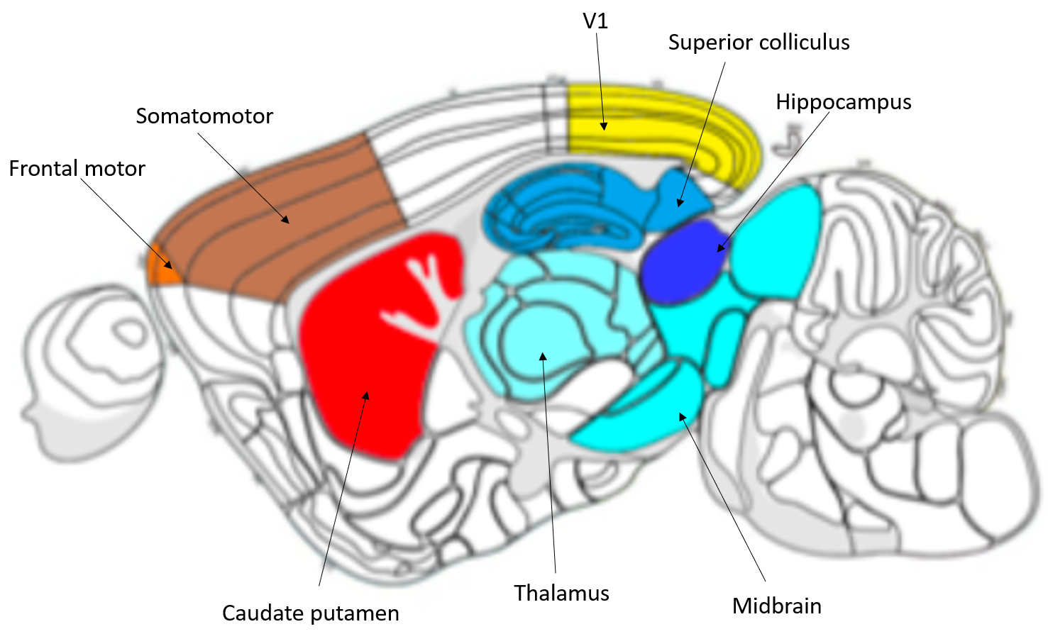
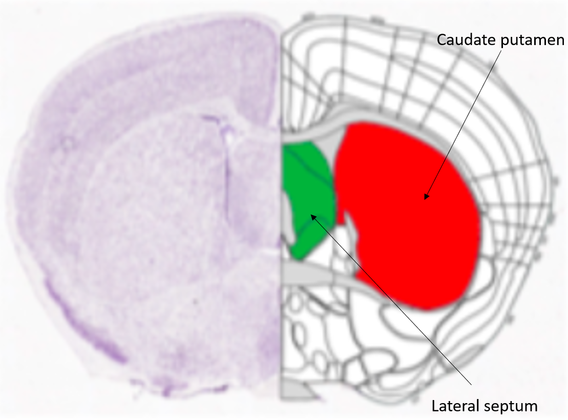
Figure 3: Mice brain atlases with sagittal view (left panel) and coronal view (right panel). This plot is adapted from Figure 3.B in (Chen, Chen and Deng, 2019).

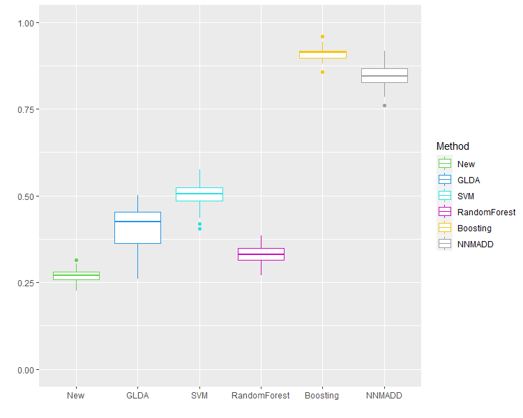
Figure 4: Misclassification rate on neuropixels data

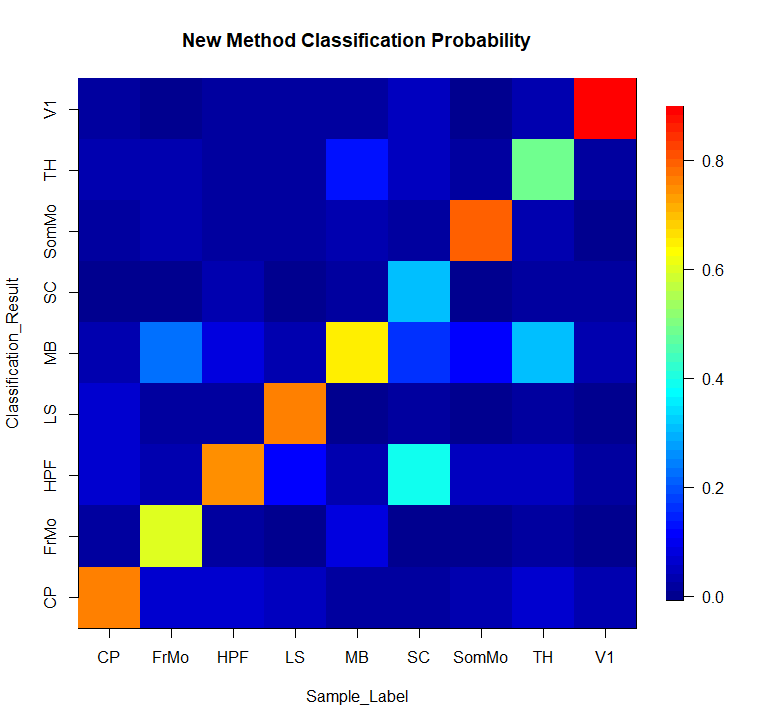
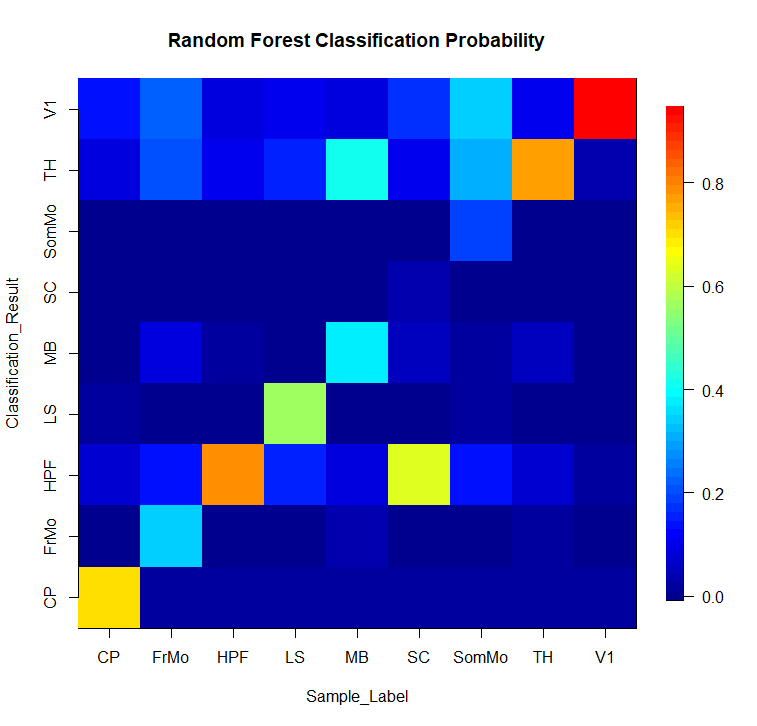
Figure 5: Heatmap of classification probabilities of the new method(left) and random forest (right). The x-axis are the true labels of the group and the y-axis are the labels of the groups the samples are classified into.

Various classification methods are applied to the dataset (PLSR is not implemented due to the large dataset size and the limit of server memory). We randomly split the dataset into training and testing sets with a 2:1 ratio and repeated the process 150 times. The resulting misclassification rates from each trial are presented in Figure 4. We see that the new method has the lowest misclassification rate, followed by the random forest approach. All other methods have much higher misclassification rates.

We next compare the new method and the random forest approach is more details (Figure 5). For the new method, we see that some of the neurons in the SC region are classified to HPF, which are two physically close brain regions (see Figure 3). These two regions are hard to distinguish and the random forest approach does even worse. In addition, the random forest approach does very badly for the SomMo region, resulting a overall worse performance compared to the new approach.

4 Explore quantities that play important roles

Given the good performance of the new approach in various settings in Section 3, we here try to explore the key factors that play important roles in the framework. In this section, we consider the following two-class setting (*):

$$X_{i}=\mathbf{A}(x_{i1},x_{i2},\dots,x_{id})^{\top},i=1,2,\dots,n;$$

$$\textit{where}\ \mathbf{A}\in\mathbb{R}^{d\times d},x_{ik}\stackrel{{\scriptstyle i.i.d.}}{{\sim}}F_{x},\textit{with}\ \mathbb{E}x_{11}=0,\mathbb{E}x_{11}^{4}<\infty;$$

$$Y_{j}=\mathbf{B}(y_{j1},y_{j2},\dots,y_{jd})^{\top}+\mu,j=1,2,\dots,m;$$

$$\textit{where}\ \mathbf{B}\in\mathbb{R}^{d\times d},y_{jk}\stackrel{{\scriptstyle i.i.d.}}{{\sim}}F_{y},\textit{with}\ \mathbb{E}y_{11}=0,\mathbb{E}y_{11}^{4}<\infty,$$

We use this setting (*) as the difference between the two classes can be easily controlled through $F_{x}$, $F_{y}$, $\mathbf{A}$ and $\mathbf{B}$. We aim to approximate the misclassification rate through quantities from $F_{x}$, $F_{y}$, $\mathbf{A}$ and $\mathbf{B}$. It is very difficult to handle Algorithm 1 directly as it involves ranks. We thus work on a similar algorithm but is much easier to handle.

4.1 Distance-based approach

To make the approach easier to analyze, we remove the steps of computing ranks. This distance-based approach is very similar to the rank-based version (Algorithm 1) and it also performs similarly under various simulation settings, but it is less robust than the rank-based version when there are outliers. Table 6 shows the results under the simulation settings in Section 3.1 (no outlier). We see that the two approaches showed similar performance under these settings.

Table 6: Two-class misclassification rate of the two approaches (no outliers)

	Scenario 1			Scenario 2			Scenario 3
$(\mu_{0},a)$	(0,1.1)	(6,0)	(6,1.1)	(0,1.1)	(6,0)	(6,1.1)	(0,1.1)	(6,0)	(6,1.1)
Rank	0.020	0.027	0.003	0.100	0.109	0.042	0.071	0.414	0.069
Dist	0.078	0.026	0.001	0.173	0.099	0.074	0.148	0.396	0.136

Algorithm 2 Distance-based classification

• Construct a distance matrix $D\in\mathbb{R}^{N\times N}$: $D[i,j]=\|Z_{i}-Z_{j}\|_{2}^{2}.$

• Construct a distance mean matrix $M^{(D)}\in\mathbb{R}^{N\times k}$:

  $$M^{(D)}[i,j]:=M^{(D)}_{j}(Z_{i})=\frac{1}{n_{j}-\mathbbm{1}\left\{g_{i}=j\right\}}\sum_{g_{l}=j,l\neq i}D[i,l].$$

• Construct a distance vector $D_{W}=(D_{W,1},D_{W,2},\dots D_{W,N})\in\mathbb{R}^{N}$, where $D_{W,i}=\|W-Z_{i}\|_{2}^{2}.$

• Construct a group distance vector $M^{(D)}_{W}=(M^{(D)}_{1}(W),M^{(D)}_{2}(W),\dots M^{(D)}_{k}(W))\in\mathbb{R}^{k}$, where

  $$M^{(D)}_{i}(W)=\frac{1}{n_{i}}\sum_{g_{l}=i}D_{W,l}.$$

• Use QDA to classify $M^{(D)}_{W}$:

  $$g^{(D)}(W)=\arg\max_{j}\left\{-\frac{1}{2}\log|\hat{\Sigma}^{(D)}_{j}|-\frac{1}{2}(M^{(D)}_{W}-\hat{\mu}_{j}^{(D)})^{\top}\hat{\Sigma}_{j}^{{(D)}^{-1}}(M^{(D)}_{W}-\hat{\mu}^{(D)}_{j})+\log\frac{n_{j}}{N}\right\},$$

  where $\hat{\mu}^{(D)}_{j}=\frac{1}{n_{j}}\sum_{i=1}^{N}M_{j}^{(D)}(Z_{i})\mathbbm{1}\left\{g_{i}=j\right\}$
  and $\hat{\Sigma}^{(D)}_{j}=\frac{1}{n_{j}-1}\sum_{i=1}^{N}\left(M_{j}^{(D)}(Z_{i})-\hat{\mu}^{(D)}_{j}\right)\left(M_{j}^{(D)}(Z_{i})-\hat{\mu}^{(D)}_{j}\right)^{\top}\mathbbm{1}\left\{g_{i}=j\right\}.$

On the other hand, if there are outliers in the data, the distance-based approach is much less robust. Considering the simulation setting scenario 1 (multi-normal distribution) in Section 3.1 but contaminated by outliers $X_{i}\sim(5(a-1)+1)\mathbf{A}(x_{i1},x_{i2},\dots,x_{id})^{\top}+5\mu$, $i=1,2,\dots n_{o}$, where $n_{o}$ is the number of outliers, and all other observations are simulated in the same way as before. Table 7 shows the misclassification rate of the two approaches. We see that with outliers, the distance-based has a much higher misclassification rate than the rank-based approach. Therefore, the rank-based approach is recommended to use in practice for its robustness. However, under the ideal scenario of no outliers, we could study the distance-based algorithm to approximate the rank-based version as the former is much easier to analyze.

Table 7: Two-class misclassification rate of the two approaches (with outliers)

$\mu_{0}$	$a$	$n_{o}$	Rank	Dist	$\mu_{0}$	$a$	$n_{o}$	Rank	Dist
0	1.1	1	0.0243	0.3081	0	1.1	3	0.0350	0.3246
6	1	1	0.0303	0.1275	6	1	3	0.0439	0.1410
6	1.1	1	0.0114	0.1269	6	1.1	3	0.0262	0.1510
0	1.1	5	0.0433	0.3352	0	1.1	7	0.0396	0.3378
6	1	5	0.0530	0.1694	6	1	7	0.0708	0.2287
6	1.1	5	0.0451	0.1747	6	1.1	7	0.0657	0.2265

4.2 Misclassification rate estimation through the distance-based approach

Define

$$D(X_{i})=\binom{D_{X}(X_{i})}{D_{Y}(X_{i})},\ D(Y_{i})=\binom{D_{X}(Y_{i})}{D_{Y}(Y_{i})},$$

where $D_{X}(X_{i})=\frac{1}{n-1}\sum_{k\neq i}\|X_{k}-X_{i}\|_{2}^{2}$, $D_{Y}(X_{i})=\frac{1}{m}\sum_{k=1}^{m}\|Y_{k}-X_{i}\|_{2}^{2}$, $D_{X}(Y_{i})=\frac{1}{n}\sum_{k=1}^{n}\|X_{k}-Y_{i}\|_{2}^{2}$, $D_{Y}(Y_{i})=\frac{1}{m-1}\sum_{k\neq i}\|Y_{k}-Y_{i}\|_{2}^{2}$. Under Setting (*), we can compute the expectation and covariance matrix of $D(X_{i})$ and $D(Y_{i})$ through the following theorems. The proofs are deferred to Appendix A.

Theorem 4.1.

Let $\left\{X_{i}\right\}_{i=1}^{n}$, $\left\{Y_{j}\right\}_{j=1}^{m}$ be generated from Setting (*), we have

$$\mathbb{E}(D(X_{i}))=\mu_{D_{X}}=f(\mathbf{A},\mathbf{B},\mu,F_{x},F_{y}),$$

$$\mathbb{E}(D(Y_{i}))=\mu_{D_{Y}}=f(\mathbf{B},\mathbf{A},-\mu,F_{y},F_{x}),$$

$$\textsf{Cov}(D(X_{i}))=\Sigma_{D_{X}}=g(n,m,\mathbf{A},\mathbf{B},\mu,F_{x},F_{y}),$$

$$\textsf{Cov}(D(Y_{i}))=\Sigma_{D_{Y}}=g(m,n,\mathbf{B},\mathbf{A},-\mu,F_{y},F_{x}).$$

where the $f(\cdot)\in\mathbb{R}^{2}$ and $g(\cdot)\in\mathbb{R}^{2\times 2}$:

$$f(\mathbf{A},\mathbf{B},\mu,F_{x},F_{y})=\left(\begin{matrix}2\|\mathbf{A}\|_{F}^{2}\mathbb{E}x_{11}^{2}\\ \|\mathbf{A}\|_{F}^{2}\mathbb{E}x_{11}^{2}+\|\mathbf{B}\|_{F}^{2}\mathbb{E}y_{11}^{2}+\|\mu\|_{2}^{2}\end{matrix}\right),$$

$$g(n,m,\mathbf{A},\mathbf{B},\mu,F_{x},F_{y})=-f(\mathbf{A},\mathbf{B},\mu,F_{x},F_{y})f(\mathbf{A},\mathbf{B},\mu,F_{x},F_{y})^{\top}$$

$$+\left(\begin{array}[]{cc}\frac{1}{n-1}\left\langle\left(\begin{array}[]{l}h_{1}(\mathbf{A},\mathbf{A},\mathbf{A},\mathbf{0},\mathbf{0},F_{x},F_{x},F_{x})\\ h_{2}(\mathbf{A},\mathbf{A},\mathbf{0},F_{x},F_{x})\end{array}\right),\left(\begin{array}[]{c}1\\ n-2\end{array}\right)\right\rangle&h_{1}(\mathbf{A},\mathbf{A},\mathbf{B},0,\mu,F_{x},F_{x},F_{y})\\ h_{1}(\mathbf{A},\mathbf{A},\mathbf{B},\mathbf{0},\mu,F_{x},F_{y})&\frac{1}{m}\left\langle\left(\begin{array}[]{l}h_{1}(\mathbf{A},\mathbf{B},\mathbf{B},\mu,\mu,F_{x},F_{y},F_{y})\\ h_{2}(\mathbf{A},\mathbf{B},\mu,F_{x},F_{y})\end{array}\right),\left(\begin{array}[]{c}1\\ m-1\end{array}\right)\right\rangle\end{array}\right),$$

and $h_{1}$ and $h_{2}$ defined in Lemma 4.2.

Lemma 4.2.

For $U=\mathbf{C}(u_{1},u_{2},\dots,u_{d})^{\top}$, $V=\mathbf{D}(v_{1},v_{2},\dots,v_{d})^{\top}$, where $u_{i}\stackrel{{\scriptstyle i.i.d.}}{{\sim}}F_{u}$, with $\mathbb{E}u=0$, $\mathbb{E}u^{4}<\infty$ and $v_{i}\stackrel{{\scriptstyle i.i.d.}}{{\sim}}F_{v}$, with $\mathbb{E}v=0$, $\mathbb{E}v^{4}<\infty$, $X_{i}=\mathbf{A}(x_{i1},x_{i2},\dots,x_{id})^{\top}$, $i=1,2,\dots,n$, $x_{ik}\stackrel{{\scriptstyle i.i.d.}}{{\sim}}F_{x}$, with $\mathbb{E}x_{11}=0$, $\mathbb{E}x_{11}^{4}<\infty$, $\mathbf{A},\mathbf{C},\mathbf{D}\in\mathbb{R}^{d\times d}$, we have

$$h_{1} (\mathbf{A},\mathbf{C},\mathbf{D},\mu_{u},\mu_{v},F_{x},F_{u},F_{v})=\|\mathbf{C}\|_{F}^{2}\mathbb{E}u_{1}^{2}\|\mathbf{D}\|_{F}^{2}\mathbb{E}v_{1}^{2}+\|\mathbf{D}\|_{F}^{2}\mathbb{E}v_{1}^{2}\|\mu_{u}\|_{2}^{2}$$

$$+\sum_{i=1}^{d}\sum_{j=1}^{d}(\sum_{k=1}^{d}a_{ik}^{2}a_{jk}^{2}\mathbb{E}x_{11}^{4}+\left(\sum_{k_{1}\neq k_{2}}a_{ik_{1}}^{2}a_{jk_{2}}^{2}+2\sum_{k_{1}\neq k_{2}}a_{ik_{1}}a_{ik_{2}}a_{jk_{1}}a_{jk_{2}}\right)(\mathbb{E}x_{11}^{2})^{2})$$

$$+(\|\mathbf{C}\|_{F}^{2}\mathbb{E}u_{1}^{2}+\|\mathbf{D}\|_{F}^{2}\mathbb{E}v_{1}^{2})\|\mathbf{A}\|_{F}^{2}\mathbb{E}x_{11}^{2}+(\|\mu_{u}\|_{2}^{2}+\|\mu_{v}\|_{2}^{2})\|\mathbf{A}\|_{F}^{2}\mathbb{E}x_{11}^{2}+\|\mu_{u}\|_{2}^{2}\|\mu_{v}\|_{2}^{2}$$

$$-2\sum_{i=1}^{d}\sum_{j=1}^{d}(\sum_{k=1}^{d}a_{ik}^{2}a_{jk}(\mu_{uk}+\mu_{vk}))\mathbb{E}x_{11}^{3}+\|\mathbf{C}\|_{F}^{2}\mathbb{E}u_{1}^{2}\|\mu_{v}\|_{2}^{2},$$

$$h_{2} (\mathbf{A},\mathbf{C},\mu_{u},F_{x},F_{u})=2\|\mu_{u}\|_{2}^{2}(\|\mathbf{C}\|_{F}^{2}\mathbb{E}u_{1}^{2}+\|\mathbf{A}\|_{F}^{2}\mathbb{E}x_{11}^{2})+4\|\mu_{u}\mathbf{C}\|_{F}^{2}\mathbb{E}u_{1}^{2}$$

$$+\sum_{i=1}^{d}\sum_{j=1}^{d}(\sum_{k=1}^{d}c_{ik}^{2}c_{jk}^{2}\mathbb{E}u_{1}^{4}+\left(\sum_{k_{1}\neq k_{2}}c_{ik_{1}}^{2}c_{jk_{2}}^{2}+2\sum_{k_{1}\neq k_{2}}c_{ik_{1}}c_{ik_{2}}c_{jk_{1}}c_{jk_{2}}\right)(\mathbb{E}u_{1}^{2})^{2})$$

$$+\sum_{i=1}^{d}\sum_{j=1}^{d}(\sum_{k=1}^{d}a_{ik}^{2}a_{jk}^{2}\mathbb{E}x_{11}^{4}+\left(\sum_{k_{1}\neq k_{2}}a_{ik_{1}}^{2}a_{jk_{2}}^{2}+2\sum_{k_{1}\neq k_{2}}a_{ik_{1}}a_{ik_{2}}a_{jk_{1}}a_{jk_{2}}\right)(\mathbb{E}x_{11}^{2})^{2})$$

$$+4\sum_{i=1}^{d}\sum_{j=1}^{d}(\sum_{k=1}^{d}c_{ik}^{2}c_{jk}\mu_{k})\mathbb{E}u_{1}^{3}-4\sum_{i=1}^{d}\sum_{j=1}^{d}(\sum_{k=1}^{d}a_{ik}^{2}a_{jk}\mu_{k})\mathbb{E}x_{11}^{3}+4\|\mu_{u}\mathbf{A}\|_{F}^{2}\mathbb{E}x_{11}^{2}$$

$$+2\|\mathbf{C}\|_{F}^{2}\mathbb{E}u_{1}^{2}\|\mathbf{A}\|_{F}^{2}\mathbb{E}x_{11}^{2}+\|\mu_{u}\|_{2}^{4}+4\|\mathbf{A}^{\top}\mathbf{C}\|_{F}^{2}\mathbb{E}u_{1}^{2}\mathbb{E}x_{11}^{2}.$$

For a testing sample, suppose $W_{x}\sim F_{X}$ (the distribution of $X_{i}$’s) and $W_{y}\sim F_{Y}$ (the distribution of $Y_{j}$’s), we can also obtain the expectation and covariance matrix of $D(W_{x})$ and $D(W_{y})$ in a similar way, where $D(W)=\binom{D_{X}(W)}{D_{Y}(W)}$ with $D_{X}(W)=\frac{1}{n}\sum_{k=1}^{n}\|X_{k}-W\|_{2}^{2}$ and $D_{Y}(W)=\frac{1}{m}\sum_{k=1}^{m}\|Y_{k}-W\|_{2}^{2}$.

Theorem 4.3.

Under Setting (*), the the expectation and covariance matrix of $D(W_{x})$ and $D(W_{y})$ are given by:

$$\mathbb{E}(D(W_{x}))=\mu_{D_{W_{x}}} =f(\mathbf{A},\mathbf{B},\mu,F_{x},F_{y}),$$

$$\textsf{Cov}(D(W_{x}))=\Sigma_{D_{W_{x}}} =g(n+1,m,\mathbf{A},\mathbf{B},\mu,F_{x},F_{y}),$$

$$\mathbb{E}(D(W_{y}))=\mu_{D_{W_{y}}} =f(\mathbf{B},\mathbf{A},-\mu,F_{y},F_{x}),$$

$$\textsf{Cov}(D(W_{y}))=\Sigma_{D_{W_{y}}} =g(m+1,n,\mathbf{B},\mathbf{A},-\mu,F_{y},F_{x}).$$

If we further add constraints on $\mathbf{A}$ and $\mathbf{B}$, we can obtain the asymptotic distribution of the distance mean vector $D(\cdot)$.

Theorem 4.4.

In Setting (*), let $s=\lfloor d^{\frac{1}{5}}\rfloor$, $t=\lfloor d/t\rfloor$, $r=d-st$,

$$\mathbf{A}=\left(\begin{matrix}a_{1}^{T}\\ a_{2}^{T}\\ \vdots\\ a_{d}^{T}\end{matrix}\right),\ \mathbf{B}=\left(\begin{matrix}b_{1}^{T}\\ b_{2}^{T}\\ \vdots\\ b_{d}^{T}\end{matrix}\right),\ R_{i}=\sum_{k=(i-1)s+1}^{is-m_{0}}\begin{pmatrix}\frac{1}{n-1}\sum_{j\neq i}^{n}(a_{k}^{T}X_{j}-a_{k}^{T}X_{1})^{2}\\ \frac{1}{m}\sum_{j=1}^{m}(b_{k}^{T}Y_{j}-a_{k}^{T}X_{1}+\mu_{k})^{2}\end{pmatrix},$$

and $\Sigma_{t}=\textsf{Cov}(\sum_{i=1}^{t}R_{i})$. If $\mathbf{A}$ and $\mathbf{B}$ are band matrix, where $a_{ij}=0,\forall\ |i-j|\geq m_{0}$; $b_{ij}=0,\forall\ |i-j|\geq m_{0}$, with $m_{0}$ is a fixed number, $\max\{|\mu_{i}|\}<\mu_{0}$, $\max\left\{|a_{ij}|,|b_{ij}|\right\}<c_{0}$, with $c_{0}$ and $\mu_{0}$ fixed numbers, and $\lim_{t\to\infty}\sum_{i=1}^{t}\mathbb{E}\left(\|\Sigma_{t}^{-\frac{1}{2}}R_{i}\|_{2}^{3}\right)\to 0$, then $\frac{1}{\sqrt{d}}(D(X_{i})-\mu_{D_{X}})$ converges to a normal distribution as $d\to\infty$.

Remark 2.

The condition $\lim_{t\to\infty}\sum_{i=1}^{t}\mathbb{E}\left(\|\Sigma_{t}^{-\frac{1}{2}}R_{i}\|_{2}^{3}\right)\to 0$ in Theorem 4.4 could be hard to comprehend. Here, we provide a simple case that the condition is satisfied when all $\mu_{i}$’s are the same: non-zero elements in $a_{i}^{T}$’s are the same and non-zero elements in $b_{i}^{T}$’s are the same, i.e. $\exists\ \alpha=(\alpha_{1},\alpha_{2},\dots,\alpha_{2m_{0}-1})$ and $\beta=(\beta_{1},\beta_{2},\dots,\beta_{2m_{0}-1})$, $\mathbf{A}_{ij}=\alpha_{m_{0}+j-i}$, $\mathbf{B}_{ij}=\beta_{m_{0}+j-i}$, $\forall\ |i-j|<m_{0}$.

The proofs of Theorem 4.4 and Remark 2 are provided in Appendix B.

Remark 3.

We can also prove the asymptotic normality of $\frac{1}{\sqrt{d}}(D(Y_{j})-\mu_{D(Y)})$, $\frac{1}{\sqrt{d}}(D(W_{x_{i}})-\mu_{D(W_{x})})$ and $\frac{1}{\sqrt{d}}(D(W_{y_{j}})-\mu_{D(W_{y})})$ by changing the conditions in 4.4. By substituting $\mathbf{A}$ with $\mathbf{B}$, $\mathbf{B}$ with $\mathbf{A}$, $\mu$ with $-\mu$, $n$ with $m$ and $m$ with $n$, we can obtain the conditions for $\frac{1}{\sqrt{d}}(D(Y_{j})-\mu_{D(Y)})$; by substituting $n$ with $n+1$, we can obtain the conditions for $\frac{1}{\sqrt{d}}(D(W_{x_{i}})-\mu_{D(W_{x})})$; by substituting $\mathbf{A}$ with $\mathbf{B}$, $\mathbf{B}$ with $\mathbf{A}$, $\mu$ with $-\mu$, $n$ with $m+1$ and $m$ with $n$, we can obtain the conditions for $\frac{1}{\sqrt{d}}(D(W_{y_{j}})-\mu_{D(W_{y})})$.

By sampling $D_{W}$ from $0.5N(\mu_{D_{W_{x}}},\Sigma_{D_{W_{x}}})+0.5N(\mu_{D_{W_{y}}},\Sigma_{D_{W_{y}}})$ and applying the decision rule to each $D_{W}$ with

$$\delta_{X}=-\frac{1}{2}log|\Sigma_{D_{X}}|-\frac{1}{2}(D_{W}-\mu_{D_{X}})^{\top}\Sigma_{D_{X}}^{-1}(D_{W}-\mu_{D_{X}}),$$

$$\delta_{Y}=-\frac{1}{2}log|\Sigma_{D_{Y}}|-\frac{1}{2}(D_{W}-\mu_{D_{Y}})^{\top}\Sigma_{D_{Y}}^{-1}(D_{W}-\mu_{D_{Y}}),$$

we can estimate the misclassification rate by simulating the last step.

We now test our estimation through numerical simulations. Under setting (*), we set $n=50$, $m=50$, $d=2000$, $\mathbf{B}=a\mathbf{A}$, $\mathbf{A}\mathbf{A}^{\top}=\Sigma$, with $\Sigma_{r,c}=0.1^{|r-c|}$, where $\mu=\mu_{0}\frac{\mu^{\prime}}{\|\mu^{\prime}\|}$, $\mu^{\prime}$ is a random vector generated from $N_{d}(0,\mathbf{I}_{d})$. The testing samples $W_{x_{1}},W_{x_{2}},\dots W_{x_{50}}\stackrel{{\scriptstyle\text{ i.i.d }}}{{\sim}}F_{X}$ and $W_{y_{1}},W_{y_{2}},\dots W_{y_{50}}\stackrel{{\scriptstyle\text{ i.i.d }}}{{\sim}}F_{Y}$ . We consider the following scenarios:

• Scenario 10: $F_{x}=N(0,1)$, $F_{y}=N(0,1)$; fix $a=1$ and change $\mu_{0}$;

• Scenario 11: $F_{x}=N(0,1)$, $F_{y}=N(0,1)$; fix $\mu=0$ and change $a$.

• Scenario 12: $F_{x}=t_{10}$, $F_{y}=t_{10}$; fix $a=1$ and change $\mu_{0}$;

• Scenario 13: $F_{x}=t_{10}$, $F_{y}=t_{10}$; fix $\mu=0$ and change $a$.

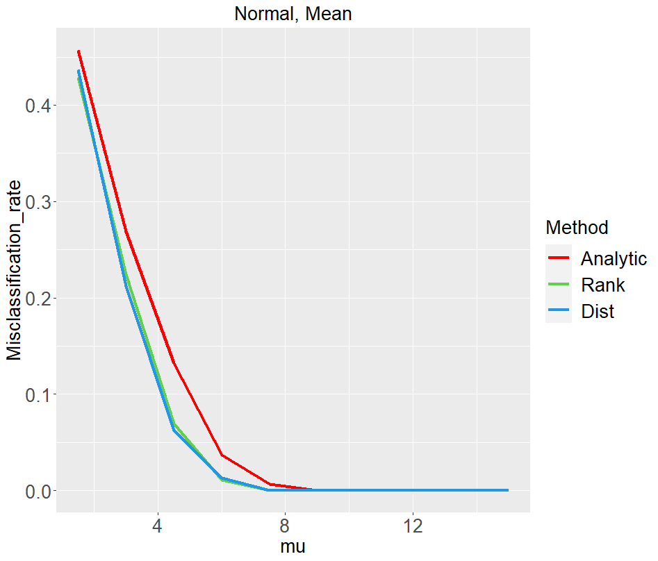
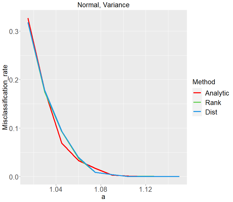
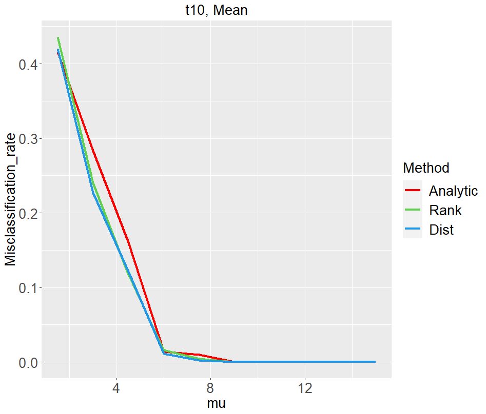
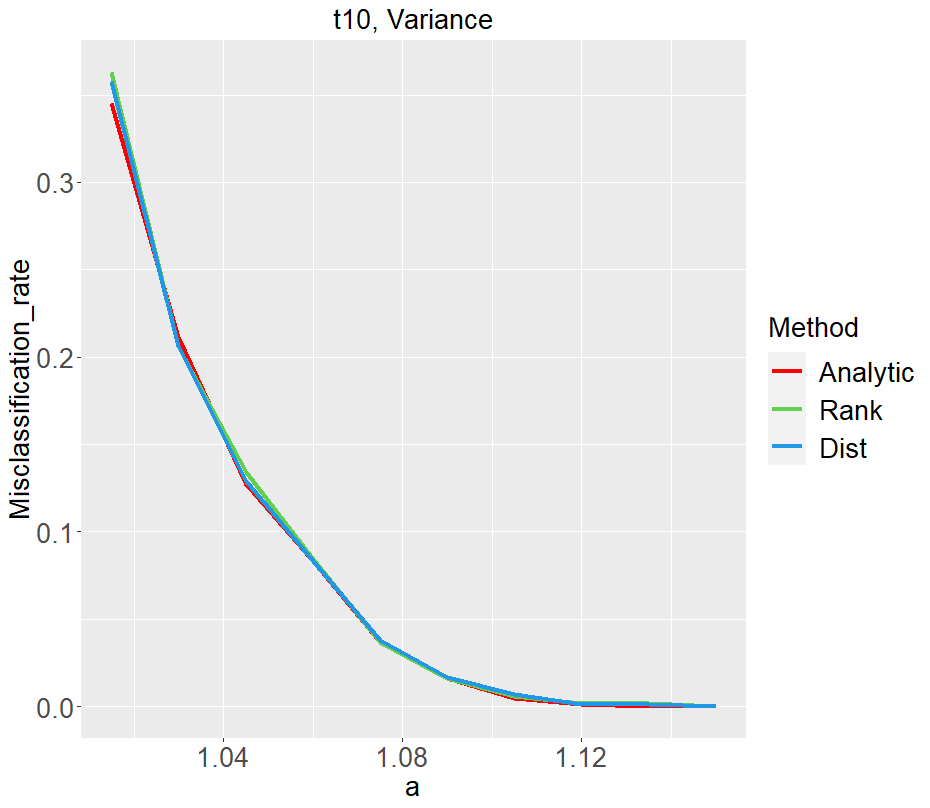
Figure 6: Analytic (red) and simulated (rank-based approach: green; distance-based approach: blue) misclassification rates for scenario 10 (upper-left panel), scenario 11 (upper-right panel), scenario 12 (bottom-left panel), scenario 13 (bottom-right panel).

Figure 6 shows the analytic misclassification rate (through the formulas in this section) and the simulated misclassification rate (through 50 simulation runs on Algorithm 1 and 2) in these scenarios. We see that the analytic misclassification rates are quite close to the simulated ones. Thus, the formulas used in estimating the misclassification rate are likely to contain the key quantities from the distributions that play important roles in Algorithm 1. By examining the formulas, we see that the first and second moments of $F_{x}$ and $F_{y}$ play extremely important roles (through the $f(\cdot)$ function), which is likely the reason that the new method works well for mean and/or variance differences, and the higher moments of $F_{x}$ and $F_{y}$ (the third and fourth moments) play some roles (through the $g(\cdot)$ function).

It should be noted that, the vectors used in the decision rule in the last step of both the rank-based and distance-based versions of the new method are not independent. Specifically, in the distance-based version, $M^{(D)}_{W}$ is dependent on $M^{(D)}_{j}(Z_{i})$’s (similarly for the rank-based version with $M_{W}$). We also study an independent version of the distance-based approach in Appendix C. We find that this dependency does not affect the misclassification rate of the method much.

5 Conclusion

We propose a novel framework for high-dimensional classification that leverages a common pattern in high-dimensional data and exhibits strong performance across various simulation settings and real data analyses. Furthermore, we provide a basic theoretical analysis of the method to gain some understandings on how the method works.

The approach proposed in this paper utilizes the $l_{2}$ distance as the dissimilarity measure between samples. However, it is not limited to this measure and can be extended to other types of dissimilarity measures as well. It would be interesting to explore the performance of the new method using different distances and we will explore this in future work.

Appendix A Proof of Theorem 4.1, Lemma 4.2 and Theorem 4.3

Under Setting (*), let $\boldsymbol{x_{i}}=(x_{i1},x_{i2},\dots,x_{id})^{\top}$, we have

$$\mathbb{E}\|X_{k}-X_{i}\|_{2}^{2} =\mathbb{E}\|\mathbf{A}(\boldsymbol{x_{k}}-\boldsymbol{x_{i}})\|_{2}^{2}=\mathbb{E}\boldsymbol{x_{i}}^{\top}\mathbf{A}^{\top}\mathbf{A}\boldsymbol{x_{i}}-2\mathbb{E}\boldsymbol{x_{k}}^{\top}\mathbf{A}^{\top}\mathbf{A}\boldsymbol{x_{i}}+\mathbb{E}\boldsymbol{x_{i}}^{\top}\mathbf{A}^{\top}\mathbf{A}\boldsymbol{x_{i}}$$

$$=2tr(\mathbf{A}^{\top}\mathbf{A})\mathbb{E}x_{11}^{2}=2\|\mathbf{A}\|_{F}^{2}\mathbb{E}x_{11}^{2},$$

$$\mathbb{E}\|Y_{k}-X_{i}\|_{2}^{2} =\mathbb{E}\|\mathbf{B}\boldsymbol{y_{k}}-\mathbf{A}\boldsymbol{x_{i}}+\mu\|_{2}^{2}=\mathbb{E}\boldsymbol{y_{k}}^{\top}\mathbf{B}^{\top}\mathbf{B}\boldsymbol{y_{k}}+\mathbb{E}\boldsymbol{x_{i}}^{\top}\mathbf{A}^{\top}\mathbf{A}\boldsymbol{x_{i}}$$

$$\quad-2\mathbb{E}\boldsymbol{y_{k}}^{\top}\mathbf{B}^{\top}\mathbf{A}\boldsymbol{x_{i}}+2\mathbb{E}<\mathbf{B}\boldsymbol{y_{k}}-\mathbf{A}\boldsymbol{x_{i}},\mu>+\|\mu\|_{2}^{2}$$

$$=\|\mathbf{A}\|_{F}^{2}\mathbb{E}x_{11}^{2}+\|\mathbf{B}\|_{F}^{2}\mathbb{E}y_{11}^{2}+\|\mu\|_{2}^{2}.$$

Then $\mathbb{E}(D(X_{i}))$ follows straightforwardly by the linearity of expectation. Also, $\mathbb{E}(D(Y_{i}))$, $\mathbb{E}(D(W_{x}))$ and $\mathbb{E}(D(W_{y}))$ can be obtained similarly.

To get the covariance matrix of $D(X_{i})$, we need to compute $\textsf{Var}(D_{X}(X_{i}))$, $\textsf{Var}(D_{X}(X_{i}))$ and $\textsf{Cov}(D_{X}(X_{i}),D_{Y}(X_{i}))$ respectively.

$$\textsf{Var}(D_{X}(X_{i})) =\mathbb{E}\left(\frac{1}{n-1}\sum_{k\neq i}\|X_{k}-X_{i}\|_{2}^{2}\right)^{2}-\mathbb{E}^{2}(D_{X}(X_{i}))$$

$$=\frac{1}{(n-1)^{2}}\mathbb{E}\left(\sum_{k_{1}\neq k_{2}}(\|X_{k_{1}}-X_{i}\|_{2}^{2}\cdot\|X_{k_{2}}-X_{i}\|_{2}^{2})+\sum_{k\neq i}\|X_{k}-X_{i}\|_{2}^{4}\right)-\mathbb{E}^{2}(D_{X}(X_{i}))$$

$$=\frac{n-2}{n-1}\mathbb{E}(\|X_{k_{1}}-X_{i}\|_{2}^{2}\cdot\|X_{k_{2}}-X_{i}\|_{2}^{2})+\frac{1}{n-1}\mathbb{E}\|X_{k}-X_{i}\|_{2}^{4}-\mathbb{E}^{2}(D_{X}(X_{i}))$$

$$\textsf{Var}(D_{Y}(X_{i})) =\mathbb{E}\left(\frac{1}{m}\sum_{k=1}^{m}\|Y_{k}-X_{i}\|_{2}^{2}\right)^{2}-\mathbb{E}^{2}(D_{Y}(X_{i}))$$

$$=\frac{1}{m^{2}}\mathbb{E}\left(\sum_{k_{1}\neq k_{2}}(\|Y_{k_{1}}-X_{i}\|_{2}^{2}\cdot\|Y_{k_{2}}-X_{i}\|_{2}^{2})+\sum_{k=1}^{m}\|Y_{k}-X_{i}\|_{2}^{4}\right)-\mathbb{E}^{2}(D_{Y}(X_{i}))$$

$$=\frac{1}{m}\mathbb{E}\|Y_{k}-X_{i}\|_{2}^{4}+\frac{m-1}{m}\mathbb{E}(\|Y_{k_{1}}-X_{i}\|_{2}^{2}\cdot\|Y_{k_{2}}-X_{i}\|_{2}^{2})-\mathbb{E}^{2}(D_{Y}(X_{i}))$$

$$\textsf{Cov}(D_{X}(X_{i}),D_{Y}(X_{i})) =\mathbb{E}\left(\left(\frac{1}{n-1}\sum_{k\neq i}\|X_{k}-X_{i}\|_{2}^{2}\right)\left(\frac{1}{m}\sum_{k=1}^{m}\|Y_{k}-X_{i}\|_{2}^{2}\right)\right)-\mathbb{E}(D_{X}(X_{i}))\cdot\mathbb{E}(D_{Y}(X_{i}))$$

$$=\mathbb{E}(\|X_{k_{1}}-X_{i}\|_{2}^{2}\cdot\|Y_{k_{2}}-X_{i}\|_{2}^{2})-\mathbb{E}(D_{X}(X_{i}))\cdot\mathbb{E}(D_{Y}(X_{i}))$$

We will compute the following quantities first:

Let $a_{ij}$ denote the $(i,j)$ element in $\mathbf{A}$. For $s\in\mathbb{R}^{d}$, we have

$$\mathbb{E}\|\mathbf{A}s\|_{2}^{4} =\sum_{i=1}^{d}\sum_{j=1}^{d}\mathbb{E}\left(\left(\sum_{t=1}^{d}a_{it}s_{t}\right)^{2}\left(\sum_{t=1}^{d}a_{jt}s_{t}\right)^{2}\right)$$ (1)

$$=\sum_{i=1}^{d}\sum_{j=1}^{d}\mathbb{E}\left(\left(\sum_{t=1}^{d}a_{it}^{2}s_{t}^{2}+\sum_{t\neq l}a_{it}a_{il}s_{t}s_{l}\right)\left(\sum_{t=1}^{d}a_{jt}^{2}s_{t}^{2}+\sum_{t\neq l}a_{jt}a_{jl}s_{t}s_{l}\right)\right).$$

Then, for $s=(x_{i1},x_{i2},\dots,x_{id})^{\top}$ and $x_{ik}\stackrel{{\scriptstyle i.i.d.}}{{\sim}}F_{x}$ with $\mathbb{E}x_{11}=0$, we have

$$\mathbb{E}\|\mathbf{A}s\|_{2}^{4} =\sum_{i=1}^{d}\sum_{j=1}^{d}\mathbb{E}\left(\sum_{t=1}^{d}a_{it}^{2}s_{t}^{2}\sum_{t=1}^{d}a_{jt}^{2}s_{t}^{2}+\sum_{{t_{1}}\neq{l_{1}}}a_{i{t_{1}}}a_{i{l_{1}}}s_{t_{1}}s_{l_{1}}\sum_{{t_{2}}\neq{l_{2}}}a_{j{t_{2}}}a_{j{l_{2}}}s_{t_{2}}s_{l_{2}}\right)$$ (2)

$$=\sum_{i=1}^{d}\sum_{j=1}^{d}\left(\sum_{k=1}^{d}a_{ik}^{2}a_{jk}^{2}\mathbb{E}x_{11}^{4}+\left(\sum_{k_{1}\neq k_{2}}a_{ik_{1}}^{2}a_{jk_{2}}^{2}+2\sum_{k_{1}\neq k_{2}}a_{ik_{1}}a_{ik_{2}}a_{jk_{1}}a_{jk_{2}}\right)(\mathbb{E}x_{11}^{2})^{2}\right).$$

$$\mathbb{E}\mu^{T}\mathbf{A}s\|\mathbf{A}s\|_{2}^{2} =\sum_{i=1}^{d}\sum_{j=1}^{d}\mathbb{E}(\sum_{t=1}^{d}\mu_{t}a_{it}s_{t})(\sum_{t=1}^{d}a_{jt}s_{t})^{2}=\sum_{i=1}^{d}\sum_{j=1}^{d}(\sum_{k=1}^{d}a_{ik}^{2}a_{jk}\mu_{k})\mathbb{E}x_{11}^{3}$$

For $U=\mathbf{C}(u_{1},u_{2},\dots,u_{d})^{\top},i=1,2,\dots,n$, $V=\mathbf{D}(v_{1},v_{2},\dots,v_{d})^{\top}$:

$$\mathbb{E}(\|U+\mu_{u}-X_{i}\|_{2}^{2}\cdot\|V+\mu_{v}-X_{i}\|_{2}^{2})=\mathbb{E}(\mathbb{E}(\|U+\mu_{u}-X_{i}\|_{2}^{2}\cdot\|V+\mu_{v}-X_{i}\|_{2}^{2})|X_{i})$$ (3)

$$=\mathbb{E}_{s}(\|\mathbf{C}\|_{F}^{2}\mathbb{E}u_{1}^{2}+\|\mathbf{A}s\|_{2}^{2}-2\mu_{u}^{\top}\mathbf{A}s+\|\mu_{u}\|_{2}^{2})(\|\mathbf{D}\|_{F}^{2}\mathbb{E}v_{1}^{2}+\|\mathbf{A}s\|_{2}^{2}-2\mu_{v}^{\top}\mathbf{A}s+\|\mu_{v}\|_{2}^{2})$$

$$=\|\mathbf{C}\|_{F}^{2}\mathbb{E}u_{1}^{2}\|\mathbf{D}\|_{F}^{2}\mathbb{E}v_{1}^{2}+(\|\mathbf{C}\|_{F}^{2}\mathbb{E}u_{1}^{2}+\|\mathbf{D}\|_{F}^{2}\mathbb{E}v_{1}^{2})\|\mathbf{A}\|_{F}^{2}\mathbb{E}x_{11}^{2}+\|\mathbf{C}\|_{F}^{2}\mathbb{E}u_{1}^{2}\|\mu_{v}\|_{2}^{2}$$

$$\quad+\|\mathbf{D}\|_{F}^{2}\mathbb{E}v_{1}^{2}\|\mu_{u}\|_{2}^{2}+\mathbb{E}_{s}\|\mathbf{A}s\|_{2}^{4}-2\mathbb{E}_{s}(\mu_{u}^{\top}+\mu_{v}^{\top})\mathbf{A}s\|\mathbf{A}s\|_{2}^{2}$$

$$\quad+(\|\mu_{u}\|_{2}^{2}+\|\mu_{v}\|_{2}^{2})\|\mathbf{A}\|_{F}^{2}\mathbb{E}x_{11}^{2}+\|\mu_{u}\|_{2}^{2}\|\mu_{v}\|_{2}^{2}$$

By substituting $\mathbf{C}$, $\mathbf{D}$, $\mu_{u}$ , $\mu_{v}$ and the moments of $u_{1}$ and $v_{1}$ with proper quantities, we can get $\mathbb{E}(\|X_{k_{1}}-X_{i}\|_{2}^{2}\cdot\|X_{k_{2}}-X_{i}\|_{2}^{2})$ , $\mathbb{E}(\|X_{k_{1}}-X_{i}\|_{2}^{2}\cdot\|Y_{k_{2}}-X_{i}\|_{2}^{2})$ and $\mathbb{E}(\|Y_{k_{1}}-X_{i}\|_{2}^{2}\cdot\|Y_{k_{2}}-X_{i}\|_{2}^{2})$, respectively.

$$\mathbb{E}\|U+\mu_{u}-X_{i}\|_{2}^{4}=\mathbb{E}(\|\mu_{u}\|_{2}^{2}+\|\mathbf{C}u\|_{2}^{2}+\|\mathbf{A}s\|_{2}^{2}+2\mu_{u}^{\top}(\mathbf{C}u-\mathbf{A}s)-2s^{\top}\mathbf{A}^{\top}\mathbf{C}u)^{2}$$ (4)

$$=\mathbb{E}\|\mathbf{C}u\|_{2}^{4}+\mathbb{E}\|\mathbf{A}s\|_{2}^{4}+\|\mu_{u}\|_{2}^{4}+2\|\mu_{u}\|_{2}^{2}(\|\mathbf{C}\|_{F}^{2}\mathbb{E}u_{1}^{2}+\|\mathbf{A}\|_{F}^{2}\mathbb{E}x_{11}^{2})$$

$$\quad+2\|\mathbf{C}\|_{F}^{2}\mathbb{E}u_{1}^{2}\|\mathbf{A}\|_{F}^{2}\mathbb{E}x_{11}^{2}+4\mathbb{E}\mu_{u}^{T}\mathbf{C}u\|\mathbf{C}u\|_{2}^{2}-4\mathbb{E}\mu^{T}\mathbf{A}s\|\mathbf{A}s\|_{2}^{2}$$

$$\quad+4\|\mu_{u}\mathbf{C}\|_{F}^{2}\mathbb{E}u_{1}^{2}+4\|\mu_{u}\mathbf{A}\|_{F}^{2}\mathbb{E}x_{11}^{2}+4\|\mathbf{A}^{\top}\mathbf{C}\|_{F}^{2}\mathbb{E}u_{1}^{2}\mathbb{E}x_{11}^{2}$$

By substituting $\mathbf{C}$ and $\mathbf{D}$ with $\mathbf{A}$, $\mu_{u}$ and $\mu_{v}$ with $\boldsymbol{0}$, $F_{u}$ and $F_{v}$ with $F_{x}$ in (1) to (4), we have

$$\textsf{Var}(D_{X}(X_{i}))$$ (5)

$$=\frac{n-2}{n-1}\mathbb{E}(\|X_{k_{1}}-X_{i}\|_{2}^{2}\cdot\|X_{k_{2}}-X_{i}\|_{2}^{2})+\frac{1}{n-1}\mathbb{E}\|X_{k}-X_{i}\|_{2}^{4}-\mathbb{E}^{2}(D_{X}(X_{i}))$$

$$=\frac{n-2}{n-1}\biggl{(}\|\mathbf{A}\|_{F}^{4}\mathbb{E}x_{11}^{4}+2\|\mathbf{A}\|_{F}^{4}(\mathbb{E}x_{11}^{2})^{2}$$

$$\quad\quad\quad\quad+\sum_{i=1}^{d}\sum_{j=1}^{d}(\sum_{k=1}^{d}a_{ik}^{2}a_{jk}^{2}\mathbb{E}x_{11}^{4}+(\sum_{k_{1}\neq k_{2}}a_{ik_{1}}^{2}a_{jk_{2}}^{2}+2\sum_{k_{1}\neq k_{2}}a_{ik_{1}}a_{ik_{2}}a_{jk_{1}}a_{jk_{2}})(\mathbb{E}x_{11}^{2})^{2})\biggr{)}$$

$$\quad+\frac{1}{n-1}\left(2\mathbb{E}\|\mathbf{A}s\|_{2}^{4}+2\|\mathbf{A}\|_{F}^{4}(\mathbb{E}x_{11}^{2})^{2}+4\|\mathbf{A}^{\top}\mathbf{A}\|_{F}^{2}(\mathbb{E}x_{11}^{2})^{2}\right)-4\|\mathbf{A}\|_{F}^{4}(\mathbb{E}x_{11}^{2})^{2}$$

$$=\frac{n-2}{n-1}\|\mathbf{A}\|_{F}^{4}\mathbb{E}x_{11}^{4}-2\|\mathbf{A}\|_{F}^{4}(\mathbb{E}x_{11}^{2})^{2}+\frac{4}{n-1}\|\mathbf{A}^{\top}\mathbf{A}\|_{F}^{2}(\mathbb{E}x_{11}^{2})^{2})$$

$$\quad+\frac{n}{n-1}\sum_{i=1}^{d}\sum_{j=1}^{d}\left(\sum_{k=1}^{d}a_{ik}^{2}a_{jk}^{2}\mathbb{E}x_{11}^{4}+(\sum_{k_{1}\neq k_{2}}a_{ik_{1}}^{2}a_{jk_{2}}^{2}+2\sum_{k_{1}\neq k_{2}}a_{ik_{1}}a_{ik_{2}}a_{jk_{1}}a_{jk_{2}})(\mathbb{E}x_{11}^{2})^{2})\right).$$

By substituting $\mathbf{C}$ with $\mathbf{A}$, $\mathbf{D}$ with $\mathbf{B}$, $\mu_{u}$ with $\boldsymbol{0}$ and $\mu_{v}$ with $\mu$, $F_{u}$ with $F_{x}$ and $F_{v}$ with $F_{y}$ in (1) to (4), we have

$$\textsf{Cov}(D_{X}(X_{i}),D_{Y}(X_{i}))$$ (6)

$$=\mathbb{E}(\|X_{k_{1}}-X_{i}\|_{2}^{2}\cdot\|Y_{k_{2}}-X_{i}\|_{2}^{2})-\mathbb{E}(D_{X}(X_{i}))\cdot\mathbb{E}(D_{Y}(X_{i}))$$

$$=\|\mathbf{A}\|_{F}^{2}\|\mathbf{B}\|_{F}^{2}\mathbb{E}x_{11}^{2}\mathbb{E}y_{11}^{2}+(\|\mathbf{A}\|_{F}^{2}\mathbb{E}x_{11}^{2}+\|\mathbf{B}\|_{F}^{2}\mathbb{E}y_{11}^{2})\|\mathbf{A}\|_{F}^{2}\mathbb{E}x_{11}^{2}$$

$$\quad+\|\mathbf{A}\|_{F}^{2}\mathbb{E}x_{11}^{2}\|\mu\|_{2}^{2}+\mathbb{E}_{s}\|\mathbf{A}s\|_{2}^{4}-2\mathbb{E}_{s}\mu^{\top}\mathbf{A}s\|\mathbf{A}s\|_{2}^{2}$$

$$\quad+\|\mu\|_{2}^{2}\|\mathbf{A}\|_{F}^{2}\mathbb{E}x_{11}^{2}-2\|\mathbf{A}\|_{F}^{2}\mathbb{E}x_{11}^{2}\cdot(\|\mathbf{A}\|_{F}^{2}\mathbb{E}x_{11}^{2}+\|\mathbf{B}\|_{F}^{2}\mathbb{E}y_{11}^{2}+\|\mu\|_{2}^{2})$$

$$=\mathbb{E}_{s}\|\mathbf{A}s\|_{2}^{4}-2\mathbb{E}_{s}\mu^{\top}\mathbf{A}s\|\mathbf{A}s\|_{2}^{2}-\|\mathbf{A}\|_{F}^{4}(\mathbb{E}x_{11}^{2})^{2}$$

$$=\sum_{i=1}^{d}\sum_{j=1}^{d}\left(\sum_{k=1}^{d}a_{ik}^{2}a_{jk}^{2}\mathbb{E}x_{11}^{4}+\left(\sum_{k_{1}\neq k_{2}}a_{ik_{1}}^{2}a_{jk_{2}}^{2}+2\sum_{k_{1}\neq k_{2}}a_{ik_{1}}a_{ik_{2}}a_{jk_{1}}a_{jk_{2}}\right)(\mathbb{E}x_{11}^{2})^{2}\right)$$

$$\quad-\sum_{i=1}^{d}\sum_{j=1}^{d}(\sum_{k=1}^{d}a_{ik}^{2}a_{jk}\mu_{k})\mathbb{E}x_{11}^{3}-\|\mathbf{A}\|_{F}^{4}(\mathbb{E}x_{11}^{2})^{2}$$

By substituting $\mathbf{C}$ and $\mathbf{D}$ with $\mathbf{B}$, $\mu_{u}$ and $\mu_{v}$ with $\mu$, $F_{u}$ and $F_{v}$ with $F_{y}$ in (1) to (4), we have:

$$\textsf{Var}(D_{Y}(X_{i}))$$ (7)

$$=\frac{1}{m}\mathbb{E}\|Y_{k}-X_{i}\|_{2}^{4}+\frac{m-1}{m}\mathbb{E}(\|Y_{k_{1}}-X_{i}\|_{2}^{2}\cdot\|Y_{k_{2}}-X_{i}\|_{2}^{2})-\mathbb{E}^{2}(D_{Y}(X_{i}))$$

$$=\frac{1}{m}\biggl{(}\mathbb{E}\|\mathbf{B}u\|_{2}^{4}+\mathbb{E}\|\mathbf{A}s\|_{2}^{4}+\|\mu\|_{2}^{4}+2\|\mu\|_{2}^{2}(\|\mathbf{B}\|_{F}^{2}\mathbb{E}y_{11}^{2}+\|\mathbf{A}\|_{F}^{2}\mathbb{E}x_{11}^{2})+2\|\mathbf{B}\|_{F}^{2}\mathbb{E}y_{11}^{2}\|\mathbf{A}\|_{F}^{2}\mathbb{E}x_{11}^{2}$$

$$\quad\quad\quad+4\mathbb{E}\mu^{T}\mathbf{B}u\|\mathbf{B}u\|_{2}^{2}-4\mathbb{E}\mu^{T}\mathbf{A}s\|\mathbf{A}s\|_{2}^{2}+4\|\mu\mathbf{B}\|_{F}^{2}\mathbb{E}y_{11}^{2}+4\|\mu\mathbf{A}\|_{F}^{2}\mathbb{E}x_{11}^{2}+4\|\mathbf{A}^{\top}\mathbf{B}\|_{F}^{2}\mathbb{E}y_{11}^{2}\mathbb{E}x_{11}^{2}\biggr{)}$$

$$\quad+\frac{m-1}{m}\biggl{(}\|\mathbf{B}\|_{F}^{4}(\mathbb{E}y_{11}^{2})^{2}+2\|\mathbf{B}\|_{F}^{2}\mathbb{E}y_{11}^{2}\|\mathbf{A}\|_{F}^{2}\mathbb{E}x_{11}^{2}+2\|\mathbf{B}\|_{F}^{2}\mathbb{E}y_{11}^{2}\|\mu\|_{2}^{2}+\mathbb{E}_{s}\|\mathbf{A}s\|_{2}^{4}$$

$$\quad-4\mathbb{E}_{s}\mu^{\top}\mathbf{A}s\|\mathbf{A}s\|_{2}^{2}+2\|\mu\|_{2}^{2}\|\mathbf{A}\|_{F}^{2}\mathbb{E}x_{11}^{2}+\|\mu\|_{2}^{4}\biggr{)}-(\|\mathbf{A}\|_{F}^{2}\mathbb{E}x_{11}^{2}+\|\mathbf{B}\|_{F}^{2}\mathbb{E}y_{11}^{2}+\|\mu\|_{2}^{2})^{2}$$

$$=\frac{1}{m}\mathbb{E}\|\mathbf{B}u\|_{2}^{4}+\mathbb{E}\|\mathbf{A}s\|_{2}^{4}+\|\mu\|_{2}^{4}+2\|\mu\|_{2}^{2}\|\mathbf{B}\|_{F}^{2}\mathbb{E}y_{11}^{2}+2\|\mathbf{A}\|_{F}^{2}\|\mathbf{B}\|_{F}^{2}\mathbb{E}x_{11}^{2}\mathbb{E}y_{11}^{2}+2\|\mu\|_{2}^{2}\|\mathbf{A}\|_{F}^{2}\mathbb{E}x_{11}^{2}$$

$$\quad\ +\frac{4}{m}\mathbb{E}\mu^{T}\mathbf{B}u\|\mathbf{B}u\|_{2}^{2}-4\mathbb{E}\mu^{T}\mathbf{A}s\|\mathbf{A}s\|_{2}^{2}+\frac{4}{m}(\|\mu\mathbf{B}\|_{F}^{2}\mathbb{E}y_{11}^{2}+4\|\mu\mathbf{A}\|_{F}^{2}\mathbb{E}x_{11}^{2}+4\|\mathbf{A}^{\top}\mathbf{B}\|_{F}^{2}\mathbb{E}y_{11}^{2}\mathbb{E}x_{11}^{2})$$

$$\quad\ +\frac{m-1}{m}\|\mathbf{B}\|_{F}^{4}(\mathbb{E}y_{11}^{2})^{2}-\|\mathbf{A}\|_{F}^{4}(\mathbb{E}x_{11}^{2})^{2}-\|\mathbf{B}\|_{F}^{4}(\mathbb{E}y_{11}^{2})^{2}-\|\mu\|_{2}^{4}-2\|\mu\|_{2}^{2}\|\mathbf{B}\|_{F}^{2}\mathbb{E}y_{11}^{2}$$

$$\quad\ -2\|\mathbf{A}\|_{F}^{2}\|\mathbf{B}\|_{F}^{2}\mathbb{E}x_{11}^{2}\mathbb{E}y_{11}^{2}-2\|\mu\|_{2}^{2}\|\mathbf{A}\|_{F}^{2}\mathbb{E}x_{11}^{2}$$

$$=\frac{1}{m}\left(\sum_{i=1}^{d}\sum_{j=1}^{d}\left(\sum_{k=1}^{d}b_{ik}^{2}b_{jk}^{2}\mathbb{E}y_{11}^{4}+\left(\sum_{k_{1}\neq k_{2}}b_{ik_{1}}^{2}b_{jk_{2}}^{2}+2\sum_{k_{1}\neq k_{2}}b_{ik_{1}}b_{ik_{2}}b_{jk_{1}}b_{jk_{2}}\right)(\mathbb{E}y_{11}^{2})^{2}\right)\right)$$

$$\quad\ +\sum_{i=1}^{d}\sum_{j=1}^{d}\left(\sum_{k=1}^{d}a_{ik}^{2}a_{jk}^{2}\mathbb{E}x_{11}^{4}+\left(\sum_{k_{1}\neq k_{2}}a_{ik_{1}}^{2}a_{jk_{2}}^{2}+2\sum_{k_{1}\neq k_{2}}a_{ik_{1}}a_{ik_{2}}a_{jk_{1}}a_{jk_{2}}\right)(\mathbb{E}x_{11}^{2})^{2}\right)$$

$$\quad\ +\frac{4}{m}\sum_{i=1}^{d}\sum_{j=1}^{d}(\sum_{k=1}^{d}b_{ik}^{2}b_{jk}\mu_{k})\mathbb{E}y_{11}^{3}-4\sum_{i=1}^{d}\sum_{j=1}^{d}(\sum_{k=1}^{d}a_{ik}^{2}a_{jk}\mu_{k})\mathbb{E}x_{11}^{3}$$

$$\quad\ +\frac{4}{m}(\|\mu\mathbf{B}\|_{F}^{2}\mathbb{E}y_{11}^{2}+4\|\mu\mathbf{A}\|_{F}^{2}\mathbb{E}x_{11}^{2}+4\|\mathbf{A}^{\top}\mathbf{B}\|_{F}^{2}\mathbb{E}y_{11}^{2}\mathbb{E}x_{11}^{2})-\frac{1}{m}\|\mathbf{B}\|_{F}^{4}(\mathbb{E}y_{11}^{2})^{2}$$

By substituting $\mathbf{A}$ with $\mathbf{B}$, $\mathbf{B}$ with $\mathbf{A}$, $\mu$ with $-\mu$, $n$ with $m$ and $m$ with $n$ in (5), (6) and (7), we can obtain $\textsf{Var}(D_{X}(Y_{i}))$, $\textsf{Var}(D_{Y}(Y_{i}))$ and $\textsf{Cov}(D_{X}(Y_{i}),D_{Y}(Y_{i}))$ similarly. Also, by substituting $n$ with $n+1$ in $\textsf{Cov}(D(X_{i}))$ or $m$ with $m+1$ in $\textsf{Cov}(D(Y_{i}))$, we can obtain $\textsf{Cov}(D(W_{x}))$ and $\textsf{Cov}(D(W_{y}))$.

By defining $f(\mathbf{A},\mathbf{B},\mu,F_{x},F_{y})=\mathbb{E}(D(X_{i}))$, $g(n,m,d,\mathbf{A},\mathbf{B},\mu,F_{x},F_{y})=\textsf{Cov}(D(X_{i}))$, Theorem 4.1, Lemma 4.2 and Theorem 4.3 are proved.

Appendix B Proof of Theorem 4.4

Under some special conditions, we can prove the asymptotic normality of the distance square mean vector. The following proof is for $D(X_{1})$ and the proof of $D(X_{i})$, $D(Y_{j})$, $D(W_{x_{i}})$ and $D(W_{y_{j}})$ will be similar.

Let

$$\mathbf{A}=\left(\begin{matrix}a_{1}^{T}\\ a_{2}^{T}\\ \vdots\\ a_{d}^{T}\end{matrix}\right),\mathbf{B}=\left(\begin{matrix}b_{1}^{T}\\ b_{2}^{T}\\ \vdots\\ b_{d}^{T}\end{matrix}\right);$$

Then

$$\frac{1}{\sqrt{d}} \biggl{(}D(X_{1})-\mathbb{E}(D(X_{1}))\biggr{)}=\frac{1}{\sqrt{d}}\begin{pmatrix}D_{X}(X_{1})-\mathbb{E}(D_{X}(X_{1}))\\ D_{Y}(X_{1})-\mathbb{E}(D_{Y}(X_{1})\\ \end{pmatrix}$$

$$=\frac{1}{\sqrt{d}}\begin{pmatrix}\frac{1}{n-1}\sum_{i=2}^{n}\biggl{(}\|\mathbf{A}X_{i}-\mathbf{A}X_{1}\|_{2}^{2}-\mathbb{E}(\|\mathbf{A}X_{i}-\mathbf{A}X_{1}\|_{2}^{2})\biggr{)}\\ \frac{1}{m}\sum_{i=1}^{m}\biggl{(}\|\mathbf{B}Y_{i}-\mathbf{A}X_{1}+\mu\|_{2}^{2}-\mathbb{E}({\|\mathbf{B}Y_{i}-\mathbf{A}X_{1}+\mu\|_{2}^{2}})\biggr{)}\\ \end{pmatrix}$$

$$=\frac{1}{\sqrt{d}}\sum_{k=1}^{d}\begin{pmatrix}\frac{1}{n-1}\sum_{i=2}^{n}\biggl{(}(a_{k}^{T}X_{i}-a_{k}^{T}X_{1})^{2}-\mathbb{E}((a_{k}^{T}X_{i}-a_{k}^{T}X_{1})^{2})\biggr{)}\\ \frac{1}{m}\sum_{i=1}^{m}\biggl{(}(b_{k}^{T}Y_{i}-a_{k}^{T}X_{1}+\mu_{k})^{2}-\mathbb{E}((b_{k}^{T}Y_{i}-a_{k}^{T}X_{1}+\mu_{k})^{2}))\biggr{)}\\ \end{pmatrix}$$

$$=\frac{1}{\sqrt{d}}\sum_{k=1}^{d}\begin{pmatrix}H_{k}\\ Q_{k}\end{pmatrix}.$$

As $a_{ij}=0,\forall\ |i-j|\geq m_{0}$; $b_{ij}=0,\forall\ |i-j|\geq m_{0}$, so $\begin{pmatrix}H_{k1}\\ Q_{k1}\end{pmatrix}$ and $\begin{pmatrix}H_{k2}\\ Q_{k2}\end{pmatrix}$ are independent when ${k_{1}}-{k_{2}}\geq m_{0}$. Set $s=\lfloor d^{\frac{1}{5}}\rfloor$, $d=st+r$; then for large enough $d$, $s>2m_{0}$. Let $d=st+r$, $R_{i}=\sum_{k=(i-1)s+1}^{is-m_{0}}\begin{pmatrix}H_{k}\\ Q_{k}\end{pmatrix}$, $S_{i}=\sum_{k=is-m_{0}+1}^{is}\begin{pmatrix}H_{k}\\ Q_{k}\end{pmatrix}$. Then $\forall\ i\neq j$, $R_{i}$ and $R_{j}$ are independent, $S_{i}$ and $S_{j}$ are independent.

$$\frac{1}{\sqrt{d}}\left(D(X_{1})-\mathbb{E}(D(X_{1}))\right) =\frac{1}{\sqrt{d}}\sum_{k=1}^{d}\begin{pmatrix}H_{k}\\ Q_{k}\end{pmatrix}=\frac{1}{\sqrt{d}}\sum_{i=1}^{t}R_{i}+\frac{1}{\sqrt{d}}\sum_{i=1}^{t}S_{i}+\frac{1}{\sqrt{d}}\sum_{k=st+1}^{d}\begin{pmatrix}H_{k}\\ Q_{k}\end{pmatrix}$$

$$=\frac{\sqrt{st}}{\sqrt{d}}\cdot\frac{1}{\sqrt{t}}\sum_{i=1}^{t}\frac{1}{\sqrt{s}}R_{i}+\frac{1}{\sqrt{d}}\sum_{i=1}^{t}S_{i}+\frac{1}{\sqrt{d}}\sum_{k=st+1}^{d}\begin{pmatrix}H_{k}\\ Q_{k}\end{pmatrix}$$

We will prove that $\frac{\sqrt{st}}{\sqrt{d}}\cdot\frac{1}{\sqrt{t}}\sum_{i=1}^{t}\frac{1}{\sqrt{s}}R_{i}$ is asymptotically normal and $\frac{1}{\sqrt{d}}\sum_{i=1}^{t}S_{i}+\frac{1}{\sqrt{d}}\sum_{k=st+1}^{d}\begin{pmatrix}H_{k}\\ Q_{k}\end{pmatrix}\to 0$ in probability.

When $d\to\infty$, $\frac{\sqrt{st}}{\sqrt{d}}\to 1$. As $\lim_{t\to\infty}\sum_{i=1}^{t}\mathbb{E}\left(\|\Sigma_{t}^{-\frac{1}{2}}R_{i}\|_{2}^{3}\right)\to 0$, by the theorem 1.1 in Raič (2019), $\frac{1}{\sqrt{t}}\sum_{i=1}^{t}\frac{1}{\sqrt{s}}R_{i}$ is asymptotic normal.

To prove $\frac{1}{\sqrt{d}}\sum_{i=1}^{t}S_{i}+\frac{1}{\sqrt{d}}\sum_{k=st+1}^{d}\begin{pmatrix}H_{k}\\ Q_{k}\end{pmatrix}\to 0$ in probability, we will first prove that $\mathbb{E}{H_{k}^{2}}$ and $\mathbb{E}{Q_{k}^{2}}$ are bounded.

$$\mathbb{E}{H_{k}^{2}} =\mathbb{E}\biggl{(}\frac{1}{n-1}\sum_{i=2}^{n}\Bigl{(}(a_{k}^{T}X_{i}-a_{k}^{T}X_{1})^{2}-\mathbb{E}((a_{k}^{T}X_{i}-a_{k}^{T}X_{1})^{2})\Bigr{)}\biggr{)}^{2}$$

$$\leq\mathbb{E}\biggl{(}\frac{1}{n-1}\sum_{i=2}^{n}\Bigl{(}(a_{k}^{T}X_{i}-a_{k}^{T}X_{1})^{2}\Bigr{)}\biggr{)}^{2}.$$

As $a_{ij}=0,\forall\ |i-j|\geq m_{0}$, we have

$$\mathbb{E}{H_{k}^{2}} \leq\mathbb{E}\biggl{(}\frac{1}{n-1}\sum_{i=2}^{n}(a_{k}^{T}X_{i}-a_{k}^{T}X_{1})^{2}\biggr{)}^{2}$$

$$\leq\mathbb{E}\biggl{(}\frac{1}{n-1}\sum_{i=2}^{n}(a_{k}^{T}X_{i}-a_{k}^{T}X_{1})^{4}\biggr{)}\leq 16c_{0}^{4}m_{0}^{4}\mathbb{E}x_{11}^{4}.$$

Similarly, we have

$$\mathbb{E}{Q_{k}^{2}} =\mathbb{E}\biggl{(}\frac{1}{m}\sum_{i=1}^{m}\Bigl{(}(b_{k}^{T}Y_{i}-a_{k}^{T}X_{1}+\mu_{k})^{2}-\mathbb{E}((b_{k}^{T}Y_{i}-a_{k}^{T}X_{1}+\mu_{k})^{2})\Bigr{)}\biggr{)}^{2}$$

$$\leq\mathbb{E}\biggl{(}\frac{1}{m}\sum_{i=1}^{m}(b_{k}^{T}Y_{i}-a_{k}^{T}X_{1}+\mu_{k})^{2}\biggr{)}^{2}.$$

As $a_{ij}=0,\forall\ |i-j|\geq m_{0}$; $b_{ij}=0,\forall\ |i-j|\geq m_{0}$, we have

$$\mathbb{E}{Q_{k}^{2}} \leq\mathbb{E}\biggl{(}\frac{1}{m}\sum_{i=1}^{m}(b_{k}^{T}Y_{i}-a_{k}^{T}X_{1}+\mu_{k})^{2}\biggr{)}^{2}\leq\mathbb{E}\biggl{(}\frac{1}{m}\sum_{i=1}^{m}(b_{k}^{T}Y_{i}-a_{k}^{T}X_{1}+\mu_{k})^{4}\biggr{)}$$

$$\leq\mathbb{E}\biggl{(}\frac{3}{m}\sum_{i=1}^{m}\Bigl{(}(b_{k}^{T}Y_{i}-a_{k}^{T}X_{1})^{4}+4\mu_{k}^{2}(b_{k}^{T}Y_{i}-a_{k}^{T}X_{1})^{2}+\mu_{k}^{4}\Bigr{)}\biggr{)}$$

$$\leq 48c_{0}^{4}m_{0}^{4}(\mathbb{E}x_{11}^{4}+\mathbb{E}y_{11}^{4})+48\mu_{0}^{2}c_{0}^{2}m_{0}^{2}(\mathbb{E}x_{11}^{2}+\mathbb{E}y_{11}^{2})+3\mu_{0}^{4}.$$

By the inequalities above, we can find a constant $\Lambda$ s.t. $\mathbb{E}{H_{k}^{2}}\leq\Lambda$, $\mathbb{E}{Q_{k}^{2}}\leq\Lambda$. Then

$$\frac{1}{d}\mathbb{E}\|\left(\sum_{i=1}^{t}S_{i}+\sum_{k=st+1}^{d}\begin{pmatrix}H_{k}\\ Q_{k}\end{pmatrix}\right)\|_{2}^{2}\leq\frac{2}{d}(tm_{0}^{2}+r^{2})\Lambda=O(d^{-\frac{1}{5}})+O(d^{-\frac{3}{5}})=o(1).$$

So $\frac{1}{\sqrt{d}}\left(\sum_{i=1}^{t}S_{i}+\sum_{k=st+1}^{d}\begin{pmatrix}H_{k}\\ Q_{k}\end{pmatrix}\right)\to 0$ in probability. Therefore, we prove the asymptotic normality of $\frac{1}{\sqrt{d}}\left(D(X_{1})-\mathbb{E}(D(X_{1}))\right)$ .

Proof of remark 2: we will prove the asymptotic normality of $\frac{1}{\sqrt{t}}\sum_{i=1}^{t}\frac{1}{\sqrt{s}}R_{i}$ under the assumptions in remark 2 without assuming that $\lim_{t\to\infty}\sum_{i=1}^{t}\mathbb{E}\left(\|\Sigma_{t}^{-\frac{1}{2}}R_{i}\|_{2}^{3}\right)\to 0$.

When the non-zero row elements of $a_{i}^{T}$’s are the same and the non-zero elements of $b_{i}^{T}$’s are the same. and all the $\mu_{i}$’s are the same, we have $H_{k}$’s having the same distribution and $Q_{k}$’s having the same distribution under setting (*). Therefore, $\forall\ i\geq 2$, $R_{i}$’s are i.i.d. Let $\textbf{Cov}(\frac{1}{\sqrt{s}}R_{2})=\Sigma=\begin{pmatrix}\Sigma_{11}&\Sigma_{12}\\ \Sigma_{21}&\Sigma_{22}\end{pmatrix}$. As $\begin{pmatrix}H_{k1}\\ Q_{k1}\end{pmatrix}$ and $\begin{pmatrix}H_{k2}\\ Q_{k2}\end{pmatrix}$ are independent when ${k_{1}}-{k_{2}}\geq m_{0}$, we have

$$\Sigma_{11} \leq\frac{1}{s}\biggl{(}\sum_{k=(i-1)s+1}^{is-m_{0}}\textbf{Var}(H_{k})+2\sum_{{k_{2}}-{k_{1}}<m_{0}}^{(i-1)s+1\leq k_{1}<k_{2}\leq is-m_{0}}\textbf{Cov}(H_{k_{1}},H_{k_{2}})\biggr{)}$$

$$\leq\frac{1}{s}\biggl{(}s\mathbb{E}H_{k}^{2}+2(s-1)m_{0}\mathbb{E}H_{k}^{2}\biggr{)}\leq 2m_{0}\mathbb{E}H_{k}^{2},$$

$$\Sigma_{12} =\Sigma_{21}\leq\frac{1}{s}\biggl{(}\sum_{{k_{2}}-{k_{1}}<m_{0}}^{(i-1)s+1\leq k_{1}\leq k_{2}\leq is-m_{0}}\textbf{Cov}(H_{k_{1}},Q_{k_{2}})\biggr{)}\leq 2m_{0}\sqrt{\mathbb{E}H_{k}^{2}\mathbb{E}Q_{k}^{2}},$$

$$\Sigma_{22} \leq\frac{1}{s}\biggl{(}\sum_{k=(i-1)s+1}^{is-m_{0}}\textbf{Var}(Q_{k})+2\sum_{{k_{2}}-{k_{1}}<m_{0}}^{(i-1)s+1\leq k_{1}<k_{2}\leq is-m_{0}}\textbf{Cov}(Q_{k_{1}},Q_{k_{2}})\biggr{)}$$

$$\leq\frac{1}{s}\biggl{(}s\mathbb{E}Q_{k}^{2}+2(s-1)m_{0}\mathbb{E}J_{k}^{2}\biggr{)}\leq 2m_{0}\mathbb{E}Q_{k}^{2}.$$

Therefore, $\|\Sigma\|_{F}^{2}<\infty$, so by the central limit theorem, $\frac{1}{\sqrt{t}}\sum_{i=1}^{t}\frac{1}{\sqrt{s}}R_{i}$ is asymptotically normal.

Appendix C The Independent Distance based version

To remove the dependency in the last step of the distance-based algorithm (Algorithm 2), we can partition the training set into two distinct subsets. This separation ensures that the distance vector $D_{W}$ is not dependent with the distance mean matrix. The detail of the independent version of the algorithm is provided below.

Algorithm 3 An independent version for distance-based classification

• Let $m=\lfloor\frac{N}{2}\rfloor$ . We equally divide the training set $S=\left\{(Z_{i},g_{i}),i=1,2,\dots,N\right\}$ to be $S_{1}=\left\{(Z_{i}^{(1)},g_{i}^{(1)}),i=1,2,\dots,m\right\}$ and $S_{2}=\left\{(Z_{i}^{(2)},g_{i}^{(2)}),i=m+1,m+2,\dots,N\right\}$. Define $n_{j}^{(1)}=\sum_{i=1}^{m}\mathbbm{1}\left\{g^{(1)}_{i}=j\right\},j=1,2,\dots,k$, $n^{(2)}_{j}=\sum_{i=m+1}^{N}\mathbbm{1}\left\{g^{(2)}_{i}=j\right\},j=1,2,\dots,k$.

• Construct a distance matrix $D\in\mathbb{R}^{m\times m}$ with $S_{1}$: $D[i,j]=\|Z_{i}^{(1)}-Z_{j}^{(1)}\|_{2}^{2}.$

• Construct a distance mean matrix $M^{(D)}\in\mathbb{R}^{m\times k}$:

  $$M^{(D)}[i,j]:=M^{(D)}_{j}(Z_{i}^{(1)})=\frac{1}{n_{j}^{(1)}-\mathbbm{1}\left\{g_{i}^{(1)}=j\right\}}\sum_{g_{l}^{(1)}=j,l\neq i}D[i,l].$$

• Construct a distance vector $D_{W}=(D_{W,1},D_{W,2},\dots D_{W,N-m})\in\mathbb{R}^{N-m}$ with $S_{2}$, where

  $$D_{W,i}=\|W-Z_{i}^{(2)}\|_{2}^{2}.$$

• Construct a group distance vector $M^{(D)}(W)=(M^{(D)}_{1}(W),M^{(D)}_{2}(W),\dots M^{(D)}_{k}(W))\in\mathbb{R}^{k}$, where

  $$M^{(D)}_{i}(W)=\frac{1}{n^{(2)}_{i}}\sum_{g^{(2)}_{l}=i}D_{W,l}.$$

• Use QDA to classify $M_{W}^{(D)}$ , i.e.

  $$g^{(D)}(W)=\arg\max_{j}\left\{-\frac{1}{2}\log|\hat{\Sigma}^{(D)}_{j}|-\frac{1}{2}(M_{W}^{(D)}-\hat{\mu}_{j}^{(D)})^{\top}\hat{\Sigma}_{j}^{{(D)}^{-1}}(M_{W}^{(D)}-\hat{\mu}^{(D)}_{j})+\log\frac{n^{(1)}_{j}}{N}\right\},$$

  where $\hat{\mu}^{(D)}_{j}=\frac{1}{n^{(1)}_{j}}\sum_{i=1}^{N}M_{j}^{(D)}(Z_{i}^{(1)})\mathbbm{1}\left\{g^{(1)}_{i}=j\right\}$ , $\hat{\Sigma}^{(D)}_{j}=\frac{1}{n^{(1)}_{j}-1}\sum_{i=1}^{N}(M_{j}^{(D)}(Z_{i}^{(1)})-\hat{\mu}^{(D)}_{j})(M_{j}^{(D)}(Z_{i}^{(1)})-\hat{\mu}^{(D)}_{j})^{\top}\mathbbm{1}\left\{g^{(1)}_{i}=j\right\}.$

In this way, we get the $M^{(D)}(W)$ based on $S_{2}$ and the $\hat{\mu}^{(D)}_{j}$, $\hat{\Sigma}^{(D)}_{j}$ and $\hat{\pi}_{j}$ are based on $S_{1}$, so they are independent.

We add two more lines to Figure 6: the simulated misclassification rate using Algorithm 3 with the same training sample size (”Dist_indep”) and with twice training sample size (”Dist_indep_2N”). The results are plotted in Figure 7. We see that the lines are all quite close to each other across different scenarios.

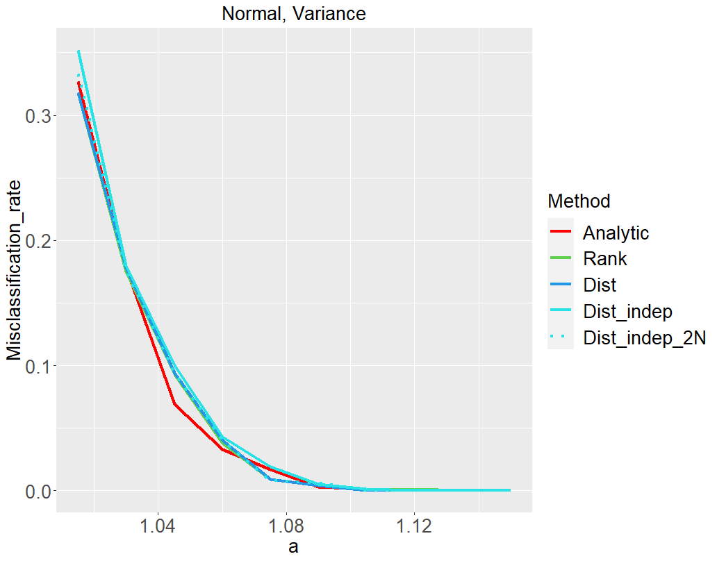
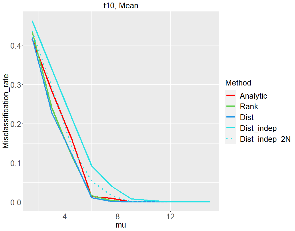
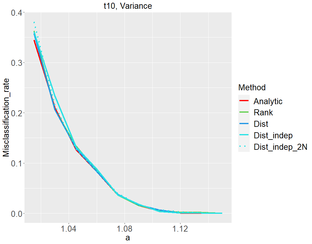
Figure 7: Analytic and simulated misclassification rates in scenario 10 (upper-left panel), scenario 11 (upper-right panel), scenario 12 (bottom-left panel), scenario 13 (bottom-right panel).

The authors were supported in part by the NSF and DMS-1848579.

References

- Ayyad, Saleh and Labib (2019) {barticle}[author] \bauthor\bsnmAyyad, \bfnmSarah M\binitsS. M., \bauthor\bsnmSaleh, \bfnmAhmed I\binitsA. I. and \bauthor\bsnmLabib, \bfnmLabib M\binitsL. M. (\byear2019). \btitleGene expression cancer classification using modified K-Nearest Neighbors technique. \bjournalBiosystems \bvolume176 \bpages41–51. \endbibitem
- Bansal and Srivastava (2018) {barticle}[author] \bauthor\bsnmBansal, \bfnmBarkha\binitsB. and \bauthor\bsnmSrivastava, \bfnmSangeet\binitsS. (\byear2018). \btitleSentiment classification of online consumer reviews using word vector representations. \bjournalProcedia computer science \bvolume132 \bpages1147–1153. \endbibitem
- Boser, Guyon and Vapnik (1992) {binproceedings}[author] \bauthor\bsnmBoser, \bfnmBernhard E\binitsB. E., \bauthor\bsnmGuyon, \bfnmIsabelle M\binitsI. M. and \bauthor\bsnmVapnik, \bfnmVladimir N\binitsV. N. (\byear1992). \btitleA training algorithm for optimal margin classifiers. In \bbooktitleProceedings of the fifth annual workshop on Computational learning theory \bpages144–152. \endbibitem
- Breiman (2001) {barticle}[author] \bauthor\bsnmBreiman, \bfnmLeo\binitsL. (\byear2001). \btitleRandom forests. \bjournalMachine learning \bvolume45 \bpages5–32. \endbibitem
- Brown et al. (1999) {barticle}[author] \bauthor\bsnmBrown, \bfnmM\binitsM., \bauthor\bsnmGrundy, \bfnmWilliam Noble\binitsW. N., \bauthor\bsnmLin, \bfnmDavid\binitsD., \bauthor\bsnmCristianini, \bfnmNello\binitsN., \bauthor\bsnmSugnet, \bfnmCharles\binitsC., \bauthor\bsnmAres, \bfnmManuel\binitsM. and \bauthor\bsnmHaussler, \bfnmDavid\binitsD. (\byear1999). \btitleSupport vector machine classification of microarray gene expression data. \bjournalUniversity of California, Santa Cruz, Technical Report UCSC-CRL-99-09. \endbibitem
- Buehlmann (2006) {barticle}[author] \bauthor\bsnmBuehlmann, \bfnmPeter\binitsP. (\byear2006). \btitleBoosting for high-dimensional linear models. \bjournalThe Annals of Statistics \bvolume34 \bpages559–583. \endbibitem
- Burkhardt et al. (2010) {binproceedings}[author] \bauthor\bsnmBurkhardt, \bfnmFelix\binitsF., \bauthor\bsnmEckert, \bfnmMartin\binitsM., \bauthor\bsnmJohannsen, \bfnmWiebke\binitsW. and \bauthor\bsnmStegmann, \bfnmJoachim\binitsJ. (\byear2010). \btitleA Database of Age and Gender Annotated Telephone Speech. In \bbooktitleLREC. \bpublisherMalta. \endbibitem
- Chen, Chen and Deng (2019) {barticle}[author] \bauthor\bsnmChen, \bfnmHao\binitsH., \bauthor\bsnmChen, \bfnmShizhe\binitsS. and \bauthor\bsnmDeng, \bfnmXinyi\binitsX. (\byear2019). \btitleA universal nonparametric event detection framework for neuropixels data. \bjournalbioRxiv \bpages650671. \endbibitem
- Chen and Friedman (2017) {barticle}[author] \bauthor\bsnmChen, \bfnmHao\binitsH. and \bauthor\bsnmFriedman, \bfnmJerome H\binitsJ. H. (\byear2017). \btitleA new graph-based two-sample test for multivariate and object data. \bjournalJournal of the American statistical association \bvolume112 \bpages397–409. \endbibitem
- Cover and Hart (1967) {barticle}[author] \bauthor\bsnmCover, \bfnmThomas\binitsT. and \bauthor\bsnmHart, \bfnmPeter\binitsP. (\byear1967). \btitleNearest neighbor pattern classification. \bjournalIEEE transactions on information theory \bvolume13 \bpages21–27. \endbibitem
- Fan and Fan (2008) {barticle}[author] \bauthor\bsnmFan, \bfnmJianqing\binitsJ. and \bauthor\bsnmFan, \bfnmYingying\binitsY. (\byear2008). \btitleHigh dimensional classification using features annealed independence rules. \bjournalAnnals of statistics \bvolume36 \bpages2605. \endbibitem
- Fernández-Delgado et al. (2014) {barticle}[author] \bauthor\bsnmFernández-Delgado, \bfnmManuel\binitsM., \bauthor\bsnmCernadas, \bfnmEva\binitsE., \bauthor\bsnmBarro, \bfnmSenén\binitsS. and \bauthor\bsnmAmorim, \bfnmDinani\binitsD. (\byear2014). \btitleDo we need hundreds of classifiers to solve real world classification problems? \bjournalThe journal of machine learning research \bvolume15 \bpages3133–3181. \endbibitem
- Fisher (1936) {barticle}[author] \bauthor\bsnmFisher, \bfnmRonald A\binitsR. A. (\byear1936). \btitleThe use of multiple measurements in taxonomic problems. \bjournalAnnals of eugenics \bvolume7 \bpages179–188. \endbibitem
- Freund et al. (1996) {binproceedings}[author] \bauthor\bsnmFreund, \bfnmYoav\binitsY., \bauthor\bsnmSchapire, \bfnmRobert E\binitsR. E. \betalet al. (\byear1996). \btitleExperiments with a new boosting algorithm. In \bbooktitleicml \bvolume96 \bpages148–156. \bpublisherCiteseer. \endbibitem
- Furey et al. (2000) {barticle}[author] \bauthor\bsnmFurey, \bfnmTerrence S\binitsT. S., \bauthor\bsnmCristianini, \bfnmNello\binitsN., \bauthor\bsnmDuffy, \bfnmNigel\binitsN., \bauthor\bsnmBednarski, \bfnmDavid W\binitsD. W., \bauthor\bsnmSchummer, \bfnmMichel\binitsM. and \bauthor\bsnmHaussler, \bfnmDavid\binitsD. (\byear2000). \btitleSupport vector machine classification and validation of cancer tissue samples using microarray expression data. \bjournalBioinformatics \bvolume16 \bpages906–914. \endbibitem
- Ghaddar and Naoum-Sawaya (2018) {barticle}[author] \bauthor\bsnmGhaddar, \bfnmBissan\binitsB. and \bauthor\bsnmNaoum-Sawaya, \bfnmJoe\binitsJ. (\byear2018). \btitleHigh dimensional data classification and feature selection using support vector machines. \bjournalEuropean Journal of Operational Research \bvolume265 \bpages993–1004. \endbibitem
- Golub et al. (1999) {barticle}[author] \bauthor\bsnmGolub, \bfnmTodd R\binitsT. R., \bauthor\bsnmSlonim, \bfnmDonna K\binitsD. K., \bauthor\bsnmTamayo, \bfnmPablo\binitsP., \bauthor\bsnmHuard, \bfnmChristine\binitsC., \bauthor\bsnmGaasenbeek, \bfnmMichelle\binitsM., \bauthor\bsnmMesirov, \bfnmJill P\binitsJ. P., \bauthor\bsnmColler, \bfnmHilary\binitsH., \bauthor\bsnmLoh, \bfnmMignon L\binitsM. L., \bauthor\bsnmDowning, \bfnmJames R\binitsJ. R., \bauthor\bsnmCaligiuri, \bfnmMark A\binitsM. A. \betalet al. (\byear1999). \btitleMolecular classification of cancer: class discovery and class prediction by gene expression monitoring. \bjournalscience \bvolume286 \bpages531–537. \endbibitem
- Hussain (2019) {barticle}[author] \bauthor\bsnmHussain, \bfnmSyed Fawad\binitsS. F. (\byear2019). \btitleA novel robust kernel for classifying high-dimensional data using Support Vector Machines. \bjournalExpert Systems with Applications \bvolume131 \bpages116–131. \endbibitem
- Leathwick et al. (2005) {barticle}[author] \bauthor\bsnmLeathwick, \bfnmJR\binitsJ., \bauthor\bsnmRowe, \bfnmD\binitsD., \bauthor\bsnmRichardson, \bfnmJ\binitsJ., \bauthor\bsnmElith, \bfnmJane\binitsJ. and \bauthor\bsnmHastie, \bfnmT\binitsT. (\byear2005). \btitleUsing multivariate adaptive regression splines to predict the distributions of New Zealand’s freshwater diadromous fish. \bjournalFreshwater Biology \bvolume50 \bpages2034–2052. \endbibitem
- LeCun et al. (1989) {barticle}[author] \bauthor\bsnmLeCun, \bfnmYann\binitsY., \bauthor\bsnmBoser, \bfnmBernhard\binitsB., \bauthor\bsnmDenker, \bfnmJohn S\binitsJ. S., \bauthor\bsnmHenderson, \bfnmDonnie\binitsD., \bauthor\bsnmHoward, \bfnmRichard E\binitsR. E., \bauthor\bsnmHubbard, \bfnmWayne\binitsW. and \bauthor\bsnmJackel, \bfnmLawrence D\binitsL. D. (\byear1989). \btitleBackpropagation applied to handwritten zip code recognition. \bjournalNeural computation \bvolume1 \bpages541–551. \endbibitem
- Li, Zhang and Jiang (2005) {binproceedings}[author] \bauthor\bsnmLi, \bfnmHaifeng\binitsH., \bauthor\bsnmZhang, \bfnmKeshu\binitsK. and \bauthor\bsnmJiang, \bfnmTao\binitsT. (\byear2005). \btitleRobust and accurate cancer classification with gene expression profiling. In \bbooktitle2005 IEEE Computational Systems Bioinformatics Conference (CSB’05) \bpages310–321. \bpublisherIEEE. \endbibitem
- Liu et al. (2006) {barticle}[author] \bauthor\bsnmLiu, \bfnmTing\binitsT., \bauthor\bsnmMoore, \bfnmAndrew W\binitsA. W., \bauthor\bsnmGray, \bfnmAlexander\binitsA. and \bauthor\bsnmCardie, \bfnmClaire\binitsC. (\byear2006). \btitleNew algorithms for efficient high-dimensional nonparametric classification. \bjournalJournal of Machine Learning Research \bvolume7. \endbibitem
- Maa, Pearl and Bartoszyński (1996) {barticle}[author] \bauthor\bsnmMaa, \bfnmJen-Fue\binitsJ.-F., \bauthor\bsnmPearl, \bfnmDennis K\binitsD. K. and \bauthor\bsnmBartoszyński, \bfnmRobert\binitsR. (\byear1996). \btitleReducing multidimensional two-sample data to one-dimensional interpoint comparisons. \bjournalThe annals of statistics \bvolume24 \bpages1069–1074. \endbibitem
- Martens and Naes (1992) {bbook}[author] \bauthor\bsnmMartens, \bfnmHarald\binitsH. and \bauthor\bsnmNaes, \bfnmTormod\binitsT. (\byear1992). \btitleMultivariate calibration. \bpublisherJohn Wiley & Sons. \endbibitem
- Mayr et al. (2012) {barticle}[author] \bauthor\bsnmMayr, \bfnmAndreas\binitsA., \bauthor\bsnmFenske, \bfnmNora\binitsN., \bauthor\bsnmHofner, \bfnmBenjamin\binitsB., \bauthor\bsnmKneib, \bfnmThomas\binitsT. and \bauthor\bsnmSchmid, \bfnmMatthias\binitsM. (\byear2012). \btitleGeneralized additive models for location, scale and shape for high dimensional data—a flexible approach based on boosting. \bjournalJournal of the Royal Statistical Society: Series C (Applied Statistics) \bvolume61 \bpages403–427. \endbibitem
- Pal, Mondal and Ghosh (2016) {barticle}[author] \bauthor\bsnmPal, \bfnmArnab K\binitsA. K., \bauthor\bsnmMondal, \bfnmPronoy K\binitsP. K. and \bauthor\bsnmGhosh, \bfnmAnil K\binitsA. K. (\byear2016). \btitleHigh dimensional nearest neighbor classification based on mean absolute differences of inter-point distances. \bjournalPattern Recognition Letters \bvolume74 \bpages1–8. \endbibitem
- Paliwal and Sharma (2012) {barticle}[author] \bauthor\bsnmPaliwal, \bfnmKuldip K\binitsK. K. and \bauthor\bsnmSharma, \bfnmAlok\binitsA. (\byear2012). \btitleImproved pseudoinverse linear discriminant analysis method for dimensionality reduction. \bjournalInternational Journal of Pattern Recognition and Artificial Intelligence \bvolume26 \bpages1250002. \endbibitem
- Raič (2019) {barticle}[author] \bauthor\bsnmRaič, \bfnmMartin\binitsM. (\byear2019). \btitleA multivariate Berry–Esseen theorem with explicit constants. \endbibitem
- Ranzato et al. (2006) {barticle}[author] \bauthor\bsnmRanzato, \bfnmMarc’Aurelio\binitsM., \bauthor\bsnmPoultney, \bfnmChristopher\binitsC., \bauthor\bsnmChopra, \bfnmSumit\binitsS. and \bauthor\bsnmCun, \bfnmYann\binitsY. (\byear2006). \btitleEfficient learning of sparse representations with an energy-based model. \bjournalAdvances in neural information processing systems \bvolume19. \endbibitem
- Rao (1948) {barticle}[author] \bauthor\bsnmRao, \bfnmC Radhakrishna\binitsC. R. (\byear1948). \btitleThe utilization of multiple measurements in problems of biological classification. \bjournalJournal of the Royal Statistical Society. Series B (Methodological) \bvolume10 \bpages159–203. \endbibitem
- Salzberg (1994) {bmisc}[author] \bauthor\bsnmSalzberg, \bfnmSteven L\binitsS. L. (\byear1994). \btitleC4. 5: Programs for machine learning by j. ross quinlan. morgan kaufmann publishers, inc., 1993. \endbibitem
- Schölkopf et al. (2001) {barticle}[author] \bauthor\bsnmSchölkopf, \bfnmBernhard\binitsB., \bauthor\bsnmPlatt, \bfnmJohn C\binitsJ. C., \bauthor\bsnmShawe-Taylor, \bfnmJohn\binitsJ., \bauthor\bsnmSmola, \bfnmAlex J\binitsA. J. and \bauthor\bsnmWilliamson, \bfnmRobert C\binitsR. C. (\byear2001). \btitleEstimating the support of a high-dimensional distribution. \bjournalNeural computation \bvolume13 \bpages1443–1471. \endbibitem
- Shi et al. (2015) {barticle}[author] \bauthor\bsnmShi, \bfnmXingjian\binitsX., \bauthor\bsnmChen, \bfnmZhourong\binitsZ., \bauthor\bsnmWang, \bfnmHao\binitsH., \bauthor\bsnmYeung, \bfnmDit-Yan\binitsD.-Y., \bauthor\bsnmWong, \bfnmWai-Kin\binitsW.-K. and \bauthor\bsnmWoo, \bfnmWang-chun\binitsW.-c. (\byear2015). \btitleConvolutional LSTM network: A machine learning approach for precipitation nowcasting. \bjournalAdvances in neural information processing systems \bvolume28. \endbibitem
- Stringer et al. (2019) {barticle}[author] \bauthor\bsnmStringer, \bfnmCarsen\binitsC., \bauthor\bsnmPachitariu, \bfnmMarius\binitsM., \bauthor\bsnmSteinmetz, \bfnmNicholas\binitsN., \bauthor\bsnmReddy, \bfnmCharu Bai\binitsC. B., \bauthor\bsnmCarandini, \bfnmMatteo\binitsM. and \bauthor\bsnmHarris, \bfnmKenneth D\binitsK. D. (\byear2019). \btitleSpontaneous behaviors drive multidimensional, brainwide activity. \bjournalScience \bvolume364. \endbibitem
- Tang et al. (2011) {binproceedings}[author] \bauthor\bsnmTang, \bfnmLu-An\binitsL.-A., \bauthor\bsnmZheng, \bfnmYu\binitsY., \bauthor\bsnmXie, \bfnmXing\binitsX., \bauthor\bsnmYuan, \bfnmJing\binitsJ., \bauthor\bsnmYu, \bfnmXiao\binitsX. and \bauthor\bsnmHan, \bfnmJiawei\binitsJ. (\byear2011). \btitleRetrieving k-nearest neighboring trajectories by a set of point locations. In \bbooktitleInternational Symposium on Spatial and Temporal Databases \bpages223–241. \bpublisherSpringer. \endbibitem
- Yang and Wu (2014) {barticle}[author] \bauthor\bsnmYang, \bfnmWuyi\binitsW. and \bauthor\bsnmWu, \bfnmHouyuan\binitsH. (\byear2014). \btitleRegularized complete linear discriminant analysis. \bjournalNeurocomputing \bvolume137 \bpages185–191. \endbibitem
- Ye, Zhang and Law (2009) {barticle}[author] \bauthor\bsnmYe, \bfnmQiang\binitsQ., \bauthor\bsnmZhang, \bfnmZiqiong\binitsZ. and \bauthor\bsnmLaw, \bfnmRob\binitsR. (\byear2009). \btitleSentiment classification of online reviews to travel destinations by supervised machine learning approaches. \bjournalExpert systems with applications \bvolume36 \bpages6527–6535. \endbibitem
- Ye et al. (2013) {barticle}[author] \bauthor\bsnmYe, \bfnmYunming\binitsY., \bauthor\bsnmWu, \bfnmQingyao\binitsQ., \bauthor\bsnmHuang, \bfnmJoshua Zhexue\binitsJ. Z., \bauthor\bsnmNg, \bfnmMichael K\binitsM. K. and \bauthor\bsnmLi, \bfnmXutao\binitsX. (\byear2013). \btitleStratified sampling for feature subspace selection in random forests for high dimensional data. \bjournalPattern Recognition \bvolume46 \bpages769–787. \endbibitem