One-class systems seamlessly fit in the forward-forward algorithm

Abstract

The forward-forward algorithm [Hinton, 2022] presents a new method of training neural networks by updating weights during an inference, performing parameter updates for each layer individually. This immediately reduces memory requirements during training and may lead to many more benefits, like seamless online training. This method relies on a loss ("goodness") function that can be evaluated on the activations of each layer, of which can have a varied parameter size, depending on the hyperparamaterization of the network. In the seminal paper, a goodness function was proposed to fill this need; however, if placed in a one-class problem context, one need not pioneer a new loss because these functions can innately handle dynamic network sizes. In this paper, we investigate the performance of deep one-class objective functions when trained in a forward-forward fashion. The code is available at https://github.com/MichaelHopwood/ForwardForwardOneclass.

1 Introduction

The Forward-Forward algorithm [Hinton, 2022] is a new learning procedure for neural networks that updates network parameters immediately after the forward pass of a layer. An objective (aka, "goodness") function is evaluated on the layer’s latent output representations $G(h^{[l]}|\mathcal{I})$ conditioned upon some data integrity $\mathcal{I}$. Integrity is broken down into positive and negative data; positive data is often thought of as correct data while negative data is incorrect data. When positive data is passed into the model, weights that support the data (aka, neurons that fire with large weights) are awarded. The assignment of these positive and negative data is subject to creativity with one of the most common practices being placing incorrect class assignments in the negative data.

In a one-class problem context, it is assumed that the majority of the training dataset consists of “normal” data, and the model is assigned with determining the normality of the input data. Therefore, negative data is not required, and the objective function can be simplified to $G(h^{[l]})$. Many deep learning methods answer this anomaly detection problem via inspirations from support vector machines [Cortes and Vapnik, 1995] like Deep SVDD [Ruff et al., 2018] or Deep OC-SVM [Sohn et al., 2020].

2 Methodology

For a layer $l$ we compute a forward pass

$$h^{[l]}=\hbox{ReLU}\left(xW^{[l]}+b^{[l]}\right)$$

where $x\in\mathbb{R}^{n,p}$ is the data from the previous layer, $h\in\mathbb{R}^{n,q}$ is the transformed data, and $W^{[l]}\in\mathbb{R}^{p,q}$ and $b^{[l]}\in\mathbb{R}^{q}$ are the trained weights and biases. A forward pass of normal class data can be used to calculate the loss function at layer $l$ following some $G(h^{[l]})$. These $G(h^{[l]})$ can be any convex function; in the following table, we produce some candidate goodness functions.

Method	Derivation
Goodness	$\begin{aligned} \mathcal{L}(h^{[l]};\mathcal{W})=\sum_{i=1}^{N}\sigma(||h^{[l]}||^{2}-C)\end{aligned}$
GoodnessAdjusted	$\begin{aligned} \mathcal{L}(h^{[l]};\mathcal{W})=\sum_{i=1}^{N}\log(1+\exp(||h||^{2}-C))\end{aligned}$
HB-SVDD	$\begin{aligned} \mathcal{L}(h^{[l]};\mathcal{W})=\sum_{i=1}^{N}||h^{[l]}-\mathbf{a}||^{2}\end{aligned}$
SVDD [Ruff et al., 2018]	$\begin{aligned} &\underset{\mathbf{a},R,\xi_{i}}{\text{minimize}}\hskip 11.38092ptR^{2}+C\sum_{i=1}^{N}\xi_{i}\\ &\text{subject to}\hskip 8.5359pt||h^{[l]}-\mathbf{a}||^{2}\leq R^{2}+\xi_{i},\hskip 14.22636pti=1,2,...,N\\ &\text{and}\hskip 36.98866pt\xi_{i}\geq 0,\hskip 62.59596pti=1,2,...,N\\ \cline{1-2}\cr&\mathcal{L}(h^{[l]};R,\mathcal{W})=R^{2}+C\sum_{i=1}^{N}\max\bigl{(}0,||h^{[l]}-\mathbf{a}||^{2}-R^{2}\bigr{)}\end{aligned}$
LS-SVDD	$\begin{aligned} &\underset{R,\mathbf{a},\xi_{i}}{\text{minimize}}\hskip 11.38092ptR^{2}+\frac{C}{2}\sum_{i=1}^{N}\xi_{i}^{2}\\ &\text{subject to}\hskip 8.5359pt||h^{[l]}-\mathbf{a}||=R^{2}+\xi_{i},\hskip 14.22636pti=1,2,...,N\\ \cline{1-2}\cr&\mathcal{L}(h^{[l]};R,\mathcal{W})=R^{2}+\frac{C}{2}\sum_{i=1}^{N}\Bigl{(}||h^{[l]}-\mathbf{a}||^{2}-R^{2}\Bigr{)}^{2}\end{aligned}$

Table 1: Derivations of deep learning one-class "goodness" functions. Note that $\mathbf{a}=\frac{1}{N}\sum_{i=1}^{N}h^{[l]}_{i,j}$.

The network’s weights are updated sequentially, where inputs $h^{[l-1]}$ are passed through the layer to compute $h^{[l]}$, the loss $\mathcal{L}(h^{[l]})$ is calculated, and used to backpropagate using gradient descent

$$W^{[l]} =W^{[l]}+\frac{\lambda}{n}\frac{\partial G}{\partial W^{[l]}}$$

$$b^{[l]} =b^{[l]}+\frac{\lambda}{n}\frac{\partial G}{\partial b^{[l]}}$$

To convert the final embeddings $h^{[L]}\in\mathbb{R}^{n\times q}$ into an outlier probability, we pass them into the loss function to ascertain a distance value $D=\mathcal{L}(h^{[L]})\in\mathbb{R}^{n}$ for each sample and then convert these distances to probabilities by normalizing by the maximum value, so $P=\frac{D}{\max(D)}\in\mathbb{R}^{n}$. In order to deem the sample an outlier, a threshold is deduced during training by evaluating $t=P_{(1-\nu)th\%}$. Therefore, an outlier is flagged via $I_{P>t}$. We utilize a $\nu=0.05$ for all settings. This method of ascertaining a threshold naturally reduces our chances of achieving 100% accuracy, but it also reduces the chances of a type 2 error, which is important for outlier detection problems.

The code is written in PyTorch to leverage its built-in autodifferentiation tool. For the Forward-Forward implementation, gradients are computed at the end of each layer and the weights are updated according to the calculated autodifferentiated gradients and the optimizer. The normal backpropagation implmenetation conducts the weight update process for the weights in all layers after completing the forward pass on the last layer. So, while the forward-forward implementation has $L$ instantiated optimizers, the normal backpropagation method has 1 instantiated optimizer. For both cases, a stochastic gradient descent optimizer was used with no momentum and weight decay (see equations above). Early stopping is implemented by checking whether the backpropagation

In order to make the experiments reproducible, random seeds were implemented. Across the 50 independent trials which were run for each parameter setting, a seed was $s=1...50$ was used when initializing the model parameters (e.g. weights and biases). For all independent trials, the same data split (e.g. train, valid, test) was used. This step is imperative, especially given the importance of the weight initialization for oneclass problem settings.

2.1 Data

The banknote authentication dataset [Dua and Graff, 2017] was used for evaluating the different methods. This data comprises images of both authentic and counterfeit banknotes captured using an industrial camera typically utilized for print inspection. The resulting images had a resolution of 400 x 400 pixels, and due to the object lens and distance to the subject, grayscale images with a resolution of approximately 660 dpi were obtained. The Wavelet Transform tool was employed to extract features from the images, resulting in 4 continuous features total, 3 features containing statistics of the Wavelet Transformed image (variance, skewness, kurtosis), and also the entropy of the image. The response variable is a binary value; 610 of the 1372 samples were deemed fake.

2.2 Evaluation

This data was split into train, validation, and test splits. The training data trained the network weights. The validation data was used to decide early stopping. The test data was used to evaluate the model using accuracy, F1, and AUC. A grid search was conducted across the 5 loss functions (Table 1), across 4 neural network architectures. Each setting was evaluated using 50 independent tests across different seeds, which impacted the network random initializations.

3 Results

3.1 Forward Forward (FF) v. Normal Backpropagation (BP)

The tabulated results are provided in Tables 2 & 3. The average accuracy for all experiments using BP was 57.6047%; the FF experiments had an average value of 56.6287%. Therefore, on average, BP experiments were 1% more accurate. Similarly, BP was around 0.01 (i.e. 1%) better in AUC with average BP and FF values of 0.549 and 0.538, Additionally, BP was around 0.025 (i.e. 2.5%) better in the F1 score with average BP and FF values of 0.299 and 0.276. respectively. However, given the volatility of training deep oneclass models, it is worthwhile to compare the performance of the best models as opposed to the average model performance. Looking at all metrics, the best models achieve higher performance when trained using a FF pipeline; accuracy improves from 93.45% to 94.18%, F1 score improves from 0.9274 to 0.9375, and AUC improves from 0.9354 to 0.9461.

3.2 Loss function evaluation

In the forward forward evaluations, all of the best models used the goodness functions. They also perform well on average, with two of the three metrics having the highest average model performance when using them. Interestingly, the backpropagation evaluations all perform the best when using an LS-SVDD loss.

4 Conclusion

In summary, the following conclusions were made:

1. For one-class problems, forward-forward training shows comparable results to normal backpropagation in this case study (Table 2 and Table 3)

2. The goodness function is a viable loss candidate for one-class models (Table 2 and Table 3)

3. Forward-forward seemlessly enables the visualization of loss landscapes within the network, which can help gain insights into the learning process (Figure 1)

Future work should be conducted to expand this study to deeper models and more benchmark data. Additionally, when training one-class problems using neural networks, many implementations find that pretraining the network weights using autoencoders are helpful, and sometimes, essential. Lastly, further work can introduce autoencoders into the training pipeline to regulate the model results across different random seeds.

Appendix A Appendix

	Accuracy (%)		F1		AUC
Method	$\mu(\pm\sigma)$	$\max$	$\mu(\pm\sigma)$	$\max$	$\mu(\pm\sigma)$	$\max$
Goodness (4,10,10)	60.04 ($\pm$ 10.15 )	89.82	0.2568 ($\pm$ 0.2681)	0.8923	0.5598 ($\pm$ 0.115)	0.9035
Goodness (4,25,25)	59.49 ($\pm$ 10.14 )	93.82	0.2319 ($\pm$ 0.2686)	0.9333	0.5529 ($\pm$ 0.1153)	0.942
Goodness (4,50,50)	63.23 ($\pm$ 12.41 )	92.73	0.3273 ($\pm$ 0.3099)	0.916	0.5949 ($\pm$ 0.1392)	0.9238
Goodness (4,100,100)	65.21 ($\pm$ 13.95 )	88.0	0.3704 ($\pm$ 0.3367)	0.8629	0.6177 ($\pm$ 0.1567)	0.8764
GoodnessAdjusted (4,10,10)	59.81 ($\pm$ 10.04 )	89.82	0.2491 ($\pm$ 0.2639)	0.8923	0.557 ($\pm$ 0.1136)	0.9035
GoodnessAdjusted (4,25,25)	59.56 ($\pm$ 9.98 )	94.18	0.2384 ($\pm$ 0.2667)	0.9375	0.5541 ($\pm$ 0.1133)	0.9461
GoodnessAdjusted (4,50,50)	62.16 ($\pm$ 12.37 )	90.55	0.3082 ($\pm$ 0.3035)	0.8879	0.5836 ($\pm$ 0.1384)	0.8993
GoodnessAdjusted (4,100,100)	63.69 ($\pm$ 13.92 )	91.64	0.3372 ($\pm$ 0.3289)	0.9046	0.601 ($\pm$ 0.1554)	0.914
HB-SVDD (4,10,10)	57.14 ($\pm$ 5.89 )	76.36	0.1853 ($\pm$ 0.1757)	0.6829	0.5261 ($\pm$ 0.0659)	0.7444
HB-SVDD (4,25,25)	57.99 ($\pm$ 7.5 )	80.36	0.2107 ($\pm$ 0.2154)	0.7523	0.5363 ($\pm$ 0.0844)	0.7903
HB-SVDD (4,50,50)	60.6 ($\pm$ 9.05 )	86.18	0.298 ($\pm$ 0.2322)	0.8376	0.5669 ($\pm$ 0.101)	0.8559
HB-SVDD (4,100,100)	58.29 ($\pm$ 8.27 )	80.73	0.2322 ($\pm$ 0.227)	0.7558	0.541 ($\pm$ 0.0919)	0.7936
SVDD (4,10,10)	48.2 ($\pm$ 5.4 )	61.09	0.4169 ($\pm$ 0.2699)	0.6146	0.4993 ($\pm$ 0.0167)	0.5615
SVDD (4,25,25)	47.64 ($\pm$ 5.45 )	61.45	0.4539 ($\pm$ 0.2527)	0.6146	0.5004 ($\pm$ 0.0208)	0.5656
SVDD (4,50,50)	46.21 ($\pm$ 4.47 )	60.0	0.5328 ($\pm$ 0.1922)	0.6146	0.5013 ($\pm$ 0.0139)	0.5509
SVDD (4,100,100)	47.6 ($\pm$ 6.13 )	62.91	0.5011 ($\pm$ 0.2094)	0.6146	0.5067 ($\pm$ 0.0234)	0.582
LS-SVDD (4,10,10)	54.97 ($\pm$ 5.15 )	71.64	0.138 ($\pm$ 0.1439)	0.6174	0.5032 ($\pm$ 0.0559)	0.6853
LS-SVDD (4,25,25)	53.94 ($\pm$ 3.72 )	69.45	0.1074 ($\pm$ 0.1137)	0.5484	0.4917 ($\pm$ 0.0399)	0.6665
LS-SVDD (4,50,50)	53.24 ($\pm$ 2.66 )	57.09	0.0691 ($\pm$ 0.0692)	0.2561	0.4828 ($\pm$ 0.024)	0.5206
LS-SVDD (4,100,100)	53.56 ($\pm$ 2.13 )	57.45	0.0537 ($\pm$ 0.0569)	0.183	0.4845 ($\pm$ 0.0202)	0.523

Table 2: Results across 50 independent trials. Forward forward. Seed controlled.

	Accuracy (%)		F1		AUC
Method	$\mu(\pm\sigma)$	$\max$	$\mu(\pm\sigma)$	$\max$	$\mu(\pm\sigma)$	$\max$
Goodness (4,10,10)	60.92 ($\pm$ 11.44 )	90.18	0.2705 ($\pm$ 0.2917)	0.8898	0.5695 ($\pm$ 0.1295)	0.901
Goodness (4,25,25)	59.82 ($\pm$ 10.37 )	91.27	0.2341 ($\pm$ 0.2771)	0.9062	0.5564 ($\pm$ 0.1185)	0.9166
Goodness (4,50,50)	62.97 ($\pm$ 12.2 )	91.27	0.3219 ($\pm$ 0.3061)	0.8966	0.5919 ($\pm$ 0.1367)	0.9066
Goodness (4,100,100)	65.22 ($\pm$ 13.97 )	88.0	0.3703 ($\pm$ 0.3371)	0.8629	0.6178 ($\pm$ 0.157)	0.8764
GoodnessAdjusted (4,10,10)	61.08 ($\pm$ 11.53 )	90.18	0.2742 ($\pm$ 0.2922)	0.8898	0.5713 ($\pm$ 0.1305)	0.901
GoodnessAdjusted (4,25,25)	59.87 ($\pm$ 10.17 )	90.91	0.237 ($\pm$ 0.2737)	0.902	0.5569 ($\pm$ 0.1162)	0.9125
GoodnessAdjusted (4,50,50)	62.88 ($\pm$ 12.16 )	90.91	0.3203 ($\pm$ 0.3048)	0.8918	0.5909 ($\pm$ 0.1363)	0.9025
GoodnessAdjusted (4,100,100)	66.23 ($\pm$ 14.11 )	90.91	0.3951 ($\pm$ 0.3409)	0.898	0.6292 ($\pm$ 0.1586)	0.9083
HB-SVDD (4,10,10)	57.43 ($\pm$ 5.89 )	78.18	0.1987 ($\pm$ 0.1705)	0.717	0.5295 ($\pm$ 0.0654)	0.7657
HB-SVDD (4,25,25)	58.71 ($\pm$ 7.99 )	79.27	0.236 ($\pm$ 0.2227)	0.6984	0.5449 ($\pm$ 0.0894)	0.7672
HB-SVDD (4,50,50)	61.35 ($\pm$ 9.85 )	86.55	0.3238 ($\pm$ 0.2446)	0.8412	0.5762 ($\pm$ 0.1096)	0.8592
HB-SVDD (4,100,100)	59.06 ($\pm$ 8.66 )	80.36	0.2546 ($\pm$ 0.2337)	0.7453	0.5497 ($\pm$ 0.0961)	0.7878
SVDD (4,10,10)	47.43 ($\pm$ 5.01 )	60.73	0.4472 ($\pm$ 0.2612)	0.6146	0.4981 ($\pm$ 0.0173)	0.5574
SVDD (4,25,25)	48.22 ($\pm$ 6.02 )	61.82	0.4514 ($\pm$ 0.2462)	0.6146	0.5041 ($\pm$ 0.0219)	0.5697
SVDD (4,50,50)	46.74 ($\pm$ 5.01 )	60.0	0.5128 ($\pm$ 0.2091)	0.6146	0.5023 ($\pm$ 0.0155)	0.5542
SVDD (4,100,100)	48.49 ($\pm$ 6.68 )	63.27	0.4737 ($\pm$ 0.2233)	0.6146	0.5092 ($\pm$ 0.0252)	0.5861
LS-SVDD (4,10,10)	57.48 ($\pm$ 7.25 )	77.45	0.2126 ($\pm$ 0.2127)	0.7438	0.5327 ($\pm$ 0.0818)	0.7708
LS-SVDD (4,25,25)	57.77 ($\pm$ 7.51 )	93.45	0.2064 ($\pm$ 0.1991)	0.9274	0.5338 ($\pm$ 0.0842)	0.9354
LS-SVDD (4,50,50)	56.11 ($\pm$ 6.1 )	84.36	0.1418 ($\pm$ 0.1737)	0.8201	0.514 ($\pm$ 0.0689)	0.8395
LS-SVDD (4,100,100)	54.33 ($\pm$ 4.15 )	72.0	0.115 ($\pm$ 0.1118)	0.5838	0.4955 ($\pm$ 0.0434)	0.6919

Table 3: Results across 50 independent trials. Backpropagation. Seed controlled.

a)

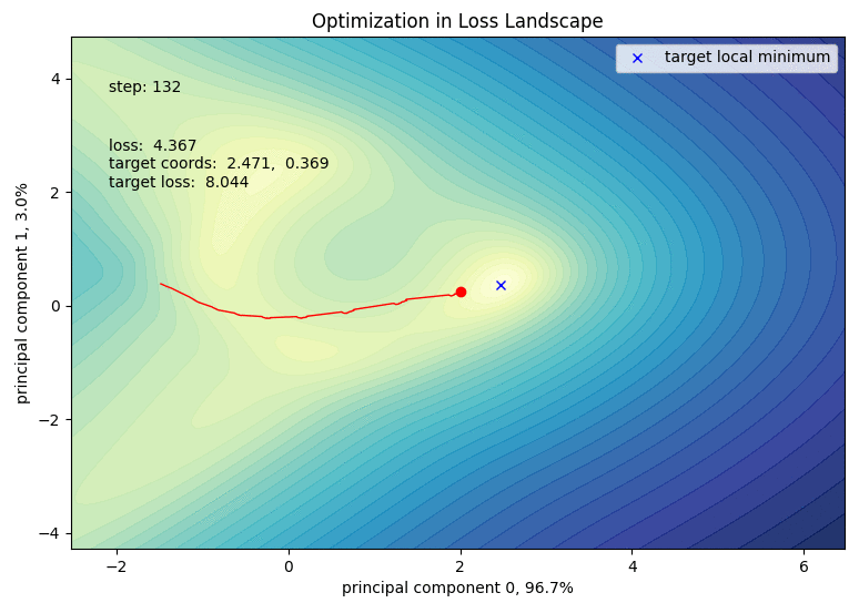
b)

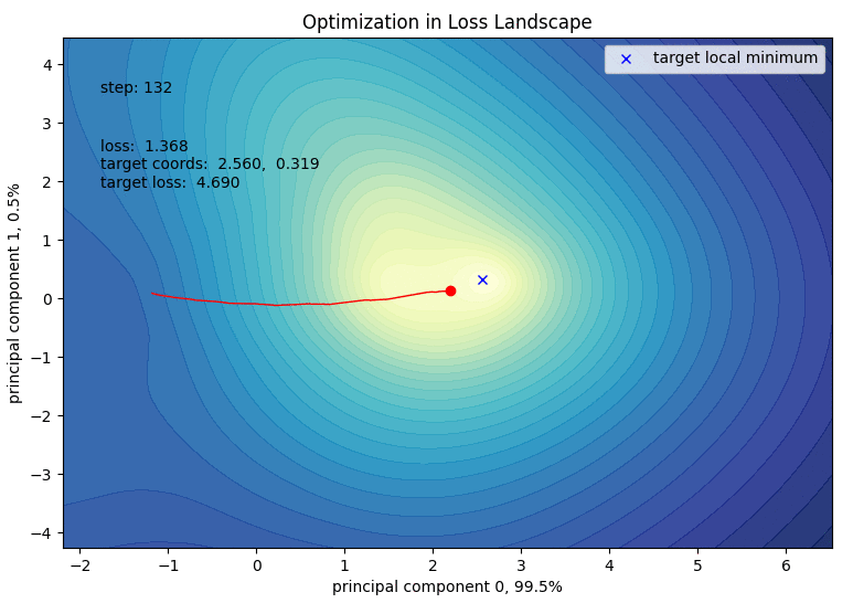
Figure 1: Loss landscapes for the neural network’s a) first layer, and b) second layer when trained via forward-forward with a LS-SVDD loss.

References

- [Cortes and Vapnik, 1995] Cortes, C. and Vapnik, V. (1995). Support-vector networks. Machine learning, 20:273–297.
- [Dua and Graff, 2017] Dua, D. and Graff, C. (2017). UCI machine learning repository.
- [Hinton, 2022] Hinton, G. (2022). The forward-forward algorithm: Some preliminary investigations. arXiv preprint arXiv:2212.13345.
- [Ruff et al., 2018] Ruff, L., Vandermeulen, R., Goernitz, N., Deecke, L., Siddiqui, S. A., Binder, A., Müller, E., and Kloft, M. (2018). Deep one-class classification. In International conference on machine learning, pages 4393–4402. PMLR.
- [Sohn et al., 2020] Sohn, K., Li, C.-L., Yoon, J., Jin, M., and Pfister, T. (2020). Learning and evaluating representations for deep one-class classification. arXiv preprint arXiv:2011.02578.