Asymptotically Optimal Energy Efficient Offloading Policies in Multi-Access Edge Computing Systems with Task Handover

Abstract

We study energy-efficient offloading strategies in a large-scale MEC system with heterogeneous mobile users and network components. The system is considered with enabled user-task handovers that capture the mobility of various mobile users. We focus on a long-run objective and online algorithms that are applicable to realistic systems. The problem is significantly complicated by the large problem size, the heterogeneity of user tasks and network components, and the mobility of the users, for which conventional optimizers cannot reach optimum with a reasonable amount of computational and storage power. We formulate the problem in the vein of the restless multi-armed bandit process that enables the decomposition of high-dimensional state spaces and then achieves near-optimal algorithms applicable to realistically large problems in an online manner. Following the restless bandit technique, we propose two offloading policies by prioritizing the least marginal costs of selecting the corresponding computing and communication resources in the edge and cloud networks. This coincides with selecting the resources with the highest energy efficiency. Both policies are scalable to the offloading problem with a great potential to achieve proved asymptotic optimality - approach optimality as the problem size tends to infinity. With extensive numerical simulations, the proposed policies are demonstrated to clearly outperform baseline policies with respect to power conservation and robust to the tested heavy-tailed lifespan distributions of the offloaded tasks.

I Introduction

Multi-access Edge Computing (MEC) has emerged as an evolutionary paradigm with the rapid expansion of Information and Communication Technology (ICT). Compared with conventional cloud-based techniques, edge computing decentralizes resources for computation and storage closer to the network edge closer to data sources. It thus enhances the efficiency of data processing and management. Meanwhile, utilizing edge devices for computational tasks can help reduce the enormous amount of energy consumption in large-scale data centers.

One notable challenge in designing efficient task assignment policies in MEC systems is the need to handle handovers of mobile terminals (MTs). Handovers have become increasingly common with the increased mobility of MTs in the digital ecosystem. As an MT moves, it must effectively manage communications with both the outgoing base station it is leaving and the incoming base station it is approaching by reserving communication channels from both stations. This reservation process can lead to several issues, including potential data loss, increased latency, and energy inefficiency. Therefore, in this paper, we consider an MEC system with moving MTs, and focus on maximizing the energy efficiency of such a system by allocating appropriate computation and communication resources to execute each incoming task.

Task scheduling and assignment policies to optimize energy efficiency in MEC systems have been extensively studied in recent years. For example, [1] and [2] proposed probabilistic task allocation policies among edge devices based on artificial intelligence techniques. Dai et al. [3] developed a real-time utility-table based learning algorithm to maximize the service ratio. More recent studies, e.g., [4, 5], considered relevant performance metrics and analyzed the cost-performance trade-off in MEC-enabled vehicular networks, and in turns, devised corresponding optimal offloading or allocation policies.

While these studies identified several key features in MEC systems, such as limited power, resource, and coverage of edge devices, the possibility of the above-mentioned handover events still needs to be addressed. That is, they implicitly assumed that, once a task has been offloaded, the MT generating this task would communicate with the same base station through the same wireless channel. In reality, however, physical locations of MTs and conditions of wireless channels may change substantially during the execution of an offloaded task, especially in applications where real-time communications must be maintained (e.g., mobile health [6]), tasks are computational intensive (e.g., Augmented Reality [7] and Virtual Reality [8]), or MT movements are relatively fast (e.g., vehicular networks [2]).

In more recent related studies where handovers are explicitly considered, re-allocation of channels upon handover and its impact on the overall network efficiency is either ignored [9, 10], or determined at the moment of handover [11, 12]. In practice, the latter approach incurs additional latency and energy consumption for identifying the appropriate new channel upon handover, and may even find that no channels are available to receive the task and thus risk unexpected interruption.

We take a different perspective in this paper by classifying offloaded tasks into different types, assuming that MTs that initiate the same type of tasks would move to the same destination, given that they do move. This assumption is appropriate for a variety of MEC applications, such as autonomous vehicle fleets and drone delivery or surveillance, where MTs with similar predetermined trajectories are likely to initiate similar tasks. The probability of handover events can be associated with task types. That is, if certain task types are frequently associated with moving MTs, they may have a higher probability of handover.

In this paper, we adopt stochastic optimization methods that can capture the dynamic states of channels and resources to minimize the long-run average power consumption (energy consumption rate) of an MEC system with moving MTs. In particular, we formulate the offloading problem in the vein of the restless multi-armed bandit process [13], and adapt the restless-bandit-based (RBB) resource allocation technique [14] to the MEC system. It enables discussions on highly-complex, practical scenarios with heterogeneous MTs, user tasks, communication channels and computing/storage components at the network edge.

The contributions of this paper are summarized as follows.

• We consider energy-efficient offloading in a MEC system with enabled task handover for practical cases with moving users, where the mobile users, the generated tasks, and computing and communication resources in the edge network are potentially different. The heterogeneity across the entire system with considered task handover substantially complicates the formulation and analysis of the offloading problem. We formulate the problem in the manner of the restless bandit processes, which enables quantified marginal costs of selecting different computing and communication resources to serve incoming tasks.

• We aim at a long-run optimization objective that captures the future effects of selecting certain computing and communication resources for each task. In our formulation, the lifespans of arrived tasks remain unknown until the tasks are completed.

• We propose a class of offloading policies by prioritizing the least marginal costs of selecting the corresponding computing and communication resources in the edge and cloud networks, which coincides with selecting the resources with the highest energy efficiency. We refer to the class of policies as the highest energy efficiency-adjusted capacity coefficient (HEE-ACC). Following the restless bandit technique, all policies in HEE-ACC are scalable to the offloading problem with a great potential to achieve proved asymptotic optimality - approach optimality as the problem size tends to infinity. Asymptotic optimality is appropriate for large-scale MEC systems with highly dense mobile users who keep generating and offloading tasks to the MEC network.

• In particular, among the HEE-ACC policies, we further propose two specific offloading policies. One is neat with proved asymptotically optimal when the capacities of computing resources are dominant; and the other dynamically learns and refines the marginal costs of network resources based on historical observations.

• With extensive numerical simulations, the HEE-ACC policies are demonstrated to outperform baseline policies with respect to power conservation. We argue that the HEE-ACC policies are robust against the shape of non-exponentially distributed distributions of the request lifespans, which is numerically demonstrated by the simulations.

II Related Work

A detailed survey on offloading policies in MEC systems can be found in [15]. Recent publications have focused on different aspects of MEC systems. For example, Sun et al. [16] considered the time-varying nature of transmission channels for offloading and proposed an online algorithm based on distributed bandit optimization to minimize the long-run communication and computation delay. Zhao et al. [17] explored the scenario that every user offloads a certain ratio of tasks, and proposed an iterative algorithm to deal with the selection of offloading ratio, transmission power, and subcarrier and computing resource allocation in sequence. Liu et al. [18] combined task offloading and dispatching processes in MEC systems, and proposed an approach that can achieve an upper bound with a constant approximation ratio in a multi-leader multi-follower Stackelberg game. Joint planning of MEC and other techniques, such as network slicing [19] and 3D rendering [20], has also been considered.

Deep reinforcement learning is a commonly adopted approach for obtaining the optimal task offloading policy [2, 21], which is generally a non-convex problem. A multi-agent deep reinforcement learning-based Hungarian algorithm was applied in [22] to derive optimal task offloading policy based on a bipartite graph matching problem.

Other low-complexity heuristic algorithms have also been widely applied to overcome the complexity issue in solving NP-hard offloading problems (e.g. [19, 18, 20]). A dependency-aware edge-cloud collaborating strategy was proposed in [23] to minimize task completion times by always mitigating tasks in ascending (or descending) order of expected energy consumption of executing the tasks at specific destinations. A contextual online vehicular task offloading policy is proposed in [24] to improve energy efficiency and delay performance in vehicular networks by applying an online clustering of bandits approach according to the popularity of tasks.

III Network Model

Let $\mathbb{R}_{0}$, $\mathbb{R}_{+}$ and $\mathbb{N}_{+}$ represent the sets of non-negative reals, positive reals and positive integers, respectively. For any positive integer $N\in\mathbb{N}_{+}$, we use $[N]$ to represent a set $\{1,2,\ldots,N\}$.

Consider a wireless network with orthogonal sub-channels, which establishes wireless connections between mobile terminals (MTs) and communication nodes (CNs), such as base stations and access points, at the network edge. Computing tasks generated by MTs can be appropriately offloaded to CNs through the sub-channels. As CNs are equipped with more storage, computing and networking resources (CPU, GPU, RAM, disk I/O, etc.), they are generally considered preferable for executing computationally intensive tasks than personal MTs. This offloading operation can liberate MTs from being overloaded and achieve higher energy efficiency in the network. For the sake of presentation, we refer to all these storage, computing and networking in CNs and the cloud as abstracted resource components (ACs), which are classified in groups (referred to as AC groups thereafter) based on their functionalities and geographical locations. An offloaded task will specify the group and the units in each group needed upon arrival at the network edge. Each of the AC groups has a finite number of AC units that support the execution of offloaded tasks from MTs. We denote $K$ as the number of AC groups at the network edge, and let $C_{k}\in\mathbb{N}_{+}$ represent the capacity of AC groups $k\in[K]$, which is the total number of AC units in the AC group as the capacity of the AC group.

Through wired cables, CNs are connected to the central cloud, where tasks can be further offloaded to. We assume that the cloud has infinite resources and thus infinite capacity for all AC groups.

Similarly, consider $J\in\mathbb{N}_{+}$ classes of MTs that are moving around. MTs can be classified by the differences in their locations, moving speeds and directions, application styles and relevant requirements on computing resources. As mentioned earlier, the MTs keep offloading tasks which can be either completed at the network edge or further offloaded to the cloud. We refer to the offloaded tasks generated by MTs in class $j\in[J]$ as $j$-tasks. We consider tasks of the same type to be those generated by MTs in the same area, with similar moving directions and speeds, with the same application styles, and with the same requirements on ACs. Therefore, for a certain type of task, not all AC groups at the network edge are necessarily able to serve it due to geographical or functional dis-match.

If a $j$-task is accommodated by an AC in group $k\in[K]$ that is able to serve it at the network edge, $w_{j,k}\in[C_{k}]$ units of the AC are occupied by this task until it is completed. Occupied AC units and sub-channel will be simultaneously released upon the completion of the task, and can be reused for future tasks [25]. If a $j$-task cannot be served by units in AC group $k$, because of un-matched geographical locations or required functions, define $w_{j,k}\rightarrow+\infty$, or any other integer greater than $C_{k}$, to prohibit these tasks from being assigned there.

III-A Edge Offloading with Task Handover

Consider a case where MTs generating the same type of tasks have homogeneous channel conditions for transmitting to and from a certain destination area, which locates CNs with a set of AC groups $\mathscr{K}_{\ell}\subset[K]$. With $I$ channels in total, a user offloading a $j$-task transmits through a sub-channel of channel $i\in[I]$ to destination area $\ell$ at an achievable rate

$$\mu_{i,j}\coloneqq\left\{\begin{array}[]{l l}B_{i}\log_{2}\left(1+\frac{p_{i,j}h_{i,j}}{N_{0}}\right),&\text{if }\frac{p_{i,j}h_{i,j}}{N_{0}}\geq 20\mathrm{dB},\\ 0&\text{otherwise.}\end{array}\right.$$ (1)

where $p_{i,j}\in\mathbb{R}_{0}$, $h_{i,j}\in\mathbb{R}_{+}$, $B_{i}\in\mathbb{R}_{+}$ and $N_{0}\in\mathbb{R}_{+}$ are the transmission power, channel gain, bandwidth of each channel and the noise power, respectively [26, 27]. If the signal-to-noise-ratio (SNR) $(p_{i,j}h_{i,j})/N_{0}$ is smaller than $20$dB, then reliable connections cannot be established, and the channel is regarded as not available. There are in total $L\in\mathbb{N}_{+}$ such destination areas (that is, $\ell\in[L]$) at the network edge, and we assume without loss of generality that all $\mathscr{K}_{\ell}$ are non-empty and mutually exclusive for different $\ell\in[L]$. In particular, for each sender-receiver pair implied by MTs generating $j$-tasks and CNs equipped with AC groups in destination area $\ell$, which is transmitting data through a sub-channel of channel $i$ with $\mu_{i,j}>0$, at most $N_{i}\in\mathbb{N}_{+}$ orthogonal sub-channels of channel $i$ are allowed to be used due to technical constraints such as total bandwidths limits.

We consider the situation where offloaded tasks with relatively small sizes generated by personal users are dominant in the network, such that the computing powers of ACs located at the edge of the network or in the central cloud are sufficient to complete the services of the requests in a relatively short period of time. In this sense, the duration of computational operations of offloaded tasks is generally much shorter than the transmission time between the MTs and the CNs or the cloud; that is, the processing time of an offloaded task is dominated by the transmission time between the MT and the CN for tasks completed at the network edge, and the transmission time between the MT and the central cloud via the network edge for tasks offloaded to the central cloud. In this context, a wireless sub-channel between the MT and the CN needs to be reserved for data transmission for the entire period of the offloaded task, no matter whether the task is executed at the network edge or in the central cloud [28]. If such a sub-channel is not available (all available channels are fully occupied), the MT cannot offload this task to any CN, and thus the task has to be computed locally. In this case, the task never reaches the network edge, and thus any scheduling policies implemented by the EIP at the network edge will not affect the power consumption. Therefore, we will not consider the situation where the task is computed locally in this paper.

In an MEC network, MTs are moving around across different areas that request connections to different CNs. When an MT is sending data to or receiving results from an AC, it may change the connected CNs due to moving into different places covered by different CNs, leading to task handover between CNs. For the tasks generated by such MTs, other CNs in their moving directions should be prepared and reserved to ensure the quality of the connections.

III-B Cloud Offloading

For the tasks that are offloaded to the cloud, two transmission segments, namely from the MT to the network edge and from the network edge to the cloud, are needed. For notational consistency, define a special AC group $K+1$, which has an infinite capacity $C_{K+1}\to+\infty$, for the AC units in the cloud. As the CNs and the cloud are usually connected by a cable backbone network, we can assume that the transmission time between the network edge and the cloud, denoted by $D_{0}$, is the same for all tasks of the same class, and therefore denote the expected duration of $j$-tasks computed in the cloud and transmitted via an CN in destination area $\ell$ through a sub-channel in channel $i$ as $1/\mu_{i,j,\ell(K+1)}=1/\mu_{i,j,\ell}+D_{0}$ [29]. Note that $K+1$ does not belong to any destination area $\ell\in[L]$, which is only applicable for AC groups at the network edge. We use the notation $\ell(K+1)$ only to indicate that the connection between a CN in the area $\ell(K+1)$ and the cloud is set up.

III-C Energy Efficiency

Power consumption of the network edge consists of static and operational power. Static power is the essential consumption incurred when an AC group is activated (which means the hardware components associated with the AC group must be powered on and connected to the network), while the operational power is consumed when AC units are engaged in processing offloading tasks. In a dynamic system such as a wireless network, the amount of operational power consumption is affected by the real-time utilization rate of AC groups in CNs. Let $\varepsilon_{k}^{0}\in\mathbb{R}_{+}$ and $\varepsilon_{k}\in\mathbb{R}_{+}$ represent the amounts of the static power and the operational power consumption per computing unit of AC group $k\in[K]$. Similar power consumption models have been empirically justified and widely applied in existing research, where the static power is shown to be higher than the operational power, namely $\varepsilon_{k}<\varepsilon_{k}^{0}$ [30, 31]. Because of its dependencies on the dynamic states of the network, a detailed discussion about the power consumption of the network edge will be provided in Section IV. Similarly, we denote the expected power consumption of an AC unit for computing a $j$-task in the cloud as $\bar{\varepsilon}_{j}\in\mathbb{R}_{+}$. Intuitively, a larger amount of power consumption is needed for transmission when a task is offloaded further. Therefore, for all $j\in[J]$ and $k\in[K]$, we have $\varepsilon_{k}<\bar{\varepsilon}_{j}$.

IV Stochastic Process and Optimization

Define $\mathscr{K}\coloneqq[K]\cup\{K+1\}$ as the set of AC groups in the network edge and the cloud. Consider random variables $X_{i,i^{\prime},j,k}(t)\in\mathbb{N}_{0}$, $i,i^{\prime}\in[I]$, $j\in[J]$, $k\in\mathscr{K}$, that represent the number of $j$-tasks being served by AC units in group $k$ and occupying two sub-channels in channels $i$ and $i^{\prime}$ at time $t\geq 0$. When the $j$-task starts to be transmitted to the network, it uses channel $i$; while the corresponding MT will move during the data transmission and computing process and end up using channel $i^{\prime}$ to complete the data transmission and to receive computing results from the network. We refer to such channels $i$ and $i^{\prime}$ as the starting and ending channel, respectively. If MTs of a specific class $j$ move relatively slowly and do not need to change the communication channel when processing their tasks, then the tasks may be transmitted via the same starting and ending channels (that is, $i=i^{\prime}$). Because of the limited capacities of channels and ACs, these variables should satisfy

$$\sum\limits_{j\in[J]}w_{j,k}\sum\limits_{\begin{subarray}{~{}}i,i^{\prime}\in[I]:\\ \mu_{i,j}>0,\\ \mu_{i^{\prime},j}>0\end{subarray}}X_{i,i^{\prime},j,k}(t)\leq C_{k},~{}\forall k\in[K],~{}t\geq 0,$$ (2)

and

$$\sum\limits_{k\in[K]}\sum\limits_{i^{\prime}\in[I]}\sum\limits_{j\in[J]}\Bigl{(}X_{i,i^{\prime},j,k}(t)+X_{i^{\prime},i,j,k}(t)\Bigr{)}\leq N_{i},\\ ~{}\forall i\in[I],~{}t\geq 0.$$ (3)

Constraints (2) and (3) are led by the limited capacities of AC groups and wireless channels, respectively.

Let $\bm{X}(t)=(X_{i,i^{\prime},j,k}(t):i,i^{\prime}\in[I],j\in[J],k\in\mathscr{K})$, and the state space of process $\{\bm{X}(t),\ t\geq 0\}$ (the set involves all possible values of $\bm{X}(t)$ for $t\geq 0$) be

$$\mathscr{X}\coloneqq\prod\limits_{\begin{subarray}{~{}}i,i^{\prime}\in[I],\\ j\in[J],\\ k\in\mathscr{K}\end{subarray}}\left\{0,1,\ldots,\min\Bigl{\{}\lfloor\frac{C_{k}}{w_{j,k}}\rfloor,N_{i},N_{i^{\prime}}\Bigr{\}}\right\},$$ (4)

where $\prod$ represents the Cartesian product. Note that although $\mathscr{X}$ is larger than the set of possible values of $\bm{X}(t)$, the process $\bm{X}(t)$ will be constrained by equations (2) and (3) in our optimization problem that will be defined later in this section.

Define action variables $a_{i,i^{\prime},j,k}(\bm{x})\in\{0,1\}$, $\bm{x}\in\mathscr{X}$, as a function of the state space for each $i,i^{\prime}\in[I]$, $j\in[J]$ and $k\in[K]^{\textup{*}}$. If $a_{i,i^{\prime},j,k}(\bm{x})=1$, then two sub-channels of channels $i$ and $i^{\prime}$ and $w_{j,k}$ units of AC in group $k$ are selected to serve an incoming $j$-task when $\bm{X}(t)=\bm{x}$; and otherwise, the tuple of channels $i$ and $i^{\prime}$ and AC group $k$ is not selected. An incoming $j$-task when $\bm{X}(t)=\bm{x}$ means the first $j$-task coming after and excludes time $t$; that is, the process $\bm{X}(t)$ is defined as left continuous in $t\geq 0$. Let $\bm{a}(\bm{x})=(a_{i,i^{\prime},j,k}(\bm{x}):i,i^{\prime}\in[I],j\in[J],k\in\mathscr{K})$, $\bm{x}\in\mathscr{X}$. For all the action variables, it should further satisfy

$$\sum\limits_{\begin{subarray}{~{}}i,i^{\prime}\in[I]:\\ \mu_{i,j}>0,\\ \mu_{i^{\prime},j}>0\end{subarray}}\sum\limits_{k\in\mathscr{K}}a_{i,i^{\prime},j,k}(\bm{X}(t))\leq 1,~{}\forall j\in[J],t\geq 0.$$ (5)

In (5), when a $j$-task coming at time $t$, at most one tuple $(i,i^{\prime},k)$ will be selected, representing sub-channels for data transmission and AC units for computation to serve it. If no tuple $(i,i^{\prime},k)$ with $\mu_{i,j}>0$ and $\mu_{i^{\prime},j}>0$ is selected, then this task is blocked by the network and has to be processed or dropped by the associated MT. The blocking event happens due to the limited capacities of the channels in $[I]$, although we assume an infinite computing capacity for the AC units in the cloud.

For a newly arrived $j$-task accommodated by the channel-AC tuple $(i,i^{\prime},k)$, its lifespan is considered as an independently and identically distributed random variable with mean $1/u_{j}(i,i^{\prime},k)$, where $u_{j}(i,i^{\prime},k)$ is determined by the profiles of the associated MT and the intrinsic parameters of the communications scenarios such as the moving speed of the MT, the transmission rates of the connected sub-channels $\mu_{i,j}$ and $\mu_{i^{\prime},j}$ and the actual processing time of the task. Assume without loss of generality, for $i,i^{\prime}\in[I]$ and $k\in\mathscr{K}$, if $\mu_{i,j}=0$ or $\mu_{i^{\prime},j}=0$, then $u_{j}(i,i^{\prime},k)\equiv 0$; otherwise, $u_{j}(i,i^{\prime},k)>0$.

We consider a realistic case with a large number of MTs that generate tasks independently and are classified into different classes. The arrivals of tasks in class $j\in[J]$ are considered to follow a Poisson process with the mean rate $\lambda_{j}\in\mathbb{R}_{+}$, which is appropriate for a large number of independent MTs sharing similar stochastic properties [27]. We consider Poisson arrivals for the clarity of analytical descriptions. Our scheduling policy proposed in V is not limited to the Poisson case and applies to a wide range of practical scenarios. In Section VI, the effectiveness of the proposed policy is demonstrated through extensive simulation results with time-varying arrival rates that are able to capture scenarios with busy and idle periods of the network system.

In conjunction with the mean arrival rates and the expected lifespans of different tasks being served by different ACs through different channels, the action variables determine the transition rates of the system state, $\bm{X}(t)$, at each time $t$. They further affect the long-run probabilities of different states that incur different energy consumption rates.

A scheduling policy, denoted by $\phi$, is determined by the action variables for all states $\bm{x}\in\mathscr{X}$ and selects a channel-AC tuple $(i,i^{\prime},k)$ upon each arrival of a user task. We add a superscript and rewrite the action variables as $a^{\phi}_{i,i^{\prime},j,k}(\bm{x})$, which represents the action variables under policy $\phi$. Let $\Phi$ represent the set of all such policies $\phi$ determined by action variables $a^{\phi}_{i,i^{\prime},j,k}(\bm{x})$, $i,i^{\prime}\in[I]$, $j\in[J]$ and $k\in\mathscr{K}$. Similarly, since the stochastic process $\{\bm{X}(t),t\geq 0\}$ is conditioned on the underlying policy, we rewrite it as $\bm{X}^{\phi}(t)$.

We aim to minimize the long-run average power consumption (energy consumption rate) of the network, as stated in the following.

$$\min\limits_{\phi\in\Phi}\lim\limits_{T\rightarrow\infty}\frac{1}{T}\mathbb{E}\int_{0}^{T}\sum\limits_{i,i^{\prime}\in[I]}\sum\limits_{j\in[J]}\sum\limits_{k\in[K]}\varepsilon_{k}w_{j,k}X^{\phi}_{i,i^{\prime},j,k}(t)\ dt\\ +\sum\limits_{k\in[K]}\varepsilon_{k}^{0}+\mathcal{E}^{\phi}_{c},$$ (6)

where the long-run average power consumption for computing tasks offloaded to the cloud is given by

$$\mathcal{E}^{\phi}_{c}\coloneqq\\ \sum\limits_{j\in[J]}\bar{\varepsilon}_{j}\lim\limits_{T\rightarrow\infty}\frac{1}{T}\mathbb{E}\int_{0}^{T}\sum\limits_{i,i^{\prime}\in[I]}u_{j}(i,i^{\prime},K+1)X^{\phi}_{i,i^{\prime},j,K+1}(t)\ dt,$$ (7)

subject to (5), (2) and (3).

The first and second terms in (6) are the long-run average operational and static power consumption of the AC groups at the edge network, respectively, and the last term, described in (7), stands for the long-run average power consumption for computing tasks offloaded to the cloud. Recall that $\varepsilon_{k}$ ($k\in[K])$ is the energy consumption rate per AC unit of group $k$, while $\bar{\varepsilon}_{j}$ is the energy consumption per $j$-task that is processed and completed by computing components in the cloud network.

We refer to the minimization problem described in (6), (5), (2) and (3) as the task offloading scheduling problem (TOSP). The TOSP consists of $I^{2}J(K+1)$ parallel bandit processes, $\{X^{\phi}_{i,i^{\prime},j,k}(t),t\geq 0\}$, each of which is a Markov decision process (MDP) with binary actions [32]. The parallel bandit processes are coupled by the constraints (5), (2) and (3). The TOSP is complicated by its large state space $\mathscr{X}$, which increases exponentially in $I,J$ and $K$ and prevents conventional optimizers for MDP, such as value iteration and reinforcement learning, from being applied directly. The TOSP also extends the unrealistic assumption in [33] that considers only communication channels without any MEC servers or components. It follows with a substantially complicated problem with respect to both analytical and numerical analysis.

V Scheduling Policy

The restless bandit technique in [14] provides a sensible way to decompose all the bandit processes coupled by the constraints involving state and action variables into $I^{2}J(K+1)$ independent processes. The marginal cost of selecting a certain tuple of the AC and the communication channels $(i,i^{\prime},k)$ ($i,i^{\prime}\in[I],k\in\mathscr{K}$) is then quantified by an offline-computed real number with remarkably reduced computational complexity. Based on the marginal costs of all the possible tuples of the AC and communication channels, a heuristic scheduling policy can be proposed by prioritizing those with the least marginal costs. Following the tradition of the restless multi-armed bandit (RMAB) problem initially proposed in [13], we refer to the marginal cost as the index of the associated tuple of AC and communication channels. For any task of class $j$, each of the index is offline-computed by optimizing the bandit process associated with the AC-channel tuple $(i,i^{\prime},k)$, for which the computational complexity is only linear to $\min\{\lfloor C_{k}/w_{j,k}\rfloor,N_{i},N_{i^{\prime}}\}$. The resulting scheduling policy is hence applicable to realistically large network systems without requesting excessively large computational or storage power. More importantly, under provided conditions, such a scalable scheduling policy was proved in [14] to approach optimality as the size of the system tends to infinity.

Unlike the canonical resource allocation problem studied in [14], the TOSP focuses on the features of the edge computing systems with mobile MTs and task handover between different CNs. In this section, we will adapt the restless bandit technique proposed in [14] to the TOSP. We propose a scalable scheduling policy in a greedy manner and demonstrate its near-optimality.

V-A Randomization and Relaxation

Along with the Whittle relaxation technique [13], we randomize the action variables and relax constraints (5), (2) and (3) to

$$\sum\limits_{\begin{subarray}{~{}}(i,i^{\prime},k)\in[I]^{2}\times\mathscr{K}:\\ \mu_{i,j}>0,\\ \mu_{i^{\prime},j}>0\end{subarray}}\lim\limits_{t\rightarrow\infty}\mathbb{E}\Bigl{[}a_{i,i^{\prime},j,k}^{\phi}\bigl{(}\bm{X}(t)\bigr{)}\Bigr{]}\leq 1,\forall j\in[J],$$ (8)

$$\sum\limits_{\begin{subarray}{~{}}(i,i^{\prime},j)\in[I]^{2}\times[J]:\\ \mu_{i,j}>0,\\ \mu_{i^{\prime},j}>0\end{subarray}}w_{j,k}\lim\limits_{t\rightarrow\infty}\mathbb{E}\Bigl{[}X^{\phi}_{i,i^{\prime},j,k}(t)\Bigr{]}\leq C_{k},\forall k\in[K],$$ (9)

and

$$\sum\limits_{i^{\prime}\in[I]}\sum\limits_{j\in[J]}\sum\limits_{k\in[K]}\Bigl{(}\lim\limits_{t\rightarrow\infty}\mathbb{E}\bigl{[}X^{\phi}_{i,i^{\prime},j,k}(t)\bigr{]}+\lim\limits_{t\rightarrow\infty}\mathbb{E}\bigl{[}X_{i^{\prime},i,j,k}(t)\bigr{]}\Bigr{)}\\ \leq N_{i},\forall i\in[I],$$ (10)

respectively. For $i,i^{\prime}\in[I]$, $j\in[J]$, $k\in\mathscr{K}$, define

$$\mathscr{X}_{i,i^{\prime},j,k}\coloneqq\Bigl{\{}0,1,\ldots,\min\bigl{\{}\lfloor C_{k}/w_{j,k}\rfloor,N_{i},N_{i^{\prime}}\bigr{\}}\Bigr{\}},$$ (11)

and for $x\in\mathscr{X}_{i,i^{\prime},j,k}$, define

$$\alpha^{\phi}_{i,i^{\prime},j,k}(x)\coloneqq\lim_{t\rightarrow\infty}\mathbb{E}[a^{\phi}_{i,i^{\prime},j,k}(\bm{X}^{\phi}(t))|X^{\phi}_{i,i^{\prime},j,k}(t)=x],$$ (12)

which takes values in $[0,1]$. Let $\bm{\alpha}^{\phi}_{i,i^{\prime},j,k}\coloneqq(\alpha^{\phi}_{i,i^{\prime},j,k}(x):x\in\mathscr{X}_{i,i^{\prime},j,k})$, and let $\tilde{\Phi}$ represent the set of all the policies determined by the randomized action variables $\bm{\alpha}^{\phi}_{i,i^{\prime},j,k}$ for all $i,i^{\prime}\in[I]$, $j\in[J]$, and $k\in\mathscr{K}$. We refer to the problem

$$\min\limits_{\phi\in\tilde{\Phi}}\lim\limits_{T\rightarrow\infty}\frac{1}{T}\mathbb{E}\int_{0}^{T}\sum\limits_{i,i^{\prime}\in[I]}\sum\limits_{j\in[J]}\sum\limits_{k\in[K]}\varepsilon_{k}w_{j,k}X^{\phi}_{i,i^{\prime},j,k}(t)~{}dt\\ +\sum\limits_{k\in[K]}\varepsilon_{k}^{0}+\mathcal{E}^{\phi}_{c},$$ (13)

subject to (8), (9) and (10) as the relaxed problem. The objective (13) is derived from (6) by replacing $\Phi$ with $\tilde{\Phi}$. Since $\Phi\subset\tilde{\Phi}$ and constraints (5), (2) and (3) are more stringent than constraints (8), (9) and (10), any policy applicable to the TOSP will also be applicable to the relaxed problem; while, a policy for the relaxed problem is not necessarily applicable to the TOSP. It follows that the relaxed problem achieves a lower bound for the minimum of TOSP.

Consider a stable system with existing stationary distribution $\boldsymbol{\pi}^{\phi}\in[0,1]^{|\mathscr{X}|}$ in the long-run case under a given policy $\phi\in\tilde{\Phi}$, we write the dual function of the relaxed problem as

$$L(\boldsymbol{\nu},\boldsymbol{\gamma},\bm{\eta})\\ =\min\limits_{\phi\in\tilde{\Phi}}\biggl{[}\sum\limits_{i,i^{\prime}\in[I]}\sum\limits_{j\in[J]}\sum\limits_{k\in[K]}\varepsilon_{k}w_{j,k}\sum_{x\in\mathscr{X}_{i,i^{\prime},j,k}}\pi^{\phi}_{i,i^{\prime},j,k}(x)x+\sum\limits_{k\in[K]}\varepsilon_{k}^{0}\\ +\sum\limits_{i,i^{\prime}\in[I]}\sum\limits_{j\in[J]}\bar{\varepsilon}_{j}u_{j}(i,i^{\prime},K+1)\sum\limits_{x\in\mathscr{X}_{i,i^{\prime},j,K+1}}\pi^{\phi}_{i,i^{\prime},j,K+1}(x)x\\ +\sum\limits_{j\in[J]}\nu_{j}\Bigl{(}\sum\limits_{\begin{subarray}{~{}}(i,i^{\prime},k)\in[I]^{2}\times\mathscr{K}:\\ u_{j}(i,i^{\prime},k)>0\end{subarray}}\sum\limits_{x\in\mathscr{X}_{i,i^{\prime},j,k}}\pi^{\phi}_{i,i^{\prime},j,k}(x)\alpha^{\phi}_{i,i^{\prime},j,k}(x)-1\Bigr{)}\\ +\sum\limits_{k\in[K]}\gamma_{k}\Bigl{(}\sum\limits_{\begin{subarray}{~{}}(i,i^{\prime},j)\in[I]^{2}\times[J]:\\ u_{j}(i,i^{\prime},k)>0\end{subarray}}w_{j,k}\sum\limits_{x\in\mathscr{X}_{i,i^{\prime},j,k}}\pi^{\phi}_{i,i^{\prime},j,k}(x)x-C_{k}\Bigr{)}\\ +\sum\limits_{i\in[I]}\eta_{i}\Bigl{(}\sum\limits_{j\in[J]}\sum\limits_{i^{\prime}\in[I]}\sum\limits_{k\in[K+1]}\bigl{(}\sum\limits_{x\in\mathscr{X}_{i,i^{\prime},j,k}}\pi^{\phi}_{i,i^{\prime},j,k}(x)x\\ +\sum\limits_{x\in\mathscr{X}_{i^{\prime},i,j,k}}\pi^{\phi}_{i^{\prime},i,j,k}(x)x\bigr{)}-N_{i}\Bigr{)}\biggr{]},$$ (14)

where $\boldsymbol{\nu}\in\mathbb{R}_{0}^{J}$, $\boldsymbol{\gamma}\in\mathbb{R}_{0}^{K}$, and $\bm{\eta}\in\mathbb{R}_{0}^{I}$ are the Lagrangian multipliers for constraints (8), (9), and (10), respectively. Following the Whittle relaxation [13] and the restless bandit technique for resource allocation [14], the minimization in (14) can be decomposed into $I^{2}J(K+1)$ independent sub-problems that are, for $(i,i^{\prime},j,k)\in[I]^{2}\times[J]\times[K]$,

$$L_{i,i^{\prime},j,k}(\nu_{j},\gamma_{k},\eta_{i},\eta_{i^{\prime}})\coloneqq\min_{\phi\in\tilde{\Phi}}L^{\phi}_{i,i^{\prime},j,k}(\nu_{j},\gamma_{k},\eta_{i},\eta_{i^{\prime}})\\ =\varepsilon_{k}w_{j,k}\sum\limits_{x\in\mathscr{X}_{i,i^{\prime},j,k}}\pi^{\phi}_{i,i^{\prime},j,k}x\\ +\nu_{j}\sum\limits_{x\in\mathscr{X}_{i,i^{\prime},j,K+1}}\pi^{\phi}_{i,i^{\prime},j,k}(x)\alpha^{\phi}_{i,i^{\prime},j,k}(x)\\ +\gamma_{k}w_{j,k}\sum\limits_{x\in\mathscr{X}_{i,i^{\prime},j,k}}\pi^{\phi}_{i,i^{\prime},j,k}(x)x\\ +(\eta_{i}+\eta_{i^{\prime}})\sum\limits_{x\in\mathscr{X}_{i,i^{\prime},j,k}}\pi^{\phi}_{i,i^{\prime},j,k}(x)x,$$ (15)

and, for $(i^{\prime},i,j)\in I^{2}\times[J]$,

$$L_{i,i^{\prime},j,K+1}(\nu_{j},\gamma_{K+1},\eta_{i},\eta_{i^{\prime}})\\ \coloneqq\min_{\phi\in\tilde{\Phi}}L^{\phi}_{i,i^{\prime},j,K+1}(\nu_{j},\gamma_{K+1},\eta_{i},\eta_{i^{\prime}})\\ =\bar{\varepsilon}_{j}u_{j}(i,i^{\prime},j,K+1)\sum\limits_{x\in\mathscr{X}_{i,i^{\prime},j,K+1}}\pi^{\phi}_{i,i^{\prime},j,K+1}(x)x\\ +\nu_{j}\sum\limits_{x\in\mathscr{X}_{i,i^{\prime},j,K+1}}\pi^{\phi}_{i,i^{\prime},j,K+1}(x)\alpha^{\phi}_{i,i^{\prime},j,K+1}(x)\\ +(\eta_{i}+\eta_{i^{\prime}})\sum\limits_{x\in\mathscr{X}_{i,i^{\prime},j,K+1}}\pi^{\phi}_{i,i^{\prime},j,K+1}(x)x,$$ (16)

where recall that each policy $\phi\in\tilde{\Phi}$ is determined by the action variables $\alpha^{\phi}_{i,i^{\prime},j,k}(x)$ for $x\in\mathscr{X}_{i,i^{\prime},j,k}$. In particular,

$$L(\boldsymbol{\nu},\boldsymbol{\gamma},\bm{\eta})=\sum\limits_{i,i^{\prime}\in[I]}\sum\limits_{j\in[K]}\sum\limits_{k\in\mathscr{K}}L_{i,i^{\prime},j,k}(\nu_{j},\gamma_{k},\eta_{i},\eta_{i^{\prime}})+\sum\limits_{k\in[K]}\varepsilon_{k}^{0}\\ -\sum\limits_{j\in[J]}\nu_{j}-\sum\limits_{k\in[K]}C_{k}\gamma_{k}-\sum\limits_{i\in[I]}\eta_{i}.$$ (17)

In this context, the computational complexity of each sub-problem is linear to the size of $\mathscr{X}_{i,i^{\prime},j,k}$ - alternatively, $\min\bigl{\{}\lfloor C_{k}/w_{j,k}\rfloor,N_{i},N_{i^{\prime}}\bigr{\}}$. Together with the independence between those sub-problems, the computational complexity to achieve the minimum in (14) is linear in $I^{2}$, $J$ and $K$. We have the following corollaries of [14, Proposition 1].

Corollary 1.

For $i,i^{\prime}\in[I]$, $j\in[J]$, and $k\in\mathscr{K}$ with $\mu_{i,j}\mu_{i^{\prime},j}>0$ and given $\nu_{j},\gamma_{k},\eta_{i},\eta_{i^{\prime}}\in\mathbb{R}_{0}$, a policy $\phi$ determined by the action variables $\bm{\alpha}^{\phi}_{i,i^{\prime},j,k}\in[0,1]^{|\mathscr{X}_{i,i^{\prime},j,k}|}$ is optimal to the sub-problem associated with $(i,i^{\prime},j,k)$, if, for any $x\in\mathscr{X}_{i,i^{\prime},j,k}$ and $k\in[K]$,

$$\alpha^{\phi}_{i,i^{\prime},j,k}(x)\begin{cases}1,&\text{if }\nu_{j}>\psi_{j}(i,i^{\prime},k),\\ \in[0,1],&\text{if }\nu_{j}=\psi_{j}(i,i^{\prime},k),\\ 0,&\text{otherwise,}\end{cases}$$ (18)

where

$$\psi_{j}(i,i^{\prime},k)\coloneqq\frac{\lambda_{j}}{u_{j}(i,i^{\prime},k)}\varepsilon_{k}w_{j,k}\mathds{1}\{k<K+1\}\\ +\lambda_{j}\bar{\varepsilon}_{j}\mathds{1}\{k=K+1\}\\ +\bigl{(}1+\frac{\lambda_{j}}{u_{j}(i,i^{\prime},k)}\bigr{)}\bigl{(}w_{j,k}\gamma_{k}\mathds{1}\{k<K+1\}+\eta_{i}+\eta_{i^{\prime}}\bigr{)}$$ (19)

Corollary 1 indicates the existence of a threshold-style policy, satisfying (18), that is optimal to the sub-problem associated with $(i,i^{\prime},j,k)$. Although there also exists a threshold-style policy that achieves the minimum of the sub-problems, the minimum of the sub-problems is only a lower bound of the minimum of the original TOSP described in (6), (5), (2) and (3), and the threshold-style policy described in (18) is in general not applicable to the TOSP. The key is to establish a connection between the sub-problems and the TOSP, and then we can translate the threshold-style policy to those applicable, scalable and near-optimal to the original TOSP.

Following the tradition of the restless bandit studies in the past decades, we refer to the real number $\psi_{j}(i,i^{\prime},k)$ as the index associated with the bandit process $\{X^{\phi}_{i,i^{\prime},j,k}(t),t\geq 0\}$, which intuitively represents the marginal cost of selecting the tuple $(i,i^{\prime},k)$ to serve a $j$-task. For the threshold-style, optimal policy, tuples $(i,i^{\prime},k)$ with smaller indices are prioritized to have $a^{\phi}_{i,i^{\prime},j,k}(X^{\phi}_{i,i^{\prime},j,k}(t))=1$ than those with larger indices.

In [13], Whittle proposed the well-known Whittle index policy that always prioritizes bandit processes with the highest/lowest indices and conjectured asymptotic optimality of the Whittle index policy to the original problem. In subsequent studies such as [14, 34], the Whittle index policy has been proved to be asymptotically optimal in special cases and/or numerically demonstrated to be near-optimal. Nonetheless, unlike conventional RMAB problems, exempli gratia, [33, 34], the index $\psi_{j}(i,i^{\prime},k)$ described in (19) is not directly computable. It is dependent on the unknown multipliers $\gamma_{k}$, $\eta_{i}$ and $\eta_{i^{\prime}}$ due to the inevitable capacity constraints described in (2) and (3). These capacity constraints substantially complicate the analysis of the TOSP, and, more importantly, prevent existing theorems related to bounded performance degradation from being directly applied to the TOSP.

We will discuss in Section V-B methods to approximate the indices, and, based on the approximated indices (representing the marginal costs), we will propose heuristic policies applicable and scalable to the original TOSP, and demonstrate their effectiveness with respect to energy efficiency in Section VI.

V-B Highest Energy Efficiency with Adjusted Capacity Coefficients (HEE-ACC)

From [14, Theorem EC.1], if a policy $\phi\in\tilde{\Phi}$ satisfying (18) is also optimal to the relaxed problem described in (13), (8), (9) and (10), then there exists a policy $\varphi$ proposed based on the indices $\psi_{j}(i,i^{\prime},k)$ and the optimal dual variables $\boldsymbol{\gamma}=\boldsymbol{\gamma}^{\textup{*}}$ and $\bm{\eta}=\bm{\eta}^{\textup{*}}$ to the relaxed problem such that the policy $\varphi$ is applicable to the TOSP described in (6), (5), (2) and (3) and approaches optimality of TOSP as the problem size of TOSP grows to infinity. We say such a policy $\varphi$ is asymptotically optimal to TOSP. Asymptotic optimality is appropriate for large-scale systems with highly dense and heterogeneous mobile users, MEC servers/service components, base stations, access points, et cetera.

Recall that, from Corollary 1, the threshold-style policy $\phi$ satisfying (18) minimizes the right-hand side of the dual function in (14) (that is, minimize all the sub-problems), but such a policy is in general not applicable to the TOSP, and this minimum is only a lower bound of the minimum of the TOSP. The threshold-style policy $\phi$ reveals intrinsic features of the bandit processes and quantifies them through the indices, $\psi_{j}(i,i^{\prime},k)$, representing the marginal costs of selecting certain bandit processes. Nonetheless, the exact values of the indices that are able to lead to asymptotic optimality remain an open question because of the unknown $\boldsymbol{\gamma}$ and $\bm{\eta}$.

Intuitively, the Lagrangian multipliers $\boldsymbol{\gamma}$ and $\bm{\eta}$ represent the marginal budgets for running out the network capacities described in (9) and (10), respectively. When an AC or a communication channel exhibits heavy traffic, it should become less popular to incoming tasks, which can be adjusted by the attached multipliers $\boldsymbol{\gamma}$ or $\bm{\eta}$ to the indices. In other words, the multiplier associated with a capacity constraint of an AC or a channel with heavy traffic is expected to be large; while for those ACs or channels with light traffic or sufficiently large capacities, the corresponding multipliers should remain zero. We refer to $\boldsymbol{\gamma}\in\mathbb{R}_{0}^{K}$ and $\bm{\eta}\in\mathbb{R}_{0}^{I}$ as the capacity coefficients attached to the indices.

On the other hand, observing $\psi_{j}(i,i^{\prime},k)$ in (19), apart from the terms related to $\boldsymbol{\gamma}$ and $\bm{\eta}$, the remaining term is, for $i,i^{\prime}\in[I]$, $j\in[J]$, and $k\in\mathscr{K}$

$$\mathcal{R}_{j}(i,i^{\prime},k)=\begin{cases}\frac{\lambda_{j}}{u_{j}(i,i^{\prime},k)}\varepsilon_{k}w_{j,k},&\text{if }k\in[K],\\ \lambda_{j}\bar{\varepsilon}_{j},&\text{otherwise},\end{cases}$$ (20)

which is in fact the expected power consumption per unit service rate on AC $k$ contributed by the $j$-tasks, or equivalently the reciprocal of the achieved service rate per unit power consumption. We refer to the achieved service rate per unit power consumption of a certain AC as its energy efficiency. Less marginal costs of selecting certain tuples $(i,i^{\prime},k)$ imply ACs with higher energy efficiencies. The phenomenon coincides with a special case of the RMAB process studied in [34] but further considers the heterogeneous task requirements and complex capacity constraints over heterogeneous network resources.

In this context, for the TOSP described in (6), (5), (2) and (3), we propose a policy that always prioritizes tuples $(i,i^{\prime},k)$ with higher $\psi_{j}(i,i^{\prime},k)$ for the $j$-tasks, for which the capacity coefficients $\boldsymbol{\gamma}$ and $\bm{\eta}$ are given a prior through sensible algorithms. We refer to this policy as the Highest Energy Efficiency with Adjusted Capacity Coefficients (HEE-ACC). More precisely, for $j\in[J]$ and $\bm{x}\in\mathscr{X}$, define a subset of tuples $\mathscr{T}_{j}(\bm{x})\subset[I]^{2}\times\mathscr{K}$ such that, for any $(i,i^{\prime},k)\in\mathscr{T}_{j}(\bm{x})$, $u_{j}(i,i^{\prime},k)>0$,

$$\sum\limits_{i_{1},i^{\prime}_{1}\in[I]}\sum\limits_{j_{1}\in[J]}x_{i_{1},i^{\prime}_{1},j_{1},k}+w_{j,k}\leq C_{k},$$ (21)

$$\sum\limits_{i_{1}\in[I]}\sum\limits_{j_{1}\in[J]}\sum\limits_{k_{1}\in\mathscr{K}_{\ell(k)}}\bigl{(}x_{i,i_{1},j_{1},k_{1}}+x_{i_{1},i,j_{1},k_{1}}\bigr{)}+1\leq N_{i},$$ (22)

and

$$\sum\limits_{i_{1}\in[I]}\sum\limits_{j_{1}\in[J]}\sum\limits_{k_{1}\in\mathscr{K}_{\ell(k)}}\bigl{(}x_{i^{\prime},i_{1},j_{1},k_{1}}+x_{i_{1},i^{\prime},j_{1},k_{1}}\bigr{)}+1\leq N_{i^{\prime}},$$ (23)

The set $\mathscr{T}_{j}(\bm{x})$ is the set of available tuples $(i,i^{\prime},j)$ that can serve a new $j$-task with complied capacity constraints (2) and (3) when $\bm{X}^{\phi}(t)=\bm{x}$. The action variables for HEE-ACC are given by

$$a^{\text{HEE-ACC}}_{i,i^{\prime},j,k}\bigl{(}\bm{X}^{\text{HEE-ACC}}(t)\bigr{)}\\ =\begin{cases}1,&\text{if }(i,i^{\prime},k)=\arg\min_{(i,i^{\prime},k)\in\mathscr{T}_{j}(\bm{X}^{\text{HEE-ACC}}(t))}\psi_{j}(i,i^{\prime},k),\\ 0,&\text{otherwise},\end{cases}$$

where if $\arg\min$ returns more than one tuple $(i,i^{\prime},k)$, then we select the one with the highest $u_{j}(i,i^{\prime},k)$. In Algorithm 1, as an example, we provide the pseudo-code of implementing HEE-ACC. Note that Algorithm 1 is a possible but not unique way of implementing HEE-ACC. The computational complexity of implementing HEE-ACC is linear logarithmic to the number of possible tuples $|\{(i,i^{\prime},k)\in I^{2}\times\mathscr{K}|u_{j}(i,i^{\prime},k)>0\}|$, mainly dependent on the complexity of finding the tuple with smallest index and checking tuples’ availability with respect to the capacity constraints.

1

2

Input : Indices $\psi_{j}(i,i^{\prime},k)$ for all tuples $[I]^{2}\times[J]\times\mathscr{K}$, adjusted capacity coefficients $\boldsymbol{\gamma}$ and $\bm{\eta}$, and system state $\bm{X}^{\text{HEE-ACC}}(t)$.

Output : $\boldsymbol{a}^{\text{HEE-ACC}}\bigl{(}\bm{X}^{\text{HEE-ACC}}(t)\bigr{)}\coloneqq\Bigl{(}a^{\text{HEE-ACC}}_{i,i^{\prime},j,k}\bigl{(}\bm{X}^{\text{HEE-ACC}}(t)\bigr{)}:(i,i^{\prime},j,k)\in[I]^{2}\times[J]\times\mathscr{K}\Bigr{)}$

3

4Function HEE-ACC

5       $\boldsymbol{a}^{\text{HEE-ACC}}\bigl{(}\bm{X}^{\text{HEE-ACC}}(t)\bigr{)}\leftarrow\bm{0}$

6       For $j\in[J]$, build the minimum heap $\mathcal{H}_{j}$ of all the tuples $(i,i^{\prime},k)\in[I]^{2}\times\mathscr{K}$ with $u_{j}(i,i^{\prime},k)>0$ according to their indices $\psi_{j}(i,i^{\prime},k)$.

      

        /* Tie cases are broken by selecting the tuples with the smallest expected lifespans. */

7      

8       for $\forall j\in[J]$ do

9             $(\bar{i},\bar{i}^{\prime},\bar{k})\leftarrow$ the root node of the minimum heap $\mathscr{H}_{j}$

10             while $(\bar{i},\bar{i}^{\prime},\bar{k})\notin\mathscr{T}_{j}\bigl{(}\bm{X}^{\text{HEE-ACC}}(t)\bigr{)}$ do

11                   $\mathscr{H}_{j}$ pop heap

12                   $(\bar{i},\bar{i}^{\prime},\bar{k})\leftarrow$ the root node of the updated $\mathscr{H}_{j}$

13                  

14             end while

15            $a^{\text{HEE-ACC}}_{\bar{i},\bar{i}^{\prime},j,\bar{k}}\bigl{(}\bm{X}^{\text{HEE-ACC}}(t)\bigr{)}\leftarrow 1$

16            

17       end for

18      return $\boldsymbol{a}^{\text{HEE-ACC}}\bigl{(}\bm{X}^{\text{HEE-ACC}}(t)\bigr{)}$

19      

20 End

Algorithm 1 Pseudo-code for implementing HEE-ACC.

1

2

Input : $\boldsymbol{\gamma}\in\mathbb{R}_{0}^{K}$ and $\bm{\eta}\in\mathbb{R}_{0}^{IJL}$.

Output : $\boldsymbol{\nu}^{\textup{*}}(\boldsymbol{\gamma},\bm{\eta})$ defined in (24), and action variables $\boldsymbol{\alpha}^{\varphi^{\textup{*}}(\boldsymbol{\gamma},\bm{\eta})}\coloneqq\Bigl{(}\alpha^{\varphi^{\textup{*}}(\boldsymbol{\gamma},\bm{\eta})}_{i,i^{\prime},j,k}(x):~{}i,i^{\prime}\in[I],j\in[J],k\in[K],x\in\mathscr{X}_{i,i^{\prime},j,k}\Bigr{)}$.

3

4Function Multipliers

5       $\boldsymbol{\nu}^{\textup{*}}(\boldsymbol{\gamma},\bm{\eta})\leftarrow\bm{0}$

6       $\alpha^{\varphi^{\textup{*}}(\boldsymbol{\gamma},\bm{\eta})}_{i,i^{\prime},j,k}(x)\leftarrow 0$ for all $i,i^{\prime}\in[I]$, $j\in[J]$, $k\in\mathscr{K}$, and $x\in\mathscr{X}_{i,i^{\prime},j,k}$.

7       Rank all the tuples $(i,i^{\prime},j,k)$ according to the ascending order of their $\psi_{j}(i,i^{\prime},j)$, where tie cases are broken by selecting the shortest lifespans.

8       $N\leftarrow I^{2}J(K+1)$

9       Let $(i_{\iota},i^{\prime}_{\iota},j_{\iota},k_{\iota})$ represent the $\iota$th tuple in the above mentioned ranking.

10       $f_{j}\leftarrow-1$ for all $j\in[J]$

11       for $\iota\in[N]$ do

12             if $f_{j_{\iota}}=0$ then

13                   Break

14                  

15             end if

16            for $x\in\mathscr{X}_{i_{\iota},i^{\prime}_{\iota},j_{\iota},k_{\iota}}$ do

17                   $a_{1}\leftarrow\min\Bigl{\{}a\in[0,1]~{}\Bigl{|}\text{ \eqref{eqn:action_constraint:relax} achieves equality for $j=j_{\iota}$ by setting }\alpha_{i_{\iota},i^{\prime}_{\iota},j_{\iota},k_{\iota}}^{\varphi^{\textup{*}}(\boldsymbol{\gamma},\bm{\eta})}(x)=a\Bigr{\}}\cup\Bigl{\{}1\Bigr{\}}$

18                   $a_{2}\leftarrow\min\Bigl{\{}a\in[0,1]~{}\Bigl{|}\text{ \eqref{eqn:capacity_constraint1:relax} achieves equality for $k=k_{\iota}$ by setting }\alpha_{i_{\iota},i^{\prime}_{\iota},j_{\iota},k_{\iota}}^{\varphi^{\textup{*}}(\boldsymbol{\gamma},\bm{\eta})}(x)=a\Bigr{\}}\cup\Bigl{\{}1\Bigr{\}}$

19                   $a_{3}\leftarrow\min\Bigl{\{}a\in[0,1]~{}\Bigl{|}\text{ \eqref{eqn:capacity_constraint2:relax} achieves equality for $(i,j,\ell)=\bigl{(}i_{\iota},i^{\prime}_{\iota},\ell(k_{\iota})\bigr{)}$ by setting }\alpha_{i_{\iota},i^{\prime}_{\iota},j_{\iota},k_{\iota}}^{\varphi^{\textup{*}}(\boldsymbol{\gamma},\bm{\eta})}(x)=a\Bigr{\}}\cup\Bigl{\{}1\Bigr{\}}$

20                  

21                  $\alpha_{i_{\iota},i^{\prime}_{\iota},j_{\iota},k_{\iota}}^{\varphi^{\textup{*}}(\boldsymbol{\gamma},\bm{\eta})}(x)\leftarrow\min\{a_{1},a_{2},a_{3}\}$

22                   if $\min\{a_{1},a_{2},a_{3}\}=0$ then

23                         $f_{j_{\iota}}\leftarrow 0$

24                         $\nu^{\textup{*}}_{j_{\iota}}(\boldsymbol{\gamma},\bm{\eta})\leftarrow\psi_{j_{\iota}}(i_{\iota},i^{\prime}_{\iota},k_{\iota})$

25                         Break

26                        

27                   end if

28                  

29             end for

30            

31       end for

32      return $\boldsymbol{\nu}^{\textup{*}}(\boldsymbol{\gamma},\bm{\eta})$ and $\boldsymbol{\alpha}^{\varphi^{\textup{*}}(\boldsymbol{\gamma},\bm{\eta})}$

33      

34 End

Algorithm 2 Pseudo-code for computing $\boldsymbol{\nu}^{\textup{*}}(\boldsymbol{\gamma},\bm{\eta})$.

It remains to adjust the values of the capacity coefficients $\boldsymbol{\gamma}$ and $\bm{\eta}$, which should be positively affected by the density of the ACs and channels’ remaining capacities.

V-B1 HEE-ACC-zero

In a simple case with sufficiently large capacities, we can directly set $\boldsymbol{\gamma}=\bm{0}$ and $\bm{\eta}=\bm{0}$, for which HEE-ACC is equivalent to a policy that always selects the most energy-efficient AC-channel tuples. We refer to such a policy as the HEE-ACC-zero policy, which implies the zero capacity coefficients. Given the simplicity of the HEE-ACC-zero policy, from [14, Corollary EC.1], when the capacity constraint over an AC (in (2)) or a channel ((3)) is dominant, HEE-ACC-zero is near-optimal - it approaches optimality as the problem size becomes sufficiently large.

Although HEE-ACC-zero neglects the effects of traffic density, it is neat and can still achieve proven near-optimality in special cases.

V-B2 HEE-ALRN

Recall that the minimum of the sub-problems is a lower bound of the minimum of the relaxed TOSP problem. As mentioned at the beginning of Seciton V-B, from [14, Theorem EC.1], when the relaxed problem achieves strong duality in the asymptotic regime, there exists a policy prioritizes tuples $(i,i^{\prime},k)$ with the lowest $\psi_{j}(i,i^{\prime},k)$ that is asymptotically optimal to TOSP. In particular, in this case with achieved asymptotic optimality, the capacity coefficients $\boldsymbol{\gamma}$ and $\bm{\eta}$ should be equal to the optimal dual variables $\boldsymbol{\gamma}^{\textup{*}}$ and $\bm{\eta}^{\textup{*}}$ of the relaxed problem in the asymptotic regime. Nonetheless, due to the complexity of the relaxed problem in both the asymptotic and non-asymptotic regime, the strong duality and the exact values of the dual variables remain open questions. Here, we aim at a diminishing gap between the performance of the sub-problems and the relaxed problem and approximate the values of $\boldsymbol{\gamma}^{\textup{*}}$ and $\bm{\eta}^{\textup{*}}$ through a learning method with closed-loop feedback.

To emphasize the effects of different $\boldsymbol{\gamma}$ and $\bm{\eta}$, we rewrite HEE-ACC as HEE-ACC$(\boldsymbol{\gamma},\bm{\eta})$. We explore the values of $\boldsymbol{\gamma}\in\mathbb{R}_{0}^{K}$ and $\bm{\eta}\in\mathbb{R}_{0}^{I}$ while exploiting HEE-ACC$(\boldsymbol{\gamma},\bm{\eta})$ with the most updated capacity coefficients in TOSP. We iteratively learn the values of $\boldsymbol{\gamma}\in\mathbb{R}_{0}^{K}$ and $\bm{\eta}\in\mathbb{R}_{0}^{I}$ in the vein of the well-known gradient descent algorithm [35] based on the observed traffic tensity upon the ACs and channels.

In particular, let $\Phi(\boldsymbol{\nu},\boldsymbol{\gamma},\bm{\eta})$ represent the set of all policies satisfying (18) with given $\boldsymbol{\nu}\in\mathbb{R}_{0}^{J}$, $\boldsymbol{\gamma}\in\mathbb{R}_{0}^{K}$ and $\bm{\eta}\in\mathbb{R}_{0}^{I}$. Define

$$\boldsymbol{\nu}^{\textup{*}}(\boldsymbol{\gamma},\bm{\eta})\coloneqq\sup\Bigl{\{}\boldsymbol{\nu}\in\mathbb{R}_{0}^{J}\Bigl{|}\\ \text{\eqref{eqn:action_constraint:relax} is satisfied with $\phi$ replaced by }\varphi(\boldsymbol{\nu},\boldsymbol{\gamma},\bm{\eta})\Bigr{\}},$$ (24)

and let $\varphi^{\textup{*}}(\boldsymbol{\gamma},\bm{\eta})$ represent the only policy in $\Phi\bigl{(}\boldsymbol{\nu}^{\textup{*}}(\boldsymbol{\gamma},\bm{\eta}),\boldsymbol{\gamma},\bm{\eta}\bigr{)}$. We provide the pseudo-code of computing $\boldsymbol{\nu}^{\textup{*}}(\boldsymbol{\gamma},\bm{\eta})$ and the action variables for $\varphi^{\textup{*}}(\boldsymbol{\gamma},\bm{\eta})$ with given $\boldsymbol{\gamma}\in\mathbb{R}_{0}^{K}$ and $\bm{\eta}\in\mathbb{R}_{0}^{I}$ in Algorithm 2.

Since dual function $L(\boldsymbol{\nu},\boldsymbol{\gamma},\bm{\eta})$ is continuous, piece-wise linear and concave in $\boldsymbol{\nu}$, $\boldsymbol{\gamma}$ and $\boldsymbol{\eta}$, $-L(\boldsymbol{\nu},\boldsymbol{\gamma},\bm{\eta})$ is sub-differentiable with existing sub-gradients at $\gamma_{k}=\gamma$ for $k\in[K]$,

$$\Lambda_{k}^{\gamma}(\boldsymbol{\nu},\boldsymbol{\gamma},\bm{\eta})\coloneqq\lim\limits_{\gamma_{k}\downarrow\gamma}\nabla_{\gamma_{k}}L(\boldsymbol{\nu},\boldsymbol{\gamma},\bm{\eta})\\ =\sum\nolimits_{\begin{subarray}{~{}}(i,i^{\prime},j)\in[I]^{2}\times[J]:\\ u_{j}(i,i^{\prime},k)\end{subarray}}w_{j,k}\sum\limits_{x\in\mathscr{X}_{i,i^{\prime},j,k}}\pi^{\varphi(\boldsymbol{\nu},\boldsymbol{\gamma},\bm{\eta})}_{i,i^{\prime},j,k}(x)x-C_{k},$$ (25)

and at $\eta_{i}=\eta$ for $i\in[I]$,

$$\Lambda_{i}^{\eta}(\boldsymbol{\nu},\boldsymbol{\gamma},\bm{\eta})\coloneqq\lim\limits_{\eta_{i,j,\ell}\downarrow\eta}\nabla_{\eta_{i}}L(\boldsymbol{\nu},\boldsymbol{\gamma},\bm{\eta})\\ =\sum\limits_{(i^{\prime},j,k)\in[I]\times[J]\times\mathscr{K}_{\ell}}\Bigl{(}\sum\limits_{x\in\mathscr{X}_{i,i^{\prime},j,k}}\pi^{\varphi(\boldsymbol{\nu},\boldsymbol{\gamma},\bm{\eta})}_{i,i^{\prime},j,k}(x)x\\ +\sum\limits_{x\in\mathscr{X}_{i^{\prime},i,j,k}}\pi^{\varphi(\boldsymbol{\nu},\boldsymbol{\gamma},\bm{\eta})}_{i^{\prime},i,j,k}(x)x\Bigr{)}-N_{i}.$$ (26)

We implement the HEE-ACC policy with some prior values of the capacity coefficients $\boldsymbol{\gamma}\in\mathbb{R}_{0}^{K}$ and $\bm{\eta}\in\mathbb{R}_{0}^{I}$ with initialized $\boldsymbol{\gamma}=\boldsymbol{\gamma}_{0}$ and $\bm{\eta}=\bm{\eta}_{0}$, for which HEE-ACC is implemented in the way as described in Algorithm 1. Recall that we aim to approximate the optimal dual variables $\boldsymbol{\gamma}^{\textup{*}}$ and $\bm{\eta}^{\textup{*}}$ in the asymptotic regime, which should satisfy the complementary slackness conditions of the relaxed problem described in (13), (8), (9) and (10). That is, for the ACs and channels exhibiting light traffic, the corresponding capacity coefficients should remain zero, while for ACs and channels with heavy traffic, the capacity coefficients are likely to be incremented.

Upon the arrival of a $j$-task, if tuple $(i,i^{\prime},k)$ is selected by the currently employed HEE-ACC$(\boldsymbol{\gamma},\bm{\eta})$ and successfully accepts the newly arrived $j$-task, then update the value of $\gamma_{k}$, $\eta_{i}$ and $\eta_{i^{\prime}}$ to $\max\{0,\gamma_{k}-\Delta_{\gamma}\}$, $\max\{0,\eta_{i}-\Delta_{\eta}\}$ and $\max\{0,\eta_{i^{\prime}}-\Delta_{\eta}\}$, respectively, where $\Delta_{\gamma}$ and $\Delta_{\eta}$ are hyper-parameters used to adjust the step size of the learning process. On the other hand, we keep a vector $\bm{M}(t)\coloneqq\bigl{(}M^{\gamma}_{n}(t):n\in[K+IJL]\bigr{)}\in\mathbb{N}_{0}^{K+IJL}$ to count the occurrences of rejecting a task due to violated capacity constraints. The vector $\bm{M}(t)$ is initialized to be $\bm{0}$. If, based on HEE-ACC$(\boldsymbol{\gamma},\bm{\eta})$, a tuple is selected in Line 3 of Algorithm 1 but, due to violated capacity constraint(s) over AC $k$ and/or channel(s) $i$, failed to serve the corresponding task, then $M_{k}(t)$ and/or $M_{K+i}(t)$ decrement by one. We refer to the decrement process of the capacity coefficients as the decrement adjustment. When $M_{n}(t)$ for some $n\in[K+I]$ reaches a pre-determined threshold, $\bar{M}\in\mathbb{N}_{+}$, we re-set $M_{n}(t)$ to zero and trigger an increment adjustment of the capacity coefficients. In particular, with hyper-parameter $\Delta^{+}_{\gamma}\in\mathbb{R}_{+}$ and $\Delta^{+}_{\eta}\in\mathbb{R}_{+}$, if $n\in[K]$ and $\Lambda_{k}^{\gamma}\bigl{(}\boldsymbol{\nu}^{\textup{*}}(\boldsymbol{\gamma},\bm{\eta}),\boldsymbol{\gamma},\bm{\eta}\bigr{)}<0$, then increment $\gamma_{n}$ by $\Delta^{+}_{\gamma}$; if $n\in[K+I]\backslash[K]$ and $\Lambda_{i}^{\eta}\bigl{(}\boldsymbol{\nu}^{\textup{*}}(\boldsymbol{\gamma},\bm{\eta}),\boldsymbol{\gamma},\bm{\eta}\bigr{)}<0$ with $i=n-K$, then increment $\eta_{i}$ by $\Delta^{+}_{\eta}$; otherwise, do not change the capacity coefficients. With the adjusted capacity coefficients $\boldsymbol{\gamma}$ and $\bm{\eta}$, we continue implement the HEE-ACC$(\boldsymbol{\gamma},\bm{\eta})$ policy and keep refining the coefficients subsequently. We refer such a HEE-ACC$(\boldsymbol{\gamma},\bm{\eta})$ policy, for which the coefficients $\boldsymbol{\gamma}$ and $\bm{\eta}$ are learnt and updated through historical observations, as the HEE-ACC-learning (HEE-ALRN) policy. We provide the pseudo-code of implementing HEE-ALRN in Algorithm 3.

1

2

Input : The learned capacity coefficients $\boldsymbol{\gamma}$ and $\bm{\eta}$ at time $t$, variables $\bm{M}(t)$ and system state $\bm{X}^{\text{HEE-ALRN}}(t)$.

Output : $\boldsymbol{a}^{\text{HEE-ALRN}}\bigl{(}\bm{X}^{\text{HEE-ALRN}}(t)\bigr{)}\coloneqq\Bigl{(}a^{\text{HEE-ALRN}}_{i,i^{\prime},j,k}\bigl{(}\bm{X}^{\text{HEE-ALRN}}(t)\bigr{)}:(i,i^{\prime},j,k)\in[I]^{2}\times[J]\times\mathscr{K}\Bigr{)}$

3

4Function HEE-ALRN

5       $\boldsymbol{a}^{\text{HEE-ALRN}}\bigl{(}\bm{X}^{\text{HEE-ALRN}}(t)\bigr{)}\leftarrow\bm{0}$

6       For $j\in[J]$, build the minimum heap $\mathcal{H}_{j}$ of all the tuples $(i,i^{\prime},k)\in[I]^{2}\times\mathscr{K}$ with $u_{j}(i,i^{\prime},k)>0$ according to their indices $\psi_{j}(i,i^{\prime},k)$ with the input $\boldsymbol{\gamma}$ and $\bm{\eta}$.

7       for $\forall j\in[J]$ do

8             $(\bar{i},\bar{i}^{\prime},\bar{k})\leftarrow$ the root node of the minimum heap $\mathscr{H}_{j}$

9             if $(\bar{i},\bar{i}^{\prime},\bar{k})\in\mathscr{T}_{j}\bigl{(}\bm{X}^{\text{HEE-ALRN}}(t)\bigr{)}$ then

10                   if $k\in[K]$ then

11                         $\gamma_{\bar{k}}\leftarrow\max\{0,\gamma_{\bar{k}}-\Delta_{\gamma}\}$

12                        

13                   end if

14                  $\eta_{\bar{i}}\leftarrow\max\{0,\eta_{\bar{i}}-\Delta_{\eta}\}$

15                   $\eta_{\bar{i}^{\prime}}\leftarrow\max\{0,\eta_{\bar{i}^{\prime}}-\Delta_{\eta}\}$

16                  

17             end if

18            while $(\bar{i},\bar{i}^{\prime},\bar{k})\notin\mathscr{T}_{j}\bigl{(}\bm{X}^{\text{HEE-ALRN}}(t)\bigr{)}$ do

19                   $\mathscr{H}_{j}$ pop heap

20                   $(\bar{i},\bar{i}^{\prime},\bar{k})\leftarrow$ the root node of the updated $\mathscr{H}_{j}$

21                   if $(\bar{i},\bar{i}^{\prime},\bar{k})\in\mathscr{T}_{j}\bigl{(}\bm{X}^{\text{HEE-ALRN}}(t)\bigr{)}$ then

22                         if $k\in[K]$ then

23                               $\gamma_{\bar{k}}\leftarrow\max\{0,\gamma_{\bar{k}}-\Delta_{\gamma}\}$

24                              

25                         end if

26                        $\eta_{\bar{i}}\leftarrow\max\{0,\eta_{\bar{i}}-\Delta_{\eta}\}$

27                         $\eta_{\bar{i}^{\prime}}\leftarrow\max\{0,\eta_{\bar{i}^{\prime}}-\Delta_{\eta}\}$

28                        

29                  else

30                         If (21), (22) and/or (23) is violated by setting $k=\bar{k}$, $i=\bar{i}$ and $i^{\prime}=\bar{i}^{\prime}$, then increment $M_{\bar{k}}(t)$, $M_{K+\bar{i}}(t)$ and/or $M_{K+\bar{i}^{\prime}}(t)$ by one.

31                        

32                   end if

33                  

34             end while

35            If the increment adjustment is triggered by the updated $M_{\bar{k}}(t)$, $M_{K+\bar{i}}(t)$ or $M_{K+\bar{i}^{\prime}}(t)$, then, based on the sub-gradients described in (25) and (26), update the values of $\bm{M}(t)$, $\boldsymbol{\gamma}$ and $\bm{\eta}$ accordingly.

36             $a^{\text{HEE-ALRN}}_{\bar{i},\bar{i}^{\prime},j,\bar{k}}\bigl{(}\bm{X}^{\text{HEE-ALRN}}(t)\bigr{)}\leftarrow 1$

37            

38       end for

39      return $\boldsymbol{a}^{\text{HEE-ALRN}}\bigl{(}\bm{X}^{\text{HEE-ALRN}}(t)\bigr{)}$

40      

41 End

Algorithm 3 Pseudo-code for implementing HEE-ALRN.

VI Numerical Results

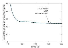
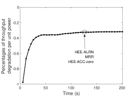
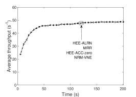
Figure 1: Performance evaluation of HEE-ACC-zero and HEE-ALRN against the timeline, where $\rho=5$.

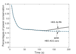
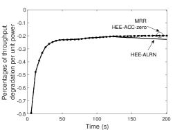
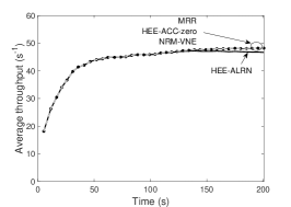
Figure 2: Performance evaluation of HEE-ACC-zero and HEE-ALRN against the timeline, where $\rho=7.5$.

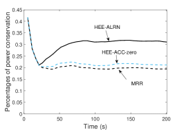
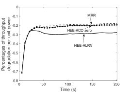
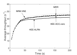
Figure 3: Performance evaluation of HEE-ACC-zero and HEE-ALRN against the timeline, where $\rho=10$.

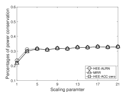
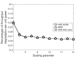
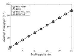
Figure 4: Performance evaluation of HEE-ACC-zero and HEE-ALRN against the scaling parameter, where $\rho=5$.

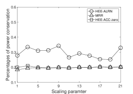
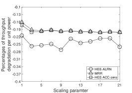
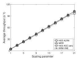
Figure 5: Performance evaluation of HEE-ACC-zero and HEE-ALRN against the scaling parameter, where $\rho=7.5$.

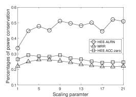
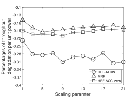
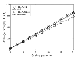
Figure 6: Performance evaluation of HEE-ACC-zero and HEE-ALRN against the scaling parameter, where $\rho=10$.

We demonstrate through simulations the effectiveness of our HEE-ACC-zero and HEE-ALRN policies by comparing them with two baseline policies. In Sections VI-A and VI-B, we explore the simulation results for scenarios with exponentially and non-exponentially, respectively, distributed lifespans of requests. In Section VI-A, we also consider time-varying real-world workloads by incorporating Google cluster traces [36, 37] in our simulations.

The $95\%$ confidence intervals of all the simulated results in this section, based on the Student t-distribution, are within $\pm 3\%$ of the observed mean.

VI-A Exponentially Distributed Lifespans

Consider a MEC network with 20 different destination areas $L=20$, 10 groups of ACs ($K=10$) installed on the edge of the Internet and an unlimited number of AC units located in the cloud. Each destination area includes a CN that serves $h\in\mathbb{N}_{+}$ wireless channels for various MTs, and is connected with the ACs in the same area through wired connections. In this context, there are $I=20h$ wireless channels, each of which is potentially shared by multiple offloading requests with capacity $N_{i}$ ($i\in[I]$) listed in Appendix A. We set the computing capacity of each AC group $C_{k}=C^{0}_{k}h$ ($k\in[K]$) where $C^{0}_{k}$ are positive integers randomly generated from $\{5,6,\ldots,10\}$.

There are four different classes of MTs ($J=4$) that keep sending requests to the MEC system. We set the arrival rates of the requests $\lambda_{j}$ ($j\in[J]$) to be $\lambda^{0}_{j}h$, where $\lambda^{0}_{j}$ is randomly generated from $[1,1.5]$. Consider the expected lifespan of a class-$j$ request by setting $\mu_{j}(i,i^{\prime},k)=\lambda_{j}/\rho$ with given parameter $\rho$. We will specify different $\rho$ in several different simulation scenarios. The specified $\lambda_{j}$ ($j\in[J]$) for the tested simulation runs are listed in Appendix A. We refer to the parameter $h\in\mathbb{N}_{+}$ as the scaling parameter, which implies the size of the MEC system and the scale of the offloading problem. When $h$ becomes large, the studied MEC model is appropriate for an urban area with a highly dense population and compatibly many MEC servers or other computing components located near mobile users.

The wireless channels between different CNs and MTs may be interfered with and become unstable due to distances, obstacles, geographical conditions, signal power, et cetera. The starting and ending channels for each MT in class $\ell$ are selected from eligible candidates with $\mu_{i,j}>0$, where the movement of the MT determines the eligibility. We provide in Appendix A the sets of eligible candidates for the starting and ending channels of the MTs in each of the four classes, as well as the remaining parameter $w_{j,k}$ for all $j\in[J]$ and $k\in[K]$. In particular, if requests in class $j$ cannot be served by ACs in group $k$, we set $w_{j,k}\rightarrow+\infty$.

In Figures 3, 3 and 3, we evaluate the performance of HEE-ACC-zero and HEE-ALRN with respect to power conservation and throughput degradation. We examine $\rho=5,7.5,10$ in the three figures, representing cases with relatively light, moderate and heavy traffic. Define $\mathcal{E}^{\phi}$ and $\mathcal{T}^{\phi}$ as the long-run average operational power consumption and the long-run average throughput of all the requests, respectively, under policy $\phi$. In this section, we consider the percentage of power conservation of a policy $\phi$ as the relative difference between $\mathcal{E}^{\text{NRM-VNE}}$ and $\mathcal{E}^{\phi}$; that is,

$$\frac{\mathcal{E}^{\text{NRM-VNE}}-\mathcal{E}^{\phi}}{\mathcal{E}^{\text{NRM-VNE}}}.$$ (27)

Similarly, consider the percentage of throughput degradation per unit power of policy $\phi$ as the relative difference between $\mathcal{T}^{\text{NRM-VNE}}/\mathcal{E}^{\text{NRM-VNE}}$ and $\mathcal{T}^{\phi}/\mathcal{E}^{\phi}$, given by

$$\frac{\mathcal{T}^{\text{NRM-VNE}}/\mathcal{E}^{\text{NRM-VNE}}-\mathcal{T}^{\phi}/\mathcal{E}^{\phi}}{\mathcal{T}^{\text{NRM-VNE}}/\mathcal{E}^{\text{NRM-VNE}}}.$$ (28)

The HEE-ACC-zero and HEE-ARLN policies proposed in this paper are compared to two baseline policies: Maximum expected Revenue Rate (MRR) [38] and Node Ranking Measurement virtual network embedding (NRM-VNE) [39]. MRR and NRM-VNE are both priority-style policies that always select the channel-AC tuple with the highest instantaneous revenue rate per unit requirement and the highest product of the AC and the channels’ remaining capacities, respectively. We adapt MRR and NRM-VNE to our MEC system by considering the wireless channels and AC units as substrate network resources used to support the incoming requests. In particular, from [38], MRR was demonstrated to be a promising policy that aims to maximize the long-run average revenue, which is equivalent to the minimization of the long-run average power consumption discussed in this paper. More precisely, for the MEC system in this paper, the instantaneous revenue per unit requirement of MRR for the tuple $(i,i^{\prime},k)$ and class-$j$ requests reduces to

$$-\frac{\lambda_{j}w_{j,k}\varepsilon_{k}}{(\lambda_{j}+\mu_{j}(i,i^{\prime},k))(w_{j,k}+2)}\mathds{1}\{k<K+1\}\\ -\frac{\lambda_{j}\mu_{j}(i,i^{\prime},k)\bar{\varepsilon}_{j}}{(\lambda_{j}+\mu_{j}(i,i^{\prime},k)(w_{j,k}+2)}\mathds{1}\{k=K+1\}.$$ (29)

The NRM-VNE was proposed in [39] to avoid traffic congestion and aimed to achieve a maximized throughput.

In Figure 3, HEE-ALRN, HEE-ACC-zero, and MRR achieve over $20\%$ conservation against NRM-VNE with respect to operational power, while the throughput of the four policies are compatible. In this case, with relatively light traffic, HEE-ALRN, HEE-ACC-zero and MRR have almost the same performance with respect to both power consumption and average throughput. When the traffic becomes heavier, in Figures 3 and 3, HEE-ALRN achieves clearly higher energy conservation than that of HEE-ACC-zero and MRR, while keeps comparable average throughput with the other three policies. HEE-ALRN, HEE-ACC-zero and MRR still maintain the $20\%$ or more power conservation against the NRM-VNE policy. We also plot Figures 3, 3 and 3 for the throughput degradation per unit power of all the four policies. Observing these figures, HEE-ALRN, HEE-ACC-zero and MRR all achieve substantially higher throughput per unit power than that of NRM-VNE. That is, there is no throughput degradation per unit power but throughput improvement per unit power when HEE-ALRN, HEE-ACC-zero or MRR is employed. It is caused by the significant power conservation but negligible throughput degradation for the three policies.

In Figures 6, 6 and 6, we examined the performance of the four policies against the scaling parameter $h$. Recall that the scaling parameter $h$ measures the size of the optimization problem. A large $h$ is appropriate for an urban area with highly dense mobile users and many compatible communication and computing capacities, which is the primary concern of this paper. Similar to Figures 3, 3 and 6, HEE-ALRN, HEE-ACC-zero and MRR in general clearly outperforms NRM-VNE in all the tested cases with respect to power consumption and throughput per unit power. The substantially higher throughput per unit power for HEE-ALRN, HEE-ACC-zero and MRR is guaranteed by their substantial power conservation with negligible degradation in average throughput. In Figures 6, 6 and 6, the performance of the policies becomes stable as the system size $h$ increases.

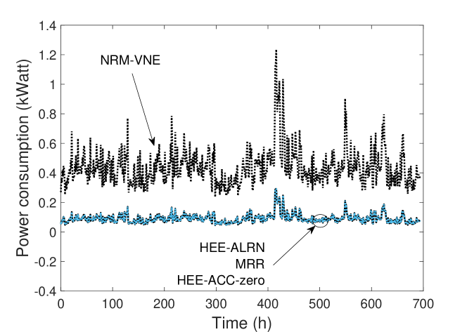
Figure 7: Average operational power consumption with Google traces.

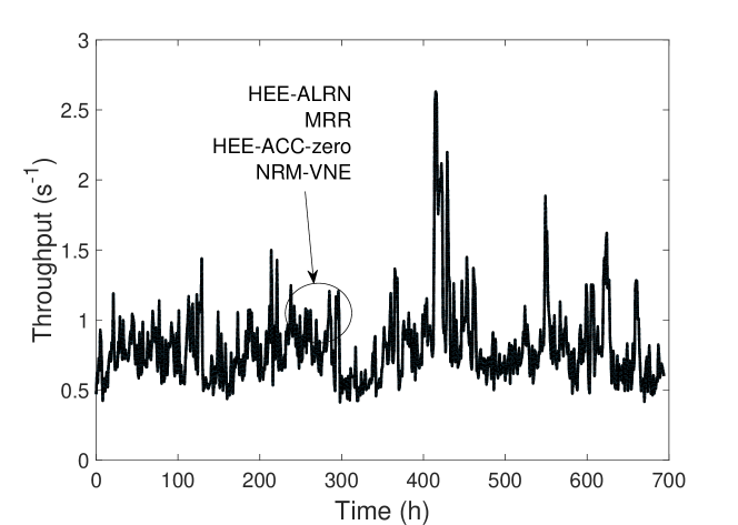
Figure 8: Average throughput with Google traces.

Apart from the time-invariant arrival rates discussed earlier in this section, we further consider time-varying arrival rates of requests. We incorporate Google cluster traces [36, 37] in the same MEC system with $\rho=10$ and $h=1$. As demonstrated in Figures 7 and 8, HEE-ALRN, HEE-ACC-zero, and MRR still achieves significantly lower power consumption while compatible throughput that NRM-VNE. As the offered traffic is relatively light, HEE-ALRN, HEE-ACC-zero, and MRR have similar performance, which is consistent with the earlier observations in Figures 3 and 6.

VI-B Non-exponential Lifespans

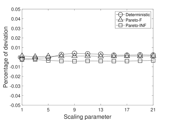
Figure 9: Deviations of average operational power consumption with non-exponentially distributed request lifespans under HEE-ACC-zero.

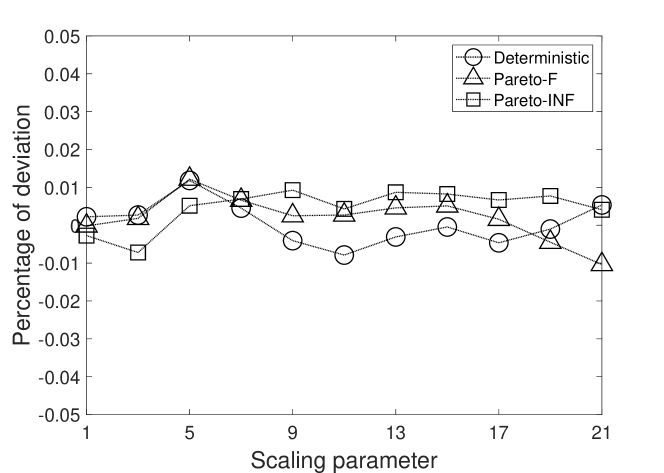
Figure 10: Deviations of average operational power consumption with non-exponentially distributed request lifespans under HEE-ALRN.

For a large-scale MEC system, the system performance is expected to be robust against different distributions of request lifespans, because, even if some sub-channels and AC units are busy to serve excessively long requests, the subsequently arrived requests are still likely to be supported by compatibly many idle sub-channels and AC units. The long-run average performance of the entire system is unlikely to be significantly affected by different shapes of the lifespan distributions, such as the heavy-tailed distributions [40, 41].

In Figures 10 and 9, we evaluate the effects of non-exponentially distributed request lifespans for HEE-ACC-zero and HEE-ALRN, respectively. Similar to the settings in [34], we simulated four different lifespan distributions for the requests: deterministic, exponential, Pareto distribution with finite variance (Pareto-F), and Pareto distribution with infinite variance (Pareto-INF). Pareto-F and Pareto-INF are constructed by setting the shape distribution of the Pareto distribution to 2.001 and 1.98, respectively. Other simulation settings are the same as those for Figures 3 and 6.

In Figures 10 and 9, the y-axis stands for the relative deviation between the power consumption for a specified lifespan and that for the exponentially distributed lifespan. That is, let $\mathcal{E}^{\phi,D}$ represent the average power consumption under the policy $\phi$ and the lifespan distribution $D$, the y-axis of Figures 10 and 9 represents

$$\frac{\mathcal{E}^{\phi,D}-\mathcal{E}^{\text{HEE-ACC-zero},\text{Exponential}}}{\mathcal{E}^{\phi,\text{Exponential}}},$$ (30)

for the policies $\phi=$HEE-ACC-zero and HEE-ALRN, respectively, with specified distributions $D=$Deterministic, Pareto-F, and Pareto-INF. In the figures, the deviations are all the time within $\pm 2\%$, which is negligible given that the confidence intervals of the simulations are considered to be $\pm 3\%$ of the means. It is consistent with the argument stated at the beginning of this subsection.

VII Conclusions

We have studied the energy efficiency of a large-scale MEC offloading problem with task handover. As mentioned earlier in the paper, the complexity and the large size of the problem prevent conventional optimization techniques from being directly applied. We have adapted the restless bandit technique to the MEC offloading problem and have proposed a class of online strategies, the HEE-ACC policies, that are applicable to realistically scaled MEC systems. If appropriate capacity coefficients are provided, then the HEE-ACC strategies achieve proved asymptotic optimality – an asymptotically optimal strategy approaches optimality as the scale of the MEC system tends to infinity. It implies that the proposed strategies are likely to be near-optimal in the practical cases with highly dense mobile users and compatibly many communication channels and computing components. We have also proposed two specific strategies within the HEE-ACC class, the HEE-ACC-zero and HEE-ALRN. The former is neat with proved asymptotic optimality in special cases and the latter is expected to achieve a higher performance by dynamically learning the most appropriate capacity coefficients. In Section VI, we have numerically demonstrated the effectiveness of HEE-ACC-zero and HEE-ALRN by comparing them with two baseline policies. It has been demonstrated that HEE-ALRN outperforms HEE-ACC-zero with respect to power conservation, which is consistent with our discussion in Section V. We have further demonstrated the robustness of the two policies, through numerical simulations, against different lifespan distributions of the proposed policies.

Appendix A Simulation Settings

In the system discussed in Section VI,

• for $i\in[I]$, the channel capacities are $N_{i}=\bar{N}_{\lfloor(i-1)/h\rfloor+1}$ where $(\bar{N}_{1},\bar{N}_{2},\ldots,\bar{N}_{10})=(8,5,5,7,6,5,5,6,5,7)$ and $(\bar{N}_{11},\bar{N}_{12},\ldots,\bar{N}_{20})=(9,6,6,5,5,9,9,9,5,7)$;

• the AC capacities are $(C_{1}^{0},C_{2}^{0},\ldots,C_{10}^{0})=(5,9,6,6,5,5,8,8,5,9)$;

• for all $k\in[K]$, the requested AC units $w_{1,k}=3$, $w_{2,k}=4$, $w_{3,k}=2$ and $w_{4,k}=1$;

• and the arrival rates of requests are $(\lambda_{1},\lambda_{2},\ldots,\lambda_{4})=(1.097,1.026,1.456,1.383)$;

All the above-listed numbers are instances generated by a pseudo-random generator in C++. Let $\mathscr{I}_{j}^{\text{start}}$ and $\mathscr{I}_{j}^{\text{end}}$ represent the sets of eligible candidates for the starting and ending channels of requests in class $j\in[J]$, respectively.

References

- [1] X. Huang, R. Yu, D. Ye, L. Shu, and S. Xie, “Efficient workload allocation and user-centric utility maximization for task scheduling in collaborative vehicular edge computing,” IEEE Transactions on Vehicular Technology, vol. 70, no. 4, pp. 3773–3787, 2021.
- [2] M. Li, J. Gao, L. Zhao, and X. Shen, “Deep reinforcement learning for collaborative edge computing in vehicular networks,” IEEE Transactions on Cognitive Communications and Networking, vol. 6, no. 4, pp. 1122–1135, 2020.
- [3] P. Dai, K. Liu, X. Wu, H. Xing, Z. Yu, and V. C. S. Lee, “A learning algorithm for real-time service in vehicular networks with mobile-edge computing,” in ICC 2019 - 2019 IEEE International Conference on Communications (ICC), 2019, pp. 1–6.
- [4] F. Busacca, C. Grasso, S. Palazzo, and G. Schembra, “A smart road side unit in a microeolic box to provide edge computing for vehicular applications,” IEEE Transactions on Green Communications and Networking, vol. 7, no. 1, pp. 194–210, 2023.
- [5] L. Li and P. Fan, “Latency and task loss probability for noma assisted mec in mobility-aware vehicular networks,” IEEE Transactions on Vehicular Technology, vol. 72, no. 5, pp. 6891–6895, 2023.
- [6] D. Lin and Y. Tang, “Edge computing-based mobile health system: Network architecture and resource allocation,” IEEE Systems Journal, vol. 14, no. 2, pp. 1716–1727, 2020.
- [7] J. Ren, Y. He, G. Huang, G. Yu, Y. Cai, and Z. Zhang, “An edge-computing based architecture for mobile augmented reality,” IEEE Network, vol. 33, no. 4, pp. 162–169, 2019.
- [8] L. Zhang and J. Chakareski, “UAV-assisted edge computing and streaming for wireless virtual reality: Analysis, algorithm design, and performance guarantees,” IEEE Transactions on Vehicular Technology, vol. 71, no. 3, pp. 3267–3275, 2022.
- [9] T. Deng, Y. Chen, G. Chen, M. Yang, and L. Du, “Task offloading based on edge collaboration in mec-enabled iov networks,” Journal of Communications and Networks, vol. 25, no. 2, pp. 197–207, 2023.
- [10] M. D. Hossain, T. Sultana, S. Akhter, M. I. Hossain, G.-W. Lee, C. S. Hong, and E.-N. Huh, “Computation offloading strategy based on multi-armed bandit learning in microservice-enabled vehicular edge computing networks,” in 2023 International Conference on Information Networking (ICOIN), 2023, pp. 769–774.
- [11] N. Monir, M. M. Toraya, A. Vladyko, A. Muthanna, M. A. Torad, F. E. A. El-Samie, and A. A. Ateya, “Seamless handover scheme for mec/sdn-based vehicular networks,” Journal of Sensor and Actuator Networks, vol. 11, no. 1, 2022.
- [12] W. Shu and Y. Li, “Joint offloading strategy based on quantum particle swarm optimization for mec-enabled vehicular networks,” Digital Communications and Networks, vol. 9, no. 1, pp. 56–66, 2023.
- [13] P. Whittle, “Restless bandits: Activity allocation in a changing world,” J. Appl. Probab., vol. 25, pp. 287–298, 1988.
- [14] J. Fu, B. Moran, and P. G. Taylor, “A restless bandit model for resource allocation, competition, and reservation,” Operations Research, vol. 70, no. 1, pp. 416–431, Mar. 2021.
- [15] A. Islam, A. Debnath, M. Ghose, and S. Chakraborty, “A survey on task offloading in multi-access edge computing,” Journal of Systems Architecture, vol. 118, p. 102225, 2021.
- [16] Z. Sun and M. R. Nakhai, “An online learning algorithm for distributed task offloading in multi-access edge computing,” IEEE Transactions on Signal Processing, vol. 68, pp. 3090–3102, 2020.
- [17] M. Zhao, J.-J. Yu, W.-T. Li, D. Liu, S. Yao, W. Feng, C. She, and T. Q. S. Quek, “Energy-aware task offloading and resource allocation for time-sensitive services in mobile edge computing systems,” IEEE Transactions on Vehicular Technology, vol. 70, no. 10, pp. 10 925–10 940, 2021.
- [18] T. Liu, D. Guo, Q. Xu, H. Gao, Y. Zhu, and Y. Yang, “Joint task offloading and dispatching for mec with rational mobile devices and edge nodes,” IEEE Transactions on Cloud Computing, pp. 1–12, 2023.
- [19] B. Xiang, J. Elias, F. Martignon, and E. D. Nitto, “Joint planning of network slicing and mobile edge computing: Models and algorithms,” IEEE Transactions on Cloud Computing, vol. 11, no. 1, pp. 620–638, 2023.
- [20] R. Xie, J. Fang, J. Yao, X. Jia, and K. Wu, “Sharing-aware task offloading of remote rendering for interactive applications in mobile edge computing,” IEEE Transactions on Cloud Computing, vol. 11, no. 1, pp. 997–1010, 2023.
- [21] P. Zhao, J. Tao, L. Kangjie, G. Zhang, and F. Gao, “Deep reinforcement learning-based joint optimization of delay and privacy in multiple-user mec systems,” IEEE Transactions on Cloud Computing, pp. 1–1, 2022.
- [22] M. Z. Alam and A. Jamalipour, “Multi-agent drl-based hungarian algorithm (madrlha) for task offloading in multi-access edge computing internet of vehicles (iovs),” IEEE Transactions on Wireless Communications, vol. 21, no. 9, pp. 7641–7652, 2022.
- [23] L. Chen, J. Wu, J. Zhang, H.-N. Dai, X. Long, and M. Yao, “Dependency-aware computation offloading for mobile edge computing with edge-cloud cooperation,” IEEE Transactions on Cloud Computing, vol. 10, no. 4, pp. 2451–2468, 2022.
- [24] Y. Lin, Y. Zhang, J. Li, F. Shu, and C. Li, “Popularity-aware online task offloading for heterogeneous vehicular edge computing using contextual clustering of bandits,” IEEE Internet of Things Journal, vol. 9, no. 7, pp. 5422–5433, 2022.
- [25] L. Gillam, K. Katsaros, M. Dianati, and A. Mouzakitis, “Exploring edges for connected and autonomous driving,” in IEEE INFOCOM 2018 - IEEE Conference on Computer Communications Workshops (INFOCOM WKSHPS), April 2018, pp. 148–153.
- [26] M. Mukherjee, L. Shu, and D. Wang, “Survey of fog computing: Fundamental, network applications, and research challenges,” IEEE Communications Surveys Tutorials, vol. 20, no. 3, pp. 1826–1857, thirdquarter 2018.
- [27] G. Lee, W. Saad, and M. Bennis, “An online secretary framework for fog network formation with minimal latency,” in 2017 IEEE International Conference on Communications (ICC), May 2017, pp. 1–6.
- [28] C. You, K. Huang, H. Chae, and B. Kim, “Energy-efficient resource allocation for mobile-edge computation offloading,” IEEE Transactions on Wireless Communications, vol. 16, no. 3, pp. 1397–1411, March 2017.
- [29] R. Deng, R. Lu, C. Lai, and T. H. Luan, “Towards power consumption-delay tradeoff by workload allocation in cloud-fog computing,” in 2015 IEEE International Conference on Communications (ICC), June 2015, pp. 3909–3914.
- [30] F. Jalali, K. Hinton, R. Ayre, T. Alpcan, and R. S. Tucker, “Fog computing may help to save energy in cloud computing,” IEEE Journal on Selected Areas in Communications, vol. 34, no. 5, pp. 1728–1739, May 2016.
- [31] J. Wu, E. W. M. Wong, Y.-C. Chan, and M. Zukerman, “Power consumption and gos tradeoff in cellular mobile networks with base station sleeping and related performance studies,” IEEE Transactions on Green Communications and Networking, vol. 4, no. 4, pp. 1024–1036, 2020.
- [32] J. C. Gittins, K. Glazebrook, and R. R. Weber, Multi-armed bandit allocation indices: 2nd edition. Wiley, Mar. 2011.
- [33] Q. Wang, J. Fu, J. Wu, B. Moran, and M. Zukerman, “Energy-efficient priority-based scheduling for wireless network slicing,” in Proc. IEEE GLOBECOM 2018, Abu Dhabi, UAE, Dec. 2018.
- [34] J. Fu and B. Moran, “Energy-efficient job-assignment policy with asymptotically guaranteed performance deviation,” IEEE/ACM Transactions on Networking, vol. 28, no. 3, pp. 1325–1338, 2020.
- [35] S. P. Boyd and L. Vandenberghe, Convex optimization. Cambridge University Press, 2004.
- [36] J. Wilkes, “More Google cluster data,” Google research blog, Nov. 2011, posted at http://googleresearch.blogspot.com/2011/11/more-google-cluster-data.html, accessed at Jul. 8, 2019.
- [37] C. Reiss, J. Wilkes, and J. L. Hellerstein, “Google cluster-usage traces: format + schema,” Google Inc., Mountain View, CA, USA, Technical Report, Nov. 2011, revised 2014-11-17 for version 2.1. Posted at https://github.com/google/cluster-data, accessed at Jul. 8, 2019.
- [38] J. Fu, B. Moran, P. G. Taylor, and C. Xing, “Resource competition in virtual network embedding,” Stochastic Models, vol. 37, no. 1, pp. 231–263, 2020.
- [39] P. Zhang, H. Yao, and Y. Liu, “Virtual network embedding based on computing, network, and storage resource constraints,” IEEE Internet of Things Journal, vol. 5, no. 5, pp. 3298–3304, 2017.
- [40] M. E. Crovella and A. Bestavros, “Self-similarity in World Wide Web traffic: evidence and possible causes,” IEEE/ACM Trans. Netw., vol. 5, no. 6, pp. 835–846, Dec. 1997.
- [41] M. Harchol-Balter, Performance Modeling and Design of Computer Systems: Queueing Theory in Action. Cambridge University Press, 2013.