Automatic Truss Design with Reinforcement Learning

Abstract

Truss layout design, namely finding a lightweight truss layout satisfying all the physical constraints, is a fundamental problem in the building industry. Generating the optimal layout is a challenging combinatorial optimization problem, which can be extremely expensive to solve by exhaustive search. Directly applying end-to-end reinforcement learning (RL) methods to truss layout design is infeasible either, since only a tiny portion of the entire layout space is valid under the physical constraints, leading to particularly sparse rewards for RL training. In this paper, we develop AutoTruss, a two-stage framework to efficiently generate both lightweight and valid truss layouts. AutoTruss first adopts Monte Carlo tree search to discover a diverse collection of valid layouts. Then RL is applied to iteratively refine the valid solutions. We conduct experiments and ablation studies in popular truss layout design test cases in both 2D and 3D settings. AutoTruss outperforms the best-reported layouts by 25.1% in the most challenging 3D test cases, resulting in the first effective deep-RL-based approach in the truss layout design literature.

1 Introduction

Truss layout design and optimization is a crucial and fundamental research topic in the building industry, as truss layouts can be found in a wide range of structures, including bridges, towers, roofs, floors Stolpe (2016); Alhaddad et al. (2020) and even in aerospace and automotive sectors Wang et al. (2019). As a basic component in building structures, a truss can support heavy loads and span long distances with a small amount of construction material. Efficient truss layout design can lead to significant cost savings and can also improve the physical performance and safety of the structure.

However, truss layout design is an NP-hard combinatorial optimization problem, which involves the optimization of node locations, topology between nodes, and the cross-sectional areas of connecting bars Fenton et al. (2015). The possible search space for truss layouts is huge, nonlinear, and non-convex. There are also a number of constraints that must be satisfied, including material strength, displacement allowance, and stability of structural members Luo et al. (2022b). Traditionally, engineers design and optimize truss layouts using a combination of mathematical analysis and physical testing based on domain knowledge. They analyze the structural behavior and iteratively adjust the size and shape based on initial sketches Dorn (1964). These methods rely heavily on subjective human expertise, resulting in a cumbersome and restrictive design process. An automated design approach is crucial for achieving greater efficiency and flexibility in the design process.

Previous studies have attempted to automate the design of truss layouts using heuristic algorithms, such as genetic algorithms Permyakov et al. (2006), particle swarm optimization Luh and Lin (2011), simulated annealing Lamberti (2008), and differential evolutionHo-Huu et al. (2016). However, the size and the complexity of the search space impeded the achievement of optimal results. Note that the entire search space, including node positions, is continuous, and a tiny position change may drastically influence the physical performance of the entire truss layout. So, directly applying search-based methods can be particularly expensive. A low-resolution discretization over the search space may easily miss out on the optimal positions and lead to low-quality solutions Luo et al. (2022b).

Reinforcement learning (RL) methods have achieved strong results in solving combinatorial optimization problems Mazyavkina et al. (2021), such as the Traveling Salesman Problem (TSP) Bello et al. (2016) and drug design Jeon and Kim (2020); Yoshimori et al. (2020). These problems require the solver to find the optimal combination of a finite set of choices to maximize a certain objective function. Truss layout design is a similar combinatorial problem but it has the following differences. Unlike TSP problems where any order of the cities is feasible, truss layout design and optimization have tight physical constraints, making most truss layouts generated from random actions invalid. This in turn makes reward signals sparse for RL training. The objective function is also more complex than that in TSP, since there are more performance indices, like capacity and stability, beyond total mass. The settings of truss layout design are more similar to virtual screening in drug design, namely identifying potential drug candidates from large libraries of compounds Yoshimori et al. (2020). They both have complex constraints and performance indices. However, in drug design, there exists a large amount of data that can be used for pre-training Jeon and Kim (2020), whereas in truss layout design, little real-world data are available. These facts make it difficult to directly apply end-to-end RL training to truss layout design.

To sum up, the heuristic search methods can generate valid truss layouts, but with sub-optimal quality Luo et al. (2022b). On the other hand, RL can produce fine-grained refinement of truss layouts but suffer from sparse rewards. Therefore, we combine them as a two-stage search-and-refine algorithm named AutoTruss. In the search stage, we run a search-based method, Upper Confidence bounds applied to Trees (UCT), to derive diverse truss layouts under all physical constraints. In the refinement stage, we adopt the SAC algorithm to train an RL policy for refining the valid truss layouts from the search stage. We conduct experiments in both 2D and 3D cases, and results show that AutoTruss improved the SOTA performance by $6.8\%$ on average in 2D test cases and as much as $25.1\%$ in the more challenging 3D test cases.

2 Related Work

2.1 Truss Representation

A concise representation of a truss layout is fundamental for the truss layout design, which should capture both geometry and load conditions. There are mainly two types of representations: voxel-based Li et al. (2022), and graph-based Stolpe (2016). We adopt the graph-based method for its accuracy and flexibility. The voxel-based methods divide the design space into small, three-dimensional units called voxels, each assigned a value representing material density Li et al. (2022); Klemmt (2023); Du et al. (2018). These methods cope well with boundary conditions, but cannot accommodate continuous variations in truss topology and is prone to discretization errors.

On the other hand, graph-based methods represent the truss layout as a graph, consisting of coordinates of nodes, bars connecting the nodes, and member area sizes Fenton et al. (2015); Stolpe (2016); Lieu (2022), but often simplifying it to follow certain grids or only connecting neighboring nodes. Based on a graph-based approach, our method adopts a continuous additive method, allowing for greater flexibility in node connection and truss layout by adding nodes and connections freely from scratch. Furthermore, Graph Neural Network (GNN) Scarselli et al. (2008) is well-suited for processing graph-structured data and complex relationships between elements, thus it is widely used in various real-world applications such as social networks Li et al. (2021), chemistry Fung et al. (2021); Yang et al. (2021), and recommendation systems Guo and Wang (2020); Wu et al. (2019a).

2.2 Truss Design and Optimization

There have been various methods for truss layout design and optimization over the years. Traditionally, engineers designed truss layouts based on sketches by experience and refined them with analytical math tools Dorn (1964). This empirical method is time-consuming and far from accurate. With the advancement of technology, computer algorithms based on finite element analysis (FEA) have been adopted for faster and more efficient design Mai et al. (2021). These algorithms can be divided into two categories: gradient-based and non-gradient-based. Gradient-based algorithms, such as steepest descent, are efficient in converging to a solution but can be complex to implement mathematically and often produces local solutions Banh et al. (2021); Nguyen and Banh (2018); Banh and Lee (2019); Lieu (2022). On the other hand, non-gradient-based algorithms, such as differential evolution (DE) and genetic algorithms (GA), do not require derivative calculations and are more flexible and robust in the presence of multiple local optima. As a relatively new entrant in this category, Monte Carlo Tree Search (MCTS) Coulom (2007) has shown to be highly effective in large search spaces with the success of AlphaGo Silver et al. (2016), as it balances exploration and exploitation Luo et al. (2022b, a). Different from previous works which simultaneously optimize truss topology and member sizes, we implement a two-stage search-and-refine approach to sequentially optimize topology and member sizes, which greatly reduces the search space and thus improves the training speed as well as the accuracy of the results. In this paper, we adopt UCT Kocsis and Szepesvári (2006), a variant of MCTS, as the search method for deriving various valid truss layouts in the search stage.

2.3 RL for Combinatorial Optimization

Recently, reinforcement learning (RL) has emerged as a powerful tool for solving challenging combinatorial optimization problems, such as virtual screening in drug design Wu et al. (2019b); Deudon et al. (2018). Various RL algorithms have been applied in this field, including value-based methods like Q-learning Khalil et al. (2017), policy-based methods Bello et al. (2016) and policy-gradient based methods Kool et al. (2018). One representative method in RL is Soft Actor-Critic (SAC) Haarnoja et al. (2018), which has been used in robotics Taylor et al. (2021), autonomous vehicles Guan et al. (2022), game playing Zhou et al. (2022) and many others. In this study, we also leverage the power of RL to address a combinatorial optimization problem, which is fine-grain truss refinement. Specifically, we employ SAC algorithm for this task, as it has a high sample efficiency and a strong ability to explore the solution space.

3 Preliminary

3.1 Problem Formulation

The truss layout design task is to minimize the mass of a truss layout by defining node locations, connections between the nodes, and cross-sectional areas of bars. Formally, a truss layout can be represented as a graph $G=(V,E)$, where $V$ is the set of nodes and $E$ is the set of bars. A bar $e\in E$ can be defined as a tuple $e=(u,v,z)$, with nodes $u,v\in V$, and cross-sectional area $z\in\mathbb{R}$. The mass can be written as

$$\text{ Mass }(G)=\sum_{(u,v,z)\in E}z\times\left\|u-v\right\|$$ (1)

In truss layout design, certain physical constraints need to be satisfied, to ensure displacement, stress, and buckle condition are within capacity, while the length, area, and slenderness of the bars are within the design limit. Constraint details can be found in Appendix A.1. We consider both 2D and 3D settings in this paper. The only difference is the calculation of the bar’s cross-sectional area. In 2D settings, the cross-sectional area is only decided by the width of the bar. While in 3D settings, each bar is a hollow round tube, and the cross-sectional area is decided by the outer diameter and its thickness.

3.2 Upper Confidence Bounds Applied to Trees

Upper confidence bounds applied to trees (UCT) algorithm Kocsis and Szepesvári (2006) modifies Monte Carlo tree search (MCTS) method with Upper Confidence bounds, which searches for the best termination state $s^{*}$ with the highest reward $R_{UCT}(s^{*})$ with a balance between exploration and exploitation Gelly and Silver (2007). Classical UCT is applied to finite states and actions. For each non-termination state $s$, UCT maintains an action-value function $Q(s,a)$ during tree search, which is calculated as Equ. (2):

$$Q(s,a)=\beta W_{\text{mean}}(s,a)+(1-\beta)W_{\text{best}}(s,a),$$ (2)

where $W_{\text{mean}}$ denotes the average reward of all the termination states in the subtree rooted at state $s$, and $W_{\text{best}}$ represents the highest reward in the subtree. $\beta$ is a hyper-parameter to control the exploration preference between the average and the best reward Kocsis and Szepesvári (2006).

The policy of UCT $\pi_{UCT}(s)$ selects the action that maximizes the upper confidence bound on the action value by

$$Q_{UCT}(s,a) =Q(s,a)+c\sqrt{\dfrac{\log n(s)}{n(s,a)}};$$ (3)

$$\pi_{UCT}(s) =\text{argmax}_{a}Q_{UCT}(s,a),$$ (4)

where $n(s)$ is the number of times that state $s$ has been visited, and $n(s,a)$ is the number of times that action $a$ has been taken from state $s$. Whenever a state $s$ is visited, the counter $n(s)$ and $n(s,a)$ will be increased by 1.

When UCT begins, all the action values will be initialized to 0. In each UCT iteration, the search process starts from the root state $s_{0}$ and expands the search tree according to Equ. (4). Simulation will be executed till a termination state is reached. Then the counters and the action values of visited state-action pairs will be updated accordingly. The process will be repeated within a given budget of search steps.

3.3 Reinforcement Learning

Reinforcement learning (RL) trains an agent to learn to make decisions by interacting with an environment and receiving feedback in the form of rewards. The agent’s goal is to maximize its total reward over time. To apply RL training, we model the problem as a Markov Decision Process (MDP). MDP is parameterized by $\langle S,A,R,P,\gamma\rangle$, where $S$ is the state space, $A$ is the action space, $R$ is the reward function, $P\left(s^{\prime}\mid s,a\right)$ is the transition probability from state $s$ to state $s^{\prime}$ via action $a$, and $\gamma$ is the discount factor. The goal is to find a policy $\pi_{\theta}$ parameterized by $\theta$ that outputs an action $\pi_{\theta}(s)\in A$ for each state $s$ and maximizes the accumulative expected reward. The objective function is shown in Equ. (5).

$$J(\theta)=\mathbb{E}_{a_{t}\sim\pi_{\theta}(s_{t})}\left[\sum_{t}\gamma^{t}R\left(s_{t},a_{t}\right)\right]$$ (5)

3.3.1 Soft Actor-Critic

Soft Actor-Critic (SAC) is an off-policy reinforcement learning algorithm that combines the actor-critic framework with an entropy term to encourage exploration. SAC optimizes

$$J(\pi)=\mathbb{E}_{\pi}\left[\sum_{t}R(s_{t},a_{t})+\alpha\cdot H\left(\pi(s_{t})\right)\right],$$ (6)

where $H\left(\pi\right)$ is the entropy of the policy at state $s_{t}$, and $\alpha$ is a temperature coefficient balancing exploration and exploitation. SAC maintains a data buffer $D$ with all the transition samples and learns a soft Q-function $Q_{\psi}(s,a)$ parameterized by $\psi$. Assuming the policy is parameterized by $\theta$, SAC optimizes the policy by the following objective

$$J(\theta)=\mathbb{E}_{s_{t}\sim D}\left[\mathbb{E}_{a_{t}\sim\pi_{\theta}(s_{t})}\left[\alpha\log\pi_{\theta}(a_{t}|s_{t})-Q_{\psi}(s_{t},a_{t})\right]\right].$$ (7)

The temperature $\alpha$ and the parameter $\psi$ of the soft Q-network are also learned similarly.

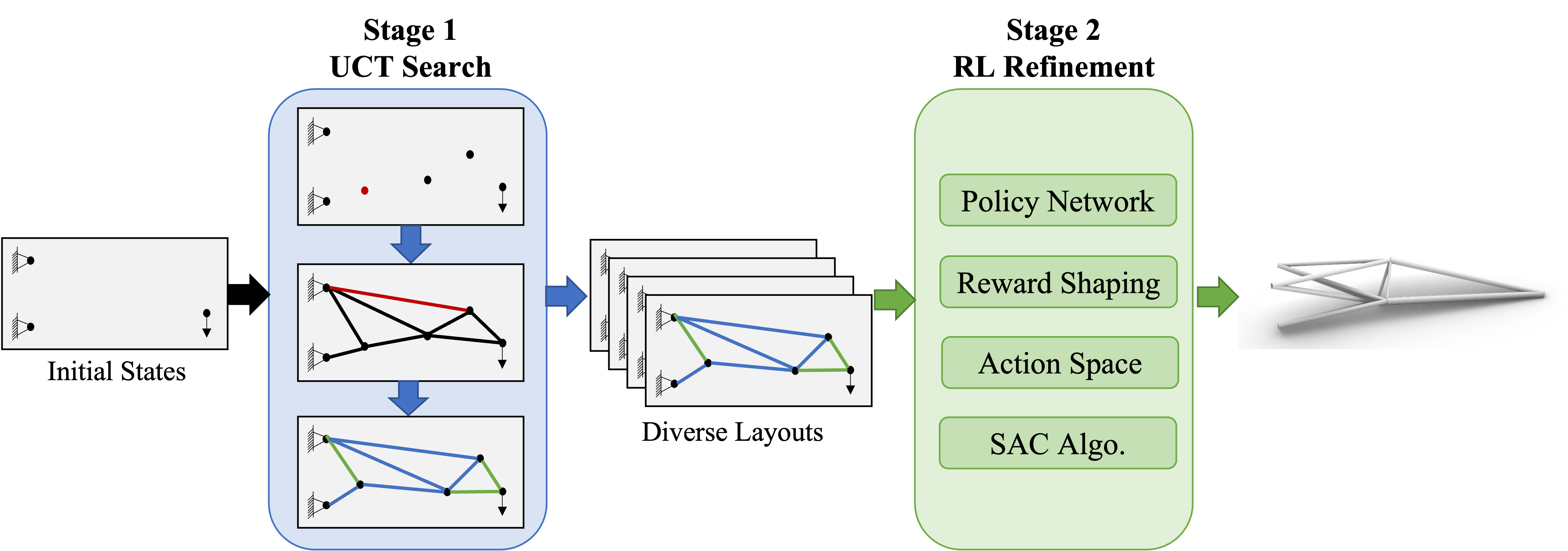
Figure 1: Overview of the two-stage approach AutoTruss. In the search stage, UCT Search is applied for diverse valid truss layouts. In the refinement stage, we adopt SAC algorithm to train a policy for truss layout refinement.

4 AutoTruss: A Two-Stage Method

Truss layout design has a huge search space, which makes it extremely expensive for exhaustive search methods to achieve high performance. It is not feasible to apply end-to-end reinforcement learning (RL) methods either, since there are many restrictions on valid truss layouts, yielding highly sparse reward signals. Therefore, we proposed AutoTruss, a two-stage method consisting of a search stage and a refinement stage. In the search stage, AutoTruss uses a UCT search for diverse valid layouts. In the refinement stage, AutoTruss adopts deep RL to further improve the valid solutions. The overview of AutoTruss is shown in Fig. 1 with details described below.

4.1 Search Stage: UCT for Valid Designs

The purpose of the search stage is to find diverse valid truss layouts as a foundation for the refinement stage. We remark that diversity is important since similar topologies from the search stage will yield similar results from the refinement stage, while diverse inputs for the RL policy will improve the overall performances and robustness of AutoTruss.

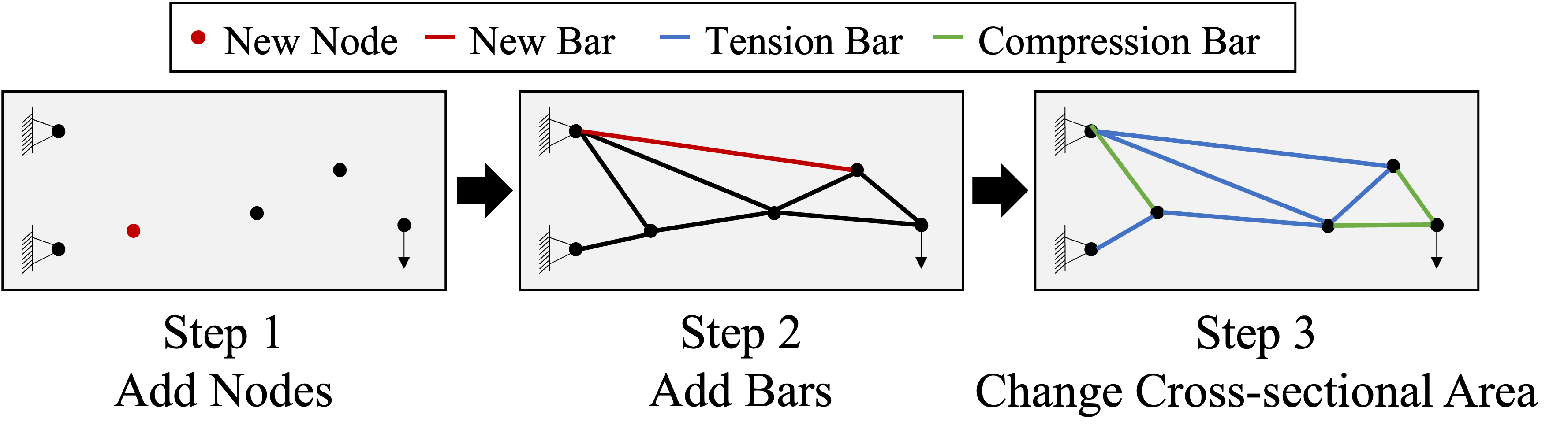
Figure 2: Pipeline of UCT search. UCT search sequentially adds nodes, adds bars, and changes bar cross-sectional area.

We use UCT search to find valid truss layouts. We divide the generation process of a truss layout into three steps: node-adding step, bar-adding step, and cross-sectional area-changing step. The pipeline of UCT search is shown in Fig. 2. To be specific, given the initial truss layout $G_{0}=(V_{0},E_{0})$, our UCT search takes these three steps sequentially to produce a complete layout $G_{m}=(V_{m},E_{m})$ from scratch. In the node-adding step, it adds new nodes to the layout until it reaches the maximum number of nodes, and then in the bar-adding step, bars with a random cross-sectional area will be added to the truss layout until it satisfies the structural constraints described in Sec. 3.1. Finally, we choose the appropriate cross-sectional area for each added bar in the cross-sectional area changing step. Following Luo et al. (2022b), for each complete truss layout $G_{m}=(V_{m},E_{m})$, the reward is defined by

$$R_{UCT}(G_{m})=\left\{\begin{array}[]{cl}-1~{}~{},&\text{invalid (structural);}\\ 0~{}~{},&\text{invalid (other);}\\ \dfrac{\kappa}{\text{ Mass }(G_{m})^{2}},&\text{valid layout,}\end{array}\right..$$ (8)

$\kappa$ is a scaling parameter, which is typically chosen to bound the maximum reward below 10 for numerical stability.

4.1.1 UCT Search with Continuous Actions

A challenge when applying classical UCT to truss layout design is that the actions are all continuous. Therefore, for any intermediate truss layout $G$, finding the optimal UCT action $\pi_{UCT}(G)$ according to Equ. (4) becomes non-trivial. In AutoTruss, we approximate the best action by drawing random samples and choosing the optimal action from the samples:

$$\hat{a}_{(i)}\sim \text{Uniform}(A)\quad\forall 1\leq i\leq N,$$

$$\hat{\pi}_{UCT}(G)= \arg\max_{a=\hat{a}_{(1)},\ldots,\hat{a}_{(N)}}Q_{UCT}(G,a).$$ (9)

In our implementation, we choose $N=25$.

Another issue for continuous actions is to compute the action value $Q_{UCT}(G,a)$ since there are infinitely many such values to compute leading to an unbounded search tree size. In our implementation, we constrained the expansion size for each intermediate truss layout $G$ such that we at most expand $O(\sqrt{n(G)})$ children to compute the exact values Yee et al. (2016). For other state-action pair $(G,a^{\prime})$ without tree expansion, we approximate its $Q(G,a^{\prime})$ and $n(G,a^{\prime})$ via kernel regression Nadaraya (1964) based on the precise values of the expanded actions from $G$. Suppose there are $M$ expanded actions, i.e., $\bar{a}_{(1)},\ldots,\bar{a}_{(M)}$. The value $Q(G,a^{\prime})$ can be approximated by

$$\hat{Q}(G,a^{\prime})=\frac{\sum_{i=1}^{M}K(a^{\prime},\bar{a}_{(i)})n(G,\bar{a}_{(i)})Q(G,\bar{a}_{(i)})}{\sum_{i=1}^{M}K(a^{\prime},\bar{a}_{(i)})n(G,\bar{a}_{(i)})}.$$ (10)

The counts $n(G,a^{\prime})$ can be similarly approximated. Here $K(.,.)$ denotes a kernel function. We simply adopt the Gaussian kernel in our implementation.

4.1.2 Diverse Layouts

To get diverse valid truss layouts for the refinement stage, we not only need to save the best truss layout, but also some other suboptimal valid truss layouts. Note that two truss layouts $G_{1},G_{2}$ are topologically the same if and only if there exists a permutation $\sigma$ over node indices such that

$$\forall(u,v)\in G_{1},(\sigma(u),\sigma(v))\in G_{2}.$$ (11)

It is time-consuming to enumerate all the permutations, we relax the criterion and only adopt the identity permutation in practice for topology checking. Finally, we store the top 5 lightest valid layouts for each topology and use $\mathcal{G}$ to denote this set of diverse truss layouts we obtained.

4.2 Refinement Stage: RL for Adjustment

In the refinement stage, we adopt the SAC algorithm to refine those valid truss layouts $\mathcal{G}$ generated in the search stage.

4.2.1 Action Space

The RL policy needs to perform two types of actions, i.e., adjust a node position and the cross-sectional areas of a specific bar in a truss layout. For node position refinement, when given a specific node to change, the policy outputs a multi-dimensional vector denoting the change of node coordinates. In the 2-dimensional case, the policy outputs $(\delta_{x},\delta_{y})$ indicating the change in the node’s position. Similarly, in the 3-dimensional case, the policy outputs $(\delta_{x},\delta_{y},\delta_{z})$. Here all $\delta_{i}<0.5$ such that the adjustment will be confined to a small zone with dimension no more than $0.5$m. This is to ensure that the majority of actions taken by RL will not violate the constraints. For cross-sectional area changes, when given a specific bar to adjust, the policy outputs a single real value for area change in the 2-dimensional case. In the 3-dimensional case, the policy outputs two continuous actions, namely changing the outer diameter and changing the thickness of the bar. Note that not all cross-sectional areas are valid in the 3-dimensional case, so the actual values are rounded up to the minimum legal value during execution.

4.2.2 Reward Function

The design principle of the reward function is to (1) penalize invalid layouts and (2) promote lighter layouts. Suppose an action $a$ is taken on an intermediate layout $G$ leading to a refined layout $G^{\prime}$, the reward function is defined as

$$R(G,a)=\left\{\begin{array}[]{rl}-50~{}~{}~{}~{}~{}~{},&\text{invalid (structural);}\\ -10~{}~{}~{}~{}~{}~{},&\text{invalid (other);}\\ \dfrac{\kappa}{\textrm{Mass}(G^{\prime})^{2}}-\dfrac{\kappa}{\textrm{Mass}(G)^{2}},&\text{valid.}\end{array}\right..$$ (12)

4.2.3 Network Architecture

The network architecture of the RL policy is shown in Fig. 3. Inspired by the transformer architecture Vaswani et al. (2017), we adopt (1) a self-attention encoder to extract the spatial relationship between nodes and bars, and (2) an action decoder to output high-precision refinement actions for the node or bar to be operated on in the current iteration. The nodes are represented using coordinates, loads, and whether or not they are supported. The bars are represented as the coordinates of the two end nodes, with (a) the cross-sectional area of the bar in 2D, or with (b) the outer diameter and the thickness of the bar in 3D. All the nodes and bars are passed through an embedding layer and then sent to the self-attention encoder for spatial relationship extraction. The node-bar adjacency matrix is also fed into a self-attention encoder to reflect the topology of the truss layout. Then, the results of the embedding layer for the node or bar being operated in the current iteration will be sent to the action decoder together with its embedding of the self-attention encoder. Finally, the policy outputs both the Q values and the multi-dimensional action. Full details can be found in Appendix A.4.

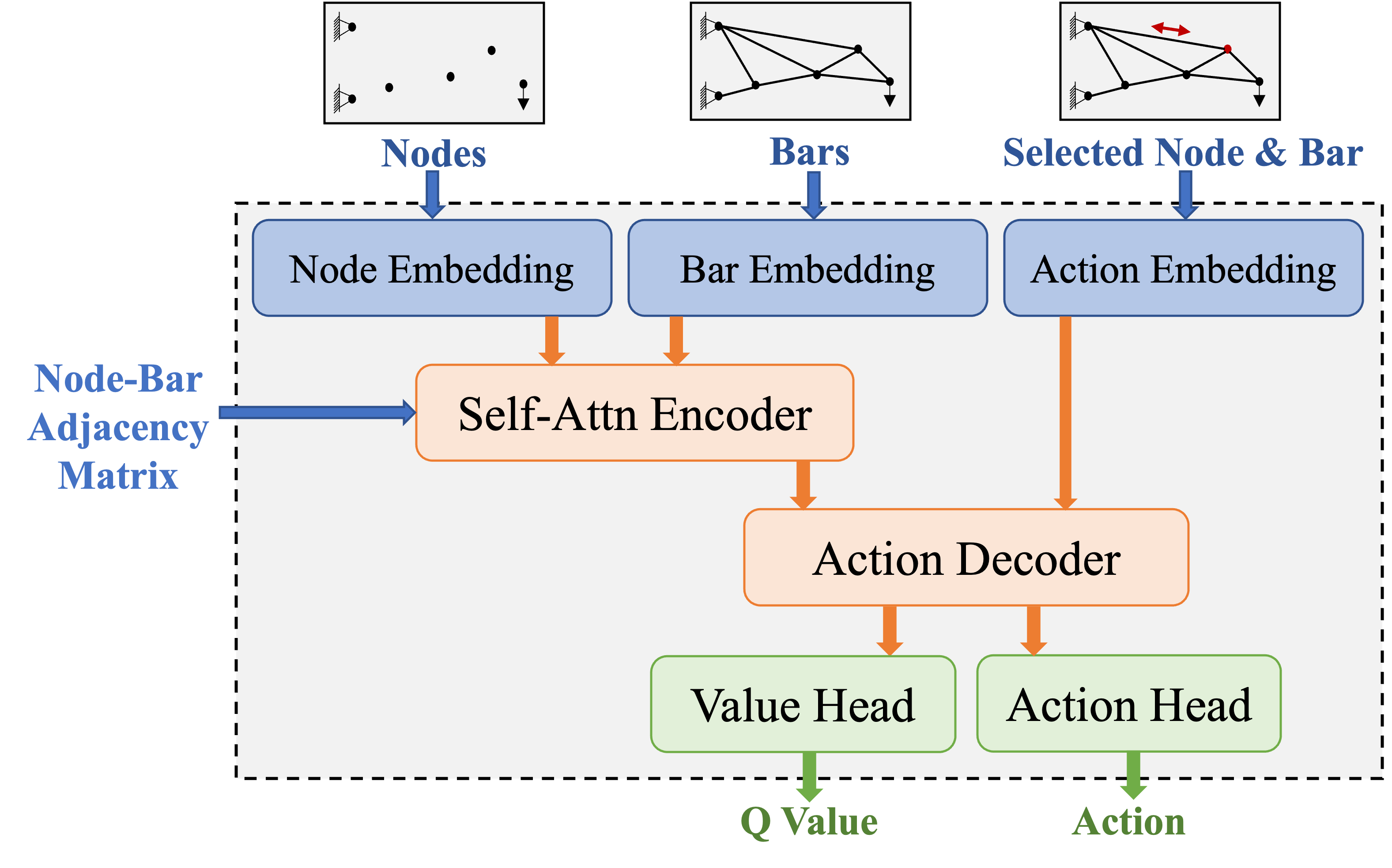
Figure 3: Network architecture of RL policy in the refinement stage.

4.2.4 Rollout Generation for RL Training

In our approach, we employ a probabilistic initialization strategy for the initial state of RL. In particular, we keep maintaining the top-5 diverse layouts in $\mathcal{G}$. When each episode starts, we uniformly sample from $\mathcal{G}$ with 50% probability. Otherwise, we alternatively start from the top-5 lightest truss layouts found during training without considering topology diversity. The termination criterion of one episode is that the maximum number of 20 actions are performed. We also early terminate an episode if the policy generates 5 invalid layouts within a single episode. In addition, in each RL step, we randomly choose a node or a bar from the current layout for the policy to adjust. More details can be found in Appendix A.5.

4.3 Overall Algorithm

We summarize the overall process of AutoTruss in Algorithm 1. The input to the algorithm is the initial truss layout $G_{0}=(V_{0},E_{0})$ as well as the constraints. $V_{0}$ represents the support nodes and $E_{0}$ represents the fixed bars. After applying the two stages, the algorithm finally outputs the lightest truss layout ever derived during the entire search process.

Algorithm 1 AutoTruss

1:Initial truss layout $G_{0}=(V_{0},E_{0})$, where $V_{0}$ means fixed node set and $E_{0}$ means the fixed bar set.

2:Diverse Truss Set $\mathcal{G}\leftarrow\emptyset$

3:while Tree Search Steps $<$ Limit do $\triangleright$ search stage

4:     Search from $(V_{0},E_{0})$ w.r.t. Equ. (9)

5:     Update counts and value for expanded nodes

6:     Update $\mathcal{G}$

7:end while

8:Initialize the policy $\pi$, data buffer $D$ $\triangleright$ refinement stage

9:while RL steps $<$ RL Limit do

10:     Select initial state from $\mathcal{G}$

11:     Generate an episode $\tau$ w.r.t. the policy $\pi_{\theta}$

12:     Update $\mathcal{G}$

13:     Add $\tau$ to D and update $\pi_{\theta}$ via SAC

14:end while

15:return $\arg\min_{G\in\mathcal{G}}\textrm{Mass}(G)$

5 Experiments

We compare AutoTruss with 3 search-based baselines using both 2D and 3D test cases, where AutoTruss consistently produces the best truss designs. We also evaluate the effectiveness of each module in AutoTruss through ablation studies. We introduce test cases in Sec. 5.1, baselines in Sec. 5.2, and the experiment setup in Sec. 5.3. Main results and ablation studies are in Sec. 5.4 and Sec. 5.5 respectively.

5.1 Testbeds

5.1.1 2D Testbed

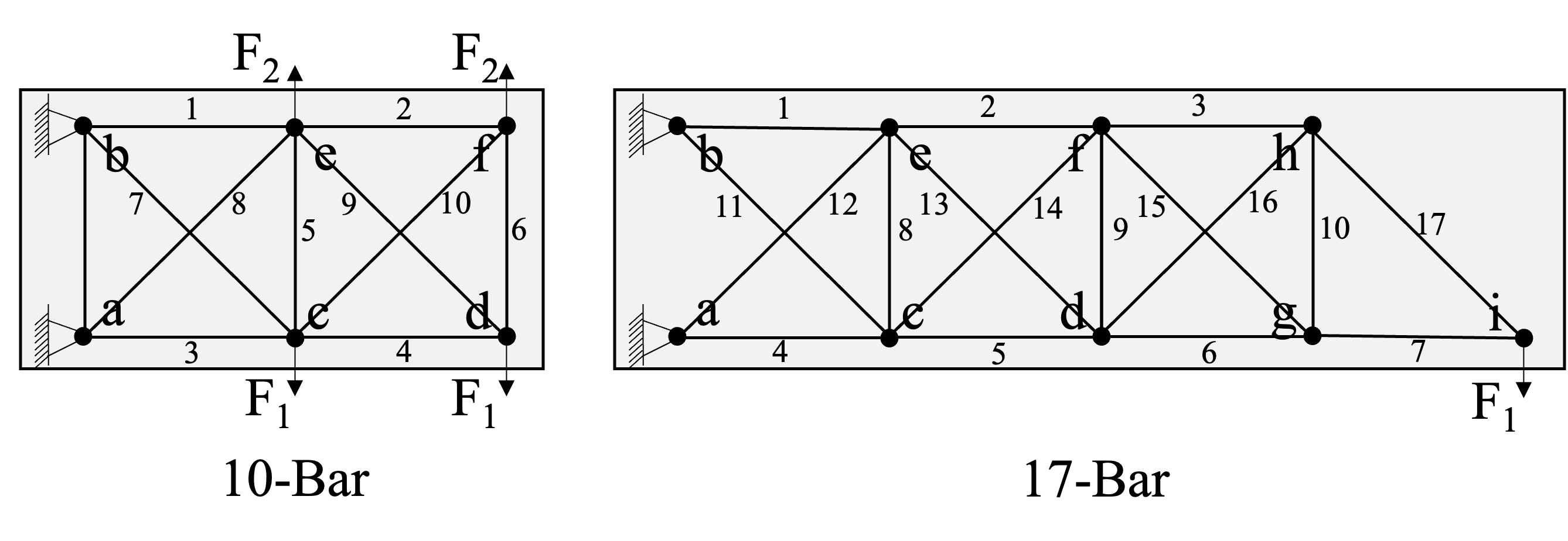
Figure 4: 10-Bar and 17-Bar truss layout design cases of the 2D testbed. In the 10-Bar case, there are $2$ kinds of load cases. Load case I has four fixed nodes $(a,b,c,d)$, whereas load case II has six fixed nodes $(a,b,c,d,e,f)$. In the 17-Bar case, there are $3$ fixed nodes $(a,b,i)$. In all 2D cases, $(a,b)$ are support nodes.

We choose two common 2D test cases in truss layout design Fenton et al. (2015): the 10-Bar Cantilever Truss (10-Bar) and the 17-Bar Cantilever Truss (17-Bar), as shown in Fig.4. Both are common test cases in the field of structure generation and optimization Assimi et al. (2017); Deb and Gulati (2001); Tejani et al. (2018); Fenton et al. (2015) . There are $2$ load cases in the 10-Bar case. The buckle constraint and the slenderness constraint are not applied to the 10-Bar case. In the 17-Bar case, all the constraints except the slenderness constraint are taken into consideration. The detailed settings are listed in Appendix A.1.

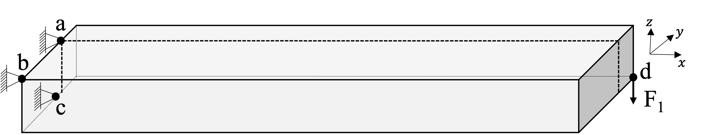
Figure 5: Cantilever Sundial truss layout design case of the 3D testbed. There are $4$ fixed nodes $(a,b,c,d)$. $(a,b,c)$ are support nodes.

5.1.2 3D Testbed

We select the Cantilever Sundial Design (Sundial) as the 3D testbed, which follows Luo et al. (2022a). The test case was adapted from the sundial bracket truss located in Paternoster Square, London, UK Shea and Zhao (2004). As shown in Fig. 5, the Sundial testbed is characterized by a higher dimension and a larger scale and complexity of the solution space when compared to the 2D testbed.

5.2 Baselines

We consider 3 competitors: AlphaTruss Luo et al. (2022b), KR-UCT Luo et al. (2022a), and SEOIGE Fenton et al. (2015). All the baseline methods can be applied to the 2D testbed, but only KR-UCT can be applied to the 3D testbed. Therefore, we compare 2D results with all three baselines and compare 3D results only with KR-UCT. We utilized the results of the baselines as reported in their original papers, as the test cases and evaluation methods used in those studies were consistent with those employed in our own research. The details of baselines are listed in Appendix A.2.

5.3 Experiment Setup

KR-UCT and SEOIGE use single-stage search while we use a two-stage search scheme. We balance the iterations in the search stage, and the environment steps in the refinement stage to keep a fair comparison. More specifically, we run $2e6$ iterations in the search stage, which is half the number of iterations in KR-UCT, and $1.5e5$ environment steps for RL training, so that the running time of the refinement stage is similar to the search stage with an RTX 3070 GPU. We remark that AutoTruss consumes substantially fewer trials (i.e., search iterations + RL steps) compared with baselines, and The details can be found in Appendix A.8. We run $3$ seeds for each test case and report the best numbers with the mean numbers and standard deviations.

5.4 Main Results

5.4.1 2D Results

The mass of the solutions derived by AutoTruss and baselines are presented in Tab. 1, where $p$ denotes the number of nodes in truss layouts. AutoTruss outperforms the baselines in all the settings by an average of $6.8\%$, demonstrating its ability to discover more lightweight truss layouts. Moreover, The illustration of the truss layouts is shown in Fig. 6. AutoTruss find the same truss layout topology with better refinement in 10-Bar load I case, and finds better topologies in other cases.

Cases	Settings	AlphaTruss	KR-UCT	SEOIGE	AutoTruss
10-Bar	Load I, $p$=6	2150	2154	2218	2114(2128, 17.6)
	Load II, $p$=7	1616	N/A	2098	1337(1410, 61.2)
17-Bar	$p$=6	1408	1463	2582	1378(1398, 22.2)

Table 1: Results of 10-Bar and 17-Bar truss layout design in 2D testbed. $p$ is the number of nodes in the generated truss layouts. N/A denotes that the original paper does not report the number. AutoTruss outperforms baselines in all cases, showing the capacity to generate lighter truss layouts under various settings.

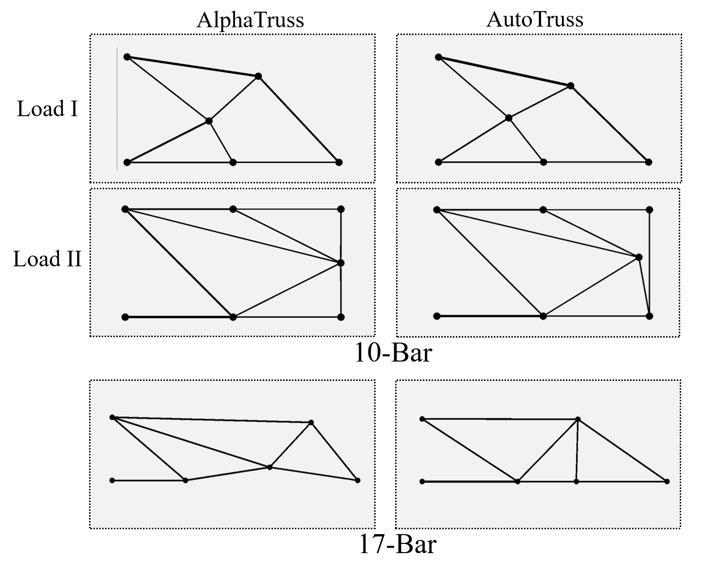
Figure 6: Visualization of truss layouts derived by AutoTruss and AlphaTruss in 2D testbed. We demonstrate 10-Bar truss layouts under 2 settings and the 17-Bar truss layout. The thicker lines represent larger cross-sectional areas. AutoTruss derives the same truss layout topology as AlphaTruss but with better refinement in 10-Bar load I case, and derives better topologies in other cases. The pictures of AlphaTruss are adopted from the original paper.

5.4.2 3D Results

Tab. 2 shows a comparison of AutoTruss and KR-UCT in the Cantilever Sundial truss layout design of the 3D testbed. Our method consistently outperforms KR-UCT by at least $25\%$ under all settings. This highlights the effectiveness of AutoTruss in designing lightweight truss layouts within a larger search space. It is noteworthy that 3D truss design poses a greater challenge than 2D truss design, as the search space is substantially enlarged. Our approach exhibits a more significant improvement in the 3D case than the 2D counterpart.

The visualization comparison is shown in Fig. 7. The truss layouts derived by AutoTruss show a more elongated appearance compared with those derived by KR-UCT.

Settings	KR-UCT	AutoTruss
$p$ = 7	N/A	30.6(31.3, 0.63)
$p$ = 8	38.7	29.0(30.4, 1.01)
$p$ = 9	37.2	28.8(30.5, 1.32)

Table 2: Results of Cantilever Sundial truss layout design in 3D testbed. $p$ is the number of nodes in the generated truss layouts. N/A denotes the original paper does not report the number. AutoTruss outperforms KR-UCT by $25.1\%$, showing the ability to generate complex 3D truss layouts.

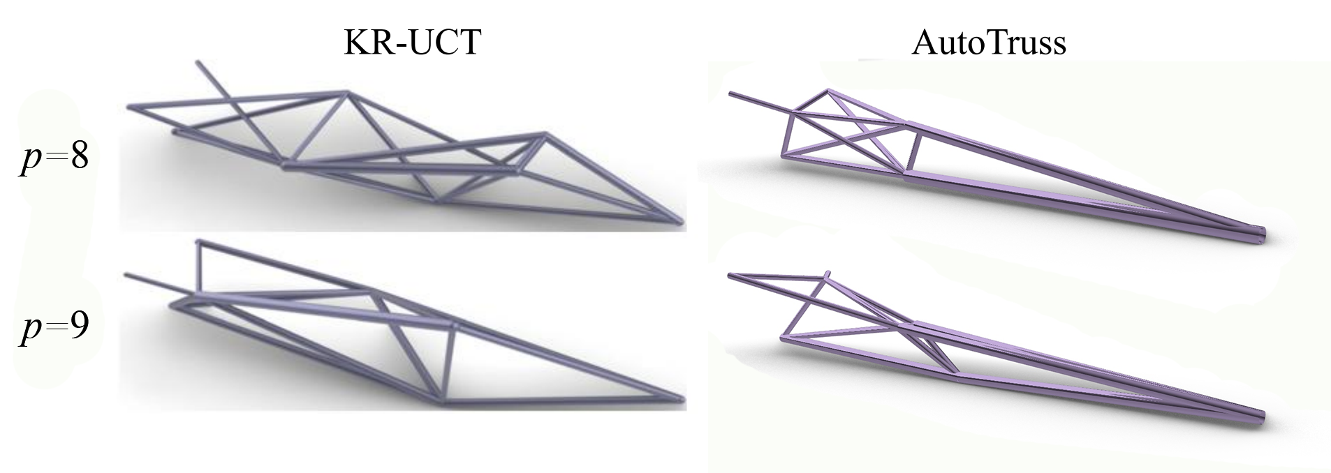
Figure 7: Visualization of truss layouts derived by AutoTruss and KR-UCT in 3D testbed. $p$ is the number of nodes in the generated truss layouts. The truss layouts derived by AutoTruss are more slender and streamlined than those derived by KR-UCT.

.

5.5 Ablation Study

In this section, we analyze the effectiveness of the two-stage scheme, the usage of diverse truss layouts in the search stage, as well as network architecture, all based on the 10-Bar truss layout design cases of 2D testbed through ablation studies. Results are reported as “mean (standard deviation)”.

5.5.1 Search-Stage-Only v.s. Two-Stage

We present truss layouts only derived from the search stage and refined by the refinement stage separately in Fig. 8. In all cases, the refinement stage substantially reduces the total mass of the truss layout by $28\%$ on average, demonstrating the importance of the refinement stage in AutoTruss for further performance improvement.

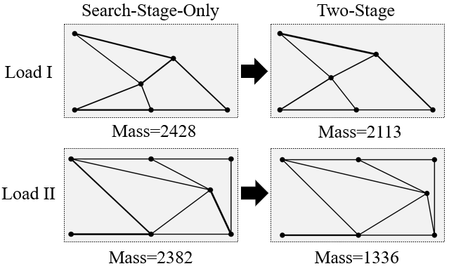
Figure 8: Comparison of truss layouts only derived by the search stage (Search-Stage-Only) and refined by the refinement stage(Two-Stage). The refinement stage can effectively tune truss layouts in both node positions and bar cross-sectional areas.

5.5.2 Usage of Diverse Truss Layouts

To investigate the advantages of the diverse truss layouts derived in the search stage, we use the lightest truss layouts derived in the search stage without different topologies, named AutoTruss w.o. Diverse. The results are presented in Tab. 3. AutoTruss outperforms AutoTruss w.o. Diverse by an average of $3\%$ in all cases, which demonstrates the effectiveness of introducing diverse truss layouts.

Settings	AutoTruss w.o. Diverse	AutoTruss
Load I, $p$ = 6	2149.60(1.90)	2128.73(17.83)
Load II, $p$ = 7	1419.67(18.45)	1410.73(61.17)

Table 3: Ablation studies on the usage of diverse truss layouts. AutoTruss w.o. Diverse directly uses the lightest truss layouts derived in the search stage without different topologies. AutoTruss achieves better performance under all settings.

5.5.3 Network Architecture

Transformer and GNN architectures are commonly employed to handle graphical inputs. The comparison between GNN-based Policy and AutoTruss is presented in Tab. 4. We utilized CGConv Fey and Lenssen (2019) as GNN module, which has been demonstrated to exhibit good performance in material property prediction tasks Xie and Grossman (2018). The node positions, loads, and support information are embedded as nodes, and the cross-sectional area of each bar is recorded as an edge property. After GNN, we extract the embedding of the action node and then concatenate it with the action embedding for the final action. Empirically, we observe that a Transformer-based policy, as we used in AutoTruss, performs slightly better than a GNN-based Policy.

Settings	GNN-based Policy	AutoTruss
Load I, $p$ = 6	2151.64(12.10)	2128.73(17.83)
Load II, $p$ = 7	1412.93(99.87)	1410.73(61.17)

Table 4: Ablation studies on the network architecture. AutoTruss, which adopts Transformer-based architecture, shows slightly better performance than GNN-based Policy.

6 Conclusion

We propose a two-stage method AutoTruss that can automatically design truss layouts under various constraints. We use UCT search to find diverse valid truss layouts in the search stage and then use deep RL policy to refine the truss layouts derived in the search stage. AutoTruss outperforms the baselines by $6.8\%$ on 2D testbed and $25.1\%$ on 3D testbed. AutoTruss may perform poorly when generating large-scale spatial structures, and combining basic structural elements in the search stage could accelerate the search speed. We leave this as our future work.

Contribution Statement

Authors Weihua Du and Jinglun Zhao contributed equally to this work and should be considered co-first authors.

Appendix A Appendix

A.1 Detailed Constraints

For any truss layout $G=(V,E)$, we have $8$ constraints in total to check whether the truss layout is valid.

We define some parameters first: $\Omega$ is the design domain, $z_{i}$ is the cross-sectional area of $i$-th bar, $l_{i}$ is the length of $i$-th bar, $\sigma_{i}$ is the stress of $i$-th bar ($\sigma_{i}>0$ means the bar is in tension and $<0$ means in compression), $\delta_{i}$ is the displacement of $i$-th nodes from its original position after loaded, $\sigma_{i}^{c}=\max(0,-\sigma_{i})$ is the compression part of stress, $b_{i}=\pi^{2}EI_{i}/z_{i}l_{i}^{2}$ refers to the buckling limit of $i$-th bar ($E$ is Young’s modulus, $I_{i}$ is the moment of inertia of $i$-th bar), $\lambda_{i}=l_{i}/\sqrt{I_{i}/z_{i}}$ is the slenderness ratio of $i$-th bar.

The $8$ constraints $g_{0},...,g_{8}$ are listed as following:

• Geometry stability$(g_{0})$: the truss layout must pass three basic checks: (a) no extra degree of freedom, (b) stiffness matrix $\succ 0$, (c) no intersection between bars;

• Design domain$(g_{1})$: each node and bar should be in the design domain $\Omega$;

• Cross-sectional area$(g_{2})$: each bar’s cross-sectional area $z_{i}$ should be within $[z_{\min},z_{\max}]$;

• Stress constraint$(g_{3})$: each bar’s strength $\sigma_{i}$ should be within $[\sigma_{\min},\sigma_{\max}]$;

• Displacement$(g_{4})$: each node’s displacement $\delta_{i}$ should be within a small range in each direction. i.e, $\|\delta_{i}\|_{\infty}\leq\delta_{\max}$;

• Stability$(g_{5})$: each bar’s compression part of stress $\sigma_{i}^{c}$ should be less than its buckle limit $b_{i}$.

• Stiffness$(g_{6})$: each bar’s slenderness ratio $\lambda_{i}$ should be less than $\lambda_{\max}$;

• Bar length$(g_{7})$: each bar’s length $l_{i}$ should be within $[l_{\min},l_{\max}]$.

Notice that not all the constraints need to be satisfied in the test cases, and some test cases take the self-weight into consideration. We specify the constraint set in each test case in A.2.

A.2 Detailed Settings of Testbeds

A.2.1 10-Bar Cantilever Truss

The design domain of the 10-Bar Cantilever Truss is shown in Fig. 4 left. The 10-Bar Truss test case has $6$ fixed nodes. The left two nodes $(a,b)$ are support nodes, and the right four nodes $(c,d,e,f)$ may take some loads. The test case has two load cases. Load case I only has loads on nodes $(c,d)$, while Load case II has loads on all the four nodes $(c,d,e,f)$. If a fixed node has no load and is not a support node, it will be removed from the initial truss layout. Constraints $\{g_{0},g_{1},g_{2},g_{3},g_{4}\}$ need to be satisfied in the 10-Bar test case. The node numbers $p$ of load case I and II are $6$ and $7$, respectively. This test case does not take the self-weight of bars into consideration.

Detailed information on fixed nodes is listed in Tab. 5. Material properties and constraint parameter settings are listed in Tab. 6.

Node	Location(mm)	Load Case 1	Load Case 2
a	(0, 0)	Support	Support
b	(0, 9144)	Support	Support
c	(9144, 0)	Loaded (0, -444,800 N)	Loaded (0, -667,200 N)
d	(18288, 0)	Loaded (0, -444,800 N)	Loaded (0, -667,200 N)
e	(9144, 9144)	N/A	Loaded (0, 444,800 N)
f	(18288, 9144)	N/A	Loaded (0, 444,800 N)

Table 5: Each fixed node information of the 10-Bar test case.

Parameters	Values
Design Domain$(\Omega)$	$[0,18,288]\times[0,9,144]$ mm
Young’s modulus$(E)$	$68,950\text{ MPa}(10,000\text{ ksi})$
Density$(\rho)$	$2767.99\text{ kg/m}^{3}(0.1\text{ lb/in}^{3})$
Stress range$(\sigma_{\min},\sigma_{\max})$	$[-172.369,172.369]\text{ MPa}([-25,25]\text{ksi})$
Max node displacement$(\delta_{\max})$	$50.8\text{ mm}(2\text{ in})$
Bar area range$(z_{\min},z_{\max})$	$[0.6452,225.806]\text{ cm}^{2}$
Consider self-weight$(f_{self})$	No

Table 6: Detailed constant information of the 10-Bar test case.

A.2.2 17-Bar Cantilever Truss

The design domain of the 17-Bar Cantilever Truss is shown in Fig. 4 right. The 17-Bar Truss test case has $3$ fixed nodes. The left two nodes $(a,b)$ are support nodes, and node $(i)$ takes some loads. Constraints $\{g_{0},g_{1},g_{2},g_{3},g_{4},g_{5}\}$ need to be satisfied in the 17-Bar test case. The node number $p$ is $6$. This test case does not take the self-weight of bars into consideration.

Detailed information on fixed nodes is listed in Tab. 7. Material properties and constraint parameter settings are listed in Tab. 8.

Node	Location(mm)	Load
a	(0.0, 0.0)	Support
b	(0.0, 2540.0)	Support
i	(10160.0, 0.0)	Loaded (0, -444,800 N)

Table 7: Each fixed node information of the 17-Bar test case.

Parameters	Values
Design Domain$(\Omega)$	$[0,10,160]\times[0,2,540]$ mm
Young’s modulus$(E)$	$206,850\text{ MPa}(30,000\text{ ksi})$
Density$(\rho)$	$7418.21\text{ kg/m}^{3}(0.268\text{ lb/in}^{3})$
Stress range$(\sigma_{\min},\sigma_{\max})$	$[-334.6,334.6]\text{ MPa}([-50,50]\text{ksi})$
Max node displacement$(\delta_{\max})$	$50.8\text{ mm}(2\text{ in.})$
Bar area range$(z_{\min},z_{\max})$	$[0.6452,225.806]\text{ cm}^{2}$
Consider self-weight$(f_{self})$	No

Table 8: Detailed constant information of the 17-Bar test case.

A.2.3 3D Cantilever Sundial

The design domain of the 3D Cantilever Sundial test case is shown in Fig. 5. The design domain only represents node locations and there is no mandatory geometric boundary for newly added nodes and bars. There are four fixed nodes in the design domain, among which nodes $(1,2,3)$ are support nodes, and node $(4)$ is the sundial tip with load $50$ N. Constraints $\{g_{0},g_{1},g_{2},g_{3},g_{4},g_{6},g_{7}\}$ need to be satisfied in the Sundial test case. The node number $p$ is $7$ or $8$ or $9$. This test case takes the self-weight of bars into consideration.

Detailed information on fixed nodes is listed in Tab. 9. Material properties and constraint parameter settings are listed in Tab. 10. Note that the slenderness ratio limit is different for tension bars and compression bars ($220$ for tension bars and $180$ for compression bars).

The cross-section of the bars used in this section is the section of cold-formed thin-wall welded round steel tube (GB50018-2002)GB50018 [2002]. There are $61$ kinds of cross-sections in total and each area $z$ of the cross-sections is defined by diameter $d$ and thickness $t$: $z=\pi(d^{2}/4+(d-2t)^{2}/4)$, with parameters ranging from $d~{}25~{}t~{}1.5$ to $d~{}245~{}t~{}4.0$.

Node	Location(mm)	Load
a	(0.0, 0.0, 0.0)	Support
b	(0.0, -483, 595)	Support
c	(0.0, 483, 595)	Support
d	(4634, 772, -78)	Loaded (0, 0, -50 N)

Table 9: Each fixed node information of the 3D Sundial test case.

Parameters	Values
Design Domain$(\Omega)$	No mandatory geometric boundary
Young’s modulus$(E)$	$193\text{ GPa}$
Density$(\rho)$	$8000\text{ kg/m}^{3}(0.268\text{ lb/in}^{3})$
Strength range	$[-123,123]\text{ MPa}$
Max node displacement$(\delta_{\max})$	$2\text{ mm}$
Slenderness ratio$(\lambda_{\max})$	$220$(tension bar) and $180$(compression bar)
Bar length range$(l_{\min},l_{\max})$	$[0.03,5]$ m
Bar area range $(z)$	Cross-sections in GB50018-2002
Consider self-weight$(f_{self})$	Yes

Table 10: Detailed constant information of the 3D Sundial test case.

A.3 Detailed Baseline Description

A.3.1 AlphaTruss

AlphaTrussLuo et al. [2022b] is a two-stage search method. The first stage is searching in discrete space by UCT search. Similar to AutoTruss, it searches for node position, node connection, and cross-sectional area of bars sequentially. The second stage is used to refine the best truss layouts generated in the first stage by discretized UCT search, too. In detail, suppose $w$ is the step size of the discretization in the first stage and $p$ is the search result of a node’s position or a bar’s cross-sectional area. The search domain will be restricted to $[p-w/2,p+w/2]$.

A.3.2 KR-UCT

KR-UCTLuo et al. [2022a] is a one-stage search method, which uses UCT search directly. To handle the continuous search space, it applies the kernel method. Similarly to AlphaTruss, it searches node position, node connection, and cross-sectional area of bars sequentially. To the best of our knowledge, it is the first search method that can apply to 3D settings without any predefined structure.

A.3.3 SEOIGE

SEOIGEFenton et al. [2015] uses grammatical evolution to represent a variable number of nodes and positions on a continuum, and then uses the Delaunay triangulation algorithm to build bars between nodes. SEOIGE works well in test cases where the structure of the solution is not known a priori.

A.4 Network Architecture

All in all, the network architecture of the RL policy for AutoTruss has four parts: node/bar/action id/action embedding, self-attention encoder, action decoder, and action/value head.

A.4.1 Node/Bar/Action id/Action Embedding

For a truss layout $G=(V,E)$, AutoTruss first embeds each node $v_{i}$ and bar $e_{i}$ by MLPs. In detail, a node $v_{i}$ is represented by [position, support condition, load condition] and put into a two-layer MLP with hidden dim $128$ and output dim $256$. Similarly, a bar $e_{i}$ is represented by [node position 1, node position 2, cross-sectional area] and put into a two-layer MLP with the same hidden dim and output dim as node embedding. For the action id and action, we also use two two-layer MLPs with the same hidden dim and output dim. Let the embedded nodes, bars, action id, and action be $\hat{v_{1}},...,\hat{v_{|V|}}$, $\hat{e_{1}},...,\hat{e_{|E|}}$, $\hat{id}$, and $\hat{a}$, respectively.

A.4.2 Self-Attention Encoder

To get the connection between nodes, bars, and action id of a truss layout. We use a self-attention encoder to extract information. First, we concatenate the embedding of nodes and bars as a sequence $[\hat{v_{1}},...,\hat{v_{|V|}},\hat{e_{1}},...,\hat{e_{|E|}}]$, and then put the sequence into the self-attention encoder. The self-attention encoder has hidden dim $256$ and $6$ layers.

A.4.3 Action Decoder

To get the predicted action $a$ and the Q value $Q(s,a)$. Action id $\hat{id}$ and action $\hat{a}$ are put into the action decoder, which is a $6$ layer decoder with hidden dim $256$. Let the hidden state of action id and action generated by action decoder be $h_{id}$ and $h_{a}$, respectively.

A.4.4 Action/Value Head

We use the hidden state of action id $h_{id}$ and action $h_{a}$ to generate action $a$ and predict Q-value $Q(s,a)$, respectively. To generate action $a$, we put $h_{id}$ into a three-layer MLP with hidden dims $256,512$. Similarly, to predict Q-value $Q(s,a)$, we put $h_{a}$ into another MLP with the same hidden dims.

A.5 Hyperparameters

There are $6$ hyperparameters in our algorithm, namely the first exploration parameter $\beta$ in Equ. (2), the second exploration parameter $c$ in Equ. (3), discount factor $\gamma$ in Equ. (5), temperature parameter $\alpha$ in Equ. (6), and the learning rate of policy and Q-value function $lr_{policy}$ and $lr_{Qf}$. . The values of the hyperparameters are chosen through trial and error, with their values listed in Tab. 11.

Hyperparameters	Values
Exploration parameter I$(\beta)$	$0.3$
Exploration parameter II$(c)$	$30$
Discount factor$(\gamma)$	$0.99$
Initial temperature$(\alpha)$	$1.0$
Policy learning rate$(lr_{policy})$	$0.0003$
Q-value learning rate$(lr_{Qf})$	$0.0003$

Table 11: Hyperparameters used in UCT, RL, and SAC.

A.6 Data of Generated Truss Layouts

Detailed data of the generated truss layouts, including node coordinates and cross-sectional areas of the bars are provided in tables. Tab. 12 shows the details for both load case I and II for the 10-bar test case with illustration in Fig. 9. Tab. 13 shows the details for the 17-bar test case with illustration in Fig. 10. Tab. 14 and Tab. 15 show the details for the 3D test case.

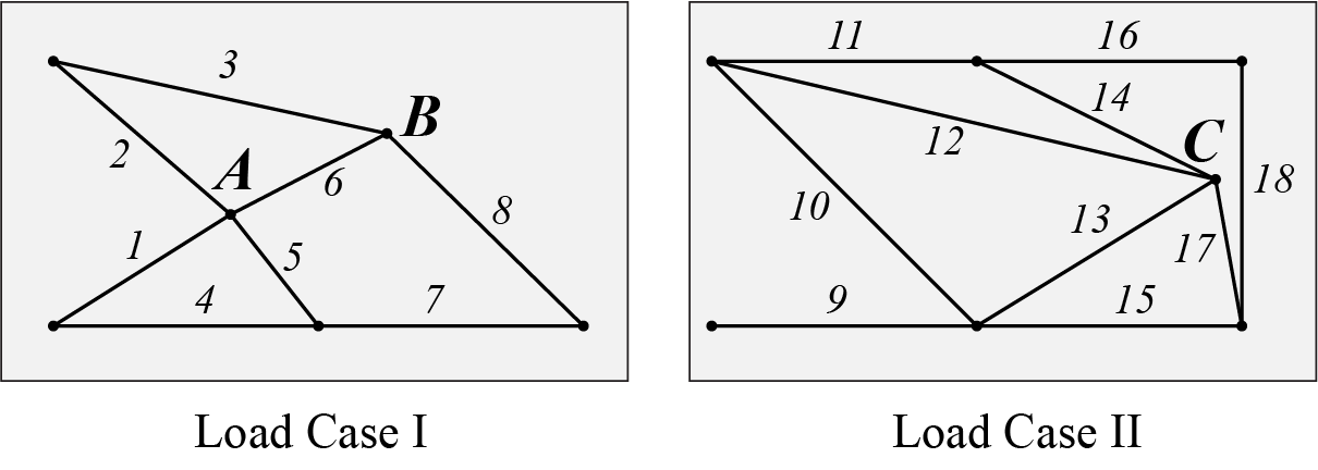
Figure 9: Illustration for the generated truss in 2D 10-bar.

.

Node Label	A		B		C
Coord. (mm)	(6115,3851)		(11508,6647)		(17380,5062)
	1	2	3	4	5	6
	125	31.8	126	189	33.2	117
Bar Label	7	8	9	10	11	12
Area (cm2)	97.9	140	165	88.7	53.6	1.06
	13	14	15	16	17	18
	58.4	57.0	14.0	0.65	63.1	12.9

Table 12: Detailed data of the generated truss in 2D 10-bar.

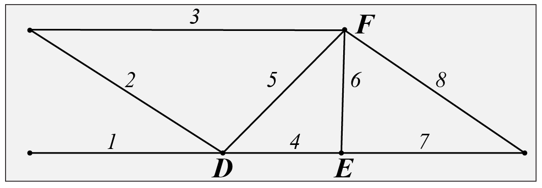
Figure 10: Illustration for the generated truss in 2D 17-bar.

.

Node Label	D			E		F
Coord. (mm)	(3963,0)			(6395,0)		(6462,2528)
Bar Label	1	2	3	4	5	6	7	8
Area (cm2)	132	38.6	47.6	48.7	71.4	0.65	76.1	41.4

Table 13: Detailed data of the generated truss in 2D 17 bar.

	3D Case Node Coordinates (m)
#	7-Point	8-Point	9-Point
1	(0, 0, 0)	(0, 0, 0)	(0, 0, 0)
2	(0, -0.48, 0.6)	(0, -0.48, 0.6)	(0, -0.48, 0.6)
3	(0, 0.48, 0.6)	(0, 0.48, 0.6)	(0, 0.48, 0.6)
4	(1.66, 0.24, -0.11)	(4.63, 0.77, -0.08)	(4.63, 0.77, -0.08)
5	(1.69, 0.3, 0.18)	(1.67, 0.31, -0.03)	(2.29, 0.38, -0.12)
6	(1.64, 0.22, 0.27)	(1.77, 0.37, 0.34)	(1.57, 0.27, 0.22)
7	(4.63, 0.77, -0.08)	(0.43, -0.08, 0.43)	(0.6, 0.14, 0.57)
8		(1.72, 0.29, 0.38)	(1.74, 0.36, 0.24)
9			(1.71, 0.23, 0.22)

Table 14: Node coordinates detail of the generated truss in 3D.

Bar Connection, Outer Diameter(mm)
(Thickness=1.5 mm, if not stated otherwise)
7-Point		8-Point		9-Point
1-5: 30.0	3-5: 25.0	1-5: 30.0	3-5: 25.0	4-9: 40.0	1-4: 40.0
1-6: 30.0	3-6: 25.0	3-6: 25.0	4-6: 40.0	3-5: 25.0	4-5: 25.0
4-6: 40.0	5-6: 25.0	5-6: 25.0	1-7: 25.0	1-6: 25.0	2-6: 25.0
1-7: 30.0	2-7: 25.0	2-7: 25.0	3-7: 25.0	3-6: 25.0	7-9: 40.0
3-7: 25.0	5-7: 25.0	5-7: 25.0	1-8: 30.0	1-7: 25.0	4-7: 25.0
6-7: 25.0		3-8: 25.0	4-8: 40.0	5-7: 25.0	6-7: 25.0
4-5: 51.0 $\leftarrow$ 2mm thick		6-8: 25.0	7-8: 25.0	8-9: 40.0	1-8: 25.0
4-7: 51.0 $\leftarrow$ 2mm thick		4-7: 51.0 $\leftarrow$ 2mm thick		3-8: 30.0	4-8: 25.0
				5-8: 25.0	6-8: 25.0
				7-8: 25.0

Table 15: Bar connections, outer diameter and thickness of the generated truss in 3D.

A.7 Ablation Study on Environment

To check the design of the RL environment, we conduct an ablation study on whether the environment allows invalid truss layouts during rollout. Under our current design, the environment allows the policy generates invalid truss layouts in less than $5$ steps within a single episode. Another environment design does not allow the policy generates any invalid layouts, and it will stop the episode immediately if any invalid layout occurs, named AutoTruss w.o Invalid. We run the ablation study on the 10-Bar test case for $3$ seeds, and the comparison is shown in Tab. 16. Data is reported as "mean(standard deviation)". Allowing the occurrence of invalid truss layouts achieves better results since it encourages the RL policy to explore more.

Settings	AutoTruss w.o. Invalid	AutoTruss
Load I, $p$ = 6	2136.01(14.91)	2128.73(17.83)
Load II, $p$ = 7	1631.41(128.69)	1410.73(61.17)

Table 16: Ablation studies on whether the environment allows invalid truss layouts. AutoTruss w.o. Invalid does not allow any invalid truss layouts to occur in the rollout. AutoTruss achieves better performance under all settings.

A.8 Comparison of Running Time

The parameters for the number of episodes used in the UCT search and the number of environment steps used in the reinforcement learning were chosen to ensure a fair comparison to other baselines, by keeping a similar time cost.

Our first baseline, KR-UCT, uses a single stage of searching with an upper limit of $4$ million iterations when running the 3d kr-sundial test case. In contrast, since our algorithm has two stages, we set the upper limit of the search stage to $2$ million iterations to keep the search time half that of KR-UCT. $150,000$ environment steps ensure that the refinement stage takes the same time as the search stage.

The second baseline, AlphaTruss, also has two stages, and its search stage takes approximately half the number of iterations as KR-UCT. Therefore, the computation for our search stage is consistent with AlphaTruss.

We report the number from their paper for the third baseline SEOIGE since its codebase is not public.

References

- Alhaddad et al. [2020] Wael Alhaddad, Yahia Halabi, Hu Xu, and HongGang Lei. Outrigger and belt-truss system design for high-rise buildings: A comprehensive review part ii—guideline for optimum topology and size design. Advances in Civil Engineering, 2020, 2020.
- Assimi et al. [2017] Hirad Assimi, Ali Jamali, and Nader Nariman-Zadeh. Sizing and topology optimization of truss structures using genetic programming. Swarm and evolutionary computation, 37:90–103, 2017.
- Banh and Lee [2019] Thanh T Banh and Dongkyu Lee. Topology optimization of multi-directional variable thickness thin plate with multiple materials. Structural and Multidisciplinary Optimization, 59(5):1503–1520, 2019.
- Banh et al. [2021] Thanh T Banh, Nam G Luu, and Dongkyu Lee. A non-homogeneous multi-material topology optimization approach for functionally graded structures with cracks. Composite Structures, 273:114230, 2021.
- Bello et al. [2016] Irwan Bello, Hieu Pham, Quoc V Le, Mohammad Norouzi, and Samy Bengio. Neural combinatorial optimization with reinforcement learning. arXiv preprint arXiv:1611.09940, 2016.
- Coulom [2007] Rémi Coulom. Efficient selectivity and backup operators in monte-carlo tree search. In International conference on computers and games, pages 72–83. Springer, 2007.
- Deb and Gulati [2001] Kalyanmoy Deb and Surendra Gulati. Design of truss-structures for minimum weight using genetic algorithms. Finite elements in analysis and design, 37(5):447–465, 2001.
- Deudon et al. [2018] Michel Deudon, Pierre Cournut, Alexandre Lacoste, Yossiri Adulyasak, and Louis-Martin Rousseau. Learning heuristics for the tsp by policy gradient. In International conference on the integration of constraint programming, artificial intelligence, and operations research, pages 170–181. Springer, 2018.
- Dorn [1964] W Dorn. Automatic design of optimal structures. J. de Mecanique, 3:25–52, 1964.
- Du et al. [2018] Tao Du, Jeevana Priya Inala, Yewen Pu, Andrew Spielberg, Adriana Schulz, Daniela Rus, Armando Solar-Lezama, and Wojciech Matusik. Inversecsg: Automatic conversion of 3d models to csg trees. ACM Transactions on Graphics (TOG), 37(6):1–16, 2018.
- Fenton et al. [2015] Michael Fenton, Ciaran McNally, Jonathan Byrne, Erik Hemberg, James McDermott, and Michael O’Neill. Discrete planar truss optimization by node position variation using grammatical evolution. IEEE Transactions on Evolutionary Computation, 20(4):577–589, 2015.
- Fey and Lenssen [2019] Matthias Fey and Jan E. Lenssen. Fast graph representation learning with PyTorch Geometric. In ICLR Workshop on Representation Learning on Graphs and Manifolds, 2019.
- Fung et al. [2021] Victor Fung, Jiaxin Zhang, Eric Juarez, and Bobby G Sumpter. Benchmarking graph neural networks for materials chemistry. npj Computational Materials, 7(1):1–8, 2021.
- GB50018 [2002] Chinese Standard GB50018. Technical code of cold-formed thin-wall steel structures. General Administration of Quality Supervision Inspection and Quarantine: Beijing, China, 2002.
- Gelly and Silver [2007] Sylvain Gelly and David Silver. Combining online and offline knowledge in uct. In ICML, 2007.
- Guan et al. [2022] Jiayi Guan, Guang Chen, Jin Huang, Zhijun Li, Lu Xiong, Jing Hou, and Alois Knoll. A discrete soft actor-critic decision-making strategy with sample filter for freeway autonomous driving. IEEE Transactions on Vehicular Technology, 2022.
- Guo and Wang [2020] Zhiwei Guo and Heng Wang. A deep graph neural network-based mechanism for social recommendations. IEEE Transactions on Industrial Informatics, 17(4):2776–2783, 2020.
- Haarnoja et al. [2018] Tuomas Haarnoja, Aurick Zhou, Pieter Abbeel, and Sergey Levine. Soft actor-critic: Off-policy maximum entropy deep reinforcement learning with a stochastic actor. In ICML, 2018.
- Ho-Huu et al. [2016] V Ho-Huu, T Nguyen-Thoi, T Vo-Duy, and T Nguyen-Trang. An adaptive elitist differential evolution for optimization of truss structures with discrete design variables. Computers & Structures, 165:59–75, 2016.
- Jeon and Kim [2020] Woosung Jeon and Dongsup Kim. Autonomous molecule generation using reinforcement learning and docking to develop potential novel inhibitors. Scientific reports, 10(1):1–11, 2020.
- Khalil et al. [2017] Elias Khalil, Hanjun Dai, Yuyu Zhang, Bistra Dilkina, and Le Song. Learning combinatorial optimization algorithms over graphs. NeurIPS, 2017.
- Klemmt [2023] Christoph Klemmt. Growth-based methodology for the topology optimisation of trusses. In Design Modelling Symposium Berlin, pages 467–475. Springer, 2023.
- Kocsis and Szepesvári [2006] Levente Kocsis and Csaba Szepesvári. Bandit based monte-carlo planning. In European conference on machine learning, pages 282–293. Springer, 2006.
- Kool et al. [2018] Wouter Kool, Herke Van Hoof, and Max Welling. Attention, learn to solve routing problems! arXiv preprint arXiv:1803.08475, 2018.
- Lamberti [2008] L Lamberti. An efficient simulated annealing algorithm for design optimization of truss structures. Computers & Structures, 86(19-20):1936–1953, 2008.
- Li et al. [2021] Yangyang Li, Yipeng Ji, Shaoning Li, Shulong He, Yinhao Cao, Yifeng Liu, Hong Liu, Xiong Li, Jun Shi, and Yangchao Yang. Relevance-aware anomalous users detection in social network via graph neural network. In 2021 International Joint Conference on Neural Networks (IJCNN), pages 1–8. IEEE, 2021.
- Li et al. [2022] Yifei Li, Tao Du, Sangeetha Grama Srinivasan, Kui Wu, Bo Zhu, Eftychios Sifakis, and Wojciech Matusik. Fluidic topology optimization with an anisotropic mixture model. ACM Transactions on Graphics (TOG), 41(6):1–14, 2022.
- Lieu [2022] Qui X Lieu. A novel topology framework for simultaneous topology, size and shape optimization of trusses under static, free vibration and transient behavior. Engineering with Computers, pages 1–25, 2022.
- Luh and Lin [2011] Guan-Chun Luh and Chun-Yi Lin. Optimal design of truss-structures using particle swarm optimization. Computers & structures, 89(23-24):2221–2232, 2011.
- Luo et al. [2022a] Ruifeng Luo, Yifan Wang, Zhiyuan Liu, Weifang Xiao, and Xianzhong Zhao. A reinforcement learning method for layout design of planar and spatial trusses using kernel regression. Applied Sciences, 12(16):8227, 2022.
- Luo et al. [2022b] Ruifeng Luo, Yifan Wang, Weifang Xiao, and Xianzhong Zhao. Alphatruss: Monte carlo tree search for optimal truss layout design. Buildings, 12(5):641, 2022.
- Mai et al. [2021] Hau T Mai, Joowon Kang, and Jaehong Lee. A machine learning-based surrogate model for optimization of truss structures with geometrically nonlinear behavior. Finite Elements in Analysis and Design, 196:103572, 2021.
- Mazyavkina et al. [2021] Nina Mazyavkina, Sergey Sviridov, Sergei Ivanov, and Evgeny Burnaev. Reinforcement learning for combinatorial optimization: A survey. Computers & Operations Research, 134:105400, 2021.
- Nadaraya [1964] Elizbar A Nadaraya. On estimating regression. Theory of Probability & Its Applications, 9(1):141–142, 1964.
- Nguyen and Banh [2018] Anh P Nguyen and Thanh T Banh. Design of multiphase carbon fiber reinforcement of crack existing concrete structures using topology optimization. Steel and Composite Structures, An International Journal, 29(5):635–645, 2018.
- Permyakov et al. [2006] VO Permyakov, VV Yurchenko, and ID Peleshko. An optimum structural computer-aided design using hybrid genetic algorithm. In Proceeding of the International Conference “Progress in Steel, Composite and Aluminium Structures”.–Taylor & Francis Group, London, pages 819–826, 2006.
- Scarselli et al. [2008] Franco Scarselli, Marco Gori, Ah Chung Tsoi, Markus Hagenbuchner, and Gabriele Monfardini. The graph neural network model. IEEE transactions on neural networks, 20(1):61–80, 2008.
- Shea and Zhao [2004] K. Shea and X. Zhao. A novel noon mark cantilever support: from design generation to realization. In IASS 2004: Shell and Spatial Sturctures from Models to Realization, 2004.
- Silver et al. [2016] David Silver, Aja Huang, Chris J Maddison, Arthur Guez, Laurent Sifre, George Van Den Driessche, Julian Schrittwieser, Ioannis Antonoglou, Veda Panneershelvam, Marc Lanctot, et al. Mastering the game of go with deep neural networks and tree search. nature, 529(7587):484–489, 2016.
- Stolpe [2016] Mathias Stolpe. Truss optimization with discrete design variables: a critical review. Structural and Multidisciplinary Optimization, 53(2):349–374, 2016.
- Taylor et al. [2021] Annalisa T Taylor, Thomas A Berrueta, and T D Murphey. Active learning in robotics: A review of control principles. Mechatronics, 77:102576, 2021.
- Tejani et al. [2018] Ghanshyam G Tejani, Vimal J Savsani, Vivek K Patel, and Poonam V Savsani. Size, shape, and topology optimization of planar and space trusses using mutation-based improved metaheuristics. Journal of Computational Design and Engineering, 5(2):198–214, 2018.
- Vaswani et al. [2017] Ashish Vaswani, Noam Shazeer, Niki Parmar, Jakob Uszkoreit, Llion Jones, Aidan N Gomez, Łukasz Kaiser, and Illia Polosukhin. Attention is all you need. NeurIPS, 2017.
- Wang et al. [2019] Zhenwei Wang, Congcong Luan, Guangxin Liao, Xinhua Yao, and Jianzhong Fu. Mechanical and self-monitoring behaviors of 3d printing smart continuous carbon fiber-thermoplastic lattice truss sandwich structure. Composites Part B: Engineering, 176:107215, 2019.
- Wu et al. [2019a] Shu Wu, Yuyuan Tang, Yanqiao Zhu, Liang Wang, Xing Xie, and T Tan. Session-based recommendation with graph neural networks. In AAAI, 2019.
- Wu et al. [2019b] Yaoxin Wu, Wen Song, Zhiguang Cao, Jie Zhang, and Andrew Lim. Learning improvement heuristics for solving the travelling salesman problem. arXiv preprint arXiv:1912.05784, 2019.
- Xie and Grossman [2018] Tian Xie and Jeffrey C Grossman. Crystal graph convolutional neural networks for an accurate and interpretable prediction of material properties. Physical review letters, 120(14):145301, 2018.
- Yang et al. [2021] Qiong Yang, Hongchao Ji, Hongmei Lu, and Zhimin Zhang. Prediction of liquid chromatographic retention time with graph neural networks to assist in small molecule identification. Analytical Chemistry, 93(4):2200–2206, 2021.
- Yee et al. [2016] Timothy Yee, Viliam Lisỳ, Michael H Bowling, and S Kambhampati. Monte carlo tree search in continuous action spaces with execution uncertainty. In IJCAI, pages 690–697, 2016.
- Yoshimori et al. [2020] Atsushi Yoshimori, Enzo Kawasaki, Chisato Kanai, and Tomohiko Tasaka. Strategies for design of molecular structures with a desired pharmacophore using deep reinforcement learning. Chemical and Pharmaceutical Bulletin, 68(3):227–233, 2020.
- Zhou et al. [2022] Haibin Zhou, Zichuan Lin, Junyou Li, Deheng Ye, Qiang Fu, and Wei Yang. Revisiting discrete soft actor-critic. arXiv preprint arXiv:2209.10081, 2022.