A method of weak lensing reconstruction through cosmic magnification with multi-band photometry information
Abstract
Weak gravitational lensing induces flux dependent fluctuations in the observed galaxy number density distribution. This cosmic magnification (magnification bias) effect in principle enables lensing reconstruction alternative to cosmic shear and CMB lensing. However, the intrinsic galaxy clustering, which otherwise overwhelms the signal, has hindered its application. Through a scaling relation found by principal component analysis of the galaxy clustering in multi-band photometry space, we design a minimum variance linear estimator to suppress the intrinsic galaxy clustering and to reconstruct the lensing convergence map. In combination of the CosmoDC2 galaxy mock and the CosmicGrowth simulation, we test this proposal for a LSST-like galaxy survey with photometry bands. (1) The scaling relation holds excellently at multipole , and remains reasonably well to . (2) The linear estimator efficiently suppresses the galaxy intrinsic clustering, by a factor of . (3) For galaxies in the photo-z range , the reconstructed convergence map is cosmic variance limited per mode at , and shot noise limited at . (4) Its cross-correlation with cosmic shear of galaxies can achieve . When the source redshift of cosmic shear galaxies , the systematic error is negligible at all investigated scales (). When , the systematic error caused by the residual intrinsic galaxy clustering becomes non-negligible. We discuss possible mitigation of the residual intrinsic galaxy clustering required for accurate measurement at . This work further demonstrates the potential of lensing measurement through cosmic magnification to enhance the weak lensing cosmology.
keywords:
"Cosmology — gravitational lensing: weak — dark matter1 Introduction
Weak gravitational lensing is a major probe of dark matter, dark energy, gravity, cosmic neutrinos and the origin mechanism of the Universe (Refregier, 2003; Albrecht et al., 2006; Hoekstra & Jain, 2008; LSST Dark Energy Science Collaboration, 2012; Weinberg et al., 2013). After decades of efforts, weak lensing measurements through the induced distortion in the cosmic microwave background temperature and polarization maps (CMB lensing, Planck Collaboration et al. (2020); Qu et al. (2023)) and galaxy shapes (cosmic shear, Amon et al. (2022); Li et al. (2023)) have both achieved . Upcoming stage IV dark energy surveys (e.g. CSST (Gong et al., 2019; Yao et al., 2023), Euclid (Amendola et al., 2016), and LSST (LSST Science Collaboration et al., 2009; Zhan & Tyson, 2018)) and future CMB experiments such as CMB-S4 (Abazajian et al., 2016) will improve the S/N to a level of .
Weak lensing also magnifies/amplifies galaxy flux/size (e.g. Vallinotto et al. (2011); Schmidt et al. (2012)) and induces coherent distortion in the galaxy number density distribution (magnification bias, e.g. Jain (2002)). For the magnification bias, the lensing signal is overwhelmed by the intrinsic galaxy clustering. In contrast to the largely uncorrelated galaxy shape noise in cosmic shear measurement, the intrinsic galaxy clustering has strong spatial correlation and can not be simply averaged out. There are two existing approaches to deal with this issue. The conventional method cross-correlates the number density distribution of two galaxy/quasar samples with non-overlapping redshift distribution. Since the intrinsic galaxy clustering vanishes for such large spatial separation, the measured cross-correlation is dominated by the foreground galaxy density-background galaxy magnification bias cross-correlation. The first detection using galaxies as lenses was achieved through cross-correlating high redshift SDSS quasars with low redshift SDSS luminous red galaxies (LRGs), so was the characteristic dependence on the galaxy flux (Scranton et al., 2005). A joint measurement and analysis together with dust extinction were performed by Ménard et al. (2010). Later detections have been extended to different redshift ranges and/or different high redshift tracers, such as Lyman-break galaxies at (Hildebrandt et al., 2009; Hildebrandt et al., 2013), submillimetre galaxies at (Wang et al., 2011; González-Nuevo et al., 2014; Bonavera et al., 2021; González-Nuevo et al., 2021) and normal galaxies in the DES survey (Garcia-Fernandez et al., 2018). Such method is successful and is the standard approach to measure the magnification bias. Refer to Jalilvand et al. (2020); von Wietersheim-Kramsta et al. (2021); Euclid Collaboration et al. (2022); Elvin-Poole et al. (2022) for recent investigations on cosmic magnification and its cosmological impacts.
However the measured cross-correlation depends on the (foreground/lens) galaxy bias, which is hard to predict from the first principle and therefore reduces its cosmological constraining power. There are possibilities to circumvent the problem of galaxy bias. One possibility is to use the galaxy auto-correlation measurement for constraining the galaxy bias. This is accurate at sufficiently large scale. But at small scale a further issue to take care of is the galaxy-matter stochasticity (galaxy-matter cross-correlation coefficient ). Another possibility recently proposed by Liu et al. (2021) and implemented in the HSC data is to measure the cosmic magnification-cosmic shear cross-correlation. Being immune to the galaxy bias, the above cross-correlation measurement is attractive for the purpose of cosmological constraints.
An alternative approach of cosmic magnification measurement is to eliminate the intrinsic galaxy clustering through the characteristic dependence of cosmic magnification (magnification bias) on galaxy flux (Zhang & Pen, 2005). This idea was implemented in Yang & Zhang (2011); Yang et al. (2015), under the limit of deterministic galaxy bias. However, galaxy bias is known to have stochastic components (e.g. Bonoli & Pen (2009); Hamaus et al. (2010); Baldauf et al. (2010)). To deal with such stochasticity, an analytical method of blind separation (ABS) was proposed in the context of CMB foreground removal (Zhang et al., 2019), and applied to cosmic magnification (Yang et al., 2017; Zhang et al., 2018). This method is mathematically rigorous, as long as the number of eigenmodes of intrinsic galaxy clustering is smaller than the number of flux bins. However, the price to pay for the blind separation is a significantly weaker S/N than cosmic shear (Zhang et al., 2018). To improve the S/N, Hou et al. (2021) proposed a constrained internal linear combination (cILC) method. This method eliminates the mean galaxy bias, but not its variation across galaxy sub-samples.
Here we design a new method of weak lensing reconstruction through cosmic magnification, with two improvements over our previous method of Hou et al. (2021). (1) It utilizes a scaling relation in galaxy clustering to suppress the intrinsic galaxy clustering. This scaling relation has been verified both in this paper for the case of 2D angular clustering, and in Zhou et al. (2023) for the case of 3D clustering. This enables a more efficient suppression of the deterministic galaxy bias. (2) It also utilizes multiple photometry band information available in many imaging surveys of galaxies such as CSST and LSST. Twofold benefits can be achieved. One is the improved accuracy of the above scaling relation and the resulting improvement in suppressing the deterministic bias. The other is the suppression of shot noise, since the relative ranking of galaxy brightness varies across photometry bands.
The paper is organized as follows. §2 introduces the method of lensing reconstruction through cosmic magnification. §3 shows the performance test with mocks. Details of the mocks are described in §A. Further details on the performance test results are shown in §B. §4 summarizes this work and discuss remaining issues.
| Photometry band | ||||||
| Magnitude cut | 26.0 | 27.3 | 27.4 | 26.6 | 26.1 | 24.9 |
| of each band() | 1.27 | 9.14 | 13.97 | 9.84 | 7.28 | 2.04 |
| Number of flux bins | 2 | 5 | 7 | 6 | 4 | 2 |
2 The map reconstruction method
Gravitational lensing changes the galaxy number overdensity to (e.g. Jain (2002))
| (1) |
Here is the intrinsic galaxy number overdensity. The above formula applies both to 3D space and 2D space. Hereafter we focus on the 2D case, in which denotes the surface overdensity. is the lensing convergence. The coefficient is the response of to weak lensing. Given the galaxy selection criteria and observational conditions, can be robustly inferred (e.g. recent works by von Wietersheim-Kramsta et al. (2021); Elvin-Poole et al. (2022)). For ideal case of flux limited sample, and is the logarithmic slope of galaxy luminosity function. For brevity, our analysis adopts this simplification. can be decomposed as (Yang et al., 2017)
| (2) |
Here is the stochastic component in the sense that its two-point correlation with the matter overdensity vanishes (). is the deterministic component and is the corresponding deterministic galaxy bias,
| (3) |
and are the matter auto power spectrum and the galaxy-matter cross power spectrum, respectively. Notice that is in general scale dependent. When , differs from the other definitio of galaxy bias . mainly contaminates the lensing auto-correlation, but contaminates both the lensing auto-correlation and cross-correlations with other large scale structure (LSS) fields.
The primary goal of our method is to eliminate in the reconstructed map, such that its cross-correlations with other LSS fields (e.g. cosmic shear (Liu et al., 2021)) are unbiased. For a photo-z bin, we split galaxies into sub-samples according to their flux in a photometry band (e.g. band). We then repeat for other photometry bands. Therefore galaxies in different sub-samples may overlap. We denote as the average number density of galaxies in the -th sub-sample, and as the average number density of galaxies in both the -th and -th sub-samples. We denote (and in Fourier space) as the overdensity of the -th sub-sample. Here and is the total number of sub-samples.
Without loss of generality, hereafter we will adopt the flat sky approximation and work in the Fourier space. We adopt a linear estimator to estimate ,
| (4) |
Here is the 2D wavevector and is its amplitude. , depending on both and , is a weight to be determined. Ideally it should satisfy . But the problem is that is not a direct observable. Recently we confirmed a proportionality relation between and a direct observable (Zhou et al., 2023),
| (5) |
This relation was originally postulated by Tegmark & Bromley (1999). Zhou et al. (2023) verified it using the IllustrisTNG simulations. From the galaxy sub-samples, we can measure their cross power spectra ). is the eigenvector of the largest eigenmode of this matrix. This relation is nearly exact in 3D space as we have verified using TNG simulated galaxies, with the cross-correlation coefficient ().
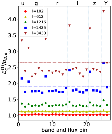
The relation is less accurate in photometric redshift space. Due to significant photo-z uncertainties, the true redshift distribution of photo-z galaxy samples is inevitably wide. This mixes different scale and galaxy intrinsic properties. We test the validity of Eq. 5 in the 2D angular clustering against CosmoDC2. CosmoDC2 is the galaxy mock generated for LSST (Korytov et al., 2019). It provides a lightcone of , with billion galaxies to . The magnitudes in photometry bands are also provided. Such multi-band photometry information is crucial for our method. Since CosmoDC2 does not provide the underlying dark matter density light cones, we map CosmoDC2 galaxies to a CosmicGrowth simulation (Jing, 2019), based on halo abundance matching. We then randomly add photo-z errors of to mock galaxies, and generate 20 lightcones, each of size . Details of the simulations and the mocks are described in §A.
Table 1 shows the definition of galaxy sub-samples in photometry bands and flux bins in total ( flux bins in bands respectively). Unless otherwise specified, these will be the default galaxy samples for tests in this paper. We have investigated multipole photometric redshift bins for lensing reconstruction. Since the method is found to be applicable in all cases, we only show the default photometric redshift range , for brevity. The number density of galaxies, ranging from arcmin-2 to arcmin-2, varies significantly with the photometry band (and the associated magnitude cut).
Fig. 1 shows for the above galaxy sub-samples. The proportionality relation (Eq. 5) is nearly exact at and remains reasonably valid until The accuracy of the proportionality relation also depends on the flux bins. The bins that deviates the most from the proportionality relation are the brightest galaxies in the given photometry bands (e.g. the uppermost 6 data points of Fig. 1). Therefore the behavior may be related to the nonlinear bias of these brightest galaxies. One issue is whether or not to use these bins in the cosmic magnification reconstruction. Disregarding them indeed reduces the systematic bias due to better proportionality relation. But on the other hand, it enhances the statistical errors. The reason is that the magnification coefficient in these bins are significantly different to other bins. Without these bins, the weighting scheme designed later is less efficient and the reconstruction uncertainty is enhanced. The combined consequence is that disregarding them does not improve the overall reconstruction performance. Therefore for the rest of the paper, we will include these bins in the analysis. Nevertheless, this issue deserves further investigation, in mock data and in real data analysis.
We can then determine by the following three conditions,
| (6) |
| (7) |
| (8) |
The first condition (Eq. 6) is to make the estimation free of multiplicative bias, given the magnification response parameter . The second (Eq. 7) is to eliminate the deterministic galaxy bias. The third is to minimize the shot noise. The three conditions fix
| (9) |
Here , and . is the shot noise matrix. The method is identical to that in Hou et al. (2021) proposed by some of the authors, but with two important improvements by replacing the approximate condition (Hou et al., 2021) with Eq. 7, and by including multiple photometry band information.
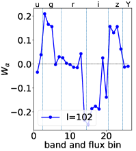
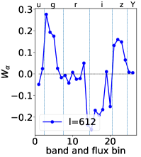

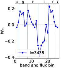
Fig. 2 shows the weight at various multipole . The dependence on is visible. This is induced by the condition Eq. 7 through . also changes sign. This is also the consequence of the condition Eq. 7. Interestingly, the mean is a factor of than the typical value of (Fig. 9). So the approximation adopted by Hou et al. (2021) is roughly satisfied. When we are not able to infer robustly from observations (e.g. with the presence of uncorrected selection effects affecting the clustering measurement), the method of Hou et al. (2021) will be a viable alternative.
3 The performance
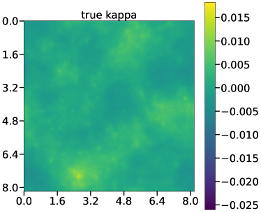
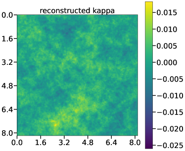
One of the reconstructed maps is shown in Fig. 10. The maps are noisy due to overwhelming shot noise. Therefore we have to quantify the reconstruction performance statistically. Other than shot noise fluctuation, the reconstructed map is
| (10) |
The above relation comes from Eq. 4, together with Eq. 1, 2 & 3. The error term is caused by stochastic galaxy bias. It can be down-weighted, but not eliminated by our method. This term is uncorrelated with the matter overdensity in the two-point correlation. So it does not induce systematic errors in cross-correlation with external weak lensing data sets, such as cosmic shear and CMB lensing. It contaminates the auto-correlation measurement. But it is sub-dominant comparing to the shot noise fluctuation from discrete galaxy distribution.
3.1 Residual deterministic bias
The term is analogous to the galaxy intrinsic alignment in the cosmic shear measurement. It contaminates both the auto and cross power spectrum measurements.
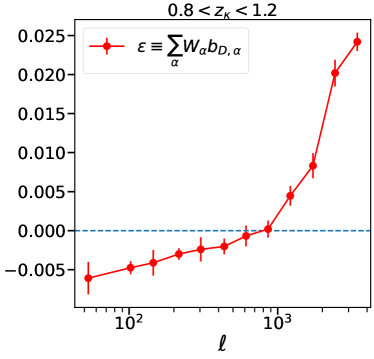
Since the proportionality relation (Eq. 5) is not completely exact and since in reality suffers from shot noise, cosmic variance, magnification bias and other observational effects, the condition Eq. 7 does not guarantee removal of deterministic galaxy clustering. The residual error in the reconstruction is . Here
| (11) |
Fig. 3 shows that at , but increases to - at . The negative at is surprising, since naively we may expect that at such large scale the galaxy stochasticity vanishes and . This may be caused by statistical fluctuations in due to limited number of multipole modes. These statistical fluctuations in , after the nonlinear matrix operation process, become systematic error in . Furthermore, even if is free of errors, other nonlinear matrix operations in finding the weight through Eq. 9 will render other statistical errors into systematic errors. These systematic errors then lead to , which can be significant at large scales due to smaller modes and larger statistical fluctuations. This behavior (chance correlation) has been observed in CMB foreground removal with the internal linear combination (ILC) method (e.g. Saha et al. (2008); Vio & Andreani (2008)). ILC is similar to our weighting scheme. It is also a linear estimator, with Eq. 6 replaced by the condition of unbiased CMB amplitude and Eq. 8 replaced by minimizing the variance of weighted maps. Given the resemblance in the math structure, we suspect that the at large scale found here has similar origins as that in ILC. Since it is not the dominant source of systematic errors, we postpone its further investigation. On the other hand, at is expected from Fig. 1, since the scaling relation is no longer as accurate as the case of . increases quickly with increasing and reaches at . This will be the dominant systematic error in the reconstruction.
3.2 The auto-correlation error budget
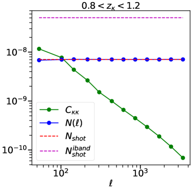
The map quality can be quantified by contaminations in the auto power spectrum,
| (12) |
The noise power spectrum includes the auto power spectra of shot noise, and . It also includes the - cross term. To calculate , we calculate directly from the reconstructed maps and from the maps of the true signal. We then subtract from to obtain . The resulting is shown in Fig. 4. We also compare it to the weighted shot noise , which is calculated using Eq. 8 given the weights. Fig. 4 shows that the error budget is dominated by , namely . The reconstructed map is signal dominated at , and is noise dominated at . The map is not as clean as the shear maps or CMB lensing maps, which will reach the cosmic variance limit at (e.g. Abazajian et al. (2016)). The comparison here assumes the same number of galaxies for cosmic magnification and cosmic shear. But in principle there are more galaxies to use for cosmic magnification than for cosmic shear, since galaxy detection is easier than galaxy shape measurement. Therefore there are still rooms for improving the cosmic magnification reconstruction, by including more galaxies at faint end.
One valuable lesson is to use as many photometry bands as possible. The noise power spectrum when using photometry bands is a factor of smaller that of using only the band (Fig. 4). The relative ranking of galaxy brightness varies in different photometry bands. It has two-fold impacts on improving the reconstruction. First, galaxies have different in different photometry bands. This source of cosmic magnification information significantly improves the reconstruction. Second, shot noise in flux bins of different photometry bands is different. So combining all the flux bins reduce shot noise.
3.3 S/N estimation of cross-correlation with external fields
Although the reconstructed map will have large noise and the resulting auto power spectrum measurement S/N is hard to compete with cosmic shear or CMB lensing, the cross-correlation with external lensing fields is significantly cleaner. The reason is that none of and shot noise biases the two-point statistics. Only the residual deterministic component of galaxy clustering induces bias in the cross-correlation measurement. The resulting two-point correlation function is
| (13) |
Here stands for the convergence field from external data such as cosmic shear and CMB lensing. This type of cross-correlation has been proposed and measured in HSC by Liu et al. (2021).
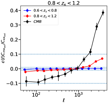
Since the matter distribution is only correlated with weak lensing at higher source redshift, causes non-negligible contamination to only when the source redshifts of external lensing fields are higher than that of cosmic magnification, and only when . Fig. 5 shows the resulting errors in cross-correlation with cosmic shear and CMB lensing. For cosmic magnification reconstructed at , its cross-correlation with cosmic shear at has negligible systematic error. Due to the redshift range and the extra broadening caused by photo-z errors, the systematic error becomes significant at when . The error increases with increasing . So the situation is most severe for CMB lensing.
The S/N of cross-correlation measurement, if only statistical error is considered, can be estimated by
| (14) |
Here is the multipole bin size and is the sky coverage. We adopt (LSST Science Collaboration et al., 2009). is the noise power spectrum of the external lensing field. This estimation does not consider super sample covariance (Takada & Hu, 2013) or non-Gaussian covariance (Takada & Jain, 2009), which will decrease the S/N. Since the decrement is moderate (e.g. Yao et al. (2023)), we will adopt this simplification of Eq. 14 to demonstrate the potential of cosmic magnification reconstruction. The estimated S/N is shown in Fig. 6.
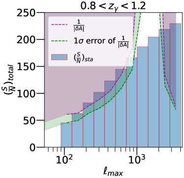
However, the above raw estimation of S/N is not realistic, due to the systematic error, which puts an upper limit on the realistic S/N. Since it varies with scale, we quantify its impact on the overall amplitude of the measured cross power spectrum. Namely we try to fit the data with . means vanishing weighted systematic error. The bias in is then
| (15) |
Therefore a realistic estimation of S/N is
| (16) |
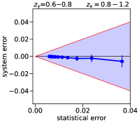
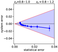
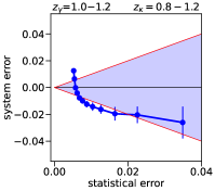
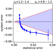
Fig. 6 shows the S/N expected by cross-correlating with cosmic shear at , for a LSST-like survey. Cross-correlation measurement with at can be achieved. Fig. 12 shows the statistical and systematic errors for multipole bins.
Systematic errors, in particular at , can be further mitigated. Fig. 12 shows more detailed comparison between the statistical and systematic errors, for multipole bins. It shows that two behave differently in the space. For example, the raw measurement of can be fitted by of multiple bins. Since does not vary with , we can break the degeneracy between and with multiple (cosmic shear redshift ranges). We will leave such investigations until further study.
4 Conclusion
We propose a minimum variance linear estimator to reconstruct the weak lensing convergence map, by weighing overdensity maps of galaxies in different magnitude bins and different photometry bands. This estimator efficiently suppresses the major contamination of galaxy intrinsic clustering. In particular, it is able to suppress the deterministic part of the galaxy intrinsic clustering by a factor of (Fig. 3). Therefore the reconstructed map is nearly free of galaxy clustering contamination in its cross correlation with cosmic shear at . Based on the CosmoDC2 galaxy mock and the CosmicGrowth simulation, we validate this method. We also forecast that a LSST-like survey can achieve through cross-correlations between the reconstructed convergence map and cosmic shear, with systematic errors under control.
There are important issues for further investigation. (1) One is to further suppress the residual galaxy clustering in the convergence-shear cross-correlation measurement. Such systematic error becomes dominant at and when the shear source redshift is higher than the convergence source redshift (Fig. 12). We believe that it can be further reduced, since we know that it is proportional to the matter-cosmic shear cross-correlation . The only unknown parameter is its amplitude . varies with (Fig. 3), but not . Therefore by joint analysis of cross-correlations of multiple , we can simultaneously constrain cosmological parameters and . (2) Although the reconstructed lensing convergence map can deliver high S/N cross-correlation measurement with cosmic shear and CMB lensing, auto power spectrum measurement in the current investigation is not competitive with respect to cosmic shear and CMB lensing (Fig. 4). However, there are still possibilities to improve. The lesson learn from the current investigation is to weigh over as many galaxy overdensity maps as possible. In this work we use maps defined by magnitude cut in the photometry bands. Zhou et al. (2023) found that galaxy sub-samples defined in the color-space are also useful in understanding and controlling galaxy bias (clustering). Since gravitational lensing does not change color, the cosmic magnification (magnification bias) in the color bins has when we ignore any other selection effects. This means that including galaxy sub-samples in the color space and the associated overdensity map, the lensing reconstruction can be further improved, in both S/N and systematic errors.
Acknowledgement
This work is supported by National Science Foundation of China (11621303, 12273020, 11890690), the National Key R&D Program of China (2020YFC2201602), the China Manned Space Project (#CMS-CSST-2021-A02 & CMS-CSST-2021-A03), and the Fundamental Research Funds for the Central Universities. YY thanks the sponsorship from Yangyang Development Fund.
Data Availability
The data underlying this article will be shared on reasonable request to the corresponding author.
References
- Abazajian et al. (2016) Abazajian K. N., et al., 2016, arXiv e-prints, p. arXiv:1610.02743
- Albrecht et al. (2006) Albrecht A., et al., 2006, ArXiv Astrophysics e-prints,
- Amendola et al. (2016) Amendola L., et al., 2016, preprint, (arXiv:1606.00180)
- Amon et al. (2022) Amon A., et al., 2022, Phys. Rev. D, 105, 023514
- Baldauf et al. (2010) Baldauf T., Smith R. E., Seljak U., Mandelbaum R., 2010, Phys. Rev. D, 81, 063531
- Bonavera et al. (2021) Bonavera L., Cueli M. M., González-Nuevo J., Ronconi T., Migliaccio M., Lapi A., Casas J. M., Crespo D., 2021, A&A, 656, A99
- Bonoli & Pen (2009) Bonoli S., Pen U. L., 2009, MNRAS, 396, 1610
- Elvin-Poole et al. (2022) Elvin-Poole J., et al., 2022, arXiv e-prints, p. arXiv:2209.09782
- Euclid Collaboration et al. (2022) Euclid Collaboration et al., 2022, A&A, 662, A93
- Garcia-Fernandez et al. (2018) Garcia-Fernandez M., et al., 2018, MNRAS, 476, 1071
- Gong et al. (2019) Gong Y., et al., 2019, ApJ, 883, 203
- González-Nuevo et al. (2014) González-Nuevo J., et al., 2014, MNRAS, 442, 2680
- González-Nuevo et al. (2021) González-Nuevo J., Cueli M. M., Bonavera L., Lapi A., Migliaccio M., Argüeso F., Toffolatti L., 2021, A&A, 646, A152
- Hamaus et al. (2010) Hamaus N., Seljak U., Desjacques V., Smith R. E., Baldauf T., 2010, Phys. Rev. D, 82, 043515
- Heitmann et al. (2019) Heitmann K., et al., 2019, The Astrophysical Journal Supplement Series, 245, 16
- Hildebrandt et al. (2009) Hildebrandt H., van Waerbeke L., Erben T., 2009, A&A, 507, 683
- Hildebrandt et al. (2013) Hildebrandt H., et al., 2013, MNRAS, 429, 3230
- Hoekstra & Jain (2008) Hoekstra H., Jain B., 2008, Annual Review of Nuclear and Particle Science, 58, 99
- Hou et al. (2021) Hou S.-T., Yu Y., Zhang P.-J., 2021, Research in Astronomy and Astrophysics, 21, 247
- Jain (2002) Jain B., 2002, ApJ, 580, L3
- Jalilvand et al. (2020) Jalilvand M., Majerotto E., Bonvin C., Lacasa F., Kunz M., Naidoo W., Moodley K., 2020, Phys. Rev. Lett., 124, 031101
- Jing (2019) Jing Y., 2019, Science China Physics, Mechanics, and Astronomy, 62, 19511
- Korytov et al. (2019) Korytov D., et al., 2019, ApJS, 245, 26
- LSST Dark Energy Science Collaboration (2012) LSST Dark Energy Science Collaboration 2012, preprint, (arXiv:1211.0310)
- LSST Science Collaboration et al. (2009) LSST Science Collaboration et al., 2009, preprint, (arXiv:0912.0201)
- Lewis et al. (1999) Lewis A., Challinor A., Lasenby A., 1999, The Astrophysical Journal, 538, 473
- Li et al. (2023) Li X., et al., 2023, arXiv e-prints, p. arXiv:2304.00702
- Liu et al. (2021) Liu X., Liu D., Gao Z., Wei C., Li G., Fu L., Futamase T., Fan Z., 2021, Phys. Rev. D, 103, 123504
- Ménard et al. (2010) Ménard B., Scranton R., Fukugita M., Richards G., 2010, MNRAS, 405, 1025
- Planck Collaboration et al. (2020) Planck Collaboration et al., 2020, A&A, 641, A8
- Qu et al. (2023) Qu F. J., et al., 2023, arXiv e-prints, p. arXiv:2304.05202
- Refregier (2003) Refregier A., 2003, ARA&A, 41, 645
- Saha et al. (2008) Saha R., Prunet S., Jain P., Souradeep T., 2008, Phys. Rev. D, 78, 023003
- Schmidt et al. (2012) Schmidt F., Leauthaud A., Massey R., Rhodes J., George M. R., Koekemoer A. M., Finoguenov A., Tanaka M., 2012, ApJ, 744, L22
- Scranton et al. (2005) Scranton R., et al., 2005, ApJ, 633, 589
- Takada & Hu (2013) Takada M., Hu W., 2013, Phys. Rev. D, 87, 123504
- Takada & Jain (2009) Takada M., Jain B., 2009, MNRAS, 395, 2065
- Tegmark & Bromley (1999) Tegmark M., Bromley B. C., 1999, ApJ, 518, L69
- Vallinotto et al. (2011) Vallinotto A., Dodelson S., Zhang P., 2011, Phys. Rev. D, 84, 103004
- Vio & Andreani (2008) Vio R., Andreani P., 2008, A&A, 487, 775
- Wang et al. (2011) Wang L., et al., 2011, MNRAS, 414, 596
- Weinberg et al. (2013) Weinberg D. H., Mortonson M. J., Eisenstein D. J., Hirata C., Riess A. G., Rozo E., 2013, Phys. Rep., 530, 87
- Yang & Zhang (2011) Yang X., Zhang P., 2011, MNRAS, 415, 3485
- Yang et al. (2015) Yang X., Zhang P., Zhang J., Yu Y., 2015, MNRAS, 447, 345
- Yang et al. (2017) Yang X., Zhang J., Yu Y., Zhang P., 2017, ApJ, 845, 174
- Yao et al. (2023) Yao J., et al., 2023, arXiv e-prints, p. arXiv:2304.04489
- Zhan & Tyson (2018) Zhan H., Tyson J. A., 2018, Reports on Progress in Physics, 81, 066901
- Zhang & Pen (2005) Zhang P., Pen U.-L., 2005, Phys. Rev. Lett., 95, 241302
- Zhang et al. (2018) Zhang P., Yang X., Zhang J., Yu Y., 2018, ApJ, 864, 10
- Zhang et al. (2019) Zhang P., Zhang J., Zhang L., 2019, MNRAS, 484, 1616
- Zhou et al. (2023) Zhou S., Zhang P., Chen Z., 2023, arXiv e-prints, p. arXiv:2304.11540
- von Wietersheim-Kramsta et al. (2021) von Wietersheim-Kramsta M., et al., 2021, MNRAS, 504, 1452
Appendix A The mocks for the tests
We use CosmoDC2 to test our method. CosmoDC2 is the galaxy mock generated for LSST (Korytov et al., 2019). It provides a lightcone of , with billion galaxies to . The magnitudes in photometry bands are also provided. Such multi-band photometry information is crucial for our method. CosmoDC2 also provides the host halo information of these galaxies. A problem is that, CosmoDC2 itself does not provide the associated 3D matter density field, which is based on the Outer Rim simulation (Heitmann et al., 2019). Since we need the underlying density field for our analysis, we combine CosmoDC2 with our CosmicGrowth simulations (Jing, 2019). The CosmicGrowth simulation we use has a flat CDM cosmology with , , , & . The simulation has box size of , and particle number of . We use the galaxy-host halo information of CosmoDC2 to assign galaxies to the CosmicGrowth simulation halos. The bottom line is to have the same amount of galaxies about the same magnitude in both simulations. Since CosmoDC2 only contains halos hosting galaxies, we compare the CosmoDC2 halo mass function with the halo mass function predicted by the CosmoDC2 cosmology to figure out the fraction of halos of given mass hosting CosmoDC2 galaxies. Since the cosmological parameters in the two simulations are not identical, the two have different halo mass functions. We first do an abundance matching between the halo mass function predicted by the CosmoDC2 cosmology and that by the CosmicGrowth cosmology. This tells us the mass of halos in CosmicGrowth corresonding to that in CosmoDC2. Then we can match each halo in CosmoDC2 with the corresponding halo (or one of the corresponding halos) in CosmicGrowth, we transport all galaxies in the CosmoDC2 halo to the CosmicGrowth halo, including the distinction of central and satellite galaxies and their relative positions. We caution that this procedure of transporting CosmoDC2 galaxies to other simulations is only approximate, since properties other than the halo mass (e.g. halo ellipticity, environment and history) also affect galaxy formation. In the future we should use more realistic galaxy mocks to test our method.
We generate 20 light-cones of 3D galaxy positions and photometry information to , each of size . We then add random redshift scatter of r.m.s. to mock galaxies. Magnitude cuts are applied to define galaxy sub-samples for the galaxies with , as shown in Table 1. These galaxy sub-samples are used to generate maps of (unlensed) galaxy overdensity on uniform grids. We also generate corresponding light cones of matter distribution and weak lensing map at various source redshifts (including for CMB lensing). We use Eq. 1 to combine the galaxy ovendensity maps and the lensing convergence maps into the lensed galaxy overdensity maps, with measured from the luminosity function of mock galaxies.
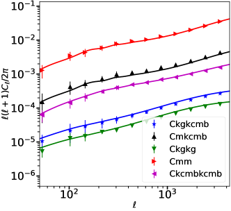
We check the validity of the generated maps by measuring the corresponding power spectra. Fig. 7 shows the measurements of for the source redshift . It agrees with the theoretical prediction via CAMB (Lewis et al., 1999). It also shows . Besides the correct auto-correlation statistics, the maps also have correct cross-correlations, such as the matter(galaxy)-CMB lensing cross-correlation and galaxy lensing-CMB lensing cross-correlation .
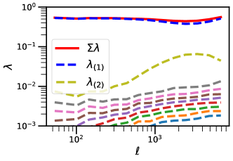
We then measure the galaxy correlation matrix (). Here is for our fiducial galaxy sample. Notice that also include contributions from cosmic magnification. The eigenvalues, as a function of , are shown in Fig. 8. The matrix is dominated by the largest eigenmode, while the second largest eigenmode is also statistically significant. These behaviors are consistent with previous findings (Bonoli & Pen, 2009; Hamaus et al., 2010).
We test the proposed proportionality relation between the largest eigenvector and the galaxy deterministic bias (Eq. 5). As a reminder, denotes the -th galaxy sub-sample. Fig. 1 shows that this relation holds accurately at and reasonably well at . This is consistent with our finding in 3D galaxy clustering (Zhou et al., 2023). Results present here show that the proportionality relation is robust against mixing of different mode due to the projection effect in angular clustering. Therefore we are able to use Eq. 5 to construct the optimal weight of reconstructing the lensing convergence maps. Notice that for the estimator, the proportionality coefficient does not matter.
Fig. 9 shows an interesting result that . More exactly, is a factor of smaller than typical (Fig. 2). This means that in reality the condition adopted by the previous proposal (Hou et al., 2021) is reasonably satisfied. For this reason, we may adopt the condition as a first attempt to analyze real data.111Jian Qin, et al, in preparation. This version of lensing convergence reconstruction, although sub-optimal in suppressing , is applicable to galaxy catalogs without accurate galaxy clustering measurement.

Appendix B Statistical and systematic errors
B.1 The reconstructed maps
Fig. 10 shows one of the reconstructed maps. The reconstruction is noisy, due to shot noise overwhelming at most scales. For this reason, we only present the Wiener filtered maps with , in which both the lensing power spectrum and the noise (mostly shot noise) power spectrum are defined in the main text. The process of Wiener filter reveals similarity of and at degree scale and above. This is consistent with Fig. 4.
B.2 The raw SNR
The raw SNR, namely the signal-to-noise ratio only considering statistical errors, is shown in Fig. 11. The bottom left panel shows the SNR of each bin, for fixed convergence map constructed using galaxies at . The cross correlation is done with cosmic shear at various source redshifts . The peak contribution occurs at , where statistical errors from cosmic variance and shot noise roughly balance. The bottom right panel shows the total SNR up to or , for various . The maximum SNR is achieved when , where the cross-correlation coefficient of the two lensing fields (cosmic convergence and shear) is the largest. For , the total SNR using all modes is about .
B.3 Systematic error versus statistical error
The raw SNR is the optimistic case where systematic errors are ignored. As Fig. 3 & 5 show, the systematic error due to imperfect correction of deterministic galaxy bias presents at all . Its impact on the cross-correlation measurement is negligible when the cosmic shear redshift . The reason is that this contamination is induced by the residual deterministic galaxy bias and is therefore uncorrelated with cosmic shear at lower redshifts. But when , this contamination will become more and more significant (Fig. 5).
Since both the amplitude and the sign of this systematic error varies with the angular scale, we adopt a commonly used weighting to weigh its overall impact at and compress the overall systematic error into a single parameter (Eq. 15). Fig. 12 shows the plot of the systematic error () versus the statistical error (). For brevity, we only show the result for the lensing convergence map reconstructed using galaxies in the photometric redshift range . The cosmic shear source redshifts are from to . As expected, since the residual galaxy clustering only correlates with cosmic shear at higher redshifts, its contamination to the cross-correlation measurement with lower redshift (e.g. ) cosmic shear is negligible.222Notice that in such case the contamination is non-zero due to photo-z errors. For this reason, we do not show the results at even lower cosmic shear source redshift. When , the systematic error begins to dominate over the statistical error when the raw S/N reaches and prohibits more accurate measurement. The situation becomes worse for and even higher redshifts.
Mitigating these significant systematic errors will be a remaining major issue. As we have discussed in §4, there are promising approaches to correct such errors efficiently, either with a joint analysis of multipole cross-correlation measurements or with reconstruction of galaxy sub-samples in color space. These will be major tasks of future investigation.
