An information projection approach to robust propensity score estimation under missing at random

Abstract

Missing data is frequently encountered in many areas of statistics. Propensity score weighting is a popular method for handling missing data. The propensity score method employs a response propensity model, but correct specification of the statistical model can be challenging in the presence of missing data. Doubly robust estimation is attractive, as the consistency of the estimator is guaranteed when either the outcome regression model or the propensity score model is correctly specified. In this paper, we first employ information projection to develop an efficient and doubly robust estimator under indirect model calibration constraints. The resulting propensity score estimator can be equivalently expressed as a doubly robust regression imputation estimator by imposing the internal bias calibration condition in estimating the regression parameters. In addition, we generalize the information projection to allow for outlier-robust estimation. Some asymptotic properties are presented. The simulation study confirms that the proposed method allows robust inference against not only the violation of various model assumptions, but also outliers. A real-life application is presented using data from the Conservation Effects Assessment Project.

1 Introduction

Missing data is a fundamental problem in statistics. Ignoring missing data can lead to biased estimates of parameters, loss of information, decreased statistical power, increased standard errors, and weak generalizability of findings (Dong and Peng,, 2013). Propensity score weighting is a popular method to handle missing data. It often employs a response propensity model, but correct specification of the statistical model can be challenging in the presence of missing data. How to make the propensity score weighting method less dependent on the response propensity model is an important practical problem.

There are two main approaches to implement robust propensity score estimation. One approach is to use a flexible model, nonparametric or semiparametric, to develop a robust propensity score estimation method. The nonparametric kernel method Hahn, (1998), the sieve logistic regression method (Hirano et al.,, 2003), the general calibration method of Chan et al., (2016) using increasing dimension of the basis functions, the generalized covariate balancing estimator using tailor loss functions (Zhao,, 2019) and the random forest approach of Dagdoug et al., (2023) are examples of the robust propensity score estimation method using flexible models. The other approach is to use the outcome regression model explicitly to obtain a doubly robust estimation. Doubly robust estimation has been extensively investigated in the literature. For examples, see Bang and Robins, (2005), Cao et al., (2009), Yang et al., (2020).

In this paper, we consider the second approach and develop a unified framework for doubly robust propensity score (PS) estimation under the setup of missing at random (Rubin,, 1976). Specifically, we apply the information projection (Csiszár and Shield,, 2004) to the PS weighting problem under the covariate-balancing constraints. The initial weights of the PS are obtained from the working PS model, but the balancing constraints in the information projection are obtained from the working outcome regression model. Imposing covariate-balancing constraints can be understood as indirect model calibration. Indirect model calibration is the key condition to achieve double robustness in the PS weighting estimator. Information projection is used to obtain the augmented PS model.

The resulting PS weighting estimator can also be expressed as a regression imputation estimator using the balancing functions as covariates in the outcome regression model. This algebraical equivalence, called self-efficiency, is useful in developing outlier robust PS estimation. Outliers in the outcome variable often significantly reduce the efficiency of the resulting estimator. How to reduce the effect of outliers into estimation is a very important problem in statistics. While outlier-robust procedures are well studied in the literature on regression or classification (Stefanski et al.,, 1986; Wu and Liu,, 2007; Zhang et al.,, 2010), it is not fully developed in the context of missing data. To our knowledge, constructing an outlier robust propensity score estimator has not been investigated in the literature. To solve this challenging problem, we first develop an outlier-robust regression imputation and then express it as a PS weighting estimator by incorporating a condition for self-efficiency.

The information projection approach to developing the augmented PS model and obtaining the doubly robust estimation is based on the Kullback-Leibler divergence. The Kullback-Leibler-divergence-based projection method is useful in incorporating the moment-type constraints. The $\gamma$-power divergence, originally proposed by Basu et al., (1998) and further developed by Eguchi, (2021), is a generalization of the Kullback-Leibler divergence to expand the class of statistical models by introducing an additional scale parameter $\gamma$. Furthermore, it is well known that the statistical model derived from $\gamma$-power divergence produces robust inferences against outliers. We adopt the $\gamma$-power divergence to develop an outlier-robust regression imputation estimator. By self-efficiency, the regression estimator can be expressed as a PS weighting estimator. The resulting estimator is also robust against misspecification of the response probability model.

The structure of the paper is as follows. In Section 2, the basic setup and the research problem are introduced. In Section 3, we develop a balancing constraint to adjust propensity weights and construct an augmented propensity model using information projection. In Section 4, we present the use of the $\gamma$-power divergence to enlarge the class of propensity score models and develop outlier-robust doubly robust estimators. Extension to causal inference is discussed in Section 5. The simulation study in Section 6 shows the usefulness of the proposed method. A real-life application using data from the Conservation Effects Assessment Project is presented in Section 7. Some concluding remarks are made in Section 8. All required evidences are presented in the Appendix.

2 Basic Setup

Suppose that there are $n$ independently and identically distributed realizations of $(\boldsymbol{X},Y,\delta)$, denoted by $\{(\boldsymbol{x}_{i},y_{i},\delta_{i}):i=1,\ldots,n\}$, where $\boldsymbol{x}_{i}$ is a vector of observed covariates and $\delta_{i}$ is the missingness indicator associated with unit $i$. In particular, $\delta_{i}=1$ if $y_{i}$ is observed and $\delta_{i}=0$ otherwise. Thus, instead of observing $(\boldsymbol{x}_{i},y_{i},\delta_{i})$, we only observe $(\boldsymbol{x}_{i},\delta_{i},\delta_{i}y_{i})$ for $i=1,\ldots,n$. We are interested in estimating $\theta=E(Y)$ from the observed sample.

Suppose that we have a working outcome regression model given by

$$m_{0}\left(\boldsymbol{x};\boldsymbol{\beta}\right)\in\mbox{span}\{{b}_{0}(\boldsymbol{x})\equiv 1,{b}_{1}(\boldsymbol{x}),\ldots,{b}_{L}(\boldsymbol{x})\}$$ (1)

for some given basis functions ${b}_{1}(\boldsymbol{x}),\ldots,{b}_{L}(\boldsymbol{x})$. The model (1) can be expressed equivalently as

$$y_{i}=m(\boldsymbol{x}_{i};\boldsymbol{\beta})+\varepsilon_{i},~{}m(\boldsymbol{x}_{i};\boldsymbol{\beta})=\beta_{0}+\beta_{1}{b}_{1}(\boldsymbol{x}_{i})+\ldots+\beta_{L}{b}_{L}(\boldsymbol{x}_{i})$$

for $\beta=(\beta_{0},\beta_{1},\ldots,\beta_{L})^{\operatorname{T}}$, where $\varepsilon_{i}$ is an error term that is independent of $\boldsymbol{x}_{i}$ and satisfies $E(\varepsilon_{i})=0$. Furthermore, the assumption of missing at random (Rubin,, 1976) implies that $\varepsilon_{i}$ and $\delta_{i}$ are conditionally independent given $\boldsymbol{x}_{i}$.

We are interested in using the following propensity score weighting (PSW) estimator

$$\hat{\theta}_{\rm PSW}=\frac{1}{n}\sum_{i=1}^{n}\delta_{i}\omega_{i}y_{i}.$$ (2)

The following lemma provides a sufficient condition for the unbiasedness of the propensity score weighting estimators under the model (1).

Lemma 2.1.

Assume that the response mechanism is missing at random. If the weights $\omega_{i}$’s satisfy

$$\sum_{i=1}^{n}\delta_{i}\omega_{i}\left[{b}_{0}(\boldsymbol{x}_{i}),{b}_{1}(\boldsymbol{x}_{i}),\ldots,{b}_{L}(\boldsymbol{x}_{i})\right]=\sum_{i=1}^{n}\left[{b}_{0}(\boldsymbol{x}_{i}),{b}_{1}(\boldsymbol{x}_{i}),\ldots,{b}_{L}(\boldsymbol{x}_{i})\right],$$ (3)

then $\hat{\theta}_{\rm PSW}$ in (2) is unbiased for $\theta$ under the outcome regression model in (1).

By Lemma 3, condition (3) is the key condition that incorporates the outcome regression model into the PSW estimator. Condition (3) is often called the covariate balancing condition (Imai and Ratkovic,, 2014) in the missing data literature. It is closely related to the calibration estimation in survey sampling (Deville and Särndal,, 1992). Because the balancing functions in (3) are equal to the basis functions of the outcome regression model in (1), we can achieve

$$\sum_{i=1}^{n}\delta_{i}\omega_{i}E(Y_{i}\mid\boldsymbol{x}_{i})=\sum_{i=1}^{n}E(Y_{i}\mid\boldsymbol{x}_{i}),$$ (4)

which is often referred to as the model calibration (Wu and Sitter,, 2001). To distinguish from the direct model calibration of Wu and Sitter, (2001), we may call (3) the indirect model calibration.

The indirect model calibration condition also implies the following algebraic equivalence.

Lemma 2.2.

If the weights $\omega_{i}$ satisfy (3), then we have

$$\sum_{i=1}^{n}\delta_{i}\omega_{i}y_{i}=\sum_{i=1}^{n}\{\delta_{i}y_{i}+(1-\delta_{i})\boldsymbol{{b}}_{i}^{\operatorname{T}}\hat{\boldsymbol{\beta}}\},$$ (5)

where $\hat{\boldsymbol{\beta}}$ satisfies

$$\sum_{i=1}^{n}\delta_{i}\left(\omega_{i}-1\right)\left(y_{i}-\boldsymbol{{b}}_{i}^{\operatorname{T}}\hat{\boldsymbol{\beta}}\right)=0.$$ (6)

and $\boldsymbol{{b}}_{i}=(1,{b}_{1}(\boldsymbol{x}_{i}),\ldots,{b}_{L}(\boldsymbol{x}_{i}))^{\operatorname{T}}$.

Lemma 6 means that, under (6), the PSW estimator that satisfies the covariate-balancing condition is algebraically equivalent to a regression imputation estimator using the balancing functions as covariates in the outcome regression model. In other words, regression imputation under the outcome regression model in (1) can be viewed as a propensity score weighting estimator where the propensity score weights $\omega_{i}$ and the estimated regression coefficients $\hat{\boldsymbol{\beta}}$ are related by equation (6). Equation (5) means that the final propensity score weights ${\omega}_{i}$ do not directly use the outcome regression model (1) for imputation, but implement regression imputation indirectly. Condition (5) is referred to as the self-efficiency condition.

We now wish to achieve double robustness by including the propensity score model. In the working propensity score model, the propensity score weights are computed as $\omega_{i}=\{\pi(\boldsymbol{x}_{i};\hat{\boldsymbol{\phi}})\}^{-1}:=\hat{d}_{i}$, where $\hat{\boldsymbol{\phi}}$ is the maximum likelihood estimation of $\boldsymbol{\phi}$. However, the propensity score $\hat{d}_{i}$ does not necessarily satisfy the balancing condition in (3). Therefore, to reduce the bias due to model misspecification in the propensity score model, it makes sense to impose the balancing condition in the final weighting. To achieve this goal, Hainmueller, (2012) proposed the so-called entropy balancing method that minimizes

$$Q(\boldsymbol{\omega})=\sum_{i=1}^{n}\delta_{i}\omega_{i}\log(\omega_{i}/\hat{d}_{i}),$$ (7)

subject to the balancing constraint in (3). Using the Lagrange multiplier method, the solution takes the form of

$$\hat{\omega}_{i}=\frac{\hat{d}_{i}\exp\left(\boldsymbol{{b}}_{i}^{\operatorname{T}}\hat{\boldsymbol{\lambda}}\right)}{\sum_{k=1}^{n}\left\{\delta_{k}\hat{d}_{k}\exp\left(\boldsymbol{{b}}_{k}^{\operatorname{T}}\hat{\boldsymbol{\lambda}}\right)\right\}},$$

where $\hat{\boldsymbol{\lambda}}$ is chosen to satisfy the covariate balancing condition. Chan et al., (2016) generalized this idea further to develop a general calibration weighting method that satisfies the covariance balancing property with increasing dimensions of basis functions $\boldsymbol{{b}}(\boldsymbol{x})$.

3 Proposed method

3.1 Information projection

We now develop an alternative approach to modifying the initial propensity score weights to satisfy the covariate balancing condition in (3). Instead of using a distance measure for propensity weights, as in (7), we use the Kullback-Leibler divergence measure to develop the information projection under some moment constraint. Because the Kullback-Leibler divergence is defined in terms of density functions, we need to formulate the weighting problem as an optimization problem for density functions.

To apply the information projection, using the Bayes theorem, we obtain

$$\frac{{P}(\delta=0\mid\boldsymbol{x})}{{P}(\delta=1\mid\boldsymbol{x})}=\frac{1-p}{p}\times\frac{f_{0}(\boldsymbol{x})}{f_{1}(\boldsymbol{x})},$$

where $p={P}(\delta=1)$ and $f_{k}(\boldsymbol{x})=f(\boldsymbol{x}\mid\delta=k)$ for $k=0,1$. Thus, the propensity score (PS) weight can be written as

$$\omega(\boldsymbol{x})\equiv\frac{1}{{P}(\delta=1\mid\boldsymbol{x})}=1+c\times\frac{f_{0}(\boldsymbol{x})}{f_{1}(\boldsymbol{x})}.$$ (8)

where $c=1/p-1$. Furthermore, assume that the basis function ${\boldsymbol{{b}}}(\boldsymbol{x})$ in the outcome regression model in (1) is integrable in the sense that

$$pE_{1}\{\boldsymbol{{b}}(\boldsymbol{X})\}+(1-p)E_{0}\{\boldsymbol{{b}}(\boldsymbol{X})\}=E\{\boldsymbol{{b}}(\boldsymbol{X})\},$$ (9)

where $E_{k}\{\boldsymbol{{b}}(\boldsymbol{X})\}=\int\boldsymbol{{b}}(\boldsymbol{x})f_{k}(\boldsymbol{x})d\mu(\boldsymbol{x})$ for $k=0,1$. If $E\{\boldsymbol{{b}}(\boldsymbol{X})\}$ is known, we can impose a constraint on $f_{0}$ and $f_{1}$ such that (9) holds for a given $E\{\boldsymbol{{b}}(\boldsymbol{X})\}$.

Let $\pi_{0}(\boldsymbol{x})$ be the “working” model for ${P}(\delta=1\mid\boldsymbol{x})$. For a fixed $f_{1}$, by (8), we can define $f_{0}^{(0)}$ to satisfy

$$\frac{1}{\pi_{0}(\boldsymbol{x})}=1+c\times\frac{f_{0}^{(0)}(\boldsymbol{x})}{f_{1}(\boldsymbol{x})}.$$ (10)

We can treat $f_{0}^{(0)}$ as the baseline density for $f_{0}$ derived from the working propensity score model $\pi_{0}(\boldsymbol{x})$. Our objective is to modify $f_{0}^{(0)}$ to satisfy (9). Finding the density function $f_{0}$ satisfying the balancing condition in (9) can be formulated as an optimization problem using the Kullback-Leibler divergence. Given the baseline density $f_{0}^{(0)}$, the Kullback-Leibler divergence of $f_{0}$ at $f_{0}^{(0)}$ is defined by

$$D_{\rm KL}\left(f_{0}\|f_{0}^{(0)}\right)=\int\log\left(f_{0}/f_{0}^{(0)}\right)f_{0}d\mu.$$ (11)

Given $f_{0}^{(0)}$, we wish to find the minimizer of $D_{\rm KL}(f_{0}\|f_{0}^{(0)})$ subject to (9). By the Euler-Lagrange equation, the solution can be written as

$$f_{0}^{*}(\boldsymbol{x};\boldsymbol{\lambda})=f_{0}^{(0)}(\boldsymbol{x})\frac{\exp\{\boldsymbol{{b}}(\boldsymbol{x})^{\operatorname{T}}\boldsymbol{\lambda}\}}{\int\exp\{\boldsymbol{{b}}(\boldsymbol{x})^{\operatorname{T}}\boldsymbol{\lambda}\}f_{0}^{(0)}(\boldsymbol{x})d\mu(\boldsymbol{x})}$$ (12)

where $\boldsymbol{\lambda}$ is the Lagrange multiplier associated with the constraint (9). By (12), we obtain

$$\frac{f_{0}^{*}(\boldsymbol{x};\boldsymbol{\lambda})}{f_{1}(\boldsymbol{x})}=\frac{f_{0}^{(0)}(\boldsymbol{x})}{f_{1}(\boldsymbol{x})}\times\frac{\exp\{\sum_{j=1}^{L}{\lambda}_{j}{b}_{j}(\boldsymbol{x})\}}{\int\exp\{\sum_{j=1}^{L}{\lambda}_{j}{b}_{j}(\boldsymbol{x})\}f_{0}^{(0)}(\boldsymbol{x})d\mu(\boldsymbol{x})}.$$ (13)

Combining the above results, we can establish the following lemma.

Lemma 3.1.

Given the working PS model $\pi_{0}(\boldsymbol{x})$, the final PS weight function (8) minimizing the Kullback-Leibler divergence in (11) subject to the balancing condition (9) is given by

$$\pi^{*}(\boldsymbol{x};\boldsymbol{\lambda})=\frac{{\pi}_{0}(\boldsymbol{x})}{{\pi}_{0}(\boldsymbol{x})+\{1-{\pi}_{0}(\boldsymbol{x})\}\exp\left\{\lambda_{0}+\sum_{j=1}^{L}{\lambda}_{j}{b}_{j}(\boldsymbol{x})\right\}},$$ (14)

where $\lambda_{0},\lambda_{1},\ldots,\lambda_{L}$ are the Lagrange multipliers satisfying (9).

In (14), the Lagrange multiplier $\boldsymbol{\lambda}$ is determined to satisfy the balancing condition (9) with

$$E_{0}\{\boldsymbol{{b}}(\boldsymbol{X})\}=\frac{\int\boldsymbol{{b}}(\boldsymbol{x})O_{0}(\boldsymbol{x})\exp\{\sum_{j=1}^{L}{\lambda}_{j}{b}_{j}(\boldsymbol{x})\}f_{1}(\boldsymbol{x})d\mu(\boldsymbol{x})}{\int O_{0}(\boldsymbol{x})\exp\{\sum_{j=1}^{L}{\lambda}_{j}{b}_{j}(\boldsymbol{x})\}f_{1}(\boldsymbol{x})d\mu(\boldsymbol{x})}.$$

where $O_{0}(\boldsymbol{x})=\{\pi_{0}(\boldsymbol{x})\}^{-1}-1$. If the working propensity score model is correct, then the balancing constraint (9) is already satisfied. In this case, we have $\lambda_{j}\equiv 0$ for all $j=1,\ldots,L$. Thus, the information projection is used to obtain the augmented propensity score model (Kim and Riddles,, 2012).

3.2 Model parameter estimation

We now discuss parameter estimation in the augmented propensity score model in (14). Suppose that the working propensity score model is given by $\pi_{0}(\boldsymbol{x};\boldsymbol{\phi})$ with the unknown parameter $\boldsymbol{\phi}$. We can estimate $\boldsymbol{\phi}$ by maximizing

$$\ell(\boldsymbol{\phi})=\sum_{i=1}^{n}\left[\delta_{i}\log\left\{\pi_{0}(\boldsymbol{x}_{i};\boldsymbol{\phi})\right\}+(1-\delta_{i})\log\{1-\pi_{0}(\boldsymbol{x}_{i};\boldsymbol{\phi})\}\right]$$

with respect to $\boldsymbol{\phi}$. Note that the propensity score model has nothing to do with the outcome regression model in (1).

Now, to incorporate the outcome regression model in (1), we use the augmented propensity score model in (14) to obtain the final propensity score weights.

$$\hat{\omega}_{i}=1+(\hat{d}_{i}-1)\exp\left\{\sum_{j=0}^{L}\hat{\lambda}_{j}{b}_{j}(\boldsymbol{x}_{i})\right\},$$ (15)

where $\hat{d}_{i}=\{\pi_{0}(\boldsymbol{x}_{i};\hat{\boldsymbol{\phi}})\}^{-1}$ and $\hat{\lambda}_{0},\hat{\lambda}_{1},\ldots,\hat{\lambda}_{L}$ are computed from the calibration equation:

$$\sum_{i=1}^{n}\delta_{i}\hat{\omega}_{i}{b}_{j}(\boldsymbol{x}_{i})=\sum_{i=1}^{n}{b}_{j}(\boldsymbol{x}_{i}),\ \ \ \forall j=0,1,\ldots,L.$$ (16)

As discussed in Section 2, the propensity score estimator satisfying the indirect model calibration condition can be expressed as an imputation estimator. Since $\hat{\omega}_{i}$ satisfy (16), by Lemma 6, we can obtain

$$\frac{1}{n}\sum_{i=1}^{n}\delta_{i}\hat{\omega}_{i}y_{i}=\frac{1}{n}\sum_{i=1}^{n}\left\{\delta_{i}y_{i}+(1-\delta_{i})\hat{y}_{i}\right\},$$ (17)

where $\hat{y}_{i}=\boldsymbol{{b}}_{i}^{\operatorname{T}}\hat{\boldsymbol{\beta}}$ and

$$\hat{\boldsymbol{\beta}} = \left\{\sum_{i=1}^{n}\delta_{i}\left(\hat{\omega}_{i}-1\right)\boldsymbol{{b}}_{i}\boldsymbol{{b}}_{i}^{\operatorname{T}}\right\}^{-1}\left\{\sum_{i=1}^{n}\delta_{i}\left(\hat{\omega}_{i}-1\right)\boldsymbol{{b}}_{i}y_{i}\right\}.$$ (18)

Note that, by (15), $\hat{\boldsymbol{\beta}}$ in (18) can be expressed as the minimizer of

$$Q(\boldsymbol{\beta})=\sum_{i=1}^{n}\delta_{i}\left(y_{i}-\boldsymbol{{b}}_{i}^{\operatorname{T}}\boldsymbol{\beta}\right)^{2}(\hat{d}_{i}-1)\hat{g}_{i},$$ (19)

where $\hat{g}_{i}=\exp({\boldsymbol{{b}}}_{i}^{\operatorname{T}}\hat{\boldsymbol{\lambda}})$. The first term $\hat{d}_{i}-1$ is the adjustment term to incorporate the working PS model into the imputation. The second term $\hat{g}_{i}=\exp({{\boldsymbol{{b}}}}_{i}^{\operatorname{T}}\hat{{\boldsymbol{\lambda}}})$ satisfy the covariate balancing condition in (15) in constructing the PS weights. The role of $\hat{g}_{i}>0$ is to achieve the self-efficiency in (18) and make $\hat{\omega}_{i}>1$.

If the working PS model is correct, then $\hat{g}_{i}\rightarrow 1$ in probability. In this case, the resulting imputation estimator satisfies

$$\frac{1}{n}\sum_{i=1}^{n}\left\{\delta_{i}y_{i}+(1-\delta_{i})\hat{y}_{i}\right\}\cong\frac{1}{n}\sum_{i=1}^{n}\left\{\hat{y}_{i}+\delta_{i}\hat{d}_{i}\left(y_{i}-\hat{y}_{i}\right)\right\}.$$ (20)

Condition (20) is called the internal bias calibration (IBC), which was originally termed by Firth and Bennett, (1998) in the context of design-consistent estimation of model parameters under complex sampling. The imputation estimator satisfying the IBC condition (20) achieves consistency even when the outcome regression model is incorrect. Thus, the IBC condition is a sufficient condition for the double robustness of the regression imputation estimator.

Equation (17) deserves further discussion. In the PSW estimation, the final estimator $\hat{\theta}_{\mathrm{PSW}}$ is a function of two estimated nuisance parameters $\hat{\boldsymbol{\phi}}$ and $\hat{\boldsymbol{\lambda}}$ while the imputation estimator is a function of other estimated nuisance parameters $\hat{\boldsymbol{\phi}}$ and $\hat{\boldsymbol{\beta}}$. Thus, $\hat{\boldsymbol{\lambda}}$ and $\hat{\boldsymbol{\beta}}$ are in one-to-one correspondence with each other through the following estimating equation:

$$\sum_{i=1}^{n}\delta_{i}(y_{i}-\boldsymbol{{b}}_{i}^{\operatorname{T}}\hat{\boldsymbol{\beta}})\boldsymbol{{b}}_{i}(\hat{d}_{i}-1)\exp(\boldsymbol{{b}}_{i}^{\operatorname{T}}\hat{\boldsymbol{\lambda}})=\boldsymbol{0}.$$ (21)

3.3 Statistical properties

Now we formally describe the asymptotic properties of the augmented PSW estimator using the final propensity score weight (15) with the calibration constraint in (16). By the algebraic equivalence established in Lemma 6, the result is directly applicable to the regression imputation estimator using the regression coefficient in (18).

Let $\pi_{0}(\boldsymbol{x};\boldsymbol{\phi})$ be the working propensity score model. We can estimate $\boldsymbol{\phi}$ by solving

$$\hat{\boldsymbol{U}}_{1}(\boldsymbol{\phi})\equiv\frac{1}{n}\sum_{i=1}^{n}\left\{\frac{\delta_{i}}{\pi_{0}(\boldsymbol{x}_{i};\boldsymbol{\phi})}-1\right\}\bm{h}(\boldsymbol{x}_{i};\boldsymbol{\phi})=\boldsymbol{0}$$ (22)

for some $\bm{h}(\boldsymbol{x};\boldsymbol{\phi})$ such that the solution to (22) exists uniquely almost everywhere. The estimating equation (22) for $\boldsymbol{\phi}$ includes the score equation for $\boldsymbol{\phi}$ as a special case. For a given $\hat{\boldsymbol{\phi}}$, let $\hat{\boldsymbol{U}}_{2}(\boldsymbol{\lambda}\mid\hat{\boldsymbol{\phi}})$ be the estimating equation for ${\boldsymbol{\lambda}}$. By (3), we can estimate $\boldsymbol{\lambda}$ by solving

$$\hat{\boldsymbol{U}}_{2}(\boldsymbol{\lambda}\mid\hat{\boldsymbol{\phi}})\equiv\frac{1}{n}\sum_{i=1}^{n}\delta_{i}\omega(\boldsymbol{x}_{i};\hat{\boldsymbol{\phi}},\boldsymbol{\lambda}){\boldsymbol{{b}}}_{i}-\frac{1}{n}\sum_{i=1}^{n}{\boldsymbol{{b}}}_{i}=\mathbf{0},$$ (23)

where

$$\omega\left(\boldsymbol{x}_{i};{\boldsymbol{\phi}},{\boldsymbol{\lambda}}\right)=1+\left\{\frac{1}{\pi_{0}(\boldsymbol{x}_{i};{\boldsymbol{\phi}})}-1\right\}\exp\left(\boldsymbol{{b}}_{i}^{\operatorname{T}}\boldsymbol{\lambda}\right).$$ (24)

Let $\boldsymbol{\lambda}^{*}$ and $\boldsymbol{\phi}^{*}$ be the probability limits of $\hat{\boldsymbol{\lambda}}$ and $\hat{\boldsymbol{\phi}}$, respectively. If the maximum likelihood estimation is used to estimate $\boldsymbol{\phi}$, then $\boldsymbol{\phi}^{*}$ can be understood as the minimizer of the cross-entropy

$$H(\pi,\pi_{0}(\boldsymbol{\phi}))=-E\left[\pi(\boldsymbol{x})\log\left\{\pi_{0}(\boldsymbol{x};\boldsymbol{\phi})\right\}+\{1-\pi(\boldsymbol{x})\}\log\left\{1-\pi_{0}(\boldsymbol{x};\boldsymbol{\phi})\right\}\right]$$

with respect to $\boldsymbol{\phi}$, where $\pi(\boldsymbol{x})={P}(\delta=1\mid\boldsymbol{x})$ is the true response probability. Now, using (24), we can treat

$$\hat{\theta}_{\rm APSW}=\frac{1}{n}\sum_{i=1}^{n}\delta_{i}\omega(\boldsymbol{x}_{i};\hat{\boldsymbol{\phi}},\hat{\boldsymbol{\lambda}})y_{i}:=\hat{\theta}_{\rm APSW}(\hat{\boldsymbol{\phi}},\hat{\boldsymbol{\lambda}})$$ (25)

as a function of $(\hat{\boldsymbol{\phi}},\hat{\boldsymbol{\lambda}})$ and apply the standard Taylor linearization to obtain the following theorem. The regularity conditions and the proof are presented in the Supplementary Material.

Theorem 3.1.

Let $\hat{\theta}_{\mathrm{APSW}}$ in (25) be the PSW estimator under the augmented PS model in (14) with $\hat{\boldsymbol{\phi}}$ and $\hat{\boldsymbol{\lambda}}$ satisfying (22) and (23), respectively. Under the regularity conditions described in the Appendix, we have

$$\hat{\theta}_{\rm APSW}-\theta = \frac{1}{n}\sum_{i=1}^{n}{\eta}(\boldsymbol{x}_{i},y_{i},\delta_{i})+o_{p}(n^{-1/2}),$$ (26)

where

$${\eta}(\boldsymbol{x}_{i},y_{i},\delta_{i})=\boldsymbol{{b}}_{i}^{\operatorname{T}}{\boldsymbol{\beta}}^{*}-\theta+\delta_{i}\omega(\boldsymbol{x}_{i};\boldsymbol{\phi}^{*},\boldsymbol{\lambda}^{*})\left(y_{i}-\boldsymbol{{b}}_{i}^{\operatorname{T}}{\boldsymbol{\beta}}^{*}\right)+\left\{1-\frac{\delta_{i}}{\pi_{0}(\boldsymbol{x}_{i};\boldsymbol{\phi}^{*})}\right\}\bm{h}_{i}^{\operatorname{T}}\boldsymbol{\kappa}^{*},$$ (27)

$\omega(\boldsymbol{x};\boldsymbol{\phi},\boldsymbol{\lambda})$ is defined in (24), $\boldsymbol{\beta}^{\ast}$ is the probability limit of $\hat{\boldsymbol{\beta}}$ in (18), and $\boldsymbol{\kappa}^{*}$ is the probability limit of $\hat{\boldsymbol{\kappa}}$ that satisfies

$$\sum_{i=1}^{n}\delta_{i}(\hat{\pi}_{i}^{-1}-1)\left\{\exp(\boldsymbol{{b}}_{i}^{\operatorname{T}}\hat{\boldsymbol{\lambda}})(y_{i}-\boldsymbol{{b}}_{i}^{\operatorname{T}}\hat{\boldsymbol{\beta}})-\bm{h}_{i}^{\operatorname{T}}\hat{\boldsymbol{\kappa}}\right\}\left[\frac{\partial}{\partial\boldsymbol{\phi}}\mbox{logit}\left\{\pi_{0}\left(\boldsymbol{x}_{i};\boldsymbol{\phi}\right)\right\}\Big{|}_{\boldsymbol{\phi}=\hat{\boldsymbol{\phi}}}\right]=\boldsymbol{0}.$$ (28)

In (27), $\eta(\boldsymbol{x},y,\delta)$ is called the influence function of $\hat{\theta}_{\rm APSW}$ (Tsiatis,, 2006). Note that we can obtain

$$E\left\{\eta(\boldsymbol{X},Y,\delta)\right\}= E\left\{\delta\omega(\boldsymbol{X};\boldsymbol{\phi}^{*},\boldsymbol{\lambda}^{*})Y\right\}-\theta$$

$$+E\left[\{1-\delta\omega(\boldsymbol{X};\boldsymbol{\phi}^{*},\boldsymbol{\lambda}^{*})\}\boldsymbol{{b}}^{\operatorname{T}}(\boldsymbol{X})\boldsymbol{\beta}^{*}\right]$$

$$+E\left[\left\{1-\frac{\delta}{\pi_{0}(\boldsymbol{X};\boldsymbol{\phi}^{*})}\right\}\bm{h}^{\operatorname{T}}(\boldsymbol{X})\boldsymbol{\kappa}^{*}\right],$$

where the second term is equal to zero by the definition of $\boldsymbol{\lambda}^{*}$ and the third term is equal to zero by the definition of $\boldsymbol{\phi}^{*}$. If the outcome regression model is correctly specified, we have

$$E\left\{\delta\omega(\boldsymbol{X};\boldsymbol{\phi}^{*},\boldsymbol{\lambda}^{*})Y\right\}= E\left\{\delta\omega(\boldsymbol{X};\boldsymbol{\phi}^{*},\boldsymbol{\lambda}^{*})\boldsymbol{b}^{\rm T}(\boldsymbol{X})\boldsymbol{\beta}^{*}\right\}$$

$$= E\left\{\boldsymbol{b}^{\rm T}(\boldsymbol{X})\boldsymbol{\beta}^{*}\right\}=E(Y),$$

where the second equality follows from the definition of $\boldsymbol{\lambda}^{*}$. Furthermore, the correct specification of the outcome regression model gives ${\boldsymbol{\kappa}}^{*}=\mathbf{0}$. Thus, we can summarize the asymptotic result in the outcome regression model as follows.

Corollary 3.1.

Suppose that the regularity conditions in Theorem 3.1 hold and the outcome regression model is correctly specified. Then, we obtain

$$\sqrt{n}\left(\hat{\theta}_{\rm APSW}-\theta\right)\stackrel{{\scriptstyle\mathcal{L}}}{{\longrightarrow}}N(0,V_{0}),$$ (29)

where

$$V_{0}=\operatorname{var}\left\{E(Y\mid\boldsymbol{X})\right\}+E\left[\delta\{\omega(\boldsymbol{X};\boldsymbol{\phi}^{*},\boldsymbol{\lambda}^{*})\}^{2}\operatorname{var}\left(Y\mid\boldsymbol{X}\right)\right].$$ (30)

Now, consider the case where the propensity score model is correctly specified. In this case, we obtain $\lambda^{*}={0}$ and $\pi_{0}(\boldsymbol{x};\boldsymbol{\phi}^{*})={P}(\delta=1\mid\boldsymbol{x})$. Thus,

$$E\left\{\delta\omega(\boldsymbol{X};\boldsymbol{\phi}^{*},\boldsymbol{\lambda}^{*})Y\right\}=E\left[{P}(\delta=1\mid\boldsymbol{X})\{\pi_{0}(\boldsymbol{X};\boldsymbol{\phi}^{*})\}^{-1}Y\right]=E(Y).$$

Moreover, the variance is

$$\operatorname{var}\left\{\eta(\boldsymbol{X},Y,\delta)\right\} = \operatorname{var}\left\{\boldsymbol{{b}}(\boldsymbol{X})^{\operatorname{T}}\boldsymbol{\beta}^{*}+\bm{h}^{\operatorname{T}}(\boldsymbol{X})\boldsymbol{\kappa}^{*}\right\}$$

$$+E\left[\{{P}(\delta=1\mid\boldsymbol{X})\}^{-1}\{Y-\boldsymbol{{b}}^{\operatorname{T}}(\boldsymbol{X})\boldsymbol{\beta}^{*}-\bm{h}^{\operatorname{T}}(\boldsymbol{X})\boldsymbol{\kappa}^{*}\}^{2}\right].$$

Thus, the efficiency gain using the estimated propensity score function over the true one is visible only when the propensity score model is true but the outcome regression model is incorrect.

If the two models, the outcome regression model and the propensity score model, are correctly specified, then the two variance forms are equal to

$$\operatorname{var}\left\{\eta(\boldsymbol{X},Y,\delta)\right\}=\operatorname{var}\left\{E(Y\mid\boldsymbol{X})\right\}+E\left[\{{P}(\delta=1\mid\boldsymbol{X})\}^{-1}\operatorname{var}\left(Y\mid\boldsymbol{X}\right)\right],$$

which is equal to the lower bound of the semiparametric efficient estimator considered in Robins et al., (1994). The influence function in (27) can also be used to develop the linearized variance estimation formula for $\hat{\theta}_{\mathrm{APSW}}$ regardless of whether the outcome regression model or the propensity score model holds.

In the next section, we address how to obtain the robust propensity score weighting estimator against model misspecification of the propensity score model and outliers in the outcome regression model.

4 Adding outlier-robustness

In many real cases, outliers exist in addition to missingness. In this case, imposing robustness against outliers is an important practical problem. This section discusses how to allow robust inference against outliers in the outcome variable in the context of doubly robust estimator. In the presence of outliers, one may use the heavy-tailed distribution (e.g. $t$-distribution) (Lange et al.,, 1989) to allow robust inference against outliers. However, it is not straightforward to extend the indirect model calibration condition to the $t$-distribution.

Basu et al., (1998) introduced the density power divergence as a generalization of Kullback-Leibler divergence to expand the class of statistical models by introducing an additional scale parameter $\gamma$. Density power divergence is also called $\gamma$-power divergence (Eguchi,, 2021). We can use the $\gamma$-power divergence to develop an outlier robust imputation method. Specifically, we employ the following $M$-estimator to handle the misspecification of the propensity score model. Define

$$Q_{\gamma}(\boldsymbol{\beta}\mid\boldsymbol{\lambda})=\sum_{i=1}^{n}\delta_{i}(\hat{d}_{i}-1)\Psi_{\gamma}\left(y_{i}-\boldsymbol{{b}}_{i}^{\operatorname{T}}\boldsymbol{\beta}\right)g_{i}({\boldsymbol{\lambda}}),$$ (31)

where $\Psi_{\gamma}$ is an objective function that reduces the effect of outliers, and ${g}_{i}=\exp\left({\boldsymbol{{b}}}_{i}^{\operatorname{T}}{\boldsymbol{\lambda}}\right)$ is the adjustment term to achieve the self-efficiency. Thus, under some suitable choice of $\Psi_{\gamma}$, the resulting estimator is not only doubly robust, but also outlier-robust. Note that the Huber-type loss function could be used in (31), but it is computationally less attractive as the Huber loss function is non-smooth.

To incorporate the $\gamma$-divergence, we now consider the following minimization problem,

$$\operatorname*{arg\,min}_{(\boldsymbol{\beta},\sigma^{2})}Q_{\gamma}(\boldsymbol{\beta};\sigma^{2}\mid\boldsymbol{\lambda})=-(2\pi\sigma^{2})^{-\frac{\gamma}{1+\gamma}}\sum_{i=1}^{n}\delta_{i}(\hat{d}_{i}-1)\exp\left\{-\frac{\gamma}{2\sigma^{2}}(y_{i}-\boldsymbol{{b}}_{i}^{\rm T}\boldsymbol{\beta})^{2}\right\}{g}_{i}(\lambda).$$ (32)

That is, in (31), we use

$$\Psi_{\gamma}\left(x\right)=-(2\pi\sigma^{2})^{-\frac{\gamma}{1+\gamma}}\exp\left\{-\frac{\gamma}{2\sigma^{2}}x^{2}\right\}.$$ (33)

As a result, the optimization problem (32) can be solved by the iterated reweighted least squares method. Apparently, we use

$$\sum_{i=1}^{n}\delta_{i}\left(y_{i}-\boldsymbol{b}_{i}^{\rm T}\boldsymbol{\beta}\right)(\hat{d}_{i}-1)g_{i}(\boldsymbol{\lambda})q_{\gamma,i}(\boldsymbol{\beta},\sigma^{2})\boldsymbol{b}_{i} = \mathbf{0}$$ (34)

$$\sum_{i=1}^{n}\delta_{i}\left\{\left(y_{i}-\boldsymbol{b}_{i}^{\rm T}\boldsymbol{\beta}\right)^{2}-\frac{\sigma^{2}}{1+\gamma}\right\}(\hat{d}_{i}-1)g_{i}(\boldsymbol{\lambda})q_{\gamma,i}(\boldsymbol{\beta},\sigma^{2}) = 0$$ (35)

to estimate $\boldsymbol{\beta}$ and $\sigma^{2}$ for given $\boldsymbol{\lambda}$, where

$$\hat{q}_{\gamma,i}(\boldsymbol{\beta},\sigma^{2})=\exp\{-0.5\gamma\sigma^{-2}(y_{i}-\boldsymbol{{b}}_{i}^{\rm T}\boldsymbol{\beta})^{2}\}.$$ (36)

Note that during the iterative reweighted least squares estimation procedure, if $|y_{i}-\boldsymbol{{b}}_{i}^{\rm T}\hat{\boldsymbol{\beta}}|\gg 0$, then the effect of the $i$-th subject for the estimation of $\boldsymbol{\beta}$ will be greatly mitigated as $\hat{w}_{\gamma,i}$ will be smaller, indicating the robustness of our proposed method. The parameter $\gamma>0$ plays the role of the tuning parameter for robust estimation. As the value of $\gamma$ increases, the estimator becomes more robust but less efficient.

Let $\hat{\boldsymbol{\beta}}_{q}$ and $\hat{\sigma}_{q}^{2}$ be the solution to the above estimating equations, (34) and (35). We can construct robust imputation with $\hat{y}_{i}=\boldsymbol{{b}}_{i}^{\rm T}\hat{\boldsymbol{\beta}}_{q}$ easily. Furthermore, we can use the robust imputation to construct robust propensity score weights with calibration constraints. Specifically, by (34), we can obtain

$$\sum_{i=1}^{n}\delta_{i}\left(y_{i}-\boldsymbol{{b}}_{i}^{\operatorname{T}}\hat{\boldsymbol{\beta}}_{q}\right)\boldsymbol{{b}}_{i}(\hat{d}_{i}-1)g_{i}(\hat{\boldsymbol{\lambda}})\hat{q}_{\gamma,i}=\boldsymbol{0},$$ (37)

which establishes

$$\sum_{i=1}^{n}\left\{\delta_{i}y_{i}+(1-\delta_{i})\hat{y}_{i}\right\}=\sum_{i=1}^{n}\delta_{i}\hat{\omega}_{\gamma,i}y_{i},$$ (38)

where $\hat{y}_{i}=\boldsymbol{b}_{i}^{\rm T}\hat{\boldsymbol{\beta}}_{q}$ and

$${\omega}_{\gamma,i}(\boldsymbol{x}_{i};\boldsymbol{\lambda},\boldsymbol{\beta},\sigma^{2},\hat{\boldsymbol{\phi}})=1+(d_{i}(\hat{\boldsymbol{\phi}})-1){g}_{i}(\boldsymbol{\lambda})\{{q}_{\gamma,i}(\boldsymbol{\beta},\sigma^{2})\}.$$ (39)

Note that (38) is the self-efficiency of the propensity score weights in (39). The role of $g_{i}(\hat{\boldsymbol{\lambda}})$ is to guarantee self-efficiency in (38) and $\hat{\omega}_{\gamma,i}\geq 1$. The final PS weights satisfy

$$\sum_{i=1}^{n}\delta_{i}\hat{\omega}_{\gamma,i}\boldsymbol{b}_{i}=\sum_{i=1}^{n}\boldsymbol{b}_{i}.$$ (40)

Thus, for given $\hat{q}_{\gamma,i}={q}_{\gamma,i}(\hat{\boldsymbol{\beta}}_{q},\hat{\sigma}_{q}^{2})$, we can compute $\hat{\boldsymbol{\lambda}}$ from calibration constraints in (40). That is, we can treat (34), (35), and (40) as the estimating equations for $\boldsymbol{\beta}$, $\sigma^{2}$ and $\boldsymbol{\lambda}$. Note that (39) is equivalent to (15) for $q_{\gamma,i}=1$. The additional factor ${q}_{\gamma,i}(\boldsymbol{\beta},\sigma^{2})$ controls the effect of outliers in the final weighting.

Let $\boldsymbol{\beta}^{\ast}$ and $\sigma^{\ast 2}$ be the probability limits of $\hat{\boldsymbol{\beta}}_{q}$ and $\hat{\sigma}_{q}^{2}$, respectively. The following theorem presents the Taylor linearization for our proposed estimator in (38).

Theorem 4.1.

Let $\hat{\theta}_{\mathrm{APSW},\gamma}=n^{-1}\sum_{i=1}^{n}\delta_{i}\hat{\omega}_{\gamma,i}y_{i}$ be the propensity score weighting estimator under the augmented propensity score model in (14) with $\hat{\boldsymbol{\phi}}$ and $\hat{\boldsymbol{\lambda}}$ satisfying (22) and (37), $\hat{\boldsymbol{\beta}}_{q}$ and $\hat{\sigma}_{q}^{2}$ minimizing (32) respectively. Under the regularity conditions described in the Appendix, we have

$$\hat{\theta}_{\rm APSW,\gamma}-\theta=\frac{1}{n}\sum_{i=1}^{n}{\eta}_{\gamma}(\boldsymbol{x}_{i},y_{i},\delta_{i})+o_{p}(n^{-1/2}),$$ (41)

where

$$\quad{\eta}_{\gamma}(\boldsymbol{x}_{i},y_{i},\delta_{i})$$

$$=\boldsymbol{{b}}_{i}^{\rm T}\boldsymbol{\mu}-\theta+\delta_{i}\omega_{\gamma,i}(\boldsymbol{x}_{i};\boldsymbol{\lambda}^{\ast},\boldsymbol{\beta}^{\ast},\sigma^{\ast 2},\boldsymbol{\phi}^{\ast})(y_{i}-\boldsymbol{{b}}_{i}^{\rm T}\boldsymbol{\mu}^{\ast})+\left\{1-\delta_{i}d_{i}(\boldsymbol{\phi}^{\ast})\right\}\boldsymbol{\kappa}^{\ast{\rm T}}\bm{h}(\boldsymbol{x}_{i};\boldsymbol{\phi}^{\ast})$$

$$\quad+\delta_{i}\{\omega_{\gamma,i}(\boldsymbol{x}_{i};\boldsymbol{\lambda}^{\ast},\boldsymbol{\beta}^{\ast},\sigma^{\ast 2},\boldsymbol{\phi}^{\ast})-1\}(y_{i}-\boldsymbol{{b}}_{i}^{\rm T}\boldsymbol{\beta}^{\ast})\boldsymbol{{b}}_{i}^{\rm T}\boldsymbol{\zeta}^{\ast}$$

$$\quad+\delta_{i}\{\omega_{\gamma,i}(\boldsymbol{x}_{i};\boldsymbol{\lambda}^{\ast},\boldsymbol{\beta}^{\ast},\sigma^{\ast 2},\boldsymbol{\phi}^{\ast})-1\}(y_{i}-\boldsymbol{{b}}_{i}^{\rm T}\boldsymbol{\beta}^{\ast})^{2}\nu^{\ast}\left\{(y_{i}-\boldsymbol{{b}}_{i}^{\rm T}\boldsymbol{\beta}^{\ast})^{2}-\sigma^{\ast 2}/(1+\gamma)\right\},$$ (42)

where $\boldsymbol{\mu}^{\ast}$, $\boldsymbol{\kappa}^{\ast}$, $\nu^{\ast}$, $\boldsymbol{\zeta}^{\star}$ are the probability limits of the solutions for the equations presented in the Appendix.

Note that the first line and the last line has the same structure as in (27) of Theorem 3.1. The other two lines are the additional influence functions that reflect the effect of the gamma-divergence model. Specifically, the second line reflects the estimation effect of $\hat{\boldsymbol{\beta}}_{q}$, and the third line reflects the estimation effect of $\hat{\sigma}_{q}^{2}$.

Regarding the choice of the tuning parameter $\gamma$, we can use cross-validation to choose the optimal $\gamma$. Specifically, we can randomly partition the sample into $K$-groups ($S_{1},\cdots,S_{K}$) and then compute

$$\mbox{MSPE}(\gamma)=\sum_{k=1}^{K}\sum_{i\in S_{k}}\delta_{i}\left\{y_{i}-\hat{y}_{i}^{(-k)}(\gamma)\right\}^{2}$$

where $\hat{y}_{i}^{(-k)}(\gamma)={\boldsymbol{{b}}}_{i}^{\operatorname{T}}\hat{\boldsymbol{\beta}}_{q}^{(-k)}$ and $\hat{\boldsymbol{\beta}}_{q}^{(-k)}$ is obtained by solving the same estimation formula using the sample in $S_{k}^{c}$. The minimizer of $\mbox{MSPE}(\gamma)$ can be used as the optimal value of the tuning parameter. As we can find in our simulation study in Section 6, the optimal choice of $\gamma$ is not critical. The simulation result shows similar performances for different values of $\gamma$.

For variance estimation, we can use the influence function in (42) to construct a linearization variance estimator. Specifically, the linearization variance estimator for $\hat{\theta}_{\rm APSW,\gamma}$ for a given $\gamma$ is

$$\widehat{\rm V}(\hat{\theta}_{\rm{APSW},\gamma})=\frac{1}{n(n-1)}\sum_{i=1}^{n}(\hat{\eta}_{\gamma}(\boldsymbol{x}_{i},y_{i},\delta_{i})-\bar{\eta}_{\gamma})^{2},$$ (43)

where

$$\quad\hat{\eta}_{\gamma}(\boldsymbol{x}_{i},y_{i},\delta_{i})$$

$$=\boldsymbol{{b}}_{i}^{\rm T}\hat{\boldsymbol{\mu}}+\delta_{i}\omega_{\gamma,i}(\boldsymbol{x}_{i};\hat{\boldsymbol{\lambda}},\hat{\boldsymbol{\beta}}_{q},\hat{\sigma}_{q}^{2},\hat{\boldsymbol{\phi}})(y_{i}-\boldsymbol{{b}}_{i}^{\rm T}\hat{\boldsymbol{\mu}})+\left\{1-\delta_{i}d_{i}(\hat{\boldsymbol{\phi}})\right\}\hat{\boldsymbol{\kappa}}^{{\rm T}}\bm{h}(\boldsymbol{x}_{i};\hat{\boldsymbol{\phi}})$$

$$\quad+\delta_{i}\{\omega_{\gamma,i}(\boldsymbol{x}_{i};\hat{\boldsymbol{\lambda}},\hat{\boldsymbol{\beta}}_{q},\hat{\sigma}_{q}^{2},\hat{\boldsymbol{\phi}})-1\}(y_{i}-\boldsymbol{{b}}_{i}^{\rm T}\hat{\boldsymbol{\beta}}_{q})\boldsymbol{{b}}_{i}^{\rm T}\hat{\boldsymbol{\zeta}}$$

$$\quad+\delta_{i}\{\omega_{\gamma,i}(\boldsymbol{x}_{i};\hat{\boldsymbol{\lambda}},\hat{\boldsymbol{\beta}}_{q},\hat{\sigma}_{q}^{2},\hat{\boldsymbol{\phi}})-1\}(y_{i}-\boldsymbol{{b}}_{i}^{\rm T}\hat{\boldsymbol{\beta}}_{q})^{2}\hat{\nu}\left\{(y_{i}-\boldsymbol{{b}}_{i}^{\rm T}\hat{\boldsymbol{\beta}}_{q})^{2}-\hat{\sigma}_{q}^{2}/(1+\gamma)\right\},$$ (44)

and

$$\bar{\eta}_{\gamma}=\frac{1}{n}\sum_{i=1}^{n}\hat{\eta}_{\gamma}(\boldsymbol{x}_{i},y_{i},\delta_{i}).$$

Note that $\hat{\boldsymbol{\beta}}_{q}$, $\hat{\sigma}_{q}^{2}$ and $\hat{\boldsymbol{\lambda}}$ are estimated from (34), (35) and (40), $\hat{\boldsymbol{\mu}}$, $\hat{\boldsymbol{\kappa}}$, $\hat{\nu}$ and $\hat{\boldsymbol{\zeta}}$ can be estimated from the procedure listed in the Appendix.

5 Extension to causal inference

We now consider an extension of the proposed method to causal inference in observational studies. Let $T$ be a binary treatment indicator. We define $Y(1)$ and $Y(0)$ as potential outcomes when an individual is assigned to the treatment group or the control group, respectively. We are interested in estimating the population average treatment effect, $\tau=E\{Y(1)\}-E\{Y(0)\}$. The potential outcome $Y(1)$ is observed only when $T=1$, and $Y(0)$ is observed only when $T=0$. Instead of observing $\{Y(1),Y(0)\}$, we only observe $Y=T\cdot Y(1)+(1-T)\cdot Y(0)$ and $T$. In addition to $(Y,T)$, we assume that a vector of covariates $\boldsymbol{X}$ is observed throughout the sample. We assume that $\{(T_{i},Y_{i}(1),Y_{i}(0),\boldsymbol{X}_{i}),i=1,\ldots,n\}$ are independent and identically distributed. We assume that the treatment assignment mechanism is unconfounded in the sense that

$$T\perp(Y(1),Y(0))\mid\boldsymbol{X}.$$

The above unconfoundedness assumption is essentially equivalent to the MAR assumption in the missing data context. In addition, we assume that $P(T=1\mid\boldsymbol{X}=\boldsymbol{x})\in(0,1)$ for all $\boldsymbol{x}$ in the support of $\boldsymbol{X}$.

Under the above identification assumptions, we can apply the proposed triple-robust estimation method to estimate $\tau$ from the observational data. Specifically, we first use a working propensity score model for the treatment assignment mechanism, given by

$$P\left(T=1\mid\boldsymbol{x}\right):=\pi(\boldsymbol{x};\boldsymbol{\phi})\in(0,1),$$

where $\boldsymbol{\phi}$ is an unknown parameter. Once the maximum likelihood estimator $\hat{\boldsymbol{\phi}}$ of $\boldsymbol{\phi}$ is obtained, we can compute $\hat{\pi}_{i}=\pi(\boldsymbol{x}_{i};\hat{\boldsymbol{\phi}})$. After that, the final propensity weights for the treatment group are constructed by

$$\hat{\omega}_{1i}=1+\left(\hat{d}_{1i}-1\right)\exp(\boldsymbol{b}_{i}^{\rm T}\hat{\boldsymbol{\lambda}}_{1})q_{\gamma,i}(\hat{\boldsymbol{\beta}}_{1},\hat{\sigma}_{1}^{2}),$$ (45)

where $\hat{d}_{1i}=\hat{\pi}_{i}^{-1}$ and $\hat{q}_{\gamma,i}(\boldsymbol{\beta}_{1},\sigma_{1}^{2})=\exp\{-0.5\gamma\sigma_{1}^{-2}(y_{i}-\boldsymbol{b}_{i}^{\rm T}\boldsymbol{\beta}_{1})^{2}\}.$ In the final weights in (45), $\hat{\boldsymbol{\lambda}}_{1}$ is chosen to satisfy

$$\sum_{i=1}^{n}T_{i}\hat{\omega}_{1i}\boldsymbol{b}_{i}=\sum_{i=1}^{n}\boldsymbol{b}_{i}$$

and $(\hat{\boldsymbol{\beta}}_{1},\hat{\sigma}_{1}^{2})$ solves

$$\sum_{i=1}^{n}T_{i}\left(y_{i}-\boldsymbol{b}_{i}^{\rm T}\boldsymbol{\beta}_{1}\right)(\hat{d}_{1i}-1)g_{i}(\boldsymbol{\lambda})q_{\gamma,i}(\boldsymbol{\beta}_{1},\sigma_{1}^{2})\boldsymbol{{b}}_{i} = \mathbf{0}$$

$$\sum_{i=1}^{n}T_{i}\left\{\left(y_{i}-\boldsymbol{b}_{i}^{\rm T}\boldsymbol{\beta}_{1}\right)^{2}-\frac{\sigma_{1}^{2}}{1+\gamma}\right\}(\hat{d}_{1i}-1)g_{i}(\boldsymbol{\lambda})q_{\gamma,i}(\boldsymbol{\beta}_{1},\sigma_{1}^{2}) = 0.$$

Similarly, the final propensity weights for the control group are constructed by

$$\hat{\omega}_{0i}=1+\left(\hat{d}_{0i}-1\right)\exp(\boldsymbol{b}_{i}^{\rm T}\hat{\boldsymbol{\lambda}}_{0})q_{\gamma,i}(\hat{\boldsymbol{\beta}}_{0},\sigma_{0}^{2}),$$ (46)

where $\hat{d}_{0i}=(1-\hat{\pi}_{i})^{-1}$, $\hat{\boldsymbol{\lambda}}_{0}$ is chosen to satisfy

$$\sum_{i=1}^{n}(1-T_{i})\hat{\omega}_{0i}\boldsymbol{b}_{i}=\sum_{i=1}^{n}\boldsymbol{b}_{i}$$

and $(\hat{\boldsymbol{\beta}}_{0},\hat{\sigma}_{0}^{2})$ satisfies

$$\sum_{i=1}^{n}(1-T_{i})\left(y_{i}-\boldsymbol{b}_{i}^{\rm T}\boldsymbol{\beta}_{0}\right)(\hat{d}_{1i}-1)g_{i}(\boldsymbol{\lambda})q_{\gamma,i}(\boldsymbol{\beta}_{0},\sigma_{0}^{2})\boldsymbol{{b}}_{i} = \mathbf{0}$$

$$\sum_{i=1}^{n}T_{i}\left\{\left(y_{i}-\boldsymbol{b}_{i}^{\rm T}\boldsymbol{\beta}_{0}\right)^{2}-\frac{\sigma^{2}}{1+\gamma}\right\}(\hat{d}_{1i}-1)g_{i}(\boldsymbol{\lambda})q_{\gamma,i}(\boldsymbol{\beta}_{0},\sigma_{0}^{2}) = 0,$$

where $\hat{d}_{1i}=\hat{\pi}_{i}^{-1}$. Therefore, we can use

$$\hat{\tau}=\frac{1}{n}\sum_{i=1}^{n}T_{i}\hat{\omega}_{1i}y_{i}-\frac{1}{n}\sum_{i=1}^{n}(1-T_{i})\hat{\omega}_{0i}y_{i}$$ (47)

to estimate $\tau$, where $\hat{\omega}_{1i}$ and $\hat{\omega}_{0i}$ are defined in (45) and (46), respectively. The asymptotic properties of the proposed estimator can be obtained in a similar way using the same argument as in Section 4. More details are skipped here for brevity.

6 Empirical studies

6.1 Simulation study

We examine the performance of proposed methods under various propensity score models. Let ${\boldsymbol{x}}=(x_{1},x_{2})$, where $X_{1}$ follow the uniform distribution in $[0,2]$ and $X_{2}\sim N(0,1^{2})$ follow the standard normal distribution. The simulation experiment can be described as a $2\times 2$ factorial design with two factors. The sample size is $1,000$ and the Monte Carlo sample size is $1,000$. The first factor is the outcome regression model (OM1, OM2) and the second factor is the propensity score model (PM1, PM2).

The models for generating $Y$ are described as follows: OM1, where $Y\mid{\boldsymbol{x}}$ follows a normal distribution with mean $E(Y\mid{\boldsymbol{x}})=1+x_{1}+x_{2}$ and variance 1; OM2, where $Y\mid{\boldsymbol{x}}$ follows a normal distribution with $E(Y\mid{\boldsymbol{x}})=1+x_{1}+x_{2}+(x_{1}-0.5)x_{2}^{4}$ and variance 1. For calibration, we use ${b}(x)=(1,x_{1},x_{2})$ as the calibration variable. Thus, the implicit model calibration using ${b}(x)=(1,x_{1},x_{2})$ is justified under the OM1 outcome model, but it is incorrectly specified under the OM2 outcome model. In addition, the models for generating $\delta$ can be described as follows: PM1, where $\delta\mid{\boldsymbol{x}}$ follows Bernoulli distribution with $\mathrm{logit}\{P(\delta=1\mid{\boldsymbol{x}})\}=\phi_{0}+0.5x_{1}+0.5x_{2},$ where $\phi_{0}$ is chosen to achieve 60% response rates; PM2, where $\delta\mid{\boldsymbol{x}}$ follows the Bernoulli distribution with $P(\delta=1\mid{\boldsymbol{x}})=0.8$ if $a+x_{1}+x_{2}>0$, and $P(\delta=1\mid{\boldsymbol{x}})=0.4$ otherwise, where $a$ is chosen to achieve 60% response rates. Further, we use

$${\mathrm{logit}}\left\{\pi_{0}({\boldsymbol{x}};{\boldsymbol{\phi}})\right\}=\phi_{0}+\phi_{1}x_{1}+\phi_{2}x_{2}.$$ (48)

as the working model for the propensity score function, where $\mathrm{logit}(x)=\log\{x/(1-x)\}$. Thus, the working propensity score model is correctly specified under PM1 only.

For each sample, we compute the following propensity score estimators.

1. Mean of the complete cases (CC): $\hat{\theta}_{\mathrm{CC}}=n_{1}^{-1}\sum_{i=1}^{n}\delta_{i}y_{i}$, that is, mean of observed $y_{i}$’s, where $n_{1}=\sum_{i=1}^{n}\delta_{i}$.

2. Maximum likelihood estimation (MLE): the classical propensity score estimator $\hat{\theta}_{\mathrm{PSW}}=n^{-1}\sum_{i=1}^{n}\delta_{i}\hat{d}_{i}y_{i}$ using $\hat{d}_{i}=1/\pi_{0}({\boldsymbol{x}}_{i};\hat{{\boldsymbol{\phi}}})$ as the estimated propensity score weight, where $\hat{{\boldsymbol{\phi}}}$ is the maximum likelihood estimate of ${\boldsymbol{\phi}}$ from the working propensity score model in (48).

3. Entropy balancing method in Hainmueller, (2012): $\hat{\theta}_{\mathrm{HM}}=n^{-1}\sum_{i=1}^{n}\delta_{i}\hat{\omega}_{i}y_{i}$, where $\hat{\omega}_{i}$ is obtained from (7).

4. Regularized calibration method in Tan, (2019): $\hat{\theta}_{\mathrm{Tan}}=n^{-1}\sum_{i=1}^{n}\delta_{i}\pi^{-1}_{0}({\boldsymbol{x}}_{i};\hat{{\boldsymbol{\phi}}})y_{i}$, where the logistic regression coefficients $\hat{\boldsymbol{\phi}}$ are obtained by minimizing $\ell_{\mathrm{CAL}}(\phi)=\sum_{i=1}^{n}[\delta_{i}\exp\{-\boldsymbol{\phi}^{\operatorname{T}}f(\boldsymbol{x}_{i})\}-(1-\delta_{i})\boldsymbol{\phi}^{\rm T}f(\boldsymbol{x}_{i})]$, where we take the indentity mapping for $f(\cdot)$ in this simulation.

5. Augmented propensity score weighting estimator (APS): $\hat{\theta}_{\mathrm{APSW}}=n^{-1}\sum_{i=1}^{n}\delta_{i}\hat{\omega}_{i}^{\ast}y_{i}$ using $\hat{\omega}_{i}^{\ast}$ in (15).

6. Augmented propensity score weighting estimator with $\gamma$-divergence ($\mathrm{APS}_{\gamma}$): the augmented propensity score weighting estimator in (38) using $\gamma=0.3,0.5,0.7,1$.

(a) OM1PM1

(b) OM2PM1

(c) OM1PM2

(d) OM2PM2

Figure 1: Boxplots for estimators comparison with sample size $1000$ and Monte Carlo sample $1000$. The errors from outcome models are generated from i.i.d. standard Gaussian distribution. CC: mean of the complete cases; MLE: maximum likelihood estimation; APS: augmented propensity score weighting estimator; $\mathrm{APS}_{\gamma}$: augmented propensity score weighting with $\gamma$-divergence estimator, for $\gamma=0.3,0.5,0.7,1$; HM: entropy balancing method in Hainmueller, (2012); Tan: regularized calibration method in Tan, (2019).

Table 1: Bias, standard error (S.E.), root mean square error (RMSE) for estimators comparison with sample size $1000$ and Monte Carlo sample $1000$. All criteria are multiplied by 10. The errors from outcome models are generated from i.i.d. standard Gaussian distribution. CC: mean of the complete cases; MLE: maximum likelihood estimation; APS: augmented propensity score weighting estimator; $\mathrm{APS}_{\gamma}$: augmented propensity score weighting with $\gamma$-divergence estimator, for $\gamma=0.3,0.5,0.7,1$; HM: entropy balancing method in Hainmueller, (2012); Tan: regularized calibration method in Tan, (2019)

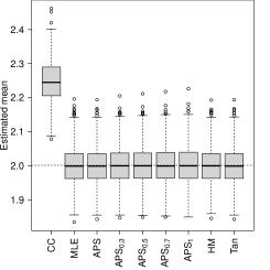
Model	Criteria	Method
		CC	MLE	APS	${\rm APS}_{0.3}$	${\rm APS}_{0.5}$	${\rm APS}_{0.7}$	${\rm APS}_{1}$	HM	Tan
OM1PM1	Bias	2.45	-0.01	-0.01	-0.01	-0.01	-0.01	-0.01	-0.01	-0.01
	S.E.	0.61	0.56	0.55	0.56	0.56	0.57	0.58	0.55	0.55
	RMSE	2.53	0.56	0.55	0.56	0.56	0.57	0.58	0.55	0.55
OM2PM1	Bias	4.03	0.06	0.10	0.68	0.72	0.74	0.76	0.13	0.11
	S.E.	2.54	3.10	2.97	1.66	1.65	1.65	1.66	2.44	2.95
	RMSE	4.77	3.10	2.97	1.79	1.80	1.81	1.82	2.45	2.95
OM1PM2	Bias	3.07	-0.29	-0.00	-0.00	-0.00	-0.00	-0.00	-0.00	-0.00
	S.E.	0.61	0.59	0.55	0.56	0.56	0.57	0.58	0.55	0.55
	RMSE	3.13	0.66	0.55	0.56	0.56	0.57	0.58	0.55	0.55
OM2PM2	Bias	3.14	-4.67	-3.22	-0.78	-0.63	-0.56	-0.51	-2.45	-3.16
	S.E.	2.59	6.45	4.42	1.73	1.71	1.71	1.70	3.25	4.30
	RMSE	4.07	7.96	5.47	1.89	1.82	1.79	1.78	4.07	5.33

(a) OM1PM1

(b) OM2PM1

(c) OM1PM2

(d) OM2PM2

Figure 2: Boxplots for estimators comparison with sample size $1000$ and Monte Carlo sample $1000$; 20% of the samples are contaminated with the additive noise from $Unif(-50,50)$. The errors from outcome models are generated from i.i.d. standard Gaussian distribution. CC: mean of the complete cases; MLE: maximum likelihood estimation; APS: augmented propensity score weighting estimator; $\mathrm{APS}_{\gamma}$: augmented propensity score weighting with $\gamma$-divergence estimator, for $\gamma=0.3,0.5,0.7,1$; HM: entropy balancing method in Hainmueller, (2012); Tan: regularized calibration method in Tan, (2019).

Table 2: Bias, standard error (S.E.), root mean square error (RMSE) for estimators comparison with sample size $1000$ and Monte Carlo sample $1000$; 20% of the samples are contaminated with the additive noise from $Unif(-50,50)$. The errors from outcome models are generated from i.i.d. standard Gaussian distribution. All criteria are multiplied by 10. CC: mean of the complete cases; MLE: maximum likelihood estimation; APS: augmented propensity score weighting estimator; $\mathrm{APS}_{\gamma}$: augmented propensity score weighting with $\gamma$-divergence estimator, for $\gamma=0.3,0.5,0.7,1$; HM: entropy balancing method in Hainmueller, (2012); Tan: regularized calibration method in Tan, (2019)

Model	Criteria	Method
		CC	MLE	APS	${\rm APS}_{0.3}$	${\rm APS}_{0.5}$	${\rm APS}_{0.7}$	${\rm APS}_{1}$	HM	Tan
OM1PM1	Bias	2.28	-0.21	-0.21	-0.12	-0.12	-0.12	-0.12	-0.21	-0.19
	S.E.	5.12	5.31	5.31	3.13	3.13	3.13	3.13	5.27	5.31
	RMSE	5.60	5.31	5.31	3.13	3.13	3.13	3.13	5.27	5.31
OM2PM1	Bias	3.86	-0.14	-0.10	0.57	0.62	0.64	0.66	-0.07	-0.07
	S.E.	5.63	6.03	5.96	3.46	3.46	3.46	3.47	5.70	5.96
	RMSE	6.82	6.03	5.96	3.51	3.52	3.52	3.53	5.70	5.95
OM1PM2	Bias	2.92	-0.51	-0.21	-0.09	-0.09	-0.09	-0.09	-0.20	-0.18
	S.E.	5.17	5.70	5.51	3.13	3.13	3.13	3.13	5.43	5.50
	RMSE	5.93	5.72	5.51	3.13	3.13	3.13	3.13	5.43	5.50
OM2PM2	Bias	3.00	-4.89	-3.42	-0.79	-0.71	-0.65	-0.59	-2.65	-3.35
	S.E.	5.69	8.27	6.81	3.42	3.48	3.49	3.48	6.14	6.75
	RMSE	6.43	9.61	7.62	3.50	3.55	3.55	3.53	6.68	7.54

Table 3: Linearized variance estimation for gamma divergence method where the errors are i.i.d. from standard Gaussian distribution

Model	Coverage rate	Method
		$\rm{APS}_{0.3}$	$\rm{APS}_{0.5}$	$\rm{APS}_{0.7}$	$\rm{APS}_{1.0}$
OM1RM1	$90\%$	89.9 %	89.8 %	90.1 %	89.7 %
	$95\%$	95.1 %	94.5 %	94.3 %	94.3 %
OM1RM2	$90\%$	90.1 %	90.3 %	90.4 %	90.4 %
	$95\%$	95.2 %	95.0 %	94.7 %	94.6 %

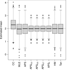
Figure 1 shows the results of the simulation study above, where the dashed line represents the true parameter $\theta=E(Y)$. Table 1 presents the corresponding bias, standard error, and root mean square error for each method. Since the consistency of all estimators is guaranteed under OM1PM1, we can see that all estimators give similar performances except for the mean of the complete cases method. However, under OM1PM2, the consistency of the generalized linear model method is no longer guaranteed, while that of other estimators is still valid. In OM1PM2, the covariate balancing condition becomes critical, and so all methods satisfying the covariate balancing will be unbiased. In OM2PM1, the proposed augmented PSW estimator is still consistent, as the propensity score model is correctly specified. Our proposed augmented PSW estimator with $\gamma$-divergence is biased in this scenario due to the misspecification of the outcome model, where other estimators are built under the correct specified response model. In OM2PM2, all estimators present some deviations from the true mean of $y_{i}^{\prime}s$. However, our proposed augmented PSW estimator with $\gamma$-divergence is robust against other estimators, with fewer outliers and the smallest root mean square error.

We also investigated the performance of the proposed linearization variance estimator in (43). We computed confidence intervals based on asymptotic normality. The results are presented in Table 3. The performances are satisfactory when the ourcome regression model is specified correctly.

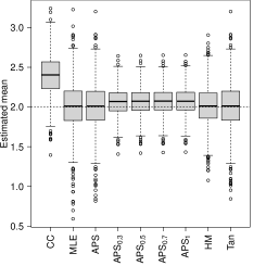
In addition, we check the robustness of the augmented propensity score weighting estimator with $\gamma$-divergence against outliers. After the data are generated under the same $2\times 2$ factorial design as in the previous simulation setting, additional noise generated from ${Uinf}(-50,50)$ is added to 20% of the observed outcomes. Again, the sample size is $1,000$ and the Monte Carlo sample size is $1,000$.

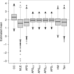
Figure 2 shows the performance of various estimators, where the dashed line represents the true mean of $y_{i}^{\prime}s$. Table 2 presents the corresponding bias, standard error, and root mean square error for each method. Compared to other estimators, in all four scenarios, our proposed augmented propensity score weighting estimator with $\gamma$-divergence apparently gives the smallest root mean square error, which validates our robustness claim in Section 4.

6.2 Real data application

We further check our proposed estimators for artificial missingness with real data from the California API program (http://api.cde.ca.gov/ or survey package (Lumley,, 2010) in R (R Core Team,, 2022)). Within the data set, standardized student tests are performed to calculate the API for California schools. Specifically, we select the API for year 2000 (api00) as the response variable. For covariates, we set the API for year 1999 (api99) as $x_{1}$, the percentage of students eligible for subsidized meals (meals) as $x_{2}$, the percentage of English language learners (ell) as $x_{3}$, the average level of parental education (avg) as $x_{4}$, the percentage of fully qualified teachers (full) as $x_{5}$, and the number of students enrolled (enroll) as $x_{6}$, where the words in parentheses are the abbreviations for variable names in the dataset. We artificially created the missingness with the following two response mechanisms: PM3, where $\delta\mid{\boldsymbol{x}}$ follows the Bernoulli distribution with $\mathrm{logit}\{P(\delta=1\mid{\boldsymbol{x}})\}=\phi_{0}+2x_{1}+x_{2}+0.5x_{3},$ and $\phi_{0}$ is chosen to achieve the 60% response rates; PM4, where $\delta\mid{\boldsymbol{x}}$ follows the Bernoulli distribution with ${P}(\delta=1\mid{\boldsymbol{x}})=0.8$, if $a+2x_{1}+x_{2}+x_{3}+x_{4}+x_{5}+x_{6}>0$, ${P}(\delta=1\mid{\boldsymbol{x}})=0.4$ otherwise, and $a$ is chosen to achieve the response rates 60%.

(a) PM3

(b) PM4

Figure 3: Estimators comparison in real data with $1000$ Monte Carlo sample, with artificially missingness mechanism PM3 and PM4. APS: augmented propensity score weighting estimator; $\mathrm{APS}_{\gamma}$: augmented propensity score weighting with $\gamma$-divergence estimator, where $\gamma$ is chosen by the cross-validation method based on MSPE criterion; MLE: maximum likelihood estimation; HM: entropy balancing method in Hainmueller, (2012); Tan: regularized calibration method in Tan, (2019).

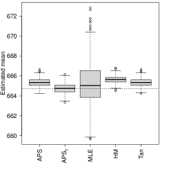
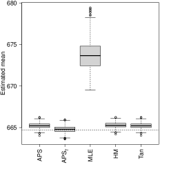
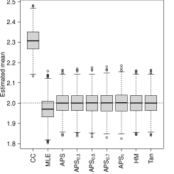
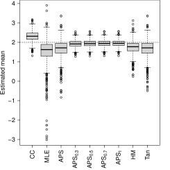
We compare the same estimators as in previous subsections with 1000 Monte Carlo samples. In particular, the mean of the complete cases method does not behave well in both cases and will affect the scale of the resultant box plots, so we do not show its performance. Furthermore, we adopt the MSPE as the 5-fold cross-validation criterion for the selection strategy of $\gamma$, as described in Section 4. For each Monte Carlo sample, we select the best $\gamma$ from $\{0.1,0.2,\ldots,1\}$ and denote the corresponding estimator as ${\mathrm{APS}}_{\gamma}$. The results are summarized with box plots in Figure 3, where the dashed line denotes the true population mean. As we can see, the estimator ${\mathrm{APS}}_{\gamma}$ always gives the unbiased estimate with a relatively low root mean square error, outperforming other estimators.

7 Application to CEAP data

The Conservation Effects Assessment Project (CEAP) is a program initiated by the United States Department of Agriculture (USDA) Natural Resources Conservation Service (NRCS). CEAP collects and analyzes data from various sources, including field studies, monitoring sites, and modeling, to evaluate the impact of water and wind erosion. Further details of the CEAP data can be found in Berg and Yu, (2019). The farmer’s interview data together with the NRI data serve as input to the revised Universal Soil Loss Equation (RUSLE2) to generate a measure of sheet and rill erosion. In addition, RUSLE2 is also an advancement of a traditional approximation called the Universal Soil Loss Equation (USLE). For the CEAP sample, the RUSLE2 suffers from missingness due to the refuse of the farmer interviewed, while the corresponding USLE is available.

(a) Normal Q-Q plot

(b) Mean estimation

Figure 4: Quantile-quantile plot and mean estimation with 95% confidence band for CEAP data in Arkansas.

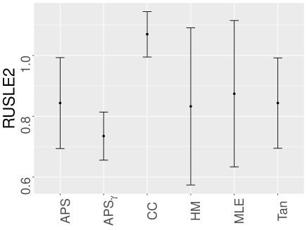
We are interested in estimating the population mean of RUSLE2 using USLE as an auxiliary variable for calibration weighting in Arkansas. Specifically, the total sampled points are 1509 and the fully observed are 406, with observed rate $26.9\%$. The normal quantile-quantile (Q-Q) plot generated from linear models based on the complete cases is presented in Sub-figure (a) of Figure 4. By the normal Q-Q plot, numerous outlier data points are evident, and the residuals deviate from satisfying the assumption of a normal distribution. Therefore, given this scenario, we have strong reasons to place greater trust in our suggested robust approach. The associated mean estimation result is presented in Sub-figure (b) of Figure 4. In this presentation, our proposed method using gamma divergence exhibits a narrow 95% confidence interval and yields a low RUSLE2 value.

8 Concluding Remarks

We have applied the information projection is applied to obtain an augmented PS model that allows for doubly robust estimation. We have introduced self-efficiency to obtain the equivalence between the PSW estimator and the regression imputation estimator. In addition, $\gamma$-power divergence can be used to obtain an outlier-robust regression imputation estimator. By imposing self-efficiency, the resulting PSW estimator is also robust to outliers. In practice, an efficient and outlier-robust PSW estimator is very attractive as the existence of outliers can often damage the efficiency of the result estimator.

There are several directions of further extensions of the proposed method. The proposed method is directly applicable to the calibration weighting in survey sampling (Fuller,, 2009; Tillé,, 2020). The proposed method is based on the assumption of missing at random. Extension to nonignorable nonresponse can also be an interesting research direction.

Appendix

Appendix A Proof of main theorems

Proof of Lemma 3

If the balancing condition (3) holds, then the propensity score weighting estimator can be expressed as

$$\hat{\theta}_{\rm{PSW}} = \frac{1}{n}\sum_{i=1}^{n}\delta_{i}\omega_{i}y_{i}$$

$$= \frac{1}{n}\sum_{i=1}^{n}\delta_{i}\omega_{i}\left(m_{i}+\varepsilon_{i}\right)$$

$$= \frac{1}{n}\sum_{i=1}^{n}\delta_{i}\omega_{i}m_{i}+\frac{1}{n}\sum_{i=1}^{n}\delta_{i}\omega_{i}\varepsilon_{i}$$

$$= \frac{1}{n}\sum_{i=1}^{n}m_{i}+\frac{1}{n}\sum_{i=1}^{n}\delta_{i}\omega_{i}\varepsilon_{i},$$

where $m_{i}=m(\boldsymbol{x}_{i};\boldsymbol{\beta})$. Then

$$\hat{\theta}_{\rm PSW}-\hat{\theta}_{\rm{com}}=\frac{1}{n}\sum_{i=1}^{n}\left(\delta_{i}\omega_{i}-1\right)\varepsilon_{i}.$$

Under the MAR assumption, we can obtain

$$E\left(\hat{\theta}_{\rm PSW}-\hat{\theta}_{\rm{com}}\mid\boldsymbol{x}_{1},\ldots,\boldsymbol{x}_{n},\boldsymbol{\delta}\right)=\frac{1}{n}\sum_{i=1}^{n}\left(\delta_{i}\omega_{i}-1\right)E(\varepsilon_{i}\mid\boldsymbol{x}_{i})=0.$$

Thus, we can conclude that $\hat{\theta}_{\rm PS}$ is unbiased for $\theta$.

Proof of Lemma 6

Note that we can express the indirect model calibration condition (3) as

$$\sum_{i=1}^{n}\left(1-\delta_{i}\omega_{i}\right)\boldsymbol{{b}}_{i}=\mathbf{0}.$$ (49)

Thus, as long as (49) is satisfied, we can write

$$\hat{\theta}_{\rm PSW} = n^{-1}\sum_{i=1}^{n}\delta_{i}\omega_{i}y_{i}+n^{-1}\sum_{i=1}^{n}\left(1-\delta_{i}\omega_{i}\right)\boldsymbol{{b}}_{i}^{\operatorname{T}}\boldsymbol{\beta}$$

$$= n^{-1}\sum_{i=1}^{n}\left\{\delta_{i}y_{i}+(1-\delta_{i})\boldsymbol{{b}}_{i}^{\operatorname{T}}\boldsymbol{\beta}\right\}+n^{-1}\sum_{i=1}^{n}\delta_{i}(\omega_{i}-1)(y_{i}-\boldsymbol{{b}}_{i}^{\operatorname{T}}\boldsymbol{\beta})$$

for any $\boldsymbol{\beta}$. Thus, as long as (6) hold, we can obtain (5).

Regularity Conditions for Theorem 28

Assumption 1.

Assume that there exists constants $C_{1}$ and $C_{2}$ such that

$$0<C_{1}\leq\lambda_{\rm{min}}\left(\frac{1}{n}\sum_{i=1}^{n}\boldsymbol{{b}}_{i}\boldsymbol{{b}}_{i}^{\rm T}\right)\leq\lambda_{\rm{max}}\left(\frac{1}{n}\sum_{i=1}^{n}\boldsymbol{{b}}_{i}\boldsymbol{{b}}_{i}^{\rm T}\right)\leq C_{2}<\infty,$$

where $\lambda_{\rm min}$ and $\lambda_{\rm max}$ are the smallest and largest eigenvalues of a specific matrix, respectively.

Assumption 2.

The estimating equation $\hat{\boldsymbol{U}}_{1}(\boldsymbol{\phi})=\mathbf{0}$ has a unique solution $\hat{\boldsymbol{\phi}}$ and $E\{\hat{\boldsymbol{U}}_{1}(\boldsymbol{\phi})\}=\mathbf{0}$ has a unique solution $\boldsymbol{\phi}^{\ast}$. Further, $\hat{\boldsymbol{U}}_{2}(\boldsymbol{\lambda}\mid\boldsymbol{\phi}^{\ast})=\mathbf{0}$ has a unique solution $\hat{\boldsymbol{\lambda}}$ and $E\{\hat{\boldsymbol{U}}_{2}(\boldsymbol{\lambda}\mid\boldsymbol{\phi}^{\ast})\}=\mathbf{0}$ has a unique solution $\boldsymbol{\lambda}^{\ast}$.

Assumption 3.

The estimating equation $\hat{\boldsymbol{U}}_{1}(\boldsymbol{\phi})$ converges to $E\{\hat{\boldsymbol{U}}_{1}(\boldsymbol{\phi})\}$ on a compact set $\mathcal{G}_{1}$ containing $\boldsymbol{\phi}^{\ast}$. In addition, $\hat{\boldsymbol{U}}_{2}(\boldsymbol{\lambda}\mid\boldsymbol{\phi}^{\ast})$ converges to $E\{\hat{\boldsymbol{U}}_{2}(\boldsymbol{\lambda}\mid\boldsymbol{\phi}^{\ast})\}$ on a compact set $\mathcal{G}_{2}$ containing $\boldsymbol{\lambda}^{\ast}$.

Assumption 4.

The matrices $E\{\partial_{\boldsymbol{\lambda}}\hat{\boldsymbol{U}}_{1}(\boldsymbol{\phi})\mid_{\boldsymbol{\phi}=\boldsymbol{\phi}^{\star}}\}$ and $E\{\partial_{\boldsymbol{\lambda}}\hat{\boldsymbol{U}}_{2}(\boldsymbol{\lambda}\mid\boldsymbol{\phi}^{\ast})\mid_{\boldsymbol{\lambda}=\boldsymbol{\lambda}^{\ast}}\}$ are both nonsingular.

Proof of Theorem 28

Since $\hat{\boldsymbol{\lambda}}$ satisfies (23), we can obtain the following equivalence

$$\hat{\theta}_{\rm APSW} = \frac{1}{n}\sum_{i=1}^{n}\delta_{i}\omega^{*}(\boldsymbol{x}_{i};\hat{\boldsymbol{\phi}},\hat{\boldsymbol{\lambda}})y_{i}-\hat{\boldsymbol{U}}_{2}^{\operatorname{T}}(\hat{\boldsymbol{\lambda}}\mid\hat{\boldsymbol{\phi}})\boldsymbol{\beta}$$

$$= \frac{1}{n}\sum_{i=1}^{n}\left\{\boldsymbol{{b}}_{i}^{\operatorname{T}}\boldsymbol{\beta}+\delta_{i}\omega^{*}(\boldsymbol{x}_{i};\hat{\boldsymbol{\phi}},\hat{\boldsymbol{\lambda}})(y_{i}-\boldsymbol{{b}}_{i}^{\operatorname{T}}\boldsymbol{\beta})\right\}$$

$$:= \hat{\theta}_{\rm APSW}(\hat{\boldsymbol{\lambda}};\boldsymbol{\beta})$$

for any $\boldsymbol{\beta}$. Now,

$$\frac{\partial}{\partial\boldsymbol{\lambda}}\hat{\theta}_{\rm APSW}(\boldsymbol{\lambda};\boldsymbol{\beta}) = \frac{1}{n}\sum_{i=1}^{n}\delta_{i}\left(\hat{\pi}_{i}^{-1}-1\right)\exp\left(\boldsymbol{{b}}_{i}^{\operatorname{T}}\boldsymbol{\lambda}\right)\left(y_{i}-\boldsymbol{{b}}_{i}^{\operatorname{T}}\boldsymbol{\beta}\right)\boldsymbol{{b}}_{i}.$$

Thus, for the choice of $\hat{\boldsymbol{\beta}}$ in (18), we can obtain

$$E\left\{\frac{\partial}{\partial\boldsymbol{\lambda}}\hat{\theta}_{\rm APSW}(\boldsymbol{\lambda};{\boldsymbol{\beta}}^{*})\right\}=\boldsymbol{0}.$$

Thus, the uncertainty associated with $\hat{\boldsymbol{\lambda}}$ is asymptotically negligible at $\boldsymbol{\beta}=\boldsymbol{\beta}^{*}$. Thus, we obtain

$$\hat{\theta}_{\rm{APSW}}(\boldsymbol{\lambda}^{\ast};\boldsymbol{\beta}^{\ast})=\frac{1}{n}\sum_{i=1}^{n}\left\{\boldsymbol{{b}}_{i}^{\operatorname{T}}{\boldsymbol{\beta}}^{*}+\delta_{i}\hat{\omega}^{*}(\boldsymbol{x}_{i};\hat{\boldsymbol{\phi}},\boldsymbol{\lambda}^{*})(y_{i}-\boldsymbol{{b}}_{i}^{\operatorname{T}}{\boldsymbol{\beta}}^{*})\right\}+o_{p}(n^{-1/2}).$$ (50)

Now, to apply Taylor linearization with respect to $\boldsymbol{\phi}$, we define

$$\hat{\theta}_{\ell}(\hat{\boldsymbol{\phi}};\boldsymbol{\kappa}) \equiv \frac{1}{n}\sum_{i=1}^{n}\left\{\boldsymbol{{b}}_{i}^{\operatorname{T}}{\boldsymbol{\beta}}^{*}+\delta_{i}\hat{\omega}^{*}(\boldsymbol{x}_{i};\hat{\boldsymbol{\phi}},\boldsymbol{\lambda}^{*})(y_{i}-\boldsymbol{{b}}_{i}^{\operatorname{T}}{\boldsymbol{\beta}}^{*})\right\}-\hat{\boldsymbol{U}}_{1}^{\operatorname{T}}(\hat{\boldsymbol{\phi}})\boldsymbol{\kappa}$$

$$= \frac{1}{n}\sum_{i=1}^{n}\left[\delta_{i}y_{i}+(1-\delta_{i})\left(\boldsymbol{{b}}_{i}^{\operatorname{T}}{\boldsymbol{\beta}}^{*}+\bm{h}_{i}^{\operatorname{T}}\boldsymbol{\kappa}\right)+\delta_{i}\left(\hat{\pi}_{i}^{-1}-1\right)\left\{\exp(\boldsymbol{{b}}_{i}^{\operatorname{T}}\boldsymbol{\lambda}^{*})(y_{i}-\boldsymbol{{b}}_{i}^{\operatorname{T}}{\boldsymbol{\beta}}^{*})-\bm{h}_{i}^{\operatorname{T}}\boldsymbol{\kappa}\right\}\right].$$

Then,

$$\frac{\partial}{\partial\boldsymbol{\phi}}\hat{\theta}_{\ell}({\boldsymbol{\phi}};\boldsymbol{\kappa})\Big{|}_{\boldsymbol{\phi}=\boldsymbol{\phi}^{\ast}}=\frac{1}{n}\sum_{i=1}^{n}\delta_{i}\left\{\frac{1}{\pi_{0}(\boldsymbol{x}_{i};\boldsymbol{\phi}^{*})}-1\right\}\left\{\exp(\boldsymbol{{b}}_{i}^{\operatorname{T}}\boldsymbol{\lambda}^{*})(y_{i}-\boldsymbol{{b}}_{i}^{\operatorname{T}}{\boldsymbol{\beta}}^{*})-\bm{h}_{i}^{\operatorname{T}}\boldsymbol{\kappa}\right\}\frac{\partial}{\partial\boldsymbol{\phi}}\pi_{0}(\boldsymbol{x}_{i};\boldsymbol{\phi})\Big{|}_{\boldsymbol{\phi}=\boldsymbol{\phi}^{\ast}}.$$

Thus, we can choose $\boldsymbol{\kappa}^{*}$ to satisfy

$$E\left\{\frac{\partial}{\partial\boldsymbol{\phi}}\hat{\theta}_{\ell}({\boldsymbol{\phi}};\boldsymbol{\kappa}^{*})\Big{|}_{\boldsymbol{\phi}=\boldsymbol{\phi}^{\ast}}\right\}=\mathbf{0},$$

which gives the final linearization form as in (26).

Regularity Conditions for Theorem 4.1

Define

$$\hat{\boldsymbol{U}}_{3}(\boldsymbol{\lambda},\boldsymbol{\beta},\sigma^{2}\mid\boldsymbol{\phi}^{\ast})=\begin{pmatrix}\frac{1}{n}\left[\sum_{i=1}^{n}\delta_{i}\left\{1+\{d_{i}(\boldsymbol{\phi}^{\ast})-1\}g_{i}(\boldsymbol{\lambda})q_{\gamma,i}(\boldsymbol{\beta},\sigma^{2})\right\}\boldsymbol{{b}}_{i}-\sum_{i=1}^{n}\boldsymbol{{b}}_{i}\right]\\ \frac{1}{n}\sum_{i=1}^{n}\delta_{i}\{d_{i}(\boldsymbol{\phi}^{\ast})-1\}g_{i}(\boldsymbol{\lambda})q_{\gamma,i}(\boldsymbol{\beta},\sigma^{2})(y_{i}-\boldsymbol{{b}}_{i}^{\rm T}\boldsymbol{\beta})\boldsymbol{{b}}_{i}\\ \frac{1}{n}\sum_{i=1}^{n}\delta_{i}\{d_{i}(\boldsymbol{\phi}^{\ast})-1\}g_{i}(\boldsymbol{\lambda})q_{\gamma,i}(\boldsymbol{\beta},\sigma^{2})(y_{i}-\boldsymbol{{b}}_{i}^{\rm T}\boldsymbol{\beta})^{2}\left\{(y_{i}-\boldsymbol{{b}}_{i}^{\rm T}\boldsymbol{\beta})^{2}-\frac{\sigma^{2}}{1+\gamma}\right\}\end{pmatrix}.$$ (51)

In addition with the regularity conditions in Theorem 4.1, we need the following additional assumptions.

Assumption 5.

Assume that there exists constants $C_{3}$ and $C_{4}$ such that

$$0<C_{3} \leq\lambda_{\rm{min}}\left(\frac{1}{n}\sum_{i=1}^{n}\delta_{i}\{d_{i}(\boldsymbol{\phi}^{\ast})-1\}g_{i}(\boldsymbol{\lambda}^{\ast})q_{\gamma_{i}}(\boldsymbol{\beta}^{\ast},\sigma^{\ast 2})\boldsymbol{{b}}_{i}\boldsymbol{{b}}_{i}^{\rm T}\right)$$

$$\leq\lambda_{\rm{max}}\left(\frac{1}{n}\sum_{i=1}^{n}\delta_{i}\{d_{i}(\boldsymbol{\phi}^{\ast})-1\}g_{i}(\boldsymbol{\lambda}^{\ast})q_{\gamma_{i}}(\boldsymbol{\beta}^{\ast},\sigma^{\ast 2})\boldsymbol{{b}}_{i}\boldsymbol{{b}}_{i}^{\rm T}\right)\leq C_{4}<\infty.$$

Assumption 6.

The estimating equation $\hat{\boldsymbol{U}}_{3}(\boldsymbol{\lambda},\boldsymbol{\beta},\sigma^{2}\mid\boldsymbol{\phi}^{\ast})=\mathbf{0}$ has a unique solution $(\hat{\boldsymbol{\lambda}},\hat{\boldsymbol{\beta}}_{q},\hat{\sigma}_{q}^{2})$ and $E\{\hat{\boldsymbol{U}}_{3}(\boldsymbol{\lambda},\boldsymbol{\beta},\sigma^{2}\mid\boldsymbol{\phi}^{\ast})\}=\mathbf{0}$ has a unique solution $(\boldsymbol{\lambda}^{\ast},\boldsymbol{\beta}^{\ast},\sigma^{\ast 2})$.

Assumption 7.

The estimating equation $\hat{\boldsymbol{U}}_{3}(\boldsymbol{\lambda},\boldsymbol{\beta},\sigma^{2}\mid\boldsymbol{\phi}^{\ast})$ converges to $E\{\hat{\boldsymbol{U}}_{3}(\boldsymbol{\lambda},\boldsymbol{\beta},\sigma^{2}\mid\boldsymbol{\phi}^{\ast})\}$ on a compact set $\mathcal{G}_{3}$ containing $(\boldsymbol{\lambda}^{\ast},\boldsymbol{\beta}^{\ast},\sigma^{\ast 2})$.

Assumption 8.

The matrix $E\{\partial_{(\boldsymbol{\lambda}^{\rm T},\boldsymbol{\beta}^{\rm T},\sigma^{2})^{\rm T}}\hat{\boldsymbol{U}}_{3}(\boldsymbol{\lambda},\boldsymbol{\beta},\sigma^{2}\mid\boldsymbol{\phi}^{\ast})\mid_{\boldsymbol{\lambda}=\boldsymbol{\lambda}^{\ast},\boldsymbol{\beta}=\boldsymbol{\beta}^{\ast},\sigma^{2}=\sigma^{\ast 2}}\}$ is nonsingular.

Proof of Theorem 4.1

By the normal equations, we have

$$\theta_{\rm APSW,\gamma}(\hat{\boldsymbol{\lambda}},\hat{\boldsymbol{\beta}}_{q},\hat{\sigma}_{q}^{2}\mid\hat{\boldsymbol{\phi}};\boldsymbol{\mu},\boldsymbol{\zeta},\nu)$$

$$= \frac{1}{n}\sum_{i=1}^{n}\delta_{i}\omega_{\gamma,i}(\boldsymbol{x}_{i};\hat{\boldsymbol{\lambda}},\hat{\boldsymbol{\beta}}_{q},\hat{\sigma}_{q}^{2},\hat{\boldsymbol{\phi}})y_{i}-\frac{\boldsymbol{\mu}^{\rm T}}{n}\left[\sum_{i=1}^{n}\delta_{i}\left\{1+\{d_{i}(\hat{\boldsymbol{\phi}})-1\}g_{i}(\hat{\boldsymbol{\lambda}})q_{\gamma,i}(\hat{\boldsymbol{\beta}}_{q},\hat{\sigma}_{q}^{2})\right\}\boldsymbol{{b}}_{i}-\sum_{i=1}^{n}\boldsymbol{{b}}_{i}\right]$$

$$\quad+\frac{\boldsymbol{\zeta}^{\rm T}}{n}\sum_{i=1}^{n}\delta_{i}\{d_{i}(\hat{\boldsymbol{\phi}})-1\}g_{i}(\hat{\boldsymbol{\lambda}})q_{\gamma,i}(\hat{\boldsymbol{\beta}}_{q},\hat{\sigma}_{q}^{2})(y_{i}-\boldsymbol{{b}}_{i}^{\rm T}\hat{\boldsymbol{\beta}}_{q})\boldsymbol{{b}}_{i}$$

$$\quad+\frac{\nu}{n}\sum_{i=1}^{n}\delta_{i}\{d_{i}(\hat{\boldsymbol{\phi}})-1\}g_{i}(\hat{\boldsymbol{\lambda}})q_{\gamma,i}(\hat{\boldsymbol{\beta}}_{q},\hat{\sigma}_{q}^{2})(y_{i}-\boldsymbol{{b}}_{i}^{\rm T}\hat{\boldsymbol{\beta}}_{q})^{2}\left\{(y_{i}-\boldsymbol{{b}}_{i}^{\rm T}\hat{\boldsymbol{\beta}}_{q})^{2}-\frac{\hat{\sigma}_{q}^{2}}{1+\gamma}\right\}$$

$$= \frac{1}{n}\sum_{i=1}^{n}\boldsymbol{{b}}_{i}^{\rm T}\boldsymbol{\mu}+\frac{1}{n}\sum_{i=1}^{n}\delta_{i}\omega_{\gamma,i}(\boldsymbol{x}_{i};\hat{\boldsymbol{\lambda}},\hat{\boldsymbol{\beta}}_{q},\hat{\sigma}_{q}^{2},\hat{\boldsymbol{\phi}})(y_{i}-\boldsymbol{{b}}_{i}^{\rm T}\boldsymbol{\mu})$$

$$\quad+\frac{\boldsymbol{\zeta}^{\rm T}}{n}\sum_{i=1}^{n}\delta_{i}\{d_{i}(\hat{\boldsymbol{\phi}})-1\}g_{i}(\hat{\boldsymbol{\lambda}})q_{\gamma,i}(\hat{\boldsymbol{\beta}}_{q},\hat{\sigma}_{q}^{2})(y_{i}-\boldsymbol{{b}}_{i}^{\rm T}\hat{\boldsymbol{\beta}}_{q})\boldsymbol{{b}}_{i}$$

$$\quad+\frac{\nu}{n}\sum_{i=1}^{n}\delta_{i}\{d_{i}(\hat{\boldsymbol{\phi}})-1\}g_{i}(\hat{\boldsymbol{\lambda}})q_{\gamma,i}(\hat{\boldsymbol{\beta}}_{q},\hat{\sigma}_{q}^{2})(y_{i}-\boldsymbol{{b}}_{i}^{\rm T}\hat{\boldsymbol{\beta}}_{q})^{2}\left\{(y_{i}-\boldsymbol{{b}}_{i}^{\rm T}\hat{\boldsymbol{\beta}}_{q})^{2}-\frac{\hat{\sigma}_{q}^{2}}{1+\gamma}\right\}$$ (52)

for any $\boldsymbol{\mu}\in\mathbb{R}^{p}$, $\boldsymbol{\zeta}\in\mathbb{R}^{p}$ and $\nu\in\mathbb{R}$. In addition, tedious derivation will lead

$$\begin{pmatrix}\frac{\partial}{\partial\boldsymbol{\lambda}}\theta_{\rm APSW,\gamma}(\boldsymbol{\beta},\sigma^{2},\boldsymbol{\lambda}\mid\hat{\boldsymbol{\phi}};\boldsymbol{\mu},\boldsymbol{\zeta},\nu)\\ \frac{\partial}{\partial\boldsymbol{\beta}}\theta_{\rm APSW,\gamma}(\boldsymbol{\beta},\sigma^{2},\boldsymbol{\lambda}\mid\hat{\boldsymbol{\phi}};\boldsymbol{\mu},\boldsymbol{\zeta},\nu)\\ \frac{\partial}{\partial\sigma^{2}}\theta_{\rm APSW,\gamma}(\boldsymbol{\beta},\sigma^{2},\boldsymbol{\lambda}\mid\hat{\boldsymbol{\phi}};\boldsymbol{\mu},\boldsymbol{\zeta},\nu)\end{pmatrix}=\frac{1}{n}\begin{pmatrix}\bm{s}_{10}+\bm{s}_{11}\boldsymbol{\mu}+\bm{s}_{12}\boldsymbol{\zeta}+\bm{s}_{13}\nu\\ s_{20}+\bm{s}_{21}\boldsymbol{\mu}+\bm{s}_{22}\boldsymbol{\zeta}+s_{23}\nu\\ \bm{s}_{30}+\bm{s}_{31}\boldsymbol{\mu}+\bm{s}_{32}\boldsymbol{\zeta}+\bm{s}_{33}\nu\end{pmatrix}$$ (53)

where

$$\bm{s}_{10}=\sum_{i=1}^{n}\delta_{i}\left\{\{d_{i}(\hat{\boldsymbol{\phi}})-1\}g_{i}(\boldsymbol{\lambda})q_{\gamma,i}(\boldsymbol{\beta},\sigma^{2})y_{i}\right\}\boldsymbol{{b}}_{i},$$

$$\bm{s}_{11}=-\sum_{i=1}^{n}\delta_{i}\left\{\{d_{i}(\hat{\boldsymbol{\phi}})-1\}g_{i}(\boldsymbol{\lambda})q_{\gamma,i}(\boldsymbol{\beta},\sigma^{2})\right\}\boldsymbol{{b}}_{i}\boldsymbol{{b}}_{i}^{\rm T},$$

$$\bm{s}_{12}=\sum_{i=1}^{n}\delta_{i}\{d_{i}(\hat{\boldsymbol{\phi}})-1\}g_{i}(\boldsymbol{\lambda})q_{\gamma,i}(\boldsymbol{\beta},\sigma^{2})(y_{i}-\boldsymbol{{b}}_{i}^{\rm T}\boldsymbol{\beta})\boldsymbol{{b}}_{i}\boldsymbol{{b}}_{i}^{\rm T},$$

$$\bm{s}_{13}=\sum_{i=1}^{n}\delta_{i}\{d_{i}(\hat{\boldsymbol{\phi}})-1\}g_{i}(\boldsymbol{\lambda})q_{\gamma,i}(\boldsymbol{\beta},\sigma^{2})(y_{i}-\boldsymbol{{b}}_{i}^{\rm T}\boldsymbol{\beta})^{2}\left\{(y_{i}-\boldsymbol{{b}}_{i}^{\rm T}\boldsymbol{\beta})^{2}-\frac{\sigma^{2}}{1+\gamma}\right\}\boldsymbol{{b}}_{i},$$

$$\bm{s}_{20}=\sum_{i=1}^{n}\delta_{i}\{d_{i}(\hat{\boldsymbol{\phi}})-1\}g_{i}(\boldsymbol{\lambda})q_{\gamma,i}(\boldsymbol{\beta},\sigma^{2})\left\{\frac{\gamma}{\sigma^{2}}(y_{i}-\boldsymbol{{b}}_{i}^{\rm T}\boldsymbol{\beta})\right\}y_{i}\boldsymbol{{b}}_{i},$$

$$\bm{s}_{21}=-\sum_{i=1}^{n}\delta_{i}\{d_{i}(\hat{\boldsymbol{\phi}})-1\}g_{i}(\boldsymbol{\lambda})q_{\gamma,i}(\boldsymbol{\beta},\sigma^{2})\left\{\frac{\gamma}{\sigma^{2}}(y_{i}-\boldsymbol{{b}}_{i}^{\rm T}\boldsymbol{\beta})\right\}\boldsymbol{{b}}_{i}\boldsymbol{{b}}_{i}^{\rm T},$$

$$\bm{s}_{22}=\sum_{i=1}^{n}\delta_{i}\{d_{i}(\hat{\boldsymbol{\phi}})-1\}g_{i}(\boldsymbol{\lambda})q_{\gamma,i}(\boldsymbol{\beta},\sigma^{2})\left\{\frac{\gamma}{\sigma^{2}}(y_{i}-\boldsymbol{{b}}_{i}^{\rm T}\boldsymbol{\beta})^{2}-1\right\}\boldsymbol{{b}}_{i}\boldsymbol{{b}}_{i}^{\rm T},$$

$$\bm{s}_{23}=\sum_{i=1}^{n}\delta_{i}\{d_{i}(\hat{\boldsymbol{\phi}})-1\}g_{i}(\boldsymbol{\lambda})q_{\gamma,i}(\boldsymbol{\beta},\sigma^{2})(y_{i}-\boldsymbol{{b}}_{i}^{\rm T}\boldsymbol{\beta})\left\{\frac{\gamma}{\sigma^{2}}(y_{i}-\boldsymbol{{b}}_{i}^{\rm T}\boldsymbol{\beta})^{2}-2\right\}\boldsymbol{{b}}_{i},$$

$$\bm{s}_{30}=\sum_{i=1}^{n}\delta_{i}\{d_{i}(\hat{\boldsymbol{\phi}})-1\}g_{i}(\boldsymbol{\lambda})q_{\gamma,i}(\boldsymbol{\beta},\sigma^{2})\frac{\gamma}{2(\sigma^{2})^{2}}(y_{i}-\boldsymbol{{b}}_{i}^{\rm T}\boldsymbol{\beta})^{2}y_{i},$$

$$\bm{s}_{31}=-\sum_{i=1}^{n}\delta_{i}\{d_{i}(\hat{\boldsymbol{\phi}})-1\}g_{i}(\boldsymbol{\lambda})q_{\gamma,i}(\boldsymbol{\beta},\sigma^{2})\frac{\gamma}{2(\sigma^{2})^{2}}(y_{i}-\boldsymbol{{b}}_{i}^{\rm T}\boldsymbol{\beta})^{2}\boldsymbol{{b}}_{i}^{\rm T},$$

$$\bm{s}_{32}=\sum_{i=1}^{n}\delta_{i}\{d_{i}(\hat{\boldsymbol{\phi}})-1\}g_{i}(\boldsymbol{\lambda})q_{\gamma,i}(\boldsymbol{\beta},\sigma^{2})\frac{\gamma}{2(\sigma^{2})^{2}}(y_{i}-\boldsymbol{{b}}_{i}^{\rm T}\boldsymbol{\beta})^{3}\boldsymbol{{b}}_{i}^{\rm T},$$

$$s_{33}=\sum_{i=1}^{n}\delta_{i}\{d_{i}(\hat{\boldsymbol{\phi}})-1\}g_{i}(\boldsymbol{\lambda})q_{\gamma,i}(\boldsymbol{\beta},\sigma^{2})\left[\frac{\gamma}{2(\sigma^{2})^{2}}(y_{i}-\boldsymbol{{b}}_{i}^{\rm T}\boldsymbol{\beta})^{2}\left\{(y_{i}-\boldsymbol{{b}}_{i}^{\rm T}\boldsymbol{\beta})^{2}-\frac{\sigma^{2}}{1+\gamma}\right\}-\frac{1}{1+\gamma}\right].$$

Therefore, we can choose $\boldsymbol{\mu}^{\ast}$, $\boldsymbol{\zeta}^{\ast}$ and $\nu^{\ast}$ such that

$$E\left\{\begin{pmatrix}\frac{\partial}{\partial\boldsymbol{\lambda}}\theta_{\rm APSW,\gamma}(\boldsymbol{\lambda},\boldsymbol{\beta},\sigma^{2}\mid\hat{\boldsymbol{\phi}};\boldsymbol{\mu}^{\ast},\boldsymbol{\zeta}^{\ast},\nu^{\ast})\\ \frac{\partial}{\partial\boldsymbol{\beta}}\theta_{\rm APSW,\gamma}(\boldsymbol{\lambda},\boldsymbol{\beta},\sigma^{2}\mid\hat{\boldsymbol{\phi}};\boldsymbol{\mu}^{\ast},\boldsymbol{\zeta}^{\ast},\nu^{\ast})\\ \frac{\partial}{\partial\sigma^{2}}\theta_{\rm APSW,\gamma}(\boldsymbol{\lambda},\boldsymbol{\beta},\sigma^{2}\mid\hat{\boldsymbol{\phi}};\boldsymbol{\mu}^{\ast},\boldsymbol{\zeta}^{\ast},\nu^{\ast})\end{pmatrix}\Bigg{|}_{\begin{subarray}{c}\boldsymbol{\lambda}=\boldsymbol{\lambda}^{\ast},\\ \boldsymbol{\beta}=\boldsymbol{\beta}^{\ast},\\ \sigma^{2}=\sigma^{\ast 2}\end{subarray}}\right\}=\mathbf{0},$$ (54)

where ensures that

$$\quad\theta_{\rm APSW,\gamma}(\boldsymbol{\lambda}^{\ast},{\boldsymbol{\beta}}^{\ast},\sigma^{\ast 2}\mid\hat{\boldsymbol{\phi}};\boldsymbol{\mu}^{\ast},\boldsymbol{\zeta}^{\ast},\nu^{\ast})$$

$$=\frac{1}{n}\sum_{i=1}^{n}\boldsymbol{{b}}_{i}^{\rm T}\boldsymbol{\mu}^{\ast}+\frac{1}{n}\sum_{i=1}^{n}\delta_{i}\omega_{\gamma,i}(\boldsymbol{x}_{i};\boldsymbol{\lambda}^{\ast},\boldsymbol{\beta}^{\ast},\sigma^{\ast 2},\hat{\boldsymbol{\phi}})(y_{i}-\boldsymbol{{b}}_{i}^{\rm T}\boldsymbol{\mu}^{\ast})$$

$$\quad+\frac{\boldsymbol{\zeta}^{\ast\rm{T}}}{n}\sum_{i=1}^{n}\delta_{i}\{d_{i}(\hat{\boldsymbol{\phi}})-1\}g_{i}(\boldsymbol{\lambda}^{\ast})q_{\gamma,i}(\boldsymbol{\beta}^{\ast},\sigma^{\ast 2})(y_{i}-\boldsymbol{{b}}_{i}^{\rm T}\boldsymbol{\beta}^{\ast})\boldsymbol{{b}}_{i}$$

$$\quad+\frac{\nu^{\ast}}{n}\sum_{i=1}^{n}\delta_{i}\{d_{i}(\hat{\boldsymbol{\phi}})-1\}g_{i}(\boldsymbol{\lambda}^{\ast})q_{\gamma,i}(\boldsymbol{\beta}^{\ast},\sigma^{\ast 2})(y_{i}-\boldsymbol{{b}}_{i}^{\rm T}\boldsymbol{\beta}^{\ast})^{2}\left\{(y_{i}-\boldsymbol{{b}}_{i}^{\rm T}\boldsymbol{\beta}^{\ast})^{2}-\frac{\sigma^{\ast 2}}{1+\gamma}\right\}$$

$$=\theta_{\rm APSW,\gamma}(\hat{\boldsymbol{\lambda}},\hat{\boldsymbol{\beta}}_{q},\hat{\sigma}_{q}^{2},\hat{\boldsymbol{\phi}})+o_{p}(n^{-1/2}).$$ (55)

Finally, we have

$$\quad\theta_{\rm APSW,\gamma}(\hat{\boldsymbol{\phi}}\mid\boldsymbol{\lambda}^{\ast},{\boldsymbol{\beta}}^{\ast},\sigma^{\ast 2};\boldsymbol{\mu}^{\ast},\boldsymbol{\zeta}^{\ast},\nu^{\ast},\boldsymbol{\kappa})$$

$$=\frac{1}{n}\sum_{i=1}^{n}\boldsymbol{{b}}_{i}^{\rm T}\boldsymbol{\mu}^{\ast}+\frac{1}{n}\sum_{i=1}^{n}\delta_{i}\omega_{\gamma,i}(\boldsymbol{x}_{i};\boldsymbol{\lambda}^{\ast},\boldsymbol{\beta}^{\ast},\sigma^{\ast 2},\hat{\boldsymbol{\phi}})(y_{i}-\boldsymbol{{b}}_{i}^{\rm T}\boldsymbol{\mu}^{\ast})$$

$$\quad+\frac{\boldsymbol{\zeta}^{\ast{\rm T}}}{n}\sum_{i=1}^{n}\delta_{i}\{d_{i}(\hat{\boldsymbol{\phi}})-1\}g_{i}(\boldsymbol{\lambda}^{\ast})q_{\gamma,i}(\boldsymbol{\beta}^{\ast},\sigma^{\ast 2})(y_{i}-\boldsymbol{{b}}_{i}^{\rm T}\boldsymbol{\beta}^{\ast})\boldsymbol{{b}}_{i}$$

$$\quad+\frac{\nu^{\ast}}{n}\sum_{i=1}^{n}\delta_{i}\{d_{i}(\hat{\boldsymbol{\phi}})-1\}g_{i}(\boldsymbol{\lambda}^{\ast})q_{\gamma,i}(\boldsymbol{\beta}^{\ast},\sigma^{\ast 2})(y_{i}-\boldsymbol{{b}}_{i}^{\rm T}\boldsymbol{\beta}^{\ast})^{2}\left\{(y_{i}-\boldsymbol{{b}}_{i}^{\rm T}\boldsymbol{\beta}^{\ast})^{2}-\frac{\sigma^{\ast 2}}{1+\gamma}\right\}$$

$$\quad-\hat{\boldsymbol{U}}_{1}^{\rm T}(\hat{\boldsymbol{\phi}})\boldsymbol{\kappa}$$ (56)

holds for any $\boldsymbol{\zeta}\in\mathbb{R}^{p}$. Apparently,

$$\quad\frac{\partial}{\partial\boldsymbol{\phi}}\theta_{\rm APSW,\gamma}(\boldsymbol{\phi}\mid\boldsymbol{\lambda}^{\ast},{\boldsymbol{\beta}}^{\ast},\sigma^{\ast 2};\boldsymbol{\mu}^{\ast},\boldsymbol{\zeta}^{\ast},\nu^{\ast},\boldsymbol{\kappa})$$

$$=-\frac{1}{n}\sum_{i=1}^{n}\delta_{i}d_{i}^{2}(\boldsymbol{\phi})g_{i}(\boldsymbol{\lambda})q_{\gamma,i}(\boldsymbol{\beta}^{\ast},\sigma^{\ast 2})(y_{i}-\boldsymbol{{b}}_{i}^{\rm T}\boldsymbol{\mu}^{\ast})\frac{\partial}{\partial\boldsymbol{\phi}}\pi(\boldsymbol{x}_{i},\boldsymbol{\phi})$$

$$\quad-\frac{1}{n}\sum_{i=1}^{n}\delta_{i}d_{i}^{2}(\boldsymbol{\phi})g_{i}(\boldsymbol{\lambda})q_{\gamma,i}(\boldsymbol{\beta}^{\ast},\sigma^{\ast 2})(y_{i}-\boldsymbol{{b}}_{i}^{\rm T}\boldsymbol{\beta}^{\ast})(\boldsymbol{\zeta}^{\ast{\rm T}}\boldsymbol{{b}}_{i})\frac{\partial}{\partial\boldsymbol{\phi}}\pi(\boldsymbol{x}_{i},\boldsymbol{\phi})$$

$$\quad-\frac{\nu^{\ast}}{n}\sum_{i=1}^{n}\delta_{i}d_{i}^{2}(\boldsymbol{\phi})g_{i}(\boldsymbol{\lambda})q_{\gamma,i}(\boldsymbol{\beta}^{\ast},\sigma^{\ast 2})(y_{i}-\boldsymbol{{b}}_{i}^{\rm T}\boldsymbol{\beta}^{\ast})^{2}\left\{(y_{i}-\boldsymbol{{b}}_{i}^{\rm T}\boldsymbol{\beta}^{\ast})^{2}-\frac{\sigma^{\ast 2}}{1+\gamma}\right\}\frac{\partial}{\partial\boldsymbol{\phi}}\pi(\boldsymbol{x}_{i},\boldsymbol{\phi})$$

$$\quad-\frac{1}{n}\sum_{i=1}^{n}\left[\left\{\delta_{i}d_{i}(\boldsymbol{\phi})-1\right\}\frac{\partial\bm{h}(\boldsymbol{x}_{i};\boldsymbol{\phi})}{\partial\boldsymbol{\phi}}-\delta_{i}d_{i}^{2}(\boldsymbol{\phi})\left\{\frac{\partial}{\partial\boldsymbol{\phi}}\pi(\boldsymbol{x}_{i},\boldsymbol{\phi})\right\}^{\rm T}\bm{h}(\boldsymbol{x}_{i};\boldsymbol{\phi})\right]\boldsymbol{\kappa}.$$ (57)

As long as we choose $\boldsymbol{\kappa}^{\ast}$ such that

$$E\left\{\frac{\partial}{\partial\boldsymbol{\phi}}\theta_{\rm APSW,\gamma}(\boldsymbol{\phi}\mid\boldsymbol{\lambda}^{\ast},{\boldsymbol{\beta}}^{\ast},\sigma^{\ast 2};\boldsymbol{\mu}^{\ast},\boldsymbol{\zeta}^{\ast},\nu^{\ast},\boldsymbol{\kappa}^{\ast})\bigg{|}_{\boldsymbol{\phi}=\boldsymbol{\phi}^{\ast}}\right\}=\mathbf{0},$$ (58)

the linearization form is attained.

References

- Bang and Robins, (2005) Bang, H. and Robins, J. M. (2005). Doubly robust estimation in missing data and causal inference models. Biometrics, 61:962–973.
- Basu et al., (1998) Basu, A., Harris, I. R., Hjort, N. L., and Jones, M. C. (1998). Robust and efficient estimation by minimizing a density power divergence. Biometrika, 85:549–559.
- Berg and Yu, (2019) Berg, E. and Yu, C. (2019). Semiparametric quantile regression imputation for a complex survey with application to the conservation effects assessment project. Survey methodology.
- Cao et al., (2009) Cao, W., Tsiatis, A. A., and Davidian, M. (2009). Improving efficiency and robustness of the doubly robust estimator for a population mean with incomplete data. Biometrika, 96:723–734.
- Chan et al., (2016) Chan, K. C. G., Yam, S. C. P., and Zhang, Z. (2016). Globally efficient non-parametric inference of average treatment effects by empirical balancing calibration weighting. J. R. Statist. Soc. B, 78:673–700.
- Csiszár and Shield, (2004) Csiszár, I. and Shield, P. C. (2004). Information theory and statistics: A tutorial. Foundations and Trends in Communications and Information Theory, 1:417–528.
- Dagdoug et al., (2023) Dagdoug, M., Goga, C., and Haziza, D. (2023). Model-assisted estimation through random forests in finite population sampling. J. Am. Statist. Assoc., 118(542):1234–1251.
- Deville and Särndal, (1992) Deville, J.-C. and Särndal, C.-E. (1992). Calibration estimators in survey sampling. J. Am. Statist. Assoc., 87(418):376–382.
- Dong and Peng, (2013) Dong, Y. and Peng, C. J. Y. (2013). Principled missing data methods for researchers. SpringerPlus, 2:222.
- Eguchi, (2021) Eguchi, S. (2021). Pythagoras theorem in information geometry and applications to generalized linear models. Handbook of Statistics, 45:15–42.
- Firth and Bennett, (1998) Firth, D. and Bennett, K. E. (1998). Robust models in probability sampling. J. R. Statist. Soc. B, 60:3–21.
- Fuller, (2009) Fuller, W. A. (2009). Sampling Statistics. John Wiley & Sons, Inc., Hoboken, NJ.
- Hahn, (1998) Hahn, J. (1998). On the role of the propensity score in efficient semiparametric estimation of average treatment effects. Econometrica, 66:315–331.
- Hainmueller, (2012) Hainmueller, J. (2012). Entropy balancing for causal effects: A multivariate reweighting method to produce balanced samples in observational studies. Political Analysis, 20:25–46.
- Hirano et al., (2003) Hirano, K., Imbens, G., and Ridder, G. (2003). Efficient estimation of average treatment effects using the estimated propensity score. Econometrica, 71:1161–1189.
- Imai and Ratkovic, (2014) Imai, K. and Ratkovic, M. (2014). Covariate balancing propensity score. J. R. Statist. Soc. B, 76:243–263.
- Kim and Riddles, (2012) Kim, J. K. and Riddles, M. K. (2012). Some theory for propensity-score-adjustment estimators in survey sampling. Survey Methodology, 38:157–165.
- Lange et al., (1989) Lange, K. L., Little, R. J. A., and Taylor, J. M. G. (1989). Robust statistical modeling using the t distribution. J. Am. Statist. Assoc., 84:881–896.
- Lumley, (2010) Lumley, T. (2010). Complex Surveys: A Guide to Analysis Using R. John Wiley and Sons.
- R Core Team, (2022) R Core Team (2022). R: A Language and Environment for Statistical Computing. R Foundation for Statistical Computing, Vienna, Austria.
- Robins et al., (1994) Robins, J. M., Rotnitzky, A., and Zhao, L. P. (1994). Estimation of regression coefficients when some regressors are not always observed. J. Am. Statist. Assoc., 89(427):846–866.
- Rubin, (1976) Rubin, D. B. (1976). Inference and missing data. Biometrika, 63(3):581–592.
- Stefanski et al., (1986) Stefanski, L. A., Carroll, R. J., and Ruppert, D. (1986). Optimally hounded score functions for generalized linear models with applications to logistic regression. Biometrika, 73(2):413–424.
- Tan, (2019) Tan, Z. (2019). Regularized calibrated estimation of propensity scores with model misspecification and high-dimensional data. Biometrika, 107(1):137–158.
- Tillé, (2020) Tillé, Y. (2020). Sampling and Estimation from finite populations. John Wiley & Sons.
- Tsiatis, (2006) Tsiatis, A. A. (2006). Semiparametric Theory and Missing Data. Springer-Verlag, New York.
- Wu and Sitter, (2001) Wu, C. and Sitter, R. R. (2001). A model-calibration approach to using complete auxiliary information from survey data. J. Am. Statist. Assoc., 96:185–193.
- Wu and Liu, (2007) Wu, Y. C. and Liu, Y. F. (2007). Robust truncated hinge loss support vector machines. J. Am. Statist. Assoc., 102:974–983.
- Yang et al., (2020) Yang, S., Kim, J. K., and Song, R. (2020). Doubly robust inference when combining probability and non-probability samples with high-dimensional data. J. R. Statist. Soc. B, 82:445–465.
- Zhang et al., (2010) Zhang, C. M., Jiang, Y., and Chai, Y. (2010). Penalized bregman divergence for large-dimensional regression and classification. Biometrika, 97:551–566.
- Zhao, (2019) Zhao, Q. (2019). Covariate balancing propensity score by tailored loss functions. Ann. Statist., 47:965–993.