DSRM: Boost Textual Adversarial Training with Distribution Shift Risk Minimization

Abstract

Adversarial training is one of the best-performing methods in improving the robustness of deep language models. However, robust models come at the cost of high time consumption, as they require multi-step gradient ascents or word substitutions to obtain adversarial samples. In addition, these generated samples are deficient in grammatical quality and semantic consistency, which impairs the effectiveness of adversarial training. To address these problems, we introduce a novel, effective procedure for instead adversarial training with only clean data. Our procedure, distribution shift risk minimization (DSRM), estimates the adversarial loss by perturbing the input data’s probability distribution rather than their embeddings. This formulation results in a robust model that minimizes the expected global loss under adversarial attacks. Our approach requires zero adversarial samples for training and reduces time consumption by up to 70% compared to current best-performing adversarial training methods. Experiments demonstrate that DSRM considerably improves BERT’s resistance to textual adversarial attacks and achieves state-of-the-art robust accuracy on various benchmarks.

1 Introduction

Despite their impressive performance on various NLP tasks, deep neural networks (DNNs), like BERT Devlin et al. (2019), are highly vulnerable to adversarial exemplars, which arise by adding imperceptible perturbations among natural samples under semantic and syntactic constraints Zeng et al. (2021); Lin et al. (2021). Such vulnerability of DNNs has attracted extensive attention in enhancing defence techniques against adversarial examples Li et al. (2021); Xi et al. (2022), where the adversarial training approach (AT) Goodfellow et al. (2015) is empirically one of the best-performing algorithms to train networks robust to adversarial perturbations Uesato et al. (2018); Athalye et al. (2018). Formally, adversarial training attempts to solve the following min-max problem under loss function $L$:

$$\min_{\bm{\theta}\in\Theta}\underbrace{\mathbb{E}_{(\bm{x},y)\sim\mathcal{P}_{0}}{\overbrace{\color[rgb]{1,0,0}{\max_{\|\bm{\delta}\|_{p}\leqslant\varepsilon}L(\bm{\theta},\bm{x}+\bm{\delta},y)}}^{\text{Adversarial Samples (AT)}}}}_{\text{Distribution Shift (Ours)}},$$

where $\bm{\theta}\in\Theta$ are the model parameters, and $(\bm{x},y)$ denotes the input data and label, which follow the joint distribution $\mathcal{P}_{0}$. The curly brackets show the difference in research focus between our approach and vanilla adversarial training.

Due to the non-convexity of neural networks, finding the analytic solution to the above inner maximization (marked in red) is very difficult Wang et al. (2021). The most common approach is to estimate the adversarial loss from the results of several gradient ascents, such as PGD Madry et al. (2018) and FreeLB Zhu et al. (2019). Li and Qiu (2021) and Zhu et al. (2022) generate meaningful sentences by restricting such perturbations to the discrete token embedding space, achieving competitive robustness with better interpretability Shreya and Khapra (2022).

However, the impressive performance in adversarial training comes at the cost of excessive computational consumption, which makes it infeasible for large-scale NLP tasks Andriushchenko and Flammarion (2020). For example, FreeLB++ Li et al. (2021), which increases the perturbation intensity of the FreeLB algorithm to serve as one of the state-of-the-art methods, achieves optimal performance with nearly 15 times the training time. Moreover, the adversarial samples generated by the aforementioned methods exhibit poor grammatical quality, which is unreasonable in the real world when being manually reviewed Hauser et al. (2021); Chiang and Lee (2022). Some works attempt to speed up the training procedure by obtaining cheaper adversarial samples Wong et al. (2019) or generating diverse adversarial samples at a negligible additional cost Shafahi et al. (2019). However, they still require a complex process for adversarial samples and suffer performance degradation in robustness.

In this work, from another perspective of the overall distribution rather than the individual adversarial samples, we ask the following question: Can we directly estimate and optimize the expectation of the adversarial loss without computing specific perturbed samples, thus circumventing the above-mentioned problems in adversarial training?

DSRM formalize the distribution distance between clean and adversarial samples to answer the question. Our methodology interprets the generation of adversarial samples as an additional sampling process on the representation space, whose probability density is not uniformly distributed like clean samples. Adversarial samples with higher loss are maximum points in more neighbourhoods and possess a higher probability of being generated. We subsequently proved that the intensity of adversarial perturbations naturally bound the Wasserstein distance between these two distributions. Based on this observation, we propose an upper bound for the adversarial loss, which can be effectively estimated only using the clean training data. By optimizing this upper bound, we can obtain the benefits of adversarial training without computing adversarial samples. In particular, we make the following contributions:

• We propose DSRM, a novel procedure that transforms the training data to a specific distribution to obtain an upper bound on the adversarial loss. Our codes are publicly available.

• We illustrate the validity of our framework with rigorous proofs and provide a practical algorithm based on DSRM, which trains models adversarially without constructing adversarial data.

• Through empirical studies on numerous NLP tasks, we show that DSRM significantly improves the adversarial robustness of the language model compared to classical adversarial training methods. In addition, we demonstrate our method’s superiority in training speed, which is approximately twice as fast as the vanilla PGD algorithm.

2 Related Work

2.1 Adversarial Training

Goodfellow et al. (2015) first proposed to generate adversarial samples and utilize them for training. Subsequently, the PGD algorithm Madry et al. (2018) exploits multi-step gradient ascent to search for the optimal perturbations, refining adversarial training into an effective defence technique. Some other works tailored training algorithms for NLP fields to ensure that the adversarial samples have actual sentences. They craft perturbation by replacing words under the guidance of semantic consistency Li et al. (2020) or token similarity in the embedding space Li and Qiu (2021). However, these algorithms are computationally expensive and trigger explorations to improve training efficiency Zhang et al. (2019a). The FreeAT Shafahi et al. (2019) and FreeLB Zhu et al. (2019) attempt to simplify the computation of gradients to obtain acceleration effects, which construct multiple adversarial samples simultaneously in one gradient ascent step. Our DSRM approach is orthogonal to these acceleration techniques as we conduct gradient ascent over the data distribution rather than the input space.

2.2 Textual Adversarial Samples

Gradient-based algorithms confront a major challenge in NLP: the texts are discrete, so gradients cannot be directly applied to discrete tokens. Zhu et al. (2019) conducts adversarial training by restricting perturbation to the embedding space, which is less interpretable due to the lack of adversarial texts. Some works address this problem by searching for substitution that is similar to gradient-based perturbation Cheng et al. (2020); Li and Qiu (2021). Such substitution strategies can combine with additional rules, such as synonym dictionaries or language models to detect the semantic consistency of adversarial samples Si et al. (2021); Zhou et al. (2021). However, recent works observe that adversarial samples generated by these substitution methods are often filled with syntactic errors and do not preserve the semantics of the original inputs Hauser et al. (2021); Chiang and Lee (2022). Wang et al. (2022) constructs discriminative models to select beneficial adversarial samples, such a procedure further increases the time consumption of adversarial training. In this paper, we propose to estimate the global adversarial loss with only clean data, thus circumventing the defects in adversarial sample generation and selection.

3 Methodology

In this section, we first introduce our distribution shift risk minimization (DSRM) objective, a novel upper bound estimation for robust optimization, and subsequently, how to optimize the model parameters under DSRM.

Throughout our paper, we denote vectors as $\bm{a}$, sets as $\mathcal{A}$, probability distributions as $\mathcal{P}$, and definition as $\triangleq$. Specificly, we denote an all-1 vector of length $b$ as $\vec{1}_{1\times b}$. Considering a model parameterized by $\bm{\theta}\in\Theta$, the per-data loss function is denoted as $L(\bm{\theta},\bm{x},y):\Theta\times\mathcal{X}\times\mathcal{Y}\rightarrow\mathbb{R}_{+}$. Observing only the training set $\mathcal{S}_{t}$, the goal of model training is to select model parameters $\bm{\theta}$ that are robust to adversarial attacks.

3.1 Adversarial Loss Estimation by Distribution Shift

We initiate our derivation with vanilla PGD objective Madry et al. (2017). Formally, PGD attempts to solve the following min-max problem:

$$\min_{\bm{\theta}\in\Theta}\rho(\bm{\theta})\triangleq\mathbb{E}_{(\bm{x},y)\sim\mathcal{P}_{0}}{{\max_{\|\bm{\delta}\|_{p}\leqslant\varepsilon}L(\bm{\theta},\bm{x}+\bm{\delta},y)}},$$

where $\bm{\theta}\in\Theta$ are the model parameters, and $(\bm{x},y)$ denotes the input data and label, which follow the joint distribution $\mathcal{P}_{0}$.

Instead of computing the optimal perturbation for each data point, we directly study the $\rho(\bm{\theta})$ from the data distribution perspective. During the training process of PGD, each input $\bm{x}$ corresponds to an implicit adversarial sample. We describe such mapping relationship with a transformation functions $f:X\ \times\ Y\rightarrow{X}$ as:

$$f_{\varepsilon,\bm{\theta}}(\bm{x},y)\triangleq\bm{x}+\arg\max_{\left\{\bm{\delta}:\|\bm{\delta}\|_{p}\leq\varepsilon\right\}}L(\bm{\theta},\bm{x}+\bm{\delta},y).$$ (1)

The existence of $f_{\varepsilon,\bm{\theta}}(\bm{x},y)$ can be guaranteed due to the continuity of the loss function $L(\bm{\theta},\bm{x}+\bm{\delta},y)$. Then the training objective $\rho(\bm{\theta})$ can be denoted as:

$$\rho(\bm{\theta}) =\mathbb{E}_{(\bm{x},y)\sim\mathcal{P}_{0}}\ {L(\bm{\theta},f_{\varepsilon,\bm{\theta}}(\bm{x},y),y)}$$ (2)

$$=\mathbb{E}_{(\bm{x},y)\sim\mathcal{P}_{f}}\ {L(\bm{\theta},\bm{x},y)},$$ (3)

where $\mathcal{P}_{f}$ denotes the distribution of $f_{\varepsilon,\bm{\theta}}(\bm{x},y)$. Eq. 3 omits the perturbation $\bm{\delta}$ by introducing $\mathcal{P}_{f}$, and directly approximates the robust optimization loss. However, the accurate distribution is intractable due to the non-convex nature of neural networks. We, therefore, constrain the above distribution shift (i.e., from $\mathcal{P}_{0}$ to $\mathcal{P}_{f}$) with Wasserstein distance.

Lemma 3.1.

Let $\mathrm{W}_{p}\left(\mathcal{P},\mathcal{Q}\right)$ denotes the $p$-th Wasserstein distance between $\mathcal{P}$ and $\mathcal{Q}$ Peyré et al. (2019). $\mathcal{P}_{0}$ and $\mathcal{P}_{f}$ are the respective distributions of clean and perturbed samples. The p-norm of perturbation $\delta$ is constrained by $\|\bm{\delta}\|_{p}\leq\varepsilon$, then the distribution shift in Eq. 3 is bounded by:

$$\mathrm{W}_{p}\left(\mathcal{P}_{0},\mathcal{P}_{f}\right)\leq\varepsilon$$

Proof.

With Eq. 1, we have:

Lemma. 3.1 ensures that for bounded perturbation strengths, the distribution shift between the original and virtual adversarial samples is limited, and we consequently define our Distribution Shift Risk Minimization (DSRM) objective as follows:

Definition 3.1 (DSRM).

Giving $(\bm{x},y)\sim\mathcal{P}_{0}$, loss function $L$ and model parameters $\theta$, the DSRM aiming to minimize the worst-case loss $\rho_{DS}(\bm{\theta})$ under distributional perturbations with intensity limited to $\varepsilon$, that is:

$$\min_{\bm{\theta}\in\Theta}\rho_{DS}(\bm{\theta})\triangleq{\max_{\mathrm{W}_{p}\left(\mathcal{P}_{0},\ \mathcal{P}_{t}\right)\leqslant\varepsilon}\mathbb{E}_{(\bm{x},y)\sim\mathcal{P}_{t}}{L(\bm{\theta},\bm{x},y)}}.$$ (4)

Noticing that there always satisfies:

$$\rho(\bm{\theta})\leq\rho_{DS}(\bm{\theta}),$$

we subsequently optimize the upper bound $\rho_{DS}(\theta)$ for adversarial training.

3.2 Distribution Shift Adversarial Training

In definition 3.1, we propose DSRM, a new adversarial training objective from the perspective of distribution shift. We now discuss how to optimize the model parameters with a finite training set $\mathcal{S}\triangleq\cup_{i=1}^{n}\left\{\left(\bm{x}_{i},\bm{y}_{i}\right)\right\}$. We first introduce the empirical estimation of Eq. 4 as follows:

$$\rho_{DS}(\theta)\approx{\max_{\mathrm{W}_{p}\left(\mathcal{P}_{0},\ \mathcal{P}_{t}\right)\leqslant\varepsilon}\sum_{i=1}^{n}{\mathcal{P}_{t}(\bm{x}_{i})L(\bm{\theta},\bm{x}_{i},y_{i})}},$$

where $\mathcal{P}_{0}$ is the unperturbed distribution. In vanilla training procedure, all training data are weighted as $\frac{1}{n}$, where $n$ is the value of training batch size. We therefore model $\mathcal{P}_{0}$ as a uniform distribution. For the purpose of simplicity, we use $L_{S}(\bm{\theta},\mathcal{P}_{t})$ to denote the inner maximization term, that is:

$$\rho_{DS}(\bm{\theta})\approx{\max_{\mathrm{W}_{p}\left(\mathcal{P}_{0},\ \mathcal{P}_{t}\right)\leqslant\varepsilon}L_{S}(\bm{\theta},\mathcal{P}_{t})}.$$ (5)

Suppose the worst-case distribution is $\mathcal{P}_{f}$. To make explicit our distribution shift term, we rewrite the right-hand side of the equation above as:

$$L_{S}(\bm{\theta},\mathcal{P}_{0})+\left[{\sum_{i=1}^{n}{\left(\mathcal{P}_{f}(\bm{x}_{i})-\frac{1}{n}\right)L(\bm{\theta},\bm{x}_{i},y_{i})}}\right],$$

where $L_{S}(\bm{\theta},\mathcal{P}_{0})\triangleq\frac{1}{n}\sum_{i=1}^{n}L(\bm{\theta},\bm{x}_{i},y_{i})$ are the empirical risk of training sets. The term in square brackets captures the sensitivity of $\rho_{DS}(\theta)$ at $\mathcal{P}_{f}$, measuring how quickly the empirical loss increase when transforming training samples to different weights. This term can be denoted as $L_{S}(\bm{\theta},\mathcal{P}_{f}-\mathcal{P}_{0})$. Since the training set is finite, the probability distribution over all samples can be simplified to a vector, let $\bm{P}_{f}=\left[\mathcal{P}_{f}(\bm{x}_{1}),\mathcal{P}_{f}(\bm{x}_{2}),...,\mathcal{P}_{f}(\bm{x}_{n})\right]$, and $\bm{L}=\left[L(\bm{\theta},\bm{x}_{1},y_{1}),L(\bm{\theta},\bm{x}_{2},y_{2}),...,L(\bm{\theta},\bm{x}_{n},y_{n})\right]$, we have:

$$L_{S}(\bm{\theta},\mathcal{P}_{f}-\mathcal{P}_{0})=\left(\bm{P}_{f}-\frac{1}{n}\right)\bm{L}^{T}.$$ (6)

In order to minimize the $L_{S}(\bm{\theta},\mathcal{P}_{f})$, we first derive an approximation to the inner maximization of DSRM. We approximate the inner maximization problem via a first-order Taylor expansion of $\rho_{DS}(\theta)$ w.r.t $\mathcal{P}_{f}$ around $\mathcal{P}_{0}$, we obtain the estimation as follows:

By Eq. 7, the value $\mathcal{P}_{f}$ that exactly solves this approximation can be given by its dual problem. For experimental convenience, here we only focus on and present one of the special cases, that the metric used in $\mathrm{W}_{p}\left(\mathcal{P}_{0},\ \mathcal{P}_{t}\right)$ treats all data pairs equally. We empirically demonstrate that such approximations can achieve promising performance in the next section. In turn, the solution of $\mathcal{P}_{f}$ can be denoted as:

Substituting the equation into Eq. 4 and differentiating the DSRM objective, we then have:

Though this approximation to $\nabla_{\bm{\theta}}(\rho_{DS}(\theta))$ requires a potential second-order differentiation (the influence of weight perturbations on the loss of DSRM), they can be decomposed into a multi-step process, which is tractable with an automatic meta-learning framework. In our experiments, we use the Higher package for differential to the sample weight.

To summarize, we first update the parameters for one step under the original data distribution $\mathcal{P}_{0}$, and compute the empirical loss on a previously divided validation set, which requires an additional set of forward processes with the updated parameters. Later, we differentiate validation loss to the weights of the input samples to obtain the worst-case perturbation and re-update the parameters with our distribution shift loss function. Our detailed algorithm implementation is shown in Algorithm 1.

Input: Training set $\mathcal{S}_{t}$, Validate set $\mathcal{S}_{v}$, Loss function $L$, Batch size $b$, Pre-trained model parameters $\theta$, Batch sample weights $\bm{w}$, Optimizer $\delta$, Perturbation size $\eta$.

Output: Model trained with DSRM

1 Initialize: Virtual Model $\theta^{\star}=\theta$, Step $n=0$;

2 while not converged do

3       $\bm{w}=\vec{1}_{1\times b}$ ;

4       Sample batch train data from $\mathcal{S}_{t}$: $\mathcal{B}_{t}=\{\left(\bm{x}_{i},\bm{y}_{i}\right)\}_{i=1}^{b}$;

5       Compute gradient of the batch’s empirical loss: $\nabla_{\theta_{n}^{\star}}\bm{w}^{T}L\left(\theta_{n}^{\star},\mathcal{B}_{t}\right)$;

6       Update virtual model: $\theta_{n+1}^{\star}=\theta_{n}^{\star}-\delta\left(\nabla_{\theta_{n}^{\star}}\bm{w}^{T}L\left(\theta_{n}^{\star},\mathcal{B}_{t}\right)\right)$;

7       Sample valid data from $\mathcal{S}_{v}$: $\mathcal{B}_{v}=\{\left(\bm{x}_{j},\bm{y}_{j}\right)\}_{j=1}^{2b}$;

8       Compute gradient of global loss to sample weights: $g=\nabla_{\bm{w}}L\left(\theta_{n+1}^{\star},\mathcal{B}_{v}\right)$;

9       Update $\bm{w}$ with gradient $g$: $\bm{w}_{n}=\bm{w}+\eta g$;

10       Compute gradient of the DSRM objective: $\nabla_{\theta_{n}}\bm{w}_{n}^{T}L\left(\theta_{n},\mathcal{B}_{t}\right)$;

11       Update model parameters: $\theta_{n+1}=\theta_{n}-\delta\left(\nabla_{\theta_{n}}\bm{w}_{n}^{T}L\left(\theta_{n},\mathcal{B}_{t}\right)\right)$;

12       $n=n+1$

13 end while

return $\theta_{n}$

Algorithm 1 Framework of Our DSRM.

4 Experiments

In this section, we comprehensively analyse DSRM versus other adversarial training methods in three evaluation settings for three tasks.

4.1 Datasets and Backbone Model

We evaluate our proposed method mainly on the four most commonly used classification tasks for adversarial defence, including SST-2 Socher et al. (2013), IMDB Maas et al. (2011), AG NEWS Zhang et al. (2015) and QNLI Wang et al. (2018). The statistics of these involved benchmark datasets are summarised in Appendix A. We take the BERT-base model (12 transformer layers, 12 attention heads, and 110M parameters in total) as the backbone model, and follow the BERT implementations in Devlin et al. (2019).

4.2 Evaluation Settings

We refer to the setup of previous state-of-the-art works Liu et al. (2022); Xi et al. (2022) to verify the robustness of the model. The pre-trained model is finetuned with different defence methods on various datasets and saves the best three checkpoints. We then test the defensive capabilities of the saved checkpoint via TextAttack Morris et al. (2020) and report the mean value as the result of the robustness evaluation experiments.

Three well-received textual attack methods are leveraged in our experiments. TextBugger Li et al. (2018) identify the critical words of the target model and repeatedly replace them with synonyms until the model’s predictions are changed. TextFooler Jin et al. (2020) similarly filter the keywords in the sentences and select an optimal perturbation from various generated candidates. BERTAttack Li et al. (2020) applies BERT to maintain semantic consistency and generate substitutions for vulnerable words detected in the input.

For all attack methods, we introduce four metrics to measure BERT’s resistance to adversarial attacks under different defence algorithms. Clean accuracy (Clean%) refers to the model’s test accuracy on the clean dataset. Accurucy under attack (Aua%) refers to the model’s prediction accuracy with the adversarial data generated by specific attack methods. Attack success rate (Suc%) measures the ratio of the number of texts successfully scrambled by a specific attack method to the number of all texts involved. Number of Queries (#Query) refers to the average attempts the attacker queries the target model. The larger the number is, the more complex the model is to be attacked.

4.3 Baseline Methods

Since our method is based on the adversarial training objective, we mainly compare it with previous adversarial training algorithms. In addition, to refine the demonstration of the effectiveness of our method, we also introduce two non-adversarial training methods (InfoBERT and Flooding-X) from current state-of-the-art works.

			TextFooler			BERT-Attack			TextBugger
Datasets	Methods	Clean%	Aua%	Suc%	#Query	Aua%	Suc%	#Query	Aua%	Suc%	#Query
	Fine-tune	93.1	5.7	94.0	89.3	5.9	93.4	108.9	28.2	68.7	49.2
	PGD†	92.8	8.3	90.7	94.6	8.7	90.5	117.7	31.5	65.2	53.3
	FreeLB†	93.6	8.5	91.4	95.4	9.3	90.2	118.7	31.8	64.7	50.2
	FreeLB++†	92.9	14.3	84.8	118.2	11.7	87.4	139.9	37.4	61.2	52.3
	TAVAT†	93.0	12.5	85.3	121.7	11.6	85.3	129.0	29.3	67.2	48.6
	InfoBERT‡	92.9	12.5	85.1	122.8	13.4	83.6	133.3	33.4	63.8	50.9
	Flooding-X‡	93.1	28.4	67.5	149.6	25.3	70.7	192.4	41.9	58.3	62.5
SST-2	DSRM(ours)	91.5	32.8	65.1	153.6	27.2	69.1	201.5	44.2	51.4	88.6
	Fine-tune	90.6	5.8	94.2	161.9	3.5	96.1	216.5	10.9	88.0	98.4
	PGD†	90.6	14.3	81.2	201.6	17.3	80.6	268.9	27.9	67.8	134.6
	FreeLB†	90.7	12.8	85.3	189.4	21.4	76.8	324.2	29.8	69.3	143.9
	FreeLB++†	91.1	16.4	81.4	193.7	20.7	77.0	301.7	30.2	66.7	150.1
	InfoBERT‡	90.4	18.0	82.5	212.9	13.1	85.8	270.2	15.4	83.9	127.9
	Flooding-X‡	90.8	25.6	71.3	232.7	18.7	79.2	294.6	29.4	67.5	137.1
QNLI	DSRM(ours)	90.1	27.6	65.4	247.2	20.4	76.7	312.4	37.1	59.2	176.3
	Fine-tune	92.1	10.3	88.8	922.4	5.3	94.3	1187.0	15.8	83.7	695.2
	PGD†	93.2	26.0	72.1	1562.8	21.0	77.6	2114.6	41.6	53.2	905.8
	FreeLB†	93.2	35.0	62.7	1736.9	29.0	68.4	2588.8	53.0	44.2	1110.9
	FreeLB++†	93.2	45.3	51.0	1895.3	39.9	56.9	2732.5	42.9	54.6	1094.0
	TAVAT†	92.7	27.6	71.9	1405.8	23.1	75.1	2244.8	54.1	44.1	1022.6
	InfoBERT‡	93.3	49.6	49.1	1932.3	47.2	51.3	3088.8	53.8	44.7	1070.4
	Flooding-X‡	93.4	45.5	53.5	2015.4	37.3	60.8	2448.7	62.3	35.8	1187.9
IMDB	DSRM(ours)	93.4	56.3	39.0	2215.3	54.1	41.2	3309.8	67.2	28.9	1207.7
	Fine-tune	93.9	28.6	69.9	383.3	17.6	81.2	556.0	45.2	53.4	192.5
	PGD†	94.5	36.8	68.2	414.9	21.6	77.1	616.1	56.4	41.9	201.8
	FreeLB†	94.7	34.8	63.4	408.5	20.4	73.8	596.2	54.2	43.0	210.3
	FreeLB++†	94.9	51.5	46.0	439.1	41.8	56.2	676.4	55.9	41.4	265.4
	TAVAT†	95.2	31.8	66.5	369.9	35.0	62.5	634.9	54.2	43.9	231.2
	InfoBERT‡	94.5	33.8	65.1	395.6	23.4	75.3	618.9	49.6	47.7	194.1
	Flooding-X‡	94.8	42.4	54.9	421.4	27.4	71.0	590.3	62.2	34.0	272.5
AG NEWS	DSRM(ours)	93.5	62.9	31.4	495.0	58.6	36.1	797.7	69.4	24.8	294.6

Table 1: The experiment results of different defenders on four datasets. The best performance of each metric is marked in bold. Methods labelled by ${\dagger}$ are adversarial training baselines, and methods labelled by ${\ddagger}$ are other SOTA defence baselines. Our method surpasses existing methods by a large margin under almost all tasks.

PGD

Projected gradient descent Madry et al. (2018) formulates adversarial training algorithms to minimize the empirical loss on adversarial examples.

FreeLB

FreeLB Zhu et al. (2019) generates virtual adversarial samples in the region surrounding the input samples by adding adversarial perturbations to the word embeddings.

FreeLB++

Based on FreeLB, Li et al. (2021) discovered that the effectiveness of adversarial training could be improved by scaling up the steps of FreeLB, and proposed FreeLB++, which exhibits the current optimal results in textual adversarial training.

TAVAT

Token-Aware Virtual Adversarial Training Li and Qiu (2021) proposed a token-level perturbation vocabulary to constrain adversarial training within a token-level normalization ball.

InfoBERT

InfoBERT Wang et al. (2020) leverages two regularizers based on mutual information, enabling models to explore stable features better.

Flooding-X

Flooding-X Liu et al. (2022) smooth the parameter landscape with Flooding Ishida et al. (2020) to boost model resistance to adversarial perturbations.

4.4 Implementation Details

We reproduced the baseline works based on their open-source codes, and the results are competitive relative to what they reported in the paper. The Clean% is evaluated on the whole test set. Aua%, Suc% and #Query are evaluated on the whole test dataset for SST-2, and on 1000 randomly selected samples for the other three datasets. We train our models on NVIDIA RTX 3090 GPUs. Most parameters, such as learning rate and warm-up steps, are consistent with the FreeLB Zhu et al. (2019). We train 8 epochs with 3 random seeds for each model on each dataset and report the resulting mean error (or accuracy) on test sets. To reduce the time consumption for calculating the distribution shift risk, for each step we sample 64 sentences (32 for IMDB) from the validation set to estimate our adversarial loss. More implementation details and hyperparameters can be found in Appendix B.

4.5 Experimental Results

Our analysis of the DSRM approach with other comparative methods against various adversarial attacks is summarized in Table 1. Our method demonstrates significant improvements in the BERT’s resistance to these attacks, outperforming the baseline defence algorithm on most datasets.

In the SST-2, IMDB, and AG NEWS datasets, DSRM achieved optimal robustness against all three attack algorithms. It is worth noting that the effectiveness of DSRM was more pronounced on the more complex IMDB and AG NEWS datasets, as the estimation of adversarial loss for these tasks is more challenging than for the simpler SST-2 dataset. This phenomenon verifies that our method better estimates the inner maximation problem. In the QNLI dataset, DSRM only fails to win in the BertAttack, but still maintains the lowest attack success rate among all methods, with an Aua% that is only 1% lower than that of FreeLB. This difference in performance can be attributed to the varying clean accuracy of the two methods, in which case DSRM misclassifies a small number of samples that are more robust to the attack.

In terms of clean accuracy, our method suffers from a minor degradation on SST-2, QNLI and AGNEWS, which is acceptable as a trade-off in robustness and generalization for adversarial training, and we will further discuss this phenomenon in the next section. On IMDB, our approach achieves the best clean accuracy together with flooding-X. We attribute this gain to the greater complexity of the IMDB dataset, that the aforementioned trade-off appears later to enable DSRM to achieve better performance.

Overall, DSRM performs better than the baseline adversarial training methods by 5 to 20 points on average without using any adversarial examples as training sources. Besides, our approach is more effective for complex datasets and remains the best-performing algorithm on Textfooler and Textbugger, which demonstrates the versatility and effectiveness of DSRM. Our experiments demonstrate that adversarial training methods have a richer potential for constructing robust language models.

5 Analysis and Discussion

In this section, we construct supplementary experiments to analyze our DSRM framework further.

5.1 DSRM Induces Smooth Loss Distribution

Previous works demonstrate that deep neural networks suffer from overfitting training configurations and memorizing training samples, leading to poor generalization error and vulnerability towards adversarial perturbations Werpachowski et al. (2019); Rodriguez et al. (2021). We verify that DSRM mitigates such overfitting problems by implicitly regularizing the loss’s smoothness in the input space. Figure 1 shows the training/test loss of each BERT epoch trained by DSRM and fine-tuning. Models trained by fine-tuning overfit quickly and suffer persistent performance degradation as the epoch grows. In contrast, the loss curves of our method maintain lower generalization errors with a minor variance of the predicted losses on the test set. This improvement comes from the fact that under the training objective of DSRM, where the model allocates more attention to samples with a higher loss.

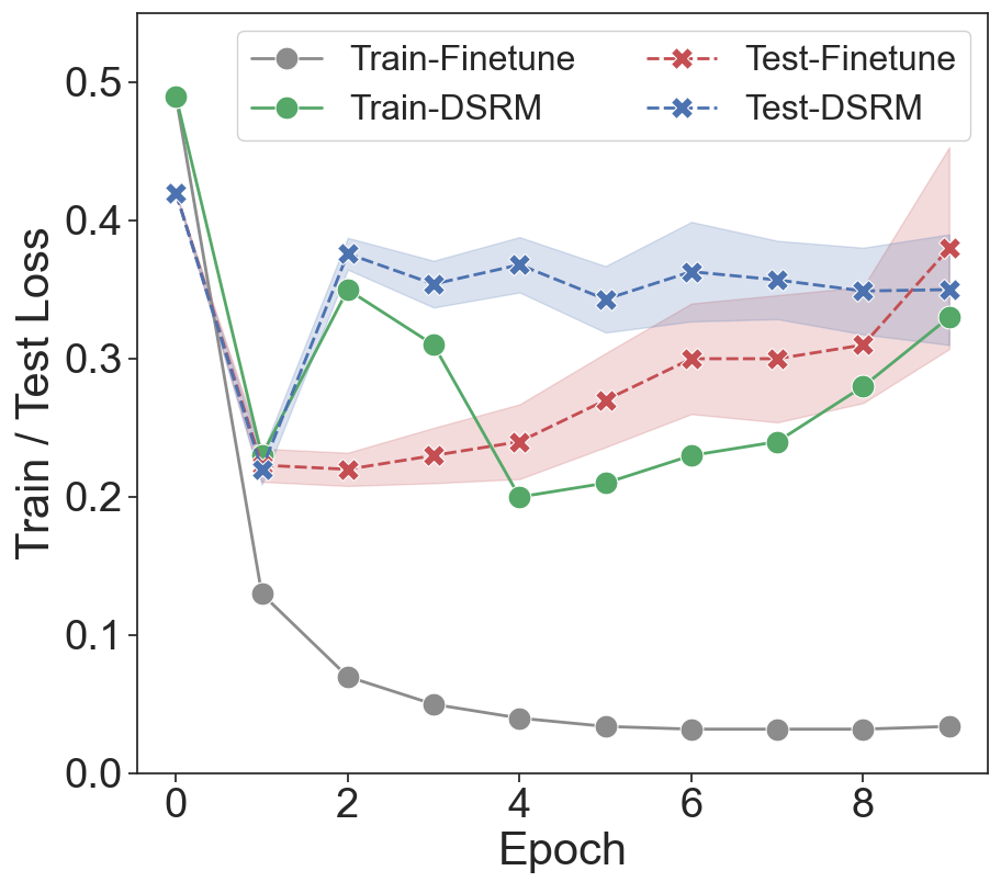
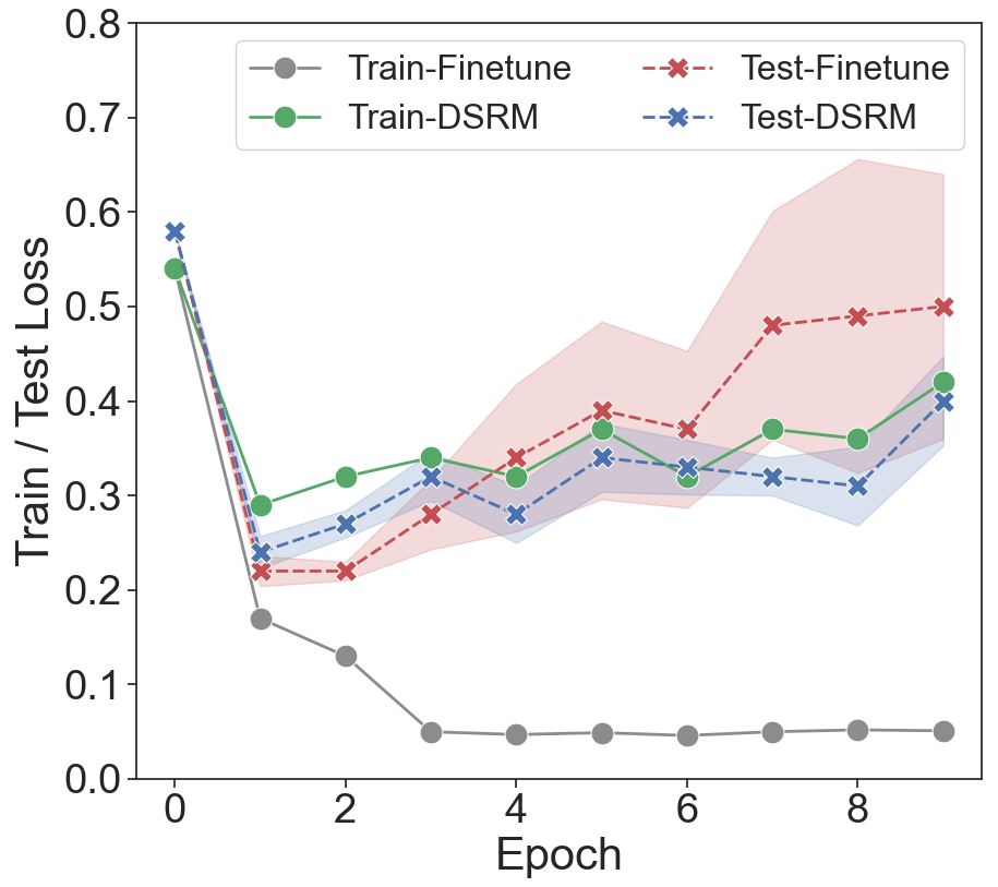
Figure 1: The train/test loss of DSRM and fine-tuning on the SST-2 (a) and IMDB (b) datasets. We report the mean loss on the train and test sets, and variance (marked with shadow) only on the test set. Our method maintains uniform loss distribution and better consistency between training and test data while the fine-tuning overfits quickly after one epoch.

5.2 Effect of Perturbation Intensity

DSRM has a single hyperparameter $\varepsilon$ to control the constraints on perturbation intensity. The extension in the perturbation range brings a better optimization on the defence objective, while the mismatch between the train and test set data distribution may impair the model performance. To further analyze the impact of DSRM on model accuracy and robustness, we conduct a sensitivity analysis of perturbation intensity $\varepsilon$. Figure 2 illustrates the variation curve of performance change for our method on three attack algorithms.

DSRM improves accuracy and Aua% when perturbations are moderated ($\leq 0.2$), similar to other adversarial training methods. When the perturbation becomes stronger, the model’s resistance to adversarial attacks improves notably and suffers a drop in clean accuracy. Such turning points occur earlier in our method, making it a trade-off between model accuracy and robustness. We argue that this phenomenon comes from the fact that the clean data distribution can be treated as a marginal distribution in the previous adversarial training, where the model can still fit the original samples.

Figure 2: Accuracy and Aua% of BERT trained by DSRM under different perturbations.

5.3 Time Consumption

In section 2, we analyze the positive correlation between training steps and model performance in adversarial training. Such trade-off in efficiency and effectiveness comes from the complex search process to find the optimal perturbation. DSRM circumvents this issue by providing upper-bound estimates with only clean data. To further reveal the strength of DSRM besides its robustness performance, we compare its GPU training time consumption with other adversarial training methods. As is demonstrated in Table 2, the time consumption of DSRM is superior to all the comparison methods. Only TAVAT Li and Qiu (2021) exhibits similar efficiency to ours (with about 30% time growth on SST-2 and IMDB). TAVAT neither contains a gradient ascent process on the embedding space, but they still require the construction of additional adversarial data. More experimental details are summarized in Appendix C.

Methods	SST-2	IMDB	AG NEWS
Finetune	227	371	816
DSRM	607	1013	2744
TAVAT	829	1439	2811
FreeLB	911	1558	3151
PGD	1142	1980	4236
FreeLB++	2278	3802	5348

Table 2: GPU time consumption (seconds) of training one epoch on the whole dataset.

5.4 Trade-offs in Standard Adversarial Training

In this section, we further discuss the trade-off between computational cost and performance in vanilla adversarial training. We empirically show that larger perturbation radii and steps enhance the effectiveness of textual adversarial training. Similar phenomena are previously found in image datasets by Zhang et al. (2019b) and Gowal et al. (2020). The experimental results for these two modifications are shown in Figure 3.

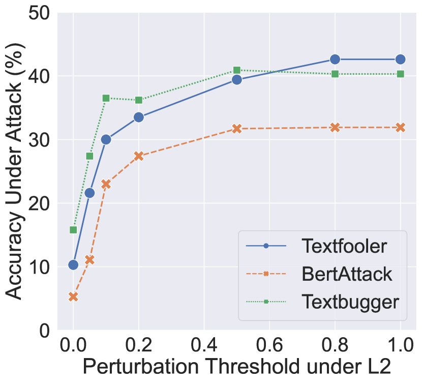
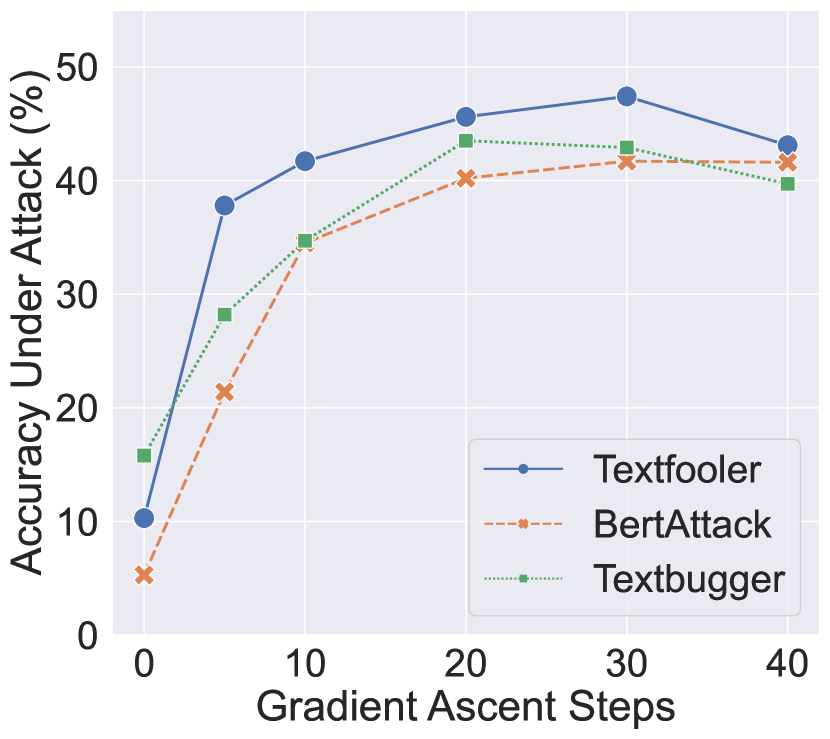
Figure 3: The impact of different values of the perturbation threshold (a) and ascent steps (b) on IMDB dataset. We show the accuracy score of the FreeLB Zhu et al. (2019) algorithm under three attack methods. Sub-figure (a) uses a 10-step gradient ascent with different constraints on the $l_{2}$ norm of perturbations. In sub-figure (b), each step introduces a perturbation of length 0.05.

In sub-figure (a), relaxing perturbation threshold remarkably increases the model robustness and only suffers a slight decrease when the threshold is larger than 0.6 for Textbugger. In subfigure (b), as the value of steps grows, the models’ accuracy under attack increases until they reach their peak points. Subsequently, they begin to decline as the number of steps increases consistently. Notably, the optimal results are 4-10% higher in (b) relative to (a), demonstrating that a larger number of steps is necessary to achieve optimal robustness.

We give a possible explanation for the above performance. We describe the standard adversarial training as exploring potential adversarial samples in the embedding space. When the step number is small, the adversarial sample space is correspondingly simple, causing the model to underestimate the adversarial risks. A broader search interval can prevent these defects and achieve outstanding robustness as the number of steps grows.

However, these best results occur late in the step growth process. As shown in (b), a defence model needs 30 steps (about ten times the time cost) for Textfooler, 20 for Textbugger, and 40 for BertAttack to achieve optimal performance. This drawback considerably reduces the efficiency and practicality of adversarial training.

6 Conclusion

In this paper, we delve into the training objective of adversarial training and verify that the robust optimization loss can be estimated by shifting the distribution of training samples. Based on this discovery, we propose DSRM as an effective and more computationally friendly algorithm to overcome the trade-off between efficiency and effectiveness in adversarial training. DSRM optimizes the upper bound of adversarial loss by perturbing the distribution of training samples, thus circumventing the complex gradient ascent process. DSRM achieves state-of-the-art performances on various NLP tasks against different textual adversarial attacks. This implies that adversarial samples, either generated by gradient ascent or data augmentation, are not necessary for improvement in adversarial robustness. We call for further exploration and understanding of the association between sample distribution shift and adversarial robustness.

7 Limitations

This section discusses the potential limitations of our work. This paper’s analysis of model effects mainly focuses on common benchmarks for adversarial defence, which may introduce confounding factors that affect the stability of our framework. Therefore, our model’s performance on more tasks, $e.g.$, the MRPC dataset for semantic matching tasks, is worth further exploring. In addition, the present work proposes to conduct adversarial training from the perspective of estimating the overall adversarial loss. We expect a more profound exploration of improving the accuracy and efficiency of such estimation. We are also aware of the necessity to study whether the properties of traditional methods, such as the robust overfitting problem, will also arise in DSRM-based adversarial training. We leave these problems to further work.

Appendix A Dataset Statistics

Dataset	Train/Test	Classes	#Words
SST-2	67k/1.8k	2	19
IMDB	25k/25k	2	268
AG NEWS	120k/7.6k	4	40
QNLI	105k/5.4k	2	37

Table 3: Statistics of datasets. In our experiments, we partition an additional 10 per cent of the training set as the validation set to calculate the DSRM of the model

Appendix B Experimental details

In our experiments, we calculate the sample weights by gradient ascending mean loss to a fixed threshold. The weight of each sample in the normal case is 1/n, where n is the size of a batch. We fine-tune the BERT-base model by the official default settings. For IMDB and AGNews, we use $10\%$ of the data in the training set as the validation set. The optimal hyperparameter values are specific for different tasks, but the following values work well in all experiments:

Batch Size and Max Length:

We use batch 16 and max length 128 for SST-2, QNLI, and AG NEWS datasets. For the IMDB dataset, we use batch 8 and max length 256 as its sentence are much longer than other datasets.

Perturbation Thresholds $\varepsilon$:

$\left[0.8,1,1.2,1.5\right]$. Weights are truncated when the adversarial loss is greater than the threshold.

Evaluation Settings:

For SST-2, we use the official test set, while for IMDB and AGNews, we use the first 1000 samples in the test set to evaluate model robustness. All three attacks are implemented using TextAttack with the default parameter settings.

Appendix C Training time measurement protocol

We measure the training time of each method on GPU and exclude the time for I/O. Each method is run three times and reports the average time. For a fair comparison, every model is trained on a single NVIDIA RTX 3090 GPU with the same batch size for each dataset (8 for IMDB and 32 for the other two datasets).

References

- Andriushchenko and Flammarion (2020) Maksym Andriushchenko and Nicolas Flammarion. 2020. Understanding and improving fast adversarial training. Advances in Neural Information Processing Systems, 33:16048–16059.
- Athalye et al. (2018) Anish Athalye, Nicholas Carlini, and David Wagner. 2018. Obfuscated gradients give a false sense of security: Circumventing defenses to adversarial examples. In International conference on machine learning, pages 274–283. PMLR.
- Cheng et al. (2020) Yong Cheng, Lu Jiang, Wolfgang Macherey, and Jacob Eisenstein. 2020. Advaug: Robust adversarial augmentation for neural machine translation. In Proceedings of the 58th Annual Meeting of the Association for Computational Linguistics, pages 5961–5970.
- Chiang and Lee (2022) Cheng-Han Chiang and Hung-yi Lee. 2022. How far are we from real synonym substitution attacks? arXiv preprint arXiv:2210.02844.
- Devlin et al. (2019) Jacob Devlin, Ming-Wei Chang, Kenton Lee, and Kristina Toutanova. 2019. Bert: Pre-training of deep bidirectional transformers for language understanding. In Proceedings of the 2019 Conference of the North American Chapter of the Association for Computational Linguistics: Human Language Technologies, Volume 1 (Long and Short Papers), pages 4171–4186.
- Goodfellow et al. (2015) Ian Goodfellow, Jonathon Shlens, and Christian Szegedy. 2015. Explaining and harnessing adversarial examples. In International Conference on Learning Representations.
- Gowal et al. (2020) Sven Gowal, Chongli Qin, Jonathan Uesato, Timothy Mann, and Pushmeet Kohli. 2020. Uncovering the limits of adversarial training against norm-bounded adversarial examples. arXiv preprint arXiv:2010.03593.
- Hauser et al. (2021) Jens Hauser, Zhao Meng, Damián Pascual, and Roger Wattenhofer. 2021. Bert is robust! a case against synonym-based adversarial examples in text classification. arXiv preprint arXiv:2109.07403.
- Ishida et al. (2020) Takashi Ishida, Ikko Yamane, Tomoya Sakai, Gang Niu, and Masashi Sugiyama. 2020. Do we need zero training loss after achieving zero training error? In International Conference on Machine Learning, pages 4604–4614. PMLR.
- Jin et al. (2020) Di Jin, Zhijing Jin, Joey Tianyi Zhou, and Peter Szolovits. 2020. Is bert really robust? a strong baseline for natural language attack on text classification and entailment. In Proceedings of the AAAI conference on artificial intelligence, volume 34, pages 8018–8025.
- Li et al. (2018) Jinfeng Li, Shouling Ji, Tianyu Du, Bo Li, and Ting Wang. 2018. Textbugger: Generating adversarial text against real-world applications. arXiv preprint arXiv:1812.05271.
- Li et al. (2020) Linyang Li, Ruotian Ma, Qipeng Guo, Xiangyang Xue, and Xipeng Qiu. 2020. Bert-attack: Adversarial attack against bert using bert. In Proceedings of the 2020 Conference on Empirical Methods in Natural Language Processing (EMNLP), pages 6193–6202.
- Li and Qiu (2021) Linyang Li and Xipeng Qiu. 2021. Token-aware virtual adversarial training in natural language understanding. In Proceedings of the AAAI Conference on Artificial Intelligence, volume 35, pages 8410–8418.
- Li et al. (2021) Zongyi Li, Jianhan Xu, Jiehang Zeng, Linyang Li, Xiaoqing Zheng, Qi Zhang, Kai-Wei Chang, and Cho-Jui Hsieh. 2021. Searching for an effective defender: Benchmarking defense against adversarial word substitution. In Proceedings of the 2021 Conference on Empirical Methods in Natural Language Processing, pages 3137–3147.
- Lin et al. (2021) Jieyu Lin, Jiajie Zou, and Nai Ding. 2021. Using adversarial attacks to reveal the statistical bias in machine reading comprehension models. In Proceedings of the 59th Annual Meeting of the Association for Computational Linguistics and the 11th International Joint Conference on Natural Language Processing (Volume 2: Short Papers), pages 333–342.
- Liu et al. (2022) Qin Liu, Rui Zheng, Bao Rong, Jingyi Liu, Zhihua Liu, Zhanzhan Cheng, Liang Qiao, Tao Gui, Qi Zhang, and Xuan-Jing Huang. 2022. Flooding-x: Improving bert’s resistance to adversarial attacks via loss-restricted fine-tuning. In Proceedings of the 60th Annual Meeting of the Association for Computational Linguistics (Volume 1: Long Papers), pages 5634–5644.
- Maas et al. (2011) Andrew Maas, Raymond E Daly, Peter T Pham, Dan Huang, Andrew Y Ng, and Christopher Potts. 2011. Learning word vectors for sentiment analysis. In Proceedings of the 49th annual meeting of the association for computational linguistics: Human language technologies, pages 142–150.
- Madry et al. (2017) Aleksander Madry, Aleksandar Makelov, Ludwig Schmidt, Dimitris Tsipras, and Adrian Vladu. 2017. Towards deep learning models resistant to adversarial attacks. arXiv preprint arXiv:1706.06083.
- Madry et al. (2018) Aleksander Madry, Aleksandar Makelov, Ludwig Schmidt, Dimitris Tsipras, and Adrian Vladu. 2018. Towards deep learning models resistant to adversarial attacks. In International Conference on Learning Representations.
- Morris et al. (2020) John Morris, Eli Lifland, Jin Yong Yoo, Jake Grigsby, Di Jin, and Yanjun Qi. 2020. Textattack: A framework for adversarial attacks, data augmentation, and adversarial training in nlp. In Proceedings of the 2020 Conference on Empirical Methods in Natural Language Processing: System Demonstrations, pages 119–126.
- Peyré et al. (2019) Gabriel Peyré, Marco Cuturi, et al. 2019. Computational optimal transport: With applications to data science. Foundations and Trends® in Machine Learning, 11(5-6):355–607.
- Rodriguez et al. (2021) Pedro Rodriguez, Joe Barrow, Alexander Miserlis Hoyle, John P Lalor, Robin Jia, and Jordan Boyd-Graber. 2021. Evaluation examples are not equally informative: How should that change nlp leaderboards? In Proceedings of the 59th Annual Meeting of the Association for Computational Linguistics and the 11th International Joint Conference on Natural Language Processing (Volume 1: Long Papers), pages 4486–4503.
- Shafahi et al. (2019) Ali Shafahi, Mahyar Najibi, Mohammad Amin Ghiasi, Zheng Xu, John Dickerson, Christoph Studer, Larry S Davis, Gavin Taylor, and Tom Goldstein. 2019. Adversarial training for free! Advances in Neural Information Processing Systems, 32.
- Shreya and Khapra (2022) Goyal Shreya and Mitesh M Khapra. 2022. A survey in adversarial defences and robustness in nlp. arXiv preprint arXiv:2203.06414.
- Si et al. (2021) Chenglei Si, Zhengyan Zhang, Fanchao Qi, Zhiyuan Liu, Yasheng Wang, Qun Liu, and Maosong Sun. 2021. Better robustness by more coverage: Adversarial and mixup data augmentation for robust finetuning. In Findings of the Association for Computational Linguistics: ACL-IJCNLP 2021, pages 1569–1576.
- Socher et al. (2013) Richard Socher, Alex Perelygin, Jean Wu, Jason Chuang, Christopher D Manning, Andrew Y Ng, and Christopher Potts. 2013. Recursive deep models for semantic compositionality over a sentiment treebank. In Proceedings of the 2013 conference on empirical methods in natural language processing, pages 1631–1642.
- Uesato et al. (2018) Jonathan Uesato, Brendan O’donoghue, Pushmeet Kohli, and Aaron Oord. 2018. Adversarial risk and the dangers of evaluating against weak attacks. In International Conference on Machine Learning, pages 5025–5034. PMLR.
- Wang et al. (2018) Alex Wang, Amanpreet Singh, Julian Michael, Felix Hill, Omer Levy, and Samuel R Bowman. 2018. Glue: A multi-task benchmark and analysis platform for natural language understanding. In International Conference on Learning Representations.
- Wang et al. (2020) Boxin Wang, Shuohang Wang, Yu Cheng, Zhe Gan, Ruoxi Jia, Bo Li, and Jingjing Liu. 2020. Infobert: Improving robustness of language models from an information theoretic perspective. In International Conference on Learning Representations.
- Wang et al. (2022) Jiayi Wang, Rongzhou Bao, Zhuosheng Zhang, and Hai Zhao. 2022. Distinguishing non-natural from natural adversarial samples for more robust pre-trained language model. In Findings of the Association for Computational Linguistics: ACL 2022, pages 905–915.
- Wang et al. (2021) Yisen Wang, Xingjun Ma, James Bailey, Jinfeng Yi, Bowen Zhou, and Quanquan Gu. 2021. On the convergence and robustness of adversarial training. arXiv preprint arXiv:2112.08304.
- Werpachowski et al. (2019) Roman Werpachowski, András György, and Csaba Szepesvári. 2019. Detecting overfitting via adversarial examples. Advances in Neural Information Processing Systems, 32.
- Wong et al. (2019) Eric Wong, Leslie Rice, and J Zico Kolter. 2019. Fast is better than free: Revisiting adversarial training. In International Conference on Learning Representations.
- Xi et al. (2022) Zhiheng Xi, Rui Zheng, Tao Gui, Qi Zhang, and Xuanjing Huang. 2022. Efficient adversarial training with robust early-bird tickets. arXiv preprint arXiv:2211.07263.
- Zeng et al. (2021) Guoyang Zeng, Fanchao Qi, Qianrui Zhou, Tingji Zhang, Zixian Ma, Bairu Hou, Yuan Zang, Zhiyuan Liu, and Maosong Sun. 2021. Openattack: An open-source textual adversarial attack toolkit. In Proceedings of the 59th Annual Meeting of the Association for Computational Linguistics and the 11th International Joint Conference on Natural Language Processing: System Demonstrations, pages 363–371.
- Zhang et al. (2019a) Dinghuai Zhang, Tianyuan Zhang, Yiping Lu, Zhanxing Zhu, and Bin Dong. 2019a. You only propagate once: Accelerating adversarial training via maximal principle. Advances in Neural Information Processing Systems, 32.
- Zhang et al. (2019b) Hongyang Zhang, Yaodong Yu, Jiantao Jiao, Eric Xing, Laurent El Ghaoui, and Michael Jordan. 2019b. Theoretically principled trade-off between robustness and accuracy. In International conference on machine learning, pages 7472–7482. PMLR.
- Zhang et al. (2015) Xiang Zhang, Junbo Zhao, and Yann LeCun. 2015. Character-level convolutional networks for text classification. Advances in neural information processing systems, 28.
- Zhou et al. (2021) Yi Zhou, Xiaoqing Zheng, Cho-Jui Hsieh, Kai-Wei Chang, and Xuan-Jing Huang. 2021. Defense against synonym substitution-based adversarial attacks via dirichlet neighborhood ensemble. In Proceedings of the 59th Annual Meeting of the Association for Computational Linguistics and the 11th International Joint Conference on Natural Language Processing (Volume 1: Long Papers), pages 5482–5492.
- Zhu et al. (2022) Bin Zhu, Zhaoquan Gu, Le Wang, Jinyin Chen, and Qi Xuan. 2022. Improving robustness of language models from a geometry-aware perspective. In Findings of the Association for Computational Linguistics: ACL 2022, pages 3115–3125.
- Zhu et al. (2019) Chen Zhu, Yu Cheng, Zhe Gan, Siqi Sun, Tom Goldstein, and Jingjing Liu. 2019. Freelb: Enhanced adversarial training for natural language understanding. In International Conference on Learning Representations.