Input-sensitive dense-sparse primitive compositions for GNN acceleration

Abstract.

Graph neural networks (GNN) have become an important class of neural network models that have gained popularity in domains such as social and financial network analysis. Different phases of GNN computations can be modeled using both dense and sparse matrix operations. There have been many frameworks and optimization techniques proposed in the literature to accelerate GNNs. However, getting consistently high performance across many input graphs with different sparsity patterns and GNN embedding sizes has remained difficult.

In this paper, we propose different algebraic reassociations of GNN computations that lead to novel dense and sparse matrix primitive selections and compositions. We show that the profitability of these compositions depends on the input graph, embedding size, and the target hardware. We developed SENSEi, a system that uses a data-driven adaptive strategy to select the best composition given the input graph and GNN embedding sizes. Our evaluations on a wide range of graphs and embedding sizes show that SENSEi achieves geomean speedups of $1.105\times$ (up to $2.959\times$) and $1.187\times$ (up to $1.99\times$) on graph convolutional networks and geomean speedups of $2.307\times$ (up to $35.866\times$) and $1.44\times$ (up to $5.69\times$) on graph attention networks on CPUs and GPUs respectively over the widely used Deep Graph Library. Further, we show that the compositions yield notable synergistic performance benefits on top of other established sparse optimizations such as sparse matrix tiling by evaluating against a well-tuned baseline.

1. Introduction

Graph Neural Networks (GNN) have gained considerable adoption across a wide range of application domains including social media marketing (nips2018:zhang:gnn-link-predcition, ), financial fraud detection (baba-fraud1, ; baba-fraud2, ), drug discovery (iclr2019:jin:drug-discovery, ; acs2019:torng:gcn-drug-interaction, ), and systems optimization (tpu-costmodel, ). However, training GNNs is expensive and usually spans multiple hours if not days. As a result, there have been many efforts including software frameworks such as DGL (iclr2019:wang:dgl, ), PyG (iclr2019:fey:pyg, ), and NeuGraph (atc2019:ma:neugraph, ), compilers such as Graphiler (graphiler, ) and many systems optimization techniques (mlsys2020:jia:roc, ; dorylus, ; zhang2021understanding, ; bridging-gap, ) that aim at accelerating GNN computations.

Usually, these systems model GNN computations as individual phases consisting of sparse or dense matrix operations. In a typical GNN layer, each node collects its neighbor node states (embeddings) and aggregates them. Next, each node updates its own state using these aggregated embeddings. The first computation is modeled as a set of sparse matrix operations and the latter is a dense matrix multiplication. Apart from these phases, different GNNs perform other required computations such as normalization and edge weight (attention score) calculations that are also modeled as either sparse or dense matrix operations. The aforementioned frameworks, compilers and optimization techniques mainly optimize these computations as individual phases and do not get consistent performance across graphs with different sparsity patterns and GNN embedding sizes.

Comparatively, in this work we specifically investigate different algebraic reassociations in GNN computations. These associations lead to interesting sparse and dense matrix primitive selections and compositions that may be profitable depending on the input graph structure and GNN embedding sizes. We introduce such input-sensitive compositions to GNN computations and propose an adaptive machine learning based strategy to select the most profitable compositions depending on the input graph and embedding sizes.

There has been recent work that performs dynamic optimizations specialized to a given input in GNNs. GNNAdvisor  (ding-gnnadvisor, ) considers the input graph for making the decision to perform reordering and selecting the optimum set of parameters for the computations that it performs on GPUs. (qiu:xgboost_format_selection_GNN, ) uses machine learning to select the best data representation for the sparse computation in GNNs. Meanwhile, (yan:feat_op_GNN_selection, ) uses the input and output embedding sizes of GNN layers to decide between sparse and dense primitive ordering. However, all of these techniques limit their adaptive decisions to one aspect of input sensitivity: whether it be the input graph or the embedding size, and miss the type of dense-sparse primitive compositions explored in this paper whose profitability depends on the combination of the input graph, GNN embedding size as well as the underlying hardware.

Our techniques are motivated by a key observation. Depending on the graph sparsity pattern and the embedding sizes of GNN layers, the bottleneck of the GNN computation can shift between the sparse matrix and the dense matrix operations. Table 1 shows the breakdown of runtimes for the sparse matrix (SpMM) and dense matrix (GEMM) operations as the input graph and embedding sizes change on graph convolution networks (GCNpaper, ), which is a popular GNN architecture. Note that in this scenario we consider the same input and output embedding sizes for a GNN layer. For much denser graphs (e.g. Reddit), sparse operations dominate the runtime, and for much sparser graphs (e.g. asia_osm), dense computations dominate. Also, as the embedding size increases the bottleneck can shift from sparse to dense (e.g. com-Liv). Therefore, it may be beneficial to use different algebraic reassociations that lead to different compositions of dense-sparse primitives for certain GNN computations depending on the input.

We leverage this observation to present novel input-sensitive dense-sparse primitive compositions targeted at two popular GNN models: graph convolution networks (GCN) (GCNpaper, ) and graph attention networks (GAT) (iclr2018:velic:gat, ). In the GCN case, we propose to either perform normalization as a standalone phase (precompute) or as a part of the aggregate and update computations (dynamic). In the GAT case, we propose to either reuse updated embeddings from the attention calculation phase (reuse) or recompute them dynamically (recompute). The computation of each method requires a different composition of dense-sparse primitives and as such the profitability of each depends on how fast each primitive executes. As shown in Table 2 and 3, the composition selection has a direct impact on the runtime performance of these GNNs. Also note that these compositions are not limited to GCN and GAT and can be generalized to other models. Furthermore, techniques such as sampling are orthogonal to the compositions presented in this work and can work alongside them to optimize GNN performance. We bring this topic into discussion in section 7.

To this end, we developed SENSEi, a system to decide on which composition to use under each scenario depending on the input graph and GNN embedding sizes. Our evaluations (Section 6.6) show that selecting the best composition in every case just based on a single hard-coded metric is sub-optimal. Therefore, SENSEi uses an adaptive machine learning model that is parameterized based on the input graph features and GNN embedding size to decide which composition to use to achieve runtime speedups. We train the model using a dataset of apriori collected executions and show that SENSEi is able to predict with high accuracy the best dense-sparse primitive composition to use.

We extended the widely adopted GNN framework, Deep Graph Library (DGL) (iclr2019:wang:dgl, ) to allow for the different primitive composition choices. We use SENSEi to select the best composition choice for both GCN and GAT under inference and training running on both CPUs and GPUs. Our evaluation reveals that SENSEi is effective in all scenarios. For example, SENSEi achieves up to $1.99\times$ over DGL in GCN inference and up to $5.69\times$ over DGL in GAT inference on GPUs with very little overhead over a wide variety of input graphs with different sparsity patterns. Section 6.3 gives detailed results for each setting.

Further, we investigated the behavior of the compositions in the presence of other established optimizations such as sparse matrix tiling. Since DGL does not support optimizations such as tiling, we implemented the compositions on top of an optimized CPU implementation that supports advanced hardware-aware optimizations. We then investigated the benefits of selecting the most profitable primitive compositions. Our results show clear synergistic performance improvements even when other optimizations are applied. Overall, SENSEi shows that selecting the best dense-sparse primitive composition adaptively based on the input leads to sizable performance improvements in GNN computations across different hardware platforms and different software implementations.

Table 1. SpMM and GEMM execution times (s) for a GCN layer on different graphs and embedding sizes (40 iterations) Bottlenecks are bolded.

Graph	Op	Embedding size
		32	128	512	2048
Reddit	SpMM	0.816	3.581	28.548	170.262
	GEMM	0.019	0.114	0.985	10.660
com-Liv	SpMM	1.871	6.795	29.222	113.302
	GEMM	0.526	2.277	14.689	177.299
aisa_osm	SpMM	1.249	4.107	15.912	63.667
	GEMM	1.515	6.321	43.818	528.987

In this paper, we make the following specific contributions.

• We introduce algebraic reassociations that lead to novel input-sensitive primitive compositions involving both sparse and dense matrix primitives for popular GNN models GCN and GAT.

• We present SENSEi, a system that uses a machine learning based strategy to select the best composition given an input graph and the GNN embedding sizes.

• We evaluate SENSEi on a wide variety of graphs with different sparsity patterns and on a wide range of embedding sizes and show that it predicts the best primitive composition to use on both CPUs and GPUs with high accuracy.

• We implement the compositions on top of DGL and show that SENSEi’s decisions lead to $1.105\times$ (up to $2.959\times$) and $1.187\times$ (up to $1.99\times$) geomean speedup for GCN, and $2.307\times$ (up to $35.866\times$) and $1.44\times$ (up to $5.69\times$) geomean speedup for GAT for CPU and GPU respectively. We further implement the compositions in separate optimized baselines to investigate the synergies with other optimizations such as sparse tiling. Our results show that SENSEi is able to achieve up to $1.218\times$ speedup for GCN, and up to $2.94\times$ speedup for GAT on CPU.

2. Background

We first briefly introduce the sparse matrix primitives and the GNN computations of GCN and GAT to facilitate the discussion of different dense-sparse primitive compositions in Section 3.

2.1. Sparse Matrix Primitives

Computations used in GNN models can be modeled using both dense and sparse matrix computations (iclr2019:wang:dgl, ). Dense matrix computations mainly consist of the general matrix multiplication (GEMM) that is widely found in other neural network models. The sparse computations mainly consist of two primitives. These are the generalized forms of sparse matrix dense matrix multiplication (SpMM) and sampled dense dense matrix multiplication (SDDMM). The standard SpMM and SDDMM use $+$ and $\times$ as the addition and multiplication operators, whereas in the generalized form, these can come from any semi-ring (davis:graphblas, ). We use $\oplus$ and $\otimes$ to signify these generalized addition and multiplication operators. Also, we use the notation $a_{i,j}$ to refer to the value at row $i$ and column $j$ of a given matrix $A$.

Generalized sparse matrix dense matrix multiplication (g-SpMM)

g-SpMM takes one input sparse matrix $A$ and multiplies ($\otimes$) that by an input dense matrix $B$ to produce a dense output matrix $C$. Equation 1 shows how $c_{i,k}$ of $C$ is computed.

(1) $$c_{i,k}=\sum_{\oplus,j}a_{i,j}\otimes b_{j,k}$$

The computation mirrors that of GEMM. However, note that when $a_{i,j}$ is zero, there is no contribution to the output. Since $A$ is sparse, the majority of its entries are zeroes. Thus, SpMM leverages the sparsity of input matrix $A$ to skip any multiplications without contributions compared to GEMM.

Generalized sampled dense dense matrix multiplication (g-SDDMM)

g-SDDMM performs a computation between two dense input matrices $B$ and $C$ controlled by the non-zero (nnz) values of a sparse matrix $A$. This results in an output sparse matrix $D$ with a sparsity pattern matching that of $A$. Equation 2 shows how each element $d_{i,j}$ of $D$ is computed.

(2) $$d_{i,j}=\begin{dcases}a_{i,j}\otimes\sum_{\oplus,k}b_{i,k}\otimes c_{j,k},&\text{if }a_{i,j}\text{ not }0\\ 0,&\text{otherwise}\end{dcases}$$

In g-SDDMM, a multiply ($\otimes$) operation is performed between $b_{i,k}$ and $c_{j,k}$, for all $k$ if and only if the value of $a_{i,j}$ is non-zero. The partial products are then summed up ($\oplus$) and multiplied with $a_{i,j}$ to form the $d_{i,j}$ scalar value. This, in a sense, is again similar to GEMM with two dense input matrices. However, in g-SDDMM, the input sparse matrix is used as a mask to selectively compute values instead of performing the entire dense matrix multiplication.

2.2. Graph Neural Networks

Graph neural networks consist of two main stages: aggregation and update. Each node or edge has an embedding modeled as a hidden state vector. During the aggregation stage, these embeddings are passed among neighbors to form an aggregated message. In the update stage, these messages are then transformed into updated embeddings as the GNN layer’s output. Usually, these computations are modeled as a collection of sparse and dense primitive operations (iclr2019:wang:dgl, ). Node-based aggregations are modeled as g-SpMM operations, while edge-based aggregations are modeled as g-SDDMM operations. The update is modeled as a GEMM computation.

Apart from these stages, there are other required computations such as normalization that open up more opportunities to consider different algebraic reassociations leading to different dense-sparse primitive compositions. In this work, we focus on two popular GNN models – GCN and GAT – to showcase such compositions that can lead to performance benefits. Note that, these compositions are not limited to GCN or GAT and can be generalized to other GNN models with normalization and edge-weight calculations. We now present both GCN and GAT computations in matrix form.

Graph Convolutional Networks

The inference computation of a Graph Convolutional Netowk (GCN) (GCNpaper, ) for an undirected graph on the $(l)^{th}$ layer is presented by Equation 3.

(3) $$H^{(l)}=\sigma(\tilde{D}^{-\frac{1}{2}}\cdot\tilde{A}\cdot\tilde{D}^{-\frac{1}{2}}\cdot H^{(l-1)}\cdot W^{(l)})$$

Here, $\tilde{A}$ is the adjacency matrix of the graph augmented with self-edges. $\tilde{A}$ is usually represented as a sparse matrix and its sparsity pattern depends on the topology of the graph. $\tilde{D}$ is the degree matrix of this augmented graph and is represented as a diagonal matrix.

$H^{(l)}$, $W^{(l)}$ are the node embeddings and weights for the $l^{th}$ layer in the GNN respectively and both are represented as dense matrices. After performing the necessary computations between the aforementioned matrices, the non-linearity function $\sigma$ is applied to the result.

Graph Attention Network

The primary computation of a single-headed Graph Attention Network (GAT) (iclr2018:velic:gat, ) model can be represented as follows.

(4) $$\alpha^{(l)}=AttenCalc(\tilde{A},H^{(l-1)}\cdot W^{(l)},{W_{A}}^{(l)})$$

(5) $$H^{(l)}=\sigma({\alpha}^{(l)}\cdot H^{(l-1)}\cdot W^{(l)})$$

A graph edge processing function (AttenCalc) is used to produce the attention scores in GAT. For this, the updated input embeddings of the nodes ($H^{(l-1)}\cdot W^{(l)}$), and the weights used for attention ${W_{A}}^{(l)}$ are necessary. In addition, we also pass along $\tilde{A}$ to avoid unnecessary computations by not computing attention scores between nodes without connecting edges, similar to the process mentioned in the original GAT (iclr2018:velic:gat, ) paper. The result is a sparse matrix $\alpha$ containing the necessary attention scores and having the same non-zero distribution as the adjacency matrix $\tilde{A}$. This result is then used for the aggregation and update stages, as shown by Equation 5. An eye trained for optimization would see that $H^{(l-1)}\cdot W^{(l)}$ is calculated multiple times (in both Equations 4 and 5). Thus, it would be obvious to reuse the computed result. However, we show in Section 3.2 that this is not always the case and that it depends on the input. For this work in particular, we focus on single-headed GAT, but we believe that the same conclusion can be extended to multi-headed GAT.

3. GNN dense-sparse primitive compositions

As shown through the examples in Table 1, the most dominant computation in a GNN can be either sparse or dense primitives. This is determined by the embedding sizes of the GNN model as well as the input graph. Through algebraic reassociations, we were able to identify two input-sensitive primitive compositions for both GCN and GAT that may be profitable depending on which primitives are cheaper. In the rest of the section, we elaborate on these compositions and give evidence of their input sensitivity. We use these observations to design an input-sensitive learned decision system SENSEi as detailed in Section 4 that achieves considerable performance benefits in both GCN and GAT computations.

3.1. GCN: Normalization

Normalization in GCN for an un-directed graph occurs through $\tilde{D}^{-\frac{1}{2}}\cdot\tilde{A}\cdot\tilde{D}^{-\frac{1}{2}}$. Incorporating the aforementioned calculation into the GCN computation shown by equation 3, is possible through two different methods comprising of different dense-sparse primitives. This variation is possible due to the associative property of the computations involved.

(6) $$\begin{split}\tilde{N}&=\underbrace{(\tilde{D}^{-\frac{1}{2}}\cdot\tilde{A}\cdot\tilde{D}^{-\frac{1}{2}})}_{\text{SDDMM}}\phantom{X}H^{(l)}=\sigma(\underbrace{\tilde{N}\cdot H^{(l-1)}\cdot W^{(l)}}_{\text{SpMM, GEMM}})\end{split}$$

Precomputation based primitive composition

We first precompute the normalized adjacency matrix $\tilde{N}$ as shown in Equation 6 independently of any specific layer in the GCN, and then reuse the result during the aggregate stage of the model. The initial precomputation is possible through a g-SDDMM operation with the semirings used being the same as regular SDDMM. To elaborate, due to $\tilde{D}^{-\frac{1}{2}}$ being a diagonal matrix, $\tilde{D}^{-\frac{1}{2}}\cdot\tilde{A}$ is essentially an in-place multiplication of each value in row $i$ in $\tilde{A}$ with the $i^{th}$ element in the diagonal of $\tilde{D}^{-\frac{1}{2}}$. Similarly, $\tilde{A}\cdot\tilde{D}^{-\frac{1}{2}}$ is essentially an in-place multiplication of each value in column $j$ in $\tilde{A}$ with the $j^{th}$ element in the diagonal of $\tilde{D}^{-\frac{1}{2}}$. Thus, the value of an element in $\tilde{N}$ can be represented as in Equation 7.

(7) $$\tilde{n}_{i,j}=\tilde{a}_{i,j}\times(\tilde{d}^{-\frac{1}{2}}_{i}\times\tilde{d}^{-\frac{1}{2}}_{j})$$

This computation in Equation 7 matches the one for g-SDDMM as presented in Equation 2 once appropriate semirings are assigned and assuming that $k=1$. The normalization computation can thus be achieved through g-SDDMM, with the dense vector $\tilde{D}^{-\frac{1}{2}}$ serving as the two dense inputs and $\tilde{A}$ as the sparse input. We then use the precomputed result $\tilde{N}$ during the g-SpMM used for aggregation to incorporate the normalization into the final output.

Dynamic normalization based primitive composition

Here, we perform normalization through two GEMM operations without needing to rely on a sparse computation as shown by Equation 8. We initially perform a GEMM operation to incorporate the normalization factor ($\tilde{D}^{-\frac{1}{2}}H^{(l)})$ into the node embeddings. Then following the aggregation and update stages, another GEMM operation is performed to incorporate the second normalization factor ($\tilde{D}^{-\frac{1}{2}}H^{(l)})$ into the node embeddings. Through these two GEMM primitives, it is possible to perform the normalization without the need for a sparse primitive. However, unlike the precomputation method, this normalization calculation must be repeated during each layer and iteration.

(8) $$H^{(l)}=\sigma\underbrace{(\tilde{D}^{-\frac{1}{2}}\cdot\underbrace{(\tilde{A}\cdot\underbrace{(\tilde{D}^{-\frac{1}{2}}\cdot H^{(l-1)})}_{\text{GEMM}}\cdot W^{(l)})}_{\text{SpMM, GEMM}})}_{\text{GEMM}}$$

Decision points and insights

The two forms of primitive compositions result in different execution times based on the input graph and on the model’s input and output embedding sizes. A snippet of the observations is presented in Table 2.

Table 2. Speedup of precompute primitive composition over dynamic primitive composition for different graphs and embedding sizes

Graph	Input size, output size
	32,32	32,1024	1024,1024
mycielskian17	0.133	0.153	0.068
packing..b050	0.864	1.619	0.766
asia_osm	1.802	2.689	1.253

Considering unweighted graphs, in the dynamic primitive composition, one can make use of the fact that all nnz values of the original matrix $\tilde{A}$ are equal to one. Due to this fact, during aggregation, it is possible to completely avoid reading the value of an edge as shown in Equation 9. This, naturally, reduces the memory footprint of the sparse operation. Thus, although the dynamic primitive composition requires two additional GEMM computations, the GEMM overhead might be compensated by the reduced load in one of the major sparse operations. Using this point, we can explain the observation in Table 2: denser graphs (mycielskian17) achieve higher performance with the dynamic primitive composition as their major bottleneck is the sparse computation (recall the GEMM-SpMM runtime comparison of Table 1). However, the overhead of adding additional GEMM computations outweighs any benefit for the sparse primitives when the sparse asia_osm graph is considered.

(9) $$h^{(l)}_{i,k}=\sum_{\oplus,j}1\otimes h^{(l-1)}_{j,k}=\sum_{\oplus,j}h^{(l-1)}_{j,k}$$

There is an interesting observation when the input embedding size ($k1$), is different from the output embedding size ($k2$) of a GNN layer. We use the technique suggested in (yan:feat_op_GNN_selection, ) to select the order of aggregation and update phases. This order is selected so that the smaller embedding size is used for aggregation. As a result, in both our precompute and dynamic primitive compositions, the g-SpMM operation is performed on an embedding size which is $min(k1,k2)$. However, in the dynamic composition, the additional GEMM computations operate on embedding sizes of both $k1$ and $k2$. Thus, if there is a difference in embedding size ($k1<k2,k1>k2$), the dynamic composition will need to perform a GEMM on an embedding size larger than the one used for the SpMM operation. This may be more costly than the time saved by aggregation. Because of this, when different input and output embedding sizes are used, the precompute-based primitive composition becomes more profitable in comparison to a scenario with equal embedding sizes ($k1=k2$). This is illustrated in Table 2 where for packing-500x100x100-b050, the optimal primitive composition changes from dynamic to precompute when the embedding sizes differ.

3.2. GAT: Recomputation vs. Reuse

In GAT models we found two different primitive compositions that are related to the reuse of updated embeddings ($H\cdot W$). Assume a GAT layer with input embedding size $k1$ and output embedding size $k2$. During the attention score calculation, we compute the multiplication of the input embedding with the relevant weights ($H\cdot W$) to produce the updated embeddings as shown by equation 10. This attention calculation step is common for both primitive compositions. The difference lies in the decision taken during aggregation.

(10) $$\alpha^{(l)}_{n\times n}=AttenCalc(\tilde{A}_{n\times n},\underbrace{H^{(l-1)}_{n\times k1}\cdot W^{(l)}_{k1\times k2}}_{(H\cdot W)^{(l)}_{n\times k2}},{{W}^{(l)}_{A}}_{k2\times 1})$$

(11) $$H^{(l)}=\overbrace{{\alpha}^{(l)}_{n\times n}\cdot\underbrace{(H\cdot W)^{(l)}_{n\times k2}}_{\text{reuse}}}^{\text{SpMM\_k2}}$$

(12) $$H^{(l)}=\overbrace{\mathrlap{\overbrace{\phantom{(\alpha^{(l)}_{n\times n}\cdot H^{(l-1)}_{n\times k1})}}^{\text{SpMM\_k1}}}{(\alpha}^{(l)}_{n\times n}\cdot\underbrace{H^{(l-1)}_{n\times k1})\cdot W^{(l)}_{k1\times k2}}_{\text{recomputation}}}^{\text{GEMM}}$$

Reuse based primitive composition

Shown by Equation 11, this primitive composition focuses on reducing redundant computation. During aggregation, it simply reuses the updated embeddings that have already been computed in the attention calculation stage.

Recomputation based primitive composition

Shown by Equation 12, this primitive composition forgoes the reuse of the updated embeddings and uses the original embeddings for aggregation. However, this requires an additional update to the embeddings through a GEMM computation.

Decision points and insights

Which method is more profitable depends on both $k1,k2$ and the input graph. When $k1>k2$ or $k1=k2$ it is always beneficial to reuse the updated embeddings from the attention calculation stage. On the other hand, when $k1<k2$, recomputation may be more beneficial. This is because the SpMM operation will be performed on the smaller embedding size ($k1$). However, recomputation will only make sense if the time it takes for the additional GEMM is less than the time saved by performing the SpMM operation at embedding size $k1$. This is often the case with graphs with a larger number of edges compared to nodes (comparatively denser). Thus, when the difference in embedding size between $k1,k2$ grows larger, recomputation would become more beneficial. However, if the relative difference between the embeddings stays the same but with both $k1,k2$ increasing, then reuse may become more beneficial.

Table 3. Timing breakdowns for GAT recomputation vs reuse based primitive compositions; $k_{1}$ and $k_{2}$ are input and output embedding sizes

Graph	k1	k2	SpMMk1(s)	SpMMk2(s)	GEMM(s)	Reuse(s)	Recomp(s)	Recomp. better?
mycielskian17	32	256	0.42	3.14	0.003	3.37	0.60	$\surd$
	32	2048	0.42	23.88	0.015	24.03	0.65	$\surd$
	1024	2048	12.02	23.88	0.11	24.06	12.19	$\surd$
asia_osm	32	256	0.06	0.4	0.13	1.54	1.25	$\surd$
	32	2048	0.06	2.95	1.19	9.16	7.45	$\surd$
	1024	2048	1.45	2.95	7.77	15.44	22.67	$\times$

Table 3 presents the breakdown of the different computations involved under both methods for graphs with different sparsity patterns and conforms with the hypothesis stated prior. mycielskian17 (comparatively denser) graph sees a considerable benefit with recomputation compared to reuse, as its SpMM operation is more expensive than the GEMM. For asia_osm (comparatively sparser), even though it initially showed benefits from recomputation, as the embedding size increases, reuse becomes better.

4. SENSEi System

We present SENSEi: an input-sensitive decision-making system, that exploits the input-sensitivity of primitive compositions derived from different algebraic reassociations to achieve performance benefits in GNN computations.

4.1. Overview

The architecture of the proposed system, SENSEi, is shown in Figure 1(a). At a high level, SENSEi consists of two stages, the offline learning stage (Figure 1(b)) and the online execution stage (Figure 1(c)). In the learning stage, we train a ranking model based on profiling data gathered on many GNN execution configurations for the different primitive compositions suggested in Section 3. Then in the execution stage, given the characteristics of the input graph, GNN model architecture, as well as primitive compositions, the leaned model chooses the best among the compositions presented. This primitive composition is then used by the GNN execution system.

(a) SENSEi decision maker. Given a graph, model architecture, optimization configurations, and primitive compositions selects the best composition

(b) Stage 1 - Learning (Offline). Train SENSEi using profiling data of various graphs, model architectures, and primitive compositions

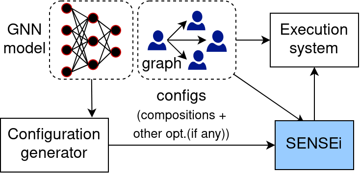
(c) Stage 2 - Execution (Online). SENSEi selects the best composition and passes the decision to the execution system

Figure 1. Overview of the SENSEi system

4.2. Ranking model for composition selection

SENSEi uses a tree-based XGBoost ranking model (XGBoost, ), which we name the composition selector, that predicts the best composition for a given input graph, embedding sizes, setting of auxiliary optimizations (e.g. sparse matrix tiling), and the underlying hardware architecture.

4.2.1. Graph feature extractor

We handcraft a set of features from the input graph as listed under Table 4. We could have used a neural network such as a sparse convolutional network(Xipeng2018:SparseConvNet, ) to automatically extract features, but this would hinder the scalability of SENSEi. One of the goals of designing SENSEi was to facilitate large graphs such as ogbn-products (2M nodes and 126M non-zeros). However, NN-based automatic feature extractors do not scale or are too expensive to use in this setting (waco, ). As shown in Section 6.5, the overhead of the entire SENSEi system is very minimal. The graph feature extractor, given the input graph, computes the features in Table 4 and passes it along to the learned model to be used in either training or inference.

Table 4. Graph features used in SENSEi’s composition selector

Feature	explanation/source
$n\_rows$	Total number of rows, i.e. nodes
$n\_nnzs$	Total number of non-zeros
$nnz\_den$	Density of the graph ($n\_nnzs/{n\_rows}^{2}$)
$nnz\_mean$	Mean number of non-zeros per node ($n\_nnzs/n\_rows$)
$d\_min$	Minimum degree of any node
$d\_max$	The maximum degree of any node
$d\_dentr$	Degree distribution entropy (powerlaw-feats, )
$e\_dentr$	Edge distribution entropy (powerlaw-feats, )

4.2.2. Composition selector

We use an XGBoost (XGBoost, ) tree model as the learned composition selector. The selector expects the graph features, model architecture, auxiliary optimization configurations (if any), and primitive composition considered as input and provides a relative ordering of the profitability of each different choice. Since we consider two primitive compositions for each GNN model, the selector’s decision is binary. We create a separate selector for each GNN considered by SENSEi. This allows us to easily add specialized GNN compositions for each GNN model.

4.2.3. Profile Data Collection

We collected many profiling runs to train the composition selector. Using a predetermined set of graphs and embedding sizes, we obtain their runtimes offline for the different primitive compositions. The graphs and embedding sizes chosen for the profiling must be representative of the graphs and embedding sizes SENSEi would use to later make decisions on during execution.

4.3. Execution system

Once a decision is made by SENSEi, it is passed to the system that will execute it. We implemented the GNN primitive compositions mentioned in Section 3, and enable the composition selection as a parameterized option. In its current state SENSEi provides decisions for two execution systems. One is implemented on top of the popular GNN framework DGL (iclr2019:wang:dgl, ), and the other is a well-tuned implementation with traditional sparse optimizations.

DGL execution system (DGL)

We implemented the different primitive compositions using the node and edge primitive functions of DGL. We show the effect of SENSEi’s decisions in Section 6.3.

Optimized execution system (OPT)

We implemented a tuned baseline of the GNNs augmented with other sparse optimizations in CPU, to confirm that the primitive compositions that we present see benefits not only in DGL, but can also give synergistic benefits with other optimized kernels as well. We present an evaluation for this execution system in Section 6.4.

We considered two sparse optimizations found in literature for this execution system: sparse tiling and reordering. For tiling, we first partition the input sparse matrix into column segments and then perform tiling based on rows. Depending on the tiling factor, the execution can lead to either excessive slowdowns or considerable speedups ($3\times$) – whether the optimizations are beneficial or not is determined by the input graph. Similarly, the benefit of reordering is also input-sensitive. This depends on the nnz distribution of the input graph. This nnz distribution may already maximize data locality without reordering needed. Performing reordering in such cases presents the possibility that the resulting nnz distribution may be worse than the original, leading to sub-optimal performance during sparse computations.

Since these two optimizations are input-sensitive, we auto-tuned them to achieve an optimized baseline based on the input graph. We select the optimal configuration of sparse tile size and whether to perform reordering or not using a ranking model similar to the selector used by SENSEi. We select the top 20 suggested by the ranker and perform an empirical auto-tuning to identify the best one. We then feed this selection into SENSEi as the optimization configuration.

5. Implementation

In this section, we explain our training setup and how we implemented the feature extractor and optimized execution system.

5.1. Training

We collect the training data necessary for the model by profiling different optimization configurations on the machines listed below. We also use the same machines for evaluation.

• CPU - Intel Xeon Gold 6348: (L2 cache 1.28MB, LLC 86MB), RAM 1TB, No GPU

• GPU - A100 GPU: (8GB), Intel Xeon Platinum 8358, RAM 256GB

We use both machines to collect training data for the evaluation of the DGL execution system but focused on CPU for the optimized execution (OPT) system. We source the input graphs from the SuiteSparse matrix collection. Here, we choose all undirected graphs ranging from 10 million to 25 million non-zero values. Considering the DGL execution, we varied different input and output embedding sizes, and primitive compositions to obtain approximately 625 and 250 data points for each machine. For OPT, in addition to the parameters varied previously we also considered different tiling configurations and reordering. This led to approximately 38,000 and 19,000 data points collected for GCN and GAT respectively on CPU.

After obtaining all the necessary data, we train the XGBoost model using the $gpu\_hist$ tree method, $dart$ booster, $rank:pairwise$ objective. This choice is common for the models of both systems. For the DGL models we used $300$ estimators and $0.001$ learning rate, and for the OPT models, we used $410$ estimators and $0.05$ learning rate. In particular for the DGL models we combined the data for both machines to create a model that is common for all machines due to the low amount of data points. We differentiate each machine by passing additional parameters such as machine architecture type, LLC size, etc, to the model.

5.2. Feature extractor and optimized system

The graph feature extractor and OPT were implemented in C++. The profiling data were collected utilizing code generated by #ifdef macros in C++ to easily compose optimization choices. However, the executor itself was built in a parameterized manner to reduce the overhead of not only preprocessing but also repeated compilation. We used the BLAS GEMM function from MKL and a third-party library for reordering.

6. Evaluation

We evaluate SENSEi by comparing against the default dense-sparse primitive composition for GNN inference and training found in DGL. For this evaluation, we test across various graphs (1 million to 126 million non-zeros with different sparsity patterns) in both CPU and GPU platforms. We used multiple combinations of input and output embedding sizes to showcase different trends in the performance of different input-sensitive compositions. We present detailed setups used for evaluation, along with performance results and various analyses in the subsequent sections.

6.1. Research questions

We aim to answer the following research questions through the evaluations done.

1. Does SENSEi get performance benefits for GCN and GAT on a diverse set of input graphs and embedding sizes across multiple hardware platforms? We evaluate SENSEi on the DGL execution system to answer this question (Section 6.3).

2. Does SENSEi get synergistic benefits over some optimized baselines? We evaluate SENSEi on the OPT execution system to answer this question (Section 6.4).

3. What are the overheads of SENSEi? We compare the additional time needed for any information gathering as well as preprocessing (Section 6.5).

4. How good is the learned model of SENSEi and what features are important when making decisions? We evaluate the decisions made by the learned model and compare them against the ground truth speedups of the best primitive compositions made by an oracle (Section 6.6).

In Section 6.2, we describe the detailed experimental setup used to answer these questions.

6.2. Experimental Setup

We use the Pytorch (Pytorch, ) backend of DGL (iclr2019:wang:dgl, ) for our comparison studies. We evaluate SENSEi on the machines listed in Section 5.1. The graphs used for evaluations are shown in Table 5. We selected the graphs to encompass multiple variations of non-zero distributions as well as scale. The evaluation set contains graphs ranging from 1 million non-zeros up to over 126 million. Among the various graph types that are included are road graphs (asia_osm), banded diagonal graphs (packing..b050), and power law graphs(Reddit). We sourced these graphs from three main locations. These were SuiteSparse (SS) (SuiteSparse, ): which provided a plethora of graphs of varying characteristics, DGL and Open Graph Benchmark (OGB) (hu2020:ogb, ): which provided graphs commonly used in the GNN context. Similar to the training data gathered, the graphs collected for the evaluation were undirected. In contrast to the graphs used for training, those selected for the evaluation possessed non-zeros ranging from below the minimum and the maximum found in the training dataset. This allows us to evaluate the generalization capability of SENSEi’s learned selector.

Table 5. Graphs used for evaluation

Graph	Nodes	Edges	Source
Reddit	232,965	114,615,892	DGL
ogbn-products	2,449,029	126,167,053	OGB
coAuthorsCiteseer	227,320	1,855,588	SS
com-Amazon	334,863	2,186,607	SS
belgium_osm	1,441,295	4,541,235	SS
com-Youtube	1,134,890	5,975,248	SS
asia_osm	11,950,757	25,423,206	SS
packing-500x	2,145,852	34,976,486	SS
100x100-b050
com-LiveJournal	3,997,962	69,362,378	SS
mycielskian17	98,303	100,245,742	SS

We use a single layer GNN for evaluation, and Table 6 shows the combinations of input-output embedding sizes that we tested. An extension to a multi-layered GNN is straightforward by making decisions for each individual layer separately. Also, we only evaluate increasing embedding sizes for GAT as this is the scenario in which the primitive composition choice is non-trivial. We also consider all of the graphs as unweighted for the evaluations.

Table 6. Embedding sizes used for evaluation

GNN	Input	Output	Category
	embedding size ($k_{1}$)	embedding size ($k_{2}$)
GCN	32	32	$k_{1}=k_{2}$
	32	256	$k_{1}<k_{2}$
	1024	32	$k_{1}>k_{2}$
	1024	1024	$k_{1}=k_{2}$
	1024	2048	$k_{1}<k_{2}$
GAT	32	256	$k_{1}<k_{2}$
	32	2048	$k_{1}<k_{2}$
	1024	2048	$k_{1}<k_{2}$

6.3. Performance Comparison with DGL

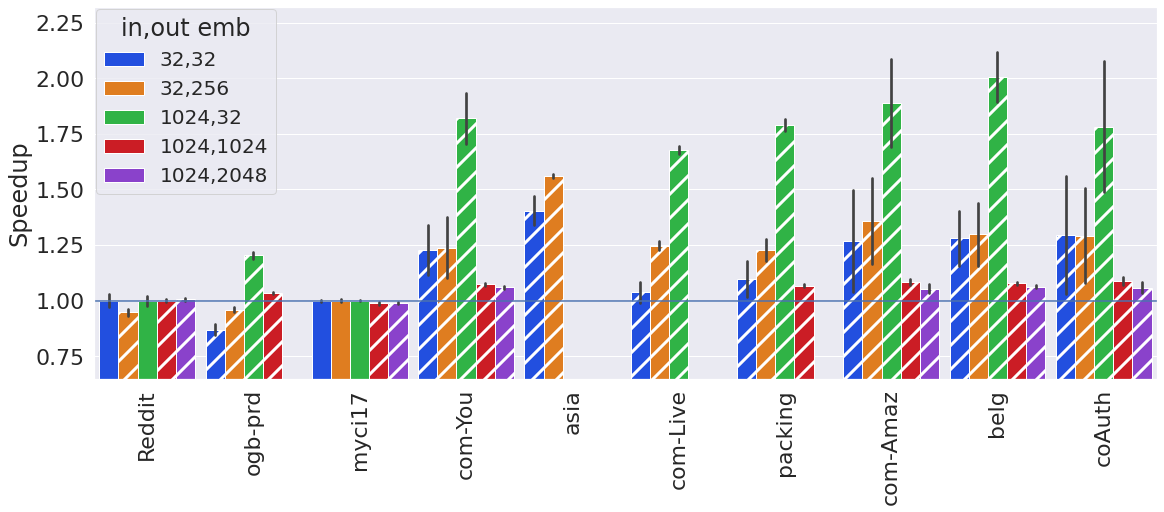
(a) GCN GPU Inference

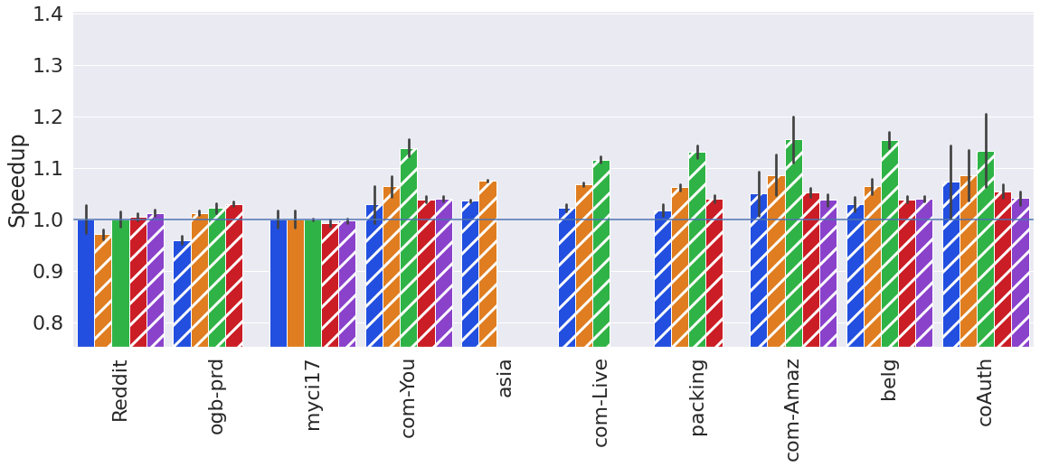
(b) GCN GPU Training

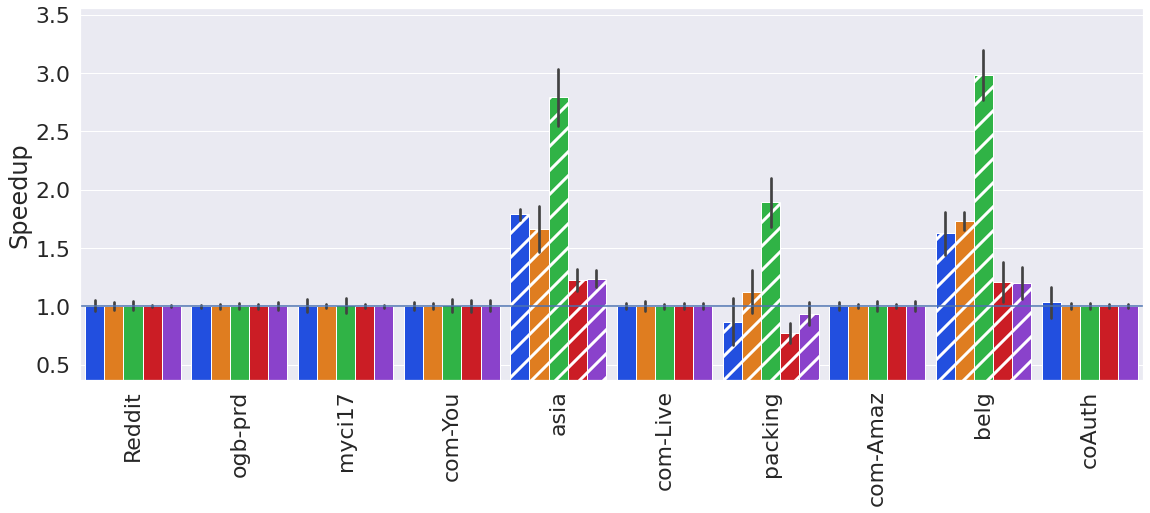
(c) GCN CPU Inference

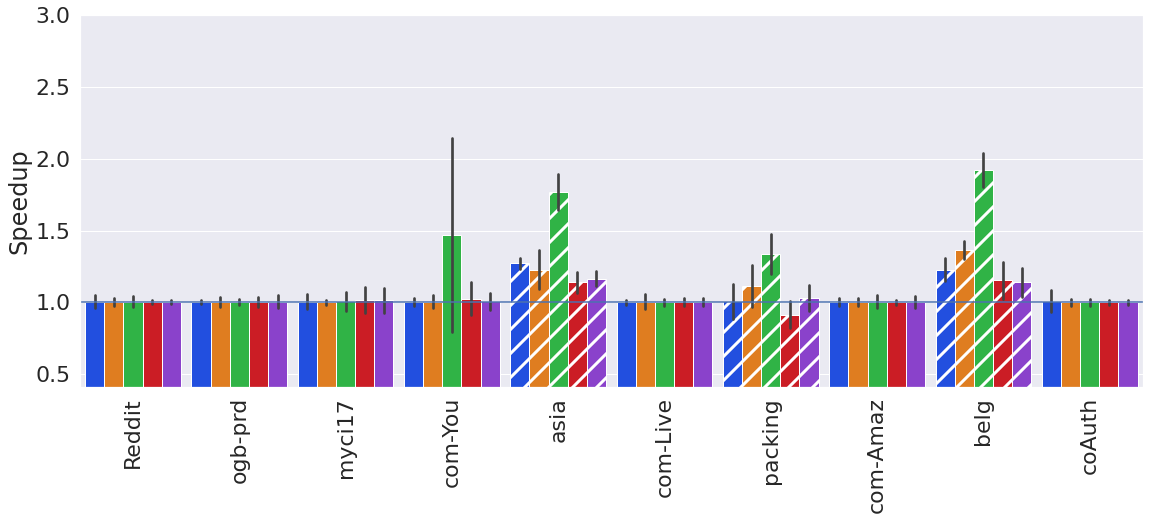
(d) GCN CPU Training

Figure 2. Speedups of SENSEi on DGL - GCN for 100 iterations. A hashed bar in the graph represents SENSEi deciding on precomputation is better, and for a solid bar, dynamic is decided to be better. The empty spaces in the GPU results represent failures due to OOM.

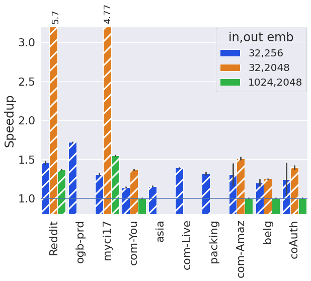
(a) GAT GPU Inference

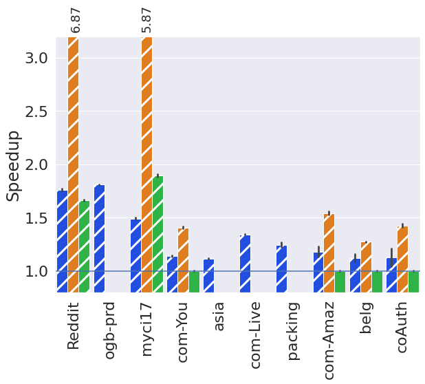
(b) GAT GPU Training

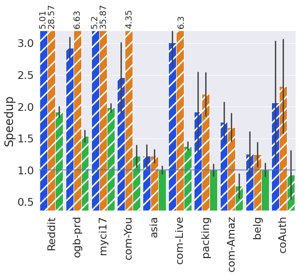
(c) GAT CPU Inference

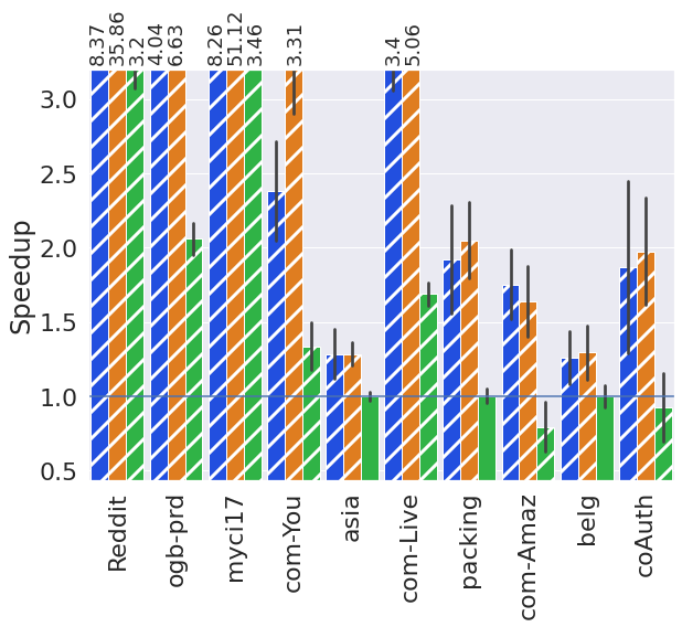
(d) GAT CPU Training

Figure 3. Speedups of SENSEi on DGL - GAT for 100 iterations. A hashed bar in the graph represents SENSEi deciding on recomputation is better, and for a solid bar, reuse is decided to be better. The empty spaces in the GPU results represent failures due to OOM.

Figures 2 and 3 present the speedups observed against the default execution of primitive compositions in DGL for GCN and GAT respectively for CPUs and GPUs under both inference and training. We run each configuration for 100 iterations to calculate the speedups. The summarized results of this evaluation are shown in Table 7. In summary, the results show that SENSEi is able to speedup most configurations by selecting the best primitive composition. Also note that SENSEi’s decisions vary based on the input graph and embedding sizes showing that it is important to decide the composition based on the input.

Table 7. Speedup summary of SENSEi on DGL

GNN	HW	Infer(I)	geomean	Max	Min	OOM
		Train(T)	spdup	spdup	spdup
GCN	GPU	I	$1.187\times$	$1.999\times$	$0.869\times$	7
		T	$1.04\times$	$1.154\times$	$0.96\times$
	CPU	I	$1.105\times$	$2.959\times$	$0.76\times$	0
		T	$1.06\times$	$1.912\times$	$0.903\times$
GAT	GPU	I	$1.44\times$	$5.69\times$	$1\times$	8
		T	$1.5\times$	$6.869\times$	$1\times$
	CPU	I	$2.307\times$	$35.866\times$	$0.73\times$	0
		T	$2.56\times$	$51.125\times$	$0.782\times$

For denser graphs used in GCN, SENSEi found DGL’s default method (dynamic) to be the most beneficial. However, SENSEi’s decisions differed for sparser graphs where the selection of the precompute primitive composition gave significant speedups. An example of a denser graph in this context would be Reddit possessing a density of $2\times 10^{-3}$, while a sparser graph would be asia_osm possessing a density of $1.78\times 10^{-7}$. This result is somewhat obvious for sparser graphs as the dense computation is much more significant. Thus, the dynamic primitive composition with its additional GEMM computations is sub-optimal, and running the precompute primitive composition would be more beneficial. SENSEi manages to correctly identify such points and make the correct decision between primitive composition choices. We observe higher speedups for the precompute primitive composition as the difference between input and output embedding sizes increases. This is attributed to the GEMM computation with the larger embedding size, which has a greater impact on the overall computation.

In GAT, we observe that for the majority of the configurations evaluated, SENSEi decided on the recomputation composition as the optimal. However, for larger embedding sizes of sparse graphs, the reuse composition was chosen as seen with belgium_osm for the embedding size of $1024,2048$. This is due to the dense computation becoming more prominent the sparser the graph is and the larger the embedding sizes are. In such situations, performing the additional GEMM computation to recompute the updated embeddings becomes too costly. In contrast, the more significant the sparse computation is as a bottleneck (as in denser graphs), the more speedup the GAT recomputation method would achieve. The accurate identification of the appropriate composition is enabled by the input sensitivity of SENSEi, which accounts for the significance of both the graph and the embedding sizes when making a decision. Furthermore, with increasing embedding sizes the speedups observed from recomputation are larger. This is clearly seen by the high speedups observed for both Reddit and mycielskian17 graphs for the embedding size of $32,2048$. This is due to the greater time savings achieved from performing the aggregation with the smaller embedding size.

The slowdowns observed in the evaluations were due to SENSEi making incorrect choices. Although SENSEi is not perfect, slowdowns are observed in only 6.2% out of all the configurations evaluated. Furthermore, these slowdowns are only up to $1.36\times$ of the original DGL execution.

We observe that speedups for GAT are much greater than GCN. This is because the differences in primitive compositions for GCN are mainly based on the balancing of memory use and computation to achieve the best performance, while the primitive compositions of GAT directly lead to significant reductions in computation. The speedups observed during inference are greater than training in GCNs. The additional computations that occur during the training process that we do not optimize for could be the reason for this, as the contribution to the overall speedup is less compared to inference. However, the opposite is observed for GAT, where larger speedups for training are seen. This could point to the recomputation primitive composition affecting the backward pass as well, resulting in an overall speedup. Although the aforementioned observation highlights general trends, making the correct choice is non-trivial. We present further analysis in Section 6.6.

6.4. Synergy with other optimizations

(a) CPU/C++ build of GCN for embeddings of input-32/output-32.

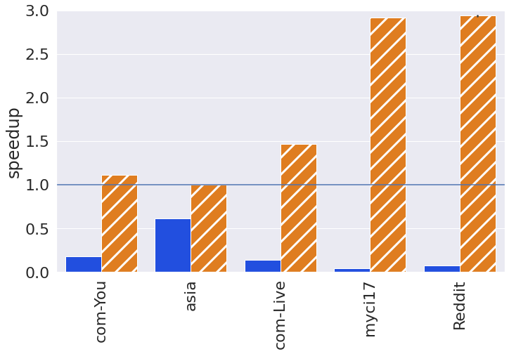
(b) CPU/C++ build of GAT for embeddings of input-32/output-256.

Figure 4. Speedups on OPT execution system against default DGL and OPT with SENSEi. A hashed bar represents SENSEi deciding on precomputation or recomputation is better, and a solid bar represents SENSEi deciding on dynamic or reuse is better for GCN and GAT respectively.

We evaluated SENSEi’s decision-making capabilities on the OPT execution system. Here, given an optimized execution, SENSEi decides the primitive composition to execute. We used a subset of the graphs and embedding sizes from Section 6.3 as points to show the synergy between the traditional sparse optimizations and the primitive compositions. Figure 4 shows the comparisons against both the default DGL execution, as well as the optimized implementation with SENSEi’s primitive composition decisions.

We observe sizable speedups compared to DGL from the classical optimizations alone. These speedups range from a minimum $1.82\times$ of up to $4.881\times$, and a minimum of $1.63\times$ up to $21.554\times$ over DGL for GCN, and GAT respectively. These speedups showcase the performance of the optimized code over DGL.

We see that the trend of speedups observed from the primitive compositions still hold with a similar speedup pattern to what was observed when getting decisions for DGL from SENSEi. Overall, these are speedups of upto $1.218\times$ and upto $2.94\times$ for GCN and GAT. We do not observe speedups from SENSEi’s decisions in certain configurations due to the default dynamic composition being selected as the best. Also, note that, compared to the speedups observed due to the compositions in DGL, we see lower speedups for GCN (asia_osm for embedding sizes of $32,32$ is observed to be $1.6\times$ in DGL and $1.2\times$ in OPT for precompute), and GAT (Reddit for embedding sizes of $32,256$ is observed to be $5.7\times$ in DGL and $2.93\times$ in OPT for recompute). The difference in primitive kernels as well as the additional optimizations applied may reduce the gains seen from changing the primitive compositions.

6.5. Overheads of SENSEi

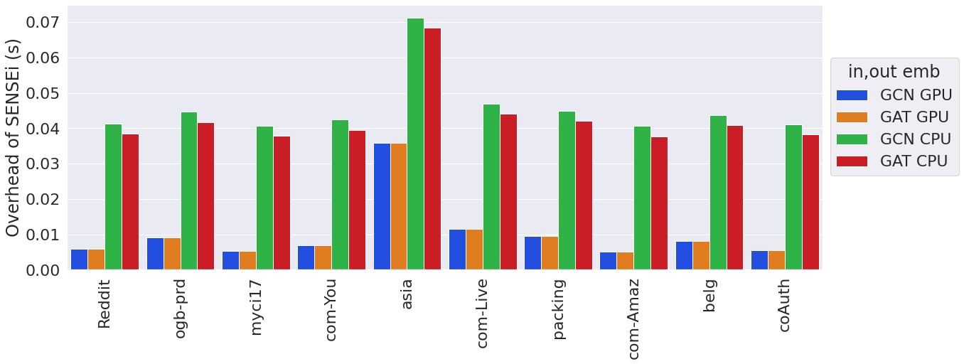
Figure 5. Overheads from SENSEi in DGL per graph

SENSEi has an overhead of the additional graph inspection and model decision-making as shown by Figure 5. We run the XGBoost model of SENSEi on the evaluation architecture. Because XGBoost can utilize a GPU when available, it can use it to accelerate its decision speed compared to a CPU-only system. Apart from the model decision time, which will remain the same for each input considered, the graph inspection time to identify the characteristics of the graph adds to the overhead as well. The embedding size does not influence the overhead but does affect the iteration time. Thus, we present the raw overhead in terms of time in Figure 5 for better clarity. The iteration times for GCN and GAT range from 0.001s to 10s.

The categorization of each overhead percentage compared to its iteration time is presented in Table 8. Here, we consider all GNN configurations evaluated (graph $\times$ feature sizes $\times$ model) to arrive at a total of 145 configurations. Only a small portion of the configurations result in an overhead higher than its iteration time. Even among these, the maximum overhead is limited to $5.69\times$ across both hardware platforms.

Table 8. Overheard of SENSEi on DGL in iterations

HW	Overhead in iterations
	$<0.1$	$<0.5$	$<1$	$<2$	$>=2$	max
GPU	26	19	9	7	4	$2.93\times$
CPU	43	17	10	4	6	$5.69\times$

6.6. Learned model of SENSEi and feature importance

We compare the geomean speedup of the optimal configuration (Oracle Geomean), with the decisions made by SENSEi (model). In addition, we evaluate decisions made by an oracle that is capable of selecting the best primitive composition considering only the underlying hardware architecture (arch), embedding sizes (emb), or the input graph (graph) independently for each GCN and GAT. For example, considering the oracle for graph, if the recompute composition is most often the best for GAT on any embedding size and hardware for a given graph, then the oracle will always choose the recompute option for that graph for all architectures and embedding sizes. The result of this analysis is presented in Table 9, and shows the benefit of using a learned system in SENSEi. Although the impact of the architecture as well as embedding sizes cannot be denied through these results, the graph-based oracles come closest in terms of accuracy to SENSEi. However, the graph feature corresponding to selecting the correct primitive composition is not the most obvious, which is density. This is supported by the contrastingly different observations for ogbn-products and com-Amazon with similar density.

Considering the feature importance of the XGBoost models shown in Figure 6, it is possible to see that multiple features contribute to making the final decision. The top four features for both composition selectors are output embedding sizes, number of rows, number of nnzs, and graph density. However, how they contribute to the final decision does not seem straightforward to interpret.

Table 9. Model performance of SENSEi against basic heuristics

GNN	Oracle	SENSEi	Oracle Decisions
	Geomean		arch	emb	graph
GCN	1.185	1.144	1.075	0.871	1.116
GAT	1.939	1.923	1.811	1.815	1.811

These observations support that making the correct decision is non-trivial and requires a combination of multiple factors as well as a way to identify the characteristics that contribute to the correct decision. With a data-driven approach, a correct decision can be identified by training an appropriate model as that has been done with SENSEi. Instead of manually searching to find an ideal heuristic in each scenario, scripted data collection and training can decide the adaptability and accuracy of the results.

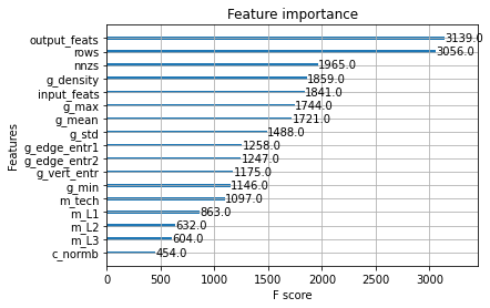
(a) Feature importance for GCN

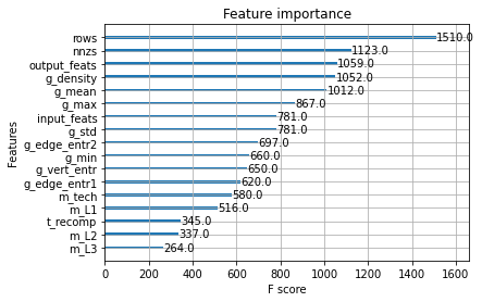
(b) Feature importance for GAT

Figure 6. Feature importance of XGBoost models

7. Discussion

Generalizability of compositions

Although we specialized the primitive composition choices presented to particular GNN models, it is possible to generalize them to patterns observed in GNNs in general. The choice between precomputation and dynamic compositions could emerge in a situation where re-associativity of the computations considered leads to multiple dense-sparse primitive choices. Similarly, the choice between reuse and recomputation might arise at a point where an update computation on the same embedding ($H^{(l-1)}\cdot W^{(l)}$) is required multiple times. An example of a possible situation would be the GATv2 model (brody2022:gatv2, ).

Approximate GNN optimization techniques

In Section 6.4, we presented how the primitive compositions give synergistic benefits for traditional sparse optimizations. However, especially when considering scaling to larger graphs, there are multiple techniques in the GNN domain to reduce the overall computation. One such method is sampling, which would alter the input graph structure in some manner which SENSEi relies on. In situations where sampling does not change the sparsity pattern of the graph, then we can apply SENSEi to a sampled graph and then reuse its decisions.

8. Related work

Input Sensitive Systems

There has been limited work on systems strictly dedicated to optimizing GNNs based on input. GNNAdvisor (ding-gnnadvisor, ) is one such system where based on the input graph, a set of handcrafted functions are used to identify optimization opportunities. Its optimizations are tailored towards GPU-based sparse executions and the thresholds are heuristically set instead of being learned. (qiu:xgboost_format_selection_GNN, ) is quite similar to SENSEi as it proposes a machine-learning model to predict the best data representation for sparse operations in GNNs. Similarly, WISE (serif:wise, ) proposes a machine-learning solution to select the best data representation for SpMV. Works such as ASpT (ASpT, ) and LAV (serif:LAV, ) present input-aware sparse optimizations that introduce new sparse representations and are coupled with specialized executions. Focusing on graph operations in general, (GPUGraphAutotuner, ) proposes a solution quite similar to SENSEi wherein it presents a learned solution that performs sparse optimizations based on characteristics of the input graph. However, this, along with the aforementioned solutions, considers optimizations primarily only on sparse computations. By not considering the input-aware interplay of sparse and dense in the context of GNNs, multiple optimization opportunities are missed as identified by SENSEi. In contrast, (yan:feat_op_GNN_selection, ), (which we include in SENSEi), considers the interplay between sparse and dense computation, but focuses on deciding solely based on the input and output embedding size. Instead, SENSEi jointly considers the embedding sizes, the input graph and the underlying hardware architecture.

GNN optimizations

Graphiler (graphiler, ), and SeaStar (yidi2021:seastar, ) present compiler-based solutions that allow GNN models written in user-defined functions to be converted into highly optimized code based on the computations specified. (zhang2021understanding, ) also considers recomputation as an optimization. However, this is in terms of reducing memory utilization of the end-to-end GNN training process and overlooks performance optimizations possible through recomputation as SENSEi does. FusedMM (rahman2020fusedmm, ) and Graphite (josep2022:graphite, ) also present GNN kernel fusions albeit specifically on CPU. Notably, the fusion proposed by Graphite is between sparse and dense data components. This relates to SENSEi as it considers the interplay between sparse and dense data. As SENSEi offers a method of selecting optimizations given the input, all optimizations presented in such systems would compose with SENSEi.

9. Conclusion

In this work, we propose different primitive compositions for executing two popular GNN models. To automatically make the correct decision between these compositions, we present SENSEi, an input-sensitive decision maker for selecting GNN primitive compositions that caters its decision based on the input graph, embedding sizes, and hardware architecture. SENSEi allows users to attain speedups over the default execution in DGL, a popular GNN framework over a wide range of graphs and embedding sizes in both CPUs and GPUs.

10. Acknowledgements

This work is supported by ACE, one of the seven centers in JUMP 2.0, a Semiconductor Research Corporation (SRC) program sponsored by DARPA.

References

- [1] Shaked Brody, Uri Alon, and Eran Yahav. How attentive are graph attention networks? In International Conference on Learning Representations, 2022.
- [2] Tianqi Chen and Carlos Guestrin. XGBoost. In Proceedings of the 22nd ACM SIGKDD International Conference on Knowledge Discovery and Data Mining. ACM, aug 2016.
- [3] Timothy A. Davis. Algorithm 1000: Suitesparse:graphblas: Graph algorithms in the language of sparse linear algebra. ACM Trans. Math. Softw., 45(4), dec 2019.
- [4] Timothy A. Davis and Yifan Hu. The university of florida sparse matrix collection. ACM Trans. Math. Softw., 38(1), dec 2011.
- [5] Matthias Fey and Jan E. Lenssen. Fast graph representation learning with PyTorch Geometric. In ICLR Workshop on Representation Learning on Graphs and Manifolds, 2019.
- [6] Zhangxiaowen Gong, Houxiang Ji, Yao Yao, Christopher W. Fletcher, Christopher J. Hughes, and Josep Torrellas. Graphite: Optimizing graph neural networks on cpus through cooperative software-hardware techniques. In Proceedings of the 49th Annual International Symposium on Computer Architecture, ISCA ’22, page 916–931, New York, NY, USA, 2022. Association for Computing Machinery.
- [7] Changwan Hong, Aravind Sukumaran-Rajam, Israt Nisa, Kunal Singh, and P. Sadayappan. Adaptive sparse tiling for sparse matrix multiplication. In Proceedings of the 24th Symposium on Principles and Practice of Parallel Programming, PPoPP ’19, page 300–314, New York, NY, USA, 2019. Association for Computing Machinery.
- [8] Weihua Hu, Matthias Fey, Marinka Zitnik, Yuxiao Dong, Hongyu Ren, Bowen Liu, Michele Catasta, and Jure Leskovec. Open graph benchmark: Datasets for machine learning on graphs. arXiv preprint arXiv:2005.00687, 2020.
- [9] Kezhao Huang, Jidong Zhai, Zhen Zheng, Youngmin Yi, and Xipeng Shen. Understanding and bridging the gaps in current gnn performance optimizations. In Proceedings of the 26th ACM SIGPLAN Symposium on Principles and Practice of Parallel Programming, PPoPP ’21, page 119–132, New York, NY, USA, 2021. Association for Computing Machinery.
- [10] Zhihao Jia, Sina Lin, Mingyu Gao, Matei Zaharia, and Alex Aiken. Improving the accuracy, scalability, and performance of graph neural networks with roc. In Proceedings of Machine Learning and Systems 2020, pages 187–198. 2020.
- [11] Wengong Jin, Kevin Yang, Regina Barzilay, and Tommi Jaakkola. Learning multimodal graph-to-graph translation for molecule optimization. In International Conference on Learning Representations, 2019.
- [12] Sam Kaufman, Phitchaya Phothilimthana, Yanqi Zhou, Charith Mendis, Sudip Roy, Amit Sabne, and Mike Burrows. A learned performance model for tensor processing units. In A. Smola, A. Dimakis, and I. Stoica, editors, Proceedings of Machine Learning and Systems, volume 3, pages 387–400, 2021.
- [13] Thomas N. Kipf and Max Welling. Semi-supervised classification with graph convolutional networks. CoRR, abs/1609.02907, 2016.
- [14] Jérôme Kunegis and Julia Preusse. Fairness on the web: Alternatives to the power law. In Proceedings of the 4th Annual ACM Web Science Conference, WebSci ’12, page 175–184, New York, NY, USA, 2012. Association for Computing Machinery.
- [15] Chen Liang, Ziqi Liu, Bin Liu, Jun Zhou, Xiaolong Li, Shuang Yang, and Yuan Qi. Uncovering insurance fraud conspiracy with network learning. In Proceedings of the 42nd International ACM SIGIR Conference on Research and Development in Information Retrieval, SIGIR’19, page 1181–1184, New York, NY, USA, 2019. Association for Computing Machinery.
- [16] Ziqi Liu, Chaochao Chen, Xinxing Yang, Jun Zhou, Xiaolong Li, and Le Song. Heterogeneous graph neural networks for malicious account detection. CIKM ’18, page 2077–2085, New York, NY, USA, 2018. Association for Computing Machinery.
- [17] Lingxiao Ma, Zhi Yang, Youshan Miao, Jilong Xue, Ming Wu, Lidong Zhou, and Yafei Dai. Neugraph: parallel deep neural network computation on large graphs. In 2019 USENIX Annual Technical Conference (USENIXATC 19), pages 443–458, 2019.
- [18] Ke Meng, Jiajia Li, Guangming Tan, and Ninghui Sun. A pattern based algorithmic autotuner for graph processing on gpus. In Proceedings of the 24th Symposium on Principles and Practice of Parallel Programming, PPoPP ’19, page 201–213, New York, NY, USA, 2019. Association for Computing Machinery.
- [19] Adam Paszke, Sam Gross, Soumith Chintala, Gregory Chanan, Edward Yang, Zachary DeVito, Zeming Lin, Alban Desmaison, Luca Antiga, and Adam Lerer. Automatic differentiation in pytorch. 2017.
- [20] Shenghao Qiu, Liang You, and Zheng Wang. Optimizing sparse matrix multiplications for graph neural networks. In Xiaoming Li and Sunita Chandrasekaran, editors, Languages and Compilers for Parallel Computing, pages 101–117, Cham, 2022. Springer International Publishing.
- [21] Md Rahman, Majedul Haque Sujon, Ariful Azad, et al. Fusedmm: A unified sddmm-spmm kernel for graph embedding and graph neural networks. In 35th Proceedings of IEEE IPDPS, 2021.
- [22] John Thorpe, Yifan Qiao, Jonathan Eyolfson, Shen Teng, Guanzhou Hu, Zhihao Jia, Jinliang Wei, Keval Vora, Ravi Netravali, Miryung Kim, and Guoqing Harry Xu. Dorylus: Affordable, scalable, and accurate GNN training with distributed CPU servers and serverless threads. In 15th USENIX Symposium on Operating Systems Design and Implementation (OSDI 21), pages 495–514. USENIX Association, July 2021.
- [23] Wen Torng and Russ B. Altman. Graph convolutional neural networks for predicting drug-target interactions. Journal of Chemical Information and Modeling, 59(10):4131–4149, 10 2019.
- [24] Petar Veličković, Guillem Cucurull, Arantxa Casanova, Adriana Romero, Pietro Liò, and Yoshua Bengio. Graph attention networks. In International Conference on Learning Representations, 2018.
- [25] Minjie Wang, Lingfan Yu, Da Zheng, Quan Gan, Yu Gai, Zihao Ye, Mufei Li, Jinjing Zhou, Qi Huang, Chao Ma, Ziyue Huang, Qipeng Guo, Hao Zhang, Haibin Lin, Junbo Zhao, Jinyang Li, Alexander Smola, and Zheng Zhang. Deep graph library: Towards efficient and scalable deep learning on graphs, 2019.
- [26] Yuke Wang, Boyuan Feng, Gushu Li, Shuangchen Li, Lei Deng, Yuan Xie, and Yufei Ding. GNNAdvisor: An adaptive and efficient runtime system for GNN acceleration on GPUs. In 15th USENIX Symposium on Operating Systems Design and Implementation (OSDI 21), pages 515–531. USENIX Association, July 2021.
- [27] Jaeyeon Won, Charith Mendis, Joel Emer, and Saman Amarasinghe. Waco: Learning workload-aware co-optimization of the format and schedule of a sparse tensor program. In Proceedings of the seventeenth international conference on Architectural Support for Programming Languages and Operating Systems, 2023.
- [28] Yidi Wu, Kaihao Ma, Zhenkun Cai, Tatiana Jin, Boyang Li, Chenguang Zheng, James Cheng, and Fan Yu. Seastar: Vertex-centric programming for graph neural networks. In Proceedings of the Sixteenth European Conference on Computer Systems, EuroSys ’21, page 359–375, New York, NY, USA, 2021. Association for Computing Machinery.
- [29] Zhiqiang Xie, Minjie Wang, Zihao Ye, Zheng Zhang, and Rui Fan. Graphiler: Optimizing graph neural networks with message passing data flow graph. In D. Marculescu, Y. Chi, and C. Wu, editors, Proceedings of Machine Learning and Systems, volume 4, pages 515–528, 2022.
- [30] Mingyu Yan, Zhaodong Chen, Lei Deng, Xiaochun Ye, Zhimin Zhang, Dongrui Fan, and Yuan Xie. Characterizing and understanding gcns on gpu. IEEE Computer Architecture Letters, 19:22–25, 2020.
- [31] Serif Yesil, Azin Heidarshenas, Adam Morrison, and Josep Torrellas. Speeding up spmv for power-law graph analytics by enhancing locality and vectorization. In SC20: International Conference for High Performance Computing, Networking, Storage and Analysis, pages 1–15, 2020.
- [32] Serif Yesil, Azin Heidarshenas, Adam Morrison, and Josep Torrellas. Wise: Predicting the performance of sparse matrix vector multiplication with machine learning. In Proceedings of the 28th ACM SIGPLAN Annual Symposium on Principles and Practice of Parallel Programming, PPoPP ’23, page 329–341, New York, NY, USA, 2023. Association for Computing Machinery.
- [33] Hengrui Zhang, Zhongming Yu, Guohao Dai, Guyue Huang, Yufei Ding, Yuan Xie, and Yu Wang. Understanding gnn computational graph: A coordinated computation, io, and memory perspective. 4:467–484, 2022.
- [34] Muhan Zhang and Yixin Chen. Link prediction based on graph neural networks. In Advances in Neural Information Processing Systems, pages 5165–5175, 2018.
- [35] Yue Zhao, Jiajia Li, Chunhua Liao, and Xipeng Shen. Bridging the gap between deep learning and sparse matrix format selection. In Proceedings of the 23rd ACM SIGPLAN Symposium on Principles and Practice of Parallel Programming, PPoPP ’18, page 94–108, New York, NY, USA, 2018. Association for Computing Machinery.