Boson subtraction as an alternative to fusion gates for generating graph states

Abstract

Qubit graph states are essential computational resources in measurement-based quantum computations (MBQC). The most well-known method to generate graph states in optics is to use fusion gates, which in many cases require expensive entangled resource states. In this work, we propose an alternative approach to generate graph states based on the graph picture of linear quantum networks (LQG picture), through which we can devise schemes that generate caterpillar graph states with boson subtractions. These subtraction schemes correspond to efficient heralded optical setups with single-photon sources and more flexible measurement elements than fusion gates. Caterpillar graph states encompass various useful graph structures for one-way quantum computing, such as linear graphs, star graphs, and networks of star graphs. We can exploit them as resources for generating cluster states using conventional Type II fusion gates. Our results demonstrate that the boson subtraction operator is a more general concept that encompasses and can therefore optimize fusion gates.

I Introduction

Graph states are multipartite genuinely entangled states represented by graphs, where vertices and edges correspond to qubits and their nonlocal controlled-Z (CZ) interactions hein2004multiparty; hein2006entanglement. Graph states play a crucial role in quantum computation nielsen2006cluster and communication bell2014experimental. Particularly, they serve as resources in measurement-based quantum computing and quantum error-corrections raussendorf2012quantum; browne2016one. There have been several attempts to generate various types of graph states both probabilistically uskov2015resource; istrati2020sequential; singh2022optical; zhang2022loss and deterministically schwartz2016deterministic; russo2019generation; thomas2022efficient; shapourian2023modular; hilaire2023near.

The most commonly used method for generating graph states in optics is to apply fusion gates to multiple entangled states of small parties for generating graph states of larger parties browne2005resource; varnava2006loss; varnava2008good; li2015resource; bartolucci2023fusion; lee2023graph. The fusion-based method offers a convenient theoretical framework due to the direct correspondence between CZ gates of qubits and fusion gates of photons. However, several obstacles hinder the practical graph state generation based on the fusion gates. They generally require a significant amount of entangled states as resources, which are expensive and challanging to control in the process of generating useful resource states of larger size.

On the other hand, there exists another graphical approach to provide a systematic method for generating entangled states with quantum systems of single-particle sources and linear operations, which we term linear quantum networks). Refs. chin2021graph; chin2022graph introduced a graph picture of linear quantum networks (LQG picture), which furnishes handy mathematical tools that simplify the design of entanglement generating circuits. Ref. chin2021graph suggested an undirected bipartite graph picture of linear quantum networks (see Appendix A for a glossary in graph theory), which can be always transformed into unipartite directed graphs. In this picture, necessary conditions for generating multipartite genuine entangled states with postselection are found and used for designing LQS schemes for several entangled states. Ref. chin2022graph generalized this approach to embrace subtraction operators, based on which heralded schemes of linear quantum networks for generating crucial entangled states (qubit GHZ, qubit W, and qudit GHZ states) are found chin2023graphs.

The successful application of the LQG picture to the generation of essential multipartite entangled states naturally gives rise to an interesting and crucial question: Can we use the LQG picture to find a systematic way to generate graph states with single-particle sources? Since single photons sources can be created near-deterministically with high indistinguishability in quantum dot systems somaschi2016near; couteau2023applications and controlled with less errors, heralded schemes constructed based on the LQG picture would generate graph states in a more feasible manner.

Our study presents a partial but remarkable answer to this question. We propose a LQG graph structure, which we name the central path digraph, that directly corresponds to heralded schemes for generating arbitrary caterpillar graph states in linear quantum networks. Caterpillar graph states encompass various useful graph states for one-way quantum computing such as linear graphs, star graphs, and networks of star graphs. In the optical realization of our scheme, we can generate the heralded graph states with simple optical circuits made of single photon sources, polarizing beam splitters (PBSs), and half-wave plates (HWPs) chin2023graphs. Other than the advantage that our heralded schemes do not need entangled sources, we will also show that they generate the same caterpillar graph states with higher success probability and significantly less photons. The caterpillar states generated in this more efficient way can be used to generate cluster states with additional fusion gates.

II Directed unipartite graph representation $G_{du}$ of the sculpting protocol

Sculpting operators	Sculpting bigraphs
in bosonic systems	$G_{ub}=(U\cup V,E)$
Spatial modes $j$	Labelled circles () $\in$ $U$
$\hat{A}^{(l)}$	Unlabelled dots ($\bullet$) $\in$ $V$
Spatial distributions of $\hat{A}^{(l)}$	Edges $\in$ $E$
Probability amplitude $\alpha_{j}^{(l)}$	Edge weight $\alpha_{j}^{(l)}$
Internal state $\psi_{j}^{(l)}$	Edge weight $\psi_{j}^{(l)}$

Table 1: Correspondence relations between sculpting operators and sculpting bigraphs

We require two steps to map heralded schemes of linear quantum systems into our graph picture chin2022graph; chin2023graphs. First, we employ the sculpting protocol karczewski2019sculpting, which generates entangled states by taking spatially overlapped $N$ single-boson subtraction operators (dubbed “sculpting operators”) to a $2N$ boson initial state. And correspondence relations between elements in the sculpting protocol and bipartite graphs were presented in Ref. chin2022graph, by which all the operations in the sculpting protocols are translated to the bipartite graphs (dubbed “sculpting bigraphs”). Second, since linear bosonic systems with heralding detectors realize sculpting operators with concrete translation rules chin2023graphs, we can design $N$-partite genuine entanglement generation schemes based on the graph approach. In other words, once we find a sculpting bigraph that generates a specific type of entanglement, we can directly design heralded linear quantum schemes that generates the same entanglement.

Here we summarize the correspondence relations bewteen sculpting operator elements and graph elements of LQG picture introduced in Ref. chin2022graph (see Appendix B for a review on the protocol) and explain two graph representations for the same sculpting protocol, the undirected bipartite graph representation (bigraph representation for short, $G_{ub}$) and directed unipartite graph representation (digraph representation for short, $G_{du}$). The latter will be mostly used in this work to present the schemes that generate caterpillar graph states. While the bigraph representation $G_{ub}$ describes sculpting protocols more intuitively, the digraph representation $G_{du}$ reveals the information on the genuine entanglement of given schemes more manifestly chin2021graph, which we will explain here.

The bigraph mapping of sculpting operators $\hat{A}_{N+K}$ (the definition is given in Eq. (2)) is enumerated in Table I chin2022graph. In this paper, the internal states $\{|+\rangle,|-\rangle,|0\rangle,|1\rangle\}$ ($|0\rangle=\frac{1}{\sqrt{2}}(|+\rangle+|-\rangle)$, $|1\rangle=\frac{1}{\sqrt{2}}(|+\rangle-|-\rangle)$) are expressed as edge colors {Solid Black, Dashed Black, Red, Blue} for simplicity.

In the bigraph picture, the sculpting bigraph are set so that the final state $|\Psi\rangle_{fin}$ is the superposition of the perfect matchings (PMs) of the sculpting bigraph by the no-bunching condition (Property 1 of Ref. chin2022graph). It is generally challanging to control edge weights for a sculpting bigraph to satisfy this property and generate genuine entanglement simultaneously. However, there exists a specifically convenient type of bigraphs that automatically satisfy the no-bunching condition, which are dubbed effective perfect matching bigraphs (EPM bigraphs):

Definition 1.

(EPM bigraphs chin2022graph) If all the edges of a bigraph attach to the circles as one of the following forms

$$\begin{gathered}\includegraphics[width]{EPM_bigraph}\end{gathered},$$

$$(\{|+\rangle,|-\rangle,|0\rangle,|1\rangle\}$$

$$~~~=\{\textrm{SolidBlack, DashedBlack, Red, Blue}\}$$ (2)

where $n$ is the number of edges and the probability amplitude edge weights are all non-zero, then it is an effective perfect matching bigraph (EPM bigraph).

We can easily see that if a sculpting bigraph is an EPM bigraph, then the final state becomes a superposition of the PMs of the bigraph (Property 2 of Ref. chin2022graph). Ref. chin2022graph suggests several sculpting EPM bigraphs that generates multipartite genuine entanglement. For example, a bigraph for the $N$-partite qubit GHZ state is given by

(3)

(we choose a simplified notation, i.e., all the edges from the same dot has the same absolute value of probability amplitude when edge weights are omitted), which corresponds to a sculpting operator

$$\hat{A}_{N} =\frac{1}{\sqrt{2^{N}}}({\hat{a}}_{1,0}+{\hat{a}}_{2,1})({\hat{a}}_{2,0}+{\hat{a}}_{3,1})\cdots$$

$$~~~\times({\hat{a}}_{N-1,0}+{\hat{a}}_{N,1})({\hat{a}}_{N,0}+{\hat{a}}_{1,1})$$ (4)

by Table I. The above bigraph is an EPM bigraph which is made of the first one in (1).

The sculpting bigraphs intuitively describe the essential feature of the operators and render the direct transformation rule from sculpting operators to linear optical circuits chin2022graph. However, when the number of subsystems increases and the operator becomes less symmetric, it is hard to read the entanglement property with those bigraphs. In that case, the digraph representation $G_{du}$ of operators has the advantage of manifestly verifying the entanglement structure and the perfect matchings in the final state. A digraph for a given bigraph is defined as follows:

Definition 2.

(From a bigraph to a digraph)

For a balanced bigraph $G_{ub}=(U\cup V,E)$, its digraph counterpart $G_{du}=(W,F)$ is obtained by mapping two vertices $i$ ($\in U$) and $i^{\prime}$ ($\in V$) into a vertex $i^{\prime\prime}$ ($\in W$), and a undirected edge $(i,j^{\prime})$ ($\in E$) to a directed edge $(i^{\prime\prime}\to j^{\prime\prime})$ ($\in F$).

In the above definition, the unlabelled vertices in $V$ are temporarily labelled for the convenience. Intuitively, a bigraph is obtained by merging one circle in $U$ and one dot in $V$ and impose a direction from the dot to the circle to preserve the distinction between dots and circles. Then the digraph mapping of sculpting operators is given as Table II. We can achieve the same mapping using the fact that one adjacency matrix can construct both a bigraph and a digraph brualdi1980bigraphs (see Sec. 2.2 of Ref. chin2021graph for a more specific explanation to our case). From now on, a digraph that corresponds to a sculpting bigraph, hence to a sculpting operator, is called a sculpting digraph. The GHZ sculpting digraph is drawn from (3) as

$$\includegraphics[width]{GHZ2}.$$ (5)

Sculpting operators	Sculpting digraphs
in bosonic systems	$G_{du}=(W,E)$
Spatial modes $j$	Circles () $\in$ $W$
$\hat{A}^{(l)}$	Circles () $\in$ $W$
Spatial distributions of $\hat{A}^{(l)}$	Directed edges $\in$ $E$
Probability amplitude $\alpha_{j}^{(l)}$	Edge weight $\alpha_{j}^{(l)}$
Internal state $\psi_{j}^{(l)}$	Edge weight $\psi_{j}^{(l)}$

Table 2: Correspondence relations between sculpting operators and sculpting digraphs. Note that both $N$ spatial modes and $N$ subtraction operators $\hat{A}^{(l)}$ are denoted as circles. Since all the subtraction operators are identical, the assignment of $l$ to each subtraction operator is arbitrary and the mapping from a bigraph to a digraph is not unique.

EPM digraphs are defined in combination of Definitions 1 and 2 as follows:

Definition 3.

(EPM digraphs) EPM digraphs are those whose edges come to the circles as one of the following forms

$$\begin{gathered}\includegraphics[width]{EPM_digraph}\end{gathered}.$$

There are two useful properties that sculpting digraphs have: First, in a sculpting digraph, a cycle (a closed path other than loops) corresponds to an independent PM in the bigraph counterpart. Therefore, when a bigraph has a complicated structure in a large system, the digraph representation is much easier to verify the PMs (Sec. 2.4 of Ref. chin2021graph). And one PM in the bigraph representation is expressed as a directed PM in the digraph representation (see Appendix A for the definition). Second, we can find necessary conditions for a sculpting operator to generate genuine multipartite entanglement with the digraph representation, which is elucidated in the following theorem:

Theorem 1.

For a sculpting operator to generate a genuinely entangled state, i) each vertex in its corresponding $G_{du}$ must have more than two incoming edges of different colors, and ii) all the vertices in it are strongly connected to each other.

This theorem is first proven in Ref. chin2021graph for the multipartite entanglement generation of identical particles with postselection, which directly holds for the sculpting protocol as well. Therefore, for an EPM digraph to generate multipartite genuine entanglement, it must satisfy the two conditions in Theorem 1. It provides a powerful guideline to find sculpting operators to generate multipartite genuinely entangled states. We can find such operators by drawing EPM digraphs so that they fulfill the two necessary conditions in the first place and check the final state by verifying their directed PMs, which immensely diminishes the number of cases we have to consider.

One can check all the sculpting EPM bigraphs given in Ref. chin2022graph satisfy conditions i) and ii). The digraph representation $G_{du}$ is particularly useful for the schemes in this work whose sculpting operators have complicated structure of ancillary systems, as we will see in the next section.

III Sculpting digraphs for Caterpillar graph states

Caterpillar graph states are those whose qubits are connected with Controlled-Z (CZ) gates (see Appendix C for its definition and identities) in the shape of a caterpillar (a tree graph in which every vertex is on the central path or one edge away from the path). The definitions and more detailed explanations on the caterpillar graph states are given in Appendix D.

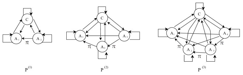
Here we present a group of sculpting digraphs that generate caterpillar graph states with a central path of an arbitrary length. With our scheme, any caterpillar graph state with a central path of length $l$ is generated by sculpting protocol with $l+1$ ancillary modes. The ancillary modes play the role of the central path that connects several star graphs, which is dubbed the central path digraph $P^{(l)}$:

Definition 4.

(Central path digraph) A central path digraph $P^{(l)}$ of $(l+2)$ vertices $\{C,A_{1},A_{2},\cdots,A_{n},A_{l+1}\}$ is a digraph whose adjacency matrix is defined in an iterative manner as follows:

$$P^{(1)}= \left[\begin{array}[]{ccc}a_{CC}&a_{CA_{1}}&a_{CA_{2}}\\ a_{A_{1}C}&a_{A_{1}A_{1}}&a_{A_{1}A_{2}}\\ a_{A_{2}C}&a_{A_{2}A_{1}}&a_{A_{2}A_{2}}\end{array}\right]=\left[\begin{array}[]{ccc}1&1&1\\ 1&1&0\\ 1&-1&1\\ \end{array}\right],$$

$$P^{(l)}= \left[\begin{array}[]{ccccc}a_{CC}&a_{CA_{1}}&a_{CA_{2}}&\cdots&a_{CA_{l+1}}\\ a_{A_{1}C}&a_{A_{1}A_{1}}&a_{A_{1}A_{2}}&\cdots&a_{A_{1}A_{l+1}}\\ \vdots&\vdots&\vdots&\ddots&\vdots\\ a_{A_{l+1}C}&a_{A_{l+1}A_{1}}&a_{A_{l+1}A_{2}}&\cdots&a_{A_{l+1}A_{l+1}}\end{array}\right]$$

$$= \left[\begin{array}[]{ccccc|c}&&&&&1\\ &&&&&0\\ &&&&&\vdots\\ \lx@intercol\hfil\smash{\raisebox{24.0pt}{$P^{(l-1)}$}}\hfil\lx@intercol\vrule\lx@intercol&0\\ \hline\cr 1&1&\cdots&1&-1&1\\ \end{array}\right].$$

For example,

$$P^{(2)}=\left[\begin{array}[]{ccc|c}&&&1\\ &&&0\\ \lx@intercol\hfil\smash{\raisebox{12.0pt}{$P^{(1)}$}}\hfil\lx@intercol\vrule\lx@intercol&0\\ \hline\cr 1&1&-1&1\\ \end{array}\right]=\left[\begin{array}[]{cccc}1&1&1&1\\ 1&1&0&0\\ 1&-1&1&0\\ 1&1&-1&1\\ \end{array}\right],$$

$$P^{(3)}=\left[\begin{array}[]{cccc|c}&&&&1\\ &&&&0\\ &&&&0\\ \lx@intercol\hfil\smash{\raisebox{18.0pt}{$P^{(2)}$}}\hfil\lx@intercol\vrule\lx@intercol&0\\ \hline\cr 1&1&1&-1&1\\ \end{array}\right]=\left[\begin{array}[]{ccccc}1&1&1&1&1\\ 1&1&0&0&0\\ 1&-1&1&0&0\\ 1&1&-1&1&0\\ 1&1&1&-1&1\end{array}\right],$$

etc. Digraphs corresponding to $P^{(1)}$, $P^{(2)}$, $P^{(3)}$ are drawn in Fig. 1.

Figure 1: Central path digraphs $P^{(1)}$, $P^{(2)}$, and $P^{(3)}$ from Definition 4.

It is crucial to note that the number of directed PMs for a given $P^{(l)}$ is $2^{l+1}$, which can be easily checked from the fact that Perm$[P^{(1)}]$ (the matrix permanent of $P^{(1)}$) is 4 and Perm$[P^{(l)}]$= 2$\times$Perm$[P^{(l-1)}]$.

We can use central path digraphs $P^{(l)}$ to construct sculpting bigraphs that correspond to the sculpting operators that generate caterpillar graph states of length $l$, which is by the following theorem:

Theorem 2.

There is a one-to-one correspondence between the directed PMs in a central path digraph and those in a sculpting digraph that replaces some of loops with $\begin{gathered}\includegraphics[height]{GHZ_circle}\end{gathered}$.

Proof.

Let us choose $A_{1}$ for replacing its loop with $\begin{gathered}\includegraphics[height]{GHZ_circle}\end{gathered}$ of $P^{(n)}$.

Then any directed PM with the replaced loop instead includes $\begin{gathered}\includegraphics[height]{cycle}\end{gathered}$, and any directed PM without the loop instead includes $\begin{gathered}\includegraphics[height]{cycle2}\end{gathered}$. The total number of directed PMs is preserved under the replacement. The same is true with any replacements of loops on all $A_{j}$’s. ∎

We can generate arbitrary caterpillar graph states of length $l$ by replacing the loops of $P^{(l)}$ with $\begin{gathered}\includegraphics[height]{GHZ_circle}\end{gathered}$.

To demonstrate the concept, we begin with the simplest caterpillar graph state, i.e., a path of length 1,

$$\hbox to34.85pt{\vbox to6.4pt{\pgfpicture\makeatletter\hbox{\hskip 3.2pt\lower-3.2pt\hbox to0.0pt{\lxSVG@begingroup@{_scopebegin} \lxSVG@begingroup@{stroke} \lxSVG@begingroup@{fill} \lxSVG@setlinewidth{\the\pgflinewidth}\lxSVG@begingroup@{stroke-width} \lx@inpgf@ignorespaces\nullfont\hbox to0.0pt{\lxSVG@begingroup@{_scopebegin} {{}}\lx@inpgf@ignorespaces\hbox{\hbox{{\lxSVG@begingroup@{_scopebegin} {{}{{{}}}{{}}{}{}{\lx@inpgf@ignorespaces}{\lx@inpgf@ignorespaces}{}{}{}{}{}{{}\lxSVG@fillstroke\lxSVG@drawpath@unclipped{M 4.15 0 C 4.15 2.29 2.29 4.15 0 4.15 C -2.29 4.15 -4.15 2.29 -4.15 0 C -4.15 -2.29 -2.29 -4.15 0 -4.15 C 2.29 -4.15 4.15 -2.29 4.15 0 Z M 0 0}{} \lx@inpgf@ignorespaces }{{{{\lx@inpgf@ignorespaces}}\lxSVG@begingroup@{_scopebegin} \lxSVG@transformcm{1.0}{0.0}{0.0}{1.0}{0.0pt}{0.0pt}\lxSVG@begingroup@{transform} \pgfsys@hbox{66}\lxSVG@closescope }}} \lxSVG@closescope }}} {{}}\lx@inpgf@ignorespaces\hbox{\hbox{{\lxSVG@begingroup@{_scopebegin} {{}{{{}}}{{}}{}{}{\lx@inpgf@ignorespaces}{\lx@inpgf@ignorespaces}{}{}{}{}{}{{}\lxSVG@fillstroke\lxSVG@drawpath@unclipped{M 43.52 0 C 43.52 2.29 41.66 4.15 39.37 4.15 C 37.08 4.15 35.22 2.29 35.22 0 C 35.22 -2.29 37.08 -4.15 39.37 -4.15 C 41.66 -4.15 43.52 -2.29 43.52 0 Z M 39.37 0}{} \lx@inpgf@ignorespaces }{{{{\lx@inpgf@ignorespaces}}\lxSVG@begingroup@{_scopebegin} \lxSVG@transformcm{1.0}{0.0}{0.0}{1.0}{28.45276pt}{0.0pt}\lxSVG@begingroup@{transform} \pgfsys@hbox{66}\lxSVG@closescope }}} \lxSVG@closescope }}} {{}}{}\lxSVG@begingroup@{_scopebegin} \lxSVG@setlinewidth{\the\pgflinewidth}\lxSVG@begingroup@{stroke-width} \lx@inpgf@ignorespaces\lx@inpgf@ignorespaces\hbox{\hbox{{\lxSVG@begingroup@{_scopebegin} {{}}{}{{}} {{{{{}}{}{}{}{}{{}}}}}{}{{{{{}}{}{}{}{}{{}}}}}{{}}{}{}{}{}\lxSVG@stroke\lxSVG@drawpath@unclipped{M 4.43 0 L 34.94 0}{fill:none} \lx@inpgf@ignorespaces \lxSVG@closescope }}} \lxSVG@closescope \lxSVG@closescope {{ {}{}{}{\lx@inpgf@ignorespaces}{\lx@inpgf@ignorespaces}}{{{\lx@inpgf@ignorespaces}}{{}}}}{\lx@inpgf@ignorespaces}{\lx@inpgf@ignorespaces}\hss}\lxSVG@discardpath\lxSVG@closescope \hss}}\lxSVG@closescope\endpgfpicture}}=|00\rangle+|01\rangle+|10\rangle-|11\rangle.$$ (40)

By using Theorem 2, we can generate the above state with the following sculpting digraph with $P^{(1)}$:

$$\begin{gathered}\includegraphics[width]{CZ12}\end{gathered}.$$

We can directly see that the above digraph contains four directed PMs

$$\includegraphics[width]{bell_expansion}.$$

From Table II, we can see that the above four directed PM correspond to the four terms of Eq. (40). We can also check the correspondence by directly working with the sculpting operator that corresponds to the sculpting digraph (III),

$$\hat{A}_{2+P^{(1)}}= (-{\hat{a}}_{1,1}+{\hat{a}}_{A,+})(-{\hat{a}}_{2,1}+{\hat{a}}_{B,+})({\hat{a}}_{1,0}+{\hat{a}}_{C,+})$$

$$\times({\hat{a}}_{2,0}-{\hat{a}}_{A,+}+{\hat{a}}_{C,+})({\hat{a}}_{A,+}+{\hat{a}}_{B,+}+{\hat{a}}_{C,+}).$$ (42)

Using the identities (B), we obtain the final state becomes

$$\hat{A}_{2+ABC}|Sym_{2+P^{(l)}}\rangle$$

$$=({\hat{a}}_{1,0}{\hat{a}}_{2,0}-{\hat{a}}_{1,0}{\hat{a}}_{2,1}-{\hat{a}}_{1,1}{\hat{a}}_{2,0}-{\hat{a}}_{1,1}{\hat{a}}_{2,1})$$

$$~~~\times{\hat{a}}_{A,+}{\hat{a}}_{B,+}{\hat{a}}_{C,+}|vac\rangle$$

$$=({\hat{a}}^{\dagger}_{1,0}{\hat{a}}^{\dagger}_{2,0}+{\hat{a}}^{\dagger}_{1,0}{\hat{a}}^{\dagger}_{2,1}+{\hat{a}}^{\dagger}_{1,1}{\hat{a}}^{\dagger}_{2,0}-{\hat{a}}^{\dagger}_{1,1}{\hat{a}}^{\dagger}_{2,1})|vac\rangle$$

$$=|00\rangle+|01\rangle+|10\rangle-|11\rangle.$$ (43)

Following the same procedure, an arbitrary $N$-partite caterpillar graph state of path length 1

$$\begin{gathered}\includegraphics[width]{star_graph_2}\end{gathered}$$

(Appendix D, Eq. (D)) is generated by generalizing (III) into

$$\begin{gathered}\includegraphics[width]{star2}\end{gathered}$$

For example, we can generate the $N=4$ cluster state, , with

(46)

(see Appendix E for the explicit calculation with operators), the $N=6$ cluster state, , with

$$\includegraphics[width]{6cluster_di},$$ (47)

etc.

In the structure of the sculpting digraph (III), the ancillary system

$$\begin{gathered}\includegraphics[width]{CZ}\end{gathered}$$

plays the role of the central path that connects the centers of two star graph states. The amplitude weight $\pi$ on the edge from $B$ to $A$ implies that a sign change happens when the two neighboring qubits are in the state $1$, i.e., $|11\rangle$, the essential property of the CZ gate. Based on this observation, we can generalize the ancillary system for $N$-partite caterpillar graph states of the path length $l$ by defining the central path digraph $P^{(l)}$ as given in Definition 4. For example, a caterpillar graph with $l+1$ copies of $(K-1)$ leaves of length $l$

is directly obtained from $P^{(l)}$ as

For an arbitrary caterpillar graph state of path length $l$, the protocol to draw a sculpting digraph for generating the state is as follows:

1. Draw the central path digraph $P^{(l)}$.

2. If the $j$th vertex in the central path of the caterpillar has no leaf, then replace the loop of $A_{j}$ with $\begin{gathered}\includegraphics[width]{bell}\end{gathered}$.

3. If the $j$th vertex in the central path of the caterpillar has $K-1$ leaves (i.e., a star graph of size $K$ is attached), then replace the loop of $A_{j}$ with $\begin{gathered}\includegraphics[width]{replacement}\end{gathered}$ (there are $K$ circles in this subgraph).

4. Label the newly attached circles.

IV Linear optical circuits for the caterpillar graph states

By using the sculpting digraphs as blueprints, we can design linear optical circuits for heralded caterpillar graph states. We now transform the sculpting digraphs in $G_{du}$ back to the sculpting bigraphs in $G_{ub}$, which describe the structure of sculpting operators more intuitively and can exploit translation rules from the sculpting bigraphs to linear optical elements proposed in Ref. chin2023graphs. In $G_{ub}$, central path digraphs are drawn as central path bigraphs as in Fig. 2, which we can obtain with Definition 2 or directly from the adjacency matrices defined as Eq. (4). In the same way, we also obtain

$$\begin{gathered}\includegraphics[width]{replacement.pdf}\end{gathered}~\to~\begin{gathered}\includegraphics[width]{replacement_bi.pdf}\end{gathered}$$

Figure 2: Central path bigraphs $P^{(1)}$, $P^{(2)}$, and $P^{(3)}$.

Any sculpting bigraphs for caterpillar graph states are implemented with the following linear optical elements:

1. Polarizing beam splitter (PBS) that splits photons as

   

2. $n$-partite multiport that Fourier-transforms the spatial mode bases ($2$-partite ports are beam splitters BS)

3. Wave plates HWP: $\{H,V\}\leftrightarrow\{D,A\}$ and $f$: $H\leftrightarrow V$

4. Phase shifter $\pi$: shifts the phase by $\pi$

Then, by the translation rules from sculpting bigraphs to linear optical elements in Ref. chin2023graphs, the linear optical circuits for central path bigraphs are given by

$$\begin{gathered}\includegraphics[width]{p1_circuit}\end{gathered},$$

$$\begin{gathered}\includegraphics[width]{p2_circuit},\end{gathered}$$

etc. Here $\pi$ shifts the phase by $\pi$ and $f$ flips the photon polarization. We also have

$$\begin{gathered}\includegraphics[width]{replacement_circuit}.\end{gathered}$$

The open wires of the above partial circuit is connected to central path circuits following the structure of sculpting bigraphs. A simple nontrivial $N=4$ cluster state () example is given in Appendix E, which can be easily generalized to any caterpillar graph states.

We need $(2\sum_{j=1}^{l+1}K_{j}+l+2)$ particles in $(\sum_{j=1}^{l+1}K_{j}+l+2)$ spatial modes to generate $(\sum_{j=1}^{l+1}K_{j})$-party caterpillar graph state of path length $l$, i.e., the photon number for the state increases linearly. Hence our method needs tremendously smaller number of photons than the fusion method browne2005resource; browne2016one; li2015resource whose photon number for generating star graph states (GHZ states) increases exponentially.

We can also check that the success probability $P_{suc}$ for an arbitrary caterpillar graph state is given by

$$P_{suc}=\Big(\frac{1}{2}\Big)^{2\sum_{j=1}^{l+1}K_{l}-l-1}\frac{1}{(l+2)\cdot(l+2)!}.$$ (54)

The most essential difference between the boson subtraction method and fusion gate method is the diversity of heralded measurements for generating graph states. While the fusion gate method applies a restricted set of measurement settings to entangled resource states, we use more general $n$-partite port based on the optimization by the LQG picture of boson subtractions (see the heralded measurement settings of the circuit elements (IV) and (IV)).

V Caterpillar graph states to cluster states with fusion gates

We have shown that our heralded schemes based on boson subtractions can generate caterpillar graph states with more efficient circuits than fusion gate method. We can use the generated caterpillar graph states as resource states for building cluster states, i.e., lattice graph states with fusion gates. The protocol for generating 2D cluster state with caterpillar graph states is as follows:

1. Prepare for caterpillar graph states of length $l$ and $K_{l}=K$ for all $l$.

2. Apply Type II fusion gates browne2005resource; varnava2008good; lee2023graph to each party at the central paths

3. We obtain 2D cluster state after successful fusions.

   If fusions fail, we can use the other leaves for resources of additional fusion gates until they succeed at all points. We use the redundant leaves as the resource for error corrections from the unsuccessful events in the fusion gates.

We can increase the size and the dimension of the cluster state by repeating the above protocol with several caterpillar graph states.

VI Discussions

Our results show that a set of gratph states that have a relatively complicated structure, i.e., an arbitrary form of caterpillar graph state, can be generated from single-photon sources. Instead of the conventional method that combines fusion gates for generating graph states, we have used various types of heralded measurements based on the boson sculpting protocol and its graph picture of linear quantum networks. As the result, we have proposed more efficient heralded schemes to generate the caterpillar graph states.

Our results provide interesting insights to the fusion gate method for generating graph states. While we can generate any dimension of cluster states in principle by applying fusion gates to the caterpillar graph states as discussed in Sec. V, we should note that the distinction between boson subtractions and fusion gates becomes less apparent upon closer examination. From the viewpoint of optical circuits, both are just measurement settings facilitating the creation of heralded entanglement at the expense of detected photons. More rigorously, we can state that fusion gates are a special kinds of heralded boson subtractions. Therefore, we can expect to find optimized schemes for generating graph states whenever we can use fusion gates.

Appendix A Glossary

Graph—.

A graph $G=(V,E)$ is a set of vertices $V$ whose elements are connected by edges $(\in E)$. Each edge can have some numerical values, weights.

Undirected and directed graphs—.

Edges in a graph can have directions. undirected graphs (directed graphs, digraphs $G_{d}$) have undirected (directed) edges. For an undirected graph $G=(V,E)$ with $V=\{v_{1},v_{2},\cdots,v_{N}\}$, we denote an edge ($\in E$) that connects $v_{i}$ and $v_{j}$ as $(v_{i},v_{j})$. For a $G_{d}=(W,F)$ with $W=\{w_{1},w_{2},\cdots,w_{N}\}$, we denote an edge ($\in F$) that connects $w_{i}$ and $w_{j}$ as $(w_{i}\to w_{j})$. A digraph $G_{d}$ is strongly connected if every vertex is connected with every other vertex.

Bipartite graph and perfect matching—.

A bipartite graph (bigraph, $G_{b}=(U\cup V,E)$) has two sets of vertices, $U$ and $V$, and its edges do not connect two vertices in the same set (on the contrary, when a graph has one set of vertices, it is called a unipartite graph (unigraph)). A balanced bigraph, denoted as $G_{bb}$, is a bigraph with $|U|=|V|$. All the bigraphs that we consider in this work are balanced bigraphs, e.g., (3). A balanced bigraph can have perfect matchings (PMs). A PM of $G_{bb}$ is a subgraph in which every vertex in $U$ is adjacent to only one edge in $V$. For example, the GHZ sculpting bigraph (3) has two PMs,

$$\begin{gathered}\includegraphics[width]{GHZ_PM}\end{gathered}$$

which correspond to the two terms of the GHZ state.

From bigraphs to digraphs.—

We can draw a digraph that corresponds to a bigraph following Definition 2. Then the PMs in the bigraph correspond to directed PMs, in which every vertex has one incoming edge and one outgoing edge. In the GHZ sculpting digraph (5), we can find two directed PMs

$$\begin{gathered}\includegraphics[width]{GHZ_PM_Di}\end{gathered}$$

Appendix B Sculpting protocol

In our setup for the sculpting protocol, each boson has an $N$-dimensional spatial state and a two-dimensional internal state, hence creation and annihilation operators are expressed as ${\hat{a}}_{j,s}^{\dagger}$ and ${\hat{a}}_{j,s}$ ($j\in\{1,2,\cdots,N\}$, $s\in\{+,-\}$) respectively. The sculpting protocol consists of three steps for generating multipartite entanglement:

1. Initial state preparation: In the initial state, each mode has two bosons in the opposite internal states with each other:

   $$|Sym_{N}\rangle \equiv{\hat{a}}^{\dagger}_{1,+}{\hat{a}}^{\dagger}_{1,-}{\hat{a}}^{\dagger}_{2,+}{\hat{a}}^{\dagger}_{2,-}\cdots{\hat{a}}^{\dagger}_{N,+}{\hat{a}}^{\dagger}_{N,-}|vac\rangle$$

   $$=\prod_{j=1}^{N}({\hat{a}}^{\dagger}_{j,+}{\hat{a}}^{\dagger}_{j,-})|vac\rangle.$$ (57)

   Some sculpting schemes require a $K$-mode ancillary systems $(K\geq 0)$ in which each mode has one particle of the same internal state (we choose $+$ here), i.e.,

   $$|Anc_{K}\rangle \equiv{\hat{a}}^{\dagger}_{N+1,+}{\hat{a}}^{\dagger}_{N+2,+}\cdots{\hat{a}}^{\dagger}_{N+K,+}|vac\rangle$$

   $$=\prod_{j=1}^{K}({\hat{a}}^{\dagger}_{N+j,+})|vac\rangle.$$ (58)

   Then the total initial state becomes $|Sym_{N}\rangle|Anc_{K}\rangle$ with $N+K$ spatial modes.

2. Operation: We apply an $N$ single-boson operators (sculpting operator), which is written as

   $$\prod_{l=1}^{N+K}\sum_{j=1}^{N+K}(k^{(l)}_{j,+}{\hat{a}}_{j,+}+k^{(l)}_{j,-}{\hat{a}}_{j,-})$$

   $$\equiv\prod_{l=1}^{N+K}\hat{A}^{(l)}\equiv\hat{A}_{N+K}.$$

   $$\quad(k^{(l)}_{j,s}\in\mathbb{C}~\textrm{and}~\sum_{j,s}|k^{(l)}_{j,s}|^{2}=1).$$ (59)

   where $\hat{A}^{(l)}$ is a single-boson subtraction operator.

   The sculpting operator $\hat{A}_{N}$ must satisfy the no-bunching condition, by which the final total state must be a superposition of states with one particle in each mode. From the viewpoint of heralded schemes, the remaining boson in the mode contains the qubit information, and the subtracted one plays the role of $heralding$.

3. Final state: We now obtain the final state

   $$|\Psi\rangle_{fin}=\hat{A}_{N+K}|Sym_{N}\rangle|Anc_{K}\rangle.$$ (60)

   We need to verify what type of entanglement $|\Psi\rangle_{fin}$ carries.

In process of calculating the final state, the following identities are useful:

$$\forall j \in\{1,2,\cdots,N\},$$

$${\hat{a}}_{j,0}{\hat{a}}^{\dagger}_{j,+}{\hat{a}}^{\dagger}_{j,-}|vac\rangle={\hat{a}}^{\dagger}_{j,0}|vac\rangle,~~~{\hat{a}}_{j,1}{\hat{a}}^{\dagger}_{j,+}{\hat{a}}^{\dagger}_{j,-}|vac\rangle=-{\hat{a}}^{\dagger}_{j,1}|vac\rangle,$$

$${\hat{a}}_{j,0}{\hat{a}}_{j,1}{\hat{a}}^{\dagger}_{j,+}{\hat{a}}^{\dagger}_{j,-}|vac\rangle=0,$$

$${\hat{a}}_{j,+}^{n}{\hat{a}}^{\dagger}_{j,+}{\hat{a}}^{\dagger}_{j,-}|vac\rangle={\hat{a}}_{j,-}^{n}{\hat{a}}^{\dagger}_{j,+}{\hat{a}}^{\dagger}_{j,-}|vac\rangle=0.~~~(n\geq 2)$$ (61)

Appendix C Controlled-Z (CZ) gate identities

The controlled-Z (CZ) gate $U^{Z}$ is defined as

$$U^{Z}|ij\rangle=(-1)^{ij}|ij\rangle,~~~(i,j\in\{0,1\})$$ (62)

by which we obtain the following identities:

$$U^{Z}|++\rangle=|0+\rangle+|1-\rangle=|+0\rangle+|-1\rangle$$

$$U^{Z}|+-\rangle=|0-\rangle+|1+\rangle=|+0\rangle-|-1\rangle$$

$$U^{Z}|-+\rangle=|0+\rangle-|1-\rangle=|-0\rangle+|+1\rangle$$

$$U^{Z}|--\rangle=|0-\rangle-|1+\rangle=|-0\rangle-|+1\rangle$$

$$U^{Z}|\pm 0\rangle=|\pm 0\rangle,~~~U^{Z}|\pm 1\rangle=|\mp 1\rangle$$

$$U^{Z}|0~\pm\rangle=|0~\pm\rangle,~~~U^{Z}|1~\pm\rangle=|1~\mp\rangle.$$ (63)

where $|\pm\rangle=\frac{1}{\sqrt{2}}(|0\rangle\pm|1\rangle)$.

Appendix D Caterpillar graph states

If a multi-qubit quantum state is a graph state, then qubits in the $+$ state correspond to vertices and CZ interactions between pairs of the qubits correspond to edges. More specifically, the graph state for a graph $G=(V,E)$ with $|V|=N$ is defined as

$$|G\rangle=\prod_{(j,k)\in E}U^{Z}_{jk}|\underbrace{++\cdots+}_{N}\rangle$$ (64)

where $U^{Z}_{jk}$ denotes the CZ interaction between $j$th and $k$th qubits. For example, when $|V|=2$, the only possible graph is   ,   whose corresponding graph state is given by

$$U^{Z}_{12}|++\rangle=|00\rangle+|01\rangle+|10\rangle-|11\rangle.$$ (65)

A caterpillar graph is a tree graph (a graph without a closed path) in which every vertex is on a central path or one edge away from the path, e.g.,

(66)

is a caterpillar graph with a central path of length 4. And a caterpillar graph state is a graph state whose qubits are connected by CZ gates as a caterpillar graph.

There are two types of graph states that construct caterpillar graph states. One is the star graph state with $|V|=K$:

$$\begin{gathered}\includegraphics[width]{star}\end{gathered}~=~U^{Z}_{1K}U^{Z}_{2K}\cdots U^{Z}_{(K-1)K}|\underbrace{++\cdots+}_{K}\rangle=|++\cdots+0\rangle+|--\cdots-1\rangle,$$

where the $K$th qubit corresponds to the center of the star. The star graph state is the $K$-partite GHZ state upto local transformation.

The other is the path graph with $|V|=L$:

$$\begin{gathered}\includegraphics[width]{chain}\end{gathered}~=~U^{Z}_{12}U^{Z}_{23}\cdots U^{Z}_{(L-1)L}|\underbrace{++\cdots+}_{L}\rangle=\sum_{i_{1},i_{2},\cdots,i_{L}=0}^{1}(-1)^{\sum_{k=1}^{L-1}i_{k}i_{k+1}}|i_{1},i_{2},\cdots,i_{L}\rangle.$$

By combining (D) and (D), we can construct any form of caterpillar graph states. For example, two star graph states (each has $K$ and $N-K$ qubits) whose centers are connected with a central path of length 1 is given by

$$=U^{Z}_{KN}\big(|\underbrace{++\cdots+0}_{K}\rangle+|\underbrace{--\cdots-1}_{K}\rangle\big)\big(\underbrace{|++\cdots+0}_{N-K}\rangle+|\underbrace{--\cdots-1}_{N-K}\rangle\big)$$

$$=\big(|\underbrace{++\cdots+0}_{K}\rangle+|\underbrace{--\cdots-1}_{K}\rangle\big)\underbrace{|++\cdots+0}_{N-K}\rangle+\big(|\underbrace{++\cdots+0}_{K}\rangle-|\underbrace{--\cdots-1}_{K}\rangle\big)|\underbrace{--\cdots-1}_{N-K}\rangle$$ (69)

When $(N,K)=(4,2)$, we have an $N=4$ cluster state

$$\begin{gathered}\includegraphics[width]{4cluster}\end{gathered}=|+0+0\rangle+|-1+0\rangle+|+0-1\rangle-|-1-1\rangle,$$

and when $(N,K)=(6,3)$, we have an $N=6$ cluster state

$$\begin{gathered}\includegraphics[width]{6cluster}\end{gathered}=|++0++0\rangle+|--1++0\rangle+|++0--1\rangle-|--1--1\rangle.$$

Three star graph states (each has $K$, $L$, and $N-K$ qubits) whose centers are connected with a central path of length 2 is given by

$$=|\underbrace{++\cdots+0}_{K}\rangle|\underbrace{++\cdots+0}_{L}\rangle|\underbrace{++\cdots+0}_{N-K-L}\rangle+|\underbrace{--\cdots-1}_{K}\rangle|\underbrace{++\cdots+0}_{L}\rangle|\underbrace{++\cdots+0}_{N-K-L}\rangle$$

$$~~+|\underbrace{++\cdots+0}_{K}\rangle|\underbrace{--\cdots-1}_{L}\rangle|\underbrace{++\cdots+0}_{N-K-L}\rangle-|\underbrace{--\cdots-1}_{K}\rangle|\underbrace{--\cdots-1}_{L}\rangle|\underbrace{++\cdots+0}_{N-K-L}\rangle$$

$$~~+|\underbrace{++\cdots+0}_{K}\rangle|\underbrace{++\cdots+0}_{L}\rangle|\underbrace{--\cdots-1}_{N-K-L}\rangle+|\underbrace{--\cdots-1}_{K}\rangle|\underbrace{++\cdots+0}_{L}\rangle|\underbrace{--\cdots-1}_{N-K-L}\rangle$$

$$~~-|\underbrace{++\cdots+0}_{K}\rangle|\underbrace{--\cdots-1}_{L}\rangle|\underbrace{--\cdots-1}_{N-K-L}\rangle+|\underbrace{--\cdots-1}_{K}\rangle|\underbrace{--\cdots-1}_{L}\rangle|\underbrace{--\cdots-1}_{N-K-L}\rangle.$$ (72)

Appendix E Heralded $N=4$ cluster state generation in linear optics

The $N=4$ cluster state () is generated by the following sculpting digraph

$$\includegraphics[width]{4cluster_di},$$ (73)

which is expressed as a sculpting operator

$$\hat{A}_{4+P^{(1)}}= (-{\hat{a}}_{1,1}+{\hat{a}}_{2,0})(-{\hat{a}}_{2,1}+{\hat{a}}_{A,+})(-{\hat{a}}_{3,1}+{\hat{a}}_{4,0})(-{\hat{a}}_{4,1}+{\hat{a}}_{B,+})$$

$$\times({\hat{a}}_{1,0}+{\hat{a}}_{C,+})({\hat{a}}_{2,0}-{\hat{a}}_{A,+}+{\hat{a}}_{C,+})({\hat{a}}_{A,+}+{\hat{a}}_{B,+}+{\hat{a}}_{C,+}).$$ (74)

The final state after the operation of $\hat{A}_{4+P^{(1)}}$ is given by

$$\hat{A}_{4+ABC}|Sym_{4+ABC}\rangle$$

$$=({\hat{a}}_{1,0}{\hat{a}}_{2,0}{\hat{a}}_{3,0}{\hat{a}}_{4,0}+{\hat{a}}_{1,0}{\hat{a}}_{2,0}{\hat{a}}_{3,1}{\hat{a}}_{4,1}+{\hat{a}}_{1,1}{\hat{a}}_{2,1}{\hat{a}}_{3,0}{\hat{a}}_{4,0}-{\hat{a}}_{1,1}{\hat{a}}_{2,1}{\hat{a}}_{3,1}{\hat{a}}_{4,1}){\hat{a}}_{A,+}{\hat{a}}_{B,+}{\hat{a}}_{C,+}$$

$$~~~\times\big[{\hat{a}}^{\dagger}_{1,+}{\hat{a}}^{\dagger}_{1,-}{\hat{a}}^{\dagger}_{2,+}{\hat{a}}^{\dagger}_{2,-}{\hat{a}}^{\dagger}_{3,+}{\hat{a}}^{\dagger}_{3,-}{\hat{a}}^{\dagger}_{4,+}{\hat{a}}^{\dagger}_{4,-}{\hat{a}}^{\dagger}_{A,+}{\hat{a}}^{\dagger}_{B,+}{\hat{a}}^{\dagger}_{C,+}\big]$$

$$=|0000\rangle+|0011\rangle+|1100\rangle-|1111\rangle,$$ (75)

i.e., $N=4$ cluster state as expected.

We can compose a linera optical circuit that corresponds to the above sculpting scheme following the process in Sec. IV by transforming the sculping digraph into the sculpting bigraph into the optical circuits:

$$\begin{gathered}\includegraphics[width]{N4_cluster_bi}\end{gathered}~=~\begin{gathered}\includegraphics[width]{N4_cluster_circuit}\end{gathered}$$

We can explicitly check the optical circuit generates $N=4$ cluster state with 11 photons and the success probability $P_{suc}=\frac{1}{3^{2}\cdot 2^{5}}$.

References

- [1] Marc Hein, Jens Eisert, and Hans J Briegel. Multiparty entanglement in graph states. Physical Review A, 69(6):062311, 2004.
- [2] Marc Hein, Wolfgang Dür, Jens Eisert, Robert Raussendorf, M Nest, and H-J Briegel. Entanglement in graph states and its applications. arXiv preprint quant-ph/0602096, 2006.
- [3] Michael A Nielsen. Cluster-state quantum computation. Reports on Mathematical Physics, 57(1):147–161, 2006.
- [4] BA Bell, Damian Markham, DA Herrera-Martí, Anne Marin, WJ Wadsworth, JG Rarity, and MS Tame. Experimental demonstration of graph-state quantum secret sharing. Nature communications, 5(1):1–12, 2014.
- [5] Robert Raussendorf and Tzu-Chieh Wei. Quantum computation by local measurement. Annu. Rev. Condens. Matter Phys., 3(1):239–261, 2012.
- [6] Dan Browne and Hans Briegel. One-way quantum computation. Quantum information: From foundations to quantum technology applications, pages 449–473, 2016.
- [7] DB Uskov, PM Alsing, ML Fanto, L Kaplan, R Kim, A Szep, and AM Smith. Resource-efficient generation of linear cluster states by linear optics with postselection. Journal of Physics B: Atomic, Molecular and Optical Physics, 48(4):045502, 2015.
- [8] D Istrati, Y Pilnyak, JC Loredo, C Antón, N Somaschi, P Hilaire, H Ollivier, M Esmann, L Cohen, L Vidro, et al. Sequential generation of linear cluster states from a single photon emitter. Nature communications, 11(1):5501, 2020.
- [9] Deepesh Singh, Austin P Lund, and Peter P Rohde. Optical cluster-state generation with unitary averaging. arXiv preprint arXiv:2209.15282, 2022.
- [10] Rui Zhang, Li-Zheng Liu, Zheng-Da Li, Yue-Yang Fei, Xu-Fei Yin, Li Li, Nai-Le Liu, Yingqiu Mao, Yu-Ao Chen, and Jian-Wei Pan. Loss-tolerant all-photonic quantum repeater with generalized shor code. Optica, 9(2):152–158, 2022.
- [11] Ido Schwartz, Dan Cogan, Emma R Schmidgall, Yaroslav Don, Liron Gantz, Oded Kenneth, Netanel H Lindner, and David Gershoni. Deterministic generation of a cluster state of entangled photons. Science, 354(6311):434–437, 2016.
- [12] Antonio Russo, Edwin Barnes, and Sophia E Economou. Generation of arbitrary all-photonic graph states from quantum emitters. New Journal of Physics, 21(5):055002, 2019.
- [13] Philip Thomas, Leonardo Ruscio, Olivier Morin, and Gerhard Rempe. Efficient generation of entangled multiphoton graph states from a single atom. Nature, 608(7924):677–681, 2022.
- [14] Hassan Shapourian and Alireza Shabani. Modular architectures to deterministically generate graph states. Quantum, 7:935, 2023.
- [15] Paul Hilaire, Leonid Vidro, Hagai S Eisenberg, and Sophia E Economou. Near-deterministic hybrid generation of arbitrary photonic graph states using a single quantum emitter and linear optics. Quantum, 7:992, 2023.
- [16] Daniel E Browne and Terry Rudolph. Resource-efficient linear optical quantum computation. Physical Review Letters, 95(1):010501, 2005.
- [17] Michael Varnava, Daniel E Browne, and Terry Rudolph. Loss tolerance in one-way quantum computation via counterfactual error correction. Physical review letters, 97(12):120501, 2006.
- [18] Michael Varnava, Daniel E Browne, and Terry Rudolph. How good must single photon sources and detectors be for efficient linear optical quantum computation? Physical review letters, 100(6):060502, 2008.
- [19] Ying Li, Peter C Humphreys, Gabriel J Mendoza, and Simon C Benjamin. Resource costs for fault-tolerant linear optical quantum computing. Physical Review X, 5(4):041007, 2015.
- [20] Sara Bartolucci, Patrick Birchall, Hector Bombin, Hugo Cable, Chris Dawson, Mercedes Gimeno-Segovia, Eric Johnston, Konrad Kieling, Naomi Nickerson, Mihir Pant, et al. Fusion-based quantum computation. Nature Communications, 14(1):912, 2023.
- [21] Seok-Hyung Lee and Hyunseok Jeong. Graph-theoretical optimization of fusion-based graph state generation. arXiv preprint arXiv:2304.11988, 2023.
- [22] Seungbeom Chin, Yong-Su Kim, and Sangmin Lee. Graph picture of linear quantum networks and entanglement. Quantum, 5:611, 2021.
- [23] Seungbeom Chin, Yong-Su Kim, and Marcin Karczewski. Graph approach to entanglement generation by boson subtractions. arXiv preprint arXiv:2211.04042, 2022.
- [24] Seungbeom Chin, Marcin Karczewski, and Yong-Su Kim. From graphs to circuits: Optical heralded generation of -partite ghz and w states. arXiv preprint arXiv:2310.10291, 2023.
- [25] Niccolo Somaschi, Valerian Giesz, Lorenzo De Santis, JC Loredo, Marcelo P Almeida, Gaston Hornecker, S Luca Portalupi, Thomas Grange, Carlos Anton, Justin Demory, et al. Near-optimal single-photon sources in the solid state. Nature Photonics, 10(5):340–345, 2016.
- [26] Christophe Couteau, Stefanie Barz, Thomas Durt, Thomas Gerrits, Jan Huwer, Robert Prevedel, John Rarity, Andrew Shields, and Gregor Weihs. Applications of single photons to quantum communication and computing. Nat. Rev. Phys, 5:326–338, 2023.
- [27] Marcin Karczewski, Su-Yong Lee, Junghee Ryu, Zakarya Lasmar, Dagomir Kaszlikowski, and Paweł Kurzyński. Sculpting out quantum correlations with bosonic subtraction. Physical Review A, 100(3):033828, 2019.
- [28] Richard A Brualdi, Frank Harary, and Zevi Miller. Bigraphs versus digraphs via matrices. Journal of Graph Theory, 4(1):51–73, 1980.