Homeostasis Patterns

Abstract

Homeostasis is a regulatory mechanism that keeps a specific variable close to a set value as other variables fluctuate. The notion of homeostasis can be rigorously formulated when the model of interest is represented as an input-output network, with distinguished input and output nodes, and the dynamics of the network determines the corresponding input-output function of the system. In this context, homeostasis can be defined as an ‘infinitesimal’ notion, namely, the derivative of the input-output function is zero at an isolated point. Combining this approach with graph-theoretic ideas from combinatorial matrix theory provides a systematic framework for calculating homeostasis points in models and classifying the different homeostasis types in input-output networks. In this paper we extend this theory by introducing the notion of a homeostasis pattern, defined as a set of nodes, in addition to the output node, that are simultaneously infinitesimally homeostatic. We prove that each homeostasis type leads to a distinct homeostasis pattern. Moreover, we describe all homeostasis patterns supported by a given input-output network in terms of a combinatorial structure associated to the input-output network. We call this structure the homeostasis pattern network.

Keywords: Homeostasis, Robust Perfect Adaptation, Input-Output Network

1 Introduction

In biology, ‘homeostasis’ originally referred to the ability of an organism to maintain a specific internal state despite varying external factors. A typical example is the regulation of body temperature in a mammal despite variations in the temperature of its environment. This concept goes back to 1849 when the French physiologist Claude Bernard observed this kind of regulation in the ‘milieu intérieur’ (internal environment) of human organs such as the liver and pancreas; see the modern translation [3]. The American physiologist Walter Cannon [4] developed this idea, coining the word ‘homeostasis’ in 1926. The same basic concept has now spread to many areas of science.

In the literature, ‘homeostasis’ is often modeled using differential equations, and is interpreted in two mathematically distinct ways. One boils down to ‘stable equilibrium’. Here changes in the environment are considered to be perturbations of initial conditions. A stronger (and, in our view, more appropriate) usage works with a parametrized family of differential equations, with a corresponding family of stable equilibria. Now ‘homeostasis’ means that this equilibrium changes by a relatively small amount when the parameter varies by a much larger amount.

In this paper we adopt the second, stronger, interpretation. We also focus on the mathematical aspects of this concept. We say that homeostasis occurs in a system of differential equations when the output from the system $x_{o}$ is approximately constant on variation of an input parameter ${\mathcal{I}}$. Golubitsky and Stewart [10] observe that homeostasis on some neighborhood of a specific value ${\mathcal{I}}_{0}$ follows from infinitesimal homeostasis, where $x_{o}^{\prime}({\mathcal{I}}_{0})=0$ and ^′ indicates differentiation with respect to ${\mathcal{I}}$. This observation is essentially the well-known idea that the value of a function changes most slowly near a stationary (or critical) point.

Remarks 1.1.

1. Despite the name, ‘infinitesimal’ homeostasis often implies that the system is homeostatic over a relatively large interval of the parameter [12, Section 5.4]. The key quantity is the value of the second derivative $x_{o}^{\prime\prime}({\mathcal{I}}_{0})$ at the point ${\mathcal{I}}_{0}$.

2. Infinitesimal homeostasis is a sufficient condition for homeostasis over some interval of parameters, but it is not a necessary condition. A function can vary slowly without having a stationary point.

3. One advantage of considering infinitesimal homeostasis is that it has a precise mathematical formulation, which makes it suitable for analysis using methods from singularity theory. ‘Not varying by much’ is a vaguer notion.

4. In applications, the quantity that experiences homeostasis can be a function of several internal variables, such as a sum of concentrations, or the frequency of an oscillation. We do not consider such examples here, but similar ‘infinitesimal’ methods might be developed for such cases.

5. Control-theoretic models of homeostasis often generate perfect homeostasis, in which the equilibrium is exactly constant over the parameter range. We do not adopt such a strong definition, in part because biological systems lack such precision. $\Diamond$

Wang et al. [16] consider infinitesimal homeostasis for a general class of input-output networks ${\mathcal{G}}$. Such a network has two distinguished nodes: the input node $\iota$, the only node that is affected by the input parameter ${\mathcal{I}}$, and the output node $o$. To each fixed input-output network ${\mathcal{G}}$ there is associated a space of admissible families of ODEs (or vector fields). An admissible family of ODEs with a linearly stable family of equilibrium points defines an input-output function $x_{o}({\mathcal{I}})$ for ${\mathcal{G}}$ (and the family of equilibria). In [16] it is shown that the derivative of $x_{o}({\mathcal{I}})$ with respect to ${\mathcal{I}}$ is given in terms of the determinant of the homeostasis matrix $H$ (see (1.9)). This ‘determinant formula’ implies that input-output networks support infinitesimal homeostasis through a small number of distinct ‘mechanisms’, called homeostasis types.

In this paper we consider the notion of a homeostasis pattern on a given input-output network ${\mathcal{G}}$. A homeostasis pattern is the set of nodes $j$ in ${\mathcal{G}}$ (including the output node $o$) such that the node coordinate $x_{j}$, as a function of ${\mathcal{I}}$, satisfies $x^{\prime}_{j}({\mathcal{I}}_{0})=0$. In other words, a homeostasis pattern is a set of nodes ${\mathcal{S}}$ of ${\mathcal{G}}$, that includes the output node $o$, and all nodes in ${\mathcal{S}}$ are simultaneously (infinitesimally) homeostatic at a given parameter value ${\mathcal{I}}_{0}$. The main result is that all the homeostasis patterns supported by a given input-output network ${\mathcal{G}}$ can be completely classified in terms of the homeostasis types of ${\mathcal{G}}$.

Consider for example the $6$ node input-output network ${\mathcal{G}}$ shown in Figure 1.

Figure 1: A $6$-node input-output network.

Although there are exactly $31$ subsets of nodes of ${\mathcal{G}}$ including the output node $o$, only $4$ subsets define homeostasis patterns: $\{o\}$, $\{o,\tau_{3}\}$, $\{o,\tau_{2},\tau_{3}\}$ and $\{o,\tau_{2},\tau_{3},\sigma,\iota\}$. These homeostasis patterns can be graphically represented by coloring the nodes of ${\mathcal{G}}$ that are homeostatic (see Figure 2).

In this paper we lay out a general theory to classify all homeostasis patterns in a given input-output network. This method is purely combinatorial, based on the topology of the network, and does not rely on calculations involving the admissible ODEs. However, before going into the details of this theory, we use such calculations to give some indication of why the input-output network in Figure 1 has exactly the $4$ homeostasis patterns exhibited in Figure 2. We do this using the results of [16]; see also subsection 1.1.

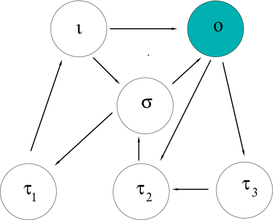
(a) $f_{\tau_{3},\tau_{3}}({\mathcal{I}}_{0})=0$

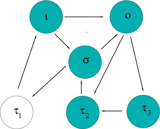
(b) $f_{\tau_{1},\tau_{1}}({\mathcal{I}}_{0})=0$

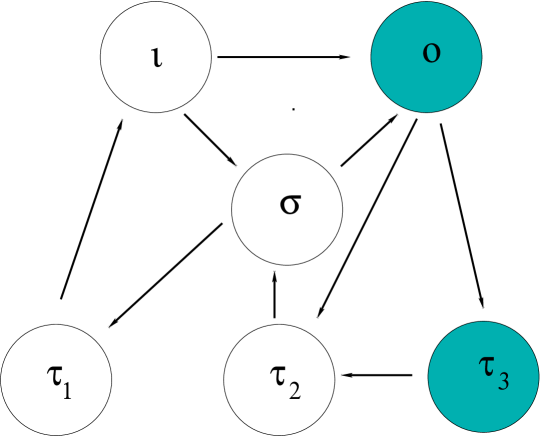
(c) $f_{\tau_{2},\tau_{2}}({\mathcal{I}}_{0})=0$

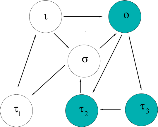
(d) $(f_{\sigma,\iota}f_{o,\sigma}-f_{\sigma,\sigma}f_{o,\iota})({\mathcal{I}}_{0})=0$

Figure 2: The four infinitesimal homeostasis patterns of (1.1). Cyan nodes are homeostatic.

The admissible system of parametrized equations for the network in Figure 1, in coordinates $X=(\iota,\sigma,\tau_{1},\tau_{2},\tau_{3},o)$, is:

$$\begin{array}[]{ccl}\dot{\iota}&=&f_{\iota}(\iota,\tau_{1},{\mathcal{I}})\\ \dot{\sigma}&=&f_{\sigma}(\iota,\sigma,\tau_{2})\\ \dot{\tau}_{1}&=&f_{\tau_{1}}(\sigma,\tau_{1})\\ \dot{\tau}_{2}&=&f_{\tau_{2}}(\tau_{2},\tau_{3},o)\\ \dot{\tau}_{3}&=&f_{\tau_{3}}(\tau_{3},o)\\ \dot{o}&=&f_{o}(\iota,\sigma,o)\end{array}$$ (1.1)

The homeostasis matrix $H$ is obtained from the Jacobian matrix $J$ of (1.1) by removing the first row and the last column (see subsection 1.1, eq. (1.9)). This leads to:

$$H=\left[\begin{array}[]{cccccccccccc|ccc}f_{\sigma,\iota}&f_{\sigma,\sigma}&0&f_{\sigma,\tau_{2}}&0\\ 0&f_{\tau_{1},\sigma}&f_{\tau_{1},\tau_{1}}&0&0&\\ 0&0&0&f_{\tau_{2},\tau_{2}}&f_{\tau_{2},\tau_{3}}\\ 0&0&0&0&f_{\tau_{3},\tau_{3}}\\ f_{o,\iota}&f_{o,\sigma}&0&0&0\end{array}\right]$$

Using row and column expansion it is straightforward to calculate

$$\det(H)=f_{\tau_{3},\tau_{3}}\,f_{\tau_{1},\tau_{1}}\,f_{\tau_{2},\tau_{2}}\,(f_{\sigma,\iota}f_{o,\sigma}-f_{\sigma,\sigma}f_{o,\iota})$$ (1.2)

The ‘determinant formula’ from [16] says that the input-output function $x_{o}({\mathcal{I}})$ undergoes infinitesimal homeostasis at ${\mathcal{I}}_{0}$ if and only if $\det(H)=0$, evaluated at $(X({\mathcal{I}}_{0}),{\mathcal{I}}_{0})$. Here $X({\mathcal{I}}_{0})$ is the equilibria used to construct the input-output function (see subsection 1.1, Lemma 1.4). The expression $\det(H)$ is a multivariate polynomial in the partial derivatives $f_{j,\ell}$ of the components of the admissible vector field. As a polynomial, $\det(H)$ is reducible with $4$ irreducible factors, so $\det(H)=0$ if and only if one of its irreducible factors vanishes.

According to [16] these irreducible factors determine the homeostasis types (see subsection 1.1, Theorem 1.5). Hence, (1.1) has $4$ homeostasis types. One of the main results of this paper says that each homeostasis type determines a unique homeostasis pattern (see Theorem 7.3). Moreover, our theory gives a purely combinatorial procedure to find the set of nodes that belong to each homeostasis pattern. When applied to Figure 1 it yields the four patterns in Figure 2.

In a simple example such as Figure 1 it is also possible to find the sets of nodes in each homeostasis pattern by a ‘bare hands’ calculation based on the admissible ODEs (see subsection 1.3). Here this calculation serves as a check on the results. Direct calculations with the ODEs can, of course, be used instead of the combinatorial approach in sufficiently simple cases.

The rest of this introduction divides into subsections. In subsection 1.1 we define the admissible differential equations that are associated to input-output networks and infinitesimal homeostasis. In subsection 1.2 we define homeostasis types and homeostasis patterns. In subsection 1.3 we determine the homeostasis patterns of the network shown in Figure 1.

1.1 Input-Output Networks and Infinitesimal Homeostasis Types

We begin by introducing the basic objects: input-output networks, network admissible differential equations, and infinitesimal homeostasis types. Our exposition follows [16].

Definition 1.2 ([16, Section 1.2]).

An input-output network is a directed graph ${\mathcal{G}}$ with nodes $\kappa\in{\mathcal{C}}$, arrows in ${\mathcal{E}}$ connecting nodes in ${\mathcal{C}}$, a distinguished input node $\iota$, and a distinguished output node $o$. The network ${\mathcal{G}}$ is a core network if every node in ${\mathcal{G}}$ is downstream from $\iota$ and upstream from $o$. $\Diamond$

An admissible system of differential equations associated with ${\mathcal{G}}$ has the form

$$\begin{split}\dot{x}_{\iota}&=f_{\iota}(x_{\iota},x_{\kappa},x_{o},{\mathcal{I}})\\ \dot{x}_{\kappa}&=f_{\kappa}(x_{\iota},x_{\kappa},x_{o})\\ \dot{x}_{o}&=f_{o}(x_{\iota},x_{\kappa},x_{o})\end{split}$$ (1.3)

where ${\mathcal{I}}\in{\mathbf{R}}$ is the input parameter, $X=(x_{\iota},x_{\kappa},x_{o})\in{\mathbf{R}}\times{\mathbf{R}}^{n}\times{\mathbf{R}}$ is the vector of state variables associated to nodes in ${\mathcal{C}}$, and $f(X,{\mathcal{I}})=(f_{\iota}(X,{\mathcal{I}}),f_{\kappa}(X),f_{o}(X))$ is a smooth family of mappings on the state space ${\mathbf{R}}\times{\mathbf{R}}^{n}\times{\mathbf{R}}$. Note that ${\mathcal{I}}$ appears only in the first equation of (1.3).

We can write (1.3) as

$$\dot{X}=f(X,{\mathcal{I}}).$$

We denote the partial derivative of the function associated to node $j$ with respect to the state variable associated to node $\ell$ by

$$f_{j,\ell}=\frac{\partial}{\partial x_{\ell}}f_{j}$$

We assume $f_{j,\ell}\equiv 0$ precisely when no arrow connects node $\ell$ to node $j$. That is, $f_{j}$ is independent of $x_{\ell}$ when there is no arrow $\ell\to j$. This is a modeling assumption made in ${\mathcal{G}}$.

Suppose $\dot{X}=f(X,{\mathcal{I}}_{0})$ has a hyperbolic equilibrium at $X_{0}$. Then the implicit function theorem implies that there is a unique family of equilibria $X({\mathcal{I}})=(x_{\iota}({\mathcal{I}}),x_{\kappa}({\mathcal{I}}),x_{o}({\mathcal{I}}))$ such that $X({\mathcal{I}}_{0})=X_{0}$ and $f(X({\mathcal{I}}),{\mathcal{I}})=0$ for all ${\mathcal{I}}$ near ${\mathcal{I}}_{0}$.

Definition 1.3.

The mapping ${\mathcal{I}}\mapsto x_{o}({\mathcal{I}})$ is an input-output function, which is defined on a neighborhood of ${\mathcal{I}}_{0}$. Infinitesimal homeostasis occurs at ${\mathcal{I}}_{0}$ if $x_{o}^{\prime}({\mathcal{I}}_{0})=0$ where ^′ indicates differentiation with respect to ${\mathcal{I}}$.

1. If $x_{o}^{\prime}({\mathcal{I}}_{0})=0$ and $x_{o}^{\prime\prime}({\mathcal{I}}_{0})\neq 0$, then $o$ has a simple homeostasis point at $(X_{0},{\mathcal{I}}_{0})$.

2. If $x_{o}^{\prime}({\mathcal{I}}_{0})=x_{o}^{\prime\prime}({\mathcal{I}}_{0})=0$ and $x_{o}^{\prime\prime\prime}({\mathcal{I}}_{0})\neq 0$, then $o$ has a chair point at $(X_{0},{\mathcal{I}}_{0})$. $\Diamond$

Nijhout et al. [14] associated homeostasis with chairs, defined as a curve that is monotone except for a flat section. The infinitesimal notion of a ‘chair point’ was introduced in [10].

1.2 Homeostasis Type and Homeostasis Pattern

Wang et al. [16] show that infinitesimal homeostasis occurs when the determinant of the homeostasis matrix $H$ is $0$, where the $(n+1)\times(n+1)$ matrix $H$ is obtained from the $(n+2)\times(n+2)$ Jacobian matrix $J$ of (1.3) by deleting its first row and last column. Indeed

$$J=\left[\begin{array}[]{rrrrrrrrrrrrrrrrrr}f_{\iota,\iota}&f_{\iota,\kappa}&f_{\iota,o}\\ f_{\kappa,\iota}&f_{\kappa,\kappa}&f_{\kappa,o}\\ f_{o,\iota}&f_{o,\kappa}&f_{o,o}\end{array}\right]\qquad\Longrightarrow\qquad H=\left[\begin{array}[]{rrrrrrrrrrrrrrrrrr}f_{\kappa,\iota}&f_{\kappa,\kappa}\\ f_{o,\iota}&f_{o,\kappa}\end{array}\right]$$ (1.9)

where $J$ and $H$ are both functions of $(X({\mathcal{I}}),{\mathcal{I}})$ as in (1.3). More precisely:

Lemma 1.4 ([16, Lemma 1.5]).

The input-output function $x_{o}({\mathcal{I}})$ undergoes infinitesimal homeostasis at ${\mathcal{I}}_{0}$ if and only if $\det(H)=0$, evaluated at $(X_{0},{\mathcal{I}}_{0})$.

In [16] the authors show that the determination of infinitesimal homeostasis in an input-output networks reduces to the study of core networks. We assume throughout that the input-output networks are core networks. See Definition 1.2.

Theorem 1.5 ([16, Theorem 1.11]).

Assume (1.3) has a hyperbolic equilibrium at $(X_{0},{\mathcal{I}}_{0})$. Then there are permutation matrices $P$ and $Q$ such that $PHQ$ is block upper triangular with square diagonal blocks $B_{1},\ldots,B_{m}$. The blocks $B_{j}$ are irreducible in the sense that each $B_{j}$ cannot be further block triangularized. It follows that

$$\det(H)=\det(B_{1})\cdots\det(B_{m})$$ (1.10)

is an irreducible factorization of $\det(H)$.

Definition 1.6.

Let $\mathcal{G}$ be an input-output network and $H$ its homeostasis matrix. Each irreducible square block $B_{\eta}$ in (1.10) is called a homeostasis block. Further we say that infinitesimal homeostasis in ${\mathcal{G}}$ is of homeostasis type $B_{\eta}$ if for all $\xi\neq\eta$

$$\det(B_{\eta})=0\ \text{ and }\ \det(B_{\xi})\neq 0.$$ (1.11)

Remark 1.7 ([16, Section 1.10]).

Let $B_{\eta}$ be a homeostasis type and let

$$h_{\eta}({\mathcal{I}})\equiv\det B_{\eta}(X({\mathcal{I}}),{\mathcal{I}})$$

A chair point of type $\eta$ occurs at ${\mathcal{I}}_{0}$ if $h_{\eta}({\mathcal{I}}_{0})=h_{\eta}^{\prime}({\mathcal{I}}_{0})=0$ and $h_{\eta}^{\prime\prime}({\mathcal{I}}_{0})\neq 0$. $\Diamond$

In principle every homeostasis type can lead to infinitesimal homeostasis, that is, $h_{\eta}({\mathcal{I}}_{0})=0$ for some input value ${\mathcal{I}}_{0}$. For simplicity, we say that node $x_{o}$ is homeostatic at ${\mathcal{I}}_{0}$. We ask: If the output node is homeostatic at ${\mathcal{I}}_{0}$, which other nodes must also be homeostatic at ${\mathcal{I}}_{0}$? Based on this question we introduce the following concept:

Definition 1.8.

A homeostasis pattern corresponding to the homeostasis block $B_{\eta}$ at ${\mathcal{I}}_{0}$ is the collection of all nodes, including the output node $o$, that are simultaneously forced to be homeostatic at $\mathcal{I}_{0}$. $\Diamond$

1.3 Example of Direct Calculation of Homeostasis Patterns

Finally, we determine the four homeostasis patterns by direct calculation. We do this by assuming that there is a one-parameter family of stable equilibria $X({\mathcal{I}})$ where $X({\mathcal{I}}_{0})=X_{0}$ using implicit differentiation with respect to ${\mathcal{I}}$ (indicated by ^′), and expanding (1.1) to first order at ${\mathcal{I}}_{0}$. The linearized system of equations is

$$\begin{array}[]{rcl}0&=&f_{\iota,\iota}\iota^{\prime}+f_{\iota,\tau_{1}}\tau_{1}^{\prime}+f_{\iota,{\mathcal{I}}}\\ 0&=&f_{\sigma,\iota}\iota^{\prime}+f_{\sigma,\sigma}\sigma^{\prime}+f_{\sigma,\tau_{2}}\tau_{2}^{\prime}\\ 0&=&f_{\tau_{1},\sigma}\sigma^{\prime}+f_{\tau_{1},\tau_{1}}\tau_{1}^{\prime}\\ 0&=&f_{\tau_{2},\tau_{2}}\tau_{2}^{\prime}+f_{\tau_{2},\tau_{3}}\tau_{3}^{\prime}\\ 0&=&f_{\tau_{3},\tau_{3}}\tau_{3}^{\prime}\\ 0&=&f_{o,\iota}\iota^{\prime}+f_{o,\sigma}\sigma^{\prime}\end{array}$$ (1.12)

Next we compute the homeostasis patterns corresponding to the $4$ homeostasis types of (1.1).

(a) Homesotasis Type: $f_{\tau_{3},\tau_{3}}=0$. Homeostatic nodes: $\{o\}$

Equation (1.12) becomes

$$\begin{array}[]{rcl}0&=&f_{\iota,\iota}\iota^{\prime}+f_{\iota,\tau_{1}}\tau_{1}^{\prime}+f_{\iota,{\mathcal{I}}}\\ 0&=&f_{\sigma,\iota}\iota^{\prime}+f_{\sigma,\sigma}\sigma^{\prime}+f_{\sigma,\tau_{2}}\tau_{2}^{\prime}\\ 0&=&f_{\tau_{1},\sigma}\sigma^{\prime}+f_{\tau_{1},\tau_{1}}\tau_{1}^{\prime}\\ 0&=&f_{\tau_{2},\tau_{2}}\tau_{2}^{\prime}+f_{\tau_{2},\tau_{3}}\tau_{3}^{\prime}\\ 0&=&0\\ 0&=&f_{o,\iota}\iota^{\prime}+f_{o,\sigma}\sigma^{\prime}\end{array}$$ (1.13)

Since $f_{\tau_{2},\tau_{2}}$ and $f_{\tau_{2},\tau_{3}}$ are generically nonzero at homeostasis, the fourth equation implies that generically $\tau_{2}^{\prime}$ and $\tau_{3}^{\prime}$ are nonzero. The second and sixth equations can be rewritten as

$$\left[\begin{array}[]{cccccccccccc|ccc}f_{\sigma,\iota}&f_{\sigma,\sigma}\\ f_{o,\iota}&f_{o,\sigma}\end{array}\right]\left[\begin{array}[]{cccccccccccc|ccc}\iota^{\prime}\\ \sigma^{\prime}\end{array}\right]=-\left[\begin{array}[]{cccccccccccc|ccc}f_{\sigma,\tau_{2}}\tau_{2}^{\prime}\\ 0\end{array}\right]$$

Generically the right hand side of this matrix equation at ${\mathcal{I}}_{0}$ is nonzero; hence generically $\iota^{\prime}$ and $\sigma^{\prime}$ are also nonzero. The third equation implies that generically $\tau_{1}^{\prime}$ is nonzero. Therefore, in this case, the only homeostatic node is $o$.

(b) Homeostasis Type: $f_{\tau_{1},\tau_{1}}=0$. Homeostatic nodes: $\{\iota,\tau_{2},\tau_{3},\sigma,o\}$

In this case (1.12) becomes

$$\begin{array}[]{rcl}0&=&f_{\iota,\iota}\iota^{\prime}+f_{\iota,\tau_{1}}\tau_{1}^{\prime}+f_{\iota,{\mathcal{I}}}\\ 0&=&f_{\sigma,\iota}\iota^{\prime}+f_{\sigma,\sigma}\sigma^{\prime}+f_{\sigma,\tau_{2}}\tau_{2}^{\prime}\\ 0&=&f_{\tau_{1},\sigma}\sigma^{\prime}\\ 0&=&f_{\tau_{2},\tau_{2}}\tau_{2}^{\prime}+f_{\tau_{2},\tau_{3}}\tau_{3}^{\prime}\\ 0&=&f_{\tau_{3},\tau_{3}}\tau_{3}^{\prime}\\ 0&=&f_{o,\iota}\iota^{\prime}+f_{o,\sigma}\sigma^{\prime}\end{array}$$ (1.14)

The fifth equation implies that generically $\tau_{3}^{\prime}=0$. The fourth equation implies that generically $\tau_{2}^{\prime}=0$. The third equation implies that generically $\sigma^{\prime}=0$ and the sixth equation implies that generically $\iota^{\prime}$ is zero. It follows that the infinitesimal homeostasis pattern is $\iota^{\prime}=\tau_{2}^{\prime}=\tau_{3}^{\prime}=\sigma^{\prime}=o^{\prime}=0$.

(c) Homeostasis Type: $f_{\tau_{2},\tau_{2}}=0$. Homeostatic nodes: $\{\tau_{3},o\}$

Equation (1.12) becomes

$$\begin{array}[]{rcl}0&=&f_{\iota,\iota}\iota^{\prime}+f_{\iota,\tau_{1}}\tau_{1}^{\prime}+f_{\iota,{\mathcal{I}}}\\ 0&=&f_{\sigma,\iota}\iota^{\prime}+f_{\sigma,\sigma}\sigma^{\prime}+f_{\sigma,\tau_{2}}\tau_{2}^{\prime}\\ 0&=&f_{\tau_{1},\sigma}\sigma^{\prime}+f_{\tau_{1},\tau_{1}}\tau_{1}^{\prime}\\ 0&=&f_{\tau_{2},\tau_{3}}\tau_{3}^{\prime}\\ 0&=&f_{\tau_{3},\tau_{3}}\tau_{3}^{\prime}\\ 0&=&f_{o,\iota}\iota^{\prime}+f_{o,\sigma}\sigma^{\prime}\end{array}$$ (1.15)

The fourth or fifth equation implies that $\tau_{3}^{\prime}=0$. The first and sixth equations imply that $\iota^{\prime}$, $\sigma^{\prime}$, and $\tau_{2}^{\prime}$ are nonzero. The third equation implies that generically $\tau_{1}^{\prime}$ is nonzero. Hence the infinitesimal homeostasis pattern is $\{\tau_{3},o\}$.

(d) Homeostasis Type: $f_{\sigma,\iota}f_{o,\sigma}-f_{\sigma,\sigma}f_{o,\iota}=0$. Homeostatic nodes $\{\tau_{2},\tau_{3},o\}$.

To repeat, Equation (1.12) is

$$\begin{array}[]{rcl}0&=&f_{\iota,\iota}\iota^{\prime}+f_{\iota,\tau_{1}}\tau_{1}^{\prime}+f_{\iota,{\mathcal{I}}}\\ 0&=&f_{\sigma,\iota}\iota^{\prime}+f_{\sigma,\sigma}\sigma^{\prime}+f_{\sigma,\tau_{2}}\tau_{2}^{\prime}\\ 0&=&f_{\tau_{1},\sigma}\sigma^{\prime}+f_{\tau_{1},\tau_{1}}\tau_{1}^{\prime}\\ 0&=&f_{\tau_{2},\tau_{2}}\tau_{2}^{\prime}+f_{\tau_{2},\tau_{3}}\tau_{3}^{\prime}\\ 0&=&f_{\tau_{3},\tau_{3}}\tau_{3}^{\prime}\\ 0&=&f_{o,\iota}\iota^{\prime}+f_{o,\sigma}\sigma^{\prime}\end{array}$$ (1.16)

The fifth equation implies generically that $\tau_{3}^{\prime}=0$ and the fourth equation implies generically that $\tau_{2}^{\prime}=0$. Again, the second and sixth equations can be rewritten in matrix form as

$$\left[\begin{array}[]{cccccccccccc|ccc}f_{\sigma,\iota}&f_{\sigma,\sigma}\\ f_{o,\iota}&f_{o,\sigma}\end{array}\right]\left[\begin{array}[]{cccccccccccc|ccc}\iota^{\prime}\\ \sigma^{\prime}\end{array}\right]=-\left[\begin{array}[]{cccccccccccc|ccc}f_{\sigma,\tau_{2}}\tau_{2}^{\prime}\\ 0\end{array}\right]=0$$

Hence generically $\iota^{\prime}$ and $\sigma^{\prime}$ are nonzero. The third equation implies that $\tau_{1}$ is nonzero. Hence the homeostatic nodes are $\tau_{2},\tau_{3},o$.

The homeostasis types of (1.1) with the corresponding homeostasis patterns are summarized in Table 1.

Homeostasis Type	Homeostasis Pattern	Figure 2
$f_{\tau_{3},\tau_{3}}=0$	$\{o\}$	(a)
$f_{\tau_{1},\tau_{1}}=0$	$\{\iota,\tau_{2},\tau_{3},\sigma,o\}$	(b)
$f_{\tau_{2},\tau_{2}}=0$	$\{\tau_{3},o\}$	(c)
$f_{\sigma,\iota}f_{o,\sigma}-f_{\sigma,\sigma}f_{o,\iota}=0$	$\{\tau_{2},\tau_{3},o\}$	(d)

Table 1: Infinitesimal homeostasis patterns for admissible systems in (1.1)

In principle the homeostasis patterns can be computed in the manner shown above; but in practice this becomes very complicated. In this paper we introduce another approach based on the pattern network ${\mathcal{P}}$ associated to the input-output network ${\mathcal{G}}$. This method is both computationally and theoretically superior. See Example 2.21. Using the pattern network we can also show that each homeostasis type leads to a unique homeostasis pattern.

1.4 Structure of the Paper

Sections 2.1-2.3, introduce the terminology of input-output networks, the homeostasis pattern network ${\mathcal{P}}$, and homeostasis induction. In Section 2.4 we state four of the main theorems of this paper, Theorems 2.17, 2.18, 2.19, 2.20, which characterize homeostasis patterns combinatorially. Section 3 provides an overview of the proofs of these main results. In Section 4, we consider combinatorial characterizations of the input-output networks ${\mathcal{G}}({\mathcal{K}})$ that are obtained by repositioning the output node on a given input-output network from $o$ to $\kappa$. Sections 5 and 6 determine the structural and appendage homeostasis pattern respectively. In Section 7 we discuss properties of homeostasis induction. Specifically we show that a homeostasis pattern uniquely determines its homeostasis type. This result is a restatement of Theorem 7.3.

The paper ends in Section 8 with a brief discussion of various types of networks that support different aspects of infinitesimal homeostasis. These networks include gene regulatory networks (GRN), input-output networks with input node = output node, and higher codimension types of infinitesimal homeostasis.

2 Aspects of Input-Output Networks

In this section, we recall additional basic terminology and results on infinitesimal homeostasis in input-output networks from [16].

2.1 Homeostasis Subnetworks

Wang et al. [16, Definition 1.14] associate a homeostasis subnetwork ${\mathcal{K}}_{\eta}\subset{\mathcal{G}}$ with each homeostasis block $B_{\eta}$ and give a graph-theoretic description of each ${\mathcal{K}}_{\eta}$.

Definition 2.1 (Definition 1.15 of [16]).

Let ${\mathcal{G}}$ be a core input-output network.

1. A simple path from node $\kappa_{1}$ to node $\kappa_{2}$ in ${\mathcal{G}}$ is a directed path that starts at $\kappa_{1}$, ends at $\kappa_{2}$, and visits each node on the path exactly once. We denote the existence of a simple path from $\kappa_{1}$ to $\kappa_{2}$ by $\kappa_{1}\rightsquigarrow\kappa_{2}$. A simple cycle is a simple path whose first and last nodes are identical.

2. An $\iota o$-simple path is a simple path from the input node $\iota$ to the output node $o$.

3. A node $\sigma$ is simple if it lies on an $\iota o$-simple path. A node $\tau$ is appendage if it is not simple.

4. A simple node $\rho$ is super-simple if it lies on every $\iota o$-simple path. $\Diamond$

We typically use $\sigma$ to denote a simple node, $\rho$ to denote a super-simple node, and $\tau$ to denote an appendage node when the type of the node is assumed a priori. Otherwise, we use $\kappa$ to denote an arbitrary node. Note that $\iota$ and $o$ are super-simple nodes.

Let $\rho_{0},\rho_{1},\ldots,\rho_{q},\rho_{q+1}$ be the super-simple nodes, where $\rho_{0}=\iota$ and $\rho_{q+1}=o$. The super-simple nodes are totally ordered by the order of their appearance on any $\iota o$-simple path, and this ordering is independent of the $\iota o$-simple path. We denote an $\iota o$-simple path by

$$\iota\rightsquigarrow\rho_{1}\rightsquigarrow\cdots\rightsquigarrow\rho_{q}\rightsquigarrow o$$

where $\rho_{j}\rightsquigarrow\rho_{j+1}$ indicates a simple path from $\rho_{j}$ to $\rho_{j+1}$. The ordering of the super-simple nodes is denoted by

$$\rho_{0}\prec\rho_{1}\prec\cdots\prec\rho_{q}\prec\rho_{q+1},$$

and $\prec$ is a total ordering. The ordering $\prec$ extends to a partial ordering of simple nodes, as follows. If there exists a super-simple node $\rho$ and an $\iota o$-simple path such that

$$\iota\rightsquigarrow\sigma_{1}\rightsquigarrow\rho\rightsquigarrow\sigma_{2}\rightsquigarrow o$$

then the partial orderings

$$\sigma_{1}\prec\rho\qquad\rho\prec\sigma_{2}\qquad\sigma_{1}\prec\sigma_{2}$$

are valid. In this partial ordering every simple node is comparable to every super-simple node but two simple nodes that lie between the same adjacent super-simple nodes need not be comparable.

We recall the definition of transitive (or strong) components of a network. Two nodes are equivalent if there is a path from one to the other and back. A transitive component is an equivalence class for this equivalence relation.

Definition 2.2.

1. Let $S$ be an $\iota o$-simple path. The complementary subnetwork of $S$ is the network $C_{S}$ whose nodes are nodes that are not in $S$ and whose arrows are those that connect nodes in $C_{S}$.

2. An appendage node $\tau$ is super-appendage if for each $C_{S}$ containing $\tau$, the transitive component of $\tau$ in $C_{S}$ consists only of appendage nodes. $\Diamond$

Note that this definition of super-appendage leads to a slightly different, but equivalent, definition of homeostasis subnetwork to the one given in [16]. However, this change enables us to define pattern networks in a more straightforward way (see Remark 2.6).

Now we start with the definition of structural subnetworks.

Definition 2.3.

Let $1\leq j\leq q+1$ and $\rho_{j-1}\prec\rho_{j}$ be two consecutive super-simple nodes. Then the $j^{th}$ simple subnetwork ${\mathcal{L}}_{j}^{\prime\prime}$, the $j^{th}$ augmented simple subnetwork ${\mathcal{L}}_{j}^{\prime}$, and the $j^{th}$ structural subnetwork ${\mathcal{L}}_{j}$ are defined in four steps as follows.

1. The $j^{th}$ simple subnetwork ${\mathcal{L}}_{j}^{\prime\prime}$ consists of simple nodes $\sigma$ where

   $$\rho_{j-1}\prec\sigma\prec\rho_{j}$$

   and all arrows connecting these nodes. Note that ${\mathcal{L}}_{j}^{\prime\prime}$ does not contain the super-simple nodes $\rho_{j-1}$ and $\rho_{j}$, and ${\mathcal{L}}_{j}^{\prime\prime}$ can be the empty set.

2. An appendage but not super-appendage node $\tau$ is linked to ${\mathcal{L}}_{j}^{\prime\prime}$ if for some complementary subnetwork $C_{S}$ the transitive component of $\tau$ in $C_{S}$ is the union of $\tau$, nodes in ${\mathcal{L}}_{j}^{\prime\prime}$, and non-super-appendage nodes. The set of $j^{th}$-linked appendage nodes $T_{j}$ is the set of non-super-appendage nodes that are linked to ${\mathcal{L}}_{j}^{\prime\prime}$.

3. The $j^{th}$ augmented simple subnetwork ${\mathcal{L}}_{j}^{\prime}$ is

   $${\mathcal{L}}_{j}^{\prime}={\mathcal{L}}_{j}^{\prime\prime}\cup T_{j}$$

   and all arrows connecting these nodes.

4. The $j^{th}$ structural subnetwork ${\mathcal{L}}_{j}$ consists of the augmented simple subnetwork $\widetilde{{\mathcal{L}}}_{j}$ and adjacent super-simple nodes. That is

   $${\mathcal{L}}_{j}=\{\rho_{j-1}\}\cup{\mathcal{L}}_{j}^{\prime}\cup\{\rho_{j}\}$$

   and all arrows connecting these nodes. $\Diamond$

Definition 2.4.

Define $\sigma_{1}\preceq\sigma_{2}$ if either $\sigma_{1}\prec\sigma_{2}$, $\sigma_{1}=\sigma_{2}$ is a super-simple node, or $\sigma_{1}$ and $\sigma_{2}$ are in the same simple subnetwork. $\Diamond$

Next we define the appendage subnetworks, which were defined in Section 1.7.2 of [16] as any transitive component of the subnetwork consisting only of appendage nodes and the arrows between them.

Definition 2.5.

An appendage subnetwork ${\mathcal{A}}$ is a transitive component of the subnetwork of super-appendage nodes. $\Diamond$

Remark 2.6.

Wang et al. [16] define an appendage subnetwork as a transitive component of appendage nodes ${\mathcal{A}}$ that satisfy the ‘no cycle’ condition. This condition is formulated in terms of the non-existence of a cycle between appendage nodes in ${\mathcal{A}}$ and the simple nodes in $C_{S}$ for all simple $\iota o$-simple paths $S$. Here, we define an appendage subnetwork as a transitive component of super-appendage nodes, which are defined in terms of transitive components with respect to $C_{S}$ for all simple $\iota o$-simple paths $S$. These two definitions are equivalent because two nodes belong to the same transitive component if and only if both nodes lie on a (simple) cycle. $\Diamond$

Wang et al. [16] show that each homeostasis subnetwork of ${\mathcal{G}}$ is either structural (satisfies Definition 2.3(d)) or appendage (satisfies Definition 2.5).

2.2 Homeostasis Pattern Network

In this subsection we construct the homeostasis pattern network ${\mathcal{P}}$ associated with ${\mathcal{G}}$ (see Definition 2.12), which serves to organize the homeostasis subnetworks and to clarify how each homeostasis subnetwork connects to the others.

The homeostasis pattern network is defined in the following steps. First, we define the structural pattern network ${\mathcal{P}}_{\mathcal{S}}$ in terms of the structural subnetworks of ${\mathcal{G}}$. Second, we define the appendage pattern network ${\mathcal{P}}_{\mathcal{A}}$ in terms of the appendage subnetworks of ${\mathcal{G}}$. Finally, we define how the nodes in ${\mathcal{P}}_{\mathcal{S}}$ connect to nodes in ${\mathcal{P}}_{\mathcal{A}}$ and conversely.

Definition 2.7.

The structural pattern network ${\mathcal{P}}_{\mathcal{S}}$ is the feedforward network whose nodes are the super-simple nodes $\rho_{j}$ and the backbone nodes $\widetilde{{\mathcal{L}}}_{j}$, where $\widetilde{{\mathcal{L}}}_{j}$ is the augmented structural subnetwork ${\mathcal{L}}_{j}^{\prime}$ treated as a single node. The nodes and arrows of ${\mathcal{P}}_{\mathcal{S}}$ are given as follows.

$$\iota=\rho_{0}\to\widetilde{{\mathcal{L}}}_{1}\to\rho_{1}\to\widetilde{{\mathcal{L}}}_{2}\to\cdots\to\widetilde{{\mathcal{L}}}_{q+1}\to\rho_{q+1}=o$$ (2.1)

If a structural subnetwork ${{\mathcal{L}}}$ consists of an arrow between two adjacent super-simple nodes (Haldane homeostasis type) then the corresponding augmented structural subnetwork ${{\mathcal{L}}^{\prime}}$ is the empty network; nevertheless the corresponding backbone node $\widetilde{{\mathcal{L}}}$ must be included in the structural pattern network ${\mathcal{P}}_{\mathcal{S}}$.

Definition 2.8.

The appendage pattern network ${\mathcal{P}}_{\mathcal{A}}$ is the network whose nodes are the components $\widetilde{{\mathcal{A}}}$ in the condensation of the subnetwork of super-appendage nodes. Such a node $\widetilde{{\mathcal{A}}}$ is called an appendage component. An arrow connects nodes $\widetilde{{\mathcal{A}}}_{1}$ and $\widetilde{{\mathcal{A}}}_{2}$ if and only if there are super-appendage nodes $\tau_{1}\in\widetilde{{\mathcal{A}}}_{1}$ and $\tau_{2}\in\widetilde{{\mathcal{A}}}_{2}$ such that $\tau_{1}\to\tau_{2}$ in ${\mathcal{G}}$. $\Diamond$

To complete the homeostasis pattern network, we describe how the nodes in ${\mathcal{P}}_{\mathcal{A}}$ and the nodes in ${\mathcal{P}}_{\mathcal{S}}$ are connected. To do so, we take advantage of the feedforward ordering of the nodes in ${\mathcal{P}}_{\mathcal{S}}$ and the feedback ordering of the nodes in ${\mathcal{P}}_{\mathcal{A}}$.

Definition 2.9.

A simple path from $\kappa_{1}$ to $\kappa_{2}$ is an appendage path if some node on this path is an appendage node and every node on this path, except perhaps for $\kappa_{1}$ and $\kappa_{2}$, is an appendage node. $\Diamond$

How ${\mathcal{P}}_{\mathcal{A}}$ connects to ${\mathcal{P}}_{\mathcal{S}}$.

Definition 2.10.

Given a node $\widetilde{{\mathcal{A}}}\in{\mathcal{P}}_{\mathcal{A}}$, we construct a unique arrow from $\widetilde{{\mathcal{A}}}$ to the structural pattern network ${\mathcal{P}}_{\mathcal{S}}$ in two steps:

1. Consider the collection of nodes ${\mathcal{V}}$ in ${\mathcal{P}}_{\mathcal{S}}$ for which there exists a simple node $\sigma\in{\mathcal{V}}$ and appendage node $\tau\in\widetilde{{\mathcal{A}}}$, such that there is an appendage path from $\tau$ to $\sigma$.

2. Let ${\mathcal{V}}_{max}(\widetilde{{\mathcal{A}}})$ be a maximal node in this collection, that is, the most downstream in ${\mathcal{P}}_{\mathcal{S}}$. It follows from (2.1) that ${\mathcal{V}}_{max}$ is either a super-simple node $\rho_{j}$ or a backbone node $\widetilde{{\mathcal{L}}}_{j}$. Maximality implies that ${\mathcal{V}}_{max}$ is uniquely defined. We then say that there is an arrow from $\widetilde{{\mathcal{A}}}$ to ${\mathcal{V}}_{max}\in{\mathcal{P}}_{\mathcal{S}}$. $\Diamond$

How ${\mathcal{P}}_{\mathcal{A}}$ is connected from ${\mathcal{P}}_{\mathcal{S}}$.

Definition 2.11.

Given a node $\widetilde{{\mathcal{A}}}\in{\mathcal{P}}_{\mathcal{A}}$ we choose uniquely an arrow from the structural pattern network ${\mathcal{P}}_{\mathcal{S}}$ to $\widetilde{{\mathcal{A}}}$ in two steps:

1. Consider the collection of nodes ${\mathcal{V}}$ in ${\mathcal{P}}_{\mathcal{S}}$ for which there exists a simple node $\sigma\in{\mathcal{V}}$ and appendage node $\tau\in\widetilde{{\mathcal{A}}}$, such that there is an appendage path from $\sigma$ to $\tau$.

2. Let ${\mathcal{V}}_{min}(\widetilde{{\mathcal{A}}})$ be a minimal node in this collection, that is, the most upstream node in ${\mathcal{P}}_{\mathcal{S}}$. Then ${\mathcal{V}}_{min}$ is either a super-simple node $\rho_{j}$ or a backbone node $\widetilde{{\mathcal{L}}}_{j}$, and the minimality implies uniqueness of ${\mathcal{V}}_{min}$. We then say that there is an arrow from ${\mathcal{V}}_{min}\in{\mathcal{P}}_{\mathcal{S}}$ to $\widetilde{{\mathcal{A}}}$. $\Diamond$

Since we consider only core input-output networks, all appendage nodes are downstream from $\iota$ and upstream from $o$. Hence, for any node $\widetilde{{\mathcal{A}}}\in{\mathcal{P}}_{\mathcal{A}}$, there always exist nodes ${\mathcal{V}}_{min},{\mathcal{V}}_{max}\in{\mathcal{P}}_{\mathcal{S}}$ as mentioned above.

Definition 2.12.

The homeostasis pattern network ${\mathcal{P}}$ is the network whose nodes are the union of the nodes of the structural pattern network ${\mathcal{P}}_{\mathcal{S}}$ and the appendage pattern network ${\mathcal{P}}_{\mathcal{A}}$. The arrows of ${\mathcal{P}}$ are the arrows of ${\mathcal{P}}_{\mathcal{S}}$, the arrows of ${\mathcal{P}}_{\mathcal{A}}$, and the arrows between ${\mathcal{P}}_{\mathcal{S}}$ and ${\mathcal{P}}_{\mathcal{A}}$ as described above. $\Diamond$

Remark 2.13.

Note that the super-simple nodes in ${\mathcal{P}}$ correspond to the super-simple nodes of ${\mathcal{G}}$. Each super-simple node $\rho_{j}\in{\mathcal{G}}$ (for $1\leq j\leq q$) belongs to exactly two structural subnetworks ${\mathcal{L}}_{j-1}$ and ${\mathcal{L}}_{j}$. Thus they are not associated to a single homeostasis subnetwork of ${\mathcal{G}}$. $\Diamond$

It follows from Remark 2.13 that there is a correspondence between the homeostasis subnetworks of ${\mathcal{G}}$ and the non-super-simple nodes of ${\mathcal{P}}$.

Remark 2.14.

1. Each structural subnetwork ${\mathcal{L}}\subseteq{\mathcal{G}}$ corresponds to the backbone node $\widetilde{{\mathcal{L}}}\in{\mathcal{P}}_{\mathcal{S}}$. Note that the augmented structural subnetworks ${\mathcal{L}}^{\prime}\subsetneq{\mathcal{L}}$ are not homeostasis subnetworks.

2. Each appendage subnetworks ${\mathcal{A}}\subset{\mathcal{G}}$ corresponds to a appendage component $\widetilde{{\mathcal{A}}}\in{\mathcal{P}}_{\mathcal{A}}$.

3. For simplicity in notation we let ${\mathcal{V}}_{\mathcal{S}}$ denote a node in ${\mathcal{P}}_{\mathcal{S}}$. Further we let $\widetilde{{\mathcal{V}}}$ denote a non-super-simple node of ${\mathcal{P}}$ and ${\mathcal{V}}$ denote its corresponding homeostasis subnetwork. $\Diamond$

2.3 Homeostasis Induction

Here we define homeostasis induction in the homeostasis pattern network ${\mathcal{P}}$, which is critical to determining the homeostasis pattern ‘triggered’ by each homeostasis subnetwork.

Definition 2.15.

Assume that the output node $o$ is homeostatic at $(X_{0},{\mathcal{I}}_{0})$, that is, $x_{o}^{\prime}({\mathcal{I}}_{0})=0$ for some input value ${\mathcal{I}}_{0}$.

1. We call the homeostasis subnetwork ${\mathcal{K}}_{\eta}$ homeostasis inducing if $h_{{\mathcal{K}}_{\eta}}\equiv\det(B_{\eta})=0$ at $(X_{0},{\mathcal{I}}_{0})$.

2. Homeostasis of a node $\kappa\in{\mathcal{G}}$ is induced by a homeostasis subnetwork ${\mathcal{K}}$, denoted ${\mathcal{K}}\Rightarrow\kappa$, if generically for $f$ in (1.3) $\kappa$ is homeostatic whenever ${\mathcal{K}}$ is homeostasis inducing.

3. A homeostasis subnetwork ${\mathcal{K}}$ induces a subset of nodes ${\mathcal{N}}$ (${\mathcal{K}}\Rightarrow{\mathcal{N}}$), if ${\mathcal{K}}\Rightarrow\kappa$ for each node $\kappa\in{\mathcal{N}}\subset{\mathcal{G}}$. $\Diamond$

By definition, every homeostasis subnetwork ${\mathcal{K}}$ induces homeostasis in the output node $o$, that is, ${\mathcal{K}}\Rightarrow o$.

Next we relate homeostatic induction between the set of homeostasis subnetworks of ${\mathcal{G}}$ to induction between nodes in the homeostasis pattern network ${\mathcal{P}}$.

Definition 2.16.

Suppose $\rho\in{\mathcal{P}}$ is a super-simple node and $\widetilde{{\mathcal{V}}}_{1},\widetilde{{\mathcal{V}}}_{2}\in{\mathcal{P}}$ are non-super-simple nodes. Let ${\mathcal{V}}_{1},{\mathcal{V}}_{2}\subset{\mathcal{G}}$ be their corresponding homeostasis subnetworks. Then $\widetilde{{\mathcal{V}}}_{1}$ induces $\widetilde{{\mathcal{V}}}_{2}$ (denoted by $\widetilde{{\mathcal{V}}}_{1}\Rightarrow\widetilde{{\mathcal{V}}}_{2}$) if and only if ${\mathcal{V}}_{1}\Rightarrow{\mathcal{V}}_{2}$. Also $\widetilde{{\mathcal{V}}}_{1}$ induces $\rho$ (denoted by $\widetilde{{\mathcal{V}}}_{1}\Rightarrow\rho$) if and only if ${\mathcal{V}}_{1}\Rightarrow\rho$. $\Diamond$

We exclude super-simple nodes of ${\mathcal{P}}$ from being ‘homeostasis inducing’ because they are not associated to a homeostasis subnetwork of ${\mathcal{G}}$ (see Remark 2.13). However, when a backbone node $\widetilde{{\mathcal{L}}}_{j}\in{\mathcal{P}}$ induces homeostasis on other nodes of ${\mathcal{P}}$, it is the corresponding structural subnetwork ${\mathcal{L}}_{j}$, with its two super-simple nodes $\rho_{j-1},\rho_{j}$ that induce homeostasis.

2.4 Characterization of Homeostasis Patterns

Now we state our main theorems, in which we use the homeostasis pattern network ${\mathcal{P}}$ to characterize homeostasis patterns.

Structural homeostasis patterns are given by the following two theorems.

Theorem 2.17 (Structural Homeostasis $\Rightarrow$ Structural Subnetworks).

A backbone node $\widetilde{{\mathcal{L}}}_{j}\in{\mathcal{P}}_{\mathcal{S}}$ induces every node of the structural pattern network ${\mathcal{P}}_{S}$ strictly downstream from $\widetilde{{\mathcal{L}}}_{j}$, but no other nodes of ${\mathcal{P}}_{S}$.

See Figure 3 for an application of Theorem 2.17.

Figure 3: An example of structural network induced by structural homeostasis. Suppose the backbone node $\widetilde{{\mathcal{L}}}_{j}$ in red is homeostasis inducing. Then Theorem 2.17 implies that the blue nodes in the structural pattern network are all homeostatic.

Theorem 2.18 (Structural Homeostasis $\Rightarrow$ Appendage Subnetworks).

A backbone node $\widetilde{{\mathcal{L}}}_{j}\in{\mathcal{P}}_{\mathcal{S}}$ induces every appendage component of ${\mathcal{P}}_{\mathcal{A}}$ whose ${\mathcal{V}}_{min}$ (see Definition 2.11) is strictly downstream, but no other nodes of ${\mathcal{P}}_{\mathcal{A}}$.

See Figure 4 for an application of Theorem 2.18.

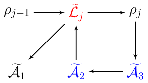
Figure 4: An example of appendage subnetworks induced by structural homeostasis. Suppose the backbone node $\widetilde{{\mathcal{L}}}_{j}$ in red is homeostasis inducing. Then by Theorem 2.18 and the fact that the super-simple node $\rho_{j}$ is strictly downstream from $\widetilde{{\mathcal{L}}}_{j}$ the blue appendage components downstream from $\rho_{j}$ are homeostatic.

The appendage homeostasis patterns are characterized by the following two theorems.

Theorem 2.19 (Appendage Homeostasis $\Rightarrow$ Structural Subnetworks).

An appendage component $\widetilde{{\mathcal{A}}}\in{\mathcal{P}}_{\mathcal{A}}$ induces every super-simple node of ${\mathcal{P}}_{S}$ downstream from ${\mathcal{V}}_{max}(\widetilde{{\mathcal{A}}})$ (see Definition 2.10), but no other super-simple nodes. Further, an appendage component $\widetilde{{\mathcal{A}}}\in{\mathcal{P}}_{\mathcal{A}}$ induces a backbone node $\widetilde{{\mathcal{L}}}_{j}$ if and only if $\widetilde{{\mathcal{L}}}_{j}$ is strictly downstream from ${\mathcal{V}}_{max}(\widetilde{{\mathcal{A}}})$.

See Figure 5 for an application of Theorem 2.17.

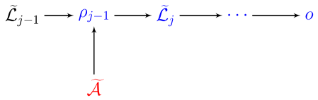
Figure 5: An example of structural subnetworks induced by appendage homeostasis. Suppose the appendage component $\widetilde{{\mathcal{A}}}$ in red is homeostasis inducing. Since $\widetilde{{\mathcal{A}}}$ connects to the super-simple node $\rho_{j-1}$, then by Theorem 2.19 the blue nodes in the structural pattern network are homeostatic.

Please recall Definitions 2.10 and 2.11 before reading the next theorem.

Theorem 2.20 (Appendage Homeostasis $\Rightarrow$ Appendage Subnetworks).

An appendage component $\widetilde{{\mathcal{A}}}_{i}\in{\mathcal{P}}_{\mathcal{A}}$ induces an appendage component $\widetilde{{\mathcal{A}}}_{j}\in{\mathcal{P}}_{\mathcal{A}}$ if and only if $\widetilde{{\mathcal{A}}}_{i}$ is strictly upstream from $\widetilde{{\mathcal{A}}}_{j}$ and every path from $\widetilde{{\mathcal{A}}}_{i}$ to $\widetilde{{\mathcal{A}}}_{j}$ in ${\mathcal{P}}$ contains a super-simple node $\rho$ satisfying ${\mathcal{V}}_{max}(\widetilde{{\mathcal{A}}}_{i})\preceq\rho\preceq{\mathcal{V}}_{min}(\widetilde{{\mathcal{A}}}_{j})$.

See Figure 6 for an application of Theorem 2.20.

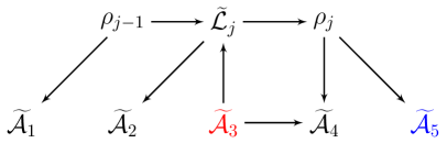
Figure 6: An example of appendage subnetworks induced by appendage homeostasis. Suppose the appendage component $\widetilde{{\mathcal{A}}}_{3}$ in red is homeostasis inducing. Since $\widetilde{{\mathcal{A}}}_{3}$ has only one path to the blue appendage component $\widetilde{{\mathcal{A}}}_{5}$ containing the super-simple node $\rho_{j}$, then by Theorem 2.20 $\widetilde{{\mathcal{A}}}_{5}$ is homeostatic, but no other appendage subnetwork is homeostatic.

Example 2.21.

We consider homeostasis patterns for the admissible systems in (1.1) obtained from Figure 1. Specifically we show how the theorems in this section lead to the determination of the homeostasis patterns that were derived by straightforward calculation from (1.12). The answer is listed in Table 1.

Case (a): $f_{\tau_{3},\tau_{3}}=0$ at ${\mathcal{I}}_{0}$: homeostasis is induced by the node $\widetilde{{\mathcal{A}}}_{3}$ of ${\mathcal{P}}_{{\mathcal{A}}}$.
Theorem 2.19 shows $\widetilde{{\mathcal{A}}}_{3}$ induces $\{o\}$, which is the only super-simple nodes of ${\mathcal{P}}_{\mathcal{S}}$ downstream from ${\mathcal{V}}_{max}(\widetilde{{\mathcal{A}}}_{3})$. And $\widetilde{{\mathcal{A}}}_{3}$ induces no backbone node. Theorem 2.20 shows $\widetilde{{\mathcal{A}}}_{3}$ induces no appendage component. Therefore, in this case the homeostasis pattern is $\{o\}$.

Case (b): $f_{\tau_{1},\tau_{1}}=0$ at ${\mathcal{I}}_{0}$: homeostasis is induced by the node $\widetilde{{\mathcal{A}}}_{1}$ of ${\mathcal{P}}_{{\mathcal{A}}}$.
Theorem 2.19 shows $\widetilde{{\mathcal{A}}}_{1}$ induces $\{\iota,o\}$, which are the super-simple nodes of ${\mathcal{P}}_{\mathcal{S}}$ downstream from ${\mathcal{V}}_{max}(\widetilde{{\mathcal{A}}}_{1})$. Also $\widetilde{{\mathcal{A}}}_{1}$ induces $\{\widetilde{{\mathcal{L}}}_{1}\}$, which is the backbone node of ${\mathcal{P}}_{\mathcal{S}}$ downstream from $\iota$. Theorem 2.20 shows $\widetilde{{\mathcal{A}}}_{1}$ induces $\{\widetilde{{\mathcal{A}}}_{2},\widetilde{{\mathcal{A}}}_{3}\}$, which are the nodes of ${\mathcal{P}}_{\mathcal{A}}$ downstream from $\widetilde{{\mathcal{A}}}_{1}$ and each path contains the super-simple node $o$ with ${\mathcal{V}}_{max}(\widetilde{{\mathcal{A}}}_{1})\preceq o\preceq{\mathcal{V}}_{min}(\widetilde{{\mathcal{A}}}_{2})$ or ${\mathcal{V}}_{min}(\widetilde{{\mathcal{A}}}_{3})$. Therefore, in this case the homeostasis pattern is $\{\iota,\ \sigma,\ o,\ \tau_{2},\ \tau_{3}\}$.

Case (c): $f_{\tau_{2},\tau_{2}}=0$ at ${\mathcal{I}}_{0}$: homeostasis is induced by the node $\widetilde{{\mathcal{A}}}_{2}$ of ${\mathcal{P}}_{{\mathcal{A}}}$.
Theorem 2.19 shows $\widetilde{{\mathcal{A}}}_{2}$ induces $\{o\}$, which is the super-simple nodes of ${\mathcal{P}}_{\mathcal{S}}$ downstream from ${\mathcal{V}}_{max}(\widetilde{{\mathcal{A}}}_{2})$. And $\widetilde{{\mathcal{A}}}_{2}$ induces no backbone node. Theorem 2.20 shows $\widetilde{{\mathcal{A}}}_{2}$ induces $\{\widetilde{{\mathcal{A}}}_{3}\}$, which is the node of ${\mathcal{P}}_{\mathcal{A}}$ downstream from $\widetilde{{\mathcal{A}}}_{2}$ and each path contains the super-simple node $o$ with ${\mathcal{V}}_{max}(\widetilde{{\mathcal{A}}}_{2})\preceq o\preceq{\mathcal{V}}_{min}(\widetilde{{\mathcal{A}}}_{3})$. Therefore, in this case the homeostasis pattern is $\{o,\ \tau_{3}\}$.

Case (d): $\det\begin{pmatrix}f_{\sigma,\iota}&f_{\sigma,\sigma}\\ f_{o,\iota}&f_{o,\sigma}\end{pmatrix}=0$ at ${\mathcal{I}}_{0}$: homeostasis is induced by node $\widetilde{{\mathcal{L}}}_{1}$ of ${\mathcal{P}}_{{\mathcal{S}}}$.
Theorem 2.17 shows $\widetilde{{\mathcal{L}}}_{1}$ induces $\{o\}$, which is the node of ${\mathcal{P}}_{\mathcal{S}}$ downstream from $\widetilde{{\mathcal{L}}}_{1}$. Theorem 2.18 shows $\widetilde{{\mathcal{L}}}_{1}$ induces $\{\widetilde{{\mathcal{A}}}_{2},\widetilde{{\mathcal{A}}}_{3}\}$, whose ${\mathcal{V}}_{min}$ are strictly downstream from $\widetilde{{\mathcal{L}}}_{1}$. Therefore, in this case the homeostasis pattern is $\{o,\ \tau_{2},\ \tau_{3}\}$.

Figure 7: Pattern network ${\mathcal{P}}$ obtained from $6$-node input-output network ${\mathcal{G}}$ illustrated in Figure 1.

3 Overview of Proofs of Theorems 2.17-2.20

The theorems that we characterize here give the homeostasis patterns $\widetilde{{\mathcal{V}}}_{1}\Rightarrow\widetilde{{\mathcal{V}}}_{2}$ or $\widetilde{{\mathcal{V}}}_{1}\not\Rightarrow\widetilde{{\mathcal{V}}}_{2}$ between any two nodes $\widetilde{{\mathcal{V}}}_{1},\widetilde{{\mathcal{V}}}_{2}$ in the homeostasis pattern network ${\mathcal{P}}$. Their proofs are done by transferring to the pattern network ${\mathcal{P}}$ the corresponding results on the input-output network ${\mathcal{G}}$. These proofs are achieved in three steps.

The first step solves the following. Given a node $\kappa\in{\mathcal{G}}$ and a homeostasis subnetwork ${\mathcal{K}}\subset{\mathcal{G}}$, determine whether ${\mathcal{K}}\Rightarrow\kappa$ for each of the four possibilities:

1. ${\mathcal{K}}$ structural and $\kappa$ simple,

2. ${\mathcal{K}}$ structural and $\kappa$ appendage,

3. ${\mathcal{K}}$ appendage and $\kappa$ simple,

4. ${\mathcal{K}}$ appendage and $\kappa$ appendage.

In the first step the proof proceeds by fixing a node $\kappa\in{\mathcal{G}}$ and considering the input-output network ${\mathcal{G}}(\kappa)$ defined as the input-output network ${\mathcal{G}}$ with input node $\iota$ and output node $\kappa$ (see Definition 4.2).

The following result describes the role of the network ${\mathcal{G}}(\kappa)$ in showing that ${\mathcal{K}}\Rightarrow\kappa$ for some subnetwork ${\mathcal{K}}$.

Lemma 3.1.

Let ${\mathcal{K}}$ be a homeostasis subnetwork of ${\mathcal{G}}$. Then ${\mathcal{K}}$ induces $\kappa$ if and only if ${\mathcal{K}}$ is a homeostasis subnetwork of ${\mathcal{G}}(\kappa)$.

Proof.

The lemma follows by recalling Definition 2.15 of homeostasis induction and by applying Theorem 1.5 to ${\mathcal{G}}(\kappa)$. ∎

The proofs of statements (1) - (4) above reduce to purely combinatorial statements. Specifically given a homeostasis subnetwork ${\mathcal{K}}$ of ${\mathcal{G}}$ and a node $\kappa\in{\mathcal{G}}$, solve the following two problems.

Determine when ${\mathcal{K}}$ is a structural subnetwork of ${\mathcal{G}}(\kappa)$.

The answer is given by Lemmas 4.5 and 4.6 in Section 4.2.

Determine when ${\mathcal{K}}$ is an appendage subnetwork of ${\mathcal{G}}(\kappa)$.

The answer is given by Lemmas 4.8 - 4.12 in Section 4.3.

At this step in the proof we work directly with the input-output networks ${\mathcal{G}}$ and ${\mathcal{G}}(\kappa)$.

The second step consists of lumping together the induced/non-induced nodes $\kappa$ into the corresponding homeostasis subneworks. That is, if ${\mathcal{K}}\Rightarrow\kappa$ then ${\mathcal{K}}\Rightarrow{\mathcal{K}}^{\prime}$, where ${\mathcal{K}}\neq{\mathcal{K}}^{\prime}$ and $\kappa\in{\mathcal{K}}^{\prime}$. This is done in several propositions in Sections 5 and 6.

The third step consists of transferring the relations of induction/non-induction between homeostasis subnetworks to relations between the nodes of the homeostasis pattern network ${\mathcal{P}}$. Since ${\mathcal{P}}$ is obtained by collapsing certain subsets of nodes of ${\mathcal{G}}$, this step follows automatically from the previous step.

4 Combinatorial Characterization of IO Networks ${\mathcal{G}}(\kappa)$

4.1 The Input-Output Networks ${\mathcal{G}}(\kappa)$

Definition 4.1.

Let ${\mathcal{G}}$ be an input-output network with input node $\iota$ and output node $o$, and let $\kappa\in{\mathcal{G}}$ be a node. Define the input-output network ${\mathcal{G}}(\kappa)$ to be the network ${\mathcal{G}}$ with input node $\iota$ and output node $\kappa$. $\Diamond$

Definition 4.2.

Let ${\mathcal{G}}$ be an input-output network and let $\kappa\in{\mathcal{G}}$ be a node. Define the nodes $\sigma^{u}(\kappa)$ and $\sigma^{d}(\kappa)$ as follows.

1. If $\kappa$ is simple, then $\sigma^{u}(\kappa)=\kappa=\sigma^{d}(\kappa)$.

2. If $\kappa$ is appendage, then $\sigma^{u}(\kappa)$ is a minimal upstream simple node with an appendage path to $\kappa$ and $\sigma^{d}(\kappa)$ is a maximal downstream simple node with an appendage path from $\kappa$. $\Diamond$

Remark 4.3.

Let ${\mathcal{A}}$ be an appendage subnetwork. Since ${\mathcal{A}}$ is a transitive component, we can choose an arbitrary node $\tau\in{\mathcal{A}}$ and observe that $\sigma^{u}({\mathcal{A}})=\sigma^{u}(\tau)$ and $\sigma^{d}({\mathcal{A}})=\sigma^{d}(\tau)$. $\Diamond$

If $\kappa$ is an appendage node, then $\sigma^{u}(\kappa)$ is upstream from $\kappa$ and $\sigma^{d}(\kappa)$ is downstream from $\kappa$. If $\kappa$ is a node in an appendage subnetwork ${\mathcal{A}}$, then $\sigma^{u}(\kappa)$ is contained in some structural subnetwork or is a super-simple node ${\mathcal{V}}$ with an arrow $\widetilde{{\mathcal{V}}}\to\widetilde{{\mathcal{A}}}$ and $\sigma^{d}(\kappa)$ is contained in some structural subnetwork or is a super-simple node ${\mathcal{V}}$ with an arrow $\widetilde{{\mathcal{A}}}\to\widetilde{{\mathcal{V}}}$.

Lemma 4.4.

An appendage node $\tau$ is in the $j^{th}$ linked appendage subnetwork $T_{j}$ if and only if there is a simple cycle $C$ that contains $\tau$ and a node in the simple subnetwork ${\mathcal{L}}_{j}^{\prime\prime}$, but $C$ does not contain any super-simple node.

Proof.

Recall that $\tau\in T_{j}$ if, for some complementary subnetwork $C_{S}$, the transitive component of $\tau$ in $C_{S}$ is the union of $\tau$, nodes in ${\mathcal{L}}^{\prime}_{j}$, and non-super-appendage nodes. The statement then follows because two nodes belong to the same transitive component if and only if some cycle includes them. ∎

4.2 Structural Subnetworks of ${\mathcal{G}}(\kappa)$

We start with a lemma that characterizes the super-simple nodes of ${\mathcal{G}}$ that are super-simple nodes of ${\mathcal{G}}(\kappa)$:

Lemma 4.5.

Let $\rho$ be a super-simple node of ${\mathcal{G}}$ and let $\kappa$ be a node in ${\mathcal{G}}$. Then $\rho$ is a super-simple node of ${\mathcal{G}}(\kappa)$ if and only if $\rho\preceq\sigma^{u}(\kappa)$.

Proof.

$(\Longleftarrow)$ Suppose $\rho\preceq\sigma^{u}(\kappa)$. Consider a simple path $p=\iota\rightsquigarrow\kappa$. Let $\sigma^{\prime}$ be the last simple node on this path. We show that $\rho$ is super-simple in two parts. If $\kappa$ is a simple node, then $\sigma^{u}(\kappa)=\kappa$ and $\sigma^{\prime}=\kappa$ because it is the last simple node in $p$. Then $\rho\preceq\sigma^{\prime}$ and $p$ contains $\rho$. If $\kappa$ is an appendage node, then $\rho\preceq\sigma^{\prime}$ since $\sigma^{u}(\kappa)$ is minimal. Consequently, $p$ contains $\rho$. Since the simple path from $\iota$ to $\kappa$ was arbitrary, $\rho$ is super-simple in ${\mathcal{G}}(\kappa)$.

$(\Longrightarrow)$ Suppose $\sigma^{u}(\kappa)\prec\rho$. Then there is a simple path $\iota\rightsquigarrow\sigma^{u}(\kappa)$ which avoids $\rho$. If $\sigma^{u}(\kappa)\neq\kappa$, there is an appendage path $\sigma^{u}(\kappa)\rightsquigarrow\kappa$, which by definition avoids $\rho$. There is a simple path $\iota\rightsquigarrow\sigma^{u}(\kappa)$ which avoid $\rho$ since $\sigma^{u}(\kappa)\prec\rho$. The concatenation of these paths, $\iota\rightsquigarrow\sigma^{u}(\kappa)\rightsquigarrow\kappa$, avoids $\rho$ and shows $\rho$ is not super-simple in ${\mathcal{G}}(\kappa)$. If $\sigma^{u}(\kappa)=\kappa$, then the simple path $\iota\rightsquigarrow\sigma^{u}(\kappa)$ shows $\rho$ is not super-simple in ${\mathcal{G}}(\kappa)$. ∎

The next result shows that a structural subnetwork of ${\mathcal{G}}$ is a structural subnetwork of ${\mathcal{G}}(\kappa)$ when its two super-simple nodes are super-simple nodes of ${\mathcal{G}}(\kappa)$.

Lemma 4.6.

Let $\kappa\in{\mathcal{G}}$ be a node and let ${\mathcal{L}}_{j}$ be the $j^{th}$ structural subnetwork of ${\mathcal{G}}$. Suppose $\rho_{j-1},\,\rho_{j}\in{\mathcal{L}}_{j}$ are adjacent super-simple nodes of ${\mathcal{G}}(\kappa)$. Then ${\mathcal{L}}_{j}$ is a structural subnetwork of ${\mathcal{G}}(\kappa)$.

Proof.

Let ${\mathcal{L}}_{j}(\kappa)$ be the structural subnetwork of ${\mathcal{G}}(\kappa)$ that has super-simple nodes $\rho_{j-1}$ and $\rho_{j}$. Since $\rho_{j-1}$ and $\rho_{j}$ are adjacent super-simple nodes of both ${\mathcal{G}}$ and ${\mathcal{G}}(\kappa)$, the simple networks ${\mathcal{L}}_{j}^{\prime\prime}$ and ${\mathcal{L}}_{j}^{\prime\prime}(\kappa)$ are equal. We need to show that the linked appendage nodes $T_{j}$ and $T_{j}(\kappa)$ are equal.

Suppose there exists $\tau\in T_{j}(\kappa)$ with $\tau\notin T_{j}$. By Lemma 4.4, there is a simple cycle $C$ that contains $\tau$, a node of ${\mathcal{L}}_{j}^{\prime}$, and no super-simple nodes of ${\mathcal{G}}(\kappa)$. Since $\tau\notin T_{j}$, $C$ must contain a super-simple node $\rho$ of ${\mathcal{G}}$ that is not super-simple in ${\mathcal{G}}(\kappa)$. By Lemma 4.5, this implies $\rho_{j}\prec\rho$. But $C$ also contains a simple node $\sigma\in{\mathcal{L}}_{j}^{\prime}$, so this implies there is a simple path $\iota\rightsquigarrow\sigma\rightsquigarrow\tau\rightsquigarrow\rho\rightsquigarrow o$, contradicting $\tau$ being appendage in ${\mathcal{G}}$. Therefore $\tau\in T_{j}$. Reversing the roles of $T_{j}$ and $T_{j}(\kappa)$ in the above argument shows that if $\tau\in T_{j}$ then $\tau\in T_{j}(\kappa)$, completing the proof that $T_{j}=T_{j}(\kappa)$.

Now $\rho_{j-1}$ and $\rho_{j}$ are super-simple in ${\mathcal{G}}(\kappa)$, ${\mathcal{L}}_{j}^{\prime\prime}={\mathcal{L}}_{j}^{\prime\prime}(\kappa)$, and $T_{j}=T_{j}(\kappa)$. Therefore ${\mathcal{L}}_{j}$ is a structural subnetwork of ${\mathcal{G}}(\kappa)$. ∎

Remark 4.7.

The network ${\mathcal{G}}(\kappa)$ may have other structural subnetworks, but we study the homeostasis pattern induced by homeostasis subnetworks of ${\mathcal{G}}$. Hence, we focus on whether a structural subnetwork of ${\mathcal{G}}$ is still a structural subnetwork of ${\mathcal{G}}(\kappa)$.

An appendage subnetwork ${\mathcal{A}}$ of ${\mathcal{G}}$ is not a structural subnetwork of ${\mathcal{G}}(\kappa)$, because ${\mathcal{A}}$ is transitive and thus has no super-simple nodes. $\Diamond$

4.3 Appendage Subnetworks of ${\mathcal{G}}(\kappa)$

Lemma 4.8.

Let ${\mathcal{A}}$ be an appendage subnetwork of ${\mathcal{G}}$ and let $\sigma_{1},\sigma_{2}$ be simple nodes of ${\mathcal{G}}$ with appendage paths ${\mathcal{A}}\rightsquigarrow\sigma_{1}$ and $\sigma_{2}\rightsquigarrow{\mathcal{A}}$. Then $\sigma_{1}\preceq\sigma_{2}$. Moreover, either $\sigma_{1}=\sigma_{2}$ is a super-simple node or $\sigma_{1}\prec\sigma_{2}$.

Proof.

Since $\sigma_{1},\sigma_{2}$ are simple nodes there are simple paths $\iota\rightsquigarrow\sigma_{2}$ and $\sigma_{1}\rightsquigarrow o$ that contain only simple nodes. By contradiction, suppose that $\sigma_{2}\prec\sigma_{1}$. Then $\sigma_{2}$ is not on the path $\sigma_{1}\rightsquigarrow o$ and $\sigma_{1}$ is not on the path $\iota\rightsquigarrow\sigma_{2}$. By concatenating paths we produce a simple path

$$\iota\rightsquigarrow\sigma_{2}\rightsquigarrow{\mathcal{A}}\rightsquigarrow\sigma_{1}\rightsquigarrow o,$$

which contradicts ${\mathcal{A}}$ being an appendage subnetwork.

Next we show that it is impossible for both $\sigma_{1}$ and $\sigma_{2}$ to be contained in the same simple subnetwork ${\mathcal{L}}^{\prime\prime}$. By contradiction, suppose there exists a simple subnetwork ${\mathcal{L}}^{\prime\prime}$ such that $\sigma_{1},\sigma_{2}\in{\mathcal{L}}^{\prime\prime}$. There are three possibilities.

• If there is a simple path $\iota\rightsquigarrow\sigma_{1}\rightsquigarrow\sigma_{2}\rightsquigarrow o$, then there exists a simple path

  $$\iota\rightsquigarrow\sigma_{1}\rightsquigarrow{\mathcal{A}}\rightsquigarrow\sigma_{2}\rightsquigarrow o,$$

  contradicting that ${\mathcal{A}}$ is an appendage subnetwork.

• If there is a simple path $\iota\rightsquigarrow\sigma_{2}\rightsquigarrow\sigma_{1}\rightsquigarrow o$, then the cycle

  $$\sigma_{1}\rightsquigarrow{\mathcal{A}}\rightsquigarrow\sigma_{2}\rightsquigarrow\sigma_{1}$$

  contradicts the fact that every node in ${\mathcal{A}}$ is super-appendage.

• If neither of the above paths exists, then there is a simple path $\iota\rightsquigarrow\sigma_{1}\rightsquigarrow o$ that avoids $\sigma_{2}$ and a path $\iota\rightsquigarrow\sigma_{2}\rightsquigarrow o$ that avoids $\sigma_{1}$. In this case, the path

  $$\iota\rightsquigarrow\sigma_{1}\rightsquigarrow{\mathcal{A}}\rightsquigarrow\sigma_{2}\rightsquigarrow o$$

  contradicts the fact that ${\mathcal{A}}$ is an appendage subnetwork.

We can now conclude that either $\sigma_{1}=\sigma_{2}$ is a super-simple node or $\sigma_{1}\prec\sigma_{2}$. ∎

Lemma 4.9.

Let ${\mathcal{A}}$ be an appendage subnetwork of ${\mathcal{G}}$ and let $\kappa\in{\mathcal{G}}$ be a node that is not in ${\mathcal{A}}$. If there is a path from ${\mathcal{A}}$ to $\kappa$ and every such path passes through a super-simple node $\rho$ of ${\mathcal{G}}$ satisfying $\sigma^{d}({\mathcal{A}})\preceq\rho\preceq\sigma^{u}(\kappa)$, then ${\mathcal{A}}$ is an appendage subnetwork of ${\mathcal{G}}(\kappa)$.

Proof.

First we show that the nodes of ${\mathcal{A}}$ are appendage in ${\mathcal{G}}(\kappa)$. By contradiction, suppose $\tau\in{\mathcal{A}}$ is a simple node of ${\mathcal{G}}(\kappa)$. Let $p=\iota\rightsquigarrow\tau\rightsquigarrow\kappa$ be a simple path in ${\mathcal{G}}(\kappa)$. Let $\sigma_{1}$ be the last simple node of ${\mathcal{G}}$ on the path $\iota\rightsquigarrow\tau$. Let $\sigma_{2}$ and $\rho^{\prime}$ be the first simple node and first super-simple node of ${\mathcal{G}}$ on the path $\tau\rightsquigarrow\kappa$, respectively.

If $\rho^{\prime}\preceq\sigma_{1}$ then the path $\iota\rightsquigarrow\sigma_{1}$ passes through $\rho^{\prime}$, contradicting that $p$ is a simple path. Otherwise, suppose $\sigma_{1}\prec\rho^{\prime}$. Since there are appendage paths $\sigma_{1}\rightsquigarrow{\mathcal{A}}$ and ${\mathcal{A}}\rightsquigarrow\sigma_{2}$ and $\sigma_{1}\neq\sigma_{2}$, by Lemma 4.8, $\sigma_{2}\prec\sigma_{1}$. There is therefore a super-simple node $\rho^{\prime\prime}$ of ${\mathcal{G}}$ with $\sigma_{2}\preceq\rho^{\prime\prime}\preceq\sigma_{1}$. The segments $\iota\rightsquigarrow\sigma_{1}$ and $\sigma_{2}\rightsquigarrow\rho^{\prime}$ of $p$ thus both contain $\rho^{\prime\prime}$, contradicting that $p$ is a simple path. We conclude that each node $\tau\in{\mathcal{A}}$ is an appendage node of ${\mathcal{G}}(\kappa)$.

Next we show that if there is a cycle ${\mathcal{A}}\rightsquigarrow\tau\rightsquigarrow{\mathcal{A}}$ consisting only of appendage nodes of ${\mathcal{G}}(\kappa)$, then $\tau$ is an appendage node of ${\mathcal{G}}$. Suppose not, then there exists a cycle ${\mathcal{A}}\rightsquigarrow\tau\rightsquigarrow{\mathcal{A}}$ contains a simple node of ${\mathcal{G}}$ but only appendage nodes of ${\mathcal{G}}(\kappa)$. Let $\sigma$ be the first simple node of ${\mathcal{G}}$ on the cycle, starting from ${\mathcal{A}}$. Since $\sigma$ is not a simple node of ${\mathcal{G}}(\kappa)$, by Lemma 4.5, either $\sigma\succ\sigma^{u}(\kappa)$ or $\sigma$ and $\sigma^{u}(\kappa)$ are incomparable. On the other hand, there is an appendage path from ${\mathcal{A}}$ to $\sigma$ which implies $\sigma\preceq\sigma^{d}({\mathcal{A}})$ or $\sigma$ and $\sigma^{d}({\mathcal{A}})$ are incomparable. But this implies $\sigma^{u}(\kappa)\prec\sigma^{d}({\mathcal{A}})$, which contradicts the assumption $\sigma^{d}({\mathcal{A}})\preceq\rho\preceq\sigma^{u}(\kappa)$.

Now we claim that there is no appendage subnetwork ${\mathcal{A}}^{\prime}$ of ${\mathcal{G}}(\kappa)$, such that ${\mathcal{A}}\subsetneq{\mathcal{A}}^{\prime}$. Suppose not, there exists such a appendage subnetworks ${\mathcal{A}}^{\prime}$. Then ${\mathcal{A}}^{\prime}$ is a a transitive component consisting of only appendage nodes of ${\mathcal{G}}$. Hence, ${\mathcal{A}}^{\prime}$ must be an appendage subnetwork of ${\mathcal{G}}$ containing ${\mathcal{A}}$. This contradicts ${\mathcal{A}}$ an appendage subnetwork of ${\mathcal{G}}$ that is not transitive with other appendage subnetworks.

Finally, we show that ${\mathcal{A}}$ is a transitive component of super-appendage nodes of ${\mathcal{G}}(\kappa)$; that is, ${\mathcal{A}}$ is an appendage subnetwork of ${\mathcal{G}}(\kappa)$. Suppose not, then each node $\tau\in{\mathcal{A}}$ is linked to a simple subnetwork ${\mathcal{L}}^{\prime\prime}$ of ${\mathcal{G}}(\kappa)$. By Lemma 4.4, there is a simple cycle $C$ that avoids super-simple node of ${\mathcal{G}}(\kappa)$ and contains $\tau$ as well as a simple node of ${\mathcal{G}}(\kappa)$. Since ${\mathcal{A}}$ is a transitive  component of the appendage nodes of ${\mathcal{G}}$, $C$ must contain a simple node of ${\mathcal{G}}$. But $\tau$ is not a linked appendage node of ${\mathcal{G}}$, so $C$ must contain a super-simple node $\rho^{\prime}$ of ${\mathcal{G}}$. Since $\rho^{\prime}$ is not super-simple in ${\mathcal{G}}(\kappa)$, by Lemma 4.5 $\rho\succ\sigma^{u}(\kappa)$. Let $\sigma$ be the first simple node of ${\mathcal{G}}$ on the path ${\mathcal{A}}\rightsquigarrow\rho^{\prime}$ in $C$. We have $\sigma\preceq\sigma^{d}({\mathcal{A}})$ or $\sigma$ and $\sigma^{d}({\mathcal{A}})$ are incomparable. But then the path $\sigma\rightsquigarrow\rho^{\prime}$ passes through $\rho$. Since $\rho\preceq\sigma^{u}(\kappa)$, $\rho$ is a super-simple node of ${\mathcal{G}}(\kappa)$ by Lemma 4.5, contradicting that $C$ avoids super-simple nodes of ${\mathcal{G}}(\kappa)$. We conclude that ${\mathcal{A}}$ is an appendage subnetwork of ${\mathcal{G}}(\kappa)$. ∎

Lemma 4.10.

Let ${\mathcal{A}}$ be an appendage subnetwork of ${\mathcal{G}}$ and let $\kappa$ be a node in ${\mathcal{G}}$. Suppose a cycle $C$ in ${\mathcal{G}}$ contains some node $\tau\in{\mathcal{A}}$ and some node that is not in ${\mathcal{A}}$. Suppose also that $C$ avoids super-simple nodes of ${\mathcal{G}}(\kappa)$. Then ${\mathcal{A}}$ is not an appendage subnetwork of ${\mathcal{G}}(\kappa)$.

Proof.

The cycle $C$ can take three possible forms, and we will show that ${\mathcal{A}}$ is not an appendage subnetwork of ${\mathcal{G}}(\kappa)$ in each case.

1. $C$ consists of simple nodes of ${\mathcal{G}}(\kappa)$. Since $C$ contains a node $\tau\in{\mathcal{A}}$, this immediately implies ${\mathcal{A}}$ is not an appendage subnetwork of ${\mathcal{G}}(\kappa)$.

2. $C$ consists of appendage nodes of ${\mathcal{G}}(\kappa)$. A node $\tau\in{\mathcal{A}}$ forms a cycle with appendage nodes of ${\mathcal{G}}(\kappa)$ that are not in ${\mathcal{A}}$. Consequently, ${\mathcal{A}}$ is not a transitive component of appendage nodes of ${\mathcal{G}}(\kappa)$ and therefore not an appendage subnetwork.

3. $C$ consists of both simple and appendage nodes of ${\mathcal{G}}(\kappa)$. By Lemma 4.4, any appendage node $\eta$ of ${\mathcal{G}}(\kappa)$ on $C$ is linked to the simple nodes of ${\mathcal{G}}(\kappa)$ on $C$ and hence $\eta$ is a non-super-appendage node. Therefore any node $\tau\in{\mathcal{A}}$ on $C$ is either simple or non-super-appendage in ${\mathcal{G}}(\kappa)$. We conclude that ${\mathcal{A}}$ is not an appendage subnetwork of ${\mathcal{G}}(\kappa)$. ∎

Lemma 4.11.

Let ${\mathcal{A}}$ be an appendage subnetwork of ${\mathcal{G}}$ and let $\kappa$ be a node in ${\mathcal{G}}$. If $\sigma^{u}(\kappa)\prec\sigma^{d}({\mathcal{A}})$, then ${\mathcal{A}}$ is not an appendage subnetwork of ${\mathcal{G}}(\kappa)$.

Proof.

By Lemma 4.8, $\sigma^{d}({\mathcal{A}})\preceq\sigma^{u}({\mathcal{A}})$. Then there exists a simple cycle $C={\mathcal{A}}\rightsquigarrow\sigma^{d}({\mathcal{A}})\rightsquigarrow\sigma^{u}({\mathcal{A}})\rightsquigarrow{\mathcal{A}}$ where two segments ${\mathcal{A}}\rightsquigarrow\sigma^{d}({\mathcal{A}})$ and $\sigma^{u}({\mathcal{A}})\rightsquigarrow{\mathcal{A}}$ are appendage paths while every simple node of ${\mathcal{G}}$ on $C$ is in the segment $\sigma^{d}({\mathcal{A}})\rightsquigarrow\sigma^{u}({\mathcal{A}})$.

Now we claim that $C$ does not contain a super-simple node of ${\mathcal{G}}(\kappa)$. Given the claim, Lemma 4.10 implies ${\mathcal{A}}$ is not an appendage subnetwork of $\kappa$. Thus it remains to prove the claim.

Consider any simple node $\sigma$ of ${\mathcal{G}}$ on the segment $\sigma^{d}({\mathcal{A}})\rightsquigarrow\sigma^{u}({\mathcal{A}})$ in $C$. Since $\sigma^{u}(\kappa)\prec\sigma^{d}({\mathcal{A}})$, this implies that $\sigma^{u}(\kappa)\prec\sigma$. Thus there is a simple path $\iota\rightsquigarrow\sigma^{u}(\kappa)$ that avoids every simple node of ${\mathcal{G}}$ on $C$.

If $\kappa$ is a simple node, then $\sigma^{u}(\kappa)=\kappa$. This gives an input-output path in ${\mathcal{G}}(\kappa)$ that avoids every node in $C$, verifying the claim. If $\kappa$ is an appendage node, then $\sigma^{u}(\kappa)\neq\kappa$. There is an appendage path $\sigma^{u}(\kappa)\rightsquigarrow\kappa$. For the sake of contradiction, suppose there is a node $\tau$ on $\sigma^{u}(\kappa)\rightsquigarrow\kappa$ that is also on $C$. Either $\tau$ is on the segment ${\mathcal{A}}\rightsquigarrow\sigma^{d}({\mathcal{A}})$ or the segment $\sigma^{u}({\mathcal{A}})\rightsquigarrow{\mathcal{A}}$. If $\tau$ is on ${\mathcal{A}}\rightsquigarrow\sigma^{d}({\mathcal{A}})$, then there is an appendage path $\sigma^{u}(\kappa)\rightsquigarrow\tau\rightsquigarrow\sigma^{d}({\mathcal{A}})$. Since $\sigma^{u}(\kappa)\prec\sigma^{d}({\mathcal{A}})$, this gives an input-output simple path

$$\iota\rightsquigarrow\sigma^{u}(\kappa)\rightsquigarrow\tau\rightsquigarrow\sigma^{d}({\mathcal{A}})\rightsquigarrow o$$

which contradicts that $\tau$ is appendage in ${\mathcal{G}}$. If $\tau$ is on $\sigma^{u}({\mathcal{A}})\rightsquigarrow{\mathcal{A}}$, then this gives an appendage path $\sigma^{u}(\kappa)\rightsquigarrow\tau\rightsquigarrow{\mathcal{A}}$. Since $\sigma^{u}(\kappa)\prec\sigma^{u}({\mathcal{A}})$, this contradicts that $\sigma^{u}({\mathcal{A}})$ is a minimal simple node with an appendage path to ${\mathcal{A}}$. We conclude that the appendage path $\sigma^{u}(\kappa)\rightsquigarrow\kappa$ does not contain a node of $C$. Therefore, the simple path $\iota\rightsquigarrow\sigma^{u}(\kappa)\rightsquigarrow\kappa$ is an input-output path in ${\mathcal{G}}(\kappa)$ that avoids $C$. This proves the claim. ∎

Lemma 4.12.

Let ${\mathcal{A}}$ be an appendage subnetwork of ${\mathcal{G}}$ and let $\kappa$ be a node in ${\mathcal{G}}$. If both $\sigma^{u}(\kappa)$ and $\sigma^{d}({\mathcal{A}})$ are nodes in a simple subnetwork ${\mathcal{L}}_{j}^{\prime\prime}$ of ${\mathcal{G}}$, then ${\mathcal{A}}$ is not an appendage subnetwork of ${\mathcal{G}}(\kappa)$.

Proof.

The proof proceeds by stating two claims, proving the lemma from the claims, and then proving the claims.

Claim 1: There exists a simple path $p=\rho_{j-1}\rightsquigarrow\rho_{j}$, such that $\rho_{j-1}$ is the only super-simple node of ${\mathcal{G}}(\kappa)$ on $p$.

Claim 2: The appendage path $\sigma^{u}({\mathcal{A}})\rightsquigarrow{\mathcal{A}}$ does not contain super-simple nodes of ${\mathcal{G}}(\kappa)$.

Assuming the claims, we consider the relation between $\sigma^{d}({\mathcal{A}})$ and the path $p=\rho_{j-1}\rightsquigarrow\rho_{j}$ in the first claim and split the proof into two cases as follows.

Assume $\sigma^{d}({\mathcal{A}})$ is on the path $p$.

Then there is a simple path $\sigma^{d}({\mathcal{A}})\rightsquigarrow\rho_{j}$ avoids super-simple nodes of ${\mathcal{G}}(\kappa)$. By Lemma 4.8, $\sigma^{d}({\mathcal{A}})\prec\rho_{j}\preceq\sigma^{u}({\mathcal{A}})$ so there is a simple path $\sigma^{d}({\mathcal{A}})\rightsquigarrow\sigma^{u}({\mathcal{A}})$ which avoids super-simple nodes of ${\mathcal{G}}(\kappa)$. If an appendage path ${\mathcal{A}}\rightsquigarrow\sigma^{d}({\mathcal{A}})$ contains a super-simple node of ${\mathcal{G}}(\kappa)$, then the simple path $\iota\rightsquigarrow\sigma^{d}({\mathcal{A}})\rightsquigarrow{\mathcal{A}}\rightsquigarrow\kappa$ which contains this super-simple node shows ${\mathcal{A}}$ is not an appendage subnetwork of ${\mathcal{G}}(\kappa)$. If an appendage path ${\mathcal{A}}\rightsquigarrow\sigma^{d}({\mathcal{A}})$ does not contain a super-simple node of ${\mathcal{G}}(\kappa)$ then we have found a super-simple node avoiding cycle

$$C={\mathcal{A}}\rightsquigarrow\sigma^{d}({\mathcal{A}})\rightsquigarrow\sigma^{u}({\mathcal{A}})\rightsquigarrow{\mathcal{A}},$$

and by Lemma 4.10, ${\mathcal{A}}$ is not an appendage subnetwork of ${\mathcal{G}}(\kappa)$.

Assume every path $\rho_{j-1}\rightsquigarrow\sigma^{d}({\mathcal{A}})\rightsquigarrow\rho_{j}$ contains a super-simple node of ${\mathcal{G}}(\kappa)$ other than $\rho_{j-1}$.

If there is a path $\sigma^{d}({\mathcal{A}})\rightsquigarrow\rho_{j}$ that does not contain a super-simple node of ${\mathcal{G}}(\kappa)$, then there is a simple path $\sigma^{d}({\mathcal{A}})\rightsquigarrow\sigma^{u}({\mathcal{A}})$ that avoids super-simple nodes of ${\mathcal{G}}(\kappa)$. This is the same situation deduced in case (1), so ${\mathcal{A}}$ is not an appendage subnetwork of ${\mathcal{G}}(\kappa)$. Suppose there is a path $\sigma^{d}({\mathcal{A}})\rightsquigarrow\rho_{j}$ which contains a super-simple node $\rho(\kappa)$ of ${\mathcal{G}}(\kappa)$. Since there is a path $p=\rho_{j-1}\rightsquigarrow\rho_{j}$ that avoids super-simple nodes of ${\mathcal{G}}(\kappa)$, there is a simple path

$$p_{1}=\iota\rightsquigarrow\rho_{j-1}\rightsquigarrow\sigma^{u}({\mathcal{A}})\rightsquigarrow{\mathcal{A}}\rightsquigarrow\sigma^{d}({\mathcal{A}})\rightsquigarrow\rho(\kappa).$$

Let $p_{2}=\rho(\kappa)\rightsquigarrow\kappa$ be a simple path. If $p_{1}$ and $p_{2}$ do not overlap, then the concatenation of $p_{1}$ and $p_{2}$ shows ${\mathcal{A}}$ is not an appendage subnetwork of ${\mathcal{G}}(\kappa)$. If $p_{1}$ and $p_{2}$ overlap, they overlap in an appendage node $\tau$ of ${\mathcal{G}}$. If $\tau$ is on the segment $\sigma^{u}({\mathcal{A}})\rightsquigarrow{\mathcal{A}}$, then this implies there is an appendage path from $\widetilde{{\mathcal{L}}}_{j}$ to ${\mathcal{A}}$, contradicting that $\sigma^{u}({\mathcal{A}})$ is minimal. Therefore, $\tau$ is on the segment ${\mathcal{A}}\rightsquigarrow\sigma^{d}({\mathcal{A}})$. Let $\tau$ be the first node on $p_{1}$ which is on $p_{2}$. The simple path

$$p_{1}=\iota\rightsquigarrow\rho_{j-1}\rightsquigarrow\sigma^{u}({\mathcal{A}})\rightsquigarrow{\mathcal{A}}\rightsquigarrow\tau\rightsquigarrow\kappa$$

shows that ${\mathcal{A}}$ is not an appendage subnetwork of ${\mathcal{G}}(\kappa)$.

We now proceed to prove the claims.

Proof of Claim 1: Suppose $\rho_{j-1}\preceq\sigma^{u}(\kappa)$ is the most downstream super-simple node of ${\mathcal{G}}$. Consider a path $\rho_{j-1}\rightsquigarrow\sigma^{u}(\kappa)$. From Lemma 4.5, $\rho_{j-1}$ is a super-simple node of ${\mathcal{G}}(\kappa)$. If there is no other super-simple node of ${\mathcal{G}}(\kappa)$ on this path, then we take $p$ to be the path $\rho_{j-1}\rightsquigarrow\sigma^{u}(\kappa)\rightsquigarrow\rho_{j}$. If there exists other super-simple nodes of ${\mathcal{G}}(\kappa)$ on $\rho_{j-1}\rightsquigarrow\sigma^{u}(\kappa)$, let $\sigma$ be the first super-simple node of ${\mathcal{G}}(\kappa)$ on this path. Since $\sigma$ is a simple node of ${\mathcal{G}}$, there is a path $p=\rho_{j-1}\rightsquigarrow\rho_{j}$ which avoids $\sigma$. If $p$ contained any super-simple node of ${\mathcal{G}}(\kappa)$ other than $\rho_{j-1}$, then this would contradict that $\sigma$ is super-simple in ${\mathcal{G}}(\kappa)$. Therefore $p$ is the desired path.

Proof of Claim 2: If $\kappa$ is a simple node so that $\sigma^{u}(\kappa)=\kappa$, then $\kappa\prec\sigma^{u}({\mathcal{A}})$ implies there is a simple path $\iota\rightsquigarrow\kappa$ which avoids $\sigma^{u}({\mathcal{A}})$, validating the claim. If $\kappa$ is an appendage node, suppose $\sigma^{u}({\mathcal{A}})\rightsquigarrow{\mathcal{A}}$ contains a super-simple node $\rho(\kappa)$ of ${\mathcal{G}}(\kappa)$. Then the appendage path $\sigma^{u}(\kappa)\rightsquigarrow\kappa$ passes through $\rho(\kappa)$ and in particular there is an appendage path $\sigma^{u}(\kappa)\rightsquigarrow\rho(\kappa)\rightsquigarrow{\mathcal{A}}$, which contradicts that $\sigma^{u}({\mathcal{A}})$ is a minimal simple node with an appendage path to ${\mathcal{A}}$. ∎

Remark 4.13.

As in Remark 4.7, ${\mathcal{G}}(\kappa)$ may have other appendage subnetworks, but we only need to check whether an appendage subnetwork of ${\mathcal{G}}$ is still an appendage subnetwork of ${\mathcal{G}}(\kappa)$. Any structural subnetwork ${\mathcal{L}}_{j}$ of ${\mathcal{G}}$ is not an appendage subnetwork of ${\mathcal{G}}(\kappa)$, since ${\mathcal{L}}_{j}$ is not transitive, that is, there is no path from $\rho_{j}$ to $\rho_{j-1}$ in ${\mathcal{L}}_{j}$. $\Diamond$

5 Structural Homeostasis Pattern

Here we prove Theorems 2.17 and 2.18, which characterize the structural homeostasis pattern. We separate the proof of each theorem into two propositions, one that identifies the nodes which are induced by a structural subnetwork and the other that identifies the nodes that are not induced by a structural subnetwork. We recall that we denote the nodes of ${\mathcal{P}}_{\mathcal{S}}$ by ${\mathcal{V}}_{\mathcal{S}}$, the backbone nodes or the appendage components of ${\mathcal{P}}$ by $\widetilde{{\mathcal{V}}}$, and the corresponding homeostasis subnetwork of ${\mathcal{G}}$ by ${\mathcal{V}}$.

The following two propositions identify nodes in structural and appendage subnetworks that are not induced by ${\mathcal{L}}_{j}$.

Proposition 5.1.

Let ${\mathcal{L}}_{j}$ be the $j^{th}$ structural subnetwork of ${\mathcal{G}}$, and let $\widetilde{{\mathcal{V}}}\in{\mathcal{P}}_{{\mathcal{S}}}$ be a backbone node of ${\mathcal{P}}_{\mathcal{S}}$ that is upstream from $\rho_{j}$. If $\kappa\in{\mathcal{V}}$ and $\kappa\neq\rho_{j}$, then ${\mathcal{L}}_{j}\not\Rightarrow\kappa$.

Proof.

Let $\kappa\in{\mathcal{V}}$ be a simple node of ${\mathcal{G}}$ and $\sigma^{u}(\kappa)$ be as in Definition 4.2. Since $\widetilde{{\mathcal{V}}}$ is upstream from $\rho_{j}$ in ${\mathcal{P}}_{{\mathcal{S}}}$ and $\kappa\neq\rho_{j}$, $\sigma^{u}(\kappa)\prec\rho_{j}$. By Lemma 4.5, $\rho_{j}$ is not a super-simple node of ${\mathcal{G}}(\kappa)$. Therefore, ${\mathcal{L}}_{j}$ is not a structural subnetwork of ${\mathcal{G}}(\kappa)$, so ${\mathcal{L}}_{j}\not\Rightarrow\kappa$. ∎

Proposition 5.2.

Let ${\mathcal{L}}_{j}$ be the $j^{th}$ structural subnetwork of ${\mathcal{G}}$ and ${\mathcal{A}}$ be an appendage subnetwork of ${\mathcal{G}}$. Let ${\mathcal{V}}_{\mathcal{S}}\to\widetilde{{\mathcal{A}}}$ be the arrow in ${\mathcal{P}}$ from ${\mathcal{P}}_{\mathcal{S}}$ to $\widetilde{{\mathcal{A}}}$ and suppose ${\mathcal{V}}_{\mathcal{S}}$ is strictly upstream of $\rho_{j}$. If $\tau\in{\mathcal{A}}$, then ${\mathcal{L}}_{j}\not\Rightarrow\tau$.

Proof.

Let $\tau\in{\mathcal{A}}$ be an appendage node of ${\mathcal{G}}$ and $\sigma^{u}(\tau)$ be as in Definition 4.2. We have $\sigma^{u}(\tau)\in{\mathcal{V}}_{\mathcal{S}}$ and ${\mathcal{V}}_{\mathcal{S}}$ is strictly upstream of $\rho_{j}$, this implies $\sigma^{u}(\tau)\prec\rho_{j}$. By Lemma 4.5, $\rho_{j}$ is not a super-simple node of ${\mathcal{G}}(\tau)$. Therefore, ${\mathcal{L}}_{j}$ is not a structural subnetwork of ${\mathcal{G}}(\tau)$ and so ${\mathcal{L}}_{j}\not\Rightarrow\tau$. ∎

The next two propositions identify nodes in structural and appendage subnetworks that are induced by ${\mathcal{L}}_{j}$, respectively.

Proposition 5.3.

Let ${\mathcal{L}}_{j}$ be the $j^{th}$ structural subnetwork of ${\mathcal{G}}$ and $\widetilde{{\mathcal{V}}}$ be a backbone node of ${\mathcal{P}}_{\mathcal{S}}$ that is strictly downstream of $\widetilde{{\mathcal{L}}}_{j}$. If $\kappa\in{\mathcal{V}}$, then ${\mathcal{L}}_{j}$ induces $\kappa$, which is denoted by ${\mathcal{L}}_{j}\Rightarrow\kappa$.

Proof.

Since $\widetilde{{\mathcal{V}}}$ is strictly downstream of $\widetilde{{\mathcal{L}}}_{j}$ and $\kappa\in{\mathcal{V}}$ be a simple node of ${\mathcal{G}}$, then we have $\rho_{j}\preceq\sigma^{u}(\kappa)$. By Lemma 4.5, $\rho_{j-1}$ and $\rho_{j}$ are adjacent super-simple nodes of ${\mathcal{G}}(\kappa)$. By Lemma 4.6, ${\mathcal{L}}_{j}$ is a structural subnetwork of ${\mathcal{G}}(\kappa)$ and so ${\mathcal{L}}_{j}\Rightarrow\kappa$. ∎

Proposition 5.4.

Let ${\mathcal{L}}_{j}$ be the $j^{th}$ structural subnetwork of ${\mathcal{G}}$ and ${\mathcal{A}}$ be an appendage subnetwork of ${\mathcal{G}}$. Let ${\mathcal{V}}_{\mathcal{S}}\to\widetilde{{\mathcal{A}}}$ be the arrow in ${\mathcal{P}}$ from ${\mathcal{P}}_{\mathcal{S}}$ to $\widetilde{{\mathcal{A}}}$ and suppose ${\mathcal{V}}_{\mathcal{S}}$ is strictly downstream from $\widetilde{{\mathcal{L}}}_{j}$. If $\tau\in{\mathcal{A}}$, then ${\mathcal{L}}_{j}\Rightarrow\tau$.

Proof.

Let $\tau\in{\mathcal{A}}$ be an appendage node of ${\mathcal{G}}$ and $\sigma^{u}(\tau)$ be as in Definition 4.2. Then $\sigma^{u}(\tau)\in{\mathcal{V}}_{\mathcal{S}}$ and ${\mathcal{V}}_{\mathcal{S}}$ is strictly downstream from $\widetilde{{\mathcal{L}}}_{j}$, this implies $\rho_{j}\preceq\sigma^{u}(\tau)$. By Lemma 4.5, $\rho_{j-1}$ and $\rho_{j}$ are adjacent super-simple nodes of ${\mathcal{G}}(\kappa)$. Lemma 4.6 then implies that ${\mathcal{L}}_{j}$ is a structural subnetwork of ${\mathcal{G}}(\tau)$ and so ${\mathcal{L}}_{j}\Rightarrow\tau$. ∎

Proof of Theorems 2.17 and 2.18.

Recall from Definition 2.16, suppose $\rho\in{\mathcal{P}}$ is a super-simple node and $\widetilde{{\mathcal{V}}}_{1},\widetilde{{\mathcal{V}}}_{2}\in{\mathcal{P}}$ are non-super-simple nodes with ${\mathcal{V}}_{1},{\mathcal{V}}_{2}\subset{\mathcal{G}}$ being their corresponding homeostasis subnetworks. We say $\widetilde{{\mathcal{V}}}_{1}\Rightarrow\widetilde{{\mathcal{V}}}_{2}$ if and only if ${\mathcal{V}}_{1}\Rightarrow{\mathcal{V}}_{2}$, and $\widetilde{{\mathcal{V}}}_{1}\Rightarrow\rho$ if and only if ${\mathcal{V}}_{1}\Rightarrow\rho$.

Then we conclude Theorem 2.17 from Propositions 5.1 and 5.3. Theorem 2.18 follows from Propositions 5.2 and 5.4. ∎

6 Appendage Homeostasis Pattern

Here we prove Theorems 2.19 and 2.20. Each theorem will follow from a series of propositions. The propositions are organized according to whether they make a statement about which nodes an appendage subnetwork ${\mathcal{A}}$ induces or about which nodes ${\mathcal{A}}$ does not induce.

The following two propositions identify nodes in structural and appendage subnetworks that are induced by ${\mathcal{A}}$.

Proposition 6.1.

Let ${\mathcal{A}}$ be an appendage subnetwork of ${\mathcal{G}}$ and ${\mathcal{L}}_{j}$ be the $j^{th}$ structural subnetwork of ${\mathcal{G}}$. Let $\widetilde{{\mathcal{A}}}\to{\mathcal{V}}_{\mathcal{S}}$ be the arrow in ${\mathcal{P}}$ from $\widetilde{{\mathcal{A}}}$ to ${\mathcal{P}}_{\mathcal{S}}$ and suppose ${\mathcal{V}}_{\mathcal{S}}$ is strictly upstream of $\widetilde{{\mathcal{L}}}_{j}$. If $\kappa\in{\mathcal{L}}_{j}$, then ${\mathcal{A}}$ induces $\kappa$, which is denoted by ${\mathcal{A}}\Rightarrow\kappa$.

Proof.

Since $\widetilde{{\mathcal{A}}}\to{\mathcal{V}}_{\mathcal{S}}\in{\mathcal{P}}$ and ${\mathcal{V}}_{\mathcal{S}}$ is strictly upstream of $\widetilde{{\mathcal{L}}}_{j}$, then $\sigma^{d}({\mathcal{A}})\in{\mathcal{V}}_{\mathcal{S}}$ and $\sigma^{d}({\mathcal{A}})\preceq\rho_{j-1}$. On the other hand, $\kappa\in{\mathcal{L}}_{j}$ implies $\rho_{j-1}\preceq\sigma^{u}(\kappa)$. Applying Lemma 4.9, we conclude ${\mathcal{A}}\Rightarrow\kappa$. ∎

Proposition 6.2.

Let ${\mathcal{A}}_{1}$ and ${\mathcal{A}}_{2}$ be distinct appendages subnetworks of ${\mathcal{G}}$. Let $\widetilde{{\mathcal{A}}}_{1}\to{\mathcal{V}}_{{\mathcal{S}}_{1}}$ be the arrow in ${\mathcal{P}}$ from $\widetilde{{\mathcal{A}}}_{1}$ to ${\mathcal{P}}_{\mathcal{S}}$ and ${\mathcal{V}}_{{\mathcal{S}}_{2}}\to\widetilde{{\mathcal{A}}}_{2}$ be the arrow in ${\mathcal{P}}$ from ${\mathcal{P}}_{\mathcal{S}}$ to $\widetilde{{\mathcal{A}}}_{2}$. Suppose there is a path from $\widetilde{{\mathcal{A}}}_{1}$ to $\widetilde{{\mathcal{A}}}_{2}$ in ${\mathcal{P}}$ and every such path passes through a super-simple node $\rho$ satisfying ${\mathcal{V}}_{{\mathcal{S}}_{1}}\preceq\rho\preceq{\mathcal{V}}_{{\mathcal{S}}_{2}}$. If $\tau\in{\mathcal{A}}_{2}$, then ${\mathcal{A}}_{1}\Rightarrow\tau$.

Proof.

Since $\sigma^{d}({\mathcal{A}}_{1})$ is the maximal (downstream) simple node with an appendage path from ${\mathcal{A}}_{1}$, we have $\sigma^{d}({\mathcal{A}}_{1})\in{\mathcal{V}}_{{\mathcal{S}}_{1}}$. Let $\tau\in{\mathcal{A}}_{2}$ be an appendage node of ${\mathcal{G}}$ and $\sigma^{u}(\tau)$ be as in Definition 4.2. Then $\sigma^{u}(\tau)\in{\mathcal{V}}_{{\mathcal{S}}_{2}}$ and every path from $\widetilde{{\mathcal{A}}}_{1}$ to $\widetilde{{\mathcal{A}}}_{2}$ in ${\mathcal{P}}$ passes through a super-simple node $\rho$ satisfying $\sigma^{d}({\mathcal{A}}_{1})\preceq\rho\preceq\sigma^{u}(\kappa)$. Therefore, it follows from Lemma 4.9 that ${\mathcal{A}}\Rightarrow\tau$. ∎

The next five propositions identify nodes in structural and appendage subnetworks that are not induced by ${\mathcal{A}}$.

Proposition 6.3.

Let ${\mathcal{A}}$ be an appendage subnetwork of ${\mathcal{G}}$ and let ${\mathcal{L}}_{j}^{\prime}$ be the $j^{th}$ augmented simple subnetwork of ${\mathcal{G}}$. Let $\widetilde{{\mathcal{A}}}\to{\mathcal{V}}_{\mathcal{S}}$ be the arrow in ${\mathcal{P}}$ from $\widetilde{{\mathcal{A}}}$ to ${\mathcal{P}}_{\mathcal{S}}$ and suppose ${\mathcal{V}}_{\mathcal{S}}$ is downstream from or equal to $\widetilde{{\mathcal{L}}}_{j}$. If $\kappa\in{\mathcal{L}}_{j}^{\prime}$, then ${\mathcal{A}}\not\Rightarrow\kappa$.

Proof.

Let $\kappa$ be a node in ${\mathcal{L}}_{j}^{\prime}$. If ${\mathcal{V}}_{\mathcal{S}}$ is strictly downstream from $\widetilde{{\mathcal{L}}}_{j}$, then $\sigma^{u}(\kappa)\prec\sigma^{d}({\mathcal{A}})$ and by Lemma 4.11, ${\mathcal{A}}\not\Rightarrow\kappa$. If $\widetilde{{\mathcal{V}}}=\widetilde{{\mathcal{L}}}_{j}$, then $\sigma^{d}({\mathcal{A}})\in{\mathcal{L}}_{j}^{\prime}$ and $\sigma^{u}(\kappa)\in{\mathcal{L}}_{j}^{\prime}$ so by Lemma 4.12 ${\mathcal{A}}\not\Rightarrow\kappa$. ∎

Proposition 6.4.

Let ${\mathcal{A}}$ be an appendage subnetwork of ${\mathcal{G}}$ and let $\rho_{j}$ be the $j^{th}$ super-simple node of ${\mathcal{G}}$. Let $\widetilde{{\mathcal{A}}}\to{\mathcal{V}}_{\mathcal{S}}$ be the arrow in ${\mathcal{P}}$ from $\widetilde{{\mathcal{A}}}$ to ${\mathcal{P}}_{\mathcal{S}}$ and suppose ${\mathcal{V}}_{\mathcal{S}}$ is strictly downstream from $\rho_{j}$. Then ${\mathcal{A}}\not\Rightarrow\rho_{j}$.

Proof.

If ${\mathcal{V}}_{\mathcal{S}}$ is strictly downstream from $\rho_{j}$ then $\rho_{j}\prec\sigma^{d}({\mathcal{A}})$. By Lemma 4.11, ${\mathcal{A}}\not\Rightarrow\rho_{j}$. ∎

Proposition 6.5.

Let ${\mathcal{A}}$ be an appendage subnetwork of ${\mathcal{G}}$ and $\tau\in{\mathcal{A}}$. Then ${\mathcal{A}}\not\Rightarrow\tau$.

Proof.

Since the node $\tau$ is the output node of ${\mathcal{G}}(\tau)$, thus it is a simple node of ${\mathcal{G}}(\tau)$. We conclude that ${\mathcal{A}}$ is not an appendage subnetwork of ${\mathcal{G}}(\tau)$, so ${\mathcal{A}}\not\Rightarrow\tau$. ∎

Proposition 6.6.

Let ${\mathcal{A}}_{1}$ and ${\mathcal{A}}_{2}$ be distinct appendage subnetworks of ${\mathcal{G}}$ and $\tau\in{\mathcal{A}}_{2}$. Let $\widetilde{{\mathcal{A}}}_{1}\to{\mathcal{V}}_{{\mathcal{S}}_{1}}$ be the arrow in ${\mathcal{P}}$ from $\widetilde{{\mathcal{A}}}_{1}$ to ${\mathcal{P}}_{\mathcal{S}}$ and ${\mathcal{V}}_{{\mathcal{S}}_{2}}\to\widetilde{{\mathcal{A}}}_{2}$ be the arrow in ${\mathcal{P}}$ from ${\mathcal{P}}_{\mathcal{S}}$ to $\widetilde{{\mathcal{A}}}_{2}$. If there is no path from $\widetilde{{\mathcal{A}}}_{1}$ to $\widetilde{{\mathcal{A}}}_{2}$ in the pattern network ${\mathcal{P}}$ or ${\mathcal{V}}_{{\mathcal{S}}_{2}}\prec{\mathcal{V}}_{{\mathcal{S}}_{1}}$, then ${\mathcal{A}}_{1}\not\Rightarrow\tau$.

Proof.

Let $\tau\in{\mathcal{A}}_{2}$ be an appendage node of ${\mathcal{G}}$ and $\sigma^{u}(\tau)$ be as in Definition 4.2. We consider $\sigma^{d}({\mathcal{A}}_{1})$, which is the maximal (downstream) simple node with an appendage path from ${\mathcal{A}}_{1}$. Since there is no path from $\widetilde{{\mathcal{A}}}_{1}$ to $\widetilde{{\mathcal{A}}}_{2}$ in ${\mathcal{P}}$ or ${\mathcal{V}}_{{\mathcal{S}}_{2}}\prec{\mathcal{V}}_{{\mathcal{S}}_{1}}$, we have $\sigma^{u}(\tau_{2})\prec\sigma^{d}({\mathcal{A}}_{1})$. By Lemma 4.11, ${\mathcal{A}}\not\Rightarrow\tau_{2}$. ∎

Proposition 6.7.

Let ${\mathcal{A}}_{1}$ and ${\mathcal{A}}_{2}$ be distinct appendage subnetworks of ${\mathcal{G}}$ and $\tau\in{\mathcal{A}}_{2}$. If there is a path from $\widetilde{{\mathcal{A}}}_{1}$ to $\widetilde{{\mathcal{A}}}_{2}$ in ${\mathcal{P}}$ that does not contain a super-simple node, then ${\mathcal{A}}_{1}\not\Rightarrow\tau$.

Proof.

There are two ways for a path $p\in{\mathcal{P}}$ from $\widetilde{{\mathcal{A}}}_{1}$ to $\widetilde{{\mathcal{A}}}_{2}$ to avoid a super-simple node, where $p$ contains backbone nodes or has no backbone node. We consider each case separately.

The path $p$ contains a backbone node $\widetilde{{\mathcal{L}}}_{j}$.

Then $p$ is the concatenation of two appendage paths: $\widetilde{{\mathcal{A}}}_{1}\rightsquigarrow\widetilde{{\mathcal{L}}}_{j}$ and $\widetilde{{\mathcal{L}}}_{j}\rightsquigarrow\widetilde{{\mathcal{A}}}_{2}$. Let $\tau\in{\mathcal{A}}_{2}$ be appendage node. Suppose $\sigma^{d}({\mathcal{A}}_{1})\prec\sigma^{u}(\tau)$, there exists a super-simple node $\rho$ of ${\mathcal{G}}$ such that $\sigma^{d}({\mathcal{A}}_{1})\preceq\rho\preceq\sigma^{u}(\tau)$. Hence the path $p$ from $\widetilde{{\mathcal{A}}}_{1}$ to $\widetilde{{\mathcal{A}}}_{2}$ must contain a super-simple node $\rho$, which contradicts with the assumption. Thus we derive $\sigma^{u}(\tau)\preceq\sigma^{d}({\mathcal{A}}_{1})$. Therefore, either $\sigma^{u}(\tau)\prec\sigma^{d}({\mathcal{A}}_{1})$ and Lemma 4.11 implies ${\mathcal{A}}_{1}\not\Rightarrow\tau_{2}$, or $\sigma^{u}(\tau)$ and $\sigma^{d}({\mathcal{A}}_{1})$ belong to ${\mathcal{L}}_{j}^{\prime\prime}$ and by Lemma 4.12 ${\mathcal{A}}_{1}\not\Rightarrow\tau_{2}$.

The path $p$ contains no backbone node.

Then there is an appendage path ${\mathcal{A}}_{1}\rightsquigarrow\tau_{2}$. Since $\tau_{2}$ is an appendage node, any simple path $p_{1}:=\iota\rightsquigarrow\sigma^{u}({\mathcal{A}}_{1})$ avoids $\tau_{2}$. There is an appendage path $p^{\prime}:=\sigma^{u}({\mathcal{A}}_{1})\rightsquigarrow{\mathcal{A}}_{1}$. Since both $p$ and $p^{\prime}$ contain a node of ${\mathcal{A}}_{1}$ and the nodes of ${\mathcal{A}}_{1}$ are path-connected, we may assume $p$ and $p^{\prime}$ share a node $\tau$. A priori, $\tau$ need not be a node of ${\mathcal{A}}_{1}$, but, since $p$ consists only of appendage nodes, $\tau$ is an appendage node. Furthermore, the sub-path $\tau\rightsquigarrow{\mathcal{A}}_{1}$ on $p^{\prime}$ and the sub-path ${\mathcal{A}}_{1}\rightsquigarrow\tau$ on $p$ implies $\tau$ belongs to the transitive component of ${\mathcal{A}}_{1}$ and thus $\tau\in{\mathcal{A}}_{1}$. Then there is a simple path $\iota\rightsquigarrow\sigma^{u}({\mathcal{A}}_{1})\rightsquigarrow\tau\rightsquigarrow\tau_{2}$ so that $\tau$ is a simple node of ${\mathcal{G}}(\tau_{2})$. Since $\tau\in{\mathcal{A}}_{1}$ is not appendage in ${\mathcal{G}}(\tau_{2})$, we conclude that ${\mathcal{A}}_{1}$ is not an appendage subnetwork of ${\mathcal{G}}(\tau_{2})$ and so ${\mathcal{A}}_{1}\not\Rightarrow\tau_{2}$. ∎

Proof of Theorems 2.19 and 2.20.

Recall the relation of homeostatic induction between ${\mathcal{G}}$ and ${\mathcal{P}}$ in Definition 2.16, we conclude Theorem 2.19 from Propositions 6.1, 6.3, and 6.4. Similarly, Theorem 2.20 follows from Propositions 6.2, 6.5, 6.6, and 6.7. ∎

7 Properties of the Induction Relation ($\Rightarrow$)

In this section, we give three general results about the induction relation. First, in Theorem 7.1 we prove that the induction relation is characterized by its behavior on homeostasis subnetworks. Next, in Theorems 7.2 we prove that induction applies in at least one direction for distinct homeostasis subnetworks and that no subnetwork induces itself. Finally, in Theorem 7.3 we prove that distinct subnetworks have distinct homeostasis patterns. That is, the set of nodes induced by a homeostasis subnetwork is unique among all homeostasis subnetworks.

Theorem 7.1.

Suppose ${\mathcal{K}}_{1}$ and ${\mathcal{K}}_{2}$ are distinct homeostasis subnetworks of ${\mathcal{G}}$. Let $\kappa$ be a node of ${\mathcal{K}}_{2}$ where $\kappa\neq o$. If ${\mathcal{K}}_{1}\Rightarrow\kappa$, then ${\mathcal{K}}_{1}\Rightarrow{\mathcal{K}}_{2}$.

Proof.

There are four possibilities for ${\mathcal{K}}_{1}$ to induce $\kappa$. Each of these is determined by the classification of ${\mathcal{K}}_{1}$ as appendage or structural subnetwork and $\kappa$ as appendage or simple node. The four possibilities are discussed next.

${\mathcal{K}}_{1}$ structural and $\kappa$ simple.

Then $\kappa\in{\mathcal{K}}_{2}={\mathcal{L}}$ and the proof follows from Propositions 5.3 and 5.1. We remark that when $\kappa$ is a super-simple node, there are two structural subnetworks (two ${\mathcal{K}}_{2}$’s) containing $\kappa$. Further, if $\kappa\in{\mathcal{K}}_{1}$ then ${\mathcal{K}}_{1}$ only induces the structural subnetworks which is distinct from ${\mathcal{K}}_{1}$.

${\mathcal{K}}_{1}$ structural and $\kappa$ appendage.

Then $\kappa\in{\mathcal{K}}_{2}={\mathcal{A}}$ and the proof follows from Propositions 5.4 and 5.2.

${\mathcal{K}}_{1}$ appendage and $\kappa$ simple.

Then $\kappa\in{\mathcal{K}}_{2}={\mathcal{L}}$ and the proof follows from Propositions 6.1, 6.3, and 6.4.

${\mathcal{K}}_{1}$ appendage and $\kappa$ appendage.

Then $\kappa\in{\mathcal{K}}_{2}={\mathcal{A}}$ and the proof follows from Propositions 6.2, 6.5, 6.6, and 6.7. ∎

Theorem 7.2.

Let ${\mathcal{K}}_{1}$ be a homeostasis subnetwork of ${\mathcal{G}}$. Then generically ${\mathcal{K}}_{1}\not\Rightarrow{\mathcal{K}}_{1}$. Moreover, let ${\mathcal{K}}_{2}$ be some other homeostasis subnetwork of ${\mathcal{G}}$. Then one of the following relations holds:

1. ${\mathcal{K}}_{1}\Rightarrow{\mathcal{K}}_{2}$ and ${\mathcal{K}}_{2}\not\Rightarrow{\mathcal{K}}_{1}$,

2. ${\mathcal{K}}_{2}\Rightarrow{\mathcal{K}}_{1}$ and ${\mathcal{K}}_{1}\not\Rightarrow{\mathcal{K}}_{2}$,

3. ${\mathcal{K}}_{1}\Rightarrow{\mathcal{K}}_{2}$ and ${\mathcal{K}}_{2}\Rightarrow{\mathcal{K}}_{1}$.

Proof.

First we show that homeostasis subnetwork does not induce itself. Let ${\mathcal{K}}_{1}$ be a homeostasis subnetwork. If ${\mathcal{K}}_{1}$ is a structural subnetwork, then Proposition 5.1 implies ${\mathcal{K}}_{1}\not\Rightarrow{\mathcal{K}}_{1}$. If ${\mathcal{K}}_{1}$ is an appendage subnetwork, then Proposition 6.5 implies ${\mathcal{K}}_{1}\not\Rightarrow{\mathcal{K}}_{1}$.

Next suppose ${\mathcal{K}}_{2}$ is a homeostasis subnetwork of ${\mathcal{G}}$ where ${\mathcal{K}}_{2}\neq{\mathcal{K}}_{1}$. We split the proof into three cases based on whether ${\mathcal{K}}_{1}$ and ${\mathcal{K}}_{2}$ are structural or appendage subnetworks.

Both ${\mathcal{K}}_{1}$ and ${\mathcal{K}}_{2}$ are structural subnetworks.

Without loss of generality we assume ${\mathcal{K}}_{1}$ is strictly upstream from ${\mathcal{K}}_{2}$. Theorem 2.17 implies that ${\mathcal{K}}_{1}\Rightarrow{\mathcal{K}}_{2}$ and ${\mathcal{K}}_{2}\not\Rightarrow{\mathcal{K}}_{1}$.

Both ${\mathcal{K}}_{1}$ and ${\mathcal{K}}_{2}$ are appendage subnetworks.

Let ${\mathcal{V}}^{1}_{max},\ {\mathcal{V}}^{1}_{min}$ be nodes in ${\mathcal{P}}_{\mathcal{S}}$ with arrows from and to ${\mathcal{K}}_{1}$ in ${\mathcal{P}}$, and let ${\mathcal{V}}^{2}_{max},\ {\mathcal{V}}^{2}_{min}$ be nodes in ${\mathcal{P}}_{\mathcal{S}}$ with arrows from and to ${\mathcal{K}}_{2}$ in ${\mathcal{P}}$. These connections with ${\mathcal{K}}_{1},{\mathcal{K}}_{2}$ in ${\mathcal{P}}$ are

$${\mathcal{V}}^{1}_{min}\to\widetilde{{\mathcal{K}}}_{1}\quad\widetilde{{\mathcal{K}}}_{1}\to{\mathcal{V}}^{1}_{max}\qquad{\mathcal{V}}^{2}_{min}\to\widetilde{{\mathcal{K}}}_{2}\quad\widetilde{{\mathcal{K}}}_{2}\to{\mathcal{V}}^{2}_{max}$$

First assume without loss of generality that there is an appendage path from ${\mathcal{K}}_{2}$ to ${\mathcal{K}}_{1}$. Theorem 2.20 implies ${\mathcal{K}}_{2}\not\Rightarrow{\mathcal{K}}_{1}$. Since ${\mathcal{K}}_{1}$ and ${\mathcal{K}}_{2}$ are transitive components of appendage nodes, so the existence of an appendage path ${\mathcal{K}}_{2}\rightsquigarrow{\mathcal{K}}_{1}$ precludes the existence of an appendage path ${\mathcal{K}}_{1}\rightsquigarrow{\mathcal{K}}_{2}$, and thus ${\mathcal{V}}^{1}_{min}\preceq{\mathcal{V}}^{2}_{min}$. Then Lemma 4.8 shows either ${\mathcal{V}}^{1}_{max}\prec{\mathcal{V}}^{1}_{min}$ or ${\mathcal{V}}^{1}_{max}={\mathcal{V}}^{1}_{min}$ is a super-simple node. Therefore every path from $\widetilde{{\mathcal{K}}}_{1}$ to $\widetilde{{\mathcal{K}}}_{2}$ follows $\widetilde{{\mathcal{K}}}_{1}\rightsquigarrow{\mathcal{V}}^{1}_{max}\rightsquigarrow{\mathcal{V}}^{2}_{min}\rightsquigarrow\widetilde{{\mathcal{K}}}_{2}$, and it passes through a super-simple node $\rho$ with ${\mathcal{V}}^{1}_{max}\preceq\rho\preceq{\mathcal{V}}^{2}_{min}$. Theorem 2.20 shows ${\mathcal{K}}_{1}\Rightarrow{\mathcal{K}}_{2}$.

Second assume there is no appendage path between ${\mathcal{K}}_{1}$ and ${\mathcal{K}}_{2}$. With loss of generality, we further assume ${\mathcal{V}}^{1}_{min}\preceq{\mathcal{V}}^{2}_{min}$. Similarly, Lemma 4.8 shows ${\mathcal{V}}^{1}_{min}\prec{\mathcal{V}}^{1}_{min}$ or ${\mathcal{V}}^{1}_{min}={\mathcal{V}}^{1}_{min}$ is a super-simple node. Then every path from $\widetilde{{\mathcal{K}}}_{1}$ to $\widetilde{{\mathcal{K}}}_{2}$ passes through a super-simple node $\rho$ with ${\mathcal{V}}^{1}_{max}\preceq\rho\preceq{\mathcal{V}}^{2}_{min}$. Theorem 2.20 shows ${\mathcal{K}}_{1}\Rightarrow{\mathcal{K}}_{2}$. Moreover, if ${\mathcal{V}}^{1}_{min}={\mathcal{V}}^{2}_{min}={\mathcal{V}}^{2}_{max}$ is a super-simple node, we also have ${\mathcal{K}}_{2}\Rightarrow{\mathcal{K}}_{1}$.

${\mathcal{K}}_{1}$ is appendage subnetwork and ${\mathcal{K}}_{2}$ is structural subnetwork.

Let ${\mathcal{V}}^{1}_{max},\ {\mathcal{V}}^{1}_{min}$ be nodes in ${\mathcal{P}}_{\mathcal{S}}$ with arrows from and to ${\mathcal{K}}_{1}$ in ${\mathcal{P}}$. These connections with ${\mathcal{K}}_{1}$ in ${\mathcal{P}}$ are:

$${\mathcal{V}}^{1}_{min}\to{\mathcal{A}}\qquad{\mathcal{A}}\to{\mathcal{V}}^{1}_{max}$$

Lemma 4.8 shows that either ${\mathcal{V}}^{1}_{max}\prec{\mathcal{V}}^{1}_{min}$ or ${\mathcal{V}}^{1}_{max}={\mathcal{V}}^{1}_{min}$ is a super-simple node. Therefore either $\widetilde{{\mathcal{K}}}_{2}$ is upstream of ${\mathcal{V}}^{1}_{min}$ or ${\mathcal{V}}^{1}_{max}$ is upstream from $\widetilde{{\mathcal{L}}}_{j}$ in ${\mathcal{P}}_{{\mathcal{S}}}$. By Theorems 2.18 and 2.19, either ${\mathcal{A}}\Rightarrow{\mathcal{L}}_{j}$ or ${\mathcal{L}}_{j}\Rightarrow{\mathcal{A}}$. We remark that a similar argument can be achieved when ${\mathcal{K}}_{2}$ is appendage subnetwork and ${\mathcal{K}}_{1}$ is structural subnetwork because of symmetry. ∎

Theorems 7.1 and 7.2 imply that each homeostasis subnetwork has a unique homeostasis pattern associated to it. Specifically:

Theorem 7.3.

Let ${\mathcal{K}}_{1}$ and ${\mathcal{K}}_{2}$ be two distinct homeostasis subnetworks of ${\mathcal{G}}$. Then the set of subnetworks induced by ${\mathcal{K}}_{1}$ and the set of subnetworks induced by ${\mathcal{K}}_{2}$ are distinct.

Proof.

Consider any two distinct homeostasis subnetworks ${\mathcal{K}}_{1}$ and ${\mathcal{K}}_{2}$ of ${\mathcal{G}}$, it is sufficient to find a homeostasis subnetwork ${\mathcal{K}}\subset{\mathcal{G}}$ such that ${\mathcal{K}}_{1}\Rightarrow{\mathcal{K}}$ and ${\mathcal{K}}_{2}\not\Rightarrow{\mathcal{K}}$. By Theorem 7.2, we have at least one of ${\mathcal{K}}_{1}\Rightarrow{\mathcal{K}}_{2}$ and ${\mathcal{K}}_{2}\Rightarrow{\mathcal{K}}_{1}$ holds. We may assume without loss of generality that ${\mathcal{K}}_{1}\Rightarrow{\mathcal{K}}_{2}$. Note that Theorem 7.2 also shows that ${\mathcal{K}}_{2}\not\Rightarrow{\mathcal{K}}_{2}$. Therefore we set ${\mathcal{K}}={\mathcal{K}}_{2}$ and thus ${\mathcal{K}}_{1}\Rightarrow{\mathcal{K}}$ and ${\mathcal{K}}_{2}\not\Rightarrow{\mathcal{K}}$. ∎

8 Discussion

Wang et al. [16] show that an input-output network ${\mathcal{G}}$ with an input parameter ${\mathcal{I}}$ can, under certain combinatorial circumstances, lead to several different infinitesimal homeostasis types. Sections 4-7 show that each homeostasis type corresponds to a unique infinitesimal homeostasis pattern; that is, a subset of nodes in ${\mathcal{G}}$ that vary homeostatically as ${\mathcal{I}}$ varies.

There are several relevant ways to modify the theory of homeostasis in input-output networks.

The first modification concerns homeostasis in gene regulatory networks (GRN). See Antoneli et al. [1], Antoneli et al. [2], and Golubitsky and Stewart [12]. The important difference between GRN and input-output networks is the assumption that each gene in a GRN consists of a (Protein, mRNA) pair of nodes. This assumption leads to a subclass of input-output networks that we call PRN and to somewhat different infinitesimal homeostasis types and patterns. The general theory of homeostasis types and patterns in PRN is discussed in [1].

A second modification of the infinitesimal homeostasis theory in Wang et al. [16] considers input-output networks with multiple input parameters and multiple input nodes. See Madeira and Antoneli [13].

A third modification considers input-output networks where the input and output nodes are identical. Such networks seem to occur frequently in metal homeostasis. For example, review models of iron homeostasis (Chifman et al. [5]), calcium homeostasis (Cui and Kaandorp [7]), and zinc homeostasis (Claus et al. [6]).

Finally, there are two generalizations of homeostasis theory that are motivated by codimension arguments in bifurcation theory. The first is chair homeostasis where the homeostasis in input-output functions is flatter than expected. See Nijhout et al. [14], Golubitsky and Stewart [11], and Reed et al. [15]. The second is mode interaction where two infinitesimal homeostasis types occur at the same equilibrium. See Duncan et al. [8]. Interestingly the simultaneous appearance of different homeostasis types leads to bifurcation in the family of equilibria that generates the homeostasis. An example of this phenomenon is discussed in Duncan and Golubitsky [9]. A related biochemical example of multiple types of infinitesimal homeostasis occurring on variation of just one parameter is found in Reed et al. [15].

An important continuation of research in infinitesimal homeostasis occurs in the study of specific biochemical networks, such as in Reed et al. [15], and in gene regulatory networks. We plan to continue such explorations.

Acknowledgments.

WD was supported by National Institutes of Health (NIH) award R01 GM126555-01. FA was supported by Fundação de Amparo à Pesquisa do Estado de São Paulo (FAPESP) grant 2019/12247-7.

References

- [1] F. Antoneli, J. Best, M. Golubitsky, J. Jin , and I. Stewart. Homeostasis in gene regulatory networks. In preparation.
-
[2]
F. Antoneli, M. Golubitsky and I. Stewart.
Homeostasis in a feed forward loop gene regulatory network motif,
J. Theoretical Biology 445 (2018) 103–109.
doi: 10.1016/j.jtbi.2018.02.026 - [3] C. Bernard. Lectures on the Phenomena of Life Common to Animals and Plants (transl. H.E. Hoff, R. Guillemin, and L. Guillemin), C.C. Thomas, Springfield 1974.
- [4] W.B. Cannon. The Wisdom of the Body, W.W. Norton, New York 1932.
- [5] J. Chifman, A. Kniss, P. Neupane, I. Williams, B. Leung, Z. Deng, P. Mendes, V. Hower, F. M. Torti, S. A. Akman, S. V. Torti, and R. Laubenbacher. The core control system of intracellular iron homeostasis: A mathematical model, J. Theor. Biol. 300 (2012) 91–99. doi: 10.1016/j.jtbi.2012.01.024
-
[6]
J. Claus, M. Ptashnyk, A. Bohmann, and A. Chavarría-Krauser.
Global Hopf bifurcation in the ZIP regulatory system,
J. Math. Biol. 71(4) (2015) 795–816.
doi: 10.1007/s00285-014-0836-1 - [7] J. Cui and J. A. Kaandorp. Mathematical modeling of calcium homeostasis in yeast cells, Cell Calcium, 39(4) (2006) 337–348. doi: 10.1016/j.ceca.2005.12.001
- [8] W. Duncan. Mode interaction in infinitesimal homeostasis. In preparation.
-
[9]
W. Duncan and M. Golubitsky.
Coincidence of homeostasis and bifurcation in feedforward networks,
Intern. J. Bifur. & Chaos. 29 (13) (2019).
doi: 10.1142/S0218127419300374 - [10] M. Golubitsky and I. Stewart. Homeostasis, singularities and networks, J. Math. Biology 74 387–407 (2017) 387–407. doi: 10.1007/s00285-016-1024-2
- [11] M. Golubitsky and I. Stewart. Homeostasis with multiple inputs, SIAM J. Appl. Dynam. Systems 17(2) (2018) 1816–1832. doi: 10.1137/17M115147
- [12] M. Golubitsky and I. Stewart. Dynamics and Bifurcation in Networks, SIAM, Philadelphia, 2023. doi: 10.1137/1.9781611977332
- [13] J.L. de O. Madeira and F. Antoneli. Homeostasis in networks with multiple inputs. bioRxiv preprint doi: 10.1101/2022.12.07.519500. Submitted.
- [14] H.F. Nijhout, J. Best, and M.C. Reed. Escape from homeostasis, Math. Biosci. 257 (2014) 104–110. doi: 10.1016/j.mbs.2014.08.015
-
[15]
M. Reed, J. Best, M. Golubitsky, I. Stewart, and F. Nijhout.
Analysis of homeostatic mechanisms in biochemical networks, Bull. Math. Biology 79 (2017) 2534–2557.
doi: 10.1007/s11538-017-0340-z -
[16]
Y. Wang, Z. Huang, F. Antoneli, and M. Golubitsky.
The structure of infinitesimal homeostasis in input-output networks,
J. Math. Biol. 82 62 (2021).
doi: 10.1007/s00285-021-01614-1