Interfacial-antiferromagnetic-coupling driven magneto-transport properties in ferromagnetic superlattices

Abstract

We explore the role of interfacial antiferromagnetic interaction in coupled soft and hard ferromagnetic layers to ascribe the complex variety of magneto-transport phenomena observed in $La_{0.7}Sr_{0.3}MnO_{3}/SrRuO_{3}$ (LSMO/SRO) superlattices (SLs) within a one-band double exchange model using Monte-Carlo simulations. Our calculations incorporate the magneto-crystalline anisotropy interactions and super-exchange interactions of the constituent materials, and two types of antiferromagnetic interactions between Mn and Ru ions at the interface: (i) carrier-driven and (ii) Mn-O-Ru bond super-exchange in the model Hamiltonian to investigate the properties along the hysteresis loop. We find that the antiferromagnetic coupling at the interface induces the LSMO and SRO layers to align in anti-parallel orientation at low temperatures. Our results reproduce the positive exchange bias of the minor loop and inverted hysteresis loop of LSMO/SRO SL at low temperatures as reported in experiments. In addition, conductivity calculations show that the carrier-driven antiferromagnetic coupling between the two ferromagnetic layers steers the SL towards a metallic (insulating) state when LSMO and SRO are aligned in anti-parallel (parallel) configuration, in good agreement with the experimental data. This demonstrate the necessity of carrier-driven antiferromagnetic interactions at the interface to understand the one-to-one correlation between the magnetic and transport properties observed in experiments. For high temperature, just below the ferromagnetic $T_{C}$ of SRO, we unveiled the unconventional three-step flipping process along the magnetic hysteresis loop. We emphasize the key role of interfacial antiferromagnetic coupling between LSMO and SRO to understand these multiple-step flipping processes along the hysteresis loop.

I Introduction

Transition metal oxides, particularly those with the perovskite structure, are materials of great interest due to both, their basic physics goodenough ; khomskii and potentiality in technological applications zubko ; hwang ; mannhart . They exhibit a wide variety of collective, coupled complex magnetic behaviours in bulk form khomskii ; fiebig ; wang . Novel physics emerges from bilayers of two such materials which are believed to be among the potential optimal heterostructures for future technological spintronics applications feng ; wu1 ; yu1 ; ramirez . It is generally agreed upon that it is the interface that decides the coupling between the layers and the overall properties of the heterostructure bruno ; garcia ; hoffman ; he1 ; murthy . Magnetic order at interfaces often drives the magnetism of the constituent materials in bilayers bhattacharya ; hwang . Some of the key features that originates due to the magnetic reconstructions at the interface are unusual tunnelling magnetoresistance anil , in-verse spin-Hall effect emori ; wahler , exchange-bias giber ; zhou ; ke1 ; meiklejohn1 etc.

The exchange bias (EB) effect is one of the most widely studied interface phenomena observed in many magnetic materials and heterostructures nogues ; magnin ; nogues1 ; guo ; rana ; nogues2 ; gruyters . Stronger interfacial interaction can change the magnetic response of a heterostructure dramatically as compared to its constituent counterparts bruno1 ; koon ; murthy . In case of a coupled soft/hard ferromagnetic heterostructures with very different coercive fields the magnetization of the softer ferromagnet (FM) can selectively be ‘twist’ wrt the harder FM during the hysteresis loop binek . The interfacial interaction has the ability to shift the magnetic hysteresis loop, making it asymmetric about zero applied field. This feature, known as the EB effect is extensively used to pin the magnetization of the hard FM. The shift of the magnetization loop in the direction of (opposite to) applied bias field is referred as positive (negative) exchange bias. In case of positive exchange bias the interfacial exchange interaction is believed to be antiferromagnetic ke1 . EB induced pinning of magnetization of one magnetic layer has significant potential applications in spin valves radu ; binek , magnetic recording read heads zhang1 , magnetic random access memory circuits huijben , giant magnetoresistive sensors bibes2 etc.

Thin film heterostructures of hard and soft FMs are of great interest for EB realization, which also lead to the appearance of the very interesting phenomenon of inverted hysteresis loop (IHL) ziese ; saghayezhian ; ghising . In the hysteresis loop, generally, the remanence is found to be positive with magnetization $M$ oriented along the applied field $h$ when one reduces the field strength to zero from it’s saturation value. On the other hand, in case of IHL the magnetization is found to be aligned along the opposite direction to the applied field $h$, when still $h>0$, while decreasing the field. As a result an IHL show cases a negative coercivity and negative remanence. Such an anomalous behavior of magnetization $M(h)$ curve is observed in amorphous Gd-Co films esho , bulk ferrimagnet of composition $Er_{2}CoMnO_{6}$ banerjee , exchange coupled multilayers bloemen , hard/soft multilayers sabet ; fullerton , and single domain particles with competing anisotropies das1 .

Ferromagnetic half-metallic manganites are considered to as good candidates for engineering spintronic devices. Particularly, heterostructures comprised of LSMO as one of the constituent materials such as $LSMO/SRO$ das2 ; behera , $LSMO/BiFeO_{3}$ singh and $LSMO/La_{0.7}Sr_{0.3}CoO_{3}$ li are extensively studied in last decades. Especially, LSMO and SRO are attractive materials due to their epitaxial growth and lattice-matched heterostructures which show several interface driven interesting magnetic phenomena padhan1 ; padhan2 ; thota ; zhang2 ; ziese1 . LSMO is a well studied half-metallic ferromagnet park ; bowen ; urushibara , where as SRO is a rare 4$d$ based oxide having ferromagnetic ordering kanbayasi ; grutter . In recent past the temperature dependence of magnetization reversal mechanism has also been investigated in perovskite ferromagnetic oxide’s superlattice, LSMO/SRO ziese2 . The interplay of interlayer exchange coupling and magneto-crystalline anisotropy results in an inverted hysteresis loop at low temperatures. In addition, at higher temperature (close to the $T_{C}$ value of SRO) the superlattice showed an unconventional triple flip mechanism (LSMO$\uparrow$ SRO$\uparrow$ to LSMO$\uparrow$ SRO$\downarrow$ to LSMO$\downarrow$ SRO$\uparrow$ to LSMO$\downarrow$ SRO$\downarrow$), where the SRO layer switches first on reducing the magnetic field from saturation value ziese2 . This ferrimagnetic SL configuration flips its alignment for magnetic field of opposite polarity and later both the layers align along the external magnetic field. So, underlying flipping mechanism in LSMO/SRO SL makes it a suitable model system for theoretical investigations.

In this work our aim is to present a qualitative understanding of the underlay mechanism of experimentally observed EB, IHL and the unconventional triple-flip behaviour of LSMO/SRO SLs ziese2 emphasizing the role of interlayer antiferromagnetic couplings ziese1 ; lee . In order to investigate these interesting temperature dependent magnetic along with transport properties we construct a model Hamiltonian for the LSMO/SRO like SL systems and employ the Monte-Carlo technique based on travelling cluster approximation (for handling large size systems) kumar1 ; pradhan1 . We observe the EB and IHL at low temperature and the unconventional triple flip behaviour of magnetic hysteresis loop at high temperature similar to the experiments. We find that a stronger inter-layer antiferromagnetic coupling is necessary to realize the multiple flips nature of the hysteresis curve. The antiferromagnetic interactions at the interface gains strength both from carrier-driven and bond-driven interactions between Mn and Ru ions. But,the carrier-driven antiferromagnetic interaction at the interface is necessary to understand the one-to-one correspondence between magnetic and transport properties observed in LSMO-SRO SLs.

The organization of the paper is as follows: In next section we present the electronic structures and the relevant properties of the constituent materials (LSMO and SRO), and the nature of the interfacial coupling in their SL configuration. In section III we introduce a suitable model Hamiltonian and the methodology to solve the SL systems, while section IV establishes the parameter values for the constituent bulk materials by reproducing their essential properties qualitatively. In section V we start our SL calculations with exhibiting the fact that the LSMO and SRO layers align antiferromagnetically at low temperatures that triggers an insulator-metal transition with decreasing the temperature. In section VI and VII we present the underlay mechanism of the exchange bias and the inverted hysteresis loop, respectively, as observed in low-temperature experiments. Then we discuss the more unconventional high-temperature three-step switching process of the magnetic hysteresis loop in LSMO/SRO superlattices and emphasize the role of interfacial antiferromagnetic coupling in section VIII. Section IX summarizes our key findings.

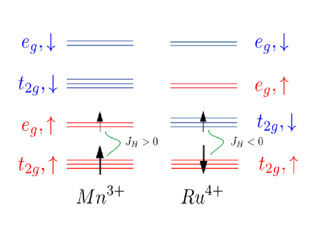
Figure 1: Schematically shown the energy band diagrams of $3d$ orbitals of $Mn^{3+}$ ions in LSMO (in left panel) and $4d$ orbitals of $Ru^{4+}$ ions in SRO (in right panel). The Hund’s coupling constant $J_{H}$ between the majority core spins and the minority spin is positive for $Mn^{3+}$ ions and negative for $Ru^{4+}$ ions. The spacing of energy levels are not drawn to scale.

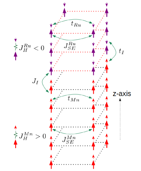
Figure 2: Schematic of the lattice model for LSMO/SRO superlattice based on Mn and Ru ions showing the super-exchange interactions ($J_{SE}^{Mn}$, $J_{SE}^{Ru}$, $J_{I}$), hopping parameters ($t_{Mn}$, $t_{Ru}$, $t_{I}$) and Hund’s couplings ($J_{H}^{Mn}$, $J_{H}^{Ru}$).

II Electronic Structures of Constituent Materials

Here, we discuss the relevant properties of the constituent layers in LSMO/SRO superlattice. LSMO is the optimally doped compound of $LaMnO_{3}$ with Sr in place of La, where three 3$d$ valence electrons of $Mn$ ion are occupied in $t_{2g}$ orbitals and the $e_{g}$ orbitals remain partially filled dagotto ; tokura . The average electron density $n$=0.7 is defined on the basis of occupancy of $e_{g}$ electrons. Three electrons in the $t_{2g}$ orbitals form a large core spin. We consider it as classical spin dagotto1 ${\bf|S|}$ and fix ${\bf|S|=1}$, which is coupled to the itinerant $e_{g}$ electrons spin via the Hund’s coupling dagotto1 ; zener ; yunoki ; pradhan . Delocalization of $e_{g}$ electrons results in ferromagnetic metallic state in the double exchange limit. Here, we assign Hund’s coupling to be large and positive, where itinerant electrons are aligned along the core spins ($3\uparrow,1\uparrow$) as shown in Fig. 1. This high spin configuration forms a total moment $\sim 3.7\mu_{B}$ as reported in experiments coey . Experimental observations show that LSMO has relatively a high ferromagnetic transition temperature ($T_{C}$ $\sim$ 360 K), negligible magnetic anisotropy and low coercive field steenbeck .

Coming to the next material, $SrRuO_{3}$ (SRO) is believed to be an itinerant ferromagnet with finite density of states at the Fermi level singh1 . Here, Ru is in the $Ru^{4+}$ state and all 4$d^{4}$ electrons are occupied in $t_{2g}$ orbitals ($3\uparrow,1\downarrow$) forming a low spin configuration state of total moment $2\mu_{B}$ which is close to the experimentally observed value $\sim 2.2\mu_{B}$ ning . Other experimental reports suggest that the $Ru^{4+}$ ion moment in SRO varies wildly depending upon the growth condition and found to be between 1.0-1.6 $\mu_{B}$ koster ; bushmeleva ; allen ; klein ; rondinelli . It is also known that compressively strained films exhibit enhanced saturated magnetic moments grutter . The lower value of magnetic moment indicates the itinerant nature of the $t_{2g}$ electrons. But, the coexistence of localized and itinerant magnetism can not be ruled out completely dodge ; shai ; kim . In our model Hamiltonian approach we consider $3\uparrow$ electrons as localized classical spin ${\bf|S|}$ which is Hund’s coupled to the $\downarrow$ itinerant electrons with an average system electron density $n=0.5$ which give rise to an effective moment $\sim$$2.5\mu_{B}$ ning ; chang . The sign of Hund’s coupling constant of low spin state $t_{2g}$ electrons in SRO is of opposite sign to that we assigned in LSMO (schematically shown in Fig. 1)). Although both LSMO and SRO have metallic conductivity at low temperatures SRO is relatively a bad metal toyota ; klein1 and the ferromagnetic transition temperature of SRO $T_{C}^{SRO}\sim$160 K longo ; koster which is much smaller than that of LSMO. Experimental observations show that SRO has larger magnetic anisotropy and higher coercive field in comparison to LSMO kanbayasi1 ; koster ; ziese3 . As a result, LSMO is a most preferred candidate for soft magnetic materials when coupled with hard ferromagnet like SRO, which has a relatively larger coercive field ziese ; ziese1 .

Based on above facts, where itinerant electrons are polarized opposite (parallel) to the direction of localized $t_{2g}$ core spins in SRO (LSMO), it is clear that the itinerant electrons prefer antiferromagnetic alignment (over the ferromagnetic alignment) of Mn and Ru $t_{2g}$ core spins at the interface to facilitate the hopping and gain kinetic energy chang . As a result the interfacial hopping drive the system to be less resistive in the antiferromagnetic configuration between the constituents ferromagnetic layers as compared to the ferromagnetic or paramagnetic configuration, in agreement with experiments takahashi . This shows that carrier-driven antiferromagnetic interaction is necessary to understand the one-to-one correspondence between magnetic and transport properties of the LSMO/SRO SLs along the hysteresis loop. It is worthwhile to note that in addition to this carrier-driven coupling, interfacial Mn-O-Ru bonds also generate a stronger antiferromagnetic super-exchange coupling at the interface ziese1 ; lee which is also needs to be incorporated.

III Model Hamiltonian and Methods

With the backdrop of the electronic structure and electron density we construct a reference one band classical Kondo lattice model Hamiltonian yunoki ; pradhan ; chakraborty in three dimensions to investigate the LSMO/SRO heterostructures as follows:

$$H=-t\sum_{<ij>,\sigma}(c_{i\sigma}^{\dagger}c_{j\sigma}+c_{j\sigma}c_{i\sigma}^{\dagger})\,-\,J_{H}\sum_{i}{\bf S}_{i}.{\bf\sigma}_{i}$$

$$+J\sum_{<ij>}{\bf S}_{i}.{\bf S}_{j}-A_{aniso}\sum_{i}(S_{i}^{z})^{2}$$

$$-\mu\sum_{i\sigma}c_{i\sigma}^{\dagger}c_{i\sigma}+\sum_{i\sigma}\epsilon_{i}c_{i\sigma}^{\dagger}c_{i\sigma.}$$

Here, the operator $c_{i\sigma}$ ($c_{i\sigma}^{\dagger}$) annihilates (creates) an itinerant electron with spin $\sigma_{i}$ at site $i$. $J_{H}$ is the Hund’s coupling between the $t_{2g}$ spins $\bf S_{i}$ and the itinerant electron spin ${\bf\sigma}_{i}$. We treat $\bf S_{i}$ to be classical variable and fix $\bf|S_{i}|=1$. $J$ is the antiferromagnetic super-exchange between the classical $S_{i}$ spins and $A_{aniso}$ is the strength of magneto-crystalline anisotropy. Chemical potential $\mu$ is tuned to set the average electron density of the overall system. $\epsilon_{i}$ is the onsite potential, essential for layered systems to keep the electron densities of both layers at their desired values. This term can be neglected for bulk systems. We perform our calculations in an external magnetic field $h$ by adding the Zeeman coupling $-{\bf h}\cdot\sum_{i}{\bf S}_{i}$ to the Hamiltonian.

We apply the exact diagonalization scheme to the itinerant electrons in the configuration of the fixed background of classical spins. The classical variables are annealed by Monte-Carlo procedure at each site where the proposed update is accepted or rejected by using metropolis algorithm starting with the random initial configuration. At each temperature we use 2000 system sweeps for annealing and in each sweep visit every lattice site sequentially and update the system. We measure physical parameters like magnetization after thermalizing the system at each 10 sweeps to avoid illicit self-correlation in the data. In order to access larger system size we use travelling cluster approximation kumar1 ; pradhan1 based Monte-Carlo scheme. We set up our model Hamiltonian calculations for m-LSMO/n-SRO heterostructure in 3D (N=$10\times 10\times 8$). Here, $m$($n$) represents the number of LSMO (SRO) planes with $m+n=8$. The size of the TCA cluster is taken to be $4\times 4\times 8$. Now onward, we assign different SL structures as $m/n$ SL, where $m$ LSMO planes constitute the LSMO layer and $n$ SRO planes constitute the SRO layer. In order to establish the bulk properties of individual LSMO and SRO layers we use $8\times 8\times 8$ system size.

IV Two sets of parameter values to mimic properties of bulk LSMO and SRO

In order to capture the essential physics of individual LSMO and SRO layers qualitatively, first we have to explore and find out two different sets of parameter values comprising of $t$, $J_{H}$, $J_{SE}$ and $A_{aniso}$. Keeping the basic properties of the constituent materials in mind, first we consider to build up the parameter space for the LSMO. We set $t_{Mn}=1$ and calculate all the observables in the unit of $t_{Mn}$. In order to mimic the ferromagnetic metallic state the Hund’s coupling constant is set in the double-exchange limit, $J_{H}^{Mn}=24$. We add a small antiferromagnetic super-exchange interaction putting $J_{SE}=0.01$ and neglect the magneto-crystalline anisotropy ($A_{aniso}^{Mn}=0$) which is much smaller than the SRO system.

Now, for SRO the parameters must be chosen in such a way that its physics relative to LSMO remain intact at least qualitatively e.g. the transition temperature $T_{C}^{SRO}<T_{C}^{LSMO}$, the coercive field $H_{C}^{SRO}>H_{C}^{LSMO}$ etc. Hence, we chose the hopping parameter $t_{Ru}=0.5$, the Hund’s coupling $J_{H}^{Ru}=-12$ and the magneto-crystalline anisotropy interaction $A_{aniso}^{SRO}=0.05$. The modality by which we assign the negative sign to $J_{H}^{Ru}$ is already discussed earlier (please see the discussion related to Fig. 1). A finite $A_{aniso}^{SRO}$ is essential to capture the higher value of coercive field $H_{C}$ in SRO compared to LSMO at low temperatures. We neglect any kind of super-exchange interaction in SRO. The electron densities are already fixed from the electronic structures of both materials, $n\sim 0.7$ for LSMO and $n\sim 0.5$ for SRO as outlined earlier. We tabulate the parameter sets for LSMO-like and SRO-like materials in Table.1.

System	Parameters to mimic LSMO and SRO like
	systems
LSMO	$n=0.7$, $J_{H}^{Mn}=24$, $t_{Mn}=1$, $J_{SE}^{Mn}=0.01$, $A_{aniso}^{LSMO}=0$
SRO	$n=0.5$, $J_{H}^{Ru}=-12$, $t_{Ru}=0.5$, $J_{SE}^{Ru}=0$, $A_{aniso}^{SRO}=0.05$

Table 1: Various parameters to model LSMO and SRO like systems. For LSMO/SRO SLs we set $J_{I}=0$ and $t_{I}=0.75$ unless otherwise mentioned.

Next, the task is to calculate and establish the essential properties of LSMO-like and SRO-like materials separately using the parameter sets given in Table-1. We present the magnetization $M$ $=1/N\sum_{i}S_{z}^{i}$ data in Fig. 3(a), where $N$ is number of sites and $S_{z}$ is the $z$ component of the classical spins. The magnetization with temperature graphs show that the ground state is ferromagnetic for both the materials with $T_{C}^{LSMO}>T_{C}^{SRO}$. In experiments, the $T_{C}^{LSMO}$ is measured to be as large as twice of $T_{C}^{SRO}$. We agree that our calculations do not reflect this fact quantitatively. It is important to note here that the magneto-crystalline anisotropy is mainly a low temperature effect. So taking $A_{aniso}^{SRO}=0$ above $T_{C}$ and $A_{aniso}^{SRO}=0.05$ below $T_{C}$ (keeping all other parameters fixed as in (a)) we present the calculations for SRO in Fig. 3(b). Now, the ferromagnetic $T_{C}^{SRO}$ is reduced and consequently the gap between the $T_{C}$ of the two systems widens, which is a better match to the experimental results. In this work, most of the calculations are carried out below the ferromagnetic $T_{C}$ of SRO ($T_{C}^{SRO}$) and high temperature means $T\lesssim T_{C}^{SRO}$, similar to experiments. In that spirit we use the parameter space employed in (a) for both LSMO and SRO to avoid confusions. In the inset of Fig. 3(a) we show the resistivity for both the systems. We obtain the resistivity by calculating the $dc$ limit of the conductivity as determined by the Kubo-Greenwood formula mahan-book ; kumar2 ; pradhan2 . Our calculations show that both systems are metallic at low temperature which agrees with the experimental results.

Next, we compare the coercive field $H_{C}$ of both the systems in Fig. 3(c). Our calculations shows that $H_{C}^{LSMO}<H_{C}^{SRO}$ at low temperature ($T=0.02$) giving rise to a combination of hard and soft ferromagnets as required for modelling the superlattice (SL). On the other hand, $H_{C}^{LSMO}$ is comparable to $H_{C}^{SRO}$ at intermediate temperatures [see  3(d)] as we move close to $T_{C}^{SRO}$. So, the two sets of parameters that we assigned to LSMO-like and SRO-like materials capture qualitatively the essential physics that is required to investigate their superlattices. Hence, we call them LSMO and SRO in our further analysis. In addition, in Fig. 3(a), using the dotted line, we have shown that the M-T data is no different if one uses $J_{H}^{Ru}=-9$. We also confirm that $H_{C}^{SRO}$ remains same for both $J_{H}^{Ru}$ = -9 and -12 (not shown in figure). What would happen to the M-h curve if we take a larger anisotropy constant $A_{aniso}^{SRO}=0.1$ instead of $A_{aniso}^{SRO}=0.05$, particularly at low temperatures? Obviously the $H_{C}^{SRO}$ gets enhanced further as shown using the dotted line in Fig. 3(c).

Figure 3: Displays the bulk properties of individual LSMO and SRO systems computed using the parameter sets listed in Table-1. (a) and (b) present the magnetization M vs temperature T results with $A_{aniso}^{SRO}$=0.05 in the whole temperature range and with $A_{aniso}^{SRO}$=0.05 (0.00) below (above) $T_{C}^{SRO}$, respectively. In both cases $T_{C}^{LSMO}>T_{C}^{SRO}$ with a reduced value of $T_{C}^{SRO}$ for $A_{aniso}^{SRO}$=0.0 above $T_{C}^{SRO}$ case. Also shown the M vs T of SRO-like materials for $J_{H}=-9$ using the dashed line. Most of our calculations are performed for $T<T_{C}^{SRO}$ and we employ the parameters used in (a) to model LSMO and SRO in rest of our calculations. Inset shows that both LSMO and SRO are metallic at low temperatures. (c) and (d) show the M vs applied field $h$ hysteresis loops of LSMO-like and SRO-like materials at low temperature $T=0.02$ and moderate temperature $T=0.05$, respectively. The arrows indicate the field sweep direction. Clearly, Coercive field of SRO $H_{C}^{SRO}>H_{C}^{LSMO}$ at $T=0.02$, but comparable to each other at $T=0.05$. Legends are same in panels (a), (c) and (d). Also, we show the M-h hysteresis loop for SRO like materials for $A_{aniso}^{SRO}$=0.1 in (c) using dashed lines.

In experiments, during the magnetic hysteresis measurements (at low temperature) of LSMO/SRO SLs magnetization of the SRO layer is pinned up to moderate field strength for positive field cooled system, whereas the LSMO layer switches its orientation during field sweep. This is a consequence of higher coercive field of SRO as compared to LSMO. In addition, a positive exchange bias is also observed in experiments below the ferromagnetic $T_{C}^{SRO}$ which is believed to be a consequence of anti-ferromagnetic inter-layer coupling ziese1 . In fact, this antiferromagnetic interlayer coupling plays a significant role in transport and magnetic properties of the LSMO/SRO SLs. Here, it is an interesting scenario where interlayer coupling turns out to be antiferromagnetic although the constituent layers themselves have dominant ferromagnetic interactions among the core spins. This is explained using the transformed interfacial bond arrangements and resulting interfacial charge transfer. Density functional calculations suggest that the bond angle Mn-O-Ru at the interface drives an antiferromagnetic super-exchange coupling ziese1 ; lee , whose strength would be different from the super-exchange interaction within either layer. The impact of interfacial electronic charge transfer is two fold: (i) it modifies the antiferromagnetic super-exchange interaction and (ii) induces an antiferromagnetic interaction via carrier driven process at the interface, as discussed earlier. This charge carrier mediated coupling will very much depend upon the modified hopping parameter $t_{I}$ at the interface. In fact, the strength of charge transfer driven antiferromagnetic coupling would be larger for $t_{I}=t_{Mn}=1$ as compared to that of $t_{I}=t_{Ru}=0.5$.

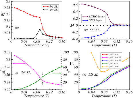
Figure 4: Magnetic and transport properties of LSMO/SRO SLs: (a) Variation of M with T for the 5/3 SL and 4/4 SL showing the sign of onset of antiferromagnetic interfacial coupling at $T\sim 0.1$. (b) M vs T of individual LSMO and SRO layers for 5/3 SL confirms the fact that at low temperatures both the layers are aligned ferromagnetically with antiferromagnetically coupled at the interface. (c) Variation of out-of-plane resistivity $\rho_{z}$ and effective hopping parameter $t_{eff}$ with temperature for the 5/3 SL showing an insulator-metal transition at $T=0.1$. The sharp change in $t_{eff}$ at $T=0.1$ is due to the gain in the kinetic energy of the carriers in the SL. This corroborates the fact that antiferromagnetic interfacial coupling (shown in (b)) drives the system towards a metallic phase. (d) Variation of $\rho_{z}$ vs $T$ for different combinations of interfacial hopping parameter and interfacial super-exchange interaction ($t_{I}$, $J_{I}$) values depict that suppressed carrier hopping across the interface ($t_{I}$=0.25) negates the insulator-metal transition.

V Establishing the antiparallel alignment of LSMO and SRO layers

It is generally assumed that the inter-layer coupling decides the overall properties of the heterostructures. So, we start the SL structure calculations with understanding the nature of interfacial interaction in 5/3 and 4/4 superlattices (SLs). These notions of SL structures are already discussed. To maintain the desired electron densities in both the layers one has to be chosen the relative on-site potential $\epsilon$ accordingly. $\epsilon$ takes the value $\bigtriangleup$ (0) in LSMO (SRO) layer. And, we found that for $\bigtriangleup=10.7$ the LSMO and SRO layers maintain the electron densities 0.7 and 0.5, respectively, in both 5/3 SL and 4/4 SL systems. LSMO and SRO layers are coupled at the interface via hopping parameter $t_{I}$ and the super-exchange interaction $J_{I}$. We set $t_{I}$=0.75 and $J_{I}=0$ unless otherwise mentioned. This will help us to first analyze the effects of the carrier driven interfacial antiferromagnetic coupling. In subsequent calculations the consequence of super-exchange coupling is emphasized wherever necessary.

We measure the magnetization of the 5/3 and the 4/4 SLs by cooling from high temperature $T=0.16$ in a very small external field $h=0.002$ [see Fig. 4(a)]. In both cases the magnetization starts to increase at $T\sim 0.11$, which is attributed to the ferromagnetic alignment of the high $T_{C}$ constituent LSMO layer. At $T\sim 0.09$ the magnetization decreases for 4/4 SL, whereas the slope of magnetization curve changes abruptly in case of 5/3 SL. These results indicate that the SRO layer starts to align ferromagnetically but in opposite orientation to LSMO layer at $T=0.09$. In order to verify this fact we plot the magnetization of embedded LSMO and SRO layers separately for 5/3 SL in Fig. 4(b), which we found to be consistent with the results presented in Fig. 4(a). So, the antiferromagneic interaction at the interface drives the layers to align antiferromagnetically at low temperatures. Now the question arises: does this antiferromagnetic alignment at $T$ $\sim 0.09$ leads to a metallic state according to our hypothesis, presented earlier, where we argued that antiferromagnetic alignment at the interface facilitate the delocalization of charge carriers. To check this we calculated the out-of-plane resistivity $\rho_{z}(T)$ and presented in Fig. 4(c). The resistivity depicts an insulator-metal transition around $T\sim 0.1$ (indicated by black arrow) where both layers start to align antiferromagnetically with each other as shown in Fig. 4(a) and (b). This ensures that the LSMO/SRO SL systems with antiferromagnetic interfacial coupling are metallic in nature. In order to establish the correspondence between resistivity and gain in kinetic energy we calculate the effective hopping white ; mondaini

$$t_{eff}=\langle\sum_{j,\sigma}(c_{j,\sigma}^{\dagger}c_{j+z,\sigma}+c_{j+z,\sigma}c_{j,\sigma}^{\dagger})\rangle$$

of 5/3 SL, where angular bracket represents the expectation value. The $t_{eff}$ vs temperature shows a sharp change at $T=0.1$ indicating that gain in kinetic energy of the SL system gets enhanced at the same temperature where both LSMO and SRO layers start to align antiferromagnetically. So our $t_{eff}(T)$ and $\rho_{z}(T)$ results compliment each other.

In order to establish the fact that the carrier-driven antiferromagnetic coupling between the two ferromagnetic layers steers the SL towards a metallic (insulating) state when LSMO and SRO are aligned in anti-parallel (parallel) configuration, as seen in experiments, we calculate the magnetic and transport properties using different combinations of $t_{I}$ (interfacial hopping parameter) and $J_{I}$ (interfacial super-exchange interactions). For varying $J_{I}$ with a fixed $t_{I}=0.75$ we did not find any variation in the resistivity curve as shown in Fig. 4(d). But for small values of $t_{I}$ (with fixed $J_{I}=0$) the system does not go to a metallic state at low temperatures although LSMO and SRO layers align antiferromagnetically (not shown in figure). This shows that a reasonable interfacial hopping that also drives the antiferromagnetic interaction is necessary to understand the magneto-transport properties of LSMO/SRO SLs.

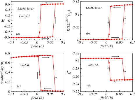
Figure 5: Focuses on the minor hysteresis loops (the hysteresis of only LSMO layer) of 5/3 SL at low temperature $T=0.02$. Here, the applied field is restricted within a region such that only the magnetization of LSMO flips its direction, leaving the SRO layer pinned along the up direction. The arrows indicate the field sweep direction. (a) Shows the positive exchange bias of the soft magnetic layer LSMO with a shift of the M-h hysteresis loop to the right of the zero field axis. (b) Displays the hysteresis of spin-up density of states of LSMO layer at the Fermi level ($D_{\uparrow}^{LSMO}(\varepsilon_{F})$) which follows magnetic hysteresis curve shown in (a). (c) Hysteresis of conductivity shows that the SL is more conducting for oppositely oriented LSMO and SRO layers as compared to their parallel configuration. (d) Hysteresis of effective hopping parameter $t_{eff}$ follows conductivity loop which corroborate the fact that the carriers are more mobile in antiparallel configuration as compared to the parallel configuration of both layers across the interface.

VI Positive Exchange Bias

We have established the essential properties of LSMO, SRO and their SLs qualitatively. Now, we come to the key calculation of the article, where we measure the magnetic hysteresis M-h loop. We start with 5/3 SL at low temperature $T=0.02$. First, we cool down the SL from high temperature to $T=0.02$ under an external magnetic field $h=0.1$ and then measure the M-h loop. The field cycle of $h$ loop is restricted to $\pm$0.1, so that the magnetization of the SRO layer remains in the up direction and does not flip at all. We will see in next section that SRO flips its direction beyond $h=-0.1$. Here, the aim is to analyze the minor hysteresis loop of the SL, which is the full hysteresis loop of the embedded LSMO layer. We have presented the variation of magnetization of LSMO layer in Fig. 5(a). For $h=+0.1$ LSMO and the SRO layers are aligned ferromagnetically along the field direction. As we decrease the magnetic field strength the magnetization of the LSMO layer flips its direction at a small +ve field (LSMO$\uparrow$ SRO$\uparrow$ to LSMO$\downarrow$ SRO$\uparrow$). Primarily, there are two reasons of this flip: (i) Coercive field of LSMO is smaller than SRO ($H_{C}^{LSMO}<H_{C}^{SRO}$) as shown in Fig. 3(c) and (ii) the interfacial antiferromagnetic coupling who wins over the low field strength in aligning the LSMO layer in its favour. While sweeping back the field from $h=-0.1$, a higher field strength ($h=0.07$) is required to overcome the antiferromagnetic inter-layer coupling and flip back the LSMO magnetization along the field direction. As a result, the hysteresis loop of the LSMO layer shifts towards the positive field axis giving rise to a positive exchange bias. In addition, we have calculated the spin-resolve density of states (DOS) at the Fermi level ($\varepsilon_{F}$) of the LSMO layer and plot the spin up density of states $D_{\uparrow}^{LSMO}(\varepsilon_{F})$ in Fig. 5(b), which perfectly follows the LSMO magnetic hysteresis loop shown in Fig. 5(a). This shows that if the carriers are perfectly aligned to the core spins the DOS of the soft ferromagnet can be used as a parameter to track the magnetization flipping in LSMO/SRO like SLs.

We already discussed that the carriers will be more delocalized (localized) across the interface in SL structure when the magnetic moments in LSMO and SRO layers are aligned antiferromagnetically (ferromagnetically) with each other. To check this fact, we have calculated the $dc$ conductivity throughout the magnetic hysteresis loop and found that the SL is more conducting in the anti-parallel configuration as compared to the parallel configuration of LSMO and SRO layers as shown in Fig. 5(c). We also show that the hysteresis loop of the effective hopping $t_{eff}$ [see Fig. 5(d)] is very similar to conductivity hysteresis loop, corroborating the fact that carriers are more mobile across the interface in anti-parallel configuration (LSMO$\downarrow$ SRO$\uparrow$) as compared to parallel orientation (LSMO$\uparrow$ SRO$\uparrow$).

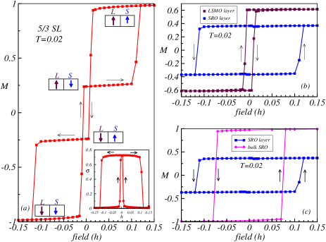
Figure 6: Magneto-transport properties along the magnetic hysteresis measurements for 5/3 SL at $T=0.02$: (a) The complete magnetic hysteresis curve shows a centrally inverted hysteresis loop with negative coercivity and negative remanence as observed in the experiment ziese2 . Relative magnetization of LSMO and SRO layers (LSMO as L and SRO as S) is illustrated schematically. Inset shows that the conductivity in anti-parallel configuration is larger than that of the parallel configuration along the hysteresis loop. (b) Separate plots of magnetic hysteresis curves of the embedded SRO and LSMO layers depict that the SRO magnetization behaves conventionally, in contrast to the LSMO magnetization which is inverted. (c) The magnetic hysteresis of the embedded SRO layer is compared with that of the free standing bulk system [replotted as in Fig. 3(c)]. The coercive field $H_{C}$ of embedded SRO layer is larger than that of the bulk SRO due to the interfacial coupling, which resist the layer to flip at $H_{C}^{SRO(bulk)}$.

VII Inverted Hysteresis loop

We now investigate the full hysteresis loop of the 5/3 SL at low temperature $T=0.02$. Here and in later sections all the calculations are carried out after cooling down the SL in the external field $h_{cooling}$= + 0.15, which is higher than the $H_{C}^{SRO}$. At this forward saturation field strength the magnetizations of both LSMO and SRO layers are aligned parallel to the external field. It is also important to remember that the SRO layer (LSMO layer) acts as a hard (soft) ferromagnet at $T=0.02$. So, by decreasing the field from $h$=+0.15 towards $h$=-0.15, first the LSMO layer reverses its magnetization at small but finite positive fields giving rise to a negative remanence. Then the SRO layer flips its magnetization at a larger external magnetic field of opposite polarity (at $h\sim-0.11$) as shown in Fig. 6(a). Now, traversing the field back from $h$=-0.15 the LSMO magnetization flips first at a small negative field resulting in a negative remanence and then SRO flips at a higher positive field (at $h\sim 0.11$) strength, giving rise to a central inverted hysteresis loop (IHL) which is very similar to the experimental results ziese2 . For clarity, we have also plotted the magnetic hysteresis of individual LSMO and SRO layers embedded in SL in Fig. 6(b). The SRO layer shows a conventional hysteresis loop, but LSMO layer depicts an inverted loop. This is because the interfacial antiferromagnetic coupling steers LSMO layer to align opposite to field direction by overcoming the external field energy to establish the antiferromagnetic configuration giving rise to a negative remanence. So, the full M-h hysteresis loop at low temperature reveals the striking magnetization reversal process that is absent in the minor hysteresis loop of the SL that we presented in the previous section. The SL system is found to be metallic (insulating) along the hysteresis loop where LSMO and SRO are aligned in anti-parallel (parallel) configuration as shown in the inset of Fig. 6(a). This fact is in good agreement with experimental results takahashi .

Figure 7: Comparison of magnetic hysteresis loops of 5/3 SLs at $T=0.02$ with (a) variation of the interfacial super-exchange interaction $J_{I}$ at fixed value of interfacial hopping parameter $t_{I}=0.75$ and (b) variation of $t_{I}$ at fixed $J_{I}=0$. Both $J_{I}$ and $t_{I}$ enhance the interfacial coupling strength. So, the width of the central IHL broadened with increasing $J_{I}$ and/or $t_{I}$. Inset: IHL is absent for the parameters set $(t_{I},J_{I})=(0.5,0)$, which indicates that a reasonable strength of the interfacial antiferromagnetic coupling is essential to realize the inverted hysteresis feature.

In addition, we compared the magnetic hysteresis of the embedded SRO layer with the bulk SRO system at $T=0.02$ in Fig. 6(c). The coercive field of SRO in SL is larger than that of the bulk SRO, $H_{C}^{SRO(SL)}>H_{C}^{SRO(bulk)}$. The earlier flipping of LSMO layer as shown in Fig. 6(a) favours the interfacial antiferromagnetic coupling which opposes the SRO layer to flip in the field direction up to a certain field strength that is larger than $H_{C}^{SRO(bulk)}$. As a result, relatively a large field of opposite polarity is required to flip the SRO layer as compared to its bulk counterpart.

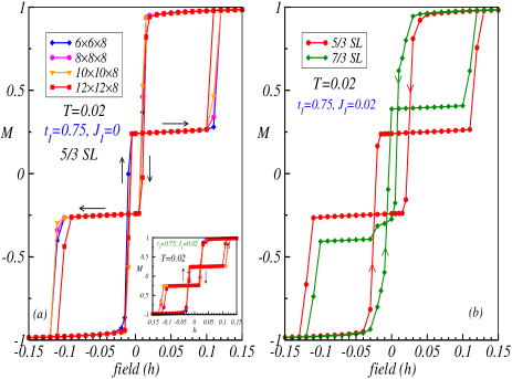
Figure 8: The stability of the IHL with different system sizes: (a) Magnetic hysteresis along with the IHLs for four different system sizes are seen to be almost indistinguishable from each other. All systems are belong to the 5/3 SL structure. Inset: The IHLs are also very stable for $J_{I}=0.02$. (b) Shows the shrinking of the width of the IHL for 7/3 SL structure (system size: $10\times 10\times 10$) as compared to the 5/3 SL due to thicker LSMO layer (7 planes), which flips its magnetization at a lower applied field strength as compared to the thinner LSMO layer (5 planes).

It is earlier mentioned that primarily there are two sources of inter-layer antiferromagnetic interaction: (i) carrier-mediated antiferromagnetic coupling and (ii) Mn-O-Ru bond driven super-exchange coupling ($J_{I}$). In all calculations presented till now, we incorporated only the first type of interaction among the core spins at the interface for analyzing the hysteresis loop. Now, we consider both interactions and investigate the inverted hysteresis loop in Fig. 7 to emphasize the effect of Mn-Ru direct super-exchange coupling. We compare the M-h hysteresis loops for different super-exchange coupling strengths $J_{I}$=0 and 0.02 at fixed $t_{I}=0.75$ at low temperature $T=0.02$ in Fig. 7(a). The central inverted part of the hysteresis loop is seen to be more prominent for $J_{I}$=0.02. The reason is the enhancement of overall (effective) antiferromagnetic interaction at the interface that facilitate the rotation of magnetization (from up to down direction) of the LSMO layer at a larger positive applied field. The carrier-mediated antiferromagnetic coupling can also be enhanced (for fixed $J_{I}$=0) by increasing the inter-layer hopping parameter $t_{I}$ to 1 instead of 0.75, which can be understood from the inverted part of the hysteresis loop shown in Fig. 7(b). The inter-layer coupling strength decreases considerably in case of suppressed carrier hopping ($t_{I}=0.5$), which results in a conventional hysteresis loop without any inverted part (see inset of Fig. 7(b)). These results clearly show the crucial role of the interfacial antiferromagnetic coupling in generating the central inverted hysteresis loop.

Next, we demonstrate the stability of the inverse hysteresis loop for different system sizes. In Fig. 8(a) shows the M-h hysteresis loops for four different system sizes, namely N=$6\times 6\times 8$, $8\times 8\times 8$, $10\times 10\times 8$ and $12\times 12\times 8$ at low temperature $T=0.02$. Here, we have modified only the size of the planes keeping the thickness of the SLs and individual layers fixed. So all these calculations are for different sizes but each one of them falls under the 5/3 SLs group. Interestingly, the overall hysteresis loops including the central inverted parts are hardly distinguishable from each other for all four cases. This shows that the magnetic properties, we discussed for the system size N=$10\times 10\times 8$, remains very robust without any significant size effect. We have also shown that the magnetic hysteresis loop remains unaffected by varying the size of the system for $J_{I}=0.02$ (see the inset of Fig. 8(a)).

Switching of LSMO moments within small magnetic field strengths results in the IHL for 5/3 SL at $T=0.02$ and $J_{I}$=0, discussed in Fig. 6. Tuning on the inter-layer super-exchange antiferromagnetic interaction ($J_{I}$=0.02) the central IHL becomes more prominent (see Fig. 7). What will happen to the central IHL if one varies the thickness of the LSMO layer, keeping the SRO thickness fixed? To check this, we considered: (i) 7/3 SL with a $10\times 10\times 10$ lattice and (ii) 9/3 SL with a $10\times 10\times 12$ lattice for $J_{I}$=0.02. Keeping the thickness of SRO layer fixed if we increase the LSMO layer thickness it is clearly visible that the area of the central inverted loop part shrinks (see Fig. 8(b)). And, if we further increase it then the IHL vanishes and conventional loop reappears for 9/3 SL (not shown in the figure). In this case the magnetization of the LSMO layer flips below $h=0$ resulting in the disappearance of IHL. This is because the thick LSMO layer does not prefer to get rotated easily (rotation is based on the interfacial antiferromagnetic coupling) as compared to the thin LSMO layer against the magnetic field energy. These results indicate the importance of relative thicknesses of the constituent layers to realize the IHL in SLs.

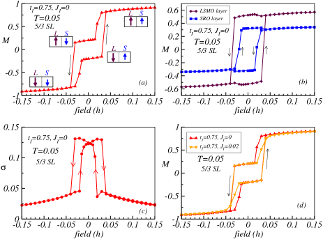
Figure 9: Presents the magneto-transport properties for 5/3 SL at intermediate temperature $T=0.05$, where the coercive fields of bulk LSMO and SRO are comparable to each other (see Fig. 3(d)). We set $J_{I}=0$. (a) M-h hysteresis loop shows a two-step switching process, but without any central inverted part. (b) Clarifies the switching process with separately plotted the M-h data of embedded LSMO layer. (b) along with (a) ensure that the magnetization of SRO layer flips first which is followed by LSMO layer. In fact, embedded SRO layer shows inverted hysteresis feature. (c) Shows that conductivity in parallel orientation remains smaller than that of the anti-parallel configuration along the M-h hysteresis loop. (d) Additional interfacial super-exchange coupling $J_{I}=0.02$ does not change the qualitative features of the two-step flipping process of M-h hysteresis loop.

VIII Unconventional three-step flipping process along the hysteresis loop

The temperature dependent hard or soft nature of LSMO and SRO results in unconventional and interesting magnetic hysteresis loops in LSMO/SRO SLs at low temperatures. We have calculated and discussed, in detail, the hysteresis loop at low temperature where the coercive fields of LSMO and SRO layers are quite different from each other. What if the coercive fields of two materials are comparable to each other? How does the magnetic hysteresis loop will behave in such a scenario? For this we have to study the M-h loops at high temperatures. Before going to analyze high temperature calculations it would be interesting to explore the intermediate temperature regime where the coercive fields of the constituent layers are already comparable to each other (see Fig. 3(d) for $T=0.05$). Hence, we plot the M-h magnetic hysteresis curves for 5/3 SL at $T=0.05$ in Fig. 9(a), which shows a two-step process as in the low temperature case. In high field strength both layers are aligned along the field direction. Sweeping from the forward to the reverse saturation field the SRO layer flips first at a small +ve field creating a ferrimagnetic SL magnetization and ultimately both layers align along the field direction (LSMO$\uparrow$ SRO$\uparrow$ to LSMO$\uparrow$ SRO$\downarrow$ to LSMO$\downarrow$ SRO$\downarrow$) at saturation field. This flipping scenario is more clear in Fig. 9(b) where we have plotted the magnetization of the individual LSMO and SRO layers. It is clear that LSMO layer is the second one to switch its magnetization direction. In fact, the flips of only SRO layer depict an inverted hysteresis loop similar to the LSMO layer presented in Fig. 6(b) for low temperatures. The inverted part is not visible for whole SL structure at $T=0.05$ due to the smaller effective magnetic moment in SRO layer which happens to flip first in this case. So, to visualize the central inverted hysteresis loop it is necessary that the higher moment layer should flip first and give a negative remanence. The $dc$ conductivity in Fig. 9(c) shows that the conductivity in parallel configuration remains smaller compared to the anti-parallel configuration, similar to low temperature case. The two-step switching process as a function of the magnetic field remains intact even modifying the inter-layer interaction by tuning on the super-exchange mediated coupling to $J_{I}=0.02$ (see Fig. 9(d)).

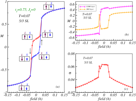
Figure 10: Displays the magneto-transport properties of 5/3 SL at high temperature $T=0.07$ (close to $T_{C}^{SRO}$). (a) M-h hysteresis measurements depict the unconventional three-step magnetization flipping process, qualitatively similar to the experimental results ziese2 . (b) The magnetization switching of the embedded individual LSMO and SRO layers during M-h cycle confirm the three-step flipping. (c) Conductivity measurements along the hysteresis loop show that layers in the anti-parallel configuration are more conducting than that in the parallel orientation. But, their difference is reduced at high temperature as compared to low temperature.

At both low and intermediate temperature a two-step switching process is observed. LSMO (SRO) flips first at $T=0.02$ ($=0.05$) and generates a ferrimagnetic configuration of the magnetic moments in the SL in the intermediate-step of M-h hysteresis curve. But at high temperature, close to $T_{C}^{SRO}$, an unconventional three-step switching process (LSMO$\uparrow$ SRO$\uparrow$ to LSMO$\uparrow$ SRO$\downarrow$ to LSMO$\downarrow$ SRO$\uparrow$ to LSMO$\downarrow$ SRO$\downarrow$) is observed in the experiment ziese2 . Here, the SRO layer flips first at a positive low field followed by a switching of the overall ferrimagnetic SL magnetization in negative low fields and a further switching of the SRO layer to align along the field direction. In order to understand this complicated unconventional three-step process we study the $M-h$ hysteresis curve at $T=0.07$ in Fig. 10(a). This temperature is just below the $T_{C}$ of SRO, similar to the experimental set up. During the field sweep starting from $h$=+0.15, sweeping from the forward to the reverse saturation field, the SRO layer switches its direction first, as in case of $T=0.05$, making the ferrimagnetic SL. This ferrimagnetic configuration changes its overall direction at $h\sim-0.05$. Then, further going beyond this field strength both the layers orient in the field direction. The three-step flipping process is also observed during traversing sweep which emphasizes the stability of the second ferrimagnetic configuration (LSMO $\downarrow$ SRO$\uparrow$) along the hysteresis loop. This three-step flipping process is depicted in Fig. 10(b) where we have plotted the magnetization of the individual layers (plotted only for sweeping from the forward to the reverse saturation field). The carrier mediated antiferromagnetic interaction at the interface for fixed $J_{I}=0$ plays the vital role in stabilizing the both ferrimagnetic phases which we will discuss soon. Due to the high operating temperature value the saturation magnetization of both the layers are much smaller than the saturation magnetization values observed for earlier calculations. Also the $dc$ conductivity in parallel configuration is found to be only marginally smaller than the anti-parallel configuration (see Fig. 10(c)).

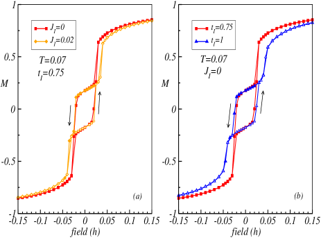
Figure 11: Demonstrates the effect of interfacial antiferromagnetic coupling on the three-step flipping process of 5/3 SL at high temperature $T=0.07$. In (a) the interfacial super-exchange interaction $J_{I}$ is varied with keeping the interfacial hopping parameter fixed at $t_{I}=0.75$, and in (b) $t_{I}$ is varied with fixed $J_{I}=0$. The interfacial coupling strength increases with increasing $J_{I}$ and/or $t_{I}$. So in both cases the three-step flipping process is more prominent for higher values of $J_{I}$ and $t_{I}$.

In the three-step switching process (shown in Fig. 10(a)), although the reversal of ferrimagnetic SL configuration is observed, the second ferrimagnetic configuration (LSMO$\downarrow$ SRO$\uparrow$) withstands over a very narrow magnetic field window. In order to show that the interfacial antiferromagnetic interaction plays a significant role in stabilizing this ferrimagnetic phases we incorporated the super-exchange interaction and calculated the magnetic hysteresis loop of the SL at $T=0.07$. The three-step switching process is found to be more prominent, particularly the second ferrimagnetic configuration (LSMO$\downarrow$ SRO$\uparrow$) for $J_{I}$=0.02 as shown in Fig. 11(a). This indicates that the LSMO layer prefers to orient along the field direction at a particular small negative field value for which ferrimagnetic SL configuration reverses to maintain the antiferromagnetic interaction between the two layers at the interface. This is also supported from the results obtained from varying the inter-layer hopping parameter $t_{I}$ with fixed $J_{I}=0$. As the carrier driven antiferromagnetic coupling at the interface increases with $t_{I}$ the three-step magnetic flipping process is more prominent for $t_{I}$=1 as compared to $t_{I}$=0.75 (see Fig. 11(b)). But surprisingly the magnetic switching remains a two-step process for $t_{I}$=0.5 due to insufficient strength of the interfacial antiferromagnetic coupling. Here, if we incorporate a large super-exchange interaction ($J_{I}=0.05$) then only the three-step flipping process is recovered (not shown in figure). These results establish that a reasonable strength of interfacial antiferromagnetic coupling (comprised of carrier driven and bond driven) between LSMO and SRO is required to realize the three-step switching process at high temperature as seen in the experiments.

IX CONCLUSIONS

In this work we investigated the interfacial antiferromagnetic interaction driven complex magneto-transport phenomena observed in LSMO/SRO superlattices (SLs) within a one-band double exchange model using a Monte-Carlo technique based on travelling cluster approximation. We have considered the appropriate magneto-crystalline-anisotropy interaction and super-exchange interactions terms of LSMO and SRO (the constituent materials) in the model Hamiltonian. Also, our calculations incorporate: (i) the carrier-driven and (ii) the bond-mediated super-exchange interfacial antiferromagnetic interactions between Mn and Ru to demonstrate the vital role of the interfacial coupling in deciding the magneto-transport properties along the hysteresis loop. Our conductivity calculations show that the anti-aligned core spins at the interface prompt the carrier hopping between both layers to gain kinetic energy and consequently steers the SL system towards a metallic (less resistive) phase. On the other hand, the SL is found to be in a less metallic or insulating state when the LSMO and SRO layers are aligned in the same direction. Hence, the system undergoes metal-insulator or insulator-metal transition upon varying the temperature and/or the applied magnetic field. Interestingly, by invoking the antiferromagnetic coupling at the interface, we explained the exchange bias effect and inverted hysteresis loop at low temperatures, and unconventional three-step flipping mechanism at high temperatures (close to ferromagnetic $T_{C}$ of SRO), which are in good agreement with the experimental results. In addition, our calculations establish that the carrier-driven antiferromagnetic interaction is one of the necessary ingredient to understand the one-to-one correlation between the magnetic and the transport properties of LSMO/SRO SLs observed in experiments.

References

- (1) J. B. Goodenough, Chem. Mater. 26, 820 (2014).
- (2) D. I. Khomskii, J. Magn. Magn. Mater. 306, 1 (2006).
- (3) P. Zubko, S. Gariglio, M. Gabay, P. Ghosez, and J. M. Triscone, Annu. Rev. Condens. Matter Phys. 2, 141 (2011).
- (4) H. Y. Hwang, Y. Iwasa, M. Kawasaki, B. Keimer, N. Nagaosa, and Y. Tokura, Nat. Mater. 11, 103 (2012).
- (5) J. Mannhart and D. G. Schlom, Science 327, 1607 (2010).
- (6) M. Fiebig, T. Lottermoser, D. Meier, and M. Trassin, Nat. Rev. Mater. 1, 1 (2016).
- (7) K. F. Wang, J. M. Liu, and Z. F. Ren, Adv. Phys. 58, 321 (2009).
- (8) N. Feng, W. Mi, X. Wang, Y. Cheng, and U. Schwingenschlogl, ACS Appl. Mater. Interfaces 7, 10612 (2015).
- (9) S. M. Wu, S. A. Cybart, P. Yu, M. D. Rossell, J. X. Zhang, R. Ramesh, R. C. Dynes, Nat. Mater. 9, 756 (2010).
- (10) P. Yu, J. S. Lee, S. Okamoto, M. D. Rossell, M. Huijben, C. H. Yang, Q. He, J. X. Zhang, S. Yang, M. J. Lee, Q. M. Ramasse, R. Erni, Y. H. Chu, D. A. Arena, C. C. Kao, L. W. Martin, R. Ramesh, Phys. Rev. Lett. 105, 027201 (2010).
- (11) A. P. Ramirez, Journal of Physics: Condensed Matter 9, 8171 (1997).
- (12) F. Y. Bruno, J. Garcia-Barriocanal, M. Varela, N. M. Nemes, P. Thakur, J. C. Cezar, N. B. Brookes, A. Rivera-Calzada, M. Garcia-Hernandez, C. Leon, S. Okamoto, S. J. Pennycook, and J. Santamaria, Phys. Rev. Lett. 106, 147205 (2011).
- (13) J. Garcia-Barriocanal, J. C. Cezar, F. Y. Bruno, P. Thakur, N. B. Brookes, C. Utfeld, A. Rivera-Calzada, S. R. Giblin, J. W. Taylor, J. A. Duffy, S. B. Dugdale, T. Nakamura, K. Kodama, C. Leon, S. Okamoto, and J. Santamaria, Nature Commun. 1, 82 (2010).
- (14) J. Hoffman, I. C. Tung, B. B. Nelson-Cheeseman, M. Liu, J. W. Freeland, and A. Bhattacharya, Phys. Rev. B 88, 144411 (2013).
- (15) C. He, A. J. Grutter, M. Gu, N. D. Browning, Y. Takamura, B. J. Kirby, J. A. Borchers, J. W. Kim, M. R. Fitzsimmons, X. Zhai, V. V. Mehta, F. J. Wong, and Y. Suzuki, Phys. Rev. Lett. 109, 197202 (2012).
- (16) J. Krishna Murthy and P. S. Anil Kumar, Sci. Rep. 7, 6919 (2017).
- (17) A. Bhattacharya, Annu. Rev. Mater. Res. 44, 65 (2014).
- (18) P. Anil Kumar and D. D. Sarma, Appl. Phys. Lett. 100, 262407 (2012).
- (19) S. Emori, U. S. Alaan, M. T. Gray, V. Sluka, Y. Chen, A. D. Kent, and Y. Suzuki, Phys. Rev. B 94, 224423 (2016).
- (20) M. Wahler, N. Homonnay, T. Richter, A. Mueller, C. Eisenschmidt, B. Fuhrmann, and G. Schmidt, Sci. Rep. 6, 28727 (2016).
- (21) M. Gibert, P. Zubko, R. Scherwitzl, J. Iniguez, and J. Triscone, Nat. Mater. 11, 195 (2012).
- (22) G. Zhou, C. Song, Y. Bai, Z. Quan, F. Jiang, W. Liu, Y. Xu, S. S. Dhesi, and X. Xu, ACS Appl. Mater. Interfaces 9, 3156 (2017).
- (23) X. Ke, M. S. Rzchowski, L. J. Belenky, and C. B. Eom, Appl. Phys. Lett. 84, 5458 (2004).
- (24) W. H. Meiklejohn and C. P. Bean, Phys. Rev 102, 5 (1956).
- (25) J. Nogues and I. K. Schuller, J. Magn. Magn. Mater. 192, 203 (1999).
- (26) S. Magnin, F. Montaigne, and A. Schul, Phys. Rev. B 68, 140404(R) (2003).
- (27) J. Nogues, D. Lederman, T. J. Moran, and Ivan K. Schuller, Phys. Rev. Lett. 76, 4624 (1996).
- (28) Z. J. Guo, J. S. Jiang, J. E. Pearson, S. D. Bader, J. P. Liu, Appl. Phys. Lett. 81, 2029 (2002).
- (29) R. Rana, P. Pandey, R. P. Singh, and D. S. Rana, Sci. Rep. 4, 4138 (2014).
- (30) J. Nogues, J. Sort, V. Langlais, V. Skumryev, S. Surinach, J. S. Munoz, and M. D. Baro, Phys. Rep. 422, 65 (2005).
- (31) M. Gruyters and D. Schmitz, Phys. Rev. Lett. 100, 077205 (2008).
- (32) P. Bruno, J. Phys.: Condens. Mater. 11, 9403 (1999).
- (33) N. C. Koon, Phys. Rev. Lett. 78, 4865 (1997).
- (34) C. Binek, S. Polisetty, Xi. He, and A. Berger, Phys. Rev. Lett. 96, 067201 (2006).
- (35) F. Radu, R. Abrudan, I. Radu, D. Schmitz, and H. Zabel, Nat. Commun. 3, 715 (2012).
- (36) W. Zhang, A. Chen, J. Jian, Y. Zhu, L. Chen, P. Lu, Q. Jia, J. L. MacManus-Driscoll, X. Zhang, and H. Wang, Nanoscale 7, 13808 (2015).
- (37) M. Huijben, P. Yu, L. W. Martin, H. J. A. Molegraaf, Y. H. Chu, M. B. Holcomb, N. Balke, G. Rijnders, and R. Ramesh, Adv. Mater. 25, 4739 (2013).
- (38) M. Bibes, J. E. Villegas, and A. Barthelemy, Adv. Phys. 60, 5 (2011).
- (39) M. Ziese and I. Vrejoiu, Phys. Status Solidi RRL 7, 243 (2013).
- (40) M. Saghayezhian, S. Kouser, Z. Wang, H. Guo, R. Jin, J. Zhang, Y. Zhu, S. T. Pantelides, and E. W. Plummer, Proc. Natl. Acad. Sci. USA 116, 10309 (2019).
- (41) P. Ghising, B. Samantaray, and Z. Hossain, Phys. Rev. B 101, 024408 (2020).
- (42) S. Esho, Jpn. J. Appl. Phys. 15, 93 (1976).
- (43) A. Banerjee, J. Sannigrahi, S. Giri, and S. Majumdar, Phys. Rev. B 98, 104414 (2018).
- (44) P. J. H. Bloemen, H. W. van Kesteren, H. J. M. Swagten, and W. J. M. de Jonge, Phys. Rev. B 50, 13505 (1994).
- (45) S. Sabet, A. Moradabadi, S. Gorji, M. H. Fawey, E. Hildebrandt, I. Radulov, D. Wang, H. Zhang, C. Kuebell, and L. Alf, Phys. Rev. Applied 11, 054078 (2019).
- (46) E. E. Fullerton, J. S. Jiang, and S. D. Bader, J. Magn. Magn. Mater. 200, 392 (1999).
- (47) S. C. Das, K. Mandal, P. Dutta, S. Pramanick, and S. Chatterjee, Phys. Rev. B 100, 024409 (2019).
- (48) S. Das, A. D. Rata, I. V. Maznichenko, S. Agrestini, E. Pippel, N. Gauquelin, J. Verbeeck, K. Chen, S. M. Valvidares, H. Babu Vasili, J. Herrero-Martin, E. Pellegrin, K. Nenkov, A. Herklotz, A. Ernst, I. Mertig, Z. Hu, and K. Dorr, Phys. Rev. B 99, 024416 (2019).
- (49) B. C. Behera, P. Padhan, and W. Prellier, J. Phys: Condens. Mater. 28, 196004(2016).
- (50) S. Singh, J. T. Haraldsen, J. Xiong, E. M. Choi, P. Lu, D. Yi, X. D. Wen, J. Liu, H. Wang, Z. Bi, P. Yu, M. R. Fitzsimmons, J. L. MacManus-Driscoll, R. Ramesh, A. V. Balatsky, J. X. Zhu, and Q. X. Jia, Phys. Rev. Lett. 113, 047204 (2014).
- (51) B. Li, Rajesh V. Chopdekar, Alpha T. N’Diaye, A. Mehta, J. P. Byers, Nigel D. Browning, E. Arenholz, and Y. Takamura, Appl. Phys. Lett. 109, 152401 (2016).
- (52) P. Padhan, W. Prellier, and R. C. Budhani, Appl. Phys. Lett. 88, 192509 (2006).
- (53) P. Padhan and W. Prellier, Appl. Phys. Lett. 99, 263108 (2011).
- (54) S. Thota, Q. Zhang, F. Guillou, U. Laders, N. Barrier, W. Prellier, A. Wahl, and P. Padhan, Appl. Phys. Lett. 97, 112506 (2010).
- (55) Q. Zhang, S. Thota, F. Guillou, P. Padhan, A. Wahl, and W. Prellier, J. Phys.: Condens. Matter 23, 052201 (2011).
- (56) M. Ziese, I. Vrejoiu, E. Pippel, P. Esquinazi, D. Hesse, C. Etz, J. Henk, A. Ernst, I. V. Maznichenko, W. Hergert and I. Mertig, Phys. Rev. Lett. 104, 167203 (2010).
- (57) J. H. Park, E. Vescovo, H.-J. Kim, C. Kwon, R. Ramesh, and T. Venkatesan, Nature 392, 794 (1998).
- (58) M. Bowen, A. Barthelemy, M. Bibes, E. Jacquet, J. P. Contour, A. Fert, F. Ciccacci, L Duo, and R. Bertacco, Phys. Rev. Lett. 95, 137203 (2005).
- (59) A. Urushibara, Y. Moritomo, T. Arima, A. Asamitsu, G. Kido, and Y. Tokura, Phys. Rev. B 51, 14103 (1995).
- (60) A. Kanbayasi, J. Phys. Soc. Jpn. 41, 1879 (1976).
- (61) A. J. Grutter, F. J. Wong, E. Arenholz, A. Vailionis, and Y. Suzuki, Phys. Rev. B 85, 134429 (2012).
- (62) M. Ziese, I. Vrejoiu, and D. Hesse, Appl. Phys. Lett. 97, 052504 (2010).
- (63) Y. Lee, B. Caes, and B.N. Harmon, Journal of Alloys and Compounds 450, 1 (2008).
- (64) S. Kumar and P. Majumdar, Eur. Phys. J. B 50, 571 (2006).
- (65) K. Pradhan and A. Kampf, Phys. Rev. B 88, 155236 (2013).
- (66) E. Dagotto, T. Hotta, and A. Moreo, Phys. Rep. 344, 1 (2001).
- (67) Y. Tokura, Rep. Prog. Phys. 69, 797 (2006).
- (68) E. Dagotto, S. Yunoki, A. L. Malvezzi, A. Moreo, J. Hu, S. Capponi, D. Poilblanc, and N. Furukawa, Phys. Rev. B 58, 6414 (1998).
- (69) C. Zener, Phys. Rev. 82, 403 (1951).
- (70) S. Yunoki, J. Hu, A. L. Malvezzi, A. Moreo, N. Furukawa, and E. Dagotto, Phys. Rev. Lett. 80, 845 (1998).
- (71) K. Pradhan and P. Majumdar, Europhys. Lett. 85, 37007 (2009).
- (72) J. M. D. Coey, M. Viret, and S. von Molnar, Adv. Phys. 48, 167 (1999).
- (73) K. Steenbeck, T. Habisreuther, C. Dubourdieu, and J. P. Senateur, Appl. Phys. Lett. 80, 3361 (2002).
- (74) D. J. Singh, J. Appl. Phys. 79, 4818 (1996).
- (75) X. K. Ning, Z. J. Wang, and Z. D. Zhang, J. Appl. Phys. 117, 093907 (2015).
- (76) G. Koster, L. Klein, W. Siemons, G. Rijnders, J. S. Dodge, C. B. Eom, D. H. A. Blank, and M. R. Beasley, Rev. Mod. Phys. 84, 253 (2012).
- (77) S. N. Bushmeleva, V. Y. Pomjakushin, E. V. Pomjakushina, D. V. Sheptyakov, and A. M. Balagurov, J. Magn. Magn. Mater. 305, 491 (2006).
- (78) P. B. Allen, H. Berger, O. Chauvet, L. Forro, T. Jarlborg, A. Junod, B. Revaz, and G. Santi, Phys. Rev. B 53, 4393 (1996).
- (79) L. Klein, J. S. Dodge, C. H. Ahn, J. W. Reiner, L. Mieville, T. H. Geballe, M. R. Beasley, and A. Kapitulnik, J. Phys.: Condens. Matter 8, 10111 (1996).
- (80) J. M. Rondinelli, N. M. Caffrey, S. Sanvito, and N. A. Spaldin, Phys. Rev. B 78, 155107 (2008).
- (81) J. S. Dodge, E. Kulatov, L. Klein, C. H. Ahn, J. W. Reiner, L. Mieville, T. H. Geballe, M. R. Beasley, A. Kapitulnik, H. Ohta, Y. Uspenskii, and S. Halilov, Phys. Rev. B 60, R6987(R) (1999).
- (82) D. E. Shai, C. Adamo, D. W. Shen, C. M. Brooks, J. W. Harter, E. J. Monkman, B. Burganov, D. G. Schlom, and K. M. Shen, Phys. Rev. Lett. 110, 087004 (2013).
- (83) M. Kim and B. I. Min, Phys. Rev. B 91, 205116 (2015).
- (84) C. H. Chang, A. Huang, S. Das, H. T. Jeng, S. Kumar, and R. Ganesh, Phys. Rev. B 96, 184408 (2017).
- (85) D. Toyota, I. Ohkubo, H. Kumigashira, M. Oshima, T. Ohnishi et al., Appl. Phys. Lett. 87, 162508 (2005).
- (86) L. Klein, J. S. Dodge, C. H. Ahn, G. J. Snyder, T. H. Geballe, M. R. Beasley, and A. Kapitulnik, Phys. Rev. Lett. 77, 2774 (1996).
- (87) J. M. Longo, P. M. Raccah, and J. B. Goodenough, J. Appl. Phys. 39, 1327 (1968).
- (88) A. Kanbayasi, J. Phys. Soc. Jpn. 41, 1876 (1976).
- (89) M. Ziese, I. Vrejoiu, and D. Hesse, Phys. Rev. B 81, 184418 (2010).
- (90) K. S. Takahashi, A. Sawa, Y. Ishii, H. Akoh, M. Kawasaki, and Y. Tokura, Phys. Rev. B 67, 094413 (2003).
- (91) S. Chakraborty, S. K. Das, and K. Pradhan, Phys. Rev. B 102, 245112 (2020)
- (92) G. D. Mahan, Quantum Many Particle Physics (Plenum, New York, 1990).
- (93) S. Kumar and P. Majumdar, Europhys. Lett. 65, 75 (2004).
- (94) K. Pradhan and A. Kampf, Phys. Rev. B 87, 155152 (2013).
- (95) S. R. White, D. J. Scalapino, R. L. Sugar, E. Y. Loh, J. E. Gubernatis, and R. T. Scalettar, Phys. Rev. B 40, 506 (1989).
- (96) R. Mondaini and T. Paiva, Phys. Rev. B 95, 075142 (2017).