@ Hassan Fouad, MISTLab, Polytechnique Montréal, Quebec, Canada

Energy Sufficiency in Unknown Environments via Control Barrier Functions

Hassan Fouad    Vivek Shankar Varadharajan    Giovanni Beltrame Polytechnique Montréal, Canada hassan.fouad@polymtl.ca

Abstract

Maintaining energy sufficiency of a battery-powered robot system is a essential for long-term missions. This capability should be flexible enough to deal with different types of environment and a wide range of missions, while constantly guaranteeing that the robot does not run out of energy. In this work we present a framework based on Control Barrier Functions (CBFs) that provides an energy sufficiency layer that can be applied on top of any path planner and provides guarantees on the robot’s energy consumption during mission execution. In practice, we smooth the output of a generic path planner using double sigmoid functions and then use CBFs to ensure energy sufficiency along the smoothed path, for robots described by single integrator and unicycle kinematics. We present results using a physics-based robot simulator, as well as with real robots with a full localization and mapping stack to show the validity of our approach.

keywords:

Energy sufficiency, long-term autonomy, path smoothing, path planning, mission planning, robot exploration

1 Introduction

Current advances in robotics and its applications play a key role in extending human abilities and allowing humans to handle arduous workloads and deal with dangerous and uncertain environments. For instance, search and rescue missions (Balta et al., 2017), construction (Yang et al., 2021), and mining (Thrun et al., 2004) put a strain on the human body as well as being inherently dangerous. Moreover, tasks with a high degree of uncertainty like terrestrial (Best et al., 2022) and extraterrestrial (Bajracharya et al., 2008) exploration benefit immensely from using robots, especially with the current quest for planetary exploration and the need to discover locations to host humans (Cushing et al., 2012; Titus et al., 2021).

To this end, endowing robots with the ability to recharge during a mission is of vital importance to enable long term autonomy and successful execution of missions over extended periods of time. This gives rise to a crucial need for methods that guarantee that no robot runs out of energy mid-mission, i.e. energy sufficiency, while at the same time having the needed flexibility to adapt to various types of missions and environments. Many methods exist in literature to achieve this goal: using static charging stations (Notomista et al., 2018; Ravankar et al., 2021; Liu et al., 2014; Fouad and Beltrame, 2022), using moving charging stations that do rendezvous with the robots during their mission (Mathew et al., 2015; Kundu and Saha, 2021; Kamra et al., 2017) or deposit full batteries along robot’s mission path (Ding et al., 2019). The main shortcomings of these methods are that they either do not provide formal guarantees on performance, or they have limited ability to deal with scenarios involving unstructured and uncertain environments, e.g. in exploration missions where maps are not known beforehand.

Figure 1: Maintaining energy sufficiency during the exploration of a corridor environment.

One way to tackle the issue of unstructured environments in light of energy sufficiency is to perform path planning that incorporates energy cost as one of its metrics. As an examples of this energy-aware path planning, Alizadeh et al. 2014; Fu and Dong 2019; Schneider et al. 2014 formulate energy sufficiency as a combinatorial optimization problem with the environment modelled as a weighted graph encoding energy costs, travel times, and distances. One issue with these methods is the rapid increase in computational complexity for large environments. Other methods emerged to deal with this issue with heuristics like Genetic Algorithms (GA, Li et al., 2018), Tabu-Search (TS, Wang et al., 2008) and Monte Carlo Tree Search (MCTS Warsame et al., 2020). However, one fundamental problem with these methods mentioned so far is their need to know the map beforehand, which may not be available for missions with unknown or dynamic environments such as exploration tasks.

Tackling the issue of unknown and unstructured environments calls for the use of exploration planners. Such planners use the collected sensor information over time and provide two types of trajectories: exploration paths that maximize environmental coverage, and homing paths from robot’s current position to any desired point in the map that is being incrementally built as the robot keeps exploring. Several well-designed exploration planners exist in literature, many of which developed within the scope of the DARPA SubTerranian Challenge (DARPA, 2018): the Graph-Based exploration planner (GBPlanner, Dang et al., 2019), the Next-Best-View planner (Bircher et al., 2016), the motion primitives-based planner (MbPlanner, Dharmadhikari et al., 2020)), the Dual-Stage Viewpoint Planner (Zhu et al., 2021), and the TARE planner (Cao et al., 2021).

In this work, we present a modular and mission-agnostic framework that uses a Control Barrier Function (CBF) (Ames et al., 2019) to guarantee energy sufficiency when applied alongside an arbitrary exploration planner. The approach builds upon our previous work (Fouad and Beltrame, 2020, 2022), which provides energy-sufficiency guarantees for robots in obstacle-free environments. We thus leverage the ability of an exploration planner to deal with unstructured and unknown environments and extend previous formulations to validate guarantees on energy sufficiency over paths generated by this planner, allowing for more realistic mission execution. The modular nature of our framework makes it suitable for a wide range of applications that employ a path planner, especially the exploration of unknown subterranean environments (Dang et al., 2019), ans well a navigation in urban (Mehta et al., 2015; Ramana et al., 2016; Fu et al., 2015), and indoor environments (Zhao and Li, 2013).

In essence, the contribution of this paper is a CBF-based mission-agnostic modular framework that can be applied in conjunction with any path planner to ensure energy sufficiency of a robot in unknown and unstructured environment. The framework applies to robots modelled as single integrator points or using unicycle kinematics. The framework is validated through physics-based simulation and on a physical AgileX Scout Mini rover, with a detailed description of our hardware setup and software stack (which is also available as open-source).

The paper is organized as follows: Section  2 reviews the literature around energy sufficiency, energy awareness in path planning, and some relevant topics to our frameworks like path smoothing and control barrier functions (CBFs); Section 3 presents some preliminaries, followed by the problem statement we are addressing; in Section 4 we lay out the main building blocks of our framework by addressing a case in which a robot, modelled as a single integrator point, is stationary with a non-changing path; in Section 5 we extend the results of the previous Section to the case of a moving robot with a varying path due to robot’s motion and path updates; we then present a method for applying our proposed framework with robots described by unicycle kinematics in Section 6; Section 7 shows simulation and hardware results; then we conclude the paper and provide a discussion along with future work in Section 8.

2 Related work

Path planning methods for autonomous robots have been an active area of research for a long time (Souissi et al., 2013; Patle et al., 2019). Different families of path planning methods can be found in literature that vary in their purpose (e.g., local planning vs. global planning), the way they encode the environment (grid maps, visibility graphs, voronoi diagrams…), the type of systems they plan for (e.g., holonomic, non holonomic, kinodynamic) and the way the path is created (sampling the space, graph searching, potential fields…).

Endowing path planning with energy awareness has been treated in literature in different forms that vary by purpose. For example, some works find energy efficient paths within an environment so as to increase a mission’s life span as presented by Jaroszek and Trojnacki (2014) for four wheeled robots and by Gruning et al. (2020) for robots in hilly terrains. Other works focus on ensuring robot’s ability to carry out missions within certain energy capacity and return to a charging station. For example, Wang et al. (2008) use a graph with nodes representing tasks with energy costs and edges indicating spatial connectivity with distances, then use Tabu search to solve a Traveling Salesperson Problem (TSP) on this graph to minimize cost. Warsame et al. (2020) use a probabilistic roadmap method to generate a graph with routes to different goals and charging nodes, then they use Monte Carlo Tree Search (MCTS) to create a tour vising all goals, while having a utility function that diverts the robot from its tour to recharge when needed. Hao et al. (2021) proposes something similar by creating an idealized version of the environment in the form of a MAKLINK graph, then use the Dijkstra’s algorithm for finding paths to charging station. Li et al. (2018) consider the problem of UAV coverage of an area while needing to recharge, and uses a mix of grid maps and genetic algorithms (GA) to produce trajectories that minimize mission time and cost while penalizing energy loss. In the electric vehicle literature, similar graph representations of environment are typically used, and an optimization problem is solved over the graph. Schneider et al. (2014) formulate the problem as a variation of the vehicle routing problem and use mixed integer programming to find the optimal paths. Similarly, Fu and Dong (2019) formulate an integer program that aims to find the best path with least cost to go from destination to goal while charging at a station. The problem is then solved in two stages: building a meta graph of best paths from destination to goal passing through stations, and the then using Dijkstra’s algorithm to find the best path of this meta graph. It is worth noting that these methods typically do not provide performance guarantees.

The output of sampling based path planners is often in the form of waypoints. There is often a need to smooth the resulting piecewise linear paths to reduce the effect of sharp turns, which gives rise to a significant body of work pertaining to path smoothing (Ravankar et al., 2018): using Bezier curves (Cimurs et al., 2017; Simba et al., 2016), B-splines (Noreen, 2020), among many others. Cimurs et al. (2017) provide a framework for interpolating a set of waypoints with cubic Bezier segments in a way that maintains curvature limits and ensures no collision between obstacles and the interpolated path. Noreen (2020) uses clamped B-splines to produce $C^{2}$ continuous paths, and they provide a scheme for point insertion in segments where there is collision with obstacles to iteratively rebuild the path till no collision takes place.

Another body of work attempts to merge path planning and smoothing: for example, Elhoseny et al. (2018) propose a method for finding shortest Bezier paths in a cluttered environment, where Bezier control points are searched for to minimize path length using Genetic Algorithms (GA). Satai et al. (2021) provide a method for smoothing the output of variants of an $A^{*}$ planner by considering the waypoints as Bezier curve control points and then introducing insertion points between every two of these control points, then use quadratic Bezier segments with the inserted points as control points to produce a smooth path. Wu and Snášel (2014) describe a method for creating smooth paths in robot soccer, where the authors use a 4th-order Bezier curve with control points comprised of the robot’s position and goal as ends, and the other robots’ positions as rest of control points to produce a dynamically changing and smooth path.

We use Control Barrier Functions (CBFs, Ames et al., 2019) as the base of our framework. Barrier functions have been used in optimization problems to penalize solutions in unwanted regions of the solution space (Forsgren et al., 2002). This concept has been later exploited to certify the safety of nonlinear systems (Prajna and Jadbabaie, 2004), in the sense that finding such functions guarantees a system’s state does not to wander to unsafe regions of the state space. The notion of Control Barrier Function was introduced by Wieland and Allgöwer (2007) to express values of a system’s control input that ensures safety for a control affine system, and Ames et al. (2014) introduced the popular method of using quadratic programs to merge system tracking, encoded by a desired system input, and the safe control input dictated by CBF constraints. Other methods use Control Lyapunov Barrier Functions (CLBF) (Romdlony and Jayawardhana, 2014) to achieve tracking and safety simultaneously.

3 Background

3.1 Control barrier functions

A control barrier function is a tool that has gained much attention lately as a way of enforcing set forward invariance to achieve safety in control affine systems of the form

$$\dot{\mathbf{x}}=f(\mathbf{x})+g(\mathbf{x})u$$

where $u\in U\subset\mathbb{R}^{m}$ is the input, $U$ is the set of admissible control inputs, $\mathbf{x}\in\mathbb{R}^{n}$ is the state of the system, and $f$ and $g$ are both Lipschitz continuous. In this context, what is meant by safety is achieving set forward invariance of some safe set $\mathcal{C}$, meaning that if the states start in $\mathcal{C}$ at $t=t_{0}$, they stay within $\mathcal{C}$ for all $t>t_{0}$. This safe set $\mathcal{C}$ is defined as the superlevel set of a continuously differentiable function $h(x)$ in the following manner (Ames et al., 2019):

$$\begin{split}\mathcal{C}&=\{x\in\mathbb{R}^{n}:h(x)\geq 0\}\\ \partial\mathcal{C}&=\{x\in\mathbb{R}^{n}:h(x)=0\}\\ Int(\mathcal{C})&=\{x\in\mathbb{R}^{n}:h(x)>0\}.\end{split}$$ (1)

This condition can be achieved by finding a value of control input that satisfies $\dot{h}\geq-\alpha(h)$, with $\alpha(h)$ being an extended class $\mathcal{K}$ function (Khalil, 2002).

Definition 1.

(Ames et al., 2019) For a subset $\mathcal{W}\subset\mathcal{C}$, a continuously differentiable function $h(x)$ is said to be a zeroing control barrier function (ZCBF) if there exists a function $\alpha(h)$ s.t.

$$\sup_{u\in U}L_{f}h+L_{g}hu\geq-\alpha(h),\quad\forall x\in\mathcal{W}$$ (2)

where $L_{f}h$ and $L_{g}h$ are the Lie derivatives of $h(x)$ in direction of $f$ and $g$ respectively.

Supposing that we define the set of all safe inputs $U_{s}=\{u\in U:L_{f}h+L_{g}hu\geq-\alpha(h)\}$, then any Lipschitz continuous controller $u\in U_{s}$ guarantees that $\mathcal{C}$ is forward invariant (Ames et al., 2019). Since the nominal control input $u_{nom}\in U$ for a mission may not belong to $U_{s}$, there should be a way to enforce safety over the nominal mission input. This could be done by the following quadratic program (QP) (Ames et al., 2019)

$$u^{*}=\underset{u}{\text{min}} ||u-u_{nom}||^{2}$$ (3)

         s.t. $$L_{f}h(x)+L_{g}hu\geq-\alpha(h)$$

noting that $u^{*}$ tries to minimize the difference from $u_{n}om$, as long as safety constraints are not violated.

3.2 Problem definition

We adopt single integrator dynamics to describe the robot’s position in 2D. Moreover, we consider the energy consumed by the robot as the integration of its consumed power, which in turn is a function of the robot’s velocity

$$\begin{split}\dot{x}&=u\\ \dot{E}&=\mathcal{P}(u)\end{split}$$ (4)

with $x\in\mathbb{R}^{2}$ being the robot’s position , $u\in\mathcal{U}\in\mathbb{R}^{2}$ is the robot’s velocity control action, $E>0$ is the energy consumed and $\mathcal{P}(u)>0$ is the power consumed by the robot as a function of its input velocity. The power consumption follows the following parabolic relation

$$\mathcal{P}(u)=m_{0}+m_{1}||u||+m_{2}||u||^{2}$$ (5)

for $m_{0},m_{1},m_{2}>0$. We consider a charging station at $x_{c}\in\mathbb{R}^{2}$ and that the robot starts a fast charge or a battery swap sequence as soon as it is at a distance $\delta$ away from $x_{c}$, i.e. $||x-x_{c}||\leq\delta$.

Assume that there exists a path between a robot and a charging station described by a set of waypoints $\mathcal{W}=\{w_{1},w_{2},\dots,w_{n_{w}}\}$, with $w_{i}\in\mathbb{R}^{2}$ and the charging station at $w_{n_{w}}$, produced by a path planner every $\mathcal{T}$ seconds. Provided that such robot is carrying out a mission encoded by a desired control action $u_{d}$ and a nominal energy budget $E_{nom}$, our objective is to ensure energy sufficiency for this robot, i.e. $E_{nom}-E(t)\geq 0\quad\forall t>t_{0}$, while taking into account the path defined by $\mathcal{W}$ back to the charging station. Such scenario is relevant in cases where ground robots are doing missions in complex or unknown environments, or for flying robots in areas with no fly zones.

In this work we assume that the environment is static, i.e. obstacles don’t change their positions during the mission.

4 Energy sufficiency over a static Bezier path

In this section we discuss the foundational ideas of our approach. We start by considering a static scenario where the path does not change, and the robot is stationary and lies at one end of the path, while the charging station lies on the other end.

Briefly, we construct a continuous parametric representation of the piecewise linear path described by waypoints $\mathcal{W}$. We define a reference point along the path that depends on a path parameter value, then we modify the energy sufficiency framework in (Fouad and Beltrame, 2022) to manipulate the location of the reference point in a manner proportional to available energy, and we make the robot follow this reference point. This way we can generalize the method in (Fouad and Beltrame, 2022) to environments with obstacles.

4.1 Smooth path construction

To ensure that the CBFs we are using are Lipschitz continuous, we use a smooth parametric description of the piecewise linear path we receive from a path planner as a set of waypoints $\mathcal{W}$.

We define $p(s)$ to be a point on the path that corresponds to a parameter $s\in[0,1]$, such that $p(0)=w_{1}$ and $p(1)=w_{n}$, i.e. $s=0$ at the beginning of the path and $s=1$ at its end. Such concept is common for describing parametric splines like Bezier curves. We seek an expression for $p(s)$ that closely follows a given piecewise linear path with waypoints $\mathcal{W}$.

For some point $p$ lying on the path, we define the path parameter $s$ as being the ratio of the path length from $w_{1}$ to $p$ to the total path length. Figure 2 shows an illustrative example of five waypoints. We adopt a smooth representation for $p(s)$ using double sigmoid activation functions as follows

$$p(s)=\sum_{i=1}^{n_{w}-1}\sigma_{i}(s)\bar{w}_{i}(s)$$ (6)

where $\bar{w}_{i}$ is expressed as

$$\bar{w}_{i}(s)=\tfrac{s_{i+1}-s}{s_{i+1}-s_{i}}w_{i}+\tfrac{s-s_{i}}{s_{i+1}-s_{i}}w_{i+1}$$ (7)

Here $s_{i}=\tfrac{L_{i}}{L}$ where $L_{i}=\sum_{k=1}^{i-1}||w_{k+1}-w_{k}||$ and $L=\sum_{k=1}^{n_{w}-1}||w_{k+1}-w_{k}||$. We note that the relation between the path length $l(s)$ from path start (at $w_{1}$) to point $p(s)$ is $l(s)=Ls$ (by definition of $s$).

Figure 2: Am illustrative example of a path consisting of five waypoints. For a point $p(s)$ on the path $s$ is defined to be the ratio of the length of the orange segment to the total path length. In this illustration $L=\sum_{k=1}^{n_{w}-1}L_{k}$

In (6), $\sigma_{i}(s)$ is a double sigmoid function defined as

$$\begin{split}\sigma_{i}(s)&=\sigma_{i}^{r}(s)\sigma_{i}^{f}(s)\\ \sigma_{i}^{r}(s)&=\frac{1}{1+e^{-\beta(s-(s_{i}-\epsilon_{1}))}}\\ \sigma_{k}^{f}(s)&=\frac{1}{1+e^{\beta(s-(s_{i+1}+\epsilon_{2}))}}\\ \epsilon_{1}&=\begin{cases}\epsilon,\quad i=1\\ 0,\quad\text{otherwise}\end{cases}\\ \epsilon_{2}&=\begin{cases}\epsilon,\quad i=n_{w}-1\\ 0,\quad\text{otherwise}\end{cases}\end{split}$$ (8)

where $\epsilon>0$ and the superscripts $r$ and $f$ denote rising and falling edges. The introduction of $\epsilon_{1}$ and $\epsilon_{2}$ to the first and last segments in the previous relations is to emphasize that $\sigma_{1}(0)=1$ and $\sigma_{n_{w}-1}(1)=1$, thus ensuring that $p(0)=w_{1}$ and $p(1)=w_{n_{w}}$, otherwise $p(0)=p(1)\approx 0$ which is against the definition of $p(s)$. This idea is illustrated in Figure 3. We also note that in any transition region around $s=s_{i}$ there are two double sigmoid functions involving $s_{i}$, namely $\sigma_{i-1}(s)$ and $\sigma_{i}(s)$. Furthermore, the summation of these functions in the local neighbourhood of $s=s_{i}$ is equal to one, which follows directly from adding $\sigma_{i-1}^{f}(s)$ and $\sigma_{i}^{r}(s)$

$$\sigma_{i-1}^{f}+\sigma_{i}^{r}=\frac{2+e^{\beta(s-s_{i})}+e^{-\beta(s-s_{i})}}{2+e^{\beta(s-s_{i})}+e^{-\beta(s-s_{i})}}=1$$ (9)

This idea is highlighted in Figure 3. The derivative $\tfrac{\partial p}{\partial s}$ is

$$\begin{split}\cfrac{\partial p}{\partial s}=\sum_{i=1}^{n_{w}-1}&\left(\sigma_{i}(s)\left(\frac{w_{i+1}-w_{i}}{s_{i+1}-s_{i}}\right)\right.\\ &\left.+\beta\sigma_{i}(s)(\sigma_{i}^{f}(s)-\sigma_{i}^{r}(s))\bar{w}_{i}(s)\right)\end{split}$$ (10)

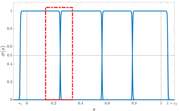
Figure 3: Example of double sigmoid functions $\sigma_{k}(s)$ for the set of five waypoints shown in Figure 2. The use of $\epsilon_{1}$ and $\epsilon_{2}$ the way described in (8) leads to $\sigma_{1}^{r}(-\epsilon_{1})=0.5$ and $\sigma_{n_{w}}^{f}(1+\epsilon_{2})=0.5$, thus ensuring that $\sigma_{1}(0)=1$ and $\sigma_{n_{w}-1}(1)=1$. The red rectangle highlights a transition region, and it can be shown that the sum of the two sigmoids involved in this transition is equal to one.

We note that the larger the value of $\beta$ in (8) is the more closely the smooth path described by (6) follows the piecewise linear path between waypoints in $\mathcal{W}$. Figure 4 shows examples of paths at different values of $\beta$ for the same path depicted in Figure 2.

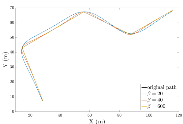
Figure 4: Demonstration of the effect of changing the value of $\beta$ in (8) on how closely (6) follows the original piecewise linear path.

Lemma 1.

For a path described by $p(s)$ in (6), with the double sigmoid functions as described in (8) and provided that $\beta\gg 1$ then the following statement holds

$$\sum_{i=1}^{n_{w}-1}\Sigma_{i}(s)\bar{w}_{i}(s)\approx 0$$

where $\Sigma_{i}(s)=\beta\sigma_{i}(s)(\sigma_{i}^{f}(s)-\sigma_{i}^{r}(s))$

Proof.

At a waypoint $w_{i}$ we consider the two functions $\Sigma_{i-1}(s)$ and $\Sigma_{i}(s)$ (both involve $s=s_{i}$ in their definition) and we note that the values of other $\Sigma$ are equal to zero by definition. We want to evaluate $D=\Sigma_{i-1}(s)\bar{w}_{i-1}+\Sigma_{i}(s)\bar{w}_{i}$ but we do so within a band $\delta_{s}$ around $s_{i}$, i.e. at $s^{\prime}=s+\delta_{s}$

$$\begin{split}D&=\beta\sigma_{i-1}(s_{i}+\delta_{s})(\sigma_{i-1}^{f}(s^{\prime})-\sigma_{i-1}^{r}(s^{\prime}))\bar{w}_{i-1}(s^{\prime})\\ &+\beta\sigma_{i}(s_{i}+\delta_{s})(\sigma_{i-1}^{f}(s^{\prime})-\sigma_{i}^{r}(s^{\prime}))\bar{w}_{i}(s^{\prime})\end{split}$$ (11)

then substituting $\beta\gg 1$ in the last equation we get the following

$$D=\frac{\beta\delta_{s}e^{-\beta\delta_{s}}}{\left(1+e^{-\beta\delta_{s}}\right)^{2}}\left(\frac{w_{i-1}}{s_{i}-s_{i-1}}+\frac{w_{i+1}}{s_{i+1}-s_{i}}\right)$$ (12)

If $\delta_{s}=0$ in (12) then $D=0$, and otherwise the quotient $\tfrac{\beta e^{\beta\delta_{s}}}{\left(1+e^{\beta\delta_{s}}\right)^{2}}$ can be made arbitrarily small by choosing large $\beta$. We also note that $\tfrac{\beta e^{\beta\delta_{s}}}{\left(1+e^{\beta\delta_{s}}\right)^{2}}=\tfrac{\beta e^{-\beta\delta_{s}}}{\left(1+e^{-\beta\delta_{s}}\right)^{2}}$ meaning the same result follows for $\delta_{s}>0$ and $\delta_{s}<0$. The statement of the lemma follows by applying the same summation for all values of $i$. ∎

4.2 Energy sufficiency

We consider the case in which the robot lies at the beginning of the smooth path (6) and moves along this path back to the station (at the other end of the path). We assume the path is static, i.e. not changing.

We define a reference point along the path as in (6)

$$\begin{split}x_{r}(s)&=p(s)=\sum_{i=1}^{n_{w}-1}\sigma_{i}(s)\left(\tfrac{s_{i+1}-s}{s_{i+1}-s_{i}}w_{i}+\tfrac{s-s_{i}}{s_{i+1}-s_{i}}w_{i+1}\right)\\ \frac{\partial x_{r}}{\partial s}&=\sum_{i=1}^{n_{w}-1}\sigma_{i}(s)\frac{w_{i+1}-w_{i}}{s_{i+1}-s_{i}}\end{split}$$ (13)

noting that the derivative expression follows from Lemma 1. We want to control the value of $s$ in a way that makes the reference point approach the end of path in a manner commensurate to the robot’s energy content. For this purpose, we introduce the following dynamics for $s$

$$\dot{s}=\eta$$ (14)

with $\eta\in\mathbb{R}$ and $s(0)=0$. The outline of our strategy is as follows: we introduce constraints that manipulate the value of $s$ in a way that makes the reference point $x_{r}$ approach the end of path as the total energy content decreases, and use an additional constraint to make the robot follow $x_{r}$. The candidate CBF for energy sufficiency is

$$h_{e}=E_{nom}-E-\tfrac{\mathcal{P}(v_{r})}{v_{r}}(L(1-s)-\delta)$$ (15)

where $v_{r}$ is the desired velocity with which the robot moves along the path, $\delta$ is the distance of the boundary of charging region away from its center, noting that the center of the charging region is $w_{n_{w}}$. We note is the expression $L(1-s)$ expresses the length along the path from point $x_{r}(s)$ till its end. The constraint $\dot{h}_{e}\geq-\alpha(h_{e})$ associated with this candidate CBF is

$$\begin{split}&-\mathcal{P}(u)+\tfrac{\mathcal{P}(v_{r})}{v_{r}}L\eta\geq-\gamma_{e}h_{e}\end{split}$$ (16)

In (15) the value of $s$ needs to be maintained above zero (otherwise the value of $h_{e}$ can be still positive without having the reference point $x_{r}$ moving back towards the end of the path). For this end we introduce a constraint that lower bounds $s$ with the following candidate CBF

$$h_{b}=s$$ (17)

with the associated constraint

$$\eta\geq-\gamma_{b}h_{b}$$ (18)

We complement (15) and (17) with another candidate CBF that aims at making the robot follow $x_{r}(s)$ as it changes, and is defined as follows

$$h_{d}=\tfrac{1}{2}(d^{2}-||x-x_{r}(s)||^{2})$$ (19)

with $0<d<\delta$. The constraint associated with this candidate CBF is

$$-(x-x_{r}(s))^{T}(u-\dot{x}_{r}(s))\geq-\gamma_{d}h_{d}$$ (20)

where $\dot{x}_{r}=\tfrac{\partial x_{r}}{\partial s}\eta$.

In the following lemmas we show that the proposed CBFs lead the robot back to the charging station with $E_{nom}-E\geq 0$. We note that we are not controlling $u$ in (16) but rather give this task to (20), thus partially decoupling the reference point’s movement from the robot’s control action. In other words, we deliberately make the system respond to changing energy levels by moving the reference point along the path without directly changing the robot’s velocity. This interplay between energy sufficiency and tracking constraints is highlighted in the next lemma.

Lemma 2.

For a robot with dynamics described in (4) and power consumption as in (5), and has a maximum magnitude of control action $u_{\text{max}}$, the control barrier functions defined in (15) and (19) are zeroing control barrier functions (ZCBF) provided that

$$v_{r}^{*}=\sqrt{\frac{m_{0}}{m_{2}}}\leq u_{\text{max}}$$

where $||u||\leq u_{max}$. Moreover, provided that $L(s)>\delta$, then $E=E_{nom}$ only at $L(1-s)=\delta$.

Proof.

The idea of the proof is to show that there is always a value of $\eta$ that satisfies (16) with its $\mathcal{P}(u)$ term, and there is always $u$ to satisfy (20) at the same time. Since $\eta\in\mathbb{R}$ means there is always a value of $\eta$ that satisfies (16), thus (15) is a ZCBF. However, the reference point $x_{r}$ could be moving with a speed too fast for the robot to track depending on the value of $\mathcal{P}(u)$.

We consider the critical case of approaching the boundary of the safe set for both $h_{d}$ and $h_{e}$, i.e. $h_{e}\approx 0$ and $h_{d}\approx 0$, in which case we can consider the equality condition of the constraints (16) and (20) (i.e. near the boundary of the safe set the safe actions should at least satisfy $\dot{h}=-\alpha h$ for both (16) and (20)). The aforementioned constraints become

$$\eta=\frac{\mathcal{P}(u)}{\mathcal{P}(v_{r})}\frac{v_{r}}{L}$$ (21a)

$$u=\frac{\partial x_{r}}{\partial s}\eta=\frac{\partial x_{r}}{\partial s}\frac{\mathcal{P}(u)}{\mathcal{P}(v_{r})}\frac{v_{r}}{L}$$ (21b)

noting that $x-x_{r}\neq 0$ when $h_{d}\approx 0$. We also note that

$$||u||=\frac{\mathcal{P}(u)}{\mathcal{P}(v_{r})}\frac{v_{r}}{L}\left\lVert\frac{\partial x_{r}}{\partial s}\right\rVert.$$

Assuming $\beta\gg 1$, the derivative $\tfrac{\partial x_{r}}{\partial s}$ is as described in (6). Moreover,

$$s_{i+1}-s_{i}=\frac{\sum_{k=1}^{i}\ell_{k}-\sum_{k=1}^{i-1}\ell_{k}}{L}=\frac{||w_{i+1}-w_{i}||}{L}$$ (22)

where $\ell_{k}=||w_{k+1}-w_{k}||$ and consequently $\tfrac{\partial x_{r}}{\partial s}$ can be expressed as

$$\tfrac{\partial x_{r}}{\partial s}=L\sum_{i=1}^{n_{w}-1}\sigma_{i}(s)\hat{e}_{i}$$ (23)

where $\hat{e}_{i}=\tfrac{w_{i+1}-w_{i}}{||w_{i+1}-w_{i}||}$ is a unit vector. To estimate $\left\lVert\tfrac{\partial x_{r}}{\partial s}\right\rVert$ it suffices to mention that in the range $s_{i}+\epsilon_{m}<s<s_{i+1}-\epsilon_{m}$ (for $i=1,\dots,n_{w}-1$ and $\epsilon_{m}=\tfrac{2}{\beta}$) all the double sigmoid functions in (23) will be almost equal to zero except for one (by definition) and thus $\left\lVert\tfrac{\partial x_{r}}{\partial s}\right\rVert=L$. Moreover, if $s_{i}-\epsilon_{m}<s<s_{i}+\epsilon_{m}$, i.e. $s$ is transitioning from one segment to the next, the sum of the two sigmoid functions locally around $s=s_{i}$ is equal to one as show in (9), meaning that (23) will be a convex sum of two unit vectors which will have at most a magnitude equal to one so $\left\lVert\tfrac{\partial x_{r}}{\partial s}\right\rVert\leq L$. Therefore $||u||$ becomes

$$||u||=\frac{\mathcal{P}(u)}{\mathcal{P}(v_{r})}v_{r}$$ (24)

which is a root finding problem for a polynomial of the second degree, since $\mathcal{P}(u)$ is a second order polynomial (5). Solving for the roots we get

$$\lambda_{1}=v_{r},\quad\lambda_{2}=\frac{m_{0}}{m_{2}v_{r}}$$ (25)

and these roots are equal when $v_{r}^{*}=\sqrt{\tfrac{m_{0}}{m_{2}}}$. Since we consider a case where the robot is stationary and the path is fixed, the robot starts from this stationary state and converges to $||u||=\min(\lambda_{1},\lambda_{2})$ for a given value of $v_{r}$. This means that the maximum achievable return velocity is at $v_{r}=v_{r}^{*}$ where $\lambda_{1}=\lambda_{2}$. If $v_{r}^{*}\leq u_{max}$ then there is always a control action $u$ available to satisfy (20), rendering (19) a ZCBF. If $h_{e}=0$ then from (15) $E=E_{nom}$ can only happen if $L(1-s)=\delta$, meaning the remaining length along the path is equal to delta, which only happens at the boundary of the charging region. ∎

Remark 1.

The previous proof assumes the presence of a-priori known model for power consumption. However, a mismatch between the power model $\mathcal{P}(u)$ in (5) and the actual power consumption $\bar{\mathcal{P}}(u)$ will lead to a different solution of (24). We are interested in the case where $\bar{\mathcal{P}}(u)=\mathcal{P}(u)+\Delta_{p}$, with $\Delta_{p}\in\mathbb{R}$. The root finding problem in (24) becomes

$$||u||=\frac{\bar{\mathcal{P}}(u)}{\mathcal{P}(v_{r})}v_{r}$$ (26)

and the roots will be

$$\bar{\lambda}_{1,2}=\frac{m_{0}+m_{2}v_{r}^{2}\pm\mathcal{D}}{2m_{2}v_{r}}$$ (27)

where $\mathcal{D}=\sqrt{(m_{0}-m_{2}v_{r}^{2})^{2}-4m_{2}v_{r}^{2}\Delta_{p}}$. When $\Delta_{p}=0$, $\bar{\lambda}_{1,2}=\lambda_{1,2}$ as described in (25). If $\Delta_{p}>0$, then $\mathcal{D}<(m_{0}-m_{2}v_{r}^{2})$ and as a result $\bar{\lambda}_{1}>v_{r}$ and $\bar{\lambda}_{2}<\tfrac{m_{0}}{m_{2}v_{r}}$. In other words, the robot will converge to a faster speed in case the actual power consumption is more than expected, and the converse is true for $\Delta_{p}<0$. When

$$\Delta_{p}>\Delta_{p}^{*}=\left(\tfrac{m_{0}-m_{2}v_{r}^{2}}{2v_{r}\sqrt{m_{2}}}\right)^{2}$$ (28)

$\mathcal{D}$ becomes undefined and there will be no roots for (26), indicating a point of instability in velocity for power disturbances beyond $\Delta_{p}^{*}$. This idea is illustrated in Figure 5.

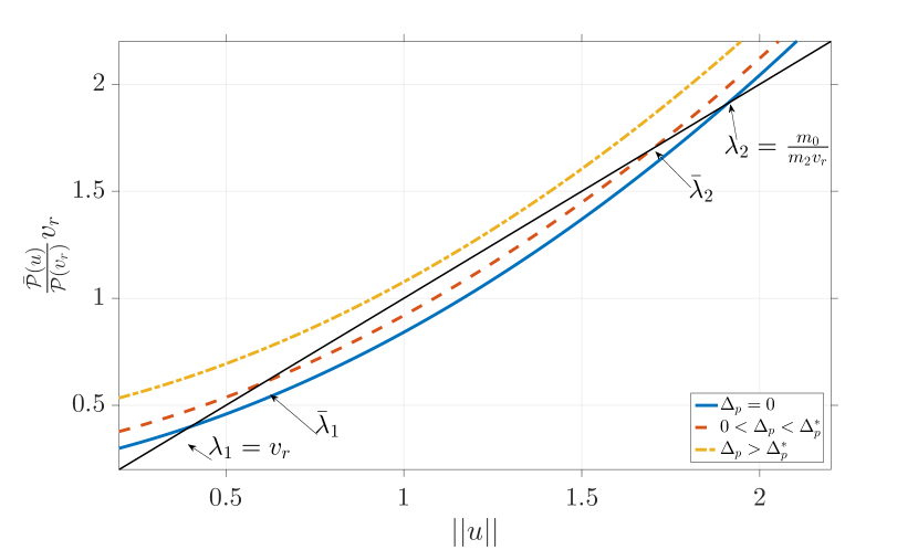
Figure 5: Graphical representation for the roots of (26) for different values of disturbance power $\Delta_{p}$. The roots are intersections of the straight line $f_{1}(u)=||u||$ in black and the parabolas $f_{2}(u)=\tfrac{\bar{\mathcal{P}}(u)}{\mathcal{P}(v_{r})}v_{r}$ (representing RHS and LHS of (26) respectively).

Lemma 3.

For a robot with dynamics (4), the candidate CBF (17) is a ZCBF.

Proof.

Since $\eta\in\mathbb{R}$ then there exist a value of $\eta$ that satisfies (18). We need to show that this constraint does not conflict with (16) when both constraints are on the boundary of their respective safe sets, i.e. $h_{e}=h_{b}=0$. From (16)

$$\eta\geq\frac{\mathcal{P}(u)}{\bar{\mathcal{P}}(v_{r})}\frac{v_{r}}{L}$$ (29)

while (18) becomes $\eta\geq 0$. Since the right hand side of (29) is always positive, it means there is always a value of $\eta$ that satisfies both (29) and (18), thus (17) is a ZCBF. ∎

Although from Lemma 2 we show that $E(t)=E_{nom}$ on the boundary of the charging region, this is a result that concerns the reference point’s position $x_{r}$ while the robot’s actual position tracks $x_{r}$ through enforcing the constraint (19). This situation implies the possibility of $x_{r}$ reaching a point where $L(s)=\delta$ (boundary of charging region) while the robot’s position is lagging behind. In other words, we need the instant where $E(t)=E_{nom}$ to happen inside of the charging region or at least on its boundary.

Proposition 1.

Consider a robot with dynamics (4) and applying the constraints pertaining to the CBFs (15), (17) and (19). We define a modified distance threshold $\delta_{m}$ as

$$\delta_{m}\leq\delta-d$$ (30)

then using $\delta_{m}$ in (15) ensures that $E(t)$ will be at most equal to $E_{nom}$.

Proof.

Figure 6: Demonstration of $x_{r}$ pursuing $\delta_{m}$ as the boundary of the charging region in (15) while having a robot following the reference point $x_{r}$ at a distance $d$ away. Here $x_{r}$ is the reference point position, $x_{c}$ is the charging station center position, $\delta$ is the charging region’s radius, and $\delta_{m}$ is a reduced radius to track as described in (30).

From Lemma 2 $E=E_{nom}$ only at $L(1-s)=\delta_{m}$, which is equal to the length of $(x_{c},x_{r})$ segment in Figure 6, i.e. the remaining length along the path from $x_{r}$ to $x_{c}$. This implies that $||x-x_{c}||\leq\delta$ as demonstrated in Figure 6.

∎

Theorem 1.

For a robot with dynamics described by (4) and maximum magnitude of control action $u_{max}$, applying the QP in (3) with constraints (16) (with $\delta=\delta_{m}$ from (30)), (20) and (18), and with a static piecewise linear path with waypoints $\mathcal{W}$, then energy sufficiency is maintained , i.e. $E<E_{nom}$ if $||x-x_{c}||>\delta$.

Proof.

If we substitute $\delta_{m}$ from (30) in (15) and (16), then from lemma 2 $E=E_{nom}$ iff $L(1-s)=\delta_{m}$, and from proposition 1 this implies that $||x-x_{c}||<\delta$ when $E=E_{nom}$, and since $E$ is strictly increasing (due to $\mathcal{P}(u)>0$ by definition), we conclude that $E\leq E_{nom}$ in $||x-x_{c}||>\delta$. ∎

5 Energy sufficiency over a dynamic path

We extend the results from the previous section to consider the case in which the path is changing with time due to robot’s movement and replanning actions.

5.1 Effect of robot’s movement

Assuming that the path is fixed (i.e., there is no replanning), the main difference from the static case is that the first waypoint $w_{1}\in\mathcal{W}$ is the robot’s position, leading to a change in the total path length $L$ as the robot moves. Additionally, the values of $s_{i}$ at the different waypoints will change as a result. We therefore consider the following simple proportional control dynamics for $w_{1}$:

$$\dot{w}_{1}=\xi=-k_{w}(w_{1}-x)$$ (31)

where $K_{w}\gg 0$ and $\xi\in\mathbb{R}$. The change in total path length is:

$$\begin{split}\dot{L}&=\frac{d}{dt}\left(\sum_{i=2}^{n_{w}-1}||w_{i+1}-w_{i}||+||w_{2}-w_{i}||\right)\\ &=-\frac{(w_{2}-w_{1})}{||w_{2}-w_{1}||}\xi,\end{split}$$ (32)

noting that all the waypoints other than $w_{1}$ are fixed. The change in $s_{i}$ is

$$\dot{s}_{i}=\frac{d}{dt}\frac{L_{i}}{L}=\frac{d}{dt}\left(1-\frac{\bar{L}_{i}}{L}\right)=\frac{\bar{L}_{i}}{L^{2}}\dot{L}$$ (33)

where $\bar{L}_{i}$ is the length along the path from waypoint $w_{i}$ to the end of the path and is constant for $i=2,\dots,n_{w}-1$. The derivative $\tfrac{dx_{r}}{dt}$ is:

$$\frac{dx_{r}}{dt}=\frac{\partial x_{r}}{\partial s}\eta+\frac{\partial x_{r}}{\partial t}$$ (34)

where $\tfrac{\partial x_{r}}{\partial t}$ follows from differentiating (6) with respect to time:

$$\frac{\partial x_{r}}{\partial t}=\sum_{i=1}^{n_{w}-1}\sigma_{i}(s)\left(w_{i+1}-w_{i}\right)\tfrac{\dot{L}}{L^{2}}\tfrac{\bar{L}_{i}(s_{i+1}-s)+\bar{L}_{i+1}(s-s_{i})}{(s_{i+1}-s_{i})^{2}}.$$ (35)

Consequently, the energy sufficiency constraint (16) becomes

$$\begin{split}&-\mathcal{P}(u)+\tfrac{\bar{\mathcal{P}}(v_{r})}{v_{r}}(L\eta-\dot{L}(1-s))\geq-\gamma_{e}h_{e}\end{split}$$ (36)

and the tracking constraint (20) now uses $\dot{x}_{r}$ as in (34).

The results from Theorem 1 rely on the fact that the path is static. To use the same result in the dynamic case we “freeze” the path when the robot needs to go back to recharge, i.e. we stop $w_{1}$ from tracking robot’s position when it needs to go back to recharge:

Proposition 2.

Consider a robot with dynamics (4) applying the proposed energy sufficiency framework described by the CBFs (15) and (17). Consider the following dynamics for $w_{1}$

$$\dot{w}_{1}=\xi=-k_{w}(w_{1}-x)\left(1-\zeta(s)\right)$$ (37)

where $\zeta$ is an activation function defined as

$$\zeta(s)=\begin{cases}0\quad s\leq\epsilon_{a}\\ 1\quad\text{otherwise}\end{cases}$$ (38)

with $0<\epsilon_{a}\ll\bar{\epsilon}_{a}<1$ and $||w_{1}-x_{r}(\bar{\epsilon}_{a})||=d$, then (15) and (19) are ZCBF.

Proof.

We start by noting that (37) achieves tracking of the robot’s position in case $s=0$, with an error inversely proportional to $k_{w}$, according to the candidate Lyapunov function

$$\scriptsize V=\tfrac{1}{2}(x-w_{1})^{T}(x-w_{1}),\quad\dot{V}=(x-w_{1})^{T}u-k_{w}||x-w_{1}||^{2}$$ (39)

which has $\dot{V}\leq 0$ under high value of $k_{\omega}$ (which is feasible since $\xi$ is an imaginary point with no physical characteristics). Moreover, since $\eta\in\mathbb{R}$ then there is a value of $\eta$ capable of satisfying the following inequality

$$\begin{split}&\eta\geq\frac{1}{L}\left(\tfrac{\mathcal{P}(u)-\gamma_{e}h_{e}}{\mathcal{P}(v_{r})}v_{r}+\dot{L}(1-s)\right).\end{split}$$ (40)

We need to show that if $0<s<\epsilon_{a}$ (when the reference point starts moving but the path freezing has not been activated yet, according to (38)), tracking and energy sufficiency constraints are not violated as well as that $s$ increases so that $s>\epsilon_{a}$.

To prove the latter, we need to show that the right hand side of (40) is positive when $h_{e}\approx 0$, i.e. near the boundary of energy sufficiency safe set. The term $\tfrac{\mathcal{P}(u)}{\mathcal{P}(v_{r})}v_{r}>0$ by definition, so the sign of the right hand side of (40) depends on sign of $\dot{L}$. It can be shown that the sign of $\dot{L}(1-s)$ depends on the sign of $\tfrac{d}{dt}||w_{1}-w_{2}||$, therefore even if $\tfrac{d}{dt}||w_{1}-w_{2}||<0$, it will be so until $||w_{1}-w_{2}||\approx 0$, when the right hand side of (40) will be positive. Therefore, when $h_{e}\approx 0$, $\eta>0$, meaning $s$ will increase even when $0<s<\epsilon_{a}$.

As a result, the reference point $x_{r}$ moves along the path and $h_{d}$ in (19) approaches zero (in the limit case $||w_{1}-x_{r}||=d$ at $s=\bar{\epsilon}_{a}$). The fact that $s(t)$ is continuous and $\epsilon_{a}\ll\bar{\epsilon}_{a}$ implies that $\dot{w}_{1}=0$ before $s(t)=\bar{\epsilon}_{a}$, i.e. the path freezes while $h_{d}>0$, so the path freezing condition (38) does not violate the tracking CBF $h_{d}$, nor the energy sufficiency CBF $h_{e}$, and consequently the result of lemma 2 follows (since $h_{e}\approx 0$ and $\eta>0$ implying $s>0$ leading to $h_{d}\approx 0$).

∎

The full QP problem with the constraints discussed so far can be expressed as

$$\mathbf{u}^{*}=\underset{\mathbf{u}}{\text{min}} ||\mathbf{u}-\mathbf{u}_{nom}||^{2}$$ (41)

         s.t. $$\mathbf{A}\mathbf{u}\geq\mathbf{B}$$

where

$$\begin{split}\mathbf{A}&=\begin{bmatrix}\tfrac{\mathcal{P}(v_{r})}{v_{r}}L&\mathbf{0}_{1\times 2}\\ 1&\mathbf{0}_{1\times 2}\\ (x-x_{r})^{T}\tfrac{\partial x_{r}}{\partial s}&-(x-x_{r})^{T}\end{bmatrix}\\ \mathbf{B}&=\begin{bmatrix}-\gamma_{e}h_{e}+\mathcal{P}(u)+\dot{L}(1-s)\\ -\gamma_{b}h_{b}\\ -\gamma_{d}h_{d}\end{bmatrix}\\ \mathbf{u}_{nom}&=\begin{bmatrix}0&u_{nom}\end{bmatrix}\end{split}$$ (42)

Theorem 2.

For a robot described by (4) with a set of ordered waypoints $\mathcal{W}\in\mathbb{R}^{n_{w}\times 2}$, (41) ensures energy sufficiency.

Proof.

Since (15) and (19) are valid ZCBFs from Proposition 2 and (17) is a valid ZCBF then from Lemma 3, then from Proposition 1 and Lemma 2 (augmented by Proposition 2) $E(t)=E_{nom}$ at $||x-x_{c}||<\delta$ (inside the charging region), and since $E(t)$ is strictly increasing it means $E(t)<E_{nom}$ for $||x-x_{c}||>\delta$, as shown by Theorem 1, i.e. energy sufficiency is maintained. ∎

5.2 Effect of path planning

During the course of a mission, the path planner keeps updating the waypoints back to the charging station every $\mathcal{T}$ seconds, meaning that there are discrete changes in the number of waypoints and their locations, which can lead to violating the energy sufficiency constraint. To account for these changes, we impose some conditions on the output of the path planner so as not to violate other constraints.

Definition 2.

Assuming there is a path $\mathcal{W}^{(k-1)\mathcal{T}}=\{w_{1}^{(k-1)\mathcal{T}},\dots,w_{n_{w}}^{(k-1)\mathcal{T}}\}$ at time $(k-1)\mathcal{T}$ between a robot at position $x(k\mathcal{T})=w_{1}^{(k-1)\mathcal{T}}$ and the charging station, Sequential Path Construction (SPC) is the process of creating a new set of waypoints $\mathcal{W}^{k\mathcal{T}}=\{w_{1}^{k\mathcal{T}},\dots,w_{n_{w}+1}^{k\mathcal{T}}\}$ at time $k\mathcal{T}$ provided that $\zeta(s)=0$, where $\zeta(s)$ is defined in (38), such that

$$\begin{split}w_{1}^{k\mathcal{T}}&=x(k\mathcal{T})\\ w_{2}^{k\mathcal{T}}&=\kappa w_{1}^{k\mathcal{T}}+(1-\kappa)w_{3}^{k\mathcal{T}}\\ w_{i+1}^{k\mathcal{T}}&=w_{i}^{(k-1)\mathcal{T}},\quad i=2,\dots,n_{w}\end{split}$$ (43)

where $0\ll\kappa<1$.

Lemma 4.

Sequential Path Construction is path length and path angle invariant, meaning the following two equations are satisfied

$$\begin{split}\sum_{i=1}^{n_{w}-1}||w_{i}^{(k-1)\mathcal{T}}-w_{i+1}^{(k-1)\mathcal{T}}||&=\sum_{i=1}^{n_{w}}||w_{i}^{k\mathcal{T}}-w_{i+1}^{k\mathcal{T}}||\\ \sum_{i=2}^{n_{w}-1}|\psi_{i}^{(k-1)\mathcal{T}}|&=\sum_{i=2}^{n_{w}}|\psi_{i}^{k\mathcal{T}}|\end{split}$$ (44)

where

$$\psi_{i}=\cos^{-1}\frac{\Delta w_{i-1}^{i}.\Delta w_{i}^{i+1}}{||\Delta w_{i-1}^{i}||.||\Delta w_{i}^{i+1}||}$$ (45)

and $\Delta w_{i}^{i+1}=w_{i+1}-w_{i}$

Proof.

The path length at time $k\mathcal{T}$ is

$$\begin{split}&L^{k\mathcal{T}}=\sum_{i=1}^{n_{w}}||w_{i}^{k\mathcal{T}}-w_{i+1}^{k\mathcal{T}}||\\ &=||w_{1}^{k\mathcal{T}}-w_{2}^{k\mathcal{T}}||+||w_{2}^{k\mathcal{T}}-w_{3}^{k\mathcal{T}}||+\sum_{i=3}^{n_{w}}||w_{i}^{k\mathcal{T}}-w_{i+1}^{k\mathcal{T}}||\\ &=||w_{1}^{k\mathcal{T}}-w_{3}^{k\mathcal{T}}||+\sum_{i=2}^{n_{w}}||w_{i}^{(k-1)\mathcal{T}}-w_{i+1}^{(k-1)\mathcal{T}}||\\ &=||w_{1}^{(k-1)\mathcal{T}}-w_{2}^{(k-1)\mathcal{T}}||+\sum_{i=2}^{n_{w}}||w_{i}^{(k-1)\mathcal{T}}-w_{i+1}^{(k-1)\mathcal{T}}||\\ &=L^{(k-1)\mathcal{T}}.\end{split}$$ (46)

By definition we have: $\psi^{(k-1)\mathcal{T}}_{i}=\psi^{k\mathcal{T}}_{i+1}$ for $i=2,\dots,n_{w}$. Since $w_{3}^{k\mathcal{T}}-w_{2}^{k\mathcal{T}}=(1-\kappa)(w_{3}^{k\mathcal{T}}-w_{1}^{k\mathcal{T}})$ and $w_{2}^{k\mathcal{T}}-w_{1}^{k\mathcal{T}}=\kappa(w_{3}^{k\mathcal{T}}-w_{1}^{k\mathcal{T}})$, then $\cos\psi_{2}^{k\mathcal{T}}=1$ therefore $\psi_{2}^{k\mathcal{T}}=0$. In conclusion $\sum_{i=2}^{n_{w}-1}|\psi_{i}^{(k-1)\mathcal{T}}|=\sum_{i=2}^{n_{w}}|\psi_{i}^{k\mathcal{T}}|$. ∎

Proposition 3.

Sequential Path Construction does not violate energy sufficiency, provided $\mathbf{u}_{nom}$ is Lipschitz.

Proof.

We need to show that changing the path with SPC does not affect the following two inequalities if they are satisfied for the original path:

$$h_{e}=E_{nom}-E-\tfrac{\mathcal{P}(v_{r})}{v_{r}}(L(1-s)-\delta_{m})\geq 0$$ (47a)

$$-\mathcal{P}(u_{nom})+\tfrac{\mathcal{P}(v_{r})}{v_{r}}\left(L\eta_{nom}-\dot{L}(1-s)\right)\geq-\gamma_{e}h_{e}$$ (47b)

Since $\eta_{nom}$ and $u_{nom}$ are continuous, then $\mathcal{P}(u_{nom}),E$ and $s$ are all continuous with no jumps (i.e., discrete changes). Since path length is invariant under SPC by virtue of Lemma 4, then $L$ in (47b) does not change as well as $\dot{L}$, meaning that (47b) is not violated under SPC. ∎

Based on the proposition above, we introduce the Algorithm 1 that admits new paths produced by the path planner as long as they do not violate (47b), and otherwise switches to SPC.

Algorithm 1 Admission of new path at time $k\mathcal{T}$

$\mathcal{W}^{(k-1)\mathcal{T}}$,$\mathcal{W}^{k\mathcal{T}}_{candidate}$, $x$,$\mathbf{u}_{nom}$

$L,h_{e}\leftarrow$ EVALUATE_PATH($\mathcal{W}^{k\mathcal{T}}_{candidate},\mathbf{u}_{nom}$)

if $\zeta(s)==0$ then

     if (47a) == False OR (47b) == False then

         $\mathcal{W}^{k\mathcal{T}}\leftarrow$ SPC_PATH$(x(k\mathcal{T}),\mathcal{W}^{(k-1)\mathcal{T}})$

     else

         $\mathcal{W}^{k\mathcal{T}}\leftarrow\mathcal{W}^{k\mathcal{T}}_{candidate}$

     end if

end if

return $\mathcal{W}^{k\mathcal{T}}$

In Algorithm 1, EVALUATE_PATH($\mathcal{W}^{k\mathcal{T}},\mathbf{u}_{nom}$) is a function that takes the candidate path points from the path planner and evaluates the path length, as well as the value of $h_{e}$, and SPC_PATH$(x(k\mathcal{T}),\mathcal{W}^{(k-1)\mathcal{T}})$ is a function that updates a path using SPC.

Theorem 3.

For a robot described by (4) that applies the control strategy in (41) for an already existing set of waypoints $\mathcal{W}^{(k-1)\mathcal{T}}$ at time $(k-1)\mathcal{T}$, $k\in\mathbb{N}$. Suppose a path planner produces a candidate set of waypoints $\mathcal{W}^{k\mathcal{T}}$ at time $k\mathcal{T}$ that satisfies the conditions in (47b) and provided that $\zeta(s)=0$ from (38), then Algorithm 1 ensures energy sufficiency is maintained.

Proof.

If the new set of augmented waypoints satisfies (47a), then switching from $\mathcal{W}^{(k-1)\mathcal{T}}$ to $\mathcal{W}^{k\mathcal{T}}$ does not violate the energy sufficiency constraint encoded by $h_{e}$. Moreover, if said switching satisfies (47b), then $h_{e}>0$ is satisfied with $\eta_{nom}$ at $s=0$, meaning that $w_{1}$ tracks $x$ as outlined in Proposition 2 and consequently $x_{r}$ tracks the robot’s position (since $s=0$ and $w_{1}$ tracks robot’s position), thus $h_{d}>0$ is not violated as well, which means the sufficiency and tracking constraints are not violated by the path update.

When $s>0$, i.e. $\zeta(s)\neq 0$, the path is frozen and energy sufficiency is maintained by virtue of Theorem 2. If either condition in (47b) is violated, the path is updated using SPC which maintains energy sufficiency as discussed in Proposition 3. Therefore Algorithm 1 ensures energy sufficiency and tracking constraints are not violated.

∎

6 Application to unicycle-type robots

The method described so far uses a single integrator model to describe robot dynamics. Although such model choice is widely used in robotics and has the advantage of versatility (Zhao and Sun, 2017), applying it directly to more specific robot models needs proper adaptation, especially considering the effects of unmodelled modes of motion on power consumption. In this section we describe a method to apply the proposed framework on a non-holonomic wheeled robot, which has the added characteristic of being able to spin. More specifically we are interested in robots with the following unicycle kinematic model

$$\begin{split}\dot{x}_{1}&=v\cos\theta\\ \dot{x}_{2}&=v\sin\theta\\ \dot{\theta}&=\omega\end{split}$$ (48)

where $x=\begin{bmatrix}x_{1}x_{2}\end{bmatrix}^{T}\in\mathbb{R}^{2}$ is robot’s position, $\theta\in\mathbb{R}$ is its orientation, $v\in\mathbb{R}$ and $\omega\in\mathbb{R}$ are the linear and angular speeds respectively which act as inputs. A single integrator speed $u$ from (41) can be transformed to linear and angular speeds for a unicycle through the following relation (Ogren et al., 2001):

$$\begin{bmatrix}v\\ \omega\end{bmatrix}=\begin{bmatrix}1&0\\ 0&\tfrac{1}{\ell}\end{bmatrix}\begin{bmatrix}\cos\theta&\sin\theta\\ -\sin\theta&\cos\theta\end{bmatrix}u$$ (49)

where $\ell>0$ is a distance from the robot’s center to an imaginary handle point. We also choose to be able to move backward when the value of $v$ becomes negative by doing the following

$$\begin{split}v^{\prime}&=v\\ \omega^{\prime}&=\omega\frac{v}{|v|}\end{split}$$ (50)

A robot described by (49) consumes additional power due to its angular speed $\omega$ in addition to what is consumed by its linear speed $v$, which calls for augmenting (5) with additional terms

$$\begin{split}\mathcal{P}_{u}(v,\omega)&=m_{u_{0}}+m_{u_{1}}|v|+m_{u_{2}}|v|^{2}+m_{u_{1}}^{\prime}|\omega|+m_{u_{2}}^{\prime}|\omega|^{2}\\ \end{split}$$ (51)

We note that in this power model we assume no direct coupling effects between linear and angular speeds on power consumption.

Remark 2.

The power model in (51) is different from that in (5) and we seek to establish a relation between the two. When a robot is moving in a straight line, then $\mathcal{P}_{u}(v,0)=\mathcal{P}(u)$. From (49) $||u||=\sqrt{v^{2}+(\omega\ell)^{2}}$ so when $\omega\neq 0$, $v$ decreases for the same $||u||$, meaning $\mathcal{P}_{u}(v,0)\leq\mathcal{P}_{u}(v,\omega)$. In this case we either have $\mathcal{P}(u)>\mathcal{P}_{u}(v,\omega)$ meaning that turning has no contribution to power consumption, or $\mathcal{P}(u)\leq\mathcal{P}_{u}(v,\omega)$ which means turning has significant contribution in power consumption. We are interested in the latter case and we consider that

$$\mathcal{P}_{u}(v,\omega)\leq\mathcal{P}(u)+\Delta_{\omega}$$ (52)

where $\Delta_{\omega}\in\mathbb{R}$ is the change in power due to rotation.

Using a power model that only accounts for linear speed is akin to having the power consumption due to $\omega$ as a disturbance power $\Delta_{\omega}$, which may lead to instability as discussed in Remark 1. A solution to this issue is choosing a fairly slow return speed value $v_{r}$ so as to increase the stability margin $\Delta_{p}^{*}$ in (28), however this may impose undesirable limitations on performance.

Since the path we are using is essentially a piecewise linear path with waypoints $w_{i},i=1,\dots,n_{w}$, robot spinning will be mostly near these waypoints when it is changing its direction of motion. The idea behind our proposed adaptation is to add a certain amount of power $\tilde{\delta}$ to $\mathcal{P}(v_{r})$ in (26) near the path’s waypoints so that roots of (26) always exist. In other words, if we define $\tilde{\mathcal{P}}(v_{r})=\mathcal{P}(v_{r})+\tilde{\delta}$, we ensure that roots for the following equation always exist

$$||u||=\frac{\bar{\mathcal{P}}(u)}{\tilde{\mathcal{P}}(v_{r})}v_{r}=\frac{\mathcal{P}(u)+\Delta_{\omega}}{\mathcal{P}(v_{r})+\tilde{\delta}}v_{r}$$ (53)

We note that choosing $\tilde{\delta}>\Delta_{\omega}$ has the effect of slowing down the robot (since $\bar{\mathcal{P}}(u)-\tilde{\mathcal{P}}(u)<0$, we have a similar effect of having a negative disturbance power $\Delta_{p}$ in (26), which slows down the robot as discussed in Remark 1). Therefore, choosing a constant value for $\tilde{\delta}$ such that $\tilde{\delta}>\Delta_{\omega}$ is equivalent to choosing a lower value of $v_{r}$.

Instead of using a constant value for $\tilde{\delta}$, our approach is to use double sigmoid functions to make the value of $\tilde{\delta}>0$ only near waypoints $w_{i}$ and zero otherwise, meaning that $\tilde{\delta}$ is only activated near waypoints, which can be described as:

$$\tilde{\delta}(s)=\sum_{i=1}^{n_{w}-1}P_{i}\tilde{\sigma}_{i}(s)$$ (54)

where $P_{i}>0$ is a conservative estimate of power consumption due to rotation near waypoint $w_{i}$ and $\tilde{\sigma}_{i}(s)$ is defined as

$$\begin{split}\tilde{\sigma}_{i}(s)&=\tilde{\sigma}_{i}^{r}\tilde{\sigma}_{i}^{f}\\ \tilde{\sigma}_{i}^{r}(s)&=\frac{1}{1+e^{-\tilde{\beta}(s-(s_{i}-\tfrac{1}{2}\phi))}}\\ \tilde{\sigma}_{i}^{f}(s)&=\frac{1}{1+e^{\tilde{\beta}(s-(s_{i}+\tfrac{1}{2}\phi))}}\\ \phi&=\frac{\tilde{d}}{L}\end{split}$$ (55)

where $\tilde{\beta}>0$, and is $\tilde{d}$ a distance on the path from the start of slowing down till its end and $L$ being the path length. The expression (54) aims to start activating $\tilde{\delta}(s)$ a distance $\tfrac{\tilde{d}}{2}$ before waypoint $w_{i}$ along the path, and end this activation a distance $\tfrac{\tilde{d}}{2}$ after the waypoint along the path. Figure 7 illustrates this idea for the path example from Figure 4. We update the energy sufficiency candidate CBF in (15) to be

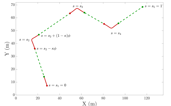
Figure 7: An example showing activation regions of $\tilde{\delta}(s)$. The path is similar to that illustrated in Figure 4. The red segments are segments where $\tilde{\delta}(s)$ is activated. The red dots indicate the points where $s=s_{i}-\tfrac{1}{2}\phi$ and the green ones are points where $s=s_{i}+\tfrac{1}{2}\phi$. In this example we choose $\tilde{d}=15$m.

$$h_{e}=E_{nom}-E-\tfrac{\mathcal{P}(v_{r})}{v_{r}}(L(1-s)-\delta_{m})-\int_{s}^{1}\tilde{\delta}(\tau)d\tau$$ (56)

and applying Leibniz rule to the last term the constraint associated with this candidate CBF is

$$-\mathcal{P}(u)-\Delta_{\omega}+\tfrac{\bar{\mathcal{P}}(v_{r})}{v_{r}}(L\eta-\dot{L}(1-s))+\tilde{\delta}(s)\eta\geq-\gamma_{e}h_{e}$$ (57)

We note that the integrand in (56) can be carried out numerically. Before showing that (56) is a CBF, we need to choose appropriate values for $P_{i}$ in (54) and $\tilde{d}$, both calling for an estimate for a bound on rotation speed of a robot near a waypoint.

Lemma 5.

For a unicycle type robot with kinematics described in (48), applying the transformation (49) and (50) to follow a single integrator control input of a point moving with a speed $v_{r}$ along the path, the rotation speed at a waypoint $w_{i}$ is

$$\omega_{i}\leq\frac{v_{r}}{\ell}\sin\psi_{i}$$ (58)

where $\psi$ is defined in (45).

Proof.

We start by considering $0\leq\psi\leq\tfrac{\pi}{2}$. Without loss of generality, suppose there is a robot at origin with $\theta=0$ (aligned with x-axis), and $u=v_{r}\begin{bmatrix}\cos\psi&\sin\psi\end{bmatrix}^{T}$. From (49) we have

$$\omega=\frac{v_{r}}{\ell}\left(\cos\theta\sin\psi-\sin\theta\cos\psi\right)=\frac{v_{r}}{\ell}\sin(\psi-\theta)$$ (59)

Consider the Lyapunov function $V=\alpha^{2}$ where $\alpha=\psi-\theta$, then $\dot{V}=-2\alpha\dot{\theta}=-2\tfrac{v_{r}}{\ell}\alpha\sin\alpha\leq 0$ and since $\dot{V}=0$ only at $\alpha=0$ then $\alpha$ converges to $\alpha=0$ by virtue of Lasalle’s invariance principle, meaning that $\alpha$, and hence $\omega$, monotonically decrease for $\psi\leq\tfrac{\pi}{2}$. We are interested in finding the maximum value of $\omega$, so by differentiating (59)

$$\frac{d\omega}{d\theta}=-\frac{v_{r}}{\ell}\cos(\psi-\theta)=0\Rightarrow\theta^{*}=\psi-\frac{\pi}{2}.$$ (60)

Since we are considering $\psi\leq\tfrac{\pi}{2}$, it follows that $\theta^{*}\leq 0$. However, since we consider that the robot starts at $\theta=0$ and that $\omega$ monotonically decreases, then we can take $\theta^{*}=0$, meaning $\omega$ is maximum at $\theta=0$. Thus

$$\omega\leq\omega^{*}=\tfrac{v_{r}}{\ell}\sin\psi$$ (61)

If the robot is at waypoint $w_{i}$ pointed to the direction of vector $\Delta w_{i-1}^{i}=w_{i}-w_{i-1}$, there is always a rotation of axes from the global axes to new ones where $\theta=0$ and translation of axes to place $w_{i}$ at the origin, and we reach the same result in (61). The lemma follows by choosing $\psi=\psi_{i}$. We note that the same result holds for $-\tfrac{\pi}{2}\leq\psi<0$, but $\omega$ changes sign by virtue of (50). For $\tfrac{\pi}{2}<\psi<\pi$, from (49) $v<0$ and therefore $\omega^{\prime}=-\tfrac{v_{r}}{\ell}\sin(\psi-\theta)=\tfrac{v_{r}}{\ell}\sin((\psi-\pi)-\theta)$. Using the same procedure but for angle $(\psi-\pi)<0$ we get the same result. ∎

We can use the upper bound estimate of rotation speed near a waypoint $w_{i}$ to estimate an upper bound for the power consumed during a rotation $\Delta_{\omega}$

$$\Delta_{\omega}=\mathcal{P}_{u}(0,\tfrac{v_{r}}{\ell}\sin\psi)$$ (62)

In the following we estimate the activation distance $\tilde{d}$ near a waypoint $w_{i}$.

Proposition 4.

For a robot with model (48) and applying (49) and (50) to follow a single integrator control input for a point moving with speed $v_{r}$ along the path, the distance needed till attenuation of angular speed, i.e. $\omega\leq\tfrac{v_{r}}{\ell}\epsilon_{\omega}$ with $\epsilon_{\omega}$ being an arbitrarily small number, is

$$d_{a}\leq\ell\frac{\pi}{2}\log\frac{\psi_{i}}{\epsilon_{\omega}}$$ (63)

Proof.

We use the candidate Lyapunov function $V=\alpha^{2}=(\psi_{i}-\theta)^{2}$, so $\dot{V}=2\tfrac{v_{r}}{\ell}\alpha\sin\alpha$. One result of (50) is that $\alpha\in[-\tfrac{\pi}{2},\tfrac{\pi}{2}]$ as discussed in proof of Lemma 5. We can prove exponential stability for the candidate Lyapunov function if we can find $k_{1},k_{2},k_{3}>0$ such that (Khalil, 2002)

$$\begin{split}&k_{1}\alpha^{2}\leq V\leq k_{2}\alpha_{2}\\ &\dot{V}\leq-k_{3}\alpha^{2}\end{split}$$ (64)

Since $V=\alpha^{2}$, then $k_{1}=k_{2}=1$. We can estimate $k_{3}$ by letting the parabola $f(\alpha)=k_{3}\alpha^{2}$ and $g(\alpha)=\tfrac{2v_{r}}{\ell}\alpha\sin\alpha$ intersect at $\alpha=\tfrac{\pi}{2}$, which gives $k_{3}=\tfrac{4v_{r}}{\ell\pi}$. By virtue of $V$ being exponentially stable on $\alpha\in[-\tfrac{\pi}{2},\tfrac{\pi}{2}]$, then

$$\alpha\leq\psi_{i}e^{-\tfrac{k_{3}}{2}t}$$ (65)

then at time $\tilde{t}$ the right hand side of the last inequality is equal to $\epsilon_{\omega}$

$$\psi_{i}e^{-\tfrac{k_{3}}{2}\tilde{t}}=\epsilon_{\omega}\Rightarrow\tilde{t}=\tfrac{2}{k_{3}}\log\tfrac{\psi_{i}}{\epsilon_{\omega}}$$ (66)

and we note that $\alpha<\epsilon_{\omega}$ at $t>\tilde{t}$. The attenuation distance then is

$$d_{a}\leq\tilde{d}_{a}=\tilde{t}v_{r}=\ell\frac{\pi}{2}\log\frac{\psi_{i}}{\epsilon_{\omega}}$$ (67)

We note that at $t=\tilde{t}$ the angular speed will be

$$\omega\leq\frac{v_{r}}{\ell}\sin\epsilon_{\omega}\approx\frac{v_{r}}{\ell}\epsilon_{\omega}$$ (68)

∎

Theorem 4.

For a robot with unicycle kinematics, applying (49) and (50), and provided that $\tilde{\delta}$ in (54) is formed such that

$$\tilde{\delta}\geq\frac{L}{v_{r}}\left(\sum_{i=1}^{n_{w}-1}\mathcal{P}_{u}(0,\tfrac{v_{r}}{\ell}\sin\psi_{i})\tilde{\sigma}(s)+\Delta_{\epsilon}\right)$$ (69)

and $\tilde{d}=2\max\{\tilde{d}_{a},d\}$, where $d$ is the tracking distance from (19) and $\Delta_{\epsilon}$ is robot’s power consumption when $\omega=\epsilon_{\omega}$, and if $v_{r}^{*}=\sqrt{\frac{m_{0}}{m_{2}}}\leq u_{\text{max}}$, with $u_{max}>0$ being maximum robot speed, then $h_{e}$ in (56) is a ZCBF. Moreover, if (57) is applied in (41) instead of (16), energy sufficiency is guaranteed.

Proof.

We start by considering when the robot moves on a straight line and away from waypoints, i.e. $s_{i-1}+\tfrac{\phi}{2}<s<s_{i}-\tfrac{\phi}{2}$, in which case the proof is similar to proof of lemma 2 since $\mathcal{P}(u)=\mathcal{P}_{u}(v,0)$ as pointed out in remark 2.

We note that when $h_{d}\approx 0$, the robot is following the reference point $x_{r}$ along a straight line and it starts rotating after $x_{r}$ passes waypoint $w_{i}$, i.e. $s\geq s_{i}$, and since $||x-x_{r}||\approx d$ it means that the robot will start rotation a distance $d$ away from $w_{i}$, but since $\tilde{d}=2\max\{\tilde{d}_{a},d\}$, $\tilde{\delta}$ will be activated at a distance greater than or equal $d$ before $w_{i}$ along the path, i.e. before the robot starts spinning. Also when $s_{i}<s\leq s_{i}+\tfrac{\phi}{2}$ and due to choice of $\tilde{d}$, $s=s_{i}+\tfrac{\phi}{2}$ happens at least a distance $\tilde{d}_{a}$ after $w_{i}$ along the path and at this point $\omega<\tfrac{v_{r}}{\ell}\epsilon_{\omega}$, i.e. $\tilde{\delta}$ will be deactivated after $\omega$ has been attenuated.

When $\tilde{\delta}$ is activated, i.e. $s_{i}-\tfrac{\phi}{2}<s<s_{i}+\tfrac{\phi}{2}$, and considering the critical case where $h_{e}\approx 0$ and $h_{d}\approx 0$, similar to what we did in the proof of Lemma 2, we consider the equality of (20) and (57), so from (57) (and noting that $\dot{L}=0$ when the robot is moving along the path by virtue of proposition 2)

$$\eta=\frac{\mathcal{P}(u)+\Delta_{\omega}}{\mathcal{P}(v_{r})+\tilde{\delta}\frac{v_{r}}{L}}\frac{v_{r}}{L}$$ (70)

and doing the same steps to obtain (24)

$$||u||=\frac{\mathcal{P}(u)+\Delta_{\omega}}{\mathcal{P}(v_{r})+\tilde{\delta}\frac{v_{r}}{L}}v_{r}$$ (71)

which is a similar root finding problem to (24). Since $\tilde{\delta}\geq\mathcal{P}_{u}(0,\tfrac{v_{r}}{\ell}\sin\psi_{i})\frac{L}{v_{r}}$, then $\tilde{\delta}\tfrac{v_{r}}{L}\geq\Delta_{\omega}$, which ensures roots for (71) exist and that $||u||$ will converge to a slower speed than $v_{r}$ as discussed in Remark 1 (since having $\tilde{\delta}\tfrac{v_{r}}{L}-\Delta_{\omega}<0$ has a similar effect as having $\Delta_{p}<0$ in Remark 1). Moreover, when $\omega<\tfrac{v_{r}}{\ell}\epsilon_{\omega}$ , (71) will become

$$||u||=\frac{\mathcal{P}(u)+\Delta_{\epsilon}}{\mathcal{P}(v_{r})+\tilde{\delta}\frac{v_{r}}{L}}v_{r}$$ (72)

which is guaranteed to have roots since $\tilde{\delta}\tfrac{v_{r}}{L}\geq\Delta_{\epsilon}$. Thus provided that $\sqrt{\frac{m_{0}}{m_{2}}}\leq u_{\text{max}}$ there is always a value of $u$ that satisfies (57). Since (19) and (56) are ZCBFs and if $\delta$ in (56) is equal to $\delta_{m}$ from (30) then the robot’s energy satisfies $E(t)=E_{nom}$ only when $||x-x_{c}||<\delta$ as discussed in the proof of Theorem 2, thus ensuring energy sufficiency. ∎

We can apply the same quadratic program in (41), but with replacing the definition of energy sufficiency CBF, and for that the $A$ and $B$ matrices in (41) will be

$$\begin{split}\mathbf{A}&=\begin{bmatrix}\tfrac{\mathcal{P}(v_{r})}{v_{r}}L+\tilde{\delta}&\mathbf{0}_{1\times 2}\\ 1&\mathbf{0}_{1\times 2}\\ (x-x_{r})^{T}\tfrac{\partial x_{r}}{\partial s}&-(x-x_{r})^{T}\end{bmatrix}\\ \mathbf{B}&=\begin{bmatrix}-\gamma_{e}h_{e}+\mathcal{P}(u)+\Delta_{\omega}+\dot{L}(1-s)\\ -\gamma_{b}h_{b}\\ -\gamma_{d}h_{d}\end{bmatrix}\\ \mathbf{u}_{nom}&=\begin{bmatrix}0&u_{nom}\end{bmatrix}\end{split}$$ (73)

We can follow the same steps as in Theorem 2 to show that energy sufficiency is maintained solving this QP problem over a fixed path, with the same path freezing idea as in Proposition 2.

The treatment thus far concerns a unicycle robot moving around, with a fixed path back to charging station. A path planner could be used to update the path in the same manner discussed in Section 5. We can use a similar sequence as in Algorithm 1, but we need to show that the SPC method is a valid backup for the proposed unicycle adaptation.

Proposition 5.

Sequential Path Construction does not violate energy sufficiency for a robot described by (48) when applying (41) with transformation (49), (50), and with $A$ and $B$ matrices described in (73).

Proof.

Similar to proposition 3, provided that there exists a value of $u=u_{nom}$ and $\eta=\eta_{nom}$ satisfying following inequalities

$$h_{e}=E_{nom}-E-\tfrac{\mathcal{P}(v_{r})}{v_{r}}(L(1-s)-\delta)-\int_{s}^{1}\tilde{\delta}(\tau)d\tau$$ (74a)

$$-\mathcal{P}(u)-\Delta_{\omega}+\tfrac{\bar{\mathcal{P}}(v_{r})}{v_{r}}(L\eta_{nom}-\dot{L}(1-s))+\tilde{\delta}(s)\eta_{nom}\geq-\gamma_{e}h_{e}$$ (74b)

we need to show that (74b) is not violated at a path update. Similar to proof of Proposition 3, provided that nominal control inputs are continuous and satisfying (74b), then there are no jumps (i.e. instantaneous changes) for $E,\mathcal{P}(u),\Delta_{\omega}$ and $v_{r}$. Moreover since SPC is path length invariant, $L$ does not change. Also since SPC is path angle invariant from Lemma 4, then the increase in power due to the addition of the new waypoint is equal to zero (because $\psi_{2}$ for the new path is equal to zero) and no change occurs for the power consumption along the path, therefore $\tilde{\delta}$ does not jump as well, meaning (74b) is not violated under SPC. ∎

We can apply Algorithm 1 and the same logic in Theorem 3 to show that energy sufficiency is maintained under discrete path updates.

Remark 3.

The adaptation we are using for the method based on single integrator dynamics (in Section 5) to unicycle dynamics is versatile and can go beyond accounting for excess power consumption near waypoints. This is due to the fact that the estimated excess power, e.g. (54), is modelled as a summation of double sigmoid functions, activated along different segments of the path. Moreover, this excess in the estimated power consumption is incorporated in the energy sufficiency CBF (56) through numerical integration, making it easier to account for different types of “resistance” along the path. For example, effects like surface inclinations, variability in friction and increased processing power, among many others, could be modelled in a similar way to (54) through identifying ranges of the path parameter $s$ corresponding to different segments on the path, each associated with a double sigmoid function multiplied by the estimated power consumption related to the effect being modelled. This idea allows to adapt the methods based on single integrator dynamics to a wide range of scenarios, environments and robot types.

7 Results

7.1 Simulation Setup

We present the simulation results that highlight the ability of our proposed framework to ensure energy sufficiency during an exploration mission. The considered experimental scenario allows the robots to perform the exploration mission while ensuring robot’s energy consumption is within the dedicated energy budget $E_{nom}$.

We evaluate the approach using a physics-based simulator (Pinciroli et al., 2012). We use a simulated KheperaIV robot equipped with a 2D lidar with a field of view of 210 degrees and a 4m range as the primary perception sensor. The architecture of the autonomy software used in simulations is shown in Figure 8A. The autonomy software allows the robot to explore and map the environment. Each robot is equipped with a volumetric mapping system (Oleynikova et al., 2017, Voxblox) using Truncated Signed Distance Fields to map the environment. A graph-based exploration planner (GBPlanner, Dang et al., 2019) uses the mapping system to plan both the exploration and homing trajectories. We carry out a path shortening procedure as described in (Cimurs et al., 2017, Algorithm 1) to eliminate redundant and unnecessary points from the original path planner output, making the final path straighter and shorter. Our proposed framework is implemented as a Buzz (Pinciroli and Beltrame, 2016) script that periodically queries the exploration planner for a path and applies the required control commands to the robot.

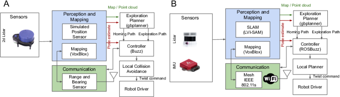
Figure 8: Software Architecture used during the simulation study (A) and on the experimental hardware (B).

We use the maze map benchmarks from (Sturtevant, 2012) as a blueprint for obstacles in the environment, and each map is scaled so that it fits a square area of $30\times 30$ meters. In each simulation one robot maps the unexplored portions of the map to maximize its volumetric gain (Dang et al., 2019). We run four groups of experiments for three different maps from the benchmarking dataset (Sturtevant, 2012), and for each case we run 50 simulations with randomized configurations to obtain a statistically valid dataset.

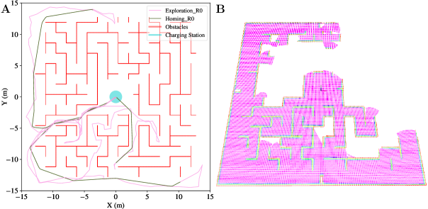
Figure 9: A sample result for the trajectories generated by the robot (A) and the map constructed in the same simulation run (B) for an exploration task in a maze environment (maze-4 from (Sturtevant, 2012)), while using our proposed approach to maintain energy sufficiency.

We use a polynomial power model to describe power consumption of the robots in simulation. We derive this model by collecting power consumption readings from a physical AgileX Scout Mini (AgileX, 2023) robot at different values of linear and angular speed, then we fit a surface through these readings to obtain out power model. Figure 10 shows the fitted power model, along with the actual collected power readings from the robot. We interface the single integrator output $\mathbf{u}^{*}$ of (41) to the unicycle model of the robots using the transformation (49) and the modification (50). We use the robot’s linear and angular speeds to estimate the robot’s power according to the following polynomial

$$\begin{split}\mathcal{P}_{u}(v,\omega)&=27.8126||v||^{2}-107.7343|\omega|^{2}\\ &+31.4578||v||+179.9095|\omega|+1.234\end{split}$$ (75)

and the power model is depicted in Figure 10. We also add to this model an additional power of $\mathcal{P}_{payload}=20$W to account for payload power consumption.

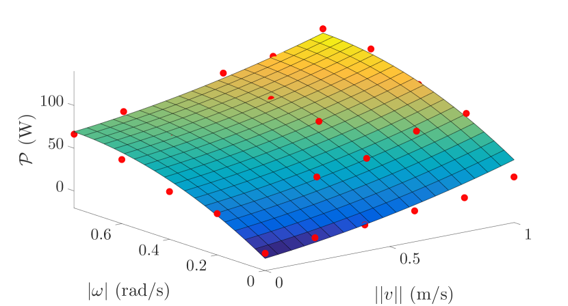
Figure 10: Surface plot of the power model used in simulation. The red dots are the actual measured power values at different values of linear and angular speeds ($v$ and $\omega$) and is fitted by a 3 dimensional surface to minimize the mean least square error between the model and the real data points.

7.2 Simulation Results

Figure 9 shows an example of the robots’ trajectory during exploration and returning to the charging station for one simulation run in one of the maze environments (maze-4). Figure 9 also shows the map built by the robot during this simulation run. As observed in the trajectory plot, any given robot’s exploration trajectory is always accompanied by a homing trajectory to the charging station satisfying the energy constraints.

For all simulation runs we measure the estimated Total Area Covered (TAC) and the Energy On Arrival (EOA), which is the amount of energy consumed by the robot by the time it arrives back to the station, and we use these values as metrics for performance. The TAC serves as a measure of the mission execution quality, and the EOA is a measure of the extent the available energy budget has been used. We run all test cases at two desired values of return speed: a slow speed of $v_{r}=0.1$m/s and a faster speed of $v_{r}=0.5$m/s. We highlight the efficacy of our approach by comparing the aforementioned metrics to the results of a baseline method in which a robot returns back on the path when the available energy reaches a certain fixed threshold percentage of the total nominal energy (as it is a standard procedure with commercial robots). For the baseline we use only the tracking CBF (19) in a QP problem similar to (41) and we change the path parameter $s$ according to the following relation

$$\dot{s}=\begin{cases}\frac{v_{r}}{L},\quad\text{if}\quad\tfrac{E}{E_{nom}}>\tau\\ 0,\quad\text{otherwise}\end{cases}$$ (76)

where $0<\tau<1$ is a threshold return energy ratio, and $L$ is the total path length at the point when the robot starts moving back towards the charging station. We show the results of our comparison for the aggregated values of TAC for different simulation scenarios in Figure 11(a). To highlight the relation between TAC and EOA we use red dots in Figure 11(a) to indicate TAC values corresponding to simulation runs during which the energy budget is violated, i.e. EOA is less than zero at least once, indicating the robot’s failure to recharge before its energy budget is fully consumed. Figure 11(b) and  11(c) show histograms of EOA values distribution for our method as well as baseline at different values of $\tau$ for $v_{r}=0.5$m/s and $v_{r}=0.1$m/s respectively. In all simulation runs the total energy budget is set to be $12$kJ.

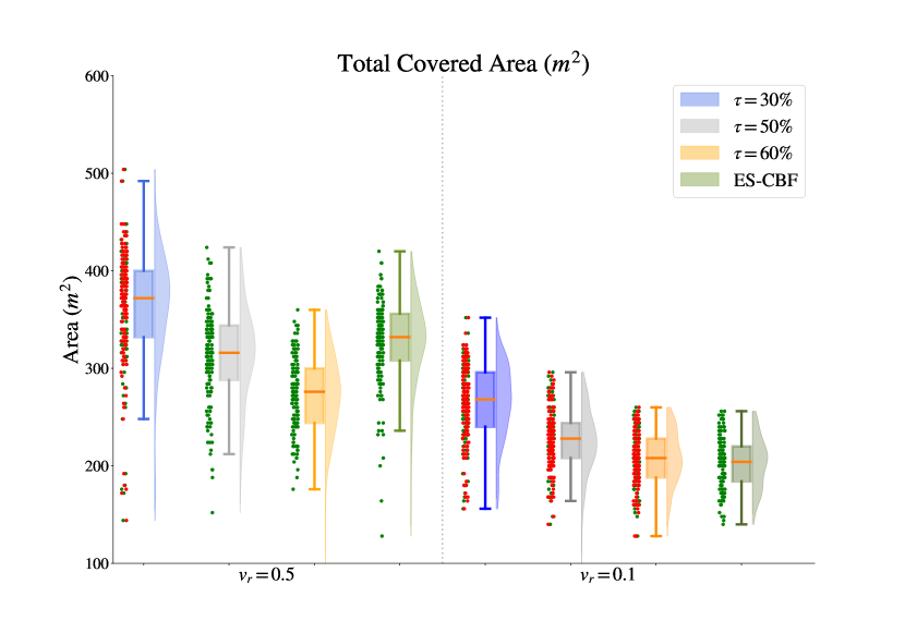
(a) Estimated total area covered

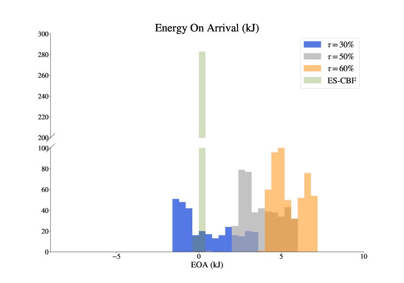
(b) Energy on arrival for simulations with $v_{r}=0.5$m/s.

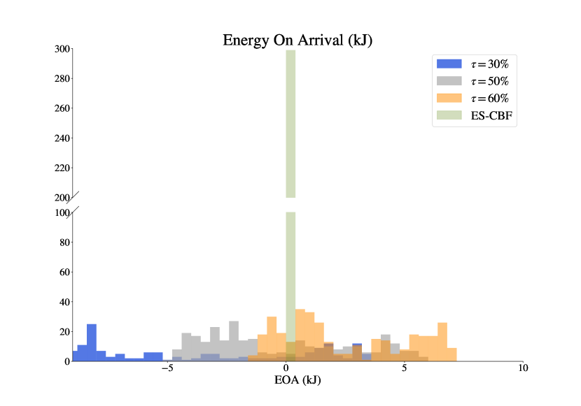
(c) Energy on arrival for simulations with $v_{r}=0.1$m/s.

Figure 11: Comparison between baseline method for three different threshold percentages $\tau$ and our CBF-based approach for energy sufficiency, denoted ES-CBF. Simulation data for total area covered and energy values upon arrival to charging station is collected for three test environments and two different desired return speeds ($v_{r}=0.5$m/s and $v_{r}=0.1$m/s), each run for 50 instances with different random seeds. The red dots in Figure 11(a) indicate area values corresponding to simulation instances where the energy budget is violated at least once, while green dots indicate no violation of energy budget. Histograms  11(b) and  11(c) show distribution of energy on arrival (EOA) values for $v_{r}=0.5$m/s and $v_{r}=0.1$m/s respectively.

We note that in Figure 11(a) for $v_{r}=0.1$m/s the area covered consistently increases with decreasing return energy threshold percentages, i.e. when a robot starts returning to recharge at $\tau=0.3$ it typically covers more area than when it needs to return at $\tau=0.5$ as it uses more of its energy to carry out its mission. Although for this case the area covered using our proposed method is less than baseline (box plot median value of 268m² for $\tau=0.3$ and 204m² for ES-CBF, meaning a 24% reduction in TAC in the worst case), baseline results have significantly more red dots than ES-CBF, indicating significantly more violations of energy budget than ES-CBF, so although TAC is more for baseline the energy budget is violated for most test runs.

For $v_{r}=0.5$m/s, Figure 11(a) shows an overall increase in TAC for both baseline and ES-CBF compared to the case where $v_{r}=0.1$m/s. Moreover, we notice an increase in TAC in case of ES-CBF over baseline with $\tau=0.5$ and $\tau=0.6$ (5% and 20% increase in TAC respectively), while there is a decrease of 10% in TAC between baseline with $\tau=0.3$ and ES-CBF. For baseline cases with $\tau=0.5$ and $\tau=0.6$ there are no red dots at $v_{r}$=0.5m/s in Figure 11(a), but there are numerous violations of energy sufficiency for baseline with $\tau=0.3$. Overall, choosing a threshold value to return to the charging station depends on the map and task at hand, and does not provide guarantees for either optimal mission success or return or respecting the energy budget. On the contrary, our method guarantees that the energy budget is fully exploited, without affecting mission performance.

It is also worth noting from Figure 11(b) and 11(c) that the distribution of EOA values is very tight around zero, meaning that robots applying ES-CBF framework arrive to the station without violating the energy budget allocated and without wasting energy, i.e. robots do not arrive too late or too early, which means full utilization of the energy allocated. On the other hand for the baseline method we can see in Figure 11(c) for $v_{r}=0.1$ that EOA values are more widely dispersed around zero, with a significant portion of the values being positive or negative, indicating robots arriving to station either too early or too late, which is a direct result of not considering needed energy to return back to station (e.g. a robot could reach the return threshold $\tau$ when it is relatively close to the station so it will eventually arrive back with a significant amount of energy, and it may reach $\tau$ when it is far away so that the energy budget is fully depleted on the way back). We also note that for $v_{r}=0.5$m/s the values of EOA are mostly positive for baseline with $\tau=0.5$ and $\tau=0.6$ indicating significant non-utilized energy when the robot returns back to recharge. Therefore for these two baseline cases the robots utilize less energy for exploration and this explains the advantage that ES-CBF has in TAC over these two baseline cases at $v_{r}=0.5$m/s.

7.3 Hardware setup

We study the performance of the energy-sufficiency approach using an AgileX Scout Mini rover equipped with a mission payload to perform exploration and mapping missions, shown in Figure 12. The robot has an Ouster OS0-64 lidar as the primary perception sensor and a high-performance Inertial Measurement Unit (IMU) from VectorNav. A mesh communication router implements IEEE802.11s to communicate with the base station.

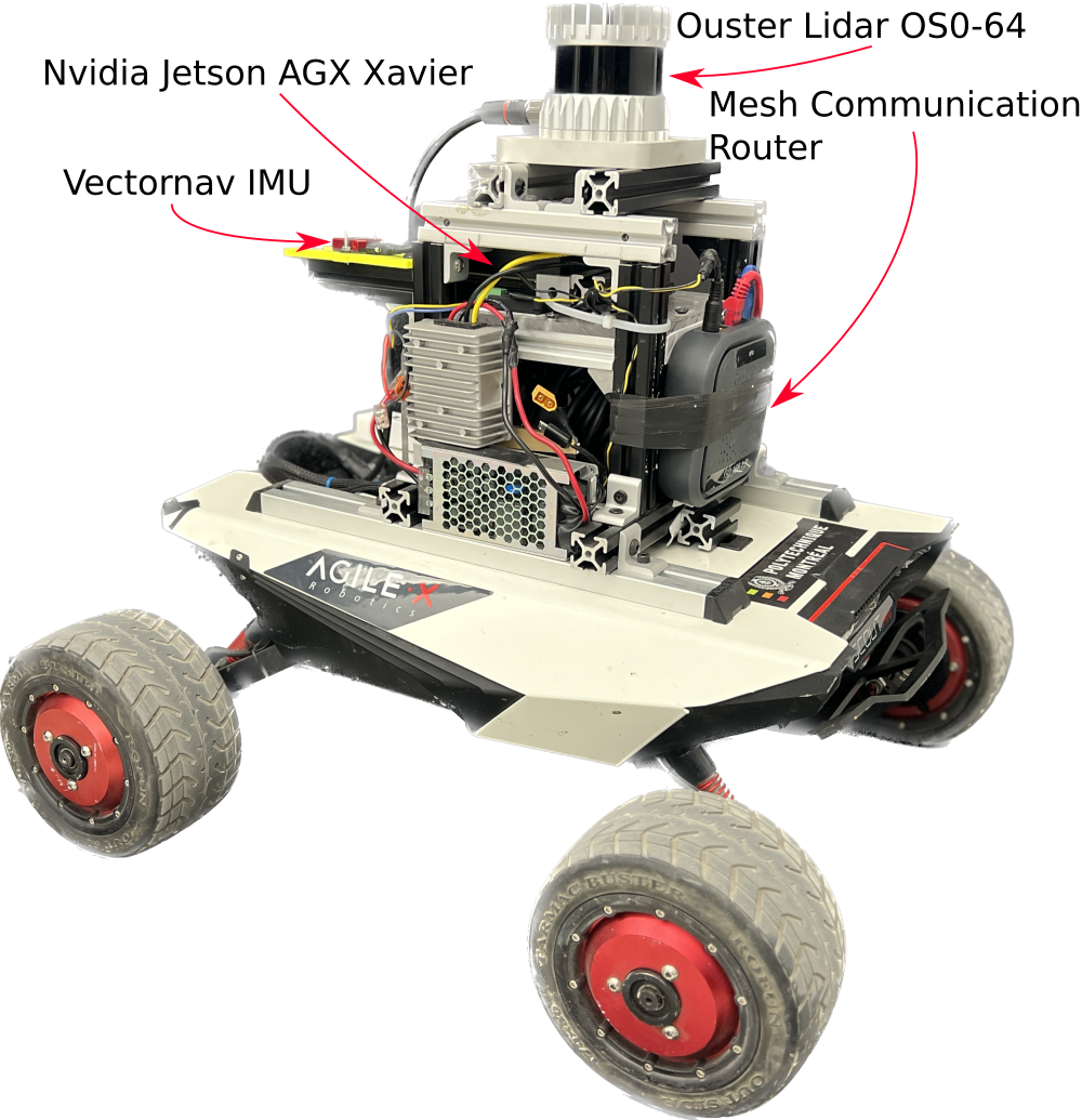
Figure 12: Experimental setup we use to perform the exploration mission while maintaining energy sufficiency. It consists of an AgileX Scout Mini rover with a mission payload mounted on top as demonstrated above.

Figure 8B shows the software architecture deployed on the Nvidia Jetson AGX Xavier of the rover. We implement a full stack Simultaneous Localization And Mapping (SLAM) system, mesh communication system, and a local planner for collision avoidance. Unlike the simulation, the rover performs a full-stack 3D localization and mapping using a variant of LVI_SAM (Shan et al., 2021) with a front-end generating pose graphs and a back-end performing map optimization. The mapping (Oleynikova et al., 2017, Voxblox) and planning (Gbplanner modules and controller were the same for both simulation and hardware. We apply the path shortening procedure in (Cimurs et al., 2017, Algorithm 1) on the output of the path planner, as we do in the simulation setup.

We estimate the robot’s power consumption using voltage and electric current values. Upon arrival to charging region the robot executes a simple docking manoeuvre to enter the charging region and carries out a simulated battery swap operation to replenish the robot’s energy. We point out that such setup does not affect the validity of the experiment and could be justified by the fact that the energy consumed by the robot is consistent, meaning that the power needed to move the robot at a certain speed does not depend on the battery, but rather depends on the robot’s mechanical properties and the environment which are both static.

7.4 Hardware results

We apply the proposed method on our experimental setup and we show the results in Figure 13, as well as the point cloud map for the experimental run in Figure 1. In this experiment the robot is tasked with exploring and mapping a set of corridors and hallways while returning back to a charging spot. The map generated by the robot and the trajectories taken by the robot during an experimental run are shown in Figure 1.

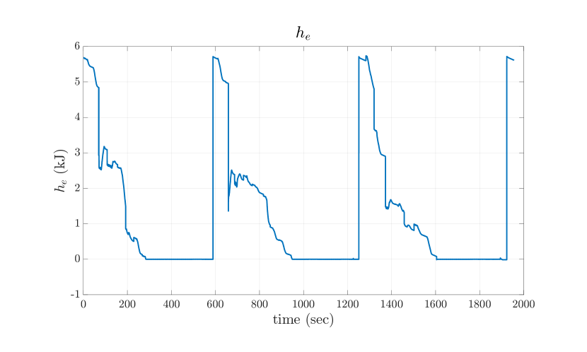
(a) Energy sufficiency CBF ($h_{e}$)

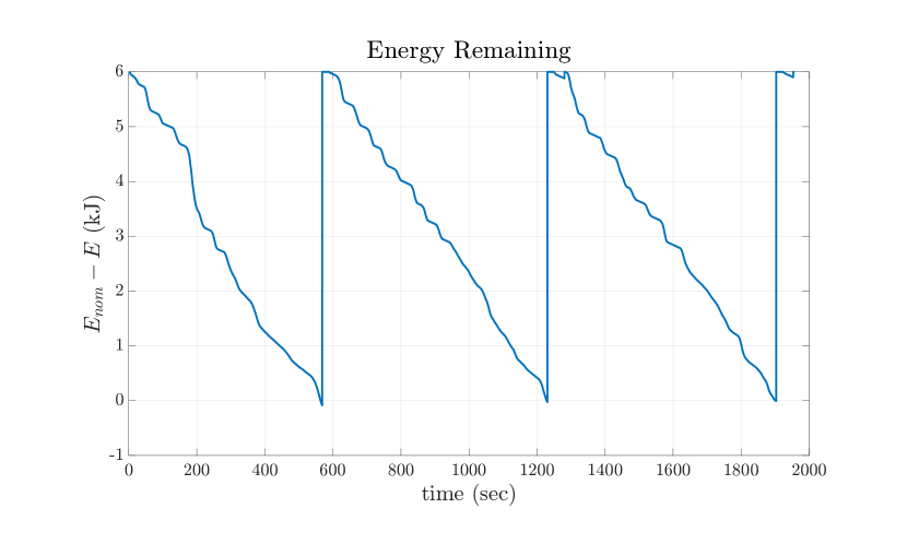
(b) Remaining energy

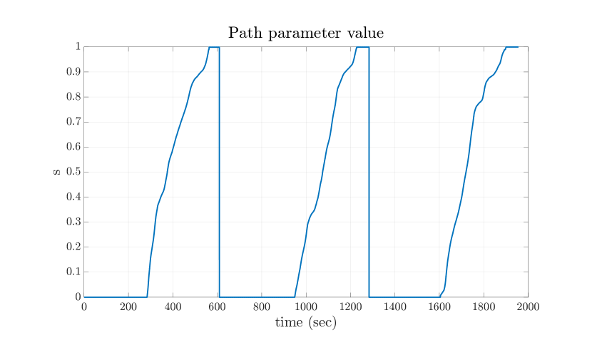
(c) Path parameter

(d) Path length

Figure 13: Results from robot experiment. We emphasize the fact that the robot returns back to station with a depleted battery, meaning that our proposed framework is capable of maintaining energy sufficiency.

For this experiment the allocated energy budget is 7kJ and the desired return speed was set to $v_{r}=0.2$m/s. We note from Figure 13(b) that the robot consumes the energy budget fully by the time it arrives back to recharge, which shows the ability of our proposed approach to maintain energy sufficiency in cluttered environments. From Figure 13(c) the path parameter value is equal to zero as long as the energy sufficiency constraint (16) is not violated, then when $h_{e}\approx 0$ (in Figure 13(a), indicating energy sufficiency being close to the boundary of its safe set) it starts to increase and drive the robot back towards the station along the path. Figure 1 shows examples of paths taken by the robot while exploring its environment.

8 Conclusions

In this work we present a CBF based method that provides guarantees on energy sufficiency of a ground robot in an unknown and unstructured environment. Our approach is to augment a sampling based path planner (like GBplanner, Dang et al., 2019) by a CBF layer, extending our work (Fouad and Beltrame, 2022) to endow a robot with the ability to move along a path in an energy aware manner such that the total energy consumed does not exceed a predefined threshold. We described a continuous representation for piecewise continuous paths produced by a path planner. We define a reference point that slides along this continuous path depending on robot’s energy. We show the relationship between the constraints for controlling both the reference point and robot’s position and show conditions for these constraints to complement each other. We demonstrate how these ideas are valid for dynamic cases in which the path planner updates the path frequently and the robot is carrying out a mission. Finally we demonstrate a method for adapting our framework, based on a single integrator model, to a unicycle model. We highlight through simulation and experimental results the ability of our method to deal with unknown and unstructured environments while maintaining energy sufficiency.

Our proposed framework has the advantage of flexibility and adaptability to different types of robot models and environments. Such framework can be useful in many application where long term autonomy is needed, e.g. underground and cave exploration, robot reinforcement learning, self driving cars in urban environments, and many others.

As a future work we plan to extend our framework to be able to handle coordination between multiple robots to share a charging station in the same spirit as Fouad and Beltrame 2022, while being able to deal with unstructured and complex environments. Another direction could be using online estimation and learning techniques to handle power models that are variable by nature and need constant adaptation, such as wind fields, snowy conditions, etc.

9 Acknowledgements

The authors would like to thank Koresh Khateri for his useful insights and fruitful discussions, as well as Sameh Darwish and Karthik Soma for their help with the experiments.

10 Declaration of conflicting interests

The Authors declare that there is no conflict of interest.

11 Funding

This work was supported by the National Science and Engineering Research Council of Canada [Discovery Grant number 2019-05165].

References

- AgileX (2023) AgileX (2023) Scout Mini. https://global.agilex.ai/products/scout-mini [Accessed: Jun 2023].
- Alizadeh et al. (2014) Alizadeh M, Wai HT, Scaglione A, Goldsmith A, Fan YY and Javidi T (2014) Optimized path planning for electric vehicle routing and charging. In: 2014 52nd Annual Allerton Conference on Communication, Control, and Computing (Allerton). pp. 25–32. 10.1109/ALLERTON.2014.7028431.
- Ames et al. (2019) Ames AD, Coogan S, Egerstedt M, Notomista G, Sreenath K and Tabuada P (2019) Control barrier functions: Theory and applications. In: 2019 18th European control conference (ECC). IEEE, pp. 3420–3431.
- Ames et al. (2014) Ames AD, Grizzle JW and Tabuada P (2014) Control barrier function based quadratic programs with application to adaptive cruise control. In: 53rd IEEE Conference on Decision and Control. IEEE, pp. 6271–6278.
- Bajracharya et al. (2008) Bajracharya M, Maimone MW and Helmick D (2008) Autonomy for mars rovers: Past, present, and future. Computer 41(12): 44–50.
- Balta et al. (2017) Balta H, Bedkowski J, Govindaraj S, Majek K, Musialik P, Serrano D, Alexis K, Siegwart R and De Cubber G (2017) Integrated data management for a fleet of search-and-rescue robots. Journal of Field Robotics 34(3): 539–582.
- Best et al. (2022) Best G, Garg R, Keller J, Hollinger GA and Scherer S (2022) Resilient multi-sensor exploration of multifarious environments with a team of aerial robots. In: Proceedings of Robotics: Science and Systems.
- Bircher et al. (2016) Bircher A, Kamel M, Alexis K, Oleynikova H and Siegwart R (2016) Receding horizon” next-best-view” planner for 3d exploration. In: 2016 IEEE international conference on robotics and automation (ICRA). IEEE, pp. 1462–1468.
- Cao et al. (2021) Cao C, Zhu H, Choset H and Zhang J (2021) Tare: A hierarchical framework for efficiently exploring complex 3d environments. In: Robotics: Science and Systems, volume 5.
- Cimurs et al. (2017) Cimurs R, Hwang J and Suh IH (2017) Bezier curve-based smoothing for path planner with curvature constraint. In: 2017 First IEEE International Conference on Robotic Computing (IRC). IEEE, pp. 241–248.
- Cushing et al. (2012) Cushing GE et al. (2012) Candidate cave entrances on mars. Journal of Cave and Karst Studies 74(1): 33–47.
- Dang et al. (2019) Dang T, Mascarich F, Khattak S, Papachristos C and Alexis K (2019) Graph-based path planning for autonomous robotic exploration in subterranean environments. In: 2019 IEEE/RSJ International Conference on Intelligent Robots and Systems (IROS). IEEE, pp. 3105–3112.
- DARPA (2018) DARPA (2018) DARPA Subterranean Challenge. https://www.subtchallenge.com. Online; accessed 8 March 2023.
- Dharmadhikari et al. (2020) Dharmadhikari M, Dang T, Solanka L, Loje J, Nguyen H, Khedekar N and Alexis K (2020) Motion primitives-based path planning for fast and agile exploration using aerial robots. In: 2020 IEEE International Conference on Robotics and Automation (ICRA). IEEE, pp. 179–185.
- Ding et al. (2019) Ding Y, Luo W and Sycara K (2019) Decentralized multiple mobile depots route planning for replenishing persistent surveillance robots. In: 2019 International Symposium on Multi-Robot and Multi-Agent Systems (MRS). IEEE, pp. 23–29.
- Elhoseny et al. (2018) Elhoseny M, Tharwat A and Hassanien AE (2018) Bezier curve based path planning in a dynamic field using modified genetic algorithm. Journal of Computational Science 25: 339–350.
- Forsgren et al. (2002) Forsgren A, Gill PE and Wright MH (2002) Interior methods for nonlinear optimization. SIAM review 44(4): 525–597.
- Fouad and Beltrame (2020) Fouad H and Beltrame G (2020) Energy autonomy for resource-constrained multi robot missions. In: 2020 IEEE/RSJ International Conference on Intelligent Robots and Systems (IROS). IEEE, pp. 7006–7013.
- Fouad and Beltrame (2022) Fouad H and Beltrame G (2022) Energy autonomy for robot systems with constrained resources. IEEE Transactions on Robotics .
- Fu and Dong (2019) Fu F and Dong H (2019) Targeted optimal-path problem for electric vehicles with connected charging stations. PLOS ONE 14(8): e0220361. 10.1371/journal.pone.0220361. URL https://dx.plos.org/10.1371/journal.pone.0220361.
- Fu et al. (2015) Fu M, Song W, Yi Y and Wang M (2015) Path planning and decision making for autonomous vehicle in urban environment. In: 2015 IEEE 18th international conference on intelligent transportation systems. IEEE, pp. 686–692.
- Gruning et al. (2020) Gruning V, Pentzer J, Brennan S and Reichard K (2020) Energy-aware path planning for skid-steer robots operating on hilly terrain. In: 2020 American Control Conference (ACC). IEEE, pp. 2094–2099.
- Hao et al. (2021) Hao B, Du H, Dai X and Liang H (2021) Automatic recharging path planning for cleaning robots. Mobile Information Systems 2021.
- Jaroszek and Trojnacki (2014) Jaroszek P and Trojnacki M (2014) Model–based energy efficient global path planning for a four–wheeled mobile robot. Control and Cybernetics 43(2).
- Kamra et al. (2017) Kamra N, Kumar TS and Ayanian N (2017) Combinatorial problems in multirobot battery exchange systems. IEEE Transactions on Automation Science and Engineering 15(2): 852–862.
- Khalil (2002) Khalil HK (2002) Nonlinear systems; 3rd ed. Upper Saddle River, NJ: Prentice-Hall. URL https://cds.cern.ch/record/1173048. The book can be consulted by contacting: PH-AID: Wallet, Lionel.
- Kundu and Saha (2021) Kundu T and Saha I (2021) Mobile recharger path planning and recharge scheduling in a multi-robot environment. In: 2021 IEEE/RSJ International Conference on Intelligent Robots and Systems (IROS). IEEE, pp. 3635–3642.
- Li et al. (2018) Li B, Patankar S, Moridian B and Mahmoudian N (2018) Planning large-scale search and rescue using team of uavs and charging stations. In: 2018 IEEE international symposium on safety, security, and rescue robotics (SSRR). IEEE, pp. 1–8.
- Liu et al. (2014) Liu F, Liang S and Xian DX (2014) Optimal path planning for mobile robot using tailored genetic algorithm. TELKOMNIKA Indonesian Journal of Electrical Engineering 12(1): 1–9.
- Mathew et al. (2015) Mathew N, Smith SL and Waslander SL (2015) Multirobot rendezvous planning for recharging in persistent tasks. IEEE Transactions on Robotics 31(1): 128–142.
- Mehta et al. (2015) Mehta SS, Ton C, McCourt MJ, Kan Z, Doucette EA and Curtis W (2015) Human-assisted rrt for path planning in urban environments. In: 2015 IEEE International Conference on Systems, Man, and Cybernetics. IEEE, pp. 941–946.
- Noreen (2020) Noreen I (2020) Collision free smooth path for mobile robots in cluttered environment using an economical clamped cubic b-spline. Symmetry 12(9): 1567.
- Notomista et al. (2018) Notomista G, Ruf SF and Egerstedt M (2018) Persistification of robotic tasks using control barrier functions. IEEE Robotics and Automation Letters 3(2): 758–763.
- Ogren et al. (2001) Ogren P, Egerstedt M and Hu X (2001) A control lyapunov function approach to multi-agent coordination. In: Proceedings of the 40th IEEE Conference on Decision and Control (Cat. No. 01CH37228), volume 2. IEEE, pp. 1150–1155.
- Oleynikova et al. (2017) Oleynikova H, Taylor Z, Fehr M, Siegwart R and Nieto J (2017) Voxblox: Incremental 3d euclidean signed distance fields for on-board mav planning. In: IEEE/RSJ International Conference on Intelligent Robots and Systems (IROS).
- Patle et al. (2019) Patle B, Pandey A, Parhi D, Jagadeesh A et al. (2019) A review: On path planning strategies for navigation of mobile robot. Defence Technology 15(4): 582–606.
- Pinciroli and Beltrame (2016) Pinciroli C and Beltrame G (2016) Buzz: An extensible programming language for heterogeneous swarm robotics. In: 2016 IEEE/RSJ International Conference on Intelligent Robots and Systems (IROS). IEEE, pp. 3794–3800.
- Pinciroli et al. (2012) Pinciroli C, Trianni V, O’Grady R, Pini G, Brutschy A, Brambilla M, Mathews N, Ferrante E, Di Caro G, Ducatelle F et al. (2012) Argos: a modular, parallel, multi-engine simulator for multi-robot systems. Swarm intelligence 6(4): 271–295.
- Prajna and Jadbabaie (2004) Prajna S and Jadbabaie A (2004) Safety verification of hybrid systems using barrier certificates. In: International Workshop on Hybrid Systems: Computation and Control. Springer, pp. 477–492.
- Ramana et al. (2016) Ramana M, Varma SA and Kothari M (2016) Motion planning for a fixed-wing uav in urban environments. IFAC-PapersOnLine 49(1): 419–424.
- Ravankar et al. (2018) Ravankar A, Ravankar AA, Kobayashi Y, Hoshino Y and Peng CC (2018) Path smoothing techniques in robot navigation: State-of-the-art, current and future challenges. Sensors 18(9): 3170.
- Ravankar et al. (2021) Ravankar A, Ravankar AA, Watanabe M, Hoshino Y and Rawankar A (2021) Multi-robot path planning for smart access of distributed charging points in map. Artificial Life and Robotics 26(1): 52–60.
- Romdlony and Jayawardhana (2014) Romdlony MZ and Jayawardhana B (2014) Uniting control lyapunov and control barrier functions. In: 53rd IEEE Conference on Decision and Control. IEEE, pp. 2293–2298.
- Satai et al. (2021) Satai HA, Zahra MMA, Rasool ZI, Abd-Ali RS and Pruncu CI (2021) Bézier curves-based optimal trajectory design for multirotor uavs with any-angle pathfinding algorithms. Sensors 21(7): 2460.
- Schneider et al. (2014) Schneider M, Stenger A and Goeke D (2014) The electric vehicle-routing problem with time windows and recharging stations. Transportation science 48(4): 500–520.
- Shan et al. (2021) Shan T, Englot B, Ratti C and Daniela R (2021) Lvi-sam: Tightly-coupled lidar-visual-inertial odometry via smoothing and mapping. In: IEEE International Conference on Robotics and Automation (ICRA). IEEE, pp. 5692–5698.
- Simba et al. (2016) Simba KR, Uchiyama N and Sano S (2016) Real-time smooth trajectory generation for nonholonomic mobile robots using bézier curves. Robotics and Computer-Integrated Manufacturing 41: 31–42.
- Souissi et al. (2013) Souissi O, Benatitallah R, Duvivier D, Artiba A, Belanger N and Feyzeau P (2013) Path planning: A 2013 survey. In: Proceedings of 2013 International Conference on Industrial Engineering and Systems Management (IESM). IEEE, pp. 1–8.
- Sturtevant (2012) Sturtevant N (2012) Benchmarks for grid-based pathfinding. Transactions on Computational Intelligence and AI in Games 4(2): 144 – 148. URL http://web.cs.du.edu/~sturtevant/papers/benchmarks.pdf.
- Thrun et al. (2004) Thrun S, Thayer S, Whittaker W, Baker C, Burgard W, Ferguson D, Hahnel D, Montemerlo D, Morris A, Omohundro Z et al. (2004) Autonomous exploration and mapping of abandoned mines. IEEE Robotics & Automation Magazine 11(4): 79–91.
- Titus et al. (2021) Titus T, Wynne JJ, Boston P, De Leon P, Demirel-Floyd C, Jones H, Sauro F, Uckert K, Aghamohammadi A, Alexander C et al. (2021) Science and technology requirements to explore caves in our solar system. Bulletin of the American Astronomical Society 53(4).
- Wang et al. (2008) Wang T, Wang B, Wei H, Cao Y, Wang M and Shao Z (2008) Staying-alive and energy-efficient path planning for mobile robots. In: 2008 American Control Conference. pp. 868–873. 10.1109/ACC.2008.4586602. ISSN: 2378-5861.
- Warsame et al. (2020) Warsame Y, Edelkamp S and Plaku E (2020) Energy-aware multi-goal motion planning guided by monte carlo search. In: 2020 IEEE 16th International Conference on Automation Science and Engineering (CASE). IEEE, pp. 335–342.
- Wieland and Allgöwer (2007) Wieland P and Allgöwer F (2007) Constructive safety using control barrier functions. IFAC Proceedings Volumes 40(12): 462–467.
- Wu and Snášel (2014) Wu J and Snášel V (2014) A bezier curve-based approach for path planning in robot soccer. In: Innovations in Bio-inspired Computing and Applications. Springer, pp. 105–113.
- Yang et al. (2021) Yang G, Wang S, Okamura H, Shen B, Ueda Y, Yasui T, Yamada T, Miyazawa Y, Yoshida S, Inada Y et al. (2021) Hallway exploration-inspired guidance: applications in autonomous material transportation in construction sites. Automation in Construction 128: 103758.
- Zhao and Li (2013) Zhao K and Li Y (2013) Path planning in large-scale indoor environment using rrt. In: Proceedings of the 32nd chinese control conference. IEEE, pp. 5993–5998.
- Zhao and Sun (2017) Zhao S and Sun Z (2017) Defend the practicality of single-integrator models in multi-robot coordination control. In: 2017 13th IEEE International Conference on Control & Automation (ICCA). IEEE, pp. 666–671.
- Zhu et al. (2021) Zhu H, Cao C, Xia Y, Scherer S, Zhang J and Wang W (2021) Dsvp: Dual-stage viewpoint planner for rapid exploration by dynamic expansion. In: 2021 IEEE/RSJ International Conference on Intelligent Robots and Systems (IROS). IEEE, pp. 7623–7630.