Abstract

We initiate the study of holographic correlators for operators whose dimension scales with the central charge of the CFT. Differently from light correlators or probes, the insertion of any such maximally heavy operator changes the AdS metric, so that the correlator itself is dual to a backreacted geometry with marked points at the Poincaré boundary. We illustrate this new physics for two-point functions. Whereas the bulk description of light or probe operators involves Witten diagrams or extremal surfaces in an AdS background, the maximally heavy two-point functions are described by nontrivial new geometries which we refer to as “spacetime bananas". As a universal example, we discuss the two-point function of maximally heavy scalar operators described by the Schwarzschild black hole in the bulk and we show that its onshell action reproduces the expected CFT result. This computation is nonstandard, and adding boundary terms to the action on the stretched horizon is crucial. Then, we verify the conformal Ward Identity from the holographic stress tensor and discuss important aspects of the Fefferman-Graham patch. Finally we study a Heavy-Heavy-Light-Light correlator by using geodesics propagating in the banana background. Our main motivation here is to set up the formalism to explore possible universal results for three- and higher-point functions of maximally heavy operators.

1 Introduction

As the players on the court fiercely rally, exchanging shots with precision and grace, so too do correlation functions in AdS/CFT, a match of wits and calculation where the stakes are nothing less than unlocking the mysteries of quantum gravity, says chatgpt.

The holographic dual of a CFT correlation functions depends qualitatively on the dimensions of the operators involved. Holographic correlators might feature the insertion of light operators dual to particles, e.g., Kaluza-Klein modes on AdS, and/or heavier operators. In principle, all light correlators are computed by Witten diagrams. For heavier operators, the correct picture depends on some of the details of the operator. Strings, branes or bricks of branes can all be considered emerging from the insertion points, and each category might come with decorations thereof. Holographic correlators for strings and branes receive the leading order contribution from the action associated to an extended surface in the bulk anchored at the insertion points, as is well established. But when it comes to huge operators, such as large bricks of branes, the bulk geometry itself is deformed. This is a scenario in which much less has been explored. Hence the question we would like to investigate here is: “How do we compute correlators of huge operators from the bulk?”

As a first step, in this paper we discuss the simplest case of two-point functions, and the construction of the corresponding two-point function geometries. In order to explain what these are we will use the AdS-Schwarzschild black hole in $D$ dimensions as a guiding example. Of course, our main motivation here is to establish a general formalism, which can be applied to more general solutions such as those that are dual to higher point correlation functions [1].

CFT two-point functions are very simple, i.e.

$$\langle O_{\Delta_{i}}(\vec{x}_{1})\,O_{\Delta_{j}}(\vec{x}_{2})\rangle\simeq\frac{\delta_{ij}}{|\vec{x}_{1}-\vec{x}_{2}|^{2\Delta_{i}}}\,.$$ (1.1)

Our goal, however, is to recover this result from a bulk calculation that involves huge operators. The information that we need to find is the dimension $\Delta_{i}$ of the scalar operators, and the spacetime dependence with respect to their separation $\vec{x}_{12}$. Recall that the spectrum of dimensions of operators in a holographic CFT coincides (up to a shift by the Casimir energy) with the spectrum of energies with respect to global time $\tau$ in AdS. Therefore a way to read off $\Delta$ is to compute the energy $E$ of the dual operator in a frame where the geometry is asymptotically $\mathbb{R}\times S^{d-1}$. This is true for any operator: light, heavy or huge. Thus in global coordinates, a two-point function geometry is an asymptotically AdS geometry with a backreacted interior which depends on the operator. Using the natural cutoff in these coordinates corresponds to placing the operators at $\tau=\pm\infty$, and one might be satisfied with this.

However, the global AdS perspective is not the end of the story. In this paper, we will present another computation that is intrinsically Euclidean and such that the operators are inserted at the boundary of AdS in Poincaré coordinates. A similar idea was explored already in the context of classical spinning strings in global AdS in [2]. The strategy there was to embed the surface of the string into Euclidean AdS with Poincaré slices. In these coordinates, the string looks like a fattened geodesic that connects the points at the boundary, where the dual operators are inserted, and its onshell action was shown to compute the corresponding two-point function.

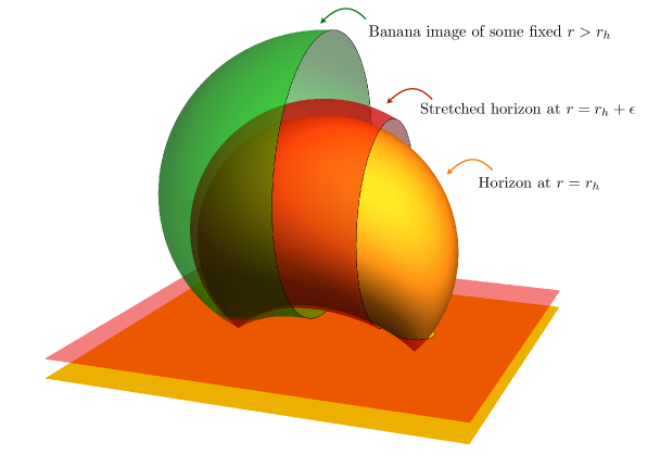
Figure 1: The banana foliation. (See also figure 3.)

For two-point function geometries, the relationship between global and Poincaré coordinates is a bit more subtle. The reason is that, unlike the case of embedded objects, the metric itself transforms in a nontrivial way. Nevertheless, we will construct a change of coordinates that maps a geometry with global asymptotics to a geometry with Poincaré asymptotics. We will call this the Global-to-Poincaré (GtP) map. The spacetime we end up with has novel features which we will describe in detail. To start with, we can picture how it looks by visualising the foliation defined by mapping surfaces of constant $r$ in global coordinates into the Poincaré picture. This foliation is composed of “spacetime bananas” that originate from the marked points, e.g., see figure 1.

The induced metric on the spacetime bananas is what characterises the backreaction of the operators inserted. For gravitational solutions which have a smooth interior, we can follow the foliation to the point where it shrinks to the geodesic connecting the two boundary points. In a neighbourhood of that geodesic, the metric depends on the specifics of the operators inserted, and it will deviate strongly from empty AdS.

When the operator insertions have created a black hole connecting the two insertion points, we can follow the foliation in figure 1 only up to the innermost banana which is the GtP image of the black hole horizon at $r=r_{h}$. As is characteristic of a black hole horizon, the induced geometry on this innermost banana maintains a finite size in the transverse directions (i.e. the horizon area) but has zero length in the longitudinal direction (i.e. the analog of the $\tau$ direction). The latter results in a conical singularity on this surface. This zero-length direction goes between the insertion points, passing through the bulk. Therefore, we have to be careful when picturing the horizon as a banana (as in figure 1), since the proper length along this banana actually vanishes. For the purpose of visualization, it is useful to think instead of a “stretched horizon", a banana that is some small distance outside of the horizon. This perspective is also closely related to the membrane paradigm [3], which constructs a simplified model to describe the black hole by replacing it with a physical surface (or membrane) at a vanishingly close distance from the event horizon.

At this point, it may beneficial for our reader if we step back to compare our approach to more traditional calculations with Euclidean black holes. First, a comment on nomenclature is that we continue to use “horizon", an intrinsically Lorentzian concept, to refer to the innermost surface in our Euclidean geometry. This is a codimension-two surface since the length along the (Euclidean) “time" direction vanishes, as noted above. Traditionally, one makes the Euclidean time direction periodic and fixes the periodicity to maintain a smooth geometry across this surface. Of course this is the starting point in using Euclidean black hole geometries to study black hole thermodynamics, e.g., [4]. In our approach, we are not enforcing any periodicity for the time coordinate. In this regard, our geometries are analogous to “fixed area" states [5, 6], which have recently appeared in discussions of quantum information aspects of holography. In either of these contexts, one is considering an ensemble of high energy states in the boundary CFT while we wish to consider a single state, i.e., the state created by the insertion of our huge operator. The latter requires that our Euclidean action includes a boundary contribution, i.e., the Gibbons-Hawking-York (GHY) term [4, 7], at a stretched horizon to fix the boundary conditions there – again, in contrast to the ensemble calculations.

The importance of the latter is also emphasized by the following holographic considerations: What we want for our geometry is that the onshell action computes a CFT two-point function, rather than say the Gibbs free energy at fixed temperature $\beta^{-1}$. Thus, our computation is more closely related to a Euclidean time translation amplitude rather than a trace over an ensemble of states with a thermal circle. Schematically,

$$\langle\text{BH}|e^{-H\delta\tau}|\text{BH}\rangle=e^{-E\delta\tau}\qquad\text{rather than}\qquad Z={\rm tr}(e^{-\beta\hat{H}})=e^{-\beta E+S}\,.$$ (1.2)

In both cases, the right-hand side is computed by the onshell action of a gravitational background, and roughly $\delta\tau\sim\log|x_{12}|^{2}$. But for a two-point function, there should be no entropy contribution! It will turn out that the GHY boundary term on the stretched horizon is crucial to remove the entropy appearing in the calculation of the thermal ensemble. Let us also note that one can interpret this new boundary term as the “membrane action" [8] within the framework of the membrane paradigm.

The remainder of our paper is organised as follows: In section 2, we describe the salient aspects of our construction. Specifically, we introduce the GtP change of coordinates and the bananas, then we discuss a version of the onshell action computation, whose immediate aim is to highlight the emergence of nontrivial spacetime dependence, and the crucial role played by the GHY boundary term at the stretched horizon. In section 3, we describe further aspects of the two-point function geometry. In particular, we verify the conformal Ward identity from the holographic stress tensor, and we revisit the onshell action computation by discussing the implications of the fact that the Fefferman-Graham coordinates only extend to a finite surface in the bulk, which we call “the wall". In section 4, we build on the idea of the horizon as a membrane by showing that – absent fine tuning – geodesics anchored at the boundary always remain outside the horizon banana. Then, we compute the action of such geodesics and show in examples that at leading order in the black hole mass, the result is simply the stress tensor conformal block. Finally, we conclude with a discussion of our results and future directions in section 5. There, we sketch an outline of our plan to extend our calculations to three- and higher-point geometries, which we will investigate in the future [1].

2 The Banana Geometry

In 1916, Schwarzschild discovered the first black hole solution of Einstein gravity. Here we will give it a new outfit, and show how it looks when we think of it as a two-point function geometry. As described in the introduction, from this new point of view, the black hole will look like a spacetime banana.

2.1 AdS-Schwarzschild

In global coordinates, the Euclidean metric of the $(d+1)$-dimensional AdS-Schwarzschild black hole reads

$$ds^{2}_{\texttt{global}}=f(r)d\tau^{2}+\frac{dr^{2}}{f(r)}+r^{2}d\Omega_{d-1}^{2}$$ (2.1)

where the blackening factor is

$$f(r)=1+r^{2}-\frac{\alpha M}{\,\,r^{d-2}}.$$ (2.2)

Here $M$ is the black hole mass (= energy) if the parameter $\alpha$ takes the canonical value,

$$\alpha=\frac{16\pi G_{\textrm{\tiny N}}}{(d-1)\Omega_{d-1}}\,,\qquad{\rm where}\quad\Omega_{d-1}=\texttt{Vol(unit (d-1)-sphere)}=\frac{2\pi^{d/2}}{\Gamma\!\left({d}/2\right)}$$ (2.3)

and $G_{\textrm{\tiny N}}$ is Newton’s constant in the $(d+1)$-dimensional bulk. In practice, we will set $\alpha=1$ to avoid cluttering our computations, and spell it out only in the final formulae. Further, we have implicitly set the AdS curvature scale to $L_{AdS}=1$.

The signature of the black hole can be changed from Euclidean to Lorentzian by taking $\tau=-it$. In either signature, the vector along the time direction is Killing and has norm square proportional to $f(r)$. This norm vanishes at the real value of $r=r_{h}$ where $f(r_{h})=0$, i.e., the Killing vector becomes null in Lorentzian signature and vanishes in Euclidean signature. This value, $r=r_{h}$, sets the location of the horizon, and it depends on $M$. Very light black holes with $M\ll 1$ have a very small horizon radius $r_{h}$, i.e. they are effectively small excitations in the middle of AdS. Very heavy black holes with $M\gg 1$ have a horizon radius scaling with $M^{1/d}$ and thus occupy most of the AdS spacetime.

Of course, in Lorentzian signature, the horizon $r=r_{h}$ is the locus where light accumulates from the point of view of an observer at infinity. Free falling observers nevertheless cross the horizon in a finite proper time. On the other hand, as discussed in the introduction, in Euclidean signature, the spacetime ends at the horizon $r=r_{h}$. There will be a conical singularity at the horizon unless Euclidean time is compactified to a circle, $\tau\sim\tau+\beta$, where the periodicity is given by the inverse Hawking temperature

$$T_{\textrm{\tiny H}}\equiv\beta^{-1}=\frac{f^{\prime}(r_{h})}{4\pi}\,.$$ (2.4)

Then, the $(\tau,r)$ geometry is that of a “cigar” ending at $r=r_{h}$ (see [9] for a nice review). The horizon area is $A=r_{h}^{d-1}\Omega_{d-1}$, and it determines the black hole entropy $S={A}/{4G_{\textrm{\tiny N}}}$ in the thermodynamic interpretation of the black hole [4].

What we want for a Euclidean two-point function geometry is a black hole connecting the insertion points at the boundary of AdS in Poincaré coordinates. This picture would match with what we expect for very light black holes behaving as structureless point particles travelling through the AdS vacuum. In that case, the two-point function would be computed by a geodesics anchored at the insertion points.

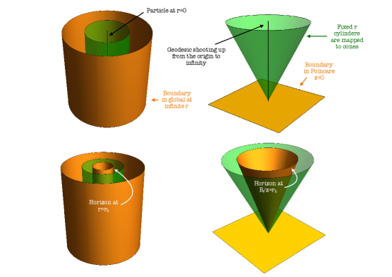
Figure 2: Global (Left) and Poincaré (Right) are related by the map in eq. (2.5). The trajectory of a particle at rest in the middle of global AdS is mapped to a geodesic shooting from the origin to infinity in Poincaré AdS, and the $\mathbb{R}\times S^{d-1}$ boundary at $r=\infty$ is mapped to the Poincaré boundary at $\tilde{z}=0$. Cylinders of varying $r$ that interpolate between the center and the boundary of global AdS correspond to cones in Poincaré coordinates. For black holes, there is an horizon at $r=r_{h}$ which corresponds to a minimal cone at $R/\tilde{z}=r_{h}$.

To match with our expectation, we look for a change of coordinates such that the center of global AdS, namely $r=0$ and $-\infty\leq\tau\leq\infty$, is mapped precisely to that geodesic in Poincaré AdS anchored at the insertion points of the two-point function. Further, we require that the $\mathbb{R}\times S^{d-1}$ boundary of global AdS is conformally mapped to the $\mathbb{R}^{d}$ boundary of Poincaré AdS. With the insertion points at $0$ and $\infty$, we can use $SO(d-1)$ invariance to restrict ourselves to $\tau=\tau(z,R)$ and $r=r(z,R)$ where $R$ is the radial coordinate in the Poincaré boundary. Then, the two conditions above are enough to suggest the change of variables

$$\tau=\frac{1}{2}\log(\tilde{z}^{2}+R^{2})\qquad;\qquad r=\frac{R}{\tilde{z}}\,.$$ (2.5)

Under this map, cylinders of constant radius in global coordinates are mapped to cones in Poincaré coordinates, and translations in global time are mapped to dilations preserving these cones – see Figure 2. We call this map the Global to Poincaré (GtP) map.

After the GtP mapping (2.5), the black hole metric takes the form

$$ds^{2}_{cone}=\frac{1}{\tilde{z}^{2}}\left[\frac{d\tilde{z}^{2}}{h(\tfrac{R}{\tilde{z}})}+h(\tfrac{R}{\tilde{z}})\left(dR+\tfrac{R}{\tilde{z}}\,v(\tfrac{R}{\tilde{z}})d\tilde{z}\right)^{2}+R^{2}d\Omega_{d-1}^{2}\right]\,,$$ (2.6)

where

$$h(r)=\frac{1}{f(r)}+\frac{r^{2}f(r)}{(1+r^{2})^{2}}\qquad{\rm and}\qquad v(r)=\frac{1}{f(r)h(r)}\left[\frac{f(r)^{2}}{(1+r^{2})^{2}}-1\right]\,.$$ (2.7)

With $M=0$, we have $f=1+r^{2}$. As a result, one finds $h=1$ and $v=0$, and the above metric (2.6) reduces to exactly Poincaré AdS.

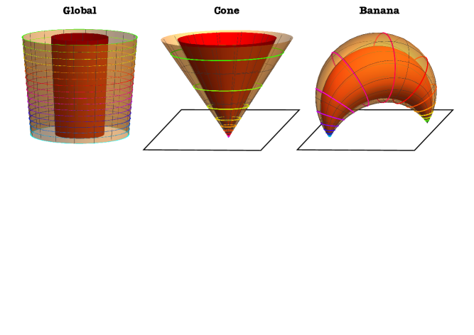
Figure 3: Black hole in global AdS (left), as a cone (middle) and a banana (right). The red corresponds to the horizon at $r=r_{h}$, while the semi-transparent surface corresponds to some constant $r$ surface with $r>r_{h}$. There is a conical singularity at the horizon, since we did not make $\tau$ periodic.

Finally, we can bring the insertion point at $\infty$ to a finite distance by a change of coordinates that acts as a special conformal transformation (SCT) on the boundary. Upon introducing Cartesian coordinates $\tilde{x}^{i}$ to replace the polar coordinates $R,\Omega_{i}$ on the boundary, desired change of coordinates in the bulk is

$$\begin{array}[]{ll}\tilde{x}^{i}&\rightarrow\displaystyle{x}^{i}=\frac{{\tilde{x}}^{i}-b^{i}\,(\tilde{x}^{2}+z^{2})}{\widetilde{\Theta}^{2}}\\ \tilde{z}&\rightarrow\displaystyle z=\frac{\tilde{z}}{\,\widetilde{\Theta}^{2}}\end{array}\qquad{\rm with}\quad\widetilde{\Theta}^{2}=1-2\,b\cdot{\tilde{x}}+b^{2}(\tilde{x}^{2}+\tilde{z}^{2})\,.$$ (2.8)

We call the above transformation the SCT mapping. It is useful to recall that the inverse of the SCT mapping with shift parameter $b^{i}$ is simply another SCT map with shift $-b^{i}$.

We denote the points at which the operators are inserted as $\vec{x}_{\bullet 1}=0$ and $\vec{x}_{\bullet 2}=-\frac{b^{i}}{b^{2}}$. Without loss of generality, we can choose $\vec{x}_{\bullet 1}-\vec{x}_{\bullet 2}$ to lie along the ${x}^{1}$-axis, i.e., $b^{i}=b\,\delta^{i1}$. Then the geometry maintains a rotational $SO(d-2)$ symmetry in the remaining Cartesian directions. If we denote the radius in these transverse directions as $\rho=(\sum_{i=2}^{d}({x}^{i})^{2})^{1/2}$, then the metric takes the form

$$ds^{2}_{banana}=N_{z}^{2}\,dz^{2}+\sum_{a,b={x}^{1},\,\rho}h_{ab}(dy^{a}+N^{a}_{z}\,dz)(dy^{b}+N^{b}_{z}\,dz)+\frac{\rho^{2}\,d\Omega_{d-2}^{2}}{z^{2}}$$ (2.9)

The explicit form of the components is not very illuminating, and hence we omit them here. Of course, the symmetry is enhanced to $SO(d-1)$ with $b\to 0$, since the cone metric (2.6) is recovered in this limit.

In figure 3, we illustrate the various coordinate transformations. Upon performing the SCT map, the foliation by cones (with $b=0$) becomes a foliation by bananas (with $b\neq 0$). More precisely, each constant $r$ cylinder in global coordinates is mapped to the banana

$$r^{2}=\Theta^{2}\left(\frac{x^{2}}{z^{2}}+1\right)-1\qquad{\rm with}\quad\Theta^{2}=1+2\,b\cdot{x}+b^{2}(x^{2}+z^{2})$$ (2.10)

Solving this equation for $z$ gives two positive components $z_{\pm}(r)\geq 0$, distinguished by the sign of a square root – see figure 4 and also eq. (2.19). The $z_{-}$ component has the shape of a pair of pants, while the $z_{+}$ component is a cap. In the limit $b\to 0$, the former transitions to the cone surfaces and $z_{+}$ goes off to infinity.

Of course, the induced metric on each banana is the same as that of a surface of constant $r$ in global coordinates, even if the metric looks initially more complicated. For example, restricting to a cone $\tilde{z}=\frac{R}{r}$ with a fixed value $r\in\mathbb{R}$ in eq. (2.6), a direct computation yields

$$ds^{2}_{\tt cone}\big{|}_{\tilde{z}=\frac{R}{r}}=f(r)\,\frac{dR^{2}}{R^{2}}+r^{2}d\Omega_{d-1}^{2}\,.$$ (2.11)

Further, eq. (2.5) yields $\frac{dR}{R}=d\tau$ with fixed $r$, and hence eq. (2.11) reduces to precisely the same induced metric as in global coordinates (2.1) with fixed $r$.

Although the induced metric on the bananas is the same as in global coordinates, the main purpose of the GtP map is to give us a Poincaré boundary, which allows us to study the backreaction of the operators along slices of constant $z$, i.e., the bulk evolution picture. The surface $z=\epsilon$ is also a simple cut-off surface for computing the onshell action, which is ultimately what we want to compute to match with a CFT two-point function. The main novelty here is that the $z=\epsilon$ surface contains points which are both far and close to the operator insertions, i.e., far and close to the black hole horizon. Thus the pre-image of $z=\epsilon$ in global coordinates is a surface that explores the space from near the asymptotic boundary to deep into the bulk, and therefore the corresponding boundary conditions probes properties of the geometry that are usually viewed as distinct, i.e., near infinity and in the interior. While this distinction will be formalised in section 3 where we discuss the Fefferman-Graham patch, we first need to understand how to deal with the horizon.

As mentioned in the introduction, traditionally Euclidean black holes appear as the bulk saddle point describing a n ensemble of high energy states in the boundary CFT. In contrast, we wish to consider a single unique state, i.e., the state created by the insertion of our huge operator. For this purpose, we introduce a stretched horizon at $r=r_{h}(1+\epsilon^{\prime})$. away from the horizon. Then to fix the boundary conditions at the horizon, we introduce Gibbons-Hawking-York (GHY) term [4, 7] on the stretched horizon and then take the limit $\epsilon^{\prime}\to 0$.

In sum, the total onshell action for our two-point function black hole is

$$I_{\leavevmode\hbox to14.63pt{\vbox to8.94pt{\text{[drawing]}}}}=I_{bulk}\ +\ I_{boundary}\ +\ I_{ct}$$ (2.12)

where the first term is the Einstein-Hilbert bulk action (with a negative cosmological constant). The boundary action is comprised of two GHY terms, one on the asymptotic boundary and the other on the stretched horizon, i.e.,

$$I_{boundary}=I_{GHY}(\partial_{AdS})+I_{GHY}({\rm stretch})\,.$$ (2.13)

Finally, there are the boundary counterterms $I_{ct}$ which are evaluated on the asymptotic boundary, e.g., see [10, 11, 12, 13, 14, 15]. In the next section, we discuss the precise definition of all of these terms $I_{bulk},\ I_{boundary}$ and $I_{ct}$, and further we will compute their values.

2.2 CFT two-point function from gravity: the onshell action

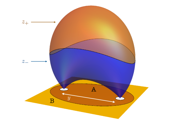
Figure 4: The two solutions $z_{\pm}$ of the banana equation (2.10). We denote the (boundary) distance between the insertion points as $|\vec{x}_{\bullet 1}-\vec{x}_{\bullet 2}|=y=\frac{1}{b}$. The $z_{-}$ component has the shape of a pair of pants, while $z_{+}$ is a cap. For $r=r_{h}$, we denote the inside and outside of the ellipse below the stretched horizon as $A$ and $B$, respectively.

The goal of this section is to evaluate the gravitational action $I_{\leavevmode\hbox to14.63pt{\vbox to8.94pt{\text{[drawing]}}}}$ for the banana geometry and show that it reproduces a scalar two-point CFT correlator. Of course, given eq. (1.1), we know what to expect:

$$I_{\leavevmode\hbox to14.63pt{\vbox to8.94pt{\text{[drawing]}}}}=\Delta\,\log\!|\vec{x}_{\bullet 1}-\vec{x}_{\bullet 2}|^{2}\,+\,\texttt{distance-independent\,constant}$$ (2.14)

so that

$$\langle O(\vec{x}_{\bullet 1})O(\vec{x}_{\bullet 2})\rangle=e^{-I_{\leavevmode\hbox to14.63pt{\vbox to8.94pt{\text{[drawing]}}}}}\simeq\frac{1}{|\vec{x}_{\bullet 1}-\vec{x}_{\bullet 2}|^{2\Delta}}\,.$$ (2.15)

We will focus first on reproducing the spacetime dependence as function of $\Delta$. We will also comment on the overall normalisation, which was omitted in eq. (2.15).

As pointed out already in (2.12), there are three contributions to the total action, which come from: bulk, boundaries and counterterms,

$$I_{\leavevmode\hbox to14.63pt{\vbox to8.94pt{\text{[drawing]}}}}=I_{bulk}\ +I_{GHY}(\partial_{AdS})+I_{GHY}({\rm stretch})+\ I_{ct}$$ (2.16)

We will analyse each of them in turn.

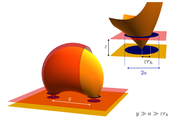
Figure 5: To regulate the onshell action, we introduce a cut-off surface at $z=\epsilon$ near the asymptotic boundary and a stretched horizon at $r=r_{h}(1+\epsilon^{\prime})$. These two surfaces intersect and effectively excise a disk of radius $r_{h}\epsilon$ to leading order in $\epsilon$, close to the insertion points. To compute the boundary integrals, we will excise a larger disk of radius $a$, much smaller than the separation between the insertions $y=\frac{1}{b}$, but much larger than $\epsilon r_{h}$. We will show that this scheme reproduces the expected spacetime dependence $y^{-2\Delta}$ of a two-point function, up to a distance-independent constant. .

2.2.1 The bulk action

The Einstein-Hilbert action is

$$I_{bulk}=-\frac{1}{16\pi G_{\textrm{\tiny N}}}\int\!d^{d}x\,dz\,\sqrt{g}\left(R+\frac{d(d-1)}{L_{AdS}^{2}}\right)\,.$$ (2.17)

Here and below, we are implicitly working with the metric (2.9) using the coordinates introduced by the SCT mapping (2.8). Then upon using the Einstein equations and carrying out the $dz$ integration for $z\geq\epsilon$, we find

$$I_{bulk}=\frac{1}{8\pi G_{\textrm{\tiny N}}}\int_{A}\!d^{d}x\left[\frac{1}{z_{+}(r_{h})^{d}}-\frac{1}{z_{-}(r_{h})^{d}}\right]+\frac{1}{8\pi G_{\textrm{\tiny N}}}\int_{A\cup B}\!\!d^{d}x\ \frac{1}{\epsilon^{d}}$$ (2.18)

where the domain of integration $A$ is the ellipse given by projecting the banana describing the horizon into the boundary coordinates – see figure 4 and eq. (2.20). $B$ is the domain outside this ellipse and hence, the second term, which is the usual divergence of the $AdS$ volume, is integrated over the entire AdS boundary.

The first term consists of the boundary contributions coming from where the $z$ integration reaches the banana at the (stretched) horizon, and $z_{\pm}(r_{h})$ are the two components of this banana described below eq. (2.10). Substituting $r=r_{h}$ into eq. (2.10), we find

$$z_{\pm}(r_{h})=\Bigg{[}\tfrac{r_{h}^{2}}{2b^{2}}-x^{1}\left(x^{1}+\tfrac{1}{b}\right)-\rho^{2}\pm\frac{r_{h}}{b}\,\sqrt{\tfrac{r_{h}^{2}}{4b^{2}}-x^{1}\left(x^{1}+\tfrac{1}{b}\right)-\rho^{2}\left(1+\tfrac{1}{r_{h}^{2}}\right)}\Bigg{]}^{\frac{1}{2}}\,,$$ (2.19)

as depicted in figure 4. The ellipse dividing the domains $A$ and $B$ corresponds to the vanishing locus of the square root in the above expression. Hence A is given by the inequality,

$$x^{1}\left(x^{1}+\tfrac{1}{b}\right)+\rho^{2}\left(1+\tfrac{1}{r_{h}^{2}}\right)\leq\tfrac{r_{h}^{2}}{4b^{2}}$$ (2.20)

where as discussed below eq. (2.8), we have placed the two insertion points on the $x^{1}$-axis at $x^{1}=0$ and $-1/b$.

The bulk construction with the stretched horizon implies that we should also excise a small disk around each insertion point from the inner domain $A$ for the term involving $z_{-}(r_{h})$ – see figure 5. As we shall see, this feature of the computation is precisely the reason why the first contribution in eq. (2.18) is nonstandard and interesting to evaluate.

Let us examine how the $z_{-}$ component reaches the insertion points, by zooming there with a small $\delta$ expansion, $(x^{1},\rho)\rightarrow\delta\,(x^{1},\rho)$ and $(x^{1},\rho)\rightarrow(-\frac{1}{b},0)+\delta\,(x^{1},\rho)$. We find

$$\frac{1}{z_{-}(r_{h})^{d}}=r_{h}^{d}\,\underbrace{\frac{1}{((x^{1})^{2}+\rho^{2})^{d/2}\,((1+bx^{1})^{2}+b^{2}\rho^{2})^{{d}/{2}}}}_{f_{2pt}}\,+\,{\cal D}(x_{1},x_{2},r_{h};b)$$ (2.21)

where the difference function $\cal{D}$ vanishes when $b=0$. The first term in its most general form is given by

$$f_{2pt}=\frac{|\vec{x}_{\bullet 1}-\vec{x}_{\bullet 2}|^{d}}{|\vec{x}-\vec{x}_{\bullet 1}|^{d}\,|\vec{x}-\vec{x}_{\bullet 2}|^{d}}.$$ (2.22)

i.e., a simple function of distances. The integral of $f_{2pt}$ in $A$ diverges logarithmically, while instead the reminder ${\cal D}$ is integrable in $A$. On the other hand, $f_{2pt}$ is integrable at infinity, and thus in $B$. Therefore, by adding and subtracting $f_{2pt}$ in $B$, we can write the bulk action as

$$I_{bulk}= \frac{1}{8\pi G_{\textrm{\tiny N}}}\int_{A\cup B}\!\!d^{d}x\ \bigg{[}\frac{1}{\epsilon^{d}}-r_{h}^{d}\,f_{2pt}(x)\bigg{]}+{\cal N}_{bulk}$$ (2.23)

where we defined the constant

$${\cal N}_{bulk}=\frac{1}{8\pi G_{\textrm{\tiny N}}}\int_{B}d^{d}x\ r_{h}^{d}\,f_{2pt}+\frac{1}{8\pi G_{\textrm{\tiny N}}}\int_{A}d^{d}x\bigg{[}\frac{1}{z_{+}(r_{h})^{d}}-{\cal D}\bigg{]}\,.$$ (2.24)

We emphasize that ${\cal N}_{bulk}$ is a constant independent of the seperation $|\vec{x}_{\bullet 1}-\vec{x}_{\bullet 2}|=1/b$. Indeed, if we rescale the coordinates, say $(x^{1},\rho)\rightarrow(x^{1}/b,\rho/b)$, the dependence on the separation factors out completely from $z_{\pm}$ in eq. (2.19) and from $f_{2pt}$ and ${\cal D}$ in eq. (2.21). Further, this overall factor cancels precisely that coming from the measure $d^{d}x$ in the two integrals comprising ${\cal N}_{bulk}$ in eq. (2.24). Similarly, the $b$ dependence also scales out of the ellipse separating $A$ and $B$, e.g., see eq. (2.20). Finally, since there is no divergence in ${\cal D}$ near the insertion points, we can close the disks opened in $A$. Hence we conclude that ${\cal N}_{bulk}$ is completely independent of the separation between insertion points, and in fact eq. (2.24) yields a finite constant depending only on $r_{h}$ in the $\epsilon\rightarrow 0$ limit.

The contribution coming from the first term in eq. (2.23) is different because $f_{2pt}$ yields a logarithmic divergence, and so it is really crucial to excise a disk of radius $a$ around each of the insertion points. Thus, although the dependence on $|\vec{x}_{\bullet 1}-\vec{x}_{\bullet 2}|$ can be scaled away between the integrand and the measure, as above, this rescaling changes the domain of integration. Hence the integral does depend on the distance.

2.2.2 The asymptotic boundary action

The action has two contributions on the asymptotic AdS boundary. The first is the GHY term

$$I_{GHY}(\partial_{AdS})=\frac{1}{8\pi G_{\textrm{\tiny N}}}\int_{\partial}d^{d}x\sqrt{h}\,{K}_{\partial_{AdS}}\qquad{\rm with}\quad{K}_{\partial_{AdS}}=-\nabla_{\mu}\frac{N_{z}^{\mu}}{|N_{z}|}$$ (2.25)

and the second, the counterterm action

$$I_{ct}=\frac{1}{8\pi G_{\textrm{\tiny N}}}\int_{\partial}\!\!d^{d}{x}\,\sqrt{h}\,\Bigg{(}(d-1)+\frac{1}{2(d-2)}\,{\cal R}[h]+\cdots\Bigg{)}\,.$$ (2.26)

Here we are using the boundary metric $h_{ij}$ at $z=\epsilon$ and the outward-pointing unit normal vector $N_{z}^{\mu}=(-1,N_{z}^{i})$ in the banana metric. The quantities $N_{z}^{i}$ here and $N_{z}$ in eq. (2.25) correspond to those appearing in the metric (2.9).

As already mentioned, we find points that are both far and close to the horizon on the $z=\epsilon$ cut-off. For example, in the cone coordinates (2.6), on the cut-off surface $z=\epsilon$, we can approach $R=r_{h}\epsilon$ where the blackening factor vanishes, or we can consider large $R$ where the metric is Poincaré AdS at leading order in $\epsilon$. The behavior of the metric $h_{ij}$ as $\epsilon\rightarrow 0$, as well as that of $N_{z}^{i}$, depends on this distinction. To properly disentangle these two regions, we introduce Fefferman-Graham coordinates in section 3, and here we adopt a simpler strategy instead. Our approach is to choose the radius $a$ of the disks that we excise from $A$ so that the expansion of $h_{ij}$ and $N^{i}_{z}$, in $z=\epsilon$ with $\vec{x}$ fixed, is valid. This is illustrated in figure 5.

Given the approximation $|\vec{x}_{\bullet 1}-\vec{x}_{\bullet 2}|\gg a\gg\epsilon r_{h}$, the various quantities entering $I_{GHY}$ and $I_{ct}$ automatically have an expansion in $z\big{/}|\vec{x}-\vec{x}_{\bullet 1}||\vec{x}-\vec{x}_{\bullet 2}|$ because this is the expansion of the SCT map, when we go from the expansion in $z/R$ of the cone to the banana coordinates. For example, we find

$$d^{d}x\sqrt{h}=\frac{1}{z^{d}}\bigg{[}1-\frac{\alpha M}{2}\frac{z^{d}}{((x^{1})^{2}+\rho^{2})^{\frac{d}{2}}((1+bx^{1})^{2}+b^{2}\rho^{2})^{\frac{d}{2}}}+\ldots\bigg{]}dx^{1}\rho^{d-2}d\rho\,d\Omega_{d-2}$$ (2.27)

Then, at leading order $K_{\partial_{AdS}}=-d+O(z^{d+1})$ and the counterterms involving the boundary curvature are suppressed because of the flat metric on the asymptotic boundary. Combining the asymptotic boundary contributions with the bulk action (2.23), we find

$$I_{bulk}+I_{GHY}(\partial_{AdS})+I_{ct}\simeq\frac{(\alpha M-2r_{h}^{d})}{16\pi G_{\textrm{\tiny N}}}\int_{\leavevmode\hbox to14.63pt{\vbox to8.94pt{\text{[drawing]}}}}\!\!\!d^{d}{x}\,f_{2pt}\,,$$ (2.28)

up to the constant term ${\cal N}_{bulk}$. The domain of integration is the entire boundary minus the small disks around the insertion points, which we denote $\leavevmode\hbox to14.63pt{\vbox to8.94pt{\text{[drawing]}}}=A\cup B-{\rm disks}$.

The integral of $f_{2pt}$ can be performed by introducing bipolar coordinates. Let us simply quote the final result,

$$\int_{\leavevmode\hbox to14.63pt{\vbox to8.94pt{\text{[drawing]}}}}\!\!\!d^{d}{x}\,f_{2pt}=\Omega_{d-1}\log\frac{|\vec{x}_{\bullet 1}-\vec{x}_{\bullet 2}|^{2}}{a^{2}}$$ (2.29)

The overall coefficient in eq. (2.28) then becomes

$$\frac{\Omega_{d-1}}{16\pi G_{\textrm{\tiny N}}}\,\left(\alpha M-2r_{h}^{d}\right)=M-S\,T_{H}=F_{\textrm{\tiny Gibbs}}$$ (2.30)

where

$$E=\frac{\Omega_{d-1}(d-1)\alpha M}{16\pi G_{\textrm{\tiny N}}}=M\,,\qquad\quad S=\frac{\Omega_{d-1}r_{h}^{d-1}}{4G_{\textrm{\tiny N}}}\,,\qquad\quad T_{H}=\frac{f^{\prime}(r_{h})}{4\pi}$$ (2.31)

with the blackening factor $f(r)$ and the coefficient $\alpha$ given in eqs. (2.2) and (2.3), respectively. Therefore,

$$I_{bulk}+I_{GHY}(\partial_{AdS})+I_{ct}=(M-S\,T_{H})\,\log\frac{|\vec{x}_{\bullet 1}-\vec{x}_{\bullet 2}|^{2}}{a^{2}}+{\cal N}_{bulk}\,.$$ (2.32)

We have nearly reproduced the desired CFT spacetime dependence, since we have a logarithm coming from $f_{2pt}$. However, the prefactor for this logarithm is the Gibbs free energy, similarly to what we would have expected had we done the computation in global AdS – but for a possible Casimir energy. However, as discussed in eq. (2.14), we expect the prefactor to the CFT dimension $\Delta=M$. That is, we would like to subtract the entropy contribution in eq. (2.32). In the following subsection, we will see that the GHY contribution on the stretched horizon does precisely this. This confirms that this surface term is precisely what is needed to fix the calculation to that of a single operator inserted at the asymptotic AdS boundary.

2.2.3 The stretched horizon action

Recall that we introduced a final boundary at the stretched horizon $r=r_{h}(1+\epsilon^{\prime})$ and supplemented the action with a GHY term there, namely

$$I_{GHY}({\rm stretch})=\frac{1}{8\pi G_{\textrm{\tiny N}}}\int_{\partial}d^{d}x\lim_{\epsilon^{\prime}\rightarrow 0}\sqrt{\sigma}\,K_{\textrm{\tiny stretch}}\qquad{\rm with}\quad K_{\textrm{\tiny stretch}}=-\nabla_{\mu}\frac{V^{\mu}}{|V|\,}$$ (2.33)

where the extrinsic curvature $K$ is now determined by the divergence of a vector $V^{\mu}$ orthogonal to the stretched horizon, and $\sigma$ is the determinant of the induced metric on the stretched horizon.

We can find $V^{\mu}$ by considering the image of $\partial_{r}$ through the GtP and SCT transformations. This gives

$$\frac{V_{\mu}}{|V|\,}=-\frac{1}{\sqrt{f(r)}}\,\partial_{\mu}r(\vec{x},z)$$ (2.34)

where $r(\vec{x},z)$ in eq. (2.10). Simplifying the divergence as in footnote 12, and further using $f(r_{h})=0$ with $f^{\prime}(r_{h})=4\pi T_{H}$, we arrive at

$$K_{\textrm{\tiny stretch}}=\frac{2\pi T_{H}}{\sqrt{f(r)}}\,.$$ (2.35)

On the other hand, if we only had the banana metric (2.9) (i.e., we did not know the transformations from the global coordinates and the relation $r_{h}=r(z,\vec{x})$), we could obtain the same result by looking at the vector orthogonal to the Killing flow in $(\vec{x},z)$ coordinates to construct $V^{\mu}$.

To complete $I_{GHY}({\rm stretch})$, we need to compute the determinant of the induced metric, which we find takes the form

$$d^{d}x\,\sqrt{\sigma}=\frac{\rho^{d-2}\,d\Omega_{d-1}}{z^{d-2}}\,\frac{\sqrt{f(r)}dx^{1}\,d\rho}{z^{2}r_{h}}\times\bigg{(}1+\tilde{\cal D}(x_{1},x_{2},r_{h};b)\bigg{)}\Bigg{|}_{z=z_{\pm}}$$ (2.36)

where the difference function $\tilde{\cal D}$ vanishes exactly for $b=0$, and for $b\neq 0$ vanishes linearly when we expand around the insertion points. As we did before, we now specialize to the $z=z_{-}$ component of the stretched horizon, and extract the logarithmic form. This is again singled out by $z_{-}^{d}$ in the denominator of eq. (2.36), which similarly to eq. (2.21) leads to $r_{h}^{d}\,f_{2pt}$ in the domain $A$. The overall power of $r_{h}$ is then $r_{h}^{d-1}=4G_{\textrm{\tiny N}}\,S/\Omega_{d-1}$. Finally, by adding and subtracting $f_{2pt}$, we conclude that

$$I_{GHY}({\rm stretch})=S\,T_{H}\,\log\frac{|\vec{x}_{\bullet 1}-\vec{x}_{\bullet 2}|^{2}}{a^{2}}+{\cal N}_{\textrm{\tiny stretch}}\,.$$ (2.37)

With the same argument as for ${\cal N}_{bulk}$. we can show that ${\cal N}_{\textrm{\tiny stretch}}$ is a constant that does not dependent on the separation between insertion points.

2.2.4 CFT from gravity

Combining eqs. (2.32) and (2.37) for the total onshell action, our final result reads

$$I_{\leavevmode\hbox to14.63pt{\vbox to8.94pt{\text{[drawing]}}}}=M\log\frac{|\vec{x}_{\bullet 1}-\vec{x}_{\bullet 2}|^{2}}{a^{2}}+{\cal N}$$ (2.38)

where $M=\Delta$ and ${\cal N}={\cal N}_{bulk}+{\cal N}_{\textrm{\tiny stretch}}$. It follows that

$$\langle O(\vec{x}_{\bullet 1})O(\vec{x}_{\bullet 2})\rangle=e^{-I_{\leavevmode\hbox to14.63pt{\vbox to8.94pt{\text{[drawing]}}}}}\simeq\frac{1}{|\vec{x}_{\bullet 1}-\vec{x}_{\bullet 2}|^{2\Delta}}\,,$$ (2.39)

as promised. In sum, taking into account the backreaction from the insertion of two huge operators, the gravitational action, including a GHY term at the horizon, yields to the desired CFT two-point function (2.15).

A posteriori, we find that the onshell action in the two-point function geometry gives a result which is consistent with the following sequence of operations,

$$Z={\rm tr}(e^{-\beta\hat{H}})=e^{-\beta F_{\textrm{\tiny Gibbs}}}\ \rightarrow e^{-F_{\textrm{\tiny Gibbs}}\delta\tau}\rightarrow e^{-E\delta\tau}\rightarrow e^{-\Delta\delta\tau}\,.$$ (2.40)

Starting from the thermal partition function, which computes $F_{\textrm{\tiny Gibbs}}=E-S\,T_{H}$, we open up the thermal circle $\beta$ to an interval of length $\delta\tau$. This gives $e^{-F_{\textrm{\tiny Gibbs}}\delta\tau}$ where now the endpoints play the role of the operator insertions, and induce a conical singularity in the bulk. To account for the latter, we include the GHY term at the stretched horizon, and this changes $F_{\textrm{\tiny Gibbs}}$ into $E$. Up to this point, the CFT has $S^{d-1}$ as its spacial slice and $E$ includes also Casimir energies in even $d$. By performing a Weyl transformation, we put the CFT on $\mathbb{R}^{d}$. This changes the AdS cut-off and yields the final “dilatation amplitude”, $e^{-\Delta\delta\tau}$. The actual computation which we performed shows how the $\log|\vec{x}_{\bullet 1}-\vec{x}_{\bullet 2}|$ dependence comes about and in particular the importance of excising small disks around the operators.

We also have the normalization $\mathcal{N}$. It can be written down by following carefully the various steps above. Still, on its own it can always be absorbed in the definition of the operator. Physical quantities involve ratios, such as three-point couplings divided by two-point function normalizations. Then it is crucial to make sure that once we attack higher-point correlation functions, we compute them with the same scheme we are using for the two-point function. This is one of the motivations for the explorations that follow.

3 Fefferman-Graham Coordinates

In this section, we explore further aspects of the banana geometry. In particular, we will introduce Fefferman-Graham coordinates, verify that the holographic stress tensor satisfies the conformal Ward Identity, and discuss a nonperturbative feature of the Fefferman-Graham patch, which we call the wall. With these insights, we will then revisit the notion of the cut-off surface at the boundary of AdS with marked points, and the computation of the onshell action as a proper surface integral.

Let us begin by recalling that Fefferman-Graham (FG) coordinates are defined by [17, 18]

$$ds^{2}_{FG}=\frac{d{\bf z}^{2}}{{\bf z}^{2}}+{\bf h}_{ij}({\bf z},\vec{\bf x})\,d{\bf x}^{i}\,d{\bf x}^{j}\,.$$ (3.1)

The banana metric (2.9) is not in this gauge, but can be brought to this form by a change of variables $z=z({\bf z},\vec{\bf x}),\,x^{i}=x^{i}({\bf z},\vec{\bf x})$, which is uniquely specified by requiring absence of mixed terms $d{{\bf z}}\,d\vec{\bf x}$ and that $g_{{\bf z}{\bf z}}=1/{\bf z}^{2}$ is fixed. In this gauge, ${\bf h}_{ij}({\bf z},\vec{\bf x})$ provides neatly the holographic evolution of the boundary metric, where the latter is defined as the leading non-normalisable mode in the small ${\bf z}$ expansion. In our case, since we are studying a vacuum solution with a flat Poincaré boundary, we will have

$${\bf h}_{ij}=\frac{1}{{\bf z}^{2}}\left(\delta_{ij}+\frac{2}{d}\,{\bf t}_{ij}\,{\bf z}^{d}+\cdots\right)$$ (3.2)

with ${\bf t}_{ij}$ traceless. Higher order terms are fixed once ${\bf t}_{ij}$ is given. Standard holographic renormalization methods, e.g., [11, 12] show that ${\bf t}_{ij}$ is the (expectation value of the) stress tensor in the boundary CFT.

In order to generate FG coordinates, we can start from the small ${\bf z}$ expansion. For the banana on the line (2.9), the FG gauge takes the form

$$ds^{2}_{FG}=\frac{d{\bf z}^{2}}{{\bf z}^{2}}+\sum_{a,b={\bf x}^{1},\,{\boldsymbol{\rho}}}{\bf h}_{ab}d{{\bf y}}^{a}d{{\bf y}}^{b}+{\bf h}_{\Omega\Omega}d\Omega^{2}_{d-2}$$ (3.3)

with metric components depending on the three variables ${\bf z},\,{\bf x}^{1}$ and ${\boldsymbol{\rho}}=(\sum_{i=2}^{d}({{\bf x}}^{i})^{2})^{1/2}$, in addition to $M$ and $b$. Resumming in three-variables is a hard problem, in general. An exception is $AdS_{3}$ where the series truncates, and we rediscover a result from Bañados [19]

$$ds^{2} = {d{\rm AdS}_{3}}^{2}+\bigg{[}{\bf t}\,(d{\bf y}^{1}+id{\bf y}^{2})^{2}+{\rm c.c.}\bigg{]}+{\bf z}^{2}\,|{\bf t}|^{2}((d{\bf y}^{1})^{2}+(d{\bf y}^{2})^{2})$$

$${\rm where}\qquad{\bf t}=-\frac{M}{4({{\bf y}}^{1}+i{{\bf y}}^{2})(1+b({{\bf y}}^{1}+i{{\bf y}}^{2}))}\,.$$

In the special case of the cone, $b=0$, the coordinates ${\bf x}^{1}$ and ${\boldsymbol{\rho}}$ combine together to restore $SO(d-1)$ symmetry, and this allows us to find

$$ds^{2}_{FG}=\frac{1}{{\bf z}^{2}}\left[d{\bf z}^{2}+\frac{(1-\frac{M{\bf z}^{d}}{4{\bf R}^{d}})^{2}}{(1+\frac{M{\bf z}^{d}}{4{\bf R}^{d}})^{\frac{2(d-2)}{d}}}d{\bf R}^{2}+(1+\tfrac{M{\bf z}^{d}}{4{\bf R}^{d}})^{\frac{4}{d}}{\bf R}^{2}d\Omega^{2}_{d-1}\right]$$ (3.5)

with the change of variables from GtP cone to FG cone given by

$$\frac{R}{z}=\frac{\bf R}{\bf z}\left(1+\frac{M}{4}\frac{{\bf z}^{d}}{{\bf R}^{d}}\right)^{\!\!\!\frac{2}{d}}\qquad;\qquad R^{2}+z^{2}={\bf R}^{2}\exp\Bigg{[}\int_{0}^{\frac{\bf z}{\bf R}}\frac{2xdx}{k(x)}\Bigg{]}$$ (3.6)

where $k(x)=x^{2}+{(1-\frac{M}{4}x^{d})^{2}}\big{/}{(1+\frac{M}{4}x^{d})^{\frac{2(d-2)}{d}}}$.

For the FG cone, $SO(d-1)$ symmetry implies that the image of a cylinder of radius $r=R/z$ in global, is again a cone. However, the FG banana looks different. For example, in AdS₃ and AdS₅, we have

$$r^{2}_{AdS_{3}}\!= \frac{\tilde{\bf R}^{2}}{{\bf z}^{2}}+\frac{M}{2}+\frac{M}{4}\bigg{[}\frac{2b({{\bf x}}^{1}(1+b{\bf x}^{1})-b{\boldsymbol{\rho}}^{2}){\bf z}^{2}}{{\bf R}^{2}{\bf R}_{b}^{2}}+\frac{M{\bf z}^{2}}{4{\bf R}^{2}{\bf R}_{b}^{2}}\bigg{]}$$ (3.7)

$$r^{2}_{AdS_{5}}\!= \frac{\tilde{\bf R}^{2}}{{\bf z}^{2}}+\frac{M{\bf z}^{2}}{4{\bf R}^{2}{\bf R}_{b}^{2}}-\frac{M}{2}\bigg{[}1-\frac{b\,{\bf z}^{2}(\tilde{\bf x}^{1}-b\,{\bf z}^{2})}{{\bf R}^{2}{\bf R}_{b}^{2}}-\frac{(\tilde{\bf R}^{2}-2b\,\tilde{\bf x}^{1}\,{\bf z}^{2})}{b\,{\boldsymbol{\rho}}\,{\bf z}^{2}}{\tan}^{-1}\bigg{[}\frac{b\,{\boldsymbol{\rho}}\,{\bf z}^{2}}{\tilde{\bf R}^{2}-b\,\tilde{\bf x}^{1}\,{\bf z}^{2}}\bigg{]}\bigg{]}+O(M^{2})$$

where $\tilde{\bf R}^{2}=(\tilde{\bf x}^{1})^{2}+{\boldsymbol{\rho}}^{2}$ with $\tilde{\bf x}^{1}={\bf x}^{1}+b\,({\bf R}^{2}+{\bf z}^{2})$, ${\bf R}^{2}=({\bf x}^{1})^{2}+{\boldsymbol{\rho}}^{2}$ and ${\bf R}_{b}^{2}=(1+b{\bf x}^{1})^{2}+b^{2}\,{\boldsymbol{\rho}}^{2}$.

The functional differences between a FG banana and a GtP banana (2.10) have a simple explanation: The GtP transformation is designed to foliate empty AdS, and knows nothing about the actual black hole metric. For example, it is $M$ independent. On the other hand, FG coordinates by construction are sensitive to the black hole geometry, thus foliate the space accordingly. There is however a limitation: the FG patch is not expected to cover the entire black hole geometry. This statement is simple to understand: since the small ${\bf z}$ expansion is fully determined by the knowledge of the boundary metric and boundary stress tensor ${\bf t}_{ij}$, there is no freedom left to impose other boundary conditions, such as regularity conditions at the horizon. This means that the FG patch must breakdown at some surface where the Jacobian of the coordinate transformation from global to FG vanishes. We will refer to this surface as the wall. In practise, the wall encloses the horizon at a finite distance, and there is no way to access the horizon from the FG patch (on a real slice).

In ${\bf x},{\bf z}$ coordinates, the wall coincides with the surface where $\det{\bf h}_{ab}=0$. This can be seen by examining the measure for the FG metric (3.3),

$$\frac{\sqrt{{\bf h}}}{\bf\ z}=\sqrt{g({\vec{\bf x},{\bf z}})\,{\rm Jac}^{2}(\vec{\bf x},{\bf z})}$$ (3.8)

and further we have $g({\vec{\bf x},{\bf z}})=\sqrt{g(r)}=r^{d-1}>0$ for the black hole metric (2.1). In the FG cone coordinates, the wall is itself a cone given by

$${\bf R}=\left(\frac{M}{4}\right)^{\!\!\frac{1}{d}}\,{\bf z}$$ (3.9)

corresponding to $r_{wall}=M^{\frac{1}{d}}$. As expected, $r_{wall}>r_{h}$. Note however that in general, the wall does not have to be a FG banana, nor the minimum in ${\bf z}$ of $r(\vec{{\bf x}},{\bf z})$ for fixed $\vec{\bf x}$. For example in AdS₃, the wall is given by

$$\left(({\bf x}^{1})^{2}+{\boldsymbol{\rho}}^{2}\right)\left((1+b{\bf x}^{1})^{2}+{\boldsymbol{\rho}}^{2}\right)=\frac{M}{4}\,{\bf z}^{2}\,,$$ (3.10)

which is not comparable with eq. (3.7).

Even so, the wall and GtP bananas both originate from the insertion points at the AdS boundary, where ${\bf z}=z=0$ and $\vec{\bf x}=\vec{x}$. The novelty is what happens with respect to the cut-off, ${\bf z}={\boldsymbol{\epsilon}}$ versus $z=\epsilon$. In fact, when we look at ${\bf z}={\boldsymbol{\epsilon}}$ in the two-point function geometry with coordinates $z,\vec{x}$, this surface cannot get arbitrarily close to the horizon, but intersects and stops at the preimage of the wall. This intersection is well defined and brings us to an important consideration: Imagine we want to construct a black hole numerically, in global coordinates. We are used to specify a boundary condition at infinity and a boundary condition in the interior. However, in the two-point function geometry, all of the boundary conditions are specified on $z=\epsilon$, and of course, they are distinct depending on whether we stay far or close to the operators. This distinction is quantified by the wall between the FG patch and the rest of the geometry. In this sense, the usual notion of bulk evolution is modified in an interesting way.

3.1 Holographic stress tensor

To compute expectation values in the holographic CFT, the small ${\bf z}$ expansion of the FG metric is all we need, and this is straightforward to obtain in even the banana geometry. The computation of the holographic stress tensors that follows is an example. Nicely enough, for the cone coordinates, we can check all the various steps directly with pencil and paper.

Using the definition of the holographic stress tensor given in [11, 12], we have

$$\langle T_{ij}(\vec{\bf x})\rangle_{\leavevmode\hbox to14.63pt{\vbox to8.94pt{\text{[drawing]}}}}=\frac{1}{8\pi G_{\textrm{\tiny N}}}\,\lim_{{\boldsymbol{\epsilon}}\rightarrow 0}\,\frac{1}{{\boldsymbol{\epsilon}}^{d-2}}\bigg{[}{\cal K}_{ij}-{\cal K}{\bf h}_{ij}+\frac{2}{\sqrt{\bf h}}\frac{\delta I_{ct}}{\delta{\bf h}^{ij}}\bigg{]}_{{\bf z}={\boldsymbol{\epsilon}}}\qquad{\rm with}\quad{\cal K}_{ij}=\tfrac{1}{2}{\bf z}\,\partial_{\bf z}{\bf h}_{ij}$$ (3.11)

and where, as in (2.26), the counterterm action is

$$I_{ct}=\int_{{\bf z}={\boldsymbol{\epsilon}}}\!\!d^{d}{\bf x}\,\sqrt{\bf h}\,\Bigg{(}(d-1)+\frac{1}{2(d-2)}\,{\cal R}[{\bf h}]+\cdots\Bigg{)}\,.$$ (3.12)

Individual contributions in $\langle T_{ij}\rangle_{\leavevmode\hbox to14.63pt{\vbox to8.94pt{\text{[drawing]}}}}$ are divergent, but the combined sum in eq. (3.11) is finite. For a flat boundary, only the first term in eq. (2.26) is needed to resolve the divergence. Note that had we done the computation in global coordinates, using FG coordinates with $\mathbb{R}\times S^{d-1}$ asymptotics, all counterterms would have contributed to the final result, e.g., see [10, 14]. So even though we started from the very same AdS-Schwarzschild black hole, the details of the $\langle T_{ij}\rangle_{\leavevmode\hbox to14.63pt{\vbox to8.94pt{\text{[drawing]}}}}$ computation are quite different. For example, we will not be sensitive to Casimir energies of the $S^{d-1}$, and moreover, the spacetime dependence of $\langle T_{ij}\rangle_{\leavevmode\hbox to14.63pt{\vbox to8.94pt{\text{[drawing]}}}}$ is quite more interesting.

With the insertion points $\vec{\bf x}_{\bullet 1}$ and $\vec{\bf x}_{\bullet 2}$, the final result is

$$\langle T_{ij}(\vec{\bf x})\rangle_{\leavevmode\hbox to14.63pt{\vbox to8.94pt{\text{[drawing]}}}}={\bf t}_{ij}(\vec{\bf x})=\frac{d\,M}{(d-1)\Omega_{d-1}}\,\frac{|\vec{\bf x}_{\bullet 1}-\vec{\bf x}_{\bullet 2}|^{d}}{|\vec{\bf x}-\vec{\bf x}_{\bullet 1}|^{d}|\vec{\bf x}-\vec{\bf x}_{\bullet 2}|^{d}}\,\lambda_{ij}(\vec{\bf x};\vec{\bf x}_{\bullet 1},\vec{\bf x}_{\bullet 2})$$ (3.13)

where again $\Omega_{d-1}=2\pi^{\frac{d}{2}}/\Gamma[\frac{d}{2}]$, and the traceless tensor $\lambda_{ij}$ is given by

$$\lambda_{ij}(\vec{\bf x};\vec{\bf x}_{\bullet 1},\vec{\bf x}_{\bullet 2}) =-u_{i}u_{j}+\frac{\delta_{ij}}{d}\qquad{\rm with}\ \ u_{i}=\frac{|\vec{\bf x}-\vec{\bf x}_{\bullet 1}|\,|\vec{\bf x}-\vec{\bf x}_{\bullet 2}|}{|\vec{\bf x}_{\bullet 1}-\vec{\bf x}_{\bullet 2}|}\Bigg{[}\frac{(\vec{\bf x}-\vec{\bf x}_{\bullet 1})_{i}}{|\vec{\bf x}-\vec{\bf x}_{\bullet 1}|^{2}}-\frac{(\vec{\bf x}-\vec{\bf x}_{\bullet 2})_{i}}{|\vec{\bf x}-\vec{\bf x}_{\bullet 2}|^{2}}\Bigg{]}\,.$$ (3.14)

Now interpreting eq. (3.13) as

$$\langle T_{ij}(\vec{\bf x})\rangle_{\leavevmode\hbox to14.63pt{\vbox to8.94pt{\text{[drawing]}}}}=\frac{\langle T_{ij}(\vec{\bf x})\,O(\vec{x}_{\bullet 1})\,O(\vec{x}_{\bullet 2})\rangle}{\langle O(\vec{x}_{\bullet 1})\,O(\vec{x}_{\bullet 2})\rangle}\,,$$ (3.15)

we see that this expression precisely reproduces the conformally invariant three-point function of the energy momentum tensor and two scalar operators [23, 24, 25, 26] with

$$\Delta=M\,.$$ (3.16)

This is a simple yet very important consistency check for our two-point function geometries! Moreover, it gives us an independent derivation of the relation between the conformal dimension and the mass of the black hole, which we used in the onshell action computation.

3.2 The bulk, the total derivative and the cut-off

We now want to comment on the onshell action. The idea is to divide the geometry into a FG patch where the cut-off surface lives, and a global patch close to the horizon where the stretched horizon lives. This organization is conceptually helpful because, as we saw in section 2.2, both contributions are crucial in order to obtain the expected CFT dependence on the dimension $\Delta=M$. The approach described in the following sections is not restricted to the Schwarzschild black hole but also generalizes to charged black holes in AdS [1].

Our starting point is the observation that when the bulk action in global coordinates can be written onshell as a total derivative, we can apply the GtP transformation directly on the integrand. So let us assume that the onshell action in global reads

$$I_{\leavevmode\hbox to11.78pt{\vbox to17.47pt{\text{[drawing]}}}}=\int\!d\Omega_{d-1}\int\!d\tau\int\!dr\times\frac{d}{dr}\mathcal{A}(r)$$ (3.17)

for some function ${\cal A}(r)$. For the AdS-Schwarzschild geometry, this is [14]

$${\cal A}(r)=-2r^{d-2}+2r^{d-2}f(r)=2r^{d}-2M$$ (3.18)

Going through the GtP map (2.5) and the SCT map (2.8) to reach the banana geometry (2.9) with the insertion points on a line, we find:

$$I_{\leavevmode\hbox to14.63pt{\vbox to8.94pt{\text{[drawing]}}}}\ =\,\,\int\!d\Omega_{d-1}\int\!dR\,d\tilde{z}\times\left[-\frac{R}{R^{2}+\tilde{z}^{2}}\partial_{\tilde{z}}+\frac{\tilde{z}}{R^{2}+\tilde{z}^{2}}\partial_{R}\right]{\cal A}\big{(}r=\tfrac{R}{\tilde{z}}\big{)}$$ (3.19)

$$=\,\,\int\!d\Omega_{d-2}\int\!d\rho\,dx^{1}\,dz\times\!\!\sum_{i=z,x^{1},\rho}u_{i}\,\partial_{i}{\cal A}\big{(}r(z,\vec{x})\big{)}\quad{\rm with}\ \ u_{i}=-\frac{1}{d-2}\,\frac{\rho^{d-2}}{z^{d+1}}\frac{\partial_{i}r^{2-d}}{(\frac{x^{2}}{z^{2}}+1)\frac{\Theta^{2}}{z^{2}}}$$

where $r(z,\vec{x})=\sqrt{\Theta^{2}\left(\frac{x^{2}}{z^{2}}+1\right)-1}$ and $\Theta^{2}=1+2\,b\cdot{x}+b^{2}(x^{2}+z^{2})$ with $x^{2}=(x^{1})^{2}+\rho^{2}$, as given in eq. (2.10). Note that the dot product here is taken using $\delta_{ij}$. Of course, the second expression reduces to the first one when $b=0$. Then, it is simple to check, and perhaps expected, that the vector $u^{i}$ is divergence free. Thus we can evaluate the onshell action by using the divergence theorem, reducing it to a surface integral, namely

$$I_{\leavevmode\hbox to14.63pt{\vbox to8.94pt{\text{[drawing]}}}}=\int d\sigma\,\frac{\vec{u}\cdot\vec{n}}{|\vec{n}|}\,\mathcal{A}\big{(}r(z,\vec{x})\big{)}\$$ (3.20)

where $\vec{n}$ is an outward-pointing normal to the integration surface $\sigma$. For the cone, this is just a line integral in the $(\tilde{z},R)$ plane.

The choice of integration surface is crucial. For example, in the cone we could pick the union of the two cones corresponding to $\frac{R}{z}=r_{\infty}$ with a large $r_{\infty}\rightarrow\infty$ for the asymptotic AdS cut-off, and $\frac{R}{z}=r_{h}(1+\epsilon^{\prime})$, for the stretched horizon. By computing the onshell action between these surfaces, we would actually be repeating the same computation as in global coordinates. This is not the computation which we want for the two-point function. Rather, we want to compute the onshell action with a cut-off at ${\bf z}=\boldsymbol{\epsilon}$ in the FG patch.

In the following, we describe the computation of $I_{\leavevmode\hbox to14.63pt{\vbox to8.94pt{\text{[drawing]}}}}$ with the appropriate boundary surface $\sigma$. We will distinguish the three boundary components as: the asymptotic cut-off surface described by coordinates $\vec{c}=(x^{1}({\bf z}=\boldsymbol{\epsilon},\vec{\bf x}),\rho({\bf z}=\boldsymbol{\epsilon},\vec{\bf x}),z({\bf z}=\boldsymbol{\epsilon},\vec{\bf x}))$; the banana corresponding to the stretched horizon; and two pieces of connecting tissue between the previous components, one for each of the insertion points.

3.2.1 The asymptotic cut-off

The asymptotic cut-off surface ${\bf z}=\boldsymbol{\epsilon}$ is described by $\vec{c}=(x^{1}(\boldsymbol{\epsilon},\vec{\bf x}),\rho(\boldsymbol{\epsilon},\vec{\bf x}),z(\boldsymbol{\epsilon},\vec{\bf x}))$, in terms of FG coordinates. From our discussion about the FG patch in the previous section, we know that the integration over $\vec{\bf x}$ can be extended at most up to the intersection of ${\bf z}=\boldsymbol{\epsilon}$ and the wall – see figure 6. This observation explains more precisely what happened in section 2.2 when we introduced a large enough radius $a$ for the disks encircling the insertion points in figure 5. We understand now that the minimum value that $a$ can take is the preimage of $\vec{\bf x}$ on the wall at ${\bf z}=\boldsymbol{\epsilon}$.

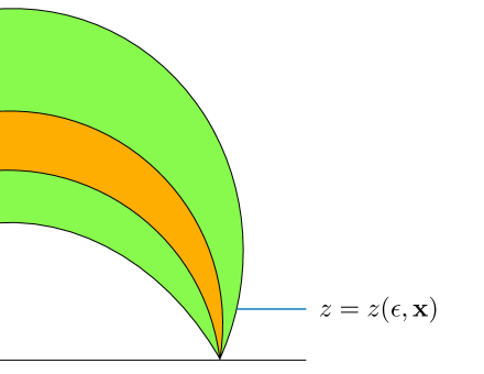
Figure 6: A section of the banana geometry to illustrate the integration surface $\sigma$. The cut-off surface $z=({\bf z},{\bf x}),x=({\bf z},{\bf x})$ can be extended up to the preimage of the wall, the choice of connecting tissues from there to the stretched horizon results in a choice of normalisation.

In the cone, the surface integral on $\vec{c}=(R(\boldsymbol{\epsilon},{\bf R}),z(\boldsymbol{\epsilon},{\bf R}))$ is very explicit, since we know the change of variables (3.6). We find

$${\cal A}_{cone}(\boldsymbol{\epsilon},{\bf R})=\frac{2{\bf R}^{d}}{\boldsymbol{\epsilon}^{d}}-M+\frac{M^{2}}{4^{2}}\frac{\boldsymbol{\epsilon}^{d}}{{\bf R}^{d}}$$ (3.21)

Then, the normal vector $\vec{n}$ is a rotation of $\partial_{{\bf R}}\vec{c}$, and the very definition of the surface integral cancels $|\vec{n}|$, so the measure of the integral becomes

$$\int_{{\bf z}=\boldsymbol{\epsilon}}\!\!d\sigma\,\frac{\vec{u}\cdot\vec{n}}{|\vec{n}|}=\int\frac{d{\bf R}}{\bf R}\left(1-\frac{{\boldsymbol{\epsilon}}^{2}}{{\bf R}^{2}}\frac{1}{k(\frac{\boldsymbol{\epsilon}}{\bf R})}\right)=\int\frac{d{\bf R}}{\bf R}\left(\frac{1}{(1+\frac{\boldsymbol{\epsilon}^{2}}{{\bf R}^{2}})}-\frac{d-1}{d}M\frac{\boldsymbol{\epsilon}^{d+2}}{{\bf R}^{d+2}}+\ldots\right)\,.$$ (3.22)

The whole $k(x)$ is given in eq. (3.6). When taking the $\boldsymbol{\epsilon}\rightarrow 0$ limit, we have to be careful in isolating the AdS contribution in $\vec{u}\cdot\vec{n}$ from the rest because ${\cal A}_{cone}$ itself comes with a Laurent series in $\boldsymbol{\epsilon}$. What we want to ensure is that the corrections to AdS proportional to $M$ do not interfere with the structure of ${\cal A}_{cone}$ as a series in $\boldsymbol{\epsilon}$. This implies that we have to resum the AdS contribution in $\boldsymbol{\epsilon}$ before taking the limit to zero. This is what we made explicit on the right-hand side of eq. (3.22).

The GHY and counterterm contributions at the asymptotic boundary can by definition be evaluated in the FG patch directly. Putting all of these together cancels the usual UV divergence from AdS and a finite result remains,

$$\lim_{\boldsymbol{\epsilon}\rightarrow 0}\frac{1}{16\pi G_{\textrm{\tiny N}}}\int_{{\bf z}=\boldsymbol{\epsilon}}d\sigma\,\frac{\vec{u}\cdot\vec{n}}{|\vec{n}|}{\cal A}(r)+I_{GHY}(\partial_{AdS})+I_{ct}=-\frac{M}{16\pi G_{\textrm{\tiny N}}}\int_{{\bf R}_{\star}}^{1/{\bf R}_{\star}}\frac{d{\bf R}}{\bf R}\,.$$ (3.23)

We can take any ${\bf R}_{\star}\geq\left[\frac{M}{4}\right]^{\frac{1}{d}}\boldsymbol{\epsilon}$, where the limit is the value fixed by the wall. It is worth mentioning that in the cone coordinates, we can compute the onshell action directly by evaluating $\sqrt{\det g_{FG}}$, from ${\bf z}=\boldsymbol{\epsilon}$ to the ${\bf z}=$ wall. Since we know the preimage, i.e., $r_{wall}=M^{\frac{1}{d}}$, we can then check this result against the surface integral done with ${\cal A}$. We find perfect agreement, as it should. In passing, we also notice that ${\cal A}(r_{wall})=0$.

We now repeat the cut-off surface integration for the banana. This time we do not have the full change of variables, however, we can proceed by using the series expansion in ${\bf z}$. The measure factor can be found to generalize the right-hand side of eq. (3.22) into

$$\vec{u}\cdot\vec{n}\big{|}_{{\bf z}=\boldsymbol{\epsilon}}=\frac{{\boldsymbol{\rho}}^{d-2}}{\tilde{\bf R}^{\frac{d}{2}}}\,\frac{{\boldsymbol{\rho}}^{2}+\tilde{\bf x}^{1}(\tilde{\bf x}^{1}-2b\boldsymbol{\epsilon}^{2})}{({\bf R}^{2}+\boldsymbol{\epsilon}^{2})\,\Theta^{2}({\bf x}^{1},{\boldsymbol{\rho}},\boldsymbol{\epsilon})}+MO(\boldsymbol{\epsilon}^{d+1})$$ (3.24)

where ${\bf R}^{2}={\boldsymbol{\rho}}^{2}+({\bf x}^{1})^{2}$, $\tilde{\bf R}^{2}={\boldsymbol{\rho}}^{2}+(\tilde{\bf x}^{1})^{2}$, and $\tilde{\bf x}^{1}={\bf x}^{1}+b\,({\bf R}^{2}+{\bf z}^{2})$. Then ${\cal A}_{banana}=\frac{2\tilde{\bf R}^{d}}{\boldsymbol{\epsilon}^{d}}-M+O(Mb\boldsymbol{\epsilon}^{d},M^{2}\boldsymbol{\epsilon}^{d})$. It follows again that

$$\lim_{\boldsymbol{\epsilon}\rightarrow 0}\frac{1}{16\pi G_{\textrm{\tiny N}}}\int_{{\bf z}=\boldsymbol{\epsilon}}d\sigma\,\frac{\vec{u}\cdot\vec{n}}{|\vec{n}|}{\cal A}(r)+I_{GHY}(\partial_{AdS})+I_{ct}$$ (3.25)

$$\qquad\qquad\qquad\qquad=-\frac{M}{16\pi G_{\textrm{\tiny N}}}\int_{\leavevmode\hbox to14.63pt{\vbox to8.94pt{\text{[drawing]}}}}\frac{{\boldsymbol{\rho}}^{d-2}\,d{\boldsymbol{\rho}}\,d{\bf x}^{1}d\Omega_{d-2}}{(({\bf x}^{1})^{2}+{\boldsymbol{\rho}}^{2})^{d/2}\,((1+b{\bf x}^{1})^{2}+{\boldsymbol{\rho}}^{2})^{{d}/{2}}}\,,$$

where in the remaining integral, we recognise the expression for $f_{2pt}$ familiar from section 2.2, e.g., compare with eq. (2.21).

3.2.2 From cut-off to stretched horizon

At this point, we must consider the two components of the integration surface $\sigma$ comprising connecting tissue extending between the asymptotic cut-off surface and the stretched horizon – see figure 6. The simplest choice is to go straight into the bulk. Other choices are possible, for example, we can use them to match the $z=\epsilon$ surface close to the insertion points. Compared to computations usually done for probe objects, the freedom in cutting the geometry passed the FG wall is something new. To see why consider a geodesic connecting the insertion points. The length of such a geodesic, i.e., $({\bf z}(s),{\bf x}(s))=\ell\,(\sin s,\cos s)$ with $s\in(0,\pi)$, computes the two-point function. The ambient space is just empty AdS and the cut-off is ${\bf z}=\boldsymbol{\epsilon}$, to be understood physically as a UV cut-off or lattice spacing. The range of integration is read off from the equation ${\bf z}(s)=\boldsymbol{\epsilon}$. Equally, we can parametrise the integration with respect to the $\bf{x}$ coordinate. Note at this point, the obvious fact that empty AdS is already in the FG gauge. In particular, there is no extra space which corresponds to integrating over the two connecting tissues between the cut-off and the horizon. It is also clear now that the role of the connecting tissues is simply to change the normalization of the operators, since different tissues yield different normalization constants to the final action.

3.2.3 Stretched horizon

Finally, the stretched horizon contribution is the surface integral on $\vec{c}=(x^{1},\rho,z=z(x^{1},\rho))$, where $z=z(x^{1},\rho)$ solves the equation $r(z,\vec{x})=r_{h}(1+\epsilon^{\prime})$ as we did in (2.19). The normal vector $\vec{n}$ is the cross product $\partial_{x^{1}}\vec{c}\times\partial_{\rho}\vec{c}$, and of course, it becomes proportional to $\partial_{i}r(z,\vec{x})$. Then, similarly to what we did in section 2.2, we look at $z=z_{-}(x^{1},\rho)$, and we extract the logarithmic form close to the insertion points. The relevant integral is

$$I_{hor}=-\frac{1}{16\pi G_{\textrm{\tiny N}}}\int_{A}\frac{\rho^{d-2}d\rho\,dx^{1}\,d\Omega_{d-2}}{\tilde{R}_{-}^{d-1}}\,\frac{b^{2}(1+r_{h}^{2}){\cal A}(r_{h})}{(z_{+}^{2}-z_{-}^{2})(R^{2}+z_{-}^{2})((1+bx^{1})^{2}+b^{2}\rho^{2}+b^{2}z_{-}^{2})}$$ (3.26)

where $\tilde{R}_{-}=\tilde{R}(x^{1},\rho,z=z_{-}(x^{1},\rho))$. Close to the insertion points, the logarithmic form in eq. (3.26) is

$$I_{hor}=-\frac{{\cal A}(r_{h})}{16\pi G_{\textrm{\tiny N}}}\int_{A}\frac{\rho^{d-2}d\rho\,dx^{1}\,d\Omega_{d-2}}{((x^{1})^{2}+\rho^{2})^{d/2}((1+bx^{1})^{2}+b^{2}\rho^{2})^{{d}/{2}}}+{\color[rgb]{1,0,0}\cdots}\,,$$ (3.27)

where again we recognize appearance of $f_{2pt}$. The rest of the terms denoted by the ellipsis are again free of divergences and will only contribute to the normalization.

3.2.4 The onshell action revisited

At this point, we can assemble again the total onshell action,

$$I_{\leavevmode\hbox to14.63pt{\vbox to8.94pt{\text{[drawing]}}}}=I_{bulk}\ +I_{GHY}(\partial_{AdS})+I_{GHY}({\rm stretch})+\ I_{ct}$$ (3.28)

where the contribution in $I_{bulk}$ coming from the asymptotic boundary (i.e., ${\bf z}=\boldsymbol{\epsilon}$) is given in eq. (3.25), and the contribution from the stretched horizon is given in eqs. (3.26) and (3.27). Moreover, we have argued that the boundary components connecting the cut-off surface at the asymptotic boundary and at the stretched horizon only contribute to the overall normalization of the two-point function. To finalize, we need to include the GHY term at the stretched horizon, but this is the same as (2.37). Therefore, by mechanically substituting in all of the contributions, we establish the same result which we found in section 2.2 for the CFT two-point function,

$$I_{\leavevmode\hbox to14.63pt{\vbox to8.94pt{\text{[drawing]}}}}=\Delta\int_{\leavevmode\hbox to14.63pt{\vbox to8.94pt{\text{[drawing]}}}}\!\!d^{d}x\,f_{2pt}\ +{\cal N}.$$ (3.29)

where $\Delta=M$ for the operators, and as we understood the normalization depends on the choice of connecting tissues.

A bonus of our discussion here, compared to that of section 2.2, is that by rewriting the bulk contribution to the onshell action as a manifest surface integral (i.e., the integrand became a total derivative), we could make precise the FG renormalization scheme for the cut-off. Another great advantage of working with a total derivative will be the following observation, or “how to compute the total action without really trying".

Given an ansatz for a gravitational background in global coordinates, we can recast Einstein’s equation as the equation of motion from an effective Lagrangian. With the latter, we look for a conserved (and finite) Noether charge ${\cal Q}(r)$ corresponding to a scaling symmetry [27, 28] in this effective Lagrangian. Since this Noether charge is conserved, it must be a constant satisfying $\partial_{r}{\cal Q}(r)=0$. For the AdS-Schwarzschild in (2.1), this procedure yields

$${\cal Q}(r)=-\tfrac{1}{2}r^{d-1}f^{\prime}(r)+r^{d-2}f(r)-r^{d-2}=-\tfrac{d}{2}M\,.$$ (3.30)

We note that the middle expression above applies for a general ansatz of the form given in eq. (2.1) (i.e., without specifying the specific solution for $f(r)$), while the final constant proportional to $M$ comes from substituting in eq. (2.2).

The utility of the Noether charge is to relate the boundary contributions to the onshell action and the stretched horizon contribution. To see this, we first replace $r^{d-1}f^{\prime}(r)$ term (i.e., the first contribution in the middle expression above) with the GHY term on a surface of constant $r$ in global coordinates, namely

$${\cal G}\equiv 2\sqrt{f(r)}r^{d-2}K=r^{d-1}f^{\prime}(r)+2(d-1)r^{d-2}f(r)\,.$$ (3.31)

where the extrinsic curvature is $K=r^{-d+2}\partial_{r}(r^{d-2}\sqrt{f(r)})$. Similarly, we replace the $r^{d-2}$ term (i.e., the third contribution in the middle expression in eq. (3.30)) using ${\cal A}(r)$ in eq. (3.18). Thus we arrive at the following expression for the Noether charge

$${\cal Q}(r)=-\tfrac{1}{2}{\cal G}(r)+\tfrac{1}{2}{\cal A}(r)+(d-1)r^{d-2}f(r)\,.$$ (3.32)

As our notation indicates, we may evaluate the Noether charge at any radius and so it is interesting to evaluate the above at the horizon $r=r_{h}$. There the last term vanishes since $f(r_{h})=0$, and we are left with the first two. In this form, we don’t have to know the exact gravity solution, but only read off how the constant Noether charge is related to quantities which we need to evaluate at the horizon. In particular, we have the surface term coming from the radial integral in bulk action and the GHY term on the stretched horizon. That is, we may use eq. (3.32) to re-express the surface term in eq. (3.27) along with the GHY term on the stretched horizon in terms of the Noether charge, as desired. Hence combining these contributions with the expression in eq. (3.25), the onshell action becomes

$$I_{\leavevmode\hbox to14.63pt{\vbox to8.94pt{\text{[drawing]}}}} =I_{bulk}\ +I_{GHY}(\partial_{AdS})+I_{GHY}({\rm stretch})+\ I_{ct}$$ (3.33)

$$=\frac{1}{16\pi G_{\textrm{\tiny N}}}\bigg{[}-M-2\lim_{r\rightarrow\infty}{\cal Q}(r)\bigg{]}\int_{\leavevmode\hbox to14.63pt{\vbox to8.94pt{\text{[drawing]}}}}\!\!d^{d}x\,f_{2pt}\ +\ {\cal N}\,.$$ (3.34)

Then the integral can be evaluated as in eq. (2.29), and after restoring the mass normalization $\alpha$ given by eq. (2.3), we recover

$$I_{\leavevmode\hbox to14.63pt{\vbox to8.94pt{\text{[drawing]}}}}=\Delta\,\log\frac{|\vec{x}_{\bullet 1}-\vec{x}_{\bullet 2}|^{2}}{a^{2}}+{\cal N}$$ (3.35)

using $\Delta=M$. Hence we have again demonstrated our claim of deriving the two-point function correlator for huge operators from gravity.

4 Geodesics in the black hole two-point function geometry

As we have been discussing, the insertion of huge operators results in backreaction on the AdS geometry, and we found that our two-point function geometry simply corresponds to a Euclidean black hole presented in a somewhat unusual way. In this section, we study both qualitatively and quantitatively how the motion of geodesics that shoot in from the asymptotic boundary of AdS is affected by the presence on the Euclidean black hole. These geodesics would correspond to the insertion of additional light operators and so this is a first step towards investigating higher point functions with our geometric approach.

Figure 7 illustrates a variety of geodesics originating from points on the asymptotic boundary, with a given velocity. A prominent feature of the plot is that the geodesics shown there do not reach the horizon. In fact, the only geodesics that collide with the horizon are finely tuned. The latter is clearly understood by considering the metric (2.1) in global coordinates. In this setting, it is straightforward to show that the only geodesics reaching $r=r_{h}$ must have a vanishing velocity in the $\tau$ direction. Further, the angular momentum can not be very large (i.e., $|\ell|\leq r_{h}$).

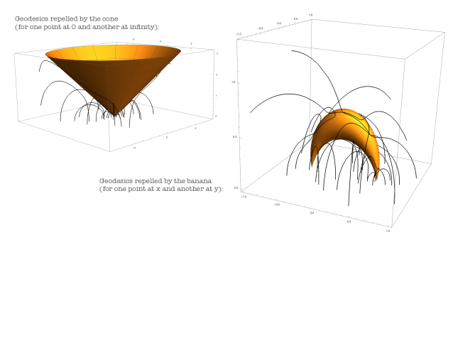
Figure 7: Geodesics moving in the black hole background when the stretched horizon is a cone (left) and when it is a banana (right). Unless finely tuned, geodesics do not collide with the horizon.

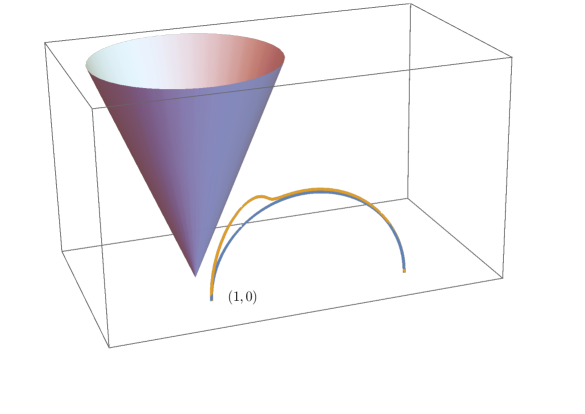
Figure 8: Geodesic slightly deformed by a small black hole cone. The reduced four point function is the difference between the length of the geodesic without the cone (in blue) and the geodesic deformed by the cone (in orange). Here for concreteness we plotted a case where $(x,\bar{x})=(7/6+7i/2,7/6-7i/2)$ and $M=1/5$.

We can also use geodesics to provide probes for a four-point function of two light particles of dimension $m$ in the presence of two maximally heavy operators of dimension $M$, i.e., the black hole banana. This correlator is obtained by evaluating

$$S(M)=m\int\!ds\,\sqrt{g_{\mu\nu}[M]\,\dot{x}^{\mu}(s)\,\dot{x}^{\nu}(s)}$$ (4.1)

where now the geodesic $x^{\mu}(s)$, differently from what we did above, has boundary conditions such that it approaches the two insertions points at the regulated boundary, namely $z=\epsilon$ for $\vec{x}_{\bullet 1}$ and $\vec{x}_{\bullet 2}$. By conformal invariance we can arrange the external points as in figure 8. Thus, the correlator is more precisely given by

$$\langle\phi_{H}(0)\phi_{L}(1)\phi_{L}(x)\phi_{H}(\infty)\rangle=e^{-(S(M)-S(0))}$$ (4.2)

where the right-hand side is finite in $\epsilon$ after subtracting the AdS value.

The computation of $x^{\mu}(s)$ and the action $S$ are described in appendix B. In the $M\to 0$ limit, the result simplifies significantly. For example, in AdS₅/CFT₄ we find

$$S(M)-S(0)=\tfrac{1}{4}mM\times(x-1)(\bar{x}-1)\times\frac{h(x)-h(\bar{x})}{x-\bar{x}}+O(M^{2})\,,$$ (4.3)

where

$$h(x)=\frac{6}{{x}-1}-\frac{\left({x}^{2}+4{x}+1\right)\log\left({x}\right)}{\left({x}-1\right)^{2}}$$ (4.4)

Quite nicely, the right hand side of (4.3) coincides precisely with the t-channel conformal block for dimension $\Delta=4$ and spin $J=2$ in four spacetime dimensions,

$$\log\frac{\langle\phi_{H}(0)\phi_{L}(1)\phi_{L}(x)\phi_{H}(\infty)\rangle}{\langle\phi_{H}(\infty)\phi_{H}(0)\rangle\langle\phi_{L}(x)\phi_{L}(1)\rangle}=\frac{mM}{120}\mathcal{F}(4,2,1-x,1-\bar{x})+O(M^{2})$$ (4.6)

This is the expected result for a graviton exchange dual to the stress-tensor!

In the AdS₃, the action can be computed without expanding at small $M$ and the result reads

$$S(M)-S(0)=-m\log\left((1-M)\frac{z(1-w)^{\frac{1}{2}-\frac{1}{2\sqrt{1-M}}}\bar{z}(1-\bar{w})^{\frac{1}{2}-\frac{1}{2\sqrt{1-M}}}}{w\bar{w}}\right)$$ (4.7)

where $1-w=(1-z)^{\sqrt{1-M}}$. This is nothing but the (logarithm of) the semiclassical heavy-light limit of the Virasoro block, as discussed in [29]. More details are given in appendix B.

Similar conclusions can be obtained in other dimensions. Our computation here fits very well with a more general discussion about Witten diagrams and geodesics given in [30].

5 Discussion

Euclidean correlation functions of very heavy operators have so far been largely unexplored in AdS/CFT. These are dual to full-fledged backreacted geometries with disturbances of the metric running all the way to marked points on the Poincaré boundary of AdS. Each one of such points corresponds to the insertion of a huge operator which spreads out in the bulk and changes the AdS geometry in some way.

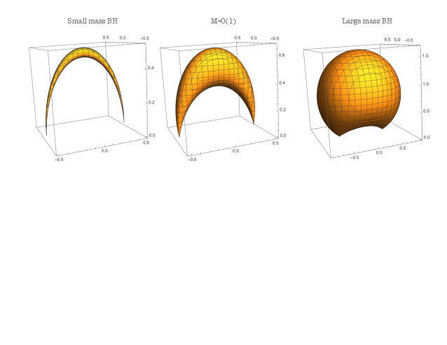
Figure 9: Thin bananas are effectively geodesics. Fat bananas occupy a lot of space.

In this paper, we studied two-point function geometries, and showed that the geometry is nicely understood in terms of a banana foliation, with the tips of the bananas anchored at the insertion points. For smooth geometries, we can shrink the bananas to the geodesic connecting the insertion points. For black holes instead, we can follow the bananas but only up to the location of the stretched horizon. When the black hole is super light, this stretched horizon is approximately occupying the space of a geodesic, on the other hand, when the black hole is very massive it occupies a lot of the AdS space. In all cases, we demonstrated that the onshell action of these two-point black holes reproduces the CFT result for two-point functions (1.1). In particular, the renormalized onshell action has nontrivial spacetime dependence, coming from a logarithmic form at the marked points, and matches the dependence on the dimension $\Delta=M$ as a consequence of a crucial interplay between the boundary contribution at the AdS cut-off, and the boundary term at the stretched horizon.

For holographic two-point functions in AdS, we believe we have unveiled a pretty complete picture. The bananas are special foliation of global AdS, which we obtained from the GtP map, and therefore this map provides a solution generating technique from global AdS geometries to two-point function geometries. It applies to all consistent truncations ansatz in string theory [1], thus AdS bubbles [31, 32], charged clouds [33], and more generally, electric solutions of ${\cal N}=2$ gauged SUGRA with spherically symmetric matter distributions. But there are also gravity solutions which are not consistent truncation ansatz, with interesting topology changes. A well known example are the Lin-Lunin-Maldacena geometries [34] describing all maximally heavy half-BPS operators in $\mathcal{N}=4$ super Yang-Mills. It would be interesting to generalize our results to this case too, especially in the light of the crucial interplay between bulk and boundary contributions that yield in the end the correct two-point function.

Our main motivation for this work, though, was to set up the formalism in general, and apply it to higher point correlation functions. Something preliminary we can say about these is the following. We can always solve the FG form of a given multipoint geometry in a series expansion, once we know the expectation value of the stress-tensor. For example, for three-operators we would find,

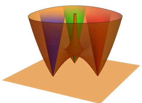
Figure 10: The $\det(g_{\texttt{Banados}})=0$ surface in the three point function case, with $d=2$. The horizons (depicted in RGB), begin as cones. What fate awaits them far beyond the wall?

$$ds^{2}\Big{|}_{FG}=\frac{d{\bf z}^{2}+d\vec{\bf x}^{2}}{{\bf z}^{2}}+\ldots+{\bf z}^{d}\frac{\langle T_{ij}({\bf x})O_{\Delta}({\bf x}_{1})O_{\Delta}({\bf x}_{2})O_{\Delta}({\bf x}_{3})\rangle}{\langle O_{\Delta}({\bf x}_{1})O_{\Delta}({\bf x}_{2})O_{\Delta}({\bf x}_{3})\rangle}+\ldots$$ (5.1)

with the higher order contributions (in ${\bf z}$) determined by Einstein’s equations. However, as we showed in this paper, already for the two points the black hole geometry is a completion of the FG patch, and in particular the horizon lies beyond the wall where $\det g_{FG}=0$. Once again, the information from the stretched horizon was crucial in order to recover the CFT result as function of $\Delta=M$. So, here comes the question. For three- and higher point functions, what lies behind this wall?

Do Euclidean three- and higher point functions of huge operators have anything to do with physics of black holes merging? How sensitive are these geometries to the microscopic details of the operators? How would firewalls or fuzzballs manifest themselves? Do averages play any role in these correlators in lower dimensions? What about in higher dimensions?

This would be a good point to stop, but we cannot resist ourselves from adding two more small comments.

5.1 Comment 1: Three Dimensions

Three dimensions is a great laboratory for developing intuition. In fact, in three dimensions, the exact FG metric was found by Bañados [19] and simply reads

$$ds^{2}=dAdS_{3}+T({\bf x})d{\bf x}^{2}+\bar{T}(\bar{\bf x})d\bar{\bf x}^{2}+{\bf z}^{2}T({\bf x})\bar{T}(\bar{\bf x})d{\bf x}d\bar{\bf x}$$ (5.2)

where $T$ ($\bar{T}$) are the (anti)holomorphic boundary stress tensor. For example, for a scalar three-point function, we have

$$T({\bf x})=-\frac{1}{({\bf x}-x_{1})({\bf x}-x_{2})({\bf x}-x_{3})}\sum_{i\neq j\neq k}\frac{M_{i}x_{ij}x_{ik}}{4({\bf x}-x_{i})}\qquad;\qquad\bar{T}(\bar{\bf x})=T(\bar{\bf x})$$ (5.3)

With this assignment, $ds^{2}$ in eq. (5.2) describes the three-point function geometry for three black holes in AdS₃/CFT₂ of masses $M_{1},M_{2},M_{3}$ inserted at locations $x_{1},x_{2},x_{3}$. As in the two-point function case, this metric has a wall beyond which we need better coordinates to figure out what the geometry does. This wall is much richer than in the two-point function case – see figure 10. What lies behind this wall? What is the full three-point function geometry and what is the corresponding structure constant in the dual field theory? This challenge is the subject of our companion paper [1].

5.2 Comment 2: LLM Three-Point Functions

What about higher dimensions? What about three-point function geometries in ${\cal N}=4$ SYM? – or other maximally symmetric theories in various dimensions?

In global AdS${}_{5}\times$S⁵ the most general half-BPS geometries are LLM geometries [34] (see also [35] for a nice review and for the holographic renormalization aspects of these geometries). In ${\cal N}=4$ SYM, they correspond to operators in the Schur basis [36] of the form

$$\mathcal{O}\propto\chi_{\underline{\lambda}}(y\cdot\phi)$$ (5.4)

with Young diagram $\underline{\lambda}$ of $O(N^{2})$ boxes. The vector $y$ is a six dimensional null vector picking up a particular combination of the six scalars $\phi^{I}$ of the gauge theory. While it would be fascinating to construct general three-point functions of the operators (5.4) from group theory alone, one might start wondering if are there any hints or expectations that would help our intuition? Well, as we discuss below, there are some.

A three-point function,

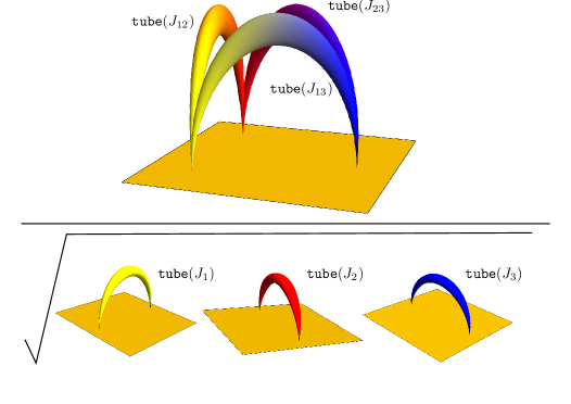
Figure 11: A suggestive explanation for a result like (5.8), where the geometry is foliated by conifolds shooting out of the insertion points like pairwise two-point function geometries.

$$\langle\mathcal{O}_{1}\mathcal{O}_{2}\mathcal{O}_{3}\rangle=\prod_{i<j}\Big{(}\frac{y_{i}\cdot y_{j}}{(x_{i}-x_{j})^{2}}\Big{)}^{J_{ij}}C_{\underline{\lambda}_{1},\underline{\lambda}_{2},\underline{\lambda}_{3}}\,,$$ (5.5)

depends on a fixed kinematical factor, built out of the $J_{ij}$, i.e., the number of propagators between operators $i$ and $j$,

$$J_{12}=\frac{J_{1}+J_{2}-J_{3}}{2}\,,\qquad J_{13}=\frac{J_{1}+J_{3}-J_{2}}{2}\,,\qquad J_{23}=\frac{J_{3}+J_{2}-J_{1}}{2}\,,$$ (5.6)

and by the structure constant $C$, which here is coupling independent, and therefore it can be computed in free $\mathcal{N}=4$ SYM by Wick contractions. Computing $C$ is thus a well-posed but not trivial combinatorial problem for any triplet $\underline{\lambda}_{i=1,2,3}$. It would indeed be great to solve this problem completely, or at least for operators with very large Young diagrams.– In a simple instance, i.e., when the operators are fully symmetric labelled by a Young diagram with a single row of $J$ boxes, we did manage to find the solution (see appendix C for details)

$$\!\!\!\!\tilde{C}^{\texttt{\,symmetric}}_{{J_{1}}{J_{2}}{J_{3}}}\equiv\frac{{}_{3}F_{2}(-J_{12},-J_{13},-J_{23};1,1{-N}-\frac{J_{1}+J_{2}+J_{3}}{2};1)({N})_{\frac{J_{1}+J_{2}+J_{3}}{2}}}{(-)^{\frac{J_{1}+J_{2}+J_{3}}{2}}\sqrt{(-N-J_{1}+1)_{J_{1}}(-N-J_{2}+1)_{J_{2}}(-N-J_{3}+1)_{J_{3}}}}\,.$$ (5.7)

The $\tilde{C}$ is normalised by two-point functions, and the hypergeomtric function $\,{}_{3}F_{2}$ accounts for genuine interactions among the three operators; when the $J_{i=1,2,3}\in\mathbb{N}$ it evaluates to a non trivial polynomial of $N$. In the limit when $J_{i}=N^{2}j_{i}$ the result simplifies to:

$$\log\tilde{C}^{\texttt{symmetric}}_{{J_{1}}{J_{2}}{J_{3}}}\simeq-N^{2}\Big{[}\sum_{ij}\texttt{tube}(j_{ij})-\tfrac{1}{2}\sum_{i}\texttt{tube}(j_{i})\Big{]}\qquad{\rm with}\quad\texttt{tube}(j)=j\log j\,.$$ (5.8)

Even though $\tilde{C}^{\texttt{\,symmetric}}_{{J_{1}}{J_{2}}{J_{3}}}$ is telling us something only about the limit of a regular geometry, where each individual operator is dual to a thin ring that is taken off to infinity with respect to the AdS${}_{5}\times$S⁵ droplet [35], the expression we got is quite suggestive.

In fact, we can rewrite the asymptotics as

$$\lim_{N\gg 1}\underbrace{\frac{J_{1}!J_{2}!J_{3}!}{(\frac{J_{1}+J_{2}-J_{3}}{2})!(\frac{J_{1}+J_{3}-J_{2}}{2})!(\frac{J_{2}+J_{3}-J_{1}}{2})!}\times\frac{1}{\sqrt{J_{1}!J_{2}!J_{3}!}}}_{\ \ \ \ \#{\tt\,Wick\ contractions\ at\ 3pt}\ \ \ \times\ \ \ {\tt 2pt\ normalisation}}\ \simeq\ e^{N^{2}\left[\frac{1}{2}\sum_{i}j_{i}\log j_{i}-\sum_{ij}j_{ij}\log j_{ij})\right]}$$ (5.9)

showing that it coincides with the leading asymptotics of the number of Wick contractions for three-points, when $J_{i}=N^{2}j_{i}$, divided by two-point normalizations. In other words, we get the a purely combinatorial result. Note now that a LLM geometry generically involves multi-particle states and that the ${\tt tube}$ function is the building block for the two-point function normalization. So what if when $J\gg N$ the operator ${\cal O}$ breaks apart and the bulk geometry is foliated as in figure 11? with conifold geometries emerging from the insertion points?

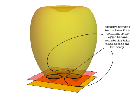
Figure 12: Another scenario where operators in the bulk merge, but the dominant contribution to the action is effectively pairwise because the geometry change is huge.

Another scenario, which was inspired to us by a beautiful talk of David Simmons-Duffin at KITP this January, is represented in figure 12 – see [38]. There we imagine that each operator shoots from the boundary a huge geometry change, like the fat bananas in the figure, so that interactions among the three operators are effectively pairwise. This scenario could also reproduce something like eq. (5.8).

We look forward to continuing to explore huge correlators, from the boundary, as well as from the bulk.

Appendix A Euclidean Rotation

In this section we describe the GtP map with marked points $0$ and $\infty$ as a certain rotation in embedding coordinates. This rotation is precisely the one used in [2] to map spinning strings in global AdS to Euclidean strings in Poincaré AdS with two-point function boundary conditions. Here we will promote it to a local change of coordinates.

In embedding coordinates, AdS admits the following standard parametrisations

$$\begin{array}[]{l}\rule{14.22636pt}{0.0pt}{\tt global\ Lorentzian}\rule{56.9055pt}{0.0pt}{\tt Euclidean\ Poincare}\\[5.69046pt] \hline\cr\begin{array}[]{rl c|c cl}&&&&&\\ X_{i}&=r\ \Omega_{i}\,,\ \ i\geq 1&&&X_{i+1}&=x^{i}/\tilde{z}\,,\ \ {i\geq 1}\\[2.84544pt] &\,\vdots&&&\ \ X_{1}&=\frac{1}{2\tilde{z}}(1-R^{2}-\tilde{z}^{2})\\[2.84544pt] X_{0}&=\sqrt{1+r^{2}}\,\sin t&&&\ \ X_{0}&=x^{0}/\tilde{z}\\[2.84544pt] X_{-1}&=\sqrt{1+r^{2}}\,\cos t&&&\ \ X_{-1}&=\frac{1}{2\tilde{z}}(1+R^{2}+\tilde{z}^{2})\end{array}\end{array}$$ (A.1)

where $\Omega_{i}$ are spherical coordinates, and $R^{2}=\sum_{i=0}^{d-1}(x^{i})^{2}$. Black holes will live in $D=d+1$ dimensions, with $d$ being the spacetime dimension of the AdS boundary.

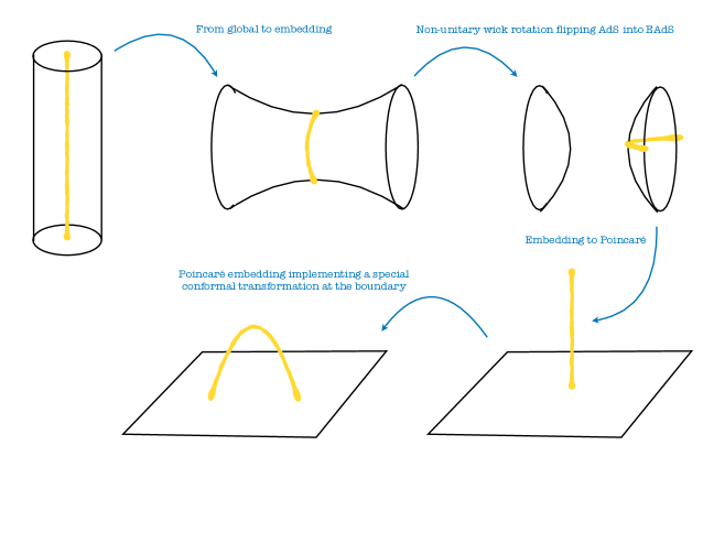
Figure 13: Schematic for the sequence of transformations from global AdS with Lorentzian signature to the euclidean Poincaré patch. Starting with a tubular object in the middle of AdS, we end up with a banana shape with two insertion points at the boundary of AdS. The direct transformation from the top left to the bottom right pictures is eq. (2.5).

Recall the Schwarzschild black hole solution in global with Lorentzian signature is,

$${\tt global}\quad;\quad ds_{D}^{2}=\frac{dr^{2}}{g_{\tau\tau}(r)}-g_{\tau\tau}(r)dt^{2}+r^{2}d\Omega^{2}_{D-2}$$ (A.2)

We will change signature by considering $\tau=-it$. Our starting point is then the following relations

$$\begin{array}[]{l}dt=\frac{X_{-1}\,dX_{0}-X_{0}\,dX_{-1}}{1+r^{2}}\\[8.5359pt] dr=\frac{X_{0}\,dX_{0}+X_{-1}\,dX_{-1}}{r}\\[8.5359pt] d\Omega_{D-2}^{2}=-\frac{dr^{2}}{r^{2}}+\tfrac{1}{r^{2}}\sum_{i\geq 1}dX^{2}_{i}\end{array}\qquad;\qquad r=\sqrt{X_{-1}^{2}+X_{0}^{2}-1}$$ (A.3)

which we can use to rewrite eq. (A.2). Then, the rotation of [2] into Euclidean AdS is $X_{0}\rightarrow iX_{1}$ and $X_{1}\rightarrow X_{0}$. Once we perform this rotation on eq. (A.3), we will rewrite the result by the using Euclidean Poincaré patch, i.e., the second column of table (A.1). This gives the change of coordinates in the differential form,

$$\begin{array}[]{rl}\left[\begin{array}[]{c}d\tau\\[5.69046pt] dr\end{array}\right]=&\frac{1}{\tilde{z}}\left[\begin{array}[]{cc}\frac{R\,\tilde{z}}{\tilde{z}^{2}+R^{2}}&\frac{\tilde{z}^{2}}{\tilde{z}^{2}+R^{2}}\\[5.69046pt] 1&-\frac{R}{\tilde{z}}\end{array}\right]\left[\begin{array}[]{c}dR\\[5.69046pt] d\tilde{z}\end{array}\right]\end{array}$$ (A.4)

where $R,\Omega_{i}$ are polar coordinates in Poincaré AdS. As it turns our the $d\Omega$ are invariant, since in fact we are preserving rotational symmetry. Upon integration, we find

$$\tau=\frac{1}{2}\log(\tilde{z}^{2}+R^{2})\qquad{\rm and}\qquad r=\frac{R}{\tilde{z}}\,,$$ (A.5)

which is precisely the AdS-unitary transformation in eq. (2.5).

Appendix B Geodesics in the banana background

In this appendix, we show how to solve the problem of a geodesic the background of a two-point function black hole, and for concreteness we will specialize to AdS₅ and AdS₃. Other odd bulk dimensions (i.e., even boundary dimensions) can be analyzed with the same tools that we provide, but expressions become more complicated. We are working with the cone metric eq. (2.6).

B.1 AdS₅ geodesics

We can always put the four external points on a two-dimensional plane, through a conformal transformation, therefore the geodesic can be restricted to explore a three-dimensional space, the plane plus the holographic direction. We have $\tilde{z}(s)$, $R(s)$ and $\phi(s)$ or equivalently $\eta\equiv\tilde{z}/R$, $\rho\equiv\log(R)$ and $\phi$. The latter will simplify the problem since they are essentially the same as in global coordinates (2.1).

Now, the cone geometry (2.6) is invariant under dilatations $(R,\tilde{z})\to\lambda(R,\tilde{z})$ and $SO(d-1)$ rotations. For the three-dimensional problem, we have two conserved charges for geodesics which we denote as $\mathcal{E}$ and $\mathcal{J}$. By using these charges, we obtain first order equations

$$\!\!\!\!\!\!\!\!\!\!\!\!\!\!\!\!\!\!\phi^{\prime}={\pm}\frac{\mathcal{J}\eta\eta^{\prime}}{\sqrt{\mathcal{J}^{2}M\eta^{6}-\left(\mathcal{J}^{2}+M\right)\eta^{4}-\eta^{2}\left(\mathcal{J}^{2}+\mathcal{E}^{2}-1\right)+1}}$$ (B.1)

$$\!\!\!\!\!\!\!\!\!\!\!\!\!\!\!\!\!\!\rho^{\prime}=\pm\frac{\mathcal{E}\eta\eta^{\prime}}{\left(1+\eta^{2}-M\eta^{4}\right)\sqrt{\mathcal{J}^{2}M\eta^{6}-\left(\mathcal{J}^{2}+M\right)\eta^{4}-\eta^{2}\left(\mathcal{J}^{2}+\mathcal{E}^{2}-1\right)+1}}-\frac{\eta\eta^{\prime}}{\eta^{2}+1}$$ (B.2)

In total the solution is parametrized by four integration constants, ${\cal E},{\cal J}$ and $C_{\rho},C_{\phi}$ from these first order equations.

It is straightforward to solve eq. (B.2) for empty AdS with ${\cal J}=0$. This gives the semicircle in the form,

$$\big{[}R(\eta)-R_{0}\big{]}^{2}+\big{[}\tilde{z}=\eta R(\eta)\big{]}^{2}=L^{2}\qquad;\qquad\begin{array}[]{c}R=\frac{C}{{\cal E}\pm\sqrt{1-({\cal E}^{2}-1)\eta^{2}}}\\[14.22636pt] {\cal E}=\frac{R_{0}}{L}\quad;\quad C=\frac{R_{0}^{2}-L^{2}}{L}\end{array}$$ (B.3)

The signs $\pm$ provide a parametrization for the two branches of the semicircle, each one going from one insertion point at $z=0\rightarrow\eta=0$ up to the turning point $\eta_{\star}$, where the derivatives blow up. This is given by the solution of $1-({\cal E}^{2}-1)\eta_{\star}^{2}=0$. Note that since $\eta\geq 0$, in our conventions ${\cal E}\geq 1$. The limit where the insertion points are close to each other is the limit ${\cal E}\rightarrow\infty$, since $\eta_{\star}$ and thus $\tilde{z}_{\star}$ goes to zero. Note also the connection with global coordinates, since we can rewrite

$$\rho^{\prime}+\frac{\eta\eta^{\prime}}{\eta^{2}+1}=\frac{d}{ds}\frac{\log\big{(}z(s)^{2}+R(s)^{2}\big{)}}{2}=\tau^{\prime}(s)$$ (B.4)

Of course, $\phi$ in the cone is the same as in global coordinates.

In the black hole case, the polynomial in the square root is a cubic in $\eta^{2}$ and has three zeros. One (and only one of them) of them is finite for $M\to 0$ and ${\cal J}\to 0$. This one defines the turning point $\eta_{*}>0$. By construction this turning point has a good limit to empty AdS.

Figure 14: We plot the right hand side of eq. (B.6) on the line $x=\bar{x}\geq 1$. The result can be written through elementary functions, and it reads
$\log(x)=H_{+}+H_{-}\quad;\quad H_{\pm}=\mp\frac{\cal E}{\sqrt{1+4M}}\frac{1}{\sqrt{1-\left(\mathcal{E}^{2}-1\right)\eta^{2}_{\mp}-M\eta_{\mp}^{4}}}\times\left(\coth^{-1}\left[\frac{\sqrt{1-\left(\mathcal{E}^{2}-1\right)\eta_{\mp}^{2}-M\eta_{\mp}^{4}}}{2-({\cal E}^{2}-1)\eta_{\mp}^{2}}\right]\pm\frac{i}{2}\right)$
with $\eta^{2}_{\pm}=(1\pm\sqrt{1+4M})/(2M)$. For empty AdS, $\log(x)$ blows up at ${\cal E}=1$, which implies that there is a geodesic for any two insertion points, with no limits on their separation. For the black hole, $M>0$, the range of $\log(x)$ is bounded, thus real geodesics connect insertion points only up to some distance.

Eqs. (B.1) and (B.2) can be integrated to obtain the shifts. For the right-hand side, we sum the integrals from $0\leq\eta\leq\eta_{\star}$ for the first branch and the $\eta_{\star}\leq\eta\leq 0$ for the second branch. For the left-hand side, we then consider the external points as described in figure 8. In sum we find

$$\!\!\!\!\!\!\!\underbrace{-i\log\sqrt{{x}/{\bar{x}}}}_{\Delta\phi} =2\int\limits_{0}^{\eta_{*}}\!\!d\eta\frac{\mathcal{J}\eta}{\sqrt{\mathcal{J}^{2}M\eta^{6}-\left(\mathcal{J}^{2}+M\right)\eta^{4}-\eta^{2}\left(\mathcal{J}^{2}+\mathcal{E}^{2}-1\right)+1}}$$ (B.5)

$$\!\!\!\!\!\!\!\underbrace{\log\sqrt{x\bar{x}}}_{\Delta\rho} =2\int\limits_{0}^{\eta_{*}}\!\!d\eta\frac{\mathcal{E}\eta}{\left(1+\eta^{2}-M\eta^{4}\right)\sqrt{\mathcal{J}^{2}M\eta^{6}-\left(\mathcal{J}^{2}+M\right)\eta^{4}-\eta^{2}\left(\mathcal{J}^{2}+\mathcal{E}^{2}-1\right)+1}}$$ (B.6)

These integrals express the physical insertion points $x,\bar{x}$ in terms of ${\cal E}$ and ${\cal J}$. They can be computed but the result is written terms of elliptic functions so not very illuminating, and so we omit it.

A somewhat subtle point in the computation is that for some $x,\bar{x}$, a real solution to these equations will not exist, see figure 14. Implicitly, we invert the relation (B.6) in a finite domain where this inverse exists (with a real solution) and analytically continue from there to access the result for any $x,\bar{x}$.

To obtain the action we can directly substitute eqs. (B.1) and (B.2) into the action to find

$$S(M)=m\left(\int_{\epsilon}^{\eta_{*}}+\int_{\frac{\epsilon}{\sqrt{x\bar{x}}}}^{\eta_{*}}\right)\frac{d\eta}{\eta}\frac{1}{\sqrt{\mathcal{J}^{2}M\eta^{6}-\eta^{4}\left(\mathcal{J}^{2}+M\right)-\eta^{2}\left(\mathcal{J}^{2}+\mathcal{E}^{2}-1\right)+1}}$$ (B.7)

Note that when computing $S(M)-S(0)$ the $\epsilon$ divergent terms coming from the lower integration limit drop out nicely and we can simply take $\epsilon\to 0$ there. This combination is what gives us the relevant four point function with stripped off two-point function prefactors.

We will now make progress analytically in the result by taking some limits.

B.1.1 Small black holes $M\to 0$

If we expand the equations above at small $M$ all integrals become trivial to compute in terms of functions like log and arctan. We then easily find

$$\!\!\!\!\!\!\!\!\!\!\!\!\!\!\!\!\!\!\!\!S(M)-S(0)=M{\color[rgb]{0,0,1}\left(-\frac{\left(z^{2}+4z+1\right)\left(\bar{z}-1\right)\log(z)}{4(z-1)\left(z-\bar{z}\right)}+\frac{(z-1)\left(\bar{z}^{2}+4\bar{z}+1\right)\log\left(\bar{z}\right)}{4\left(z-\bar{z}\right)\left(\bar{z}-1\right)}-\frac{3}{2}\right)}$$ (B.8)

$$\!\!\!\!\!\!\!\!\!\!\!\!\!\!\!\!\!\!\!\!+M^{2}{\color[rgb]{1,0,1}\Big{(}\tfrac{8z^{2}\bar{z}^{2}+z^{2}\bar{z}+z\bar{z}^{2}-106z\bar{z}+43\bar{z}^{2}+\bar{z}+43z^{2}+z+8}{16\left(z-\bar{z}\right)^{2}}}$$

$${\color[rgb]{1,0,1}\!\!\!\!\!\!\!\!\!\!\!\!\!\!\!\!\!\!\!\!-\tfrac{(z-1)\left(z^{2}\bar{z}^{4}-2z^{2}\bar{z}^{3}+6z^{2}\bar{z}^{2}+24z^{2}\bar{z}+5\bar{z}^{4}-10z\bar{z}^{3}+24\bar{z}^{3}-48z\bar{z}^{2}+6\bar{z}^{2}-10z\bar{z}-2\bar{z}+5z^{2}+1\right)\log\bar{z}}{16\left(z-\bar{z}\right)^{3}\left(\bar{z}-1\right)}}$$

$${\color[rgb]{1,0,1}\!\!\!\!\!\!\!\!\!\!\!\!\!\!\!\!\!\!\!\!+\tfrac{\left(\bar{z}-1\right)\left(z^{4}\bar{z}^{2}-2z^{3}\bar{z}^{2}-10z^{3}\bar{z}+6z^{2}\bar{z}^{2}-48z^{2}\bar{z}+24z\bar{z}^{2}-10z\bar{z}+5\bar{z}^{2}+5z^{4}+24z^{3}+6z^{2}-2z+1\right)\log z}{16(z-1)\left(z-\bar{z}\right)^{3}}}$$

$${\color[rgb]{1,0,1}\!\!\!\!\!\!\!\!\!\!\!\!\!\!\!\!\!\!\!\!+\tfrac{\left(z^{4}\bar{z}^{3}-2z^{4}\bar{z}^{2}-5z^{4}\bar{z}+z^{3}\bar{z}^{4}+16z^{3}\bar{z}^{3}+8z^{3}\bar{z}^{2}-32z^{3}\bar{z}-2z^{2}\bar{z}^{4}+8z^{2}\bar{z}^{3}+24z^{2}\bar{z}^{2}+8z^{2}\bar{z}-5z\bar{z}^{4}-32z\bar{z}^{3}+8z\bar{z}^{2}+16z\bar{z}-5\bar{z}^{3}-2\bar{z}^{2}+\bar{z}-5z^{3}-2z^{2}+z\right)\log z\log\bar{z}}{16\left(z-\bar{z}\right)^{4}}}$$

$${\color[rgb]{1,0,1}\!\!\!\!\!\!\!\!\!\!\!\!\!\!\!\!\!\!\!\!-\tfrac{\left(\bar{z}-1\right)^{2}\left(z^{6}\bar{z}+z^{5}\bar{z}^{2}+16z^{5}\bar{z}-4z^{4}\bar{z}^{2}-13z^{4}\bar{z}-6z^{3}\bar{z}^{2}-80z^{3}\bar{z}+20z^{2}\bar{z}^{2}-13z^{2}\bar{z}+25z\bar{z}^{2}+16z\bar{z}+\bar{z}+25z^{5}+20z^{4}-6z^{3}-4z^{2}+z\right)\log^{2}z}{32(z-1)^{2}\left(z-\bar{z}\right)^{4}}}$$

$${\color[rgb]{1,0,1}\!\!\!\!\!\!\!\!\!\!\!\!\!\!\!\!\!\!\!\!-\tfrac{(z-1)^{2}\left(z^{2}\bar{z}^{5}-4z^{2}\bar{z}^{4}-6z^{2}\bar{z}^{3}+20z^{2}\bar{z}^{2}+25z^{2}\bar{z}+z\bar{z}^{6}+16z\bar{z}^{5}+25\bar{z}^{5}-13z\bar{z}^{4}+20\bar{z}^{4}-80z\bar{z}^{3}-6\bar{z}^{3}-13z\bar{z}^{2}-4\bar{z}^{2}+16z\bar{z}+\bar{z}+z\right)\log^{2}\bar{z}}{32\left(z-\bar{z}\right)^{4}\left(\bar{z}-1\right)^{2}}\Big{)}}+O(M^{3})$$

The first line is just the conformal block for the graviton exchange as we saw in the main text. The second line should correspond to an exchange of two gravitons. Indeed we find an infinite sum precisely compatible with that interpretation (it is infinite since the two massless gravitons can easily form states of any spin and twist)

blue $$= c^{(1)}_{4,2}\times\mathcal{F}_{4,2}(w,\bar{w})\qquad,\qquad(w,\bar{w})=(1-z,1-\bar{z})$$ (B.9)

magenta $$= \sum_{J=0}^{\infty}\sum_{\Delta=\text{max}(8,4+J)}^{\infty}c^{(2)}_{\Delta,J}\mathcal{F}_{\Delta,J}(w,\bar{w})$$ (B.10)

where $c^{(1)}=-1/120$. We could find several trajectories for $c^{(2)}$ but not a closed expression. For example

$$c^{(2)}_{4+J,J}=-\frac{\sqrt{\pi}2^{-2J-5}(J-2)J\left(J^{4}+6J^{3}+35J^{2}+78J-72\right)\Gamma(J-3)}{(J+2)(J+4)(J+6)\Gamma\left(J+\frac{3}{2}\right)}\,,\qquad J=4,6,8,\dots$$

$$c^{(2)}_{\Delta,0}=-\frac{\pi 4^{-\Delta-4}\left(32\Delta^{6}-429\Delta^{5}+1410\Delta^{4}+1660\Delta^{3}-10472\Delta^{2}+2144\Delta+7680\right)\Gamma\left(\frac{\Delta}{2}-1\right)^{2}}{5(\Delta-5)\Gamma\left(\frac{\Delta-1}{2}\right)\Gamma\left(\frac{\Delta+3}{2}\right)}\,,$$

$$\qquad\qquad\qquad\qquad\qquad\qquad\qquad\qquad\qquad\qquad\qquad\qquad\qquad\qquad\qquad\qquad\Delta=8,10,12,\dots$$

And so on.

It would be interesting to see what changes in higher curvature gravity. In particular, it would be interesting if some structure constants would become negative for swampland values of these curvature coefficients.

B.1.2 Radial Geodesics and OPE

Another regime where we get remarkable simplifications is when we put the four points on a line. Then $x=\bar{x}$, and therefore ${\cal J}=0$. All formulae in section (B.1) simplifies and for example the action simply reads

$$S(M)-S(0)=-\frac{m}{2}\log(1+4M-2\mathcal{E}^{2}+\mathcal{E}^{4})-(M\to 0)$$ (B.11)

which is thus parametrically a function of $x$. It is nice to consider the OPE expansion for $x\to 1$ so that the geodesic stays close to the boundary. This limit is the limit of large energy ${\cal E}\gg 1$, and we can expand all expressions in that limit trivially to any desired OPE order and for any mass $M$. Using $w=1-x$ we find

$$S(M)-S(0) = {\color[rgb]{0,0,1}-\frac{M}{40}}w^{4}{\color[rgb]{0,0,1}-\frac{M}{20}}w^{5}{\color[rgb]{0,0,1}-\frac{M}{14}}w^{6}{\color[rgb]{0,0,1}-\frac{5M}{56}}w^{7}+\left({\color[rgb]{0,0,1}-\frac{5M}{48}}{\color[rgb]{1,0,1}-\frac{11M^{2}}{14400}}\right)w^{8}$$

$$+ \left({\color[rgb]{0,0,1}-\frac{7M}{60}}{\color[rgb]{1,0,1}-\frac{11M^{2}}{3600}}\right)w^{9}+\left({\color[rgb]{0,0,1}-\frac{7M}{55}}{\color[rgb]{1,0,1}-\frac{37M^{2}}{4928}}\right)w^{10}+\left({\color[rgb]{0,0,1}-\frac{3M}{22}}{\color[rgb]{1,0,1}-\frac{1081M^{2}}{73920}}\right)w^{11}$$

$$+ \left({\color[rgb]{0,0,1}-\frac{15M}{104}}{\color[rgb]{1,0,1}-\frac{1011M^{2}}{40768}}w-\frac{89M^{3}}{1872000}\right)w^{12}+\left({\color[rgb]{0,0,1}-\frac{55M}{364}}{\color[rgb]{1,0,1}-\frac{39083M^{2}}{1019200}}-\frac{89M^{3}}{312000}\right)w^{13}$$

$$+ \left({\color[rgb]{0,0,1}-\frac{11M}{70}}{\color[rgb]{1,0,1}-\frac{82079M^{2}}{1478400}}-\frac{21991M^{3}}{22176000}\right)w^{14}+\left({\color[rgb]{0,0,1}-\frac{13M}{80}}{\color[rgb]{1,0,1}-\frac{4525M^{2}}{59136}}-\frac{1657M^{3}}{633600}\right)w^{15}$$

$$+ O(w^{16})$$

Note that although this is not a small $M$ expansion, it is automatically organized as one as expected physically. Namely, the more subleading the OPE is, the more primary gravitons are being exchanged and thus more powers of $M$ appear. The linear and quadractic terms in $M$ agree with general limit of the previous section when taken the line.

B.2 AdS₃ geodesics

In this case the problem is simpler, since the blackening factor $f(r)=r^{2}+1-M$ is polynomial. We will introduce the quantity $r_{h}^{2}=M-1$. Note that there are two regimes: the black hole regime where $M>1$ and $r_{h}\geq 0$ is real, the defect regime where $0\leq M\leq 1$ and $r_{h}$ is imaginary. We will be careful in the following in finding expressions for the geodesic where the transitions is smooth.

The AdS₃ equations of motions are

$$\phi^{\prime} ={\pm}\frac{\mathcal{J}\eta\eta^{\prime}}{\sqrt{r_{h}^{2}\mathcal{J}^{2}\eta^{4}-(\mathcal{E}^{2}+\mathcal{J}^{2}+r_{h}^{2})\eta^{2}+1}}$$ (B.13)

$$r^{\prime} =\pm\frac{\mathcal{E}\eta\eta^{\prime}}{\left(1-r_{h}^{2}\eta^{2}\right)\sqrt{r_{h}^{2}\mathcal{J}^{2}\eta^{4}-(\mathcal{E}^{2}+\mathcal{J}^{2}+r_{h}^{2})\eta^{2}+1}}-\frac{\eta\eta^{\prime}}{\eta^{2}+1}$$ (B.14)

The square root contains only a quadratic expression in $\eta^{2}$, so there are only two roots.

$$\eta^{2}_{\pm}=\frac{{\cal J}^{2}+r_{h}^{2}+{\cal E}^{2}\pm\sqrt{({\cal J}^{2}+r_{h}^{2}+{\cal E}^{2})^{2}-4{\cal J}^{2}r_{h}^{2}}}{2{\cal J}^{2}r_{h}^{2}}$$ (B.15)

The turning point corresponds to $\eta_{\star}=\eta_{-}$, since this is the one that can go to the boundary $\eta=0=z$. As in AdS₅ – see eqs. (B.5) and (B.6) – we can integrate these expressions to find the shifts in $\phi$ and $r$. One might notice that the square root in $\eta_{\pm}$ is simply,

$$({\cal J}^{2}+r_{h}^{2}+{\cal E}^{2})^{2}-4{\cal J}^{2}r_{h}^{2}\ \ =\prod_{\begin{subarray}{c}s_{1}=\pm\\ s_{2}=\pm\end{subarray}}({\cal J}+s_{1}r_{h}+is_{2}{\cal E})$$ (B.16)

Then, the combinations that appear after doing the integrals are such that the result can be written as

$$\underbrace{-i\log\sqrt{{x}/{\bar{x}}}}_{\Delta\phi}=\frac{\log\frac{({\cal J}+r_{h}+i{\cal E})({\cal J}+r_{h}-i{\cal E})}{({\cal J}-r_{h}-i{\cal E})({\cal J}-r_{h}+i{\cal E})}}{2r_{h}}\qquad;\qquad\underbrace{\log\sqrt{x\bar{x}}}_{\Delta\rho}=\frac{\log\frac{({\cal J}-r_{h}+i{\cal E})({\cal J}+r_{h}-i{\cal E})}{({\cal J}-r_{h}-i{\cal E})({\cal J}+r_{h}+i{\cal E})}}{2ir_{h}}$$ (B.17)

These function have a smooth transition from the defect to the black hole regime. It is also interesting to see how both remain real. In the defect regime, $r_{h}$ is imaginary. By checking the argument of the log on the r.h.s. of $\Delta\phi$, this is a phase, and so $\Delta\phi$ is real, similarly, by checking the argument of the log on the r.h.s. of $\Delta\rho$, this is a radius, so $\Delta\rho$ is again real. In the black hole regime $r_{h}$ is real, and the opposite happens.

We can now compute the action for the geodesic, by substituting $\phi^{\prime}$ and $r^{\prime}$,

$$S(M) =m\left(\int_{\frac{\epsilon}{1}}^{\eta_{*}}+\int_{\frac{\epsilon}{\sqrt{z\bar{z}}}}^{\eta_{*}}\right)\frac{d\eta}{\eta}\frac{1}{\sqrt{(M-1)\mathcal{J}^{2}\eta^{4}-(\mathcal{E}^{2}+\mathcal{J}^{2}+M-1)\eta^{2}+1}}$$ (B.18)

This integral receives no contribution from $\eta_{\star}$, and it is log divergent,

$$S(M) =-\frac{m}{2}\log\Bigg{[}\frac{\epsilon^{4}}{16x\bar{x}}\prod_{s_{1}=\pm,s_{2}=\pm}({\cal J}+s_{1}r_{h}+is_{2}{\cal E})\Bigg{]}$$ (B.19)

The next step is to invert ${\cal E},{\cal J}$ in terms of $\Delta\rho,\Delta\phi$, thus $x,\bar{x}$. For real values of ${\cal E},{\cal J}$ the range of $x,\bar{x}$ is restricted on a certain domain, which is less than the whole boundary of AdS. With this understanding we find,

$$S(M) =-\frac{m}{2}\log\Bigg{[}\frac{\epsilon^{4}r_{h}^{4}}{4x\bar{x}}\frac{1}{(\cosh(ir_{h}\Delta\rho)-\cosh(r_{h}\Delta\phi))^{2}}\Bigg{]}$$ (B.20)

$$=-\frac{m}{2}\log\Bigg{[}\frac{\epsilon^{4}r_{h}^{4}x^{-ir_{h}-1}\bar{x}^{-ir_{h}-1}}{(1-x^{-ir_{h}})^{2}(1-\bar{x}^{-ir_{h}})^{2}}\Bigg{]}$$ (B.21)

For $r_{h}=i$, i.e., empty AdS, the result becomes $S(0)=-\frac{m}{2}\log[\frac{\epsilon^{4}}{(1-x)^{2}(1-\bar{x})^{2}}]$. The geodesic 4pt correlator in the BTZ background is

$$\!\!\!\!\!\frac{\langle\phi_{H}(0)\phi_{L}(1)\phi_{L}(x)\phi_{H}(\infty)\rangle}{\langle\phi_{H}(\infty)\phi_{H}(0)\rangle\langle\phi_{L}(x)\phi_{L}(1)\rangle} =e^{-(S(M)-S(0))}=$$

$$=\left[(1-M)\frac{(1-x)x^{\frac{\sqrt{1-M}-1}{2}}(1-\bar{x})\bar{x}^{\frac{\sqrt{1-M}-1}{2}}}{(x^{\sqrt{1-M}}-1)(\bar{x}^{\sqrt{1-M}}-1)}\right]^{m}$$ (B.22)

Note this is invariant under $x\rightarrow 1/x$ and $\bar{x}\rightarrow 1/\bar{x}$, as it should. Quite nicely, the result is simply the Virasoro block in the t-channel orientation. In the defect regime, we can expand at small $M$ to get,

$$\!\!\!\!\!\frac{\langle\phi_{H}(0)\phi_{L}(1)\phi_{L}(x)\phi_{H}(\infty)\rangle}{\langle\phi_{H}(\infty)\phi_{H}(0)\rangle\langle\phi_{L}(x)\phi_{L}(1)\rangle}=1+\frac{mM}{24}\left((1-x)^{2}{}_{2}F_{1}(2,2,4;1-x)+c.c.\right)+O(M^{2})$$ (B.23)

which at leading order is just the stress tensor global conformal block.

Appendix C Schur 3-pt functions: a new exact and non-extremal result

In this appendix we will derive a new exact formula for three-point function of half-BPS operators given by fully symmetric (or anti-symmetric) characters. As will any three-point function of half-BPS correlators, this correlation function can be computed at tree level, by working out the combinatoric of Wick contractions.

There are plenty of exact three-point correlators of half-BPS operators computed in this way in the the literature but most of them – if not all – were computed for extremal correlators where the length of one operator is equal to the sum of the other two and thus there are no propagators between those two smaller operators. The main novelty of this appendix is that we will consider a maximally non-extremal correlator where all fields are connected to all fields.

The starting point reads

$$\left\langle\prod_{i=1}^{3}\text{det}[1+t_{i}\,Y_{i}\cdot\Phi_{i}(x_{i})]^{\pm 1}\right\rangle=$$ (C.1)

$$\qquad=C\int\prod_{i\neq j}d\rho_{ij}e^{\,\frac{2N}{g^{2}}\sum\limits_{i<j}\rho_{ij}\rho_{ji}}(1-\hat{\rho}_{12}\hat{\rho}_{12}-\hat{\rho}_{13}\hat{\rho}_{31}-\hat{\rho}_{23}\hat{\rho}_{32}+\hat{\rho}_{12}\hat{\rho}_{23}\hat{\rho}_{31}+\hat{\rho}_{13}\hat{\rho}_{32}\hat{\rho}_{21})^{\pm N}$$

This formula is derived following [39, 40]: One (1) introduces a set of auxiliary fields $\chi$ to cast the determinants as Gaussian integrals; (2) integrates out the scalars $\Phi$ to obtain a quartic action in the auxiliary field; (3) introduce a second set of auxiliary fields $\rho$ to render that quartic interation quadractic using the usual Hubbard-Stratonovich trick; (4) integrate out the now quadractic fields $\chi$ to arrive at (C.1).

The dependence on the generating function variables $t_{j}$ and on the positions and polarizations on the right hand side of (C.1) is hidden inside the hatted variables

$$\hat{\rho}_{ij}\equiv\rho_{ij}\times\sqrt{4t_{i}t_{j}\frac{Y_{i}\cdot Y_{j}}{x_{ij}^{2}}}\,.$$ (C.2)

Each determinant is a generating function of characters of fully anti-symmetric ($+$ sign) or symmetric ($-$ sign) characters so to get the correlation function of the desired characters we simply need to pick up the corresponding powers of $t_{j}$ on the right hand side by using the usual Binomial expansion to expand out

$$(1-\hat{\rho}_{12}\hat{\rho}_{12}-\hat{\rho}_{13}\hat{\rho}_{31}-\hat{\rho}_{23}\hat{\rho}_{32}+\hat{\rho}_{12}\hat{\rho}_{23}\hat{\rho}_{31}+\hat{\rho}_{13}\hat{\rho}_{32}\hat{\rho}_{21})^{\pm N}$$ (C.3)

Because there are six terms in this expression we can cast it as a five-fold binomial sum where each of the six terms is raised to an integer power. The power of the last and next-to the last terms needs to be the same to get a non-trivial result and this kills one of the five sums. Since we are interested in fixed powers of $t_{1}$, $t_{2}$ and $t_{3}$ we set three extra constraints on the powers arising in these four sums killing three of them. So we are left with a single sum for the desired character three-point function (here specializing to the anti-symmetric case for simplicity):

$$\langle\mathcal{O}_{\chi^{anti}_{j_{1}}}\mathcal{O}_{\chi^{anti}_{j_{2}}}\mathcal{O}_{\chi^{anti}_{j_{3}}}\rangle=C\left(\frac{Y_{1}\cdot Y_{2}}{x_{12}^{2}}\right)^{(j_{1}+j_{2}-j_{3})/2}\left(\frac{Y_{2}\cdot Y_{3}}{x_{23}^{2}}\right)^{(j_{2}+j_{3}-j_{1})/2}\left(\frac{Y_{1}\cdot Y_{3}}{x_{13}^{2}}\right)^{(j_{1}+j_{3}-j_{2})/2}\times$$ (C.4)

$$\times\sum_{n=0}^{N/2}\binom{N}{2n,\ \frac{j_{1}+j_{2}+j_{3}}{2}-3n}\binom{\frac{j_{1}+j_{2}+j_{3}}{2}-3n}{\frac{j_{1}+j_{2}-j_{3}}{2}-n,\ \frac{j_{1}+j_{3}+-j_{2}}{2}-n}\binom{2n}{n}(-1)^{\frac{j_{1}+j_{2}+j_{3}}{2}}$$

$$\times\langle({\rho}_{12}{\rho}_{21})^{\frac{j_{1}+j_{2}-j_{3}}{2}}\rangle\langle({\rho}_{13}{\rho}_{31})^{\frac{j_{1}+j_{3}-j_{2}}{2}}\rangle\langle({\rho}_{23}{\rho}_{32})^{\frac{j_{2}+j_{3}-j_{1}}{2}}\rangle$$

where the averages in the last line are with respect to to the Gaussian measure in eq. (C.1) so they can be trivially evaluated. (For symmetric characters we get a similar expression with $N\to-N$ and the sum running up to infinity.) Once we evaluate the integrals we can simply preform the sum: We get an hypergeometric function. We should also normalize properly the two-point function to get a properly defined three-point function. Keeping track of all those simple normalization factors, we obtain eq. (5.7).

References

- [1] J. Abajian, F. Aprile, R.C. Myers and P.Vieira in preparation.
- [2] R. A. Janik, P. Surowka and A. Wereszczynski, “On correlation functions of operators dual to classical spinning string states,” JHEP 05 (2010), 030 [arXiv:1002.4613 [hep-th]].
- [3] K. S. Thorne, R. H. Price and D. A. Macdonald, editors, Black holes: the membrane paradigm (Yale University Press, New Haven; 1986).
- [4] G. W. Gibbons and S. W. Hawking, “Action Integrals and Partition Functions in Quantum Gravity,” Phys. Rev. D 15 (1977), 2752-2756
- [5] C. Akers and P. Rath, “Holographic Renyi Entropy from Quantum Error Correction,” JHEP 05 (2019), 052 [arXiv:1811.05171 [hep-th]].
- [6] X. Dong, D. Harlow and D. Marolf, “Flat entanglement spectra in fixed-area states of quantum gravity,” JHEP 10 (2019), 240 [arXiv:1811.05382 [hep-th]].
- [7] J. W. York, Jr., “Role of conformal three geometry in the dynamics of gravitation,” Phys. Rev. Lett. 28 (1972), 1082-1085
- [8] M. Parikh and F. Wilczek, “An Action for black hole membranes,” Phys. Rev. D 58 (1998), 064011 [arXiv:gr-qc/9712077 [gr-qc]].
- [9] Davide Cassani, “Black Holes and Semiclassical Quantum Gravity", see sect. 5.2 https://laces.web.cern.ch/LACES19/BlackHoleLectures_LACES2019_online.pdf
- [10] R. Emparan, C. V. Johnson and R. C. Myers, “Surface terms as counterterms in the AdS / CFT correspondence,” Phys. Rev. D 60 (1999), 104001 [arXiv:hep-th/9903238].
- [11] K. Skenderis and S. N. Solodukhin, “Quantum effective action from the AdS/CFT correspondence,” Phys. Lett. B 472 (2000), 316-322 [arXiv:hep-th/9910023 [hep-th]].
- [12] K. Skenderis, “Lecture notes on holographic renormalization,” Class. Quant. Grav. 19 (2002), 5849-5876 [arXiv:hep-th/0209067 [hep-th]].
- [13] G. W. Gibbons, M. J. Perry and C. N. Pope, “The First law of thermodynamics for Kerr-anti-de Sitter black holes,” Class. Quant. Grav. 22 (2005), 1503-1526 [arXiv:hep-th/0408217].
- [14] J. T. Liu and W. A. Sabra, “Mass in anti-de Sitter spaces,” Phys. Rev. D 72 (2005), 064021 [arXiv:hep-th/0405171 [hep-th]].
- [15] A. Batrachenko, J. T. Liu, R. McNees, W. A. Sabra and W. Y. Wen, “Black hole mass and Hamilton-Jacobi counterterms,” JHEP 05 (2005), 034 [arXiv:hep-th/0408205].
- [16] A. Christodoulou and K. Skenderis, “Holographic Construction of Excited CFT States,” JHEP 04 (2016), 096 [arXiv:1602.02039 [hep-th]].
- [17] C. Fefferman and C. R. Graham, “Conformal Invariants,” in Elie Cartan et les Mathématiques d’aujourd’hui (Astérisque, 1985) 95–116;
- [18] C. Fefferman and C. R. Graham, “The ambient metric,” Ann. Math. Stud. 178 (2011), 1–128 [arXiv:0710.0919 [math.DG]].
- [19] M. Banados, “Three-dimensional quantum geometry and black holes,” AIP Conf. Proc. 484 (1999) no.1, 147-169 [arXiv:hep-th/9901148 [hep-th]].
- [20] R. A. Janik and R. B. Peschanski, “Asymptotic perfect fluid dynamics as a consequence of Ads/CFT,” Phys. Rev. D 73 (2006), 045013 [arXiv:hep-th/0512162].
- [21] R. A. Janik and R. B. Peschanski, “Gauge/gravity duality and thermalization of a boost-invariant perfect fluid,” Phys. Rev. D 74 (2006), 046007 [arXiv:hep-th/0606149].
- [22] A. Serantes and B. Withers, “Convergence of the Fefferman-Graham expansionand complex black hole anatomy,” Class. Quant. Grav. 39 (2022) no.24, 245010 [arXiv:2207.07132].
- [23] J. L. Cardy, “Anisotropic Corrections to Correlation Functions in Finite Size Systems,” Nucl. Phys. B 290 (1987), 355-362
- [24] A. Petkou, “Conserved currents, consistency relations and operator product expansions in the conformally invariant O(N) vector model,” Annals Phys. 249 (1996), 180-221 [arXiv:hep-th/9410093 [hep-th]].
- [25] H. Liu and A. A. Tseytlin, “D = 4 superYang-Mills, D = 5 gauged supergravity, and D = 4 conformal supergravity,” Nucl. Phys. B 533 (1998), 88-108 [arXiv:hep-th/9804083].
- [26] J. Penedones, “TASI lectures on AdS/CFT,” [arXiv:1608.04948 [hep-th]].
- [27] V. Iyer and R. M. Wald, “Some properties of Noether charge and a proposal for dynamical black hole entropy,” Phys. Rev. D 50 (1994), 846-864 [arXiv:gr-qc/9403028 [gr-qc]].
- [28] S. S. Gubser and A. Nellore, “Ground states of holographic superconductors,” Phys. Rev. D 80 (2009), 105007 [arXiv:0908.1972 [hep-th]].
- [29] A. L. Fitzpatrick, J. Kaplan and M. T. Walters, “Virasoro Conformal Blocks and Thermality from Classical Background Fields,” JHEP 11, 200 (2015) [arXiv:1501.05315].
- [30] E. Hijano, P. Kraus, E. Perlmutter and R. Snively, “Witten Diagrams Revisited: The AdS Geometry of Conformal Blocks,” JHEP 01 (2016), 146 [arXiv:1508.00501 [hep-th]].
- [31] Z. W. Chong, H. Lu and C. N. Pope, “BPS geometries and AdS bubbles,” Phys. Lett. B 614 (2005), 96-103 [arXiv:hep-th/0412221 [hep-th]].
- [32] J. T. Liu, H. Lu, C. N. Pope and J. F. Vazquez-Poritz, “Bubbling AdS black holes,” JHEP 10 (2007), 030 [arXiv:hep-th/0703184 [hep-th]].
- [33] N. Bobev, A. Kundu, K. Pilch and N. P. Warner, “Supersymmetric Charged Clouds in ,” JHEP 03 (2011), 070 [arXiv:1005.3552 [hep-th]].
- [34] H. Lin, O. Lunin and J. M. Maldacena, “Bubbling AdS space and 1/2 BPS geometries,” JHEP 10, 025 (2004) [arXiv:hep-th/0409174 [hep-th]].
- [35] K. Skenderis and M. Taylor, “Anatomy of bubbling solutions,” JHEP 09 (2007), 019 doi:10.1088/1126-6708/2007/09/019 [arXiv:0706.0216 [hep-th]].
- [36] S. Corley, A. Jevicki and S. Ramgoolam, “Exact correlators of giant gravitons from dual N=4 SYM theory,” Adv. Theor. Math. Phys. 5 (2002), 809-839 doi:10.4310/ATMP.2001.v5.n4.a6 [arXiv:hep-th/0111222 [hep-th]].
- [37] K. Costello and S. Li, “Twisted supergravity and its quantization,” [arXiv:1606.00365]. K. Costello and D. Gaiotto, “Twisted Holography,” [arXiv:1812.09257]. K. Budzik and D. Gaiotto, “Giant gravitons in twisted holography,” [arXiv:2106.14859].
- [38] N. Benjamin, J. Lee, H. Ooguri and D. Simmons-Duffin, “Universal Asymptotics for High Energy CFT Data,” [arXiv:2306.08031 [hep-th]].
- [39] Y. Jiang, S. Komatsu and E. Vescovi, “Structure constants in = 4 SYM at finite coupling as worldsheet g-function,” JHEP 07, 037 (2020) [arXiv:1906.07733 [hep-th]].
- [40] P. Yang, Y. Jiang, S. Komatsu and J. B. Wu, “D-branes and orbit average,” SciPost Phys. 12, no.2, 055 (2022) [arXiv:2103.16580 [hep-th]].