Center of mass technique and affine geometry
To the memory of Sergei Duzhin
Abstract
The notion of center of mass, which is very useful in kinematics, proves to be very handy in geometry (see [1]–[2]). Countless applications of center of mass to geometry go back to Archimedes. Unfortunately, the center of mass cannot be defined for sets whose total mass equals zero. In the paper we improve this disadvantage and assign to an -dimensional affine space over any field the -dimensional vector space over of weighty points and mass dipoles in . In this space the sum of weighted points whose total mass is equal to the center of mass of these points, equipped with mass . We present several interpretations of the space and a couple of its applications to geometry. The paper is self-contained and is accessible for undergraduate students.
keywords:
Center of mass, mass dipole[A. Khovanskii]Department of Mathematics, University of Toronto, Canadaaskold@math.utoronto.ca \msc51N99 \VOLUME31 \YEAR2023 \NUMBER3 \DOIhttps://doi.org/10.46298/cm.11527
1 Introduction
1.1. I first met Sergei Duzhin a long time ago: Sergei was an active member of the famous Arnold’s mathematical seminar in Moscow which was an important part of my life.
Sergei was an attractive and original person. He was easily learning foreign languages, and while visiting universities in different countries he was starting to lecture in the language of the host country. He took an accordion with him on trips, often sang his favorite songs, and his friends and colleagues sang along with him. Sergei organized interesting mathematical seminars, first in Pereslavl-Zalessky, and then in St. Petersburg, which attracted many visitors. He was very friendly, and like many others I enjoyed his company.
He had a wide range of interests, for example, he took great pleasure in studying the history of St. Petersburg. He was interested in very different areas of mathematics, and I would be glad to discuss the center of mass technique with him.
1.2. Center of mass of a system of points which are equipped with real non necessarily positive masses can be defined on any real Euclidean, spherical or hyperbolic space and on some other spaces (see [4]). Such generalization of the classical center of mass technique does not come for free. For example, in the “calculus of masses” on a sphere centered at the origin one identifies a point equipped with a mass with the opposite point equipped with the mass .
In this paper we develop the center of mass technique for an affine space over an arbitrary field. We generalize the classical approach and include into consideration the case when the total mass of a system is equal to zero. In that case instead of its center of mass equipped with the total mass of the system, one associates to the system its mass dipole (see below), which could be considered as a free vector. This procedure has an interpretation in projective geometry. Consider the natural projective compactification of the affine space. To a free vector one associates the point at infinity hyperplane at which the free vector is pointing. The center of mass in the case under consideration can be interpreted as this point at the infinite hyperplane equipped with the “mass” equals the free vector. In this paper we will not discuss this (very useful) interpretation and will restrict yourself by affine geometry not touching projective geometry.
1.3. Applications of the center of mass technique to geometry go back to Archimedes. They are based on the existence of the center of mass of any weighty set of points (i.e., of any finite set of points equipped with masses whose total mass is not equal to zero). Center of mass satisfies some nice properties (see Axioms 1 and 2 in Section 2.2) which suggest its applications to geometry.
As Archimedes, one can make geometrical discoveries heuristically, believing in the existence of the center of mass (see Section 2). Of course, it is not hard to rigorously justify the center of mass technique (see Theorems 2.1–2.2 below).
1.4. One tempted to look for a commutative group of weighty points (i.e., of points equipped with non zero masses) in an affine space such that the sum of weighty points in the group is equal to the center of mass of these points equipped with their total mass.
Such a group cannot be defined: one cannot sum a set of weighty points, whose total mass is equal to zero, since the center of mass of such a set does not exist.
One can improve this situation and define a vector space , whose elements are weighty points and mass dipoles in , defined up to a shift.
Instead of the center of mass, one can assign to any weightless set, i.e., to a set of points whose total mass is equal to zero, its mass dipole (see below) defined up to a shift.
A mass dipole in is an ordered pair of points equipped with masses , correspondingly. Two mass dipoles and are equivalent, if the oriented segments and are parallel, equal and having the same direction (in the other words, if the ordered pairs of points and are equal up to a shift).
In the additive group of the space the sum of weighty points, whose total mass is , equals the center of mass of the set of these points, equipped with mass .
The space has many geometrical applications besides classical applications (see [1]–[2]) of the center of mass. To show how it works we present an example of such application in Section 8. One can start reading the paper with this section, looking for needed definitions in previous sections.
1.5. In this paper, we introduce several interpretations of the vector space over of weighty points and mass dipoles in an affine space over . Let us briefly discuss these interpretations.
With the affine space one can associate the vector space of moment-like affine maps of to the space of free vectors in whose linear part (which is a map of the space to itself) is proportional to the identity map. The space contains a subspace of codimension one which consists of constant maps whose linear parts are equal to zero.
The space is isomorphic to the space . We prove basic properties of the space using this isomorphism.
The space can be defined as the factor-space of the infinite dimensional vector space of all weighted sets in , i.e., all finite sets of points in equipped with masses , by its subspace , consisting of null sets in , whose total masses and mass dipoles are equal to zero (see Section 5.2). The isomorphism allows to assign to any affine map the corresponding linear map .
The space consists of weighty points and mass dipoles in defined up to a shift. One can define vector space operations (either an addition of two vectors or a multiplication of a vector by an element of the field ) on the space by listing rules which allow to perform these operations (see Section 7.1). Such presentation of the space is the most convenient for geometrical applications.
If an affine space is an affine hyperplane, not passing through the origin in a vector space , then the space can be identified with the ambient vector space . Such identification provides the most visual interpretation of the space . It works only if is an affine hyperplane in not passing through its origin.
One can canonically represent any affine space as the characteristic hyperplane (see Section 10.3) not passing through the origin in the space , dual to the space of polynomials on whose degree is (see Section 10.3). This representation implies that the space is canonically isomorphic to the space .
Let be a vector space of all polynomials on of degree , whose homogeneous parts of degree 2 are proportional to a non-degenerate quadratic form (whose symmetric bilinear form is a fixed form ).
One can show that the space is isomorphic to the space of differentials of polynomials from the space . This observation implies that the critical points of polynomials from the space obey the same laws as the centers of mass of weighty points in the affine space (see Section 10.4).
1.6. A few words about the organization of this paper.
Section 2 contains an introduction of the classical center of mass technique. This technique has the following disadvantage: center of mass cannot be defined for sets whose total mass is equal to zero. In Section 3, we discuss how to improve this method. Next sections contain a detailed presentation of such improvement.
In Section 4, we recall definitions and basic properties of affine spaces over arbitrary fields, and of affine maps. Analogous material can be found in many places, see, for example [3].
Sections 5–7 contain the central definitions and results of the paper: here we discuss weighted sets of points in affine spaces, their moments and moments maps, moment-like maps and the vector space of weighty points and mass dipoles in an affine space .
In Section 8, we prove classical theorems on three altitudes in a triangle and on the Euler line in a triangle, applying mass dipoles and centers of mass.
In Section 9, we discuss relations between affine geometry of a hyperplane in a vector space , not passing through its origin, and geometry of the vector space . We also show that any affine space can be canonically embedded into a vector space as an affine hyperplane not passing through the origin.
In Section 10, we show first that an affine map induces a linear map . Then we present several interpretations of the space .
1.6. Vladlen Timorin made many valuable suggestions which allowed me to improve the exposition. He also edited my English. My wife Tatiana Belokrinitskaya helped me writing the paper. In particular, she typed and edited it. I am grateful to both of them: without their help, I would not be able to complete this project.
This work was partially supported by the Canadian Grant No. 156833-17.
2 Heuristic Applications of Centers of Mass in Geometry
A set of weighted points in a real -dimensional space is a finite set of points equipped with (positive or negative) numbers which are called “masses” of the corresponding points. The total mass of the set is the sum of masses of all points in the set. The set is weighty if its total mass is not equal to zero, and is weightless if its total mass is equal to zero.
According to kinematics, one can assign to each weighty set a point which is called the center of mass of the set . The map, that sends each weighty set to its center of mass, satisfies some nice properties called Axioms 1 and 2 (see below).
2.1 Intuitive Meaning of the Center of Mass
Let us discuss an intuitive meaning of the center of mass of a weighty set in a plane .
One possible way of understanding what the center of mass means is to imagine the plane as a big flat weightless tabletop. Imagine also that to each point equipped with a mass a force proportional to is applied that pulls the tabletop down if is positive, or pulls it up if is negative.
It is known from numerous experiments that one can support the tabletop on just one leg; the position of the leg depends on the weighty set . This point is called the center of mass of .
Let us see what the center of mass is for a system of two positive point masses and located at points and .
Experiments show that if and are positive, the center of these masses is located at the point on the line segment such that
Here , are the oriented lengths of the corresponding segments. Since the point is located between the points , , the oriented lengths have the same sign and can be taken positive.
One can consider negative masses as well. A point with a negative mass could be considered as a point of application of a force proportional to its mass and acting not down but up.
The center of a weighted couple of points and , equipped with (not necessarily positive) masses and , is defined by the same formula, but one should allow the point to be located on the line , not necessarily in the segment .

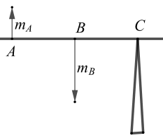
The identity defining can be rewritten more symmetrically:
If points and are equipped with masses and whose sum is equal to zero, then their center of mass is not defined. If is the unit mass, , the corresponding pair is called mass dipole.
Two mass dipoles and are equivalent if the ordered pairs of points and are equal up to a shift.
For the sake of equilibrium of the tabletop, supported at the pivot point , the effect of putting a mass dipole and putting a mass dipole on the tabletop, are equal, if the mass dipoles are equivalent.
Mass dipoles together with weighty points play a key role in the extension of the center of mass technique presented in the paper.
The center of mass of a weighty set containing more than two points can be found inductively using Axiom 2 (see below).
2.2 Axiomatic Definition of the Center of Mass
According to kinematics, centers of mass of weighty sets in a real -dimensional affine space must satisfy the following axioms.
Axiom 1. The center of mass of two points and equipped with masses and with nonzero sum is the unique point on the line such that
Axiom 2. Let be a weighty subset of a weighty set . Let be the center of mass of and let be the total mass of . Then the center of mass of coincides with the center of mass of the set obtained from by replacing the subset by the point equipped with mass .
Theorem 2.1.
There is a unique way of assigning the center of mass to any weighty set of points in a real -dimensional affine space so that Axioms 1 and 2 hold.
We will not prove Theorem 2.1 now. Its classical proof can be described in the following way (see proof of Theorem 2.1, presented right after Lemma 7.7).
One can define the center of mass by an explicit formula and check that the center of mass thus defined satisfies Axioms 1, 2. Uniqueness of the center of mass (see Theorem 2.2 below) implies that the explicit formula provides the unique possible definition of the center of mass and proves its existence.
Theorem 2.2.
Assuming that there is a way of assigning a center of mass to any weighty set of points in a real -dimensional affine space so that Axioms 1 and 2 hold, one can compute the center of mass of any weighty set (in many different ways) using an inductive procedure presented in the proof of Theorem.
Remark 2.3.
Theorem does not imply the existence of a center of mass satisfying Axioms 1, 2: different ways of computation of the center of mass could provide different answers.
Remark 2.4.
Theorems 2.1, 2.2 hold for affine spaces over arbitrary field whose characteristic is not equal to two.These theorems are not applicable to affine spaces over fields of characteristic two (the proof of Lemma 2.5 implicitly uses division by two and it does not work over fields of characteristic two). Our extension of the center of mass technique works for affine spaces over arbitrary fields.
Lemma 2.5.
If a weighty set contains at least two points, then it contains a weighty subset of two points.
Proof 2.6.
If all subsets of containing two points are weightless, then weights of all points are equal up to sign. A triple of such weighty points contains a pair of weighty points equipped with equal masses. This pair of points is a weighty subset of .
Proof 2.7 (Proof of Theorem 2.2).
Using Axioms 1, 2 one can compute the center of mass of any weighty set of points. Indeed:
-
•
Axiom 1 allows to compute the center of mass for any weighty set containing two points;
-
•
by Lemma 2.5, a weighty set containing at least two points, contains a weighty pair of points. By Axiom 2, one can replace this pair of points by its center of mass equipped with its total mass;
-
•
the above properties allow to find the center of mass of a weighty set recursively, by reducing it to computation of the center of mass of weighty sets, containing smaller number of points;
Theorems 2.1, 2.2 have countless applications in geometry: Theorem 2.1 implies that all the different ways of finding the center of mass of a given weighty set, suggested by Theorem 2.2, have to give the same answer.
Classical applications of centers of mass in geometry are based on the above statement.
Let us present the simplest classical application of centers of mass in geometry which goes back to Archimedes.
2.3 Three Medians in a Triangle (Archimedes)
Let us prove the theorem on three medians in a triangle using the center of mass technique. A similar proof was discovered by Archimedes who invented the center of mass technique in geometry.
Suppose we start with a triangle and three unit mass at its vertices. How can we find the center of mass of the resulting system?
One way is to combine masses at and first. This will give us mass 2 placed at the midpoint of .
Now, combine the resulting mass with the unit mass at . By doing so, we obtain that the center of mass lies on the segment connecting the vertex to the midpoint of and divides it in the proportion (the part of it adjacent to the vertex being the longer one).
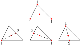
But we could proceed differently: first, combine the masses at and , and then combine the result with the mass at . In this way we obtain that the center of mass of the system lies on the median from vertex and divides it in the ratio .
By combining the masses in the third possible order ( and first and adding afterwards), we see that it also lies on the median from the vertex and divides it in the ratio .
Thus, the center of mass lies on all three medians of triangle and divides them in the ratio . We proved that all three medians of the triangle pass through a point which divides them in the ratio .
3 How to Improve the Center of Mass Technique?
The classical center of mass technique has the following disadvantage: the center of mass is not defined for weightless sets.
One is tempted to look for a commutative group of weighty points in with the following addition: the sum of weighty points is equal to the center of mass of the set of these points, equipped with its total mass.
Unfortunately, such a group does not exist: the sum of weighted points whose total mass is equal to zero, is not defined.
3.1 The Group of Weighty Points and Mass Dipoles
It is possible to improve the center of mass technique and to define a commutative group whose elements are weighty points in and mass dipoles in , defined up to a shift.
Instead of the center of mass, one can assign to any weightless set its mass dipole, defined up to a shift (one can identify a mass dipole , defined up to a shift, with the free vector, represented by an ordered pair of points , defined up to a shift).
Addition in the group satisfies the following condition: the sum of points, contained in a set , whose total mass is , equals to the center of mass of , equipped with the mass .
Addition in the commutative group could be defined axiomatically. Instead of one axiom, describing the center of mass of a weighty pair of points, one has to introduce four axioms, describing the following four different types of addition in :
-
•
addition of two weighty points whose total mass is not equal to zero;
-
•
addition of two weighty points whose total mass is equal to zero;
-
•
addition of a weighty point and a mass dipole defined up to a shift;
-
•
addition of two mass dipoles defined up to a shift.
Numerous geometric applications of the group are based on its associative property:
addition of elements of the group performed in different orders gives the same answer.
Along with classical applications dealing only with the centers of mass of weighty sets, there are many natural applications, that use weightless sets and their mass dipoles as well. To show how it works, we describe one simple geometric application of the group (see Section 8).
Below we define the group for any affine space over an arbitrary field . Moreover, we show that the group admits a structure of a vector space over the field .
The vector space can be naturally identified with the space of moment-like maps of the affine space to the space of free vectors in . We deduce properties of the group from the corresponding properties of the additive group of .
The definition of moment-like maps is motivated by kinematics. In the next section, we discuss a heuristic equilibrium criterion which suggests an explicit formula for the center of mass of a weighted set of points. It allows to justify the classical center of mass technique. It also leads to definitions of moment maps of weighted sets, of moment-like maps and of group .
3.2 Moments of Weighted Sets about Pivot Points and Moment Maps
Imagine a weightless tabletop with a weighted set of points on it. Assume that the tabletop is supported by one leg at a point .
Definition 3.1.
The moment of a weighted set about a pivot point is a linear combination of oriented segments (which we consider as free vectors in ) with coefficients .
| (1) |
Kinematics suggests a simple criterion of stability of the tabletop with the set on it, supported at a point .
Kinematical Criterion. The tabletop is in equilibrium if and only if the moment of about the pivot point equals zero.
Only the moment of the set about the pivot point is important for the equilibrium of a tabletop supported at : for the sake of equilibrium of the tabletop supported at , the effects of putting a weighted set and putting a weighted set on the tabletop are equal if the moments of and about the point are equal.
Definition 3.2.
The moment map corresponding to a weighted set is the map , whose value at a point is equal to the moment of the set about the pivot point .
Theorem 3.3 (Change of pivot point).
Let be the moment map, corresponding to a weighted set whose total mass is equal to . Then, for any two points , the map satisfies the following characteristic relation:
| (2) |
Definition 3.5.
A moment-like map is a map of the affine space to the vector space of free vectors on that satisfies the relation (2) for some parameter . The parameter , which depends on the map , is called the total mass of the map .
It is easy to see that the set of all moment-like maps has a natural structure of a vector space, and the total mass is a linear function on .
Applying Theorem 6.19, one can check that, if the total mass of a map does not equal to zero, then vanishes at a unique point called the center of mass of the map . Such a map is uniquely determined by its center of mass and its total mass (see Theorem 6.21).
Moreover, the map is equal to the moment map of the weighty set consisting of one point equipped with the mass .
Equation (2) implies that, if the total mass of a map equals zero, then is a constant map, i.e., , where is a free vector. The map is determined by the free vector .
Lemma 3.6.
The moment map of a mass dipole is a constant map , where is the free vector represented by an ordered pair of points .
Proof 3.7.
The moment of about a pivot point is equal to the difference of oriented segments and , considered as free vectors. This difference is equal to the oriented segment which can be considered as the free vector , represented by an ordered pair of points .
Let us introduce the following identifications:
-
•
a moment-like map with total mass is identified with the weighty point , where is the center of mass of ;
-
•
a constant moment-like map is identified with a mass dipole , defined up to a shift, the ordered pair of points represents the free vector .
By this identification, we obtain a vector space whose elements are weighty points and mass dipoles, defined up to a shift. The additive group of the space can be defined by the axioms which define the addition in the set .
Let us implement this program in more details.
4 Affine Spaces and Affine Maps
Below, we recall that Euclidean spaces, vector spaces over an arbitrary field and shifted vector subspaces in such spaces can be considered as affine spaces.
4.1 Vector Space of Free Vectors in a Euclidean Space
Classical Euclidean geometry, in particular, deals with points, lines and planes embedded in the three dimensional space. These objects are Euclidean spaces of dimensions zero, one, two and three.
A Euclidean space does not have a structure of a real vector space: an operation of multiplication of a point by a real number and an operation of addition of two points are not defined.
Nevertheless, to any Euclidean space one can assign a real vector space of free vectors in and define an action of the additive group of free vectors on the space .
Let us define free vectors in a Euclidean space .
Definition 4.1.
Two ordered pairs of points and from the space are equivalent , or are equal up to a shift, if the oriented segments and are parallel, equal in length and point in the same direction.
Definition 4.2.
A free vector in is an ordered pair of points in , defined up to the equivalence .
One can multiply an ordered pair of points by any real number . By definition, is an ordered couple of points such that the points belong to the same line, and ratio of oriented length of the segments and equals .
It is easy to check that if , then .
Definition 4.3.
Let be an ordered pair of points that represents a free vector . Then, by definition, is the free vector represented by the ordered pair .
One can add any two ordered pairs of points and . By definition, is an ordered pair of points such that the oriented segments and are parallel, equal to each other and point to the same direction.
Easy to check that if and , then .
Definition 4.4.
Let , be ordered pair of points which represent free vectors . Then, by definition, is the free vector represented by the oriented pair .
One can verify that if in an -dimensional Euclidean space (), then the space of free vectors in is an -dimensional real vector space.
There is a natural operation of addition for a free vector and a point in the space . The result of such addition is a point in the space .
One can add a vector to a point.
Definition 4.5.
By definition, a point is the sum of a point and a free vector if the ordered pair of points represents the free vector .
It is easy to check the following lemma.
Lemma 4.6.
Let be any point in . Then
-
1.
the identity holds if and only if is the zero vector in the space of free vectors ;
-
2.
for the identity holds.
-
3.
for any point , there is a unique free vector such that .
A free vector defines the shift of the space that maps a point to the point .
Lemma 4.6 implies that the shifts constitute the action of the additive group of free vectors on the space . Moreover, this action is transitive and free.
Remark 4.7.
Euclidean geometry equips the vector space of free vectors in with the inner product of vectors . The inner product is a symmetric bilinear form in the vector space that is positively defined, i.e., and only if . The inner product allows defining distances between points and angles between lines in a Euclidean space .
4.2 Vector Spaces as Affine Spaces
Let be a vector space over an arbitrary field . In this section, we define the structure of an affine space on , i.e., we define the vector space of free vectors in and the action of the additive group of free vectors on the space .
Definition 4.8.
A shift of the space by a vector is the map which sends a point to the point .
The additive group of the vector space acts on the space by shifts: a vector sends a point to the point .
Definition 4.9.
A free vector in is an ordered pair of points defined up to a shift (i.e., for any the ordered pair of points defines the same free vector as the ordered pair of points ).
One can identify a free vector , represented by a pair , with the vector . By definition, the vector is well defined, i.e., is independent of a choice of a pair , that represents the free vector .
Definition 4.10.
By definition, a vector space operation on the space of free vectors is induced from the corresponding vector space operation on the vector space under the identification of with the vector space .
Thus, we defined the vector space of free vectors in . The action of the additive group of on is defined as follows: a free vector sends a point to the point .
4.3 Shifted Vector Subspaces as Affine Spaces
An affine subspace is a vector subspace shifted by a vector . In general, if does not belong to , the space is not a vector space. Instead, it can be naturally equipped with a structure of an affine space, i.e., with a vector space of free vectors on and with an action of the additive group of free vectors on the space .
We define an affine structure on using vector space operations in the ambient space .
Definition 4.11.
A set is a shifted subspace by a vector if , i.e., if each point is representable in the form , where . (In other words, the set is a coset of the additive group of the vector subspace , containing the point .)
Definition 4.12.
Two ordered pairs of points and in an affine space are equivalent if . (In other words, the pairs are equivalent if they define the same free vector in the ambient space .)
A free vector in an affine space is an equivalence class of ordered pairs of points in .
There is a natural embedding of the set to the vector space which sends a free vector in , represented by an ordered pair of points from , to the free vector in represented by the same ordered pair of points .
Lemma 4.13.
Each free vector as a free vector in has a unique representative of the form , where is the origin of the vector space , and belongs to the vector space .
Proof 4.14.
Indeed, a free vector in is equivalent to a unique ordered pair of points of the needed form.
One can identify a free vector , represented by a pair with the vector . The vector is well defined, i.e., is independent of a choice of a pair which represent the free vector .
Definition 4.15.
By definition, a vector space operation on the space of free vectors in is induces from the corresponding vector space operation on the space under the identification of with the vector space .
Thus, we defined the vector space . The action of the additive group of on is defined as follows: a free vector sends a point to the point . The vector space is naturally embedded in the vector space and the actions of the additive groups of these spaces on agree with this embedding.
Let us choose any point in an affine space and identify a point with the free vector , such that (in other words, one identifies a point with the free vector , represented by the ordered pair of points .
This identification provides an affine space with the structure of a vector space whose origin is the point . Different choices of the origin provide with different structures of vector spaces .
For any point , the affine space can be considered as an affine subspace in the vector space (which as a set coincides with ). The affine structures induced in as a subset of are the same for different choices of the point :
-
1.
vector spaces of free vectors in different spaces can be naturally identified with each other;
-
2.
identified free vectors from different spaces realize the same action on the space .
The center of mass technique deals with affine spaces over arbitrary fields. In particular, it is applicable to -dimensional Euclidean spaces which are real dimensional affine spaces equipped with an extra structure.
In the next section, we briefly recall the definition of multidimensional Euclidean spaces. We will not use this definition later.
4.4 Multidimensional Euclidean Spaces
One can assign the structure of an affine space to any vector space : as a set, the affine space coincides with the vector space , the space of free vectors in the affine space and the action of the additive group of free vectors on the affine space have been defined above.
The real -dimensional affine space is, by definition, the affine space associated with the real -dimensional vector space .
An -dimensional Euclidean space is a real -dimensional affine space equipped with a positive definite quadratic form on the vector space of free vectors on .
Using a positive definite quadratic form on , one can define distances between points, angles between lines in , and develop geometry based on this notions in .
For this geometry can be identified with the classical Euclidean geometries of corresponding dimensions.
Euclidean geometry in the spaces of dimension is a natural and rich generalization of classical Euclidean geometry.
4.5 Affine Maps
Let and be affine spaces over a field . A map sends an ordered pair of points in to the ordered pair of points in .
Definition 4.16.
A map is an affine map if:
-
•
the induced map is well defined, i.e., if the pairs and define the same free vector in , then the pairs and define the same free vector in ;
-
•
the induced map is a linear map.
Let us choose some points and and consider affine spaces and as the vector spaces and .
Definition 4.17.
A map is a shifted linear map if it can be represented in the form
where is an arbitrary linear map (which is called the linear part of ), is an arbitrary vector, and is any point in the vector space .
Theorem 4.18.
The map is an affine map if and only if, for any choice of points , it gives rise to a shifted linear map of to .
Moreover, the linear part of the map can be naturally identified with the linear map , which is independent of choice of points and .
Proof 4.19.
Assume that is an affine map. By definition, induces a linear map . Let us identify the space with the space and the space with the space . Under this identification, the map can be considered as a linear map . Let be a point . Then the map can be identified with the map from to
Conversely, any map of to , where is a linear map and is an arbitrary vector in , obviously, gives rise to an affine map of to .
Corollary 4.20.
The space of polynomials of degree on coincides with the space of affine maps of an affine space to the one dimensional affine space .
Proof 4.21.
In the vector space with the origin at a point , a function is a polynomial of degree if it can be represented as , where is a linear function, and is a constant. Thus, is a polynomial of degree if and only if it is a shifted linear map of to .
One can automatically verify the following two lemmas.
Lemma 4.22.
Let be an affine space over , and let be a vector space over . Then the space of affine maps is a vector space over , i.e., the sum of affine maps and the product of affine map on are affine maps.
Lemma 4.23.
Let be affine spaces over and let and be affine maps, then:
-
1.
the composition is an affine map;
-
2.
the linear part of the composition is the composition of the linear parts and of the maps and .
It is easy to verify the following theorem.
Theorem 4.24.
An affine map is invertible if and only if its linear part is invertible.
All invertible affine maps of an affine space to itself form a group under composition.
Definition 4.25.
The group of affine transformations of an affine space is the group of all invertible affine maps .
Remark 4.26.
According to Felix Klein’s Erlangen program, in affine geometry of an affine space , two subsets , are considered as equal sets if there is an affine transformation of which sends the set to the set .
Affine geometry studies properties of sets, which are preserved under affine transformations (i.e., which are the same for equal sets).
5 Weighted Sets and their Moment Maps
In this section, we discuss weighted sets in an affine space , their moments about a pivot point and their moment maps.
5.1 The Vector Space of Weighted Sets
In this section, we define the vector space of finite sets of points in equipped with weights from the field . The definition does not rely on the affine structure of and can be applied to any set .
Let be an affine space over an arbitrary field .
Definition 5.1.
A weighted set in is a finite set of points in equipped with elements of the field . The element is the mass assigned to the point . The total mass of a weighted set is the element equal to the sum of masses of all points in the set.
The set off all weighted sets in has a natural structure of a vector space over the field . Indeed, one can interpret a weighted set as a function which vanishes on and whose value at each point is equal to .
Definition 5.2.
The space is the vector space over of all functions on , taking values in the field and equal to zero everywhere but on a finite set of points. A weighted set can be identified with the function . This identification provides the set with the structure of a vector space over .
Example 5.3.
A partition of a weighted set is a representation of the set as a union of its disjoint subsets equipped with the masses induced from the weighted set.
If weighted subsets and of a weighted set realize its partition, then the weighted set is the sum of the weighted sets and .
A function , which assigns to a weighted set its total mass, is a linear function on the space .
Definition 5.4.
A weighted set in with total mass is called:
-
1.
a weighty set if its total mass is not equal to zero;
-
2.
a weightless set if its total mass is equal to zero.
Definition 5.5.
Let us denote by the subset of the set that consists of all weightless sets in .
Since the total mass of a weighted set is a linear function on the vector space , the set of weightless sets is a vector subspace of codimension one in .
5.2 The Moment of a Weighted Set
One can repeat almost verbatim definitions of the moment about a pivot point and of the moment maps of weighty sets in an affine space over an arbitrary field (see below).
Definition 5.6.
The moment of a weighted set about a pivot point is a linear combination of the free vectors with coefficients :
| (3) |
The following Theorem is obvious:
Theorem 5.7 (Linearity of moment).
For each pivot point , the moment of a weighted set about the pivot point gives a linear map of the space to the space of free vectors in .
Proof 5.8.
To prove the theorem one has to check that:
-
1.
if , then, for every point , the identity holds;
-
2.
if for , then, for every point , one has
One can easily verify each of these statements.
Corollary 5.9.
For any partition of a weighted set into a union of weighted subsets, the moment of the set about any pivot point is equal to the sum of the moments of the subsets about the same pivot point.
Definition 5.10.
Two weighted sets and are equivalent, i.e., if their moments about any pivot point are equal. A weighty set in is a null set if its moment about any pivot point is equal to zero. Denote the set of all null sets in by .
By definition, two sets and are equivalent if is a null set.
Theorem 5.7 implies the following corollary.
Corollary 5.11.
The set of all null sets in is a vector subspace of the vector space . The equivalence of weighted sets respects the linear operations on weighted sets, i.e., the following relations hold:
-
1.
if , then for any ;
-
2.
if are , then .
Definition 5.12.
The moment map of a weighted set is the map which sends a point to the moment of the set about the pivot point .
The following theorem repeats Theorem 5.13 almost verbatim and can be checked in the same way.
Theorem 5.13 (Change of a pivot point).
Let be the moment map corresponding to a weighted set , whose total mass is equal to . Then, for any two points , the map satisfies the following relation:
| (4) |
6 The Space of Moment-like Maps and the Space of Weighty Points and Mass Dipoles
In this section, we study the space of moment-like maps and define the space of weighty points and mass dipoles in an affine space over an arbitrary field .
6.1 Moment-like Maps
In this section, we will study a special class of affine maps which plays a key role for the center of mass technique.
Definition 6.1.
An affine map of an affine space over a field to the vector space of free vectors in is a moment-like map if its linear part is equal to , where is the identity map and is a parameter called the total mass of and denoted by . Denote by the collection of all moment-like maps of an affine space to the vector space of free vectors on .
The definition implies that a map is a moment-like map with total mass if and only if, for any two points , the following characteristic identity holds:
| (5) |
Lemma 6.2.
The set of all moment-like maps of an affine space over a field is a vector space over , i.e., the sum of two moment-like maps of is a moment-like map of ; the product of a moment-like map of on an element is a moment-like map of .
The function , which assigns to a map its total mass , is a linear function on .
Proof 6.3.
For each fixed pair of points the characteristic identity can be considered as a linear homogeneous equation on a map . Solutions of any system of linear homogeneous equations form a vector space.
Linearity of the function is also a straightforward consequence of definitions.
The characteristic identity can be rewritten in the following form:
| (6) |
Formula (6) immediately implies the following theorem.
Theorem 6.4.
The total mass of a map is equal to zero if and only if is a constant map , where . The space of all maps , whose total mass equals to zero, is a vector subspace in of codimension one. The map , that sends to the free vector , is a natural isomorphism between the space and the space .
Proof 6.5.
According (6), a map is a constant map if and only if its total mass is equal to zero. The total mass is a linear function on . Thus, the equation defines a vector subspace of whose codimension is one.
The second statement of the theorem is obvious.
Lemma 6.6.
A constant map is the moment map of a mass dipole such that the ordered pair of points defined up to a shift, represents the free vector .
Proof 6.7.
The lemma can be proven in almost the same way as Lemma 3.6.
Lemma 6.8.
There is a unique map , whose total mass is a given element and whose value at a chosen point is a given free vector .
Proof 6.9.
According to (6), the value of the map at a point is equal to .
Conversely, the map defined by the formula satisfies the assumption of the lemma.
Corollary 6.10.
The vector space is isomorphic to the direct sum (an isomorphism is not canonical).
Proof 6.11.
Fix a point . The map that sends a map to the pair for each point , provides an isomorphism between and . This isomorphism depends on the point and is not canonical.
Corollary 6.12.
The dimension of the space is equal to the dimension of the space plus one, i.e., the dimension of the space is equal to .
Definition 6.13.
Let be a map whose total mass is not equal to zero. The center of mass of the map is a point at which the map vanishes, i.e., .
Definition 6.14.
The normalized map of a map whose total mass is not equal to zero, is the map .
Lemma 6.15.
A map with nonzero total mass and the normalized map vanish at the same point. The normalized map has the total mass 1.
Proof 6.16.
Two proportional vector-valued functions and vanish at the same points. The total mass is a linear function on the space . The total mass of the normalized map is equal to .
Theorem 6.17.
Assume that the total mass of a map is equal to . Then, for any point , the free vector sends the point to the point which is independent of the point .
Moreover, the point is the unique point at which the function vanishes.
Proof 6.18.
Indeed, for any two points the characteristic identity can be rewritten in a following form: . Thus, the points and are mapped by the free vectors and to the same point .
The point itself has to be sent to the point , so that which implies that . For any other point , we have . Thus, . The theorem is proven.
Theorem 6.19.
Assume that the total mass of a map is not equal to zero. Then has a unique center of mass . For any point the following relation holds: the free vector sends the point to the center of mass , i.e.,
| (7) |
Moreover, if the affine space has a structure of a liner space , then the vector satisfies the following relation:
| (8) |
where is the zero in the space .
Proof 6.20.
Theorem 6.21.
A map with nonzero total mass is uniquely determined by its center of mass and by its total mass .
Moreover, for any point , the following identity holds: . Thus, is the moment map of the set consisting of one point equipped with mass .
Conversely, the moment map of the set has total mass and center of mass .
Proof 6.22.
Two maps from the space having the same center of mass and the same total mass coincide, since their values at the point are equal, and their total masses are the same.
The point , obviously, is the center of mass of the map given by the relation , and total mass of is .
Lemma 6.23.
If two maps are equal at two different points , then they are equal identically.
Proof 6.24.
Indeed, any non-zero map vanishes no more than at one point. The maps vanishes at two different points and . Thus, is identically equal to zero.
6.2 The Space and the Space of Weighted Sets in
In this section, we show that the space of moment-like maps is isomorphic to space of equivalence classes of weighted sets, i.e., is isomorphic to the space (see Corollary 5.11).
Definition 6.25.
The moment correspondence is the map which sends each weighted set to its moment map .
The kernel of the moment correspondence is the space of null sets in . It is easy to see that a weighted set is a null set if and only if its total mass and its mass dipole are equal to zero.
Theorem 6.26.
The moment correspondence is a surjective map, i.e., any moment-like map is a moment map of some weighted set . The space is isomorphic to a factor-space of the space by its subspace .
Proof 6.27.
Assume that the total mass of a moment-like map is not equal to zero, and its center of mass is a point . Then, by Theorem 6.21, , where consists of one point equipped with mass .
Assume that the total mass of a moment-like map is equal to zero, that is is a constant map . Then, by Lemma 6.6, , where is a mass dipole , where is an ordered pair of points that represents the free vector .
Thus, the correspondence map is onto. Since its kernel is the space of null sets in , the space is isomorphic to the factor-space .
7 The Space of weighty Points and Mass Dipoles in
Let be an affine space over an arbitrary field . In this section, we define the vector space over of weighty points and mass dipoles in . The additive group of that vector space has many applications in geometry.
The space can be interpreted as the factor-space of the space of weighted points in by its subspace of all null sets in . Our presentation is based on the isomorphism between the spaces and discussed above and on the properties of the space .
Definition 7.1.
A weighty point in is the point equipped with a nonzero mass .
Definition 7.2.
A mass dipole in is an ordered pair of points in equipped with masses respectively. Two mass dipoles and are called equal if the ordered pairs of points and are equal up to a shift.
By definition, a mass dipole can be identified with a free vector, represented by the ordered pair of points in . The class of the empty set can in be considered as a mass dipole or as the zero free vector.
Definition 7.3.
The set defined as the set of all weighty points in and all mass dipoles in defined up to a shift.
There is a natural one-to-one correspondence between the sets and (see Definition 7.5 below).
The correspondence allows to identify the sets with the space and to define a structure of a vector space on the set .
Definition 7.4.
The structure of a vector space over on is the structure induced by the identification from the -vector space structure on .
The above definition implies that the vector space operations on the set are defined as follows. To perform a vector space operation on points from the set one has to:
-
•
identify the points in with the maps from the space ;
-
•
perform the desired vector space operation on the maps from , and
-
•
identify the map, obtained as the result of this operation, with a point of .
We will specify vector space operation on the space in Section 7.1. Now we will define the one-to-one correspondence .
The space contains maps of two types: maps of the first type whose total mass is a nonzero element of the field , and maps of the second type whose total mass is equal to zero.
Each map of the first type is uniquely determined by its center of mass and by its total mass .
Each map of the second type is a constant map , where is a free vector represented by an ordered pair of points defined up to a shift.
We now define the map .
Definition 7.5.
The map sends a weighty point to the map of first type whose total mass is and whose center of mass is the point .
The map sends a mass dipole to the map , of the second type, where is a free vector, corresponding to an ordered pair of points .
Now, that vector space operations on the set are defined, one can describe each type of vector space operation separately, see lemmas in Section 7.1 below. Each of these lemmas can be easily verified. The content of the lemmas can be considered as an axiomatic definition of the space . The additive group of the space is important for geometrical applications.
Since the set contains points of very different nature, definition of addition is a bit tricky: addition of different types of pairs of points in is performed by different rules. Because of that, the associativity of addition is not obvious.
Geometrical applications of the additive group come from the following statement:
The sum of several elements of the group is well defined: it does not depend on order in which the addition of pair of elements is performed.
7.1 The Vector Space Operations on
Let us describe vector space operation on the space .
Lemma 7.6.
The product of a weighty point by , is the weighty point if , and is a zero mass dipole if . The product of a mass dipole , corresponding to a free vector , by , is the mass dipole, corresponding to the free vector .
In geometrical applications, the additive group of the space plays a key role. Let us give more detailed description of addition in .
Lemma 7.7.
The sum of two weighty points and with is the weighty point , where is a point such that the free vectors and are proportional and their ratio satisfies the relation
| (9) |
Proof 7.8.
By definition, the center of mass of the weighty set defined in the statement of the lemma, is a point such that , or which is equivalent to (9).
If is a real affine space, then Lemma 7.7 implies that the oriented segments and are proportional and
Lemma 7.7 implies that the point as a vector in a vector space containing the affine space , satisfies the following relation:
Let us justify the classical center of mass technique.
Proof 7.9 (Proof of Theorem 2.1).
We have to prove that there is a way of assigning the center of mass to every weighty set that satisfies Axioms 1, 2. The uniqueness of such center of mass is proved above (Theorem 2.2). Above, we defined the center of mass of a weighty set as the only point where the moment map vanishes. Lemma 7.7 implies that the center of mass defined in such a way satisfies Axiom 1. It satisfies Axiom 2, since the moment map , by Theorem 5.7, depends linearly on the weighted set .
The next three lemmas describing other types of addition in the group , are also straightforward. We will nor present their proofs.
Lemma 7.10.
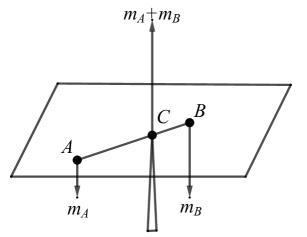
The sum of a weighty point and a mass dipole is the weighted point , where the point is the sum of the point and the free vector .

If is a real affine space, then the lemma implies that the oriented segments and are parallel, equal and point to the same direction (see Figure 5).
The lemma implies that the point as vectors in a vector space containing an affine space , satisfy the following relation:
Lemma 7.11.
The sum of two mass dipoles and is the mass dipole that corresponds to the free vector .
If is a real affine space, then the lemma implies that the oriented segments (which we consider us free vectors defined up to shifts) satisfy the following relation:
The lemma implies that the points as vectors in a vector space containing an affine space , satisfy the following relation:
Lemma 7.12.
The sum of two weighted points and is the mass dipole that corresponds to the free vector .
If is a real affine space, then the lemma implies that the oriented segments , defined up to a shift, satisfy the following relation:
The lemma implies that the points as vectors in a vector space containing an affine space , satisfy the following relation:
8 The Orthocenter and the Euler Line
In this section, we give a simple application of the extended center of mass technique (in other words, of the additive group ). We will prove the following classical results:
-
1.
the three altitudes of a triangle have a common point; it is called the orthocenter;
-
2.
for any triangle, its orthocenter , its barycenter (i.e., the intersection points of its medians) and its circumcenter (i.e., the center of a circle, passing through all the vertices of the triangle) belong to one line (which is called the Euler line of the triangle). Moreover, the relation holds.
8.1 The Three Altitudes of a Triangle and Masses
Applying the extended center of mass technique, one can show that the three altitudes of a triangle pass through a common point (which is called the orthocenter of the triangle). Moreover, one can see how the orthocenter is located at each of these altitudes (see Theorem 8.3).
Consider a triangle . Let be the center of the circle passing through the vertices .
Consider a weighted set containing the points , in which the points have mass and the point has mass .
Let us compute the center of mass of the set in several different ways.
Let be the altitude of passing through the vertex and let be the midpoint of the side .
Lemma 8.1.
Denote by the point on the line such that the oriented segment is equal to the oriented segment multiplied by two, i.e., . Then the point is the center of mass of weighty set .

Proof 8.2.
Partition into two subsets: and .
The sum of the masses of the points is equal to zero. The mass dipole of these weighted points is equal to the sum of vectors which is equal to the vector . Since the point has mass , the center of mass of the set is at the point shifted by the vector (see Lemma 7.10). Thus, it is equal to the point .
In the same way, one can compute the center of mass of the set by its subdividing it into two weighted subsets: a weighty vertex of the triangle and a weightless set complimentary to the vertex. Since the center of mass is well defined, we obtain the following result.
Theorem 8.3 (The three altitudes theorem).
In a triangle the three altitudes pass through a common point . Moreover, for any vertex (where is , or ), the vector is equal to , where is the midpoint of the side opposite to the vertex .
8.2 The Euler line of a Triangle and Masses
In the previous section, we considered the weighty set consisting of the vertices of a triangle equipped with the unit masses and the center of the circle passing through the vertices equipped with mass . We proved that the center of mass of the set is the orthocenter . In the proof, we used three different subdivisions of the set .
Let us subdivide in a fourth way and apply this subdivision to another computation of the center of mass of . It will allow us to prove a beautiful Euler line theorem for the triangle .
Let be the orthocenter of the triangle , i.e., the point of intersection of its three altitudes.
Let be the barycenter of the triangle , i.e., the point of intersection of its three medians (see Section 2.3).
Let be circumcenter of the triangle .
Theorem 8.4 (The Euler line).
For any triangle , the points are collinear. Moreover, the point divides the segment in proportion , i.e.,
Proof 8.5.
Let us subdivide the weighted set into weighted sets and . Instead of the weighted set , one can take its center of mass equipped with mass . Thus, the center of mass of is equal to the center of mass of the weighted set , where has mass and has mass .
From the properties of the center of mass, we conclude that
We also have the following relations:
These identities imply the theorem.
9 Affine Hyperplanes not Passing Through the Origin in a Vector Space
In this section we discuss geometry of an affine hyperplane not passing through the origin in a vector space. We also show that any affine space can be canonically embedded into a vector space as an affine hyperplane not passing through the origin.
9.1 Affine Transformations of a Hyperplane and Linear Transformations of the Ambient Space
In this section, we discuss a natural relation between affine geometry of hyperplane, not passing through the origin, and linear algebra of the ambient vector space.
Let be an affine hyperplane in a vector space not passing through the origin of . Let be a vector subspace parallel to . The space can be naturally identified with the vector space of free vectors in the hyperplane .
Theorem 9.1.
Any affine map extends to a unique linear map . The affine space and the vector space are invariant subspaces for .
Conversely, let be a linear map such that is invariant under . Then the restriction of to is an affine map .
Proof 9.2.
The space of free vectors in can be identified with the space . Under this identification, the linear part of an affine map becomes a linear map . Let us define as the linear map whose restriction to is equal to and whose value at a chosen vector is equal to the vector .
It is easy to see that the linear map , thus defined is an extension of . The uniqueness of an extension is obvious, since any vector in can be represented as a linear combination of vectors from .
Conversely, it is easy to see that the restriction of to an invariant subspace is an affine map .
Definition 9.3.
Let be the subgroup of the group consisting of invertible linear transformations of under which the hyperplane is invariant.
Theorem 9.4.
The restriction of a transformation to the is an affine automorphism of . Any affine automorphism of is the restriction of a unique linear transformation .
Proof 9.5.
The theorem follows from Theorem 9.1. We only have to show that if an affine map is invertible, then its extension also is invertible.
Indeed, the linear part is invertible. Thus, the restriction of to the invariant subspace is invertible. The dimension of the factor-space is equal to one, and the image of spans the space . The map induces the identity transformation the factor-space , since it sends to . Thus, is an invertible map.
Remark 9.6.
According to Felix Klein’s Erlangen program, geometry of an affine space is determined by the group of affine transformations of the space .
Theorem 9.7.
Any polynomial of degree on an affine hyperplane in a vector space can be uniquely extended to linear function on the space .
Conversely, the restriction of any linear function on to is a polynomial of degree .
Proof 9.8.
A polynomial of degree on an affine space is an affine map . The linear part is a linear function on which can be considered as a linear function on the space . Let us choose any point . An extension can be constructed as the linear function on that coincides with on the and whose value a chosen point is .
The uniqueness of linear extension is obvious, since any vector from can be represented as a linear combination of elements of .
Corollary 9.9.
One can naturally identify the ambient vector space with the vector space dual to the space of degree polynomials on .
Proof 9.10.
Theorem 9.7 allows to canonically identify the space with the space dual to the space . This identification canonically identifies the space dual to the space with the space .
9.2 Canonical Realization of an Affine Space as a Hyperplane in Vector Space
Let us describe a canonical realization of an affine space as a hyperplane, not passing through the origin, in a vector space.
We will need a general definition of Kodaira’s map. Let be a set, and let be a space of functions on taking values in a field .
Definition 9.11.
Kodaira’s map is the map of to the dual space that sends a point to the linear function on whose value at is equal to .
Lemma 9.12.
Kodaira’s map is an embedding if separates points in , i.e., for any points in , there is a function such that .
Proof 9.13.
If separates points , then Kodaira’s map sends and to different linear functions on , since their values at the function are different.
Definition 9.14.
Assume that the space contains a constant function for any . A characteristic hyperplane is a hyperplane consisting of all linear functions on whose value at the function is equal to .
Lemma 9.15.
Assume that the space contains all constant functions on . Then Kodaira’s map sends to the characteristic hyperplane of the space .
Proof 9.16.
The value of the function at each point is equal to .
Set , an affine space, and .
Lemma 9.17.
Kodaira’s map is an affine map.
Proof 9.18.
A polynomial of degree is an affine map . Its linear part is a linear function on the space of free vectors in . Thus, the difference is invariant under all translations of the pair (i.e., if , then ) and depends linearly on the free vector . These properties imply that Kodaira’s map is an affine map.
Theorem 9.19.
Kodaira’s map provides a canonical affine embedding of the affine space to the vector space . The image of under the embedding coincides with the characteristic hyperplane in the space .
Proof 9.20.
By Lemma 9.12, the map is an embedding, since all constant functions on are polynomial of degree . By Lemma 9.17, the map is affine; by Lemma 9.15, it maps to the characteristic hyperplane . The dimension of the characteristic hyperplane is equal to the dimension of . Indeed, . Thus, the map provides an isomorphism between the affine spaces and .
10 Several Interpretations of the Space of Weighty Points and Mass Dipoles
In this section, we show first that an affine map induces the linear map . Then we give three interpretations of the space .
10.1 A Linear Map of the Space of Weighty Points and Mass Dipoles Induced by an Affine Map
Let be affine spaces over a field , and let , be vector spaces over of sets of weighted points in and correspondingly. Consider any map .
Definition 10.1.
The map induced by the map is the map that sends any single point , equipped with mass 1, to the single point equipped with mass 1, and which extends the above map by linearity to the space .
The definition implies the total mass of the set in and in are equal. Thus, the following inclusion holds:
The definition of the map does not use affine structures on and (and it could be applied to vector spaces of weighted points in any sets and ). The following Lemma uses the affine structures on and in a very essential way.
Theorem 10.2.
If is an affine map, then takes the null sets in to null sets in .
Proof 10.3.
Let be a set of points equipped with masses . Since is a null set, its total mass is equal to zero, and, for any point , the free vector is equal to zero. Thus, is the zero free vector in . It implies that the free vector equals to zero. Thus, the moment of the set about the point equals to zero. Since the total mass of the set is zero, the set is a null set.
Corollary 10.4.
If is an affine map, then the map is a well defined linear map.
Proof 10.5.
By Theorem 10.2, the linear map takes the subspace of null sets in to the subspace of null sets in . Thus, induces a well defined linear map from the factor-space to the factor-space .
Corollary 10.6.
Let be an affine map. If is a weighty set in with nonzero total mass and the center of mass , then the set is a weighty set in with nonzero total mass and the center of mass .
If is a weightless set in whose total mass equals to zero and whose mass dipole is , then the set is a weightless set in whose total mass equals to zero and whose mass dipole is .
Proof 10.7.
If two weighted sets in are equivalent in , then their images under the map are equivalent in , since maps null sets in to null sets in .
If a weighty set in is equivalent to a weighty point , then the set in is equivalent to the weighty point . Thus, the first statement of the Corollary is proved.
If a weightless set in is equivalent to a mass dipole , then the set in is equivalent to the mass dipole . Thus, the second statement of the Corollary is proved.
Corollary 10.8.
If is an affine embedding, then the map is a linear embedding.
10.2 The Space of an Affine Hyperplane in a Linear Ambient Space
In this section, we will consider an affine embedding , where is an affine hyperplane in a vector space not containing the origin of the space . We will show that the vector space of weighty points and mass dipoles in is naturally isomorphic to .
Let be the vector subspace in parallel to the affine hyperplane . It is easy to verify the following lemma.
Lemma 10.10.
If an affine hyperplane does not contain the origin , then there is a unique linear function that is identically equal to on the hyperplane .
Moreover, the function vanishes on the vector space parallel to the affine hyperplane .
To provide an isomorphism between the vector spaces and we define a linear map of the space to the ambient vector space whose kernel is the space of null sets in .
Definition 10.11.
Let be the space of weighted points in a vector space . Then the evaluation map is the map, which sends a weighty set in to the vector .
Lemma 10.12.
The evaluation map sends all null sets in to zero.
Proof 10.13.
Indeed, by definition, the vector is equal to the moment of the set about the origin .
Definition 10.14.
Let be the space of weighted points in an affine hyperplane . Then the -map is the map which is the composition of the map , induced by the embedding and the evaluation map .
Lemma 10.15.
Let be the linear function on that takes value on the affine hyperplane . Then the total mass of a set is equal to .
Proof 10.16.
Indeed, if is a weighty point of mass , then . This relation can be extended by linearity to any set :
The lemma is proven.
Lemma 10.17.
If , then is a null set.
Proof 10.18.
Let be a weighted set in . By definition, its image is the moment of the set about the origin . Thus, if , then the weighted set has zero moment about the pivot point . The total mass of the set is also equal to zero, since . Thus, the weighty set is a null set in . The map is an embedding. Thus, the set as a weighted set in also is a null set.
Theorem 10.19.
The map is an isomorphism between the space of weighty points and mass dipoles of an affine hyperplane not passing through the origin and the ambient vector space .
Proof 10.20.
By Lemma 10.17, the induced map is an embedding. The image of under the map , obviously, contains the hyperplane . The smallest vector space that contains this hyperplane is the space . Thus, the induced map is an embedding and a surjective map. Thus, is an isomorphism between the spaces and .
Consider an affine hyperplane in a vector space not passing through the origin. Let be a set of points in equipped with masses . Let be the total mass of the set . Theorem 10.19 implies the following corollary.
Corollary 10.21.
If , then where is the center of mass of the set .
If , then , where is a mass dipole of the set , and is a well defined vector in the vector space parallel to the affine space .
10.3 The Spaces and are Canonically Isomorphic
Let be an affine space over a field , and let be a vector space of degree polynomials on .
Recall that the Kodaira’s map sends a point to the linear function on which assigns to a polynomial its value at the point .
In Section 9.2, we showed that the map is an affine embedding of to , whose image is the characteristic hyperplane (see Section 9.2) in .
Thus, the Kodaira’s map provides a canonical representation of an affine space as the characteristic hyperplane in the vector space .
Corollary 10.22.
There is a natural identification between the vector space of weighty points and mass dipoles in an affine space and the dual space to the space of polynomials of degree on .
Let be a set of points in equipped with masses , and let be the total mass of the set . Theorem 10.19 and Corollary 10.22 imply the following theorem.
Theorem 10.23.
Consider a linear function on the space which sends a polynomial to . If , then , where is the center of mass of the set and is any polynomial from . If , then , where is a mass dipole of the set , and is any polynomial from the space .
10.4 Differentials of Quadratic Polynomials and the Space of Weighty Points and Mass Dipoles
Consider a vector space over a field as an affine space . Let be a non-degenerate symmetric bilinear form on and let be a space of polynomials on , representable in the form , where is the quadratic form, associated with , is an arbitrary linear function, and are arbitrary constants.
The differential of a polynomial on give rise to the map which assigns to a point the linear function of .
With the space , one can associate the vector space of differentials of all polynomials .
Theorem 10.24.
The vector space of differentials of all polynomials from the space is isomorphic to the space of weighted points and mass dipoles in . Under this isomorphism:
-
1.
a weighty point of a nonzero mass corresponds to the differential of a polynomial whose critical point is the point , i.e., , where is an arbitrary constant;
-
2.
a mass dipole corresponds to the differential of a polynomial of degree , where is the linear function defined by relation .
Consider a polynomial representable in the form
Denote by the set of points equipped with masses . Let be the total mass of the set . The theorem implies the following corollary.
Corollary 10.25.
If , then , where is the center of mass of the set and is some constant.
If , then , where is the linear function defined by relation , where is the mass dipole of the set , and is some constant.
The differential of a polynomial provides a map from the space to the space of linear functions on .
One can identify the vector space with the space by choosing a non-degenerate symmetric bilinear form on .
Definition 10.26.
The linear function -dual to a vector is defined as the linear function , satisfying the following identity .
A vector -dual to a linear function is defined as the vector such that .
Definition 10.27.
The-gradient of a polynomial at a point is the vector that is -dual to the differential of at , i.e., the following identity holds:
One can check that the differential of a polynomial at a point is equal to (as a function of ).
We will identify the space with the dual space using a symmetric bilinear form .
With this choice of a bilinear form , the -gradient satisfies the following relation:
| (10) |
where .
Proof 10.28 (Proof of Theorem 10.24).
The space of differentials of polynomials is isomorphic to the space of -gradients of polynomials . Formula (10) implies that the -gradient of a polynomial is a moment-like map whose total mass equals . If , then the -gradient vanishes at a single point which is the center of mass of the moment-like map and at the same time the critical point of the polynomial . If , then -gradient is identically equal to the constant defined above.
The space is isomorphic to the space of moment-like maps. It is easy to see that the isomorphism between and agrees with the statement of the theorem.
References
- [1] M. B. Balk. Geometric applications of the concept of the center of gravity. Moscow, Fizmatgiz, 1959. (Russian).
- [2] M. B. Balk and V. G. Boltyansky. Mass geometry. Moscow, Nauka, 1987. (Russian).
- [3] M. Berger. Geometry I. Springer-Verlag, Berlin Heidelberg, 1987.
- [4] G. A. Galperin. A concept of the mass center of a system of material points in the constant curvature spaces. Commun. Math. Phys, 154(1):63–84, 1993.
July 2, 2023October 3, 2023Jacob Mostovoy and Sergei Chmutov