Balanced Filtering via Non-Disclosive Proxies

Abstract

We study the problem of non-disclosively collecting a sample of data that is balanced with respect to sensitive groups when group membership is unavailable or prohibited from use at collection time. Specifically, our collection mechanism does not reveal significantly more about group membership of any individual sample than can be ascertained from base rates alone. To do this, we adopt a fairness pipeline perspective, in which a learner can use a small set of labeled data to train a proxy function that can later be used for this filtering task. We then associate the range of the proxy function with sampling probabilities; given a new candidate, we classify it using our proxy function, and then select it for our sample with probability proportional to the sampling probability corresponding to its proxy classification. Importantly, we require that the proxy classification itself not reveal significant information about the sensitive group membership of any individual sample (i.e., it should be sufficiently non-disclosive). We show that under modest algorithmic assumptions, we find such a proxy in a sample- and oracle-efficient manner. Finally, we experimentally evaluate our algorithm and analyze generalization properties.

1 Introduction

There are a variety of situations in which we would like to select a collection of data or individuals that is balanced or representative (having an approximately equal number of samples from different groups) with respect to race, sex, or other sensitive attributes — but, we cannot explicitly select based on these attributes. This could be because the attributes are considered sensitive and therefore were never collected, they could be redacted from the samples we see, they could be too resource intensive to collect, or selecting based on these attributes could be illegal. For example, consider the context of college admissions. Out of a plethora of highly qualified applicants, a university may wish to prioritize racial diversity when deciding upon the final cohort to admit. However, in the recent United States Supreme Court decision for Students for Fair Admissions, Inc. v. President and Fellows of Harvard College, it was determined that “Harvard’s and UNC’s [race-conscious] admissions programs violate the Equal Protection Clause of the Fourteenth Amendment” U.S. (2023). With explicit race-based affirmative action prohibited, how might a college select a racially diverse cohort?

Our approach is based on training a decision-tree classifier that has the following properties: (1) The set of points classified at each leaf of the decision tree should not be strongly correlated with the protected attribute — i.e. we should stay away from training a “race classifier” (this is the non-disclosive part) but (2) The set of distributions on the protected attributes induced at each leaf of the decision tree should be such that the uniform distribution on protected attribute values is in their convex hull (which is the balancing part). The second condition allows us to assign sampling probabilities to the leaves of the decision tree such that if we sample each example with the probability corresponding to the classification it receives from the proxy, in expectation the cohort we select will be uniformly balanced with respect to the protected attribute.

For example, in an image classification setting, we might learn a decision tree that uses non-demographic variables such as lighting properties, whether the image is taken indoors or outdoors, or the resolution of the camera, to group images into different subsets that are not strongly correlated with race. Nevertheless, if the groupings have racial distributions that merely contain the uniform distribution in their convex hull, then we can compute a sampling procedure by assigning sampling weights to the leaves of our proxy tree that results in selecting a dataset that is racially balanced. This is despite the fact that our decisions on any particular individual are not strongly correlated with race.

Related Work and Contribution

Techniques for collecting high-quality data have been studied throughout the natural sciences, social sciences, computer sciences, and other disciplines focusing on data-driven decision-making. In the area of algorithmic fairness, these would be considered pre-processing techniques. Popular over-sampling methods for data re-balancing include ADASYN He et al. (2008), MIXUP Zhang et al. (2018), and SMOTE Chawla et al. (2002) (including a number of adaptations Nguyen et al. (2009); Batista et al. (2003, 2004); Douzas et al. (2018); Han et al. (2005); Menardi and Torelli (2012)). Another line of work He et al. (2008); Hart (1968); Wilson (1972); Tomek (1976a); Mani and Zhang (2003); Tomek (1976b) studies cluster-based approaches to under-sampling classes that are disproportionately represented in the data. In the causal literature, propensity score re-weighting Mccaffrey et al. (2005) is also a popular approach to account for group size differences. Each of these techniques, however, requires access to the sensitive attribute. The primary point of departure in our approach is we avoid using the sensitive attribute—or a direct prediction or imputation of it—at sampling time.

This work also builds on the literature on proxy variables for sensitive attributes. Using proxy variables for sensitive attributes in settings where fairness is a concern has been standard practice. Yet, in many cases, existing features are chosen for the proxies (such as surname, first name, or geographic location Elliott et al. (2009); Voicu (2016); Zhang (2016)). Rather than choose an existing feature as a proxy, we propose deliberately constructing a proxy. Several existing works take this perspective – in Diana et al. (2022), for example, the authors produce a proxy that can be used during train time to build a fair machine-learning model downstream. But proxies trained in this way are explicitly intended to be good predictors for the protected attribute; it is not clear that using an accurate “race predictor” is an acceptable solution to making decisions in which race should not be used. The primary point of departure in our approach is that we train a model to make predictions that are not highly correlated with the protected attribute.

As an alternative approach Jagielski et al. (2018) explores fair learning while using the protected attribute only under the constraint of differential privacy. Also motivated by settings in which predictive models may be required to be non-dicriminatory with respect to certain attributes but even collecting the sensitive attribute is forbidden, they utilize the formal notion of differential privacy Dwork et al. (2006); Dwork and Roth (2014) to produce versions of popular fair machine learning algorithms (Hardt et al. (2016), Agarwal et al. (2018)) that make use of the protected attributes in a statistical sense, while being (almost) invariant to any particular individual’s protected attribute. Our approach is similar in spirit, but technically quite distinct. We solve the more general problem of selecting a set of individuals—which could be used to train a machine learning model downstream—but is also applicable to a broader set of problems, such as admitting a cohort of students to college.

2 Model and Preliminaries

Let $\Omega=\mathcal{X}\times\mathcal{Y}\times\mathcal{Z}$ be an arbitrary data domain and $\mathcal{P}$ be the probability distribution over $\Omega$. $\mathcal{P}_{x,y}$ will refer to the marginal distribution over $\mathcal{X}\times\mathcal{Y}$, $\mathcal{P}_{z}$ will refer to the marginal distribution over $\mathcal{Z}$, and $\mathcal{P}_{z|x}$ will refer to the conditional distribution over $\mathcal{Z}|\mathcal{X}$. Each data point is a triplet $\omega=(x,y,z)\in\mathcal{X}\times\mathcal{Y}\times\mathcal{Z}$, where $x\in\mathcal{X}$ is the feature vector excluding the sensitive attribute, $z\in\mathcal{Z}=[K]$ is an integer indicating sensitive group membership, and $y\in\mathcal{Y}=\{0,1\}$ is the label.

We imagine that we can sample unlimited data from $\mathcal{P}_{x,y}$, but the corresponding value $z$ can only be obtained from self-report, authorized agencies, or human annotation. We use $r_{i}$ to denote the base rate $\Pr_{z\sim\mathcal{P}_{z}}[z=i]$ in the underlying population distribution. We will also assume that at some expense, we can obtain a limited sample $S$ of $n$ sample $\{x_{i},y_{i},z_{i}\}_{i=1}^{n}\subset\Omega$ for which we can observe the true sensitive attribute $z$, and we would like to use this sample to collect a much larger dataset $D\subset\Omega$ such that even if we cannot observe the sensitive attribute in each sample, $D$ is balanced with respect to $z$. Formally, we define a balanced dataset as follows, where $\Pr_{z\sim D}[z=k]=\frac{1}{|D|}\sum_{i=1}^{|D|}\mathds{1}_{z_{i}=k}$ is the empirical distribution of $z$ drawn uniformly from $D$. Throughout this paper, we focus on the disjoint case for simplicity, and we include an extension to the intersecting case in the Appendix.

Definition 1.

$D$ is balanced with respect to $K$ disjoint groups $z\in[K]$ if $\Pr_{z\sim D}[z=k]=1/k$ $\forall k$.

Due to finite sampling, Definition 1 will rarely be met, even if the underlying distribution is uniform over sensitive attributes. Therefore, we will also discuss an approximately balanced dataset:

Definition 2.

We say that a dataset $D$ is $\beta$-approximately balanced with respect to $K$ disjoint groups $z\in[K]$ if $\lVert(\Pr_{z\sim D}[z=1],...,\Pr_{z\sim D}[z=K])-(1/k,..,1/k)\rVert_{2}\leq\beta$

Note that $\beta$-approximate balance involves the distribution of sensitive groups in $D$: as this distribution deviates farther from the uniform in Euclidean distance, the approximation error, $\beta$, increases.

Definition 3 (Convex Hull).

The convex hull of a set of points $S$ in $k$ dimensions is the intersection of all convex sets containing $S$. For $l$ points $s_{1},...,s_{l}$, the convex hull $C$ is given by the expression:

$$C\equiv\Bigl{\{}\sum_{i=1}^{l}q_{i}s_{i}:q_{i}\geq 0\text{ for all }i\text{ and }\sum_{i=1}^{l}q_{i}=1\Bigr{\}}$$

In particular, we will write the convex hull of the rows of a matrix $A$ as $C(A)$. For simplicity, we will refer to $C(A)$ as the convex hull of $A$. We begin by observing a necessary and sufficient condition for the uniform distribution vector to be in the convex hull of $A$.

Definition 4 (Stochastic Vector).

$v=(v_{1},...,v_{n})$ is a stochastic vector if $\sum_{i=1}^{n}v_{i}=1$ and $v_{i}\geq 0\;\forall i$.

Lemma 1.

Let $A$ be an $l\times k$ matrix, and let $U$ be an $1\times k$ vector with $\frac{1}{k}$ in each entry. Then there exists a stochastic vector $q$ such that $qA=U$ if and only if $U$ is in $C(A)$.

In addition to desiring that our proxy allow us to select an approximately balanced dataset, we would also like the classification outcomes of the proxy not to be overly disclosive. We model this by asking that the posterior distribution on group membership is close to the prior distribution, when conditioning on the outcome of the proxy classifier.

Definition 5 ($\alpha$-disclosive proxy).

We will say that a proxy $\hat{z}$ is $\alpha$-disclosive if, for all sensitive groups $i$ and proxy values $j$, $\lvert\Pr[z=i|\hat{z}=j]-\Pr[z=i]\rvert\leq\alpha$

Definition 6 ($\left(\alpha,\beta\right)$-proxy).

We call $\hat{z}$ an $\left(\alpha,\beta\right)$-proxy if it is $\alpha$-disclosive and $\lVert C(A)-U\rVert\leq\beta$.

3 Computing Sampling Weights from a Proxy

We will map each example $x$ to an acceptance probability. We construct such a mapping by labeling the range of a proxy $\hat{z}:X\rightarrow\mathbb{N}$ with acceptance probabilities. After assigning a sampling probability to each element in the range of the proxy, we then select points for our dataset by first applying the proxy function and then keeping that point with the sampling probability corresponding to the element of the range of the proxy that the point maps to.

For any proxy function $\hat{z}(x)$, we can analyze the distribution of sensitive groups amongst points that are mapped to each value $i$ in the range of the proxy. Call this conditional distribution $a_{i}$, let $l$ be the number of unique elements in the range of the proxy, and let $A$ be the ($\ell\times k$) matrix whose $i^{th}$ row is $a_{i}$. Our goal is to find sampling probabilities such that the induced distribution on sampled points is uniform over the protected attributes. By Lemma 1, such sampling probabilities exist whenever $A$ contains the uniform distribution in its convex hull, which reduces our balance problem to finding a proxy with this property.

We will use this observation to develop our eventual proxy function. Consider the linear system $qA=U$, where $U=(\frac{1}{K},...,\frac{1}{K})$ and $q$ is a $1$ by $\ell$ vector. Here, the vector $U$ represents the uniform distribution over groups (or balance with respect to the group labels). The vector $q$ will be used to derive our sampling vector – if there is a solution for $q$ that has all non-negative components, then we will consider this a valid acceptance rate scheme for our balanced sampling problem. We now make our informal notion of a valid acceptance rate scheme more precise. Given a proxy function $\hat{z}\in\hat{Z}$, consider the following strategy for collecting a dataset $D$.

Input: proxy $\hat{z}$, $D=(x_{i},y_{i},z_{i})_{i=1}^{n}$, number of sensitive groups $K$

for $j$ in Range($\hat{z}$) do

       For $i$ in $[K]$, let $a_{i}=\Pr_{(x,y,z)\sim\mathcal{P}}[z=i|\hat{z}(x)=j]$;

       Let $\hat{r}_{j}=\Pr_{(x,y,z)\sim\mathcal{P}}[\hat{z}(x)=j]$;

      

end for

Let $A$ be the matrix with $i^{th}$ row $a_{i}$ and let $U=(\frac{1}{K},...,\frac{1}{K})$;

$q=\operatorname*{argmin}_{q}\lVert qA-U\rVert_{2}$ s.t. $q_{i}\geq 0$ and $\sum q_{i}=1$;

For $j$ in Range($\hat{z}$), set $\rho_{j}=\frac{q_{j}}{\hat{r}_{j}}$ ;

Let $C=\max_{j}{\rho_{j}}$ and normalize $\rho_{j}=\rho_{j}/C$;

Output: $\rho$, $A$

Algorithm 1 Finding Sampling Probabilites $\rho$

Input: $\hat{z}$, $\rho$, $\mathcal{P}_{x,y}$

Draw $(x,y)\sim\mathcal{P}_{x,y}$ and compute $\hat{z}(x)$;

With probability $\rho_{\hat{z}(x)}$, accept $(x,y)$ into sample;

Algorithm 2 Sampling with $\rho$

Quadratic Program (QP) can be applied to derive the sampling probabilities and solve these algorithms. Therefore, we refer to these proxies as QP proxies.

Lemma 2.

Consider sampling probabilities $\rho$ and conditional distribution matrix $A$ returned by Algorithm 1. Then, if $U\in C(A)$, sampling according to $\rho$ as in Algorithm 2 induces a uniform distribution over protected attributes.

4 Learning a Proxy

So far, we have introduced a proxy function $\hat{z}:\mathcal{X}\rightarrow\mathbb{N}$ that maps samples to a finite collection of proxy groups, and we have described the conditional distribution matrix $A$ indicating the distribution of sensitive attributes within each proxy group. Finally, we have shown how one can use $A$ to derive sampling probabilities for each group, such that under appropriate conditions, sampling according to these probabilities induces a uniform distribution over the protected attributes. Note that we have referenced $A$ as a static entity – we have used it to derive our sampling probabilities, but we have not described how it and the proxy are generated. Recall from Section 1 that our proxy function $\hat{z}$ takes the form of a decision-tree classifier, where each leaf of the tree is a proxy group. Therefore, each row in $A$, corresponding to the conditional distribution over sensitive attributes in a given proxy group, also corresponds to the distribution over sensitive attributes in a given leaf of the tree.

We will grow our decision tree by sequentially making splits over our feature space. So our tree will start as a stump and our matrix will have just one row, then we will split the tree into two leaves and the matrix will have two rows, and we will continue in this manner, splitting a leaf (and adding a row to the matrix) at each iteration. Because the two representations, as a matrix or a tree, afford us different analytical advantages, we will continue to refer to both as we derive our algorithm. One advantage of the matrix representation is that it allows us to easily reason about the convex hull of a set of conditional distributions. Lemma 1 showed that there is a non-negative solution to our sampling problem $qA=U$ for a stochastic vector $q$ if and only if the uniform distribution lies in the convex hull of $A$. Our goal will be to grow our tree (and the matrix $A$) so that the distance between $C(A)$ and the uniform distribution $U$ shrinks at each iteration — until finally $U$ is contained within $C(A)$.

We begin with a geometric interpretation of $C(A)$ and describe how it will change as our tree and conditional distribution matrix expand. In particular, we are going to be growing a tree that has leaves $V$, and keeping track of a corresponding matrix $A$ of conditional feature distributions conditional on their classification by the tree. We can always label the leaves of a tree with a binary sequence, so from now on we will identify each $V$ with a binary sequence. Using this description, we will derive sufficient conditions to decrease the Euclidean distance between $C(A)$ and $U$. Diagrams will be based on examples with three groups ($K=3$), but the analysis applies equally well in higher dimensions. We begin with several definitions that we will use to characterize $C(A)$.

Definition 7 (Vertex).

Let $V\in\{0,1\}^{\mathbb{N}}$ and let $R(V)$ be a bijective mapping of $V$ to a row in $A$. Then, $V$ is a vertex of $C(A)$ if $R(V)$ corresponds to a row $a_{i}$ such that $a_{i}\notin C(\{a_{j}\}_{j\neq i})$.

Remark.

Note that in our context this means that each row of $A$ corresponds to a vertex of $C(A)$ as long as it cannot be represented as a convex combination of the other rows.

Definition 8 (Deterministic Splitting Function).

We call $h\in\mathcal{H}$ a deterministic splitting function if $h:X\rightarrow\{0,1\}$.

It will be convenient in our algorithm to make use of randomized splitting functions:

Definition 9 (Randomized Splitting Function).

A randomized splitting function $\tilde{h}\in\Delta\mathcal{H}$ is a distribution supported by a finite set of deterministic splitting functions $\{h^{i}\}_{i=1}^{n}$ such that $\tilde{h}(x)=h^{i}(x)$ with probability $1/n$ for all $i\in[n]$.

Each vertex $V$ is paired with a splitting function $\tilde{h}_{V}$ that operates on samples mapped to $V$. To model the expected action of a randomized splitting function, $\tilde{h}\in\Delta\mathcal{H}$, we will introduce the notion of sample weights. In the below definition, $V\backslash 0$ indicates a vertex ending in 0 without its last digit and a $V\backslash 1$ indicates vertex ending in 1 without that last digit. Note that because $V$ is a binary sequence, we can apply the modulo operator with the binary representation of 2 to isolate the last digit.

Definition 10 (Sample Weights).

The weight of a sample $x$ at vertex $V$ is defined as follows:

$w_{0}(x)=1$ and for $V\neq 0$, $w_{V}(x)=\left\{\begin{array}[]{lr}w_{V\backslash 0}(x)\cdot\mathbb{E}[\tilde{h}_{V\backslash 0}(x)]&\text{if }V\mod 10=0\\ w_{V\backslash 1}(x)\cdot\mathbb{E}[1-\tilde{h}_{V\backslash 1}(x)]&\text{if }V\mod 10=1\\ \end{array}\right\}$

We distinguish between $V$ and the collection of weighted samples represented by V, $l_{V}$.

Definition 11 (Collection of weighted samples at $V$).

Given $\tilde{h}_{0},...,\tilde{h}_{V}$, the collection of weighted samples at $V$ is denoted by $l_{V}=\{w_{V}(x),(x,y,z)\}$ for all $(x,y,z)$ in the training set $S$.

Definition 12 (Vertex Split).

A vertex split results from applying $\tilde{h}_{V}$ to $x\in l_{V}$, where $l_{V0}=\{w_{V0}(x),(x,y,z)\}$ and $l_{V1}=\{w_{V1}(x),(x,y,z)\}$ for all $(x,y,z)$ in the training set $S$.

4.1 Growing the Convex Hull

Imagine that we have started to grow our proxy tree, but the uniform distribution is not in $C(A)$. We would like to expand $C(A)$ to contain $U$, and intuitively, we might like to expand $C(A)$ in the direction of $U$. One way to do so is to choose a vertex $V$ to split into two vertices, $V1$ and $V0$. We assume that $V1$ is the split such that $R(V1)-R(V)$ is most in the direction of $U-U^{\prime}$.

Definition 13.

We will let $U^{\prime}$ be the closest point to $U$ in $C(A)$, let $\theta$ be the angle between the vectors $R(V1)-R(V)$ and $U-U^{\prime}$, and let $U^{\prime\prime}$ be the closest point to $U$ on the line segment $R(V1)$ to $U^{\prime}$:

$$U^{\prime}=\arg\min_{U^{\prime}\in C(A)}\lVert U-U^{\prime}\rVert\\ \\ \cos\theta=\frac{\langle R(V1)-R(V),U-U^{\prime}\rangle}{\lVert R(V1)-R(V)\rVert\lVert U-U^{\prime}\rVert}\\ \\ U^{\prime\prime}=tU^{\prime}+(1-t)R(V1)\text{ where }\\ \\ t=\operatorname*{argmin}_{0<t^{*}<1}\lVert U-(t^{*}U^{\prime}+(1-t^{*})R(V1))\rVert$$

We will show that, given certain assumptions, we can give a lower bound on how much this splitting process will decrease the distance from $C(A)$ to $U$. The first condition in Lemma 3 below will be used to derive an objective function that we can optimize over to find a splitting function. The second condition and third condition limit the theory to the case where we can prove our progress lemma. Intuitively, the second condition says that the distance between $R(V)$ and $R(V1)$ has to be sufficiently large compared to the existing distance between the uniform distribution and the projection of the uniform distribution onto $C(A)$. The third condition is simply needed for the proof, as it allows us to make arguments based on right triangles. It will be satisfied whenever the second condition is met and the angle between $R(V1)-R(V)$ and $U-U^{\prime}$ is not too large.

Lemma 3.

When a vertex $V$ is split, forming new vertices $V0$ and $V1$, the distance from the convex hull to $U$ decreases by at least a factor of $1-\gamma$ if

$$\langle R(V1)-R(V),U-U^{\prime}\rangle/\lVert U-U^{\prime}\rVert\geq f(\gamma)$$ (1)

$$\text{and }\lVert R(V1)-R(V)\rVert\geq\frac{\sqrt{2\gamma-\gamma^{2}}}{(1-\gamma)}\lVert U-U^{\prime}\rVert,\quad R(V1)-U^{\prime}\perp U-U^{\prime\prime},\;\text{ where }$$

Remark.

It is important to observe that these are sufficient, but not necessary conditions, for a split to make sufficient progress. Empirically, we simply require that each split decreases the distance from the convex hull to $U$ by at least a factor of $1-\gamma$ for the algorithm to continue.

4.2 Learning a Splitting Function

Having identified a sufficient condition for a split to make suitable progress toward containing the uniform distribution within the convex hull, we present a subroutine that our algorithm will use to find an $\alpha$-proxy. We first express Equation (1) in a form amenable to use in a linear program:

Lemma 4.

Let $m_{V}$ be the number of samples in $l_{V}$, $h_{V}$ be the splitting function associated with vertex $V$, and $w_{V}(x)$ be the weight of $x$ at $V$. The condition $\frac{\langle R(V1)-R(V),U-U^{\prime}\rangle}{\lVert U-U^{\prime}\rVert}\geq f(\gamma)$ is equivalent to

$$\sum_{j=1}^{m_{V}}w_{V}(x_{j})h_{V}(x_{j})(-Q_{V,U^{\prime},\gamma}+\sum_{k=1}^{K}\mathds{1}_{z_{j}=k}\left(U_{k}^{\prime}-U_{k}\right))\leq~{}0$$ (2)

for $Q_{V,U^{\prime},\gamma}:=\lVert U^{\prime}-U\rVert f(\gamma)+(\sum_{j=1}^{m_{V}}w_{V}(x_{j})\sum_{k=1}^{K}\mathds{1}_{z_{j}=k}\left(U_{k}^{\prime}-U_{k}\right))/(\sum_{j=1}^{m}w_{V}(x_{j}))$

We use Equation (2) to write down a constrained cost-sensitive classification problem for vertex $V$:

$$\min_{\tilde{h}_{V}\in\Delta\mathcal{H}}\mathbb{E}_{\tilde{h}_{V}\sim\Delta\mathcal{H}}\sum_{j=1}^{m_{V}}w_{i}(x_{j})\tilde{h}_{V}(x_{j})(-Q_{V,U^{\prime},\gamma}+\sum_{k=1}^{K}\mathds{1}_{z_{j}=k}\left(U_{k}^{\prime}-U_{k}\right))\text{ s.t. }\forall k$$ (3)

Appealing to strong duality, we derive the Lagrangian $L(\lambda,\tilde{h}_{V})$ with dual variable $\lambda\in\mathbb{R}_{\geq 0}^{4K}$ and $\lVert\lambda\rVert\leq\lambda_{\max}$ and observe that solving Program (3) is equivalent to solving the minimax problem:

$$\min_{\tilde{h}_{V}\in\Delta\mathcal{H}}\max_{\lambda\in\mathbb{R}_{\geq 0}^{4K}}L(\lambda,\tilde{h}_{V})=\max_{\lambda\in\mathbb{R}_{\geq 0}^{4K}}\min_{\tilde{h}_{V}\in\Delta\mathcal{H}}L(\lambda,\tilde{h}_{V})$$ (4)

Finally, to solve Program (4), we simulate repeated play of a zero-sum two-player game, in which one player seeks to minimize $L(\lambda,\tilde{h}_{V})$ by controlling $\tilde{h}_{V}$, and the second seeks to maximize $L(\lambda,\tilde{h}_{V})$ by controlling $\lambda$. We show in the proof of Theorem 1 that if the former best responds by appealing to a Cost Sensitive Classification Oracle over $\mathcal{H}$, $CSC(\mathcal{H})$, in every round and the latter deploys Online Projected Gradient Descent, the play converges to an approximate equilibrium. In our local algorithm for splitting a vertex below, we write $LC(\lambda)$ for the vector of costs for labeling each data point as 1 – a full description of the Lagrangian, costs, and $CSC(\mathcal{H})$ can be found in the Appendix.

Input: $S=\{x_{i},z_{i}\}_{i=1}^{n}$, model class $\mathcal{H}$, $CSC(\mathcal{H})$, $\alpha$, $\epsilon$, $\gamma$

Set dual variable upper bound $\lambda_{max}=m(K-1)/K\epsilon+2$;

Set iteration count $T=\lceil\left(2Km\left(1+\alpha\right)\lambda_{\max}/\epsilon\right)^{2}\rceil$;

Initialize $\lambda_{k}$ = 0 $\forall k$;

for $t=1\dots T$ do

       Set $\eta=t^{-1/2}$;

       $h_{t}=\operatorname*{argmin}_{h\in\mathcal{H}}\langle LC(\lambda),h\rangle$;

       $\lambda_{t}=\lambda_{t-1}+\eta\left(\nabla_{\lambda}L\right)^{+}$;

       If $\lVert\lambda_{t}\rVert>\lambda_{\max}$, set $\lambda_{t}=\lambda_{\max}\frac{\lambda_{t}}{\lVert\lambda_{t}\rVert}$;

      

end for

Output: $\tilde{h}_{V}:=\text{uniform distribution over }h_{V}^{t}$

Algorithm 3 Learning a Splitting Function

Theorem 1 (Finding an $(\alpha+\epsilon)$-Disclosive Proxy).

Fix any $\alpha$, $\epsilon$, suppose $\mathcal{H}$ has finite $VC$ dimension, and suppose $\Delta\mathcal{H}$ contains a model $\tilde{h}_{V}^{*}$ that is a feasible solution to Program (3). Then, Algorithm 3 returns a distribution $\tilde{h}_{V}\in\Delta(\mathcal{H})$ such that $\tilde{h}_{V}$ is an $\epsilon$-optimal solution to Program (3).

4.3 Decision Tree Meta-Algorithm

Finally, we combine our results from Sections 2 and 4.2 to greedily construct a proxy $\hat{z}:X\rightarrow N$. We do this in an iterative process using a decision tree, where the leaves correspond to the final proxy groups. Our goal will be to split the data into these leaves in such a way that when we consider the distribution of group labels in each leaf, the uniform vector $U=\left(\frac{1}{K}\cdots\frac{1}{K}\right)$ is contained in the convex hull of these distributions ($C(A)$). This allows us to sample a balanced dataset in expectation. In addition, we require that the proxy be $\alpha$-disclosive at every step. We will grow the tree as follows:

1. If $U$ is in $C(A)$, we are done. Output the tree.

2. If $U\notin C(A)$, look for a leaf to split on.

   1. If we find a suitable split, make it, and continue.

   2. If not, terminate and output the tree.

To determine whether a split is suitable, we use the results from Sections 2 and  4.2: for fixed $\alpha-\epsilon$, $\epsilon$, and $\gamma$, a splitting function $\tilde{h}$ must be an $\epsilon$-approximate solution to Program 3. If we can find suitable $\tilde{h}$ for at least $\frac{\ln{\beta}-\ln{\sqrt{2}}}{\ln{1-\gamma}}$ rounds, then the decision tree will be an ($\alpha,\beta$)-proxy.

Input: $S=\{x_{i},z_{i}\}_{i=1}^{n}$, $CSC({\mathcal{H}})$, $\alpha$, $\epsilon$, $\gamma$

Calculate $C(A)$;

while $U\notin C(A)$ do

       Apply Algorithm 3 to find feasible split;

       Expand tree $T$;

       Re-calculate $A$;

      

end while

Output: $T$, $A$

Algorithm 4 Learning an $\alpha$-Disclosive Proxy

Theorem 2.

If the conditions of Lemma 3 are satisfied at every split, Algorithm 4 produces an $(\alpha,\beta)$-proxy in-sample within $\frac{\ln{\beta}-\ln{\sqrt{2}}}{\ln{1-\gamma}}$ rounds.

Theorem 2 allows us to upper bound the number of times that Algorithm 4 performs a split and, therefore, the number of unique proxy groups generated. This, in turn, allows us to state generalization bounds depending on both the number and size of each proxy groups.

Theorem 3.

Fix $\epsilon,\delta,\gamma>0$, let $d$ be the VC dimension of the proxy class $\hat{Z}$, $n$ be the cardinality of a sample $S$ drawn from $\Omega$, and $k$ be the number of sensitive groups. For any $\hat{z}\in\hat{Z}$, let $A$ be the conditional probability matrix induced over $S$, and let $\tilde{A}$ be the conditional probability matrix induced over $\Omega$. Then, if each proxy group has at least $\frac{1}{2\epsilon^{2}}\ln{\frac{8dk\left(\ln{\beta}-\ln\sqrt{2}\right)}{\delta\ln{(1-\gamma)}}}$ samples, with probability $1-\delta$, an $(\alpha,\beta)$-proxy in-sample will be an $(\alpha+2\epsilon,\beta+k\epsilon\sqrt{\frac{\ln{\beta}-\ln{\sqrt{2}}}{\ln{(1-\gamma)}}})$-proxy out of sample.

5 Experiments

In our experiments, we test our two main methodological contributions. The first is to use Algorithms 1 and  2 to solve $\min_{q}\lVert qA-U\rVert_{2}\text{ subject to }q_{i}\geq 0\;\forall i\text{ and }\sum_{i}q_{i}=1$ and then derive the corresponding sampling probabilites $\rho$ for the given proxy. The second is to additionally use Algorithms 3 and  4 to learn a decision-tree proxy guaranteed not to exceed a specified level of disclosivity. Using this, we will compare the performance of three candidate proxy functions in terms of their disclosivity and balance on a range of data sets and prediction tasks:

(1) Naive Regression and Naive Decision Tree proxies: We train either a multinomial logistic regression model or a decision tree to directly predict the sensitive attribute. We then sample the same number of points from each predicted group. This induces a conditional distribution matrix of the distribution of true attributes $z$ given predicted attribute $\hat{z}$, from which we calculate the disclosivity and imbalance of the sampled data set.

(2) QP Regression and QP Decision Tree proxies: we train either a multinomial logistic regression model or a decision tree to directly predict the sensitive attribute but select our sampling probability by employing Algorithms 1 and  2.

(3) we use Algorithm 4, which relies upon Algorithms 1, 2, and 3 to produce an $(\alpha,\beta)$-proxy for a specified disclosivity budget. In addition, we explore a slight relaxation, in which we remove the constraint $\sum_{i}q_{i}=1$ when solving $\min_{q}\lVert qA-U\rVert_{2}\text{ subject to }q_{i}\geq 0\;\forall i$.

For the Naive and QP Proxies, we trace out a curve by using a post-processing scheme to interpolate between a uniform and proxy-specific sampling strategy. See experimental details in the Appendix.

Figure 1: Tradeoff of disclosivity vs. imbalance on the Bank Marketing data set w/ job as sensitive feature

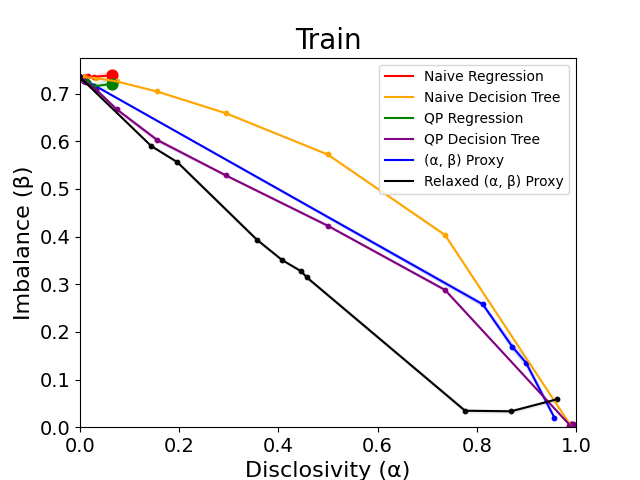
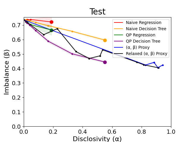
Figure 2: Tradeoff of disclosivity vs. imbalance on the Adult data set w/ race as sensitive feature

Data and Results Summary

We test our method on the Bank Marketing data setMoro et al. (2014); Dua and Graff (2017) and the Adult data set Dua and Graff (2017). The Bank Marketing data set consists of 45211 samples with 48 non-sensitive attributes and a sensitive attribute of job type. The downstream classification goal is to predict whether a client will subscribe a term deposit based on a phone call marketing campaign of a Portuguese banking institution. The Adult data set consists of 48842 samples with 14 non-sensitive attributes, and we select race as the sensitive attribute. The classification task associated with the data set is to determine whether individuals make over $50K dollars per year. We find that in-sample, the Relaxed $(\alpha,\beta)$ proxy consistently Pareto-dominates the others. The QP Decision Tree and $(\alpha,\beta)$ proxy also perform well, with neither consisently Pareto-dominating the other. Out-of-sample, the QP Decision Tree proxy and the Relaxed $(\alpha,\beta)$-proxy tended to perform the best, followed by the $(\alpha,\beta)$ proxy.

5.1 Tradeoff of Disclosivity and Imbalance

We analyze the performance of the six candidate proxies on the Bank Marketing Data set (Figure 1). We observe that both the $(\alpha,\beta)$ proxies and the QP Decision Tree proxy exhibit favorable performance in-sample, driving the imbalance to just above zero at higher disclosivity levels. The plot on the test set shows a more modest improvement in balance as the disclosivity is increased to about $0.4$. We also analyze the test and train performance of the three candidate proxies on the Adult Data set (Figure 2), observing that the Relaxed $(\alpha,\beta)$ proxy Pareto-dominates the remaining proxies in-sample. The QP Regression and Naive Regression proxy both have short tradeoff curves, never reaching a level of imbalance below $0.7$ in the training data and $0.65$ in the testing data. In contrast, the QP Decision Tree and $(\alpha,\beta)$ proxies span the full range of $\alpha$ and achieve $\beta$ values between 0 and 0.7.

5.2 Group Proportions Before and After Filtering

In Figure 3, we visualize the change in balance for three values of $\alpha$ induced by the Relaxed $(\alpha,\beta)$ proxy on the Marketing Data set. The leftmost plot corresponds to a discrepancy budget of zero. As expected, without the flexibility to make any splits, the proxy induces a trivial uniform sampling. With a budget of $0.1$, we observe that the proxy function can be used to filter the data set into a slightly more balanced sub-sample, both in the train set and the test set. Finally, with an $\alpha$ of only 0.2, the proxy produces an almost perfectly balanced data set in-sample.

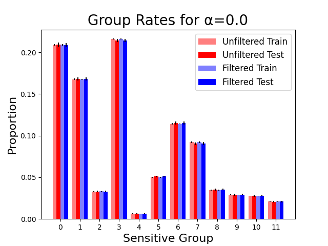
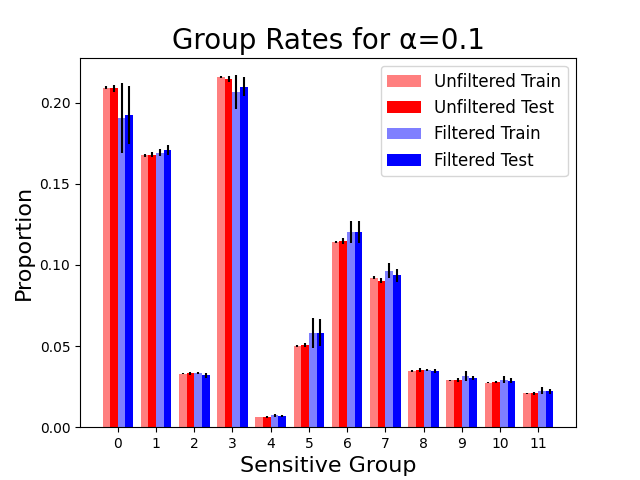
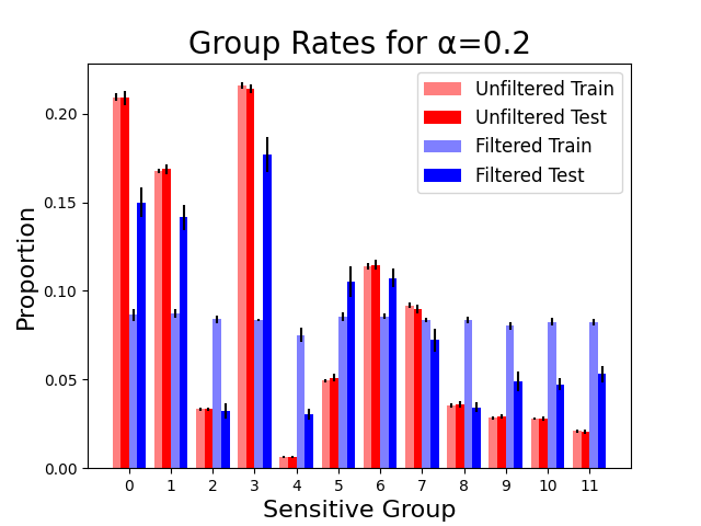
Figure 3: Group proportions on the Bank Marketing data set. It also can be observed that the splitting algorithm begin to take effect where filtered set gets closer to uniform distribution when increasing budget $\alpha$. With only a small budget 0.2, we achieved near-perfect data balance in-sample; on the test split, we also increased the proportion of the originally least represented group to $\sim$4.5 times.

In Figure 4, we display several heat maps for the conditional distribution matrices output by the $(\alpha,\beta)$ proxy on the Adult Data set over three choices of $\alpha$. The number of rows is different for each subplot because each row corresponds to a leaf of our tree, or a proxy group. Each column corresponds to one of the sensitive groups $z$. The colors indicate the conditional distribution of $z$ given the proxy group. The first plot on the left indicates the resulting matrix when the disclosivity budget is 0, which corresponds to the base rates $\Pr_{z\sim D}[z=i]$ because we have not yet split the domain. The middle plot corresponds to a heat map for the proxy with disclosivity of $.82$. Observe that at this stage, we have split the sample space into three proxy groups. However, no conditional distribution deviates from the prior by more than $0.82$ for each element. Finally, on the right, we show the conditional distribution produced with disclosivity of $0.97$. Note that in this plot sensitive attribute $2$ has a posterior probability of 1 in proxy group 1, while its prior probability was only about $0.03$.

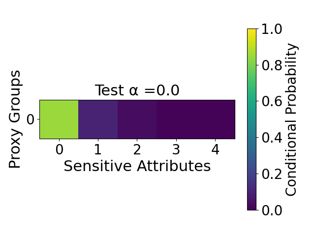
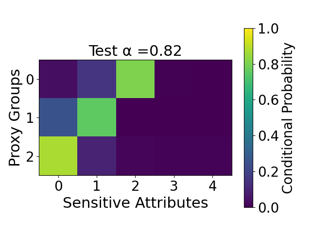
Figure 4: Conditional Distribution Matrices of $z|\hat{z}$ on Adult Data set.

6 Discussion

The experiments show that the $(\alpha,\beta)$, $(\alpha,\beta)$ Relaxed, and QP Decision Tree proxies are empirically effective in improving balance while lowering disclosivity. We emphasize that while the QP proxies (our secondary contribution) are appealingly simple and provide a range of disclosivity levels after post-processing, they have the limitation that they still involve directly training a classifier for the attribute. In contrast, the $(\alpha,\beta)$ proxies (our primary contribution) never involve training a classifier at any step of the process that is more disclosive than a pre-specified threshold. Finally, we remark that our work does not provide guarantees on the downstream fairness effects on models trained using the filtered data. We believe that if our meta-algorithm can be augmented to induce minimal group distortion while filtering, this would have desirable effects not just in terms of the balance of a sample but also in terms of a variety of downstream fairness desiderata for models trained on these data.

Appendix A Appendices

A.1 Additional Experimental Details

Definition 14 (Paired Regression Classifier).

The paired regression classifier operates as follows: We form two weight vectors, $z^{0}$ and $z^{1}$, where $z^{k}_{i}$ corresponds to the penalty assigned to sample $i$ in the event that it is labeled $k$. For the correct labeling of $x_{i}$, the penalty is $0$. For the incorrect labeling, the penalty is the current sample weight of the point, $w_{V}$. We fit two linear regression models $h^{0}$ and $h^{1}$ to predict $z^{0}$ and $z^{1}$, respectively, on all samples. Then, given a new point $x$, we calculate $h^{0}(x)$ and $h^{1}(x)$ and output $h(x)=\operatorname*{argmin}_{k\in\{0,1\}}h^{k}(x)$.

A.1.1 Interpolation Procedure

To interpolate between a uniform and a proxy-specific sampling strategy $\rho$, we first compute $\hat{z}$ with the proxy. Then, with probability $\eta\ in[0,1]$, we re-assign the proxy label to be any of the elements in the range of the proxy with equal probability. Finally, we apply Algorithm 2 to sample according to the post-processed proxy labels. We do this with $\eta=0,0.1,0.2,...,1$ and plot the balance and disclosivity of the corresponding dataset with respect to the post-processed proxy values.

A.1.2 Data Split, Hyperparameter Choices, and Compute Time

For each experiment, we run trials with 20 different seeds, and for each seed, we input a grid of values with increments of 0.05 for the disclosivity parameter, $\alpha$, evenly spaced between $0$ and $1$. We then average over the 20 seeds for each $\alpha$ and calculate empirical $95\%$ confidence intervals. Each dataset is split into two parts, with $\frac{2}{3}$ of the samples going into the training set and $\frac{1}{3}$ going into the test set. On the Adult Dataset, one run over the grid of $\alpha$ values typically took between 20 minutes and two hours for the $(\alpha,\beta)$ proxy and between 10 minutes and 50 minutes for the $(\alpha,\beta)$ Relaxed proxy. On the Marketing Dataset, running one full experiment over the grid of $\alpha$ values took about three hours for both the $(\alpha,\beta)$ proxy and $(\alpha,\beta)$ Relaxed Proxy. The parameter $\gamma$ was set to 0.1, the maximum height of the proxy tree was set to 20, and the learning process was stopped once the distance between the convex hull of the conditional distribution matrix and the uniform distribution fell below 0.1.

A.2 Extension to Intersecting Groups

Our framework can easily be extended to the case where group membership need not be disjoint. We will let the sensitive attribute domain $Z$ be a binary vector of length $K$, such that $z\in\mathcal{Z}=\{0,1\}^{K}$ is a vector of sensitive attributes. We will assume $\mathcal{Z}$ is composed of $G$ group classes $\{g_{i}\}_{i=1}^{G}$ (e.g., sex, race, etc), and each group class $g_{i}$ has $k_{i}$ groups. Thus, the vector $z$ will indicate all possible group memberships, where the length of the vector of group memberships is $K=\sum_{i=1}^{G}k_{i}$.

Definition 15.

We will say that a dataset $D$ is balanced with respect to $K$ intersecting groups if, for any group class $\{g_{i}\}_{i=1}^{G}$ composed of groups $\{g_{i_{j}}\}_{j=1}^{k_{i}}$, $\Pr_{z\sim D}[z[g_{i_{j}}]=1]=\frac{1}{k_{i}}$ for all $j$.

In the remainder of the analysis, we replace $U$ with $U_{\text{intersect}}=(\frac{1}{k_{1}},...,\frac{1}{k_{1}},...,\frac{1}{k_{G}},...,\frac{1}{k_{G}})$.

Definition 16.

We say that a dataset $D$ is $\beta$-approximately balanced with respect to $K$ intersecting groups if

$$\lVert(\Pr_{z\sim D}[z[g_{1_{1}}]=1],\Pr_{z\sim D}[z[g_{1_{2}}]=1],...,\Pr_{z\sim D}[z[g_{G_{k_{G}-1}}]=1],\Pr_{z\sim D}[z[g_{G_{k_{G}}}]=1])-U_{\text{intersect}}\rVert_{2}\leq\beta$$

A.3 Missing Definitions from Section 2

Consider a zero-sum game between two players, a Learner with strategies in $S_{1}$ and an Auditor with strategies in $S_{2}$. The payoff function of the game is $U:S_{1}\times S_{2}\rightarrow\mathbb{R}_{\geq 0}$.

Definition 17 (Approximate Equilibrium).

A pair of strategies
$(s_{1},s_{2})\in S_{1}\times S_{2}$ is said to be a $\nu$-approximate minimax equilibrium of the game if the following conditions hold:

$$U(s_{1},s_{2})-\min_{s^{\prime}_{1}\in S_{1}}U(s^{\prime}_{1},s_{2})\leq\nu,$$

$$\max_{s^{\prime}_{2}\in S_{2}}U(s_{1},s^{\prime}_{2})-U(s_{1},s_{2})\leq\nu$$

Freund and Schapire Freund and Schapire [1996] show that if a sequence of actions for the two players jointly has low regret, then the uniform distribution over each player’s actions forms an approximate equilibrium:

Theorem 4 (No-Regret Dynamics Freund and Schapire [1996]).

Let $S_{1}$ and $S_{2}$ be convex, and suppose $U(\cdot,s_{2}):S_{1}\to\mathbb{R}_{\geq 0}$ is convex for all $s_{2}\in S_{2}$ and $U(s_{1},\cdot):S_{2}\to\mathbb{R}_{\geq 0}$ is concave for all $s_{1}\in S_{1}$. Let $(s_{1}^{1},s_{1}^{2},\ldots,s_{1}^{T})$ and $(s_{2}^{1},s_{2}^{2},\ldots,s_{2}^{T})$ be sequences of actions for each player. If for $\nu_{1},\nu_{2}\geq 0$, the regret of the players jointly satisfies

$$\sum_{t=1}^{T}U(s_{1}^{t},s_{2}^{t})-\min_{s_{1}\in S_{1}}\sum_{t=1}^{T}U(s_{1},s_{2}^{t})\leq\nu_{1}T$$

$$\max_{s_{2}\in S_{2}}\sum_{t=1}^{T}U(s_{1}^{t},s_{2})-\sum_{t=1}^{T}U(s_{1}^{t},s_{2}^{t})\leq\nu_{2}T$$

then the pair $(\bar{s}_{1},\bar{s}_{2})$ is a $(\nu_{1}+\nu_{2})$-approximate equilibrium, where $\bar{s}_{1}=\frac{1}{T}\sum_{t=1}^{T}s_{1}^{t}\in S_{1}$ and $\bar{s}_{2}=\frac{1}{T}\sum_{t=1}^{T}s_{2}^{t}\in S_{2}$ are the uniform distributions over the action sequences.

Theorem 5 (Hoeffding Bound).

Let $X_{1},...,X_{m}$ be independent random variables such that $a_{i}\leq X_{i}\leq b_{i}$ almost surely. Consider the sum of these random variables, $S_{m}=X_{1}+...X_{m}$. Then, for all $t\geq 0$,

$$Pr\left[|S_{m}-E\left[S_{m}\right]\rvert\geq t\right]\leq\exp{\frac{-2t^{2}}{\sum_{i=1}^{m}(b_{i}-a_{i})^{2}}}$$

Online Projected Gradient Descent

Online Projected Gradient Descent is a no-regret online learning algorithm we can formulate as a two-player game over $T$ rounds. At each round $t\leq T$, a Learner selects an action $\theta^{t}$ from its action space $\Theta\subset\mathbb{R}^{d}$ (equipped with the $L_{2}$ norm), and an Auditor responds with a loss function $\ell^{t}:\Theta\to\mathbb{R}_{\geq 0}$. The learner’s loss at round $t$ is $\ell^{t}(\theta^{t})$. If the learner is using an algorithm $A$ to select its action each round, then the learner wants to pick $A$ so that the regret $R_{A}(T):=\sum_{t=1}^{T}\ell^{t}(\theta^{t})-\min_{\theta\in\Theta}\sum_{i=1}^{T}\ell^{t}(\theta)$ grows sublinearly in $T$. When $\Theta$ and the loss function played by the Auditor are convex, the Learner may deploy Online Projected Gradient Descent (Algorithm (5)) to which the Auditor best responds. In this scenario, in each round $t$, the Learner selects $\theta^{t+1}$ by taking a step in the opposite direction of the gradient of that round’s loss function, and $\theta^{t+1}$ is projected into the feasible action space $\Theta$. Pseudocode and the regret bound are included below.

Input: learning rate $\eta$

Initialize the learner $\theta^{1}\in\Theta$;

for $t=1,2,\ldots$ do

       Learner plays action $\theta^{t}$;

       Adversary plays loss function $\ell^{t}$;

       Learner incurs loss of $\ell^{t}(\theta^{t})$;

       Learner updates its action: $\theta^{t+1}=\text{Proj}_{\Theta}\left(\theta^{t}-\eta\nabla\ell^{t}(\theta^{t})\right)$;

      

end for

Algorithm 5 Online Projected Gradient Descent

Theorem 6 (Regret for Online Projected Gradient Descent Zinkevich [2003]).

Suppose $\Theta\subseteq\mathbb{R}^{d}$ is convex, compact and has bounded diameter $D$: $\sup_{\theta,\theta^{\prime}\in\Theta}\left\|\theta-\theta^{\prime}\right\|_{2}\leq D$. Suppose for all $t$, the loss functions $\ell^{t}$ are convex and that there exists some $G$ such that $\left\|\nabla\ell^{t}(\cdot)\right\|_{2}\leq G$. Let $\mathcal{A}$ be Algorithm 5 run with learning rate $\eta=D/(G\sqrt{T})$. We have that for every sequence of loss functions $(\ell^{1},\ell^{2},\ldots,\ell^{T})$ played by the adversary, $R_{\mathcal{A}}(T)\leq GD\sqrt{T}$.

A.4 Missing Derivation from Section 4.2

We now present a subroutine that our algorithm will use to find an $\alpha$-proxy. To do this, we use the left-hand side of Equation (2) as our objective and the non-disclosive desiderata from Section 2 as our constraints. For ease of notation, we will let $r_{k}=\Pr_{z\sim D}[z=k]$

|s| h_V∈H∑_j=1^m_V w_V(x_j) h_V(x_j) ( - Q_V,U’,γ + ∑_k=1^K 1_z_j = k⋅(U_k’ - U_k) ) ∑j=1mVwV(xj) hV(xj) 1zj= k∑VwV(xj)hV(xj) - r_k≤α  ∀k ∑j=1mVwV(xj)(1-hV(xj)) 1zj= k∑j=1mVwV(xj)(1-hV(xj))- r_k ≤α  ∀k r_k - ∑j=1mVwV(xj)hV(xj) 1zj= k∑VwV(xj)hV(xj)≤α  ∀k r_k - ∑j=1mVwV(xj)(1- hV(xj)) 1zj= k∑j=1mVwV(xj)(1-hV(xj)) ≤α  ∀k

Next, we will appeal to strong duality to derive the corresponding Lagrangian. We note that computing an approximately optimal solution to the linear program corresponds to finding approximate equilibrium strategies for both players in the game in which one player, “The Learner,” controls the primal variables and aims to minimize the Lagrangian value. The other player, “The Auditor,” controls the dual variables and seeks to maximize the Lagrangian value. If we construct our algorithm in such a way that it simulates repeated play of the Lagrangian game such that both players have sufficiently small regret, we can apply Theorem 4 to conclude that our empirical play converges to an approximate equilibrium of the game. Furthermore, our algorithm will be oracle efficient: it will make polynomially many calls to oracles that solve weighted cost-sensitive classification problems over $\mathcal{H}$. We define a weighted cost-sensitive classification oracle as follows:

Definition 18 (Weighted Cost-Sensitive Classification Oracle for $\mathcal{H}$).

An instance of a Cost-Sensitive Classification problem, or a $CSC$ problem, for the class $\mathcal{H}$, is given by a set of $n$ tuples $\{w_{V}(x_{j}),x_{j},c_{i}^{0},c_{i}^{1}\}_{i=1}^{n}$ such that $c_{i}^{1}$ corresponds to the cost for predicting label 1 on sample $x_{j}$ and $c_{i}^{0}$ corresponds to the cost for prediction label $0$ on sample $x_{j}$. The weight of $x_{j}$ is denoted by $w(x_{j})$. Given such an instance as input, a $CSC(\mathcal{H})$ oracle finds a hypothesis $h\in\mathcal{H}$ that minimizes the total cost across all points: $h\in\operatorname*{argmin}_{h^{\prime}\in\mathcal{H}}\sum_{j=1}^{n}w(xj)\left[h^{\prime}(x_{j})c_{i}^{1}+(1-h^{\prime}(x_{j}))c_{i}^{0}\right]$.

To turn Program (A.4) form amenable to our two-player zero-sum game formulation, we expand $\mathcal{H}$ to $\Delta\mathcal{H}$, allow our splitting function to be randomized, and take expectations over the objective and constraints with respect to $\tilde{h}$. Doing so yields the following CSC problem to be solved for vertex $V$:

|s| ~h_V∈ΔHE_~h_V ∼ΔH∑_j=1^m_V w_V(x_j)~h_V(x_j) ( - Q_V,U’,γ + ∑_k=1^K 1_z_j = k (U_k’ - U_k)

References

- Agarwal et al. [2018] Alekh Agarwal, Alina Beygelzimer, Miroslav Dudík, John Langford, and Hanna M. Wallach. A reductions approach to fair classification. CoRR, abs/1803.02453, 2018. URL http://arxiv.org/abs/1803.02453.
- Batista et al. [2003] Gustavo E. A. P. A. Batista, Ana Lúcia Cetertich Bazzan, and Maria Carolina Monard. Balancing training data for automated annotation of keywords: a case study. In WOB, 2003.
- Batista et al. [2004] Gustavo E. A. P. A. Batista, Ronaldo C. Prati, and Maria Carolina Monard. A study of the behavior of several methods for balancing machine learning training data. SIGKDD Explor. Newsl., 6(1):20–29, jun 2004. ISSN 1931-0145. doi: 10.1145/1007730.1007735. URL https://doi.org/10.1145/1007730.1007735.
- Chawla et al. [2002] Nitesh V. Chawla, Kevin W. Bowyer, Lawrence O. Hall, and W. Philip Kegelmeyer. Smote: Synthetic minority over-sampling technique. J. Artif. Int. Res., 16(1):321–357, June 2002. ISSN 1076-9757.
- Diana et al. [2022] Emily Diana, Wesley Gill, Michael Kearns, Krishnaram Kenthapadi, Aaron Roth, and Saeed Sharifi-Malvajerdi. Multiaccurate proxies for downstream fairness. In 2022 ACM Conference on Fairness, Accountability, and Transparency, FAccT ’22, page 1207–1239, New York, NY, USA, 2022. Association for Computing Machinery. ISBN 9781450393522. doi: 10.1145/3531146.3533180. URL https://doi.org/10.1145/3531146.3533180.
- Douzas et al. [2018] Georgios Douzas, Fernando Bacao, and Felix Last. Improving imbalanced learning through a heuristic oversampling method based on k-means and SMOTE. Information Sciences, 465:1–20, oct 2018. doi: 10.1016/j.ins.2018.06.056. URL https://doi.org/10.1016%2Fj.ins.2018.06.056.
- Dua and Graff [2017] Dheeru Dua and Casey Graff. UCI machine learning repository, 2017. URL http://archive.ics.uci.edu/ml.
- Dwork and Roth [2014] Cynthia Dwork and Aaron Roth. The algorithmic foundations of differential privacy. Found. Trends Theor. Comput. Sci., 9(3–4):211–407, aug 2014. ISSN 1551-305X. doi: 10.1561/0400000042. URL https://doi.org/10.1561/0400000042.
- Dwork et al. [2006] Cynthia Dwork, Frank McSherry, Kobbi Nissim, and Adam Smith. Calibrating noise to sensitivity in private data analysis. In Theory of Cryptography: Third Theory of Cryptography Conference, TCC 2006, New York, NY, USA, March 4-7, 2006. Proceedings 3, pages 265–284. Springer, 2006.
- Elliott et al. [2009] Marc N. Elliott, Peter A. Morrison, Allen M. Fremont, Daniel F. McCaffrey, Philip M Pantoja, and Nicole Lurie. Using the census bureau’s surname list to improve estimates of race/ethnicity and associated disparities. Health Services and Outcomes Research Methodology, 9:69–83, 2009.
- Freund and Schapire [1996] Yoav Freund and Robert E. Schapire. Game theory, on-line prediction and boosting. In Proceedings of the Ninth Annual Conference on Computational Learning Theory, 1996.
- Han et al. [2005] Hui Han, Wenyuan Wang, and Binghuan Mao. Borderline-smote: A new over-sampling method in imbalanced data sets learning. In International Conference on Intelligent Computing, 2005.
- Hardt et al. [2016] Moritz Hardt, Eric Price, and Nati Srebro. Equality of opportunity in supervised learning. In D. Lee, M. Sugiyama, U. Luxburg, I. Guyon, and R. Garnett, editors, Advances in Neural Information Processing Systems, volume 29. Curran Associates, Inc., 2016. URL https://proceedings.neurips.cc/paper_files/paper/2016/file/9d2682367c3935defcb1f9e247a97c0d-Paper.pdf.
- Hart [1968] Peter E. Hart. The condensed nearest neighbor rule. IEEE Transactions on Information Theory, pages 515–516, 1968.
- He et al. [2008] Haibo He, Yang Bai, Edwardo A. Garcia, and Shutao Li. Adasyn: Adaptive synthetic sampling approach for imbalanced learning. 2008 IEEE International Joint Conference on Neural Networks (IEEE World Congress on Computational Intelligence), pages 1322–1328, 2008.
- Jagielski et al. [2018] Matthew Jagielski, Michael J. Kearns, Jieming Mao, Alina Oprea, Aaron Roth, Saeed Sharifi-Malvajerdi, and Jonathan R. Ullman. Differentially private fair learning. CoRR, abs/1812.02696, 2018. URL http://arxiv.org/abs/1812.02696.
- Mani and Zhang [2003] Inderjeet Mani and Jianping Zhang. knn approach to unbalanced data distributions: A case study involving information extraction. Workshop on Learning from Imbalanced Datasets II, ICML, 126:1–7, 2003.
- Mccaffrey et al. [2005] Daniel Mccaffrey, Greg Ridgeway, and Andrew Morral. Propensity score estimation with boosted regression for evaluating causal effects in observational studies. Psychological methods, 9:403–25, 01 2005. doi: 10.1037/1082-989X.9.4.403.
- Menardi and Torelli [2012] Giovanna Menardi and Nicola Torelli. Training and assessing classification rules with imbalanced data. Data Mining and Knowledge Discovery, 28:92–122, 2012.
- Moro et al. [2014] Sérgio Moro, Paulo Cortez, and Paulo Rita. A data-driven approach to predict the success of bank telemarketing. Decision Support Systems, 62:22–31, 2014. ISSN 0167-9236. doi: https://doi.org/10.1016/j.dss.2014.03.001. URL https://www.sciencedirect.com/science/article/pii/S016792361400061X.
- Nguyen et al. [2009] Hien M. Nguyen, Eric W. Cooper, and Katsuari Kamei. Borderline over-sampling for imbalanced data classification. Int. J. Knowl. Eng. Soft Data Paradigms, 3:4–21, 2009.
- Tomek [1976a] I. Tomek. An experiment with the edited nearest-neighbor rule. IEEE Transactions on Systems, Man, and Cybernetics, SMC-6(6):448–452, 1976a. doi: 10.1109/TSMC.1976.4309523.
- Tomek [1976b] I. Tomek. Two modifications of cnn. IEEE Transactions on Systems, Man, and Cybernetics, 6:769–772, 1976b.
- U.S. [2023] U.S. Students for fair admissions, inc. v. president and fellows of harvard college, 2023.
- Voicu [2016] Ioan Voicu. Using first name information to improve race and ethnicity classification. Statistics and Public Policy, 5:1 – 13, 2016.
- Wilson [1972] Dennis L. Wilson. Asymptotic properties of nearest neighbor rules using edited data. IEEE Trans. Syst. Man Cybern., 2:408–421, 1972.
- Zhang et al. [2018] Hongyi Zhang, Moustapha Cisse, Yann N. Dauphin, and David Lopez-Paz. mixup: Beyond empirical risk minimization, 2018.
- Zhang [2016] Yan Zhang. Assessing fair lending risks using race/ethnicity proxies. Comparative Political Economy: Regulation eJournal, 2016.
- Zinkevich [2003] Martin Zinkevich. Online convex programming and generalized infinitesimal gradient ascent. In Proceedings of the Twentieth International Conference on Machine Learning. Washington, DC, 2003.