Scaling and Resizing Symmetry in Feedforward Networks
1 Introduction
Deep learning achievements during the last decade are quite impressive in fields such as pattern recognition [1], speech recognition [2], large language models [3, 4], video and board games [5, 6] and neurobiology [7, 8], just to mention a few. This success has come with increasingly larger networks size, deep and complexity [9, 10], which often lead to undesired effects such a exploding or vanishing gradients [11] which hinders the minimization of the cost function.
Early work in deep learning [11, 12] has shown that exploding or vanishing gradients crucially depend on weights initialization, and henceforth a properly chosen random distribution of weights at initialization can prevent such exploding or vanishing gradients.
The dependence of correlations on the deep of untrained random initialized feedforward networks has been studied in [13, 14, 15], where it has been found that random Gaussian initialization develops an order/chaos phase transition in the space of weights-biases variances, which in turn translates into the development of vanishing/exploding gradients. Even more interestingly, the existence of a critical line separating the ordered from the chaotic phase, acts as a region where information can be propagated over very deep scales, and as such, signals the ability to train extremely deep networks at criticality. This phase transition has been observed so far also in convolutional networks [16], autoencoders [17] and recurrent networks [18].
In this paper, we build on the results of [14, 15], by looking a bit closer into the phase transition properties. After a quick review of the relevant results from [14, 15], we offer an analogous view for the covariance matrix propagation through a feedforward network in terms of a two-dimensional statistical physical system. Based on such analogy, we propose an order parameter associated to the phase transition and show that a scaling symmetry in deepness arise at the critical phase, for which we compute numerically some critical exponents. Then we argue at the level of conjecture, that such scaling symmetry translates into a re-sizing symmetry for other dimension of the feedforward network, such as input data size, hidden layers width and stochastic gradient descent batch size. Lately, we perform experiments showing that resizing down by a half the input data, hidden layers width or stochastic gradient descent batch size has little detrimental impact on learning performance at the critical phase.
This results suggest that random initialization of feedforward networks at the critical phase, might allow to train networks with much less data or smaller architectures, leading consequently to speed up learning.
2 Theoretical Background
In this section we present few very well known definitions and properties of feedforward deep neural networks and set some notation.
2.1 Feedforward Networks
Let us start by considering a fully-connected untrained deep feedforward neural network with layers, each of width , with denoting the corresponding layer label. Let be the matrix of weights linking the layer to the layer (hence of dimension ) and the bias vector at layer . The vector output at each layer (or post-activation) is then defined by the recursion relation:
| (2.1) |
with the initial condition input-data, of dimension . The activation function is a scalar function acting element-wise on the vector components of its argument. For now we consider to have a sigmoid shape
| (2.2) |
but otherwise to be arbitrary 111However, for the experiments later in this note we will use .
The goal of the network is to learn the mapping,
| (2.3) |
that both, best approximate the input data to the output data, and that best generalizes to new data. This is done by minimizing a cost function measuring how far off the learned mapping is from the actual input-output map. Such cost function is in most cases taken to be the sum of square errors:
| (2.4) |
An important object characterizing is the input-output Jacobian given by:
| (2.5) |
with the components of given by .
We want to consider an initial value for the weights and biases to be drawn from the following normal distributions: , . The weight re-scaling over is to preserve the weights finite for large sizes of hidden layers.
2.2 Mean Field Theory of Deep Feedforward Signal Propagation
2.3 Physical Statistical System
We want to understand how the empirical distribution of pre-activations propagates through the network. To do that, we can define the following partition function,
| (2.6) |
with a quadratic Hamiltonian given by,
| (2.7) |
with an arbitrary parameter and being the covariance matrix,
| (2.8) |
We additionally define the free energy as it’s usual in physical statistical systems,
| (2.9) |
from which we can see the following relation
| (2.10) |
As we will see in next subsection, as propagates through the network, after few layers it will eventually reach an equilibrium constant value , i,e,
| (2.11) |
For convenience, let us split the Hamiltonian in diagonal and non-diagonal parts,
| (2.12) |
with
| (2.13) |
For large , it has been shown in [14, 15] that converge to a zero mean Gaussian distribution over the given layer , and in such limit, we can replace the sums for integrals with the corresponding Gaussian probability density (see [14] for details). At equilibrium, we can write the diagonal Hamiltonian as,
| (2.14) |
whereas the non-diagonal looks like,
| (2.15) |
with,
| (2.16) |
here and are independent standard Gaussian variables, while and are correlated Gaussian variables with covariance matrix , which become at equilibrium.
Once the system reach equilibrium, we approximate the partition function by,
| (2.17) |
where is the total number of layers. From it, we have
| (2.18) |
which lead us to the following consistency equation,
| (2.19) |
with a similar equation for the non-diagonal,
| (2.20) |
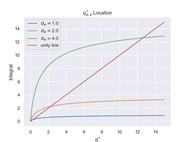
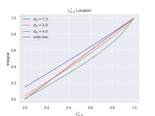
The solutions to these consistency conditions, or fixed points, correspond to the equilibrium values of the covariance matrix. They can be solved very efficiently numerically, by pinning down the interception of the unity line with the value from the integrals at the right hand side of both conditions, as illustrated at the left frames of figures 1 and 2,
2.4 Dynamical System
Although the storytelling in subsection above might be useful to build some physical intuition, it does not provides us with a good view of the non-equilibrium dynamics that the system undergoes. For that it will convenient to resort back to [14, 15], where instead of focusing solely on the equilibrium state, the random network has been approached from the point of view of dynamical systems, by considering the recursion relations leading to (2.19) and (2.20),
| (2.21) |
| (2.22) |
with,
| (2.23) |
for the diagonal and non-diagonal components respectively. This recursions define an iterative map.
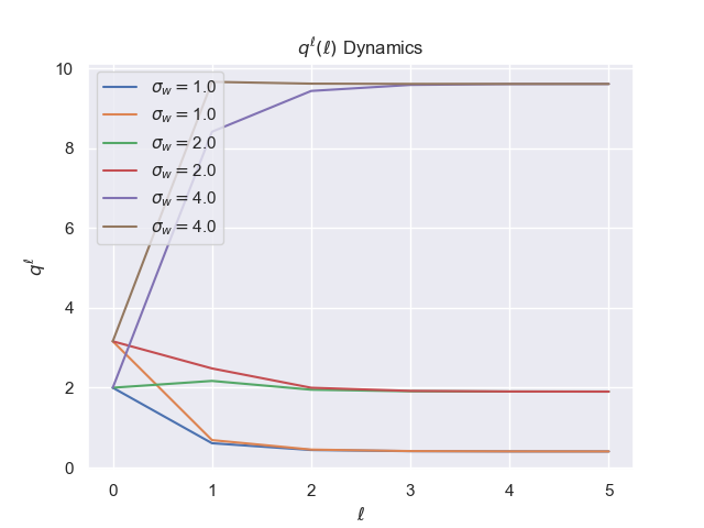
By iterating this recursion a few times, we can see the dynamics of the covariance matrix before reaching equilibrium, as shown at the right frame in figure 1. Notice that the fixed point is reached after few layers.
For the non-diagonal component, it is convenient to use the normalized correlation coefficient , to write instead,
| (2.24) |
with
| (2.25) |
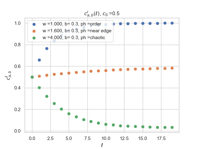
exhibit a more interesting behavior: for low values of it only has one fixed point at which is also stable, but for values larger than a given ( for the cases depicted in figure 2), the recursion develops a second fixed stable point, as shown in the left figure 2, and the fixed point becomes unstable, signaling a phase transition in space. For a given tuple of values , we can check the stability of the covariance map by looking into the derivative of the iterative map at the fixed point,
| (2.26) |
so the critical values are those that solve the equation .
From the right figure 2, we can see that it takes longer for the fixed point to be reached than it takes to reach . In figure 2 we have used in all cases, in which case the critical turns out to be . For values below the network correlates initial data, for values above the network uncorrelates initial data, and for values near the network tend to preserve the initial data correlations. A property of a dynamical system signaling chaotic behavior is that by evolving two infinitesimally close initial conditions, they both reach values significatively apart from each other. Considering the covariance matrix, by initializing a network with random Gaussian weights at , and tracking two input data points initially very correlated (very close in correlation space), they will get uncorrelated as they propagate through the network (separate from each other in correlation space), signaling a chaotic phase. Conversely, uncorrelated initial data points, will correlated for an initialization with , signaling an ordered phase. This two phases are related to exploding or vanishing gradients during stochastic gradient descent.
In the next section, we would like to take a closer look into the phase.
3 Phase Transition
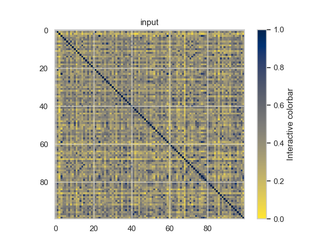
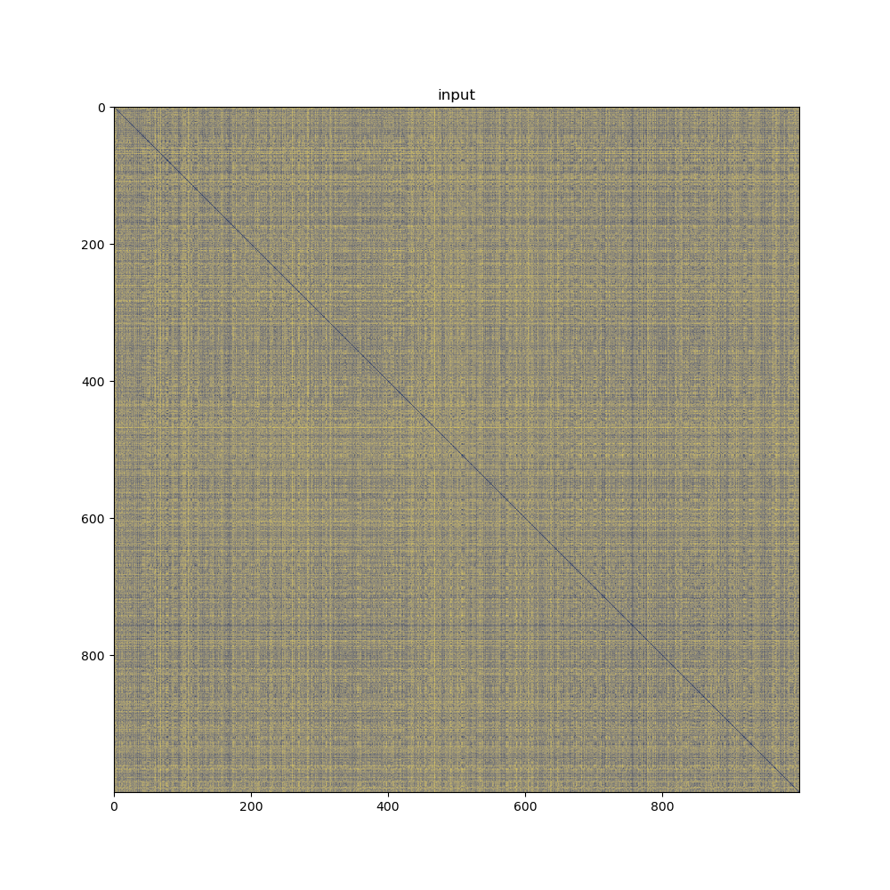
For the examples and experiments treated in the rest of this note, we will take the MNIST dataset [19, 20] of handwritten numbers. Let us then consider the normalized correlation coefficient matrix, or covariance matrix of such input data (depicted in figure 3 for a subset of 100 input data points for visualization clarity) as it propagates through the network. Think of this matrix as a two-dimensional lattice statistical mechanical system at some initial state (out of equilibrium), where each “pixel” or component of the matrix represents a physical quantity ( such a magnetic moment, for example) whose value is between zero and one. Now consider that the system evolution is the same as the one undergone by the covariance matrix as it propagates through a feedforward network. A given initial can be thought of as an external field (such a magnetic or electric field), and a given as a temperature.
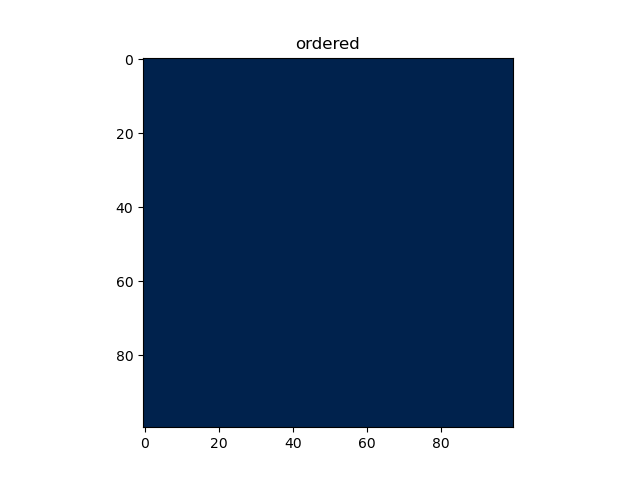
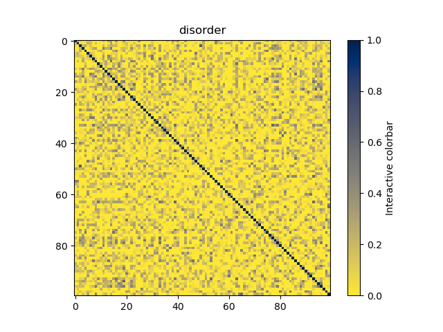
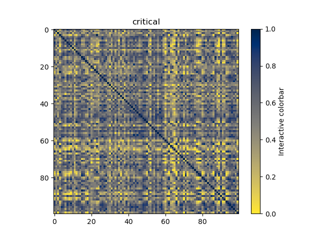
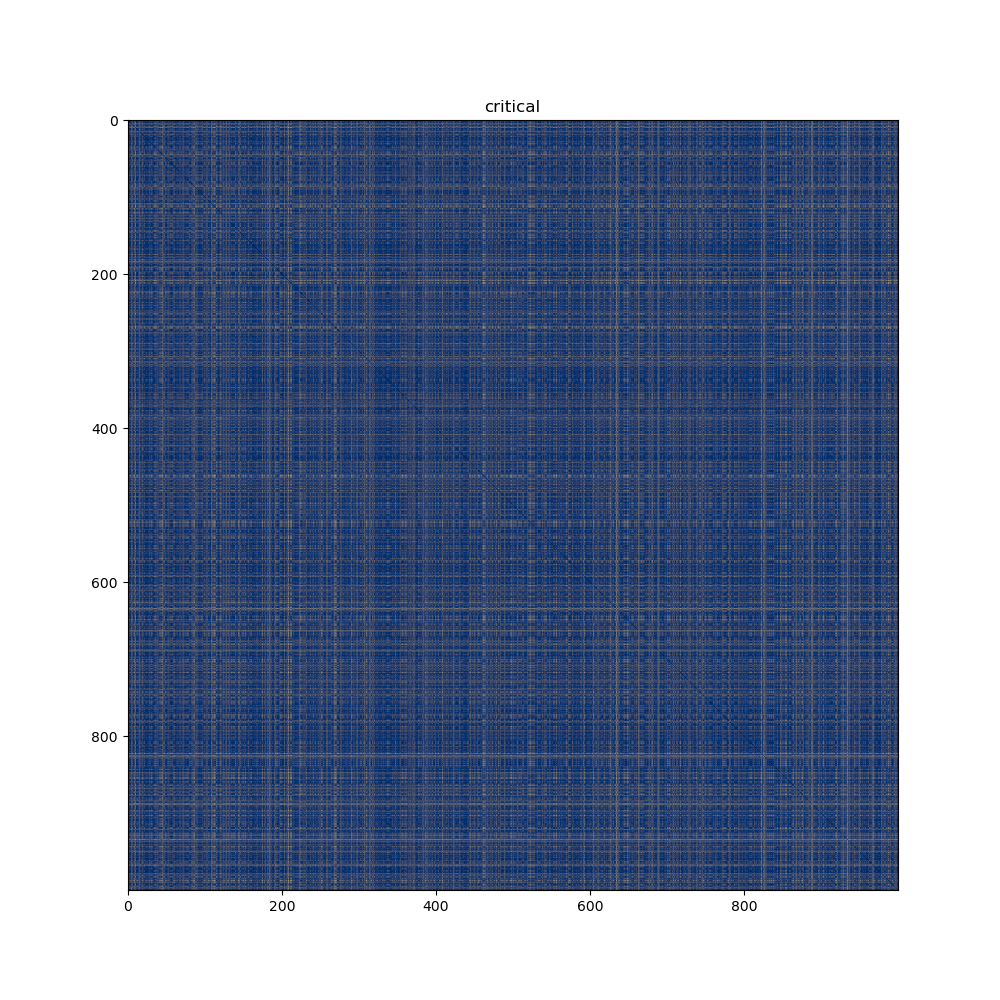
Now imagine that we set a “temperature” and a “magnetic field” , and let the system evolve towards equilibrium 222 and are only pictorial analogies of an actual temperature and external field, in particular they do not even have the proper units.. Evolving in this context means that we let the initial data propagate through the network with the given random initialization. Once the data propagate across all layers in the order phase, the covariance matrix looks like a system at zero temperature (completely correlated), the order phase looks like a system at infinite temperature (completely uncorrelated) after propagation in the chaotic phase and a system at critical temperature after propagating in the critical phase. To illustrate this, we created a feedforward network with 10 hidden layers, each layer composed of 50 units 333the output layer in this case, is not the one corresponding to the classification problem (ten digits layer), but an arbitrary 50 units layer. and propagate the MNIST data once over initializations corresponding to each of these three phases, then we compute the correlation matrix of the resulting output. The results are illustrated in the pictures at figure 4
By propagating the input data at the ordered phase, the network do a very good job correlating the data whereas at the disorder phase the data gets almost completely uncorrelated. At the critical phase however, even though the network tends to correlated data slightly, it reach a fixed point where the data propagate to a “fix” intermediate (non-saturated) correlation. Within the analogy to statistical physics, we define the following order parameter
| (3.1) |
which we will call, the mean correlation. Here is the number of data points in a given case. In the order phase, is close to one, and we have a large mean correlation, at the disorder phase the is small and we have a vanishing mean correlation. Lastly, at the critical phase, the mean correlation is in between the two other phases. Henceforth, the change of from non-zero to zero signal a phase transition, and that is why we have interpreted it as an order parameter.
Computing the mean correlation for the particular examples displayed in figures 3 and 4 we get the values in table 1.
| Input | Ordered | Disordered | Critical | |
| 0.414 | 0.99 | 0.041 | 0.50 |
This values reflect the values of the corresponding fixed points.
An observation from the table above that will play a role in the next section’s discussion, is that the value of order parameter for the input data is not too far from the value at the critical phase output.
4 Scaling Symmetry
It is well known that physical systems having second order phase transition exhibit scaling symmetry at the critical phase. In this section, we ask the question if such symmetry is also exhibited in the feedforward initializing network that we have discussed in the previous section.
4.1 Theoretical Considerations
One can ask how far the input data need to propagate in order for the correlation matrix to reach its fix point. This question was detailed answered in [15]. For enough large , the covariance matrix approach the fix point exponentially,
| (4.1) |
with indicating that the propagation length is different for the diagonal terms than for the non-diagonals , respectively,
| (4.2) |
and
| (4.3) |
establish a depth scale that measures how far deep the input information propagates into a random initialized network.
We are concerned about the correlation length at the fixed point, therefore evaluating at , reduces it to
| (4.4) |
Since the phase transition occurs when , the correlation length diverges there, hence at the critical phase the information will propagate at all deep lengths, as long as the fixed point has been already reached. This is indeed a signal of scaling symmetry.
In experiments on physical systems as well as in solvable theories, it has been observed that at the critical phase, when the correlation length diverges, the behavior of the covariance (or two-point correlation function) given by (4.1), breaks down, and instead approaches the fixed point in a power-law fashion,
| (4.5) |
with some coefficient, which in the physical literature corresponds to the so-called critical exponents. For the current case of the feedforward network, the break down of (4.1) near the phase transition can be seen by realizing that its derivation at [15] relies on a perturbative expansion around with perturbation parameter given by
| (4.6) |
which becomes of order one around the critical phase, hence breaking the perturbative approximation.
We now want to check experimentally, if such power-law behavior from physical statistical systems, is also observed in the random network phase transition discussed here.
4.2 Critical Exponents for Information Propagation
First we want to check that the power law behavior observed at criticality in phase transitions of physical systems can be, at least approximately, observed in the information propagation in random networks at the critical phase. In order to see that, we have plotted for with an initial input very close to the critical value and fitted to each case a power law of the form,
| (4.7) |
the resulting plots and fits are shown in figure 5, from where
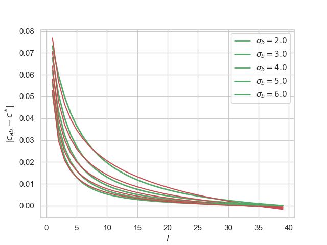
we can see that indeed a power law behavior 4.7 provides a good approximation for the behavior of information propagation very close to criticality. The correspondent fitted critical exponents for each are shown in the table below,
| 2 | 3 | 4 | 5 | 6 | |
|---|---|---|---|---|---|
| 0.213 | 0.406 | 0.545 | 0.653 | 0.743 |
4.3 Exploring Scaling Symmetry in Covariance Space
The divergence of the correlation length in layer space discussed above, provide us with evidence for a scaling symmetry taking place at criticality. This scaling symmetry tell us that, once the critical fixed point is reached, the correlation matrix is preserved through the subsequent layers.
We have observed in table 1 that the input mean correlation for MNIST data set is not too far from the output mean correlation at criticality, which is a consequence of the approximate scaling symmetry in deepness space. We expect such scaling symmetry to be reflected in the output correlation matrix, or in other words: since input mean correlations are approximately preserved for propagation at the critical phase, we should be able to re-size the input correlation matrix in a way that the input mean correlation is approximately preserved in the output mean correlation, and our conjecture is that such mean correlation symmetry is reflected as a symmetry of learning performance at criticality. More concretely, due to the law of large numbers, mean correlations of sub-correlation matrices approximate the mean correlation of the whole matrix. We then can take a subsample of the input data, preserving the input mean correlation. Since such mean correlation is approximately preserved through the network at criticality, the mean correlation of the output correlation matrix does not change appreciably and as a consequence the learning map should not change much and therefore, resizing the input data will preserve (approximately) learning performance, as we will explore experimentally in what follows. For that, we compute the normalized correlation matrix and the mean correlation for the input MNIST data set and propagate the data through the network, in order to compute the matrix correlation and mean correlation of the propagated output. Next, we reduce the size of the input data and compute once again mean correlations for input and output. The graphical representation of input and output correlation matrices is shown in figure 6 for 1000 MNIST examples
The corresponding mean correlation for the input and correlation matrices are shown in table 2 where we can check the conservation of output mean correlations from input resizing.
| Input | Half-Input | Critical Output | Half-Input Critical Output | |
| 0.40 | 0.39 | 0.72 | 0.72 |
Table 2 shows that propagating half the input data has barely any effect on the mean correlation of the output. In next section we will explore the impact of this data resizing on training.
5 Experiments
5.1 Reducing Input Data
Based on last section’s discussion, we can intuitively think that at critical initialization, we can reduce the amount of input data without considerably degrading accuracy in the learned input-output map. In this section we will provide experimental evidence that is the case.
We train a very simple feedforward network on the MNIST data set. Our network consist of 6 hidden layers 444More than two feedforward layers to learn the classification problem of MNIST is a bit overkill, but here we are interested in the impact of many layers. and a 10 units output layer representing the output probabilities for the digits from 0 to 9 555In this section we add a 10-units output layer corresponding to the 10 digits of the MNIST dataset.. We use stochastic gradient descent on a cross-entropy cost function. Since we are only worry for the performance of the network as a function of initial data size, we will not use any particular regularization.
First we train the network with 50000 MNIST examples, and let it run for just some few epochs, getting the accuracies over validation (unseen) data in the three phases as plotted in figure 7 left.


Then we re-train the same architecture but with half the examples, i.e 25000, and from the right figure 7 we can observe that, even though the accuracy and learning speed at the order phase deteriorates considerably (the chaotic case is already very deteriorated even with the full dataset), the performance of the network at the critical phase does not diminish at all, with the advantage that with that many less examples, the network takes almost half the time in running the same number of epochs.
Just out of curiosity, we push harder, and re-train the network with only 15000 examples, and even thought the accuracy at the critical initialization suffer some deterioration, is not as strong as in the chaotic and order phases where the accuracy and learning speed do get very badly behaved. For some practical cases, the small punishment on the accuracy of the learned map at the critical phase maybe beneficial in terms of the smaller number of required input data examples and decreased training time, which in our experiments is three times smaller than when in use of the full data set.

5.2 Reducing Hidden Width and Batch Size
Similarly as to the intuition that resizing of the input data is an approximate symmetry of the output correlation matrix at criticality, we can consider the effect of resizing the width of the hidden layers, in this section we take the same architecture as in the previous subsection but will resize the hidden layers by half, however preserving the same size of the input data.
As in previous section, reducing the hidden width, has almost not detrimental impact on the performance of the network initialized at the critical phase, while it does hurt considerably the performance at initializations in the order and disorder phases, as shown in figure 9.

Lastly, we can also examine the impact of resizing the batch for stochastic gradient descent, while keeping the original sizes for the input data and hidden layers width. We reduce the size of this batch by a half and plot the resulting accuracies over the validation set in figure 10, once again observing little impact performance on initialization at the critical phase, unlike the other two phases.

6 Discussion and Conclusions
In this paper we have studied the phase transition occurring in the propagation of the covariance matrix through a random deep feedforward network. In summary, we have shown that a naive statistical physics description for such system can be developed, which in turns lead us to consider some well known properties of physical phase transitions, such as scaling symmetry at criticality. We additionally argued, that the given scaling symmetry translates into a data-resizing symmetry which in principle, would allow to scale down a large network into a smaller one without degrading learning performance.
It is worth mentioning that more precise correspondences between neural networks and statistical physical system have been developed previously in several other works. Such as those recently developed at [21] and [22]. It would be very interesting to studied the phase transition treated in this note, from the point of view of such interesting physical approaches.
Another recent interesting relation between physical phase transition and deep neural networks have been studied in the context of the loss landscape in [23, 24, 25]. It would be interesting to ask if the phase transitions in random networks studied in this paper has any relation to those studied there.
References
- [1] Alex Krizhevsky, Ilya Sutskever, and Geoffrey E Hinton. Imagenet classification with deep convolutional neural networks. In F. Pereira, C.J. Burges, L. Bottou, and K.Q. Weinberger, editors, Advances in Neural Information Processing Systems, volume 25. Curran Associates, Inc., 2012.
- [2] Awni Hannun, Carl Case, Jared Casper, Bryan Catanzaro, Greg Diamos, Erich Elsen, Ryan Prenger, Sanjeev Satheesh, Shubho Sengupta, Adam Coates, and Andrew Y. Ng. Deep speech: Scaling up end-to-end speech recognition, 2014.
- [3] Alec Radford, Jeffrey Wu, Rewon Child, David Luan, Dario Amodei, Ilya Sutskever, et al. Language models are unsupervised multitask learners. OpenAI blog, 1(8):9, 2019.
- [4] Tom B. Brown, Benjamin Mann, Nick Ryder, Melanie Subbiah, Jared Kaplan, Prafulla Dhariwal, Arvind Neelakantan, Pranav Shyam, Girish Sastry, Amanda Askell, Sandhini Agarwal, Ariel Herbert-Voss, Gretchen Krueger, Tom Henighan, Rewon Child, Aditya Ramesh, Daniel M. Ziegler, Jeffrey Wu, Clemens Winter, Christopher Hesse, Mark Chen, Eric Sigler, Mateusz Litwin, Scott Gray, Benjamin Chess, Jack Clark, Christopher Berner, Sam McCandlish, Alec Radford, Ilya Sutskever, and Dario Amodei. Language models are few-shot learners, 2020.
- [5] Volodymyr Mnih, Koray Kavukcuoglu, David Silver, Alex Graves, Ioannis Antonoglou, Daan Wierstra, and Martin Riedmiller. Playing atari with deep reinforcement learning, 2013.
- [6] David Silver, Aja Huang, Chris J. Maddison, Arthur Guez, L. Sifre, George van den Driessche, Julian Schrittwieser, Ioannis Antonoglou, Vedavyas Panneershelvam, Marc Lanctot, Sander Dieleman, Dominik Grewe, John Nham, Nal Kalchbrenner, Ilya Sutskever, Timothy P. Lillicrap, Madeleine Leach, Koray Kavukcuoglu, Thore Graepel, and Demis Hassabis. Mastering the game of go with deep neural networks and tree search. Nature, 529:484–489, 2016.
- [7] Daniel Yamins, Ha Hong, Charles Cadieu, Ethan Solomon, Darren Seibert, and James Dicarlo. Performance-optimized hierarchical models predict neural responses in higher visual cortex. Proceedings of the National Academy of Sciences of the United States of America, 111, 05 2014.
- [8] Lane T. McIntosh, Niru Maheswaranathan, Aran Nayebi, Surya Ganguli, and Stephen A. Baccus. Deep learning models of the retinal response to natural scenes. Advances in neural information processing systems, 29:1369–1377, 2017.
- [9] Karen Simonyan and Andrew Zisserman. Very deep convolutional networks for large-scale image recognition, 2015.
- [10] Christian Szegedy, Wei Liu, Yangqing Jia, Pierre Sermanet, Scott Reed, Dragomir Anguelov, Dumitru Erhan, Vincent Vanhoucke, and Andrew Rabinovich. Going deeper with convolutions, 2014.
- [11] Y. Bengio, P. Simard, and P. Frasconi. Learning long-term dependencies with gradient descent is difficult. IEEE Transactions on Neural Networks, 5(2):157–166, 1994.
- [12] Xavier Glorot and Yoshua Bengio. Understanding the difficulty of training deep feedforward neural networks. In Yee Whye Teh and Mike Titterington, editors, Proceedings of the Thirteenth International Conference on Artificial Intelligence and Statistics, volume 9 of Proceedings of Machine Learning Research, pages 249–256, Chia Laguna Resort, Sardinia, Italy, 13–15 May 2010. PMLR.
- [13] Sompolinsky, Crisanti, and Sommers. Chaos in random neural networks. Physical review letters, 61 3:259–262, 1988.
- [14] Ben Poole, Subhaneil Lahiri, Maithra Raghu, Jascha Sohl-Dickstein, and Surya Ganguli. Exponential expressivity in deep neural networks through transient chaos, 2016.
- [15] Samuel S. Schoenholz, Justin Gilmer, Surya Ganguli, and Jascha Sohl-Dickstein. Deep information propagation, 2017.
- [16] Lechao Xiao, Yasaman Bahri, Jascha Sohl-Dickstein, Samuel Schoenholz, and Jeffrey Pennington. Dynamical isometry and a mean field theory of CNNs: How to train 10,000-layer vanilla convolutional neural networks. In Jennifer Dy and Andreas Krause, editors, Proceedings of the 35th International Conference on Machine Learning, volume 80 of Proceedings of Machine Learning Research, pages 5393–5402. PMLR, 10–15 Jul 2018.
- [17] Tue Le, Tuan Nguyen, Trung Le, Dinh Q. Phung, Paul Montague, Olivier Y. de Vel, and Lizhen Qu. Maximal divergence sequential autoencoder for binary software vulnerability detection. In 7th International Conference on Learning Representations, ICLR 2019, New Orleans, LA, USA, May 6-9, 2019. OpenReview.net, 2019.
- [18] Minmin Chen, Jeffrey Pennington, and Samuel Schoenholz. Dynamical isometry and a mean field theory of RNNs: Gating enables signal propagation in recurrent neural networks. In Jennifer Dy and Andreas Krause, editors, Proceedings of the 35th International Conference on Machine Learning, volume 80 of Proceedings of Machine Learning Research, pages 873–882. PMLR, 10–15 Jul 2018.
- [19] Y. Lecun, L. Bottou, Y. Bengio, and P. Haffner. Gradient-based learning applied to document recognition. Proceedings of the IEEE, 86(11):2278–2324, 1998.
- [20] MNIST dataset. http://yann.lecun.com/exdb/mnist/. Accessed: 2023-06-08.
- [21] Samuel S. Schoenholz, Jeffrey Pennington, and Jascha Sohl-Dickstein. A correspondence between random neural networks and statistical field theory, 2017.
- [22] Anna Choromanska, Mikael Henaff, Michael Mathieu, Gérard Ben Arous, and Yann LeCun. The loss surfaces of multilayer networks, 2015.
- [23] Silvio Franz and Giorgio Parisi. The simplest model of jamming. Journal of Physics A: Mathematical and Theoretical, 49(14):145001, feb 2016.
- [24] Mario Geiger, Stefano Spigler, Sté phane d'Ascoli, Levent Sagun, Marco Baity-Jesi, Giulio Biroli, and Matthieu Wyart. Jamming transition as a paradigm to understand the loss landscape of deep neural networks. Physical Review E, 100(1), jul 2019.
- [25] Liu Ziyin and Masahito Ueda. Exact phase transitions in deep learning, 2022.