Commuting SYK: a pseudo-holographic model

Abstract

In this work, we study a type of commuting SYK model in which all terms in the Hamiltonian are commutative to each other. Because of the commutativity, this model has a large number of conserved charges and is integrable. After the ensemble average of random couplings, we can solve this model exactly in any $N$. Though this integral model is not holographic, we do find that it has some holography-like features, especially the near-perfect size winding in high temperatures. Therefore, we would like to call it pseudo-holographic. We also find that the size winding of this model has a narrowly peaked size distribution, which is different from the ordinary SYK model. We apply the traversable wormhole teleportation protocol in the commuting SYK model and find that the teleportation has a few features similar to the semiclassical traversable wormhole but in different parameter regimes. We show that the underlying physics is not entirely determined by the size-winding mechanism but involves the peaked-size mechanism and thermalization. Lastly, we comment on the recent simulation of the dynamics of traversable wormholes on Google’s quantum processor.

1 Introduction

Sachdev-Ye-Kitaev (SYK) model sachdev1993gapless ; kitaev2015simple has been studied extensively in recent years as a candidate for low dimensional holography kitaev2015simple ; Maldacena:2016hyu . This model consists of $N$ Majorana fermions $\psi_{i}$ with a $q$-local all-to-all random Hamiltonian

$$H=\sum_{\{i_{k}\}}\mathcal{J}_{i_{1}\cdots i_{q}}\psi_{i_{1}}\cdots\psi_{i_{q}}$$ (1)

where $\mathcal{J}_{i_{1}\cdots i_{q}}$ obeys a Gaussian distribution. This 0+1 dimensional quantum mechanical model in large $N$ limit is conjectured to be dual to 2-dimensional quantum gravity. Since this model does not involve spatial direction, it is the simplest (potentially) holographic model, which might be realized in an experiment in the foreseeable future. Several experimental proposals have been made, e.g. Danshita:2016xbo ; Garcia-Alvarez:2016wem ; Pikulin:2017mhj ; Chen:2018wvb ; Brzezinska:2022mhj ; Uhrich:2023ddx . Along this direction, it has been proposed by Susskind and his collaborators as an exciting project called “quantum gravity in the lab” Susskind:2017ney ; Brown:2019hmk ; Nezami:2021yaq , which aims to utilize a near-future quantum computer or specially designed condensed matter system to simulate the dynamics of quantum gravity in asymptotic AdS background through holographic duality.

One of the very first nontrivial tasks for “quantum gravity in the lab” is to verify ER=EPR Maldacena:2013xja in terms of the traversable wormhole teleportation protocol Gao:2019nyj . Euclidean path integral formalism of quantum gravity suggests that a pair of identical entangled black holes (labeled as $l$ and $r$) in the thermofield double state is dual to a non-traversable wormhole (Einstein-Rosen bridge) connecting the two black holes behind their horizons. However, ER bridge does not grant a causal connection between two black holes behind the horizons, which makes the existence of ER bridge hard to verify. Nonetheless, turning on a generic coupling $\delta H=\mu O_{l}O_{r}$ with a specific sign of $\mu$ between these two black holes will backreact on the geometry such that the ER bridge, if it exists, changes to a traversable wormhole Gao:2016bin . Here $O_{l,r}$ are two generic identical operators respectively in the two black holes. Through this traversable wormhole, one can send a qubit into one black hole and receive it from the horizon of the other black hole. One can directly observe this causal connection between the two sides that is based on the ER bridge. This bulk process is dual to quantum teleportation in many-body systems on the boundary Gao:2016bin , which was realized by a concrete protocol in the SYK model Gao:2019nyj . Therefore, if we can implement this quantum teleportation protocol on a holographic model (e.g. SYK model) in an experimental setting, we will be able to simulate the dynamics of a traversable wormhole in quantum gravity.

Even though the SYK model is the best candidate for an experimentally realizable holographic model, it is still too complicated for state-of-art technology because it involves a massive number of random coupling terms in the Hamiltonian that scales as $N^{q}$ with $N$. If we implement the unitary evolution with this Hamiltonian on a quantum computer, the complexity of the circuit is much beyond current fault tolerance. Therefore, reducing the complexity of the Hamiltonian while keeping its essential holographic properties is necessary for the simulation of quantum gravity in the lab. In Garcia-Garcia:2020cdo ; Xu:2020shn , a sparse version of the SYK model has been studied, in which only $kN$ randomly selected terms in the full Hamiltonian exist. For large enough but still of order unity $k$, it has been shown in Garcia-Garcia:2020cdo that the global spectral density of the sparse SYK model around its ground state energy $E_{0}$ has a form of $\sinh(\sqrt{\gamma(E-E_{0})})$, which indicates a gravitational dual that is effectively described by a Schwarzian derivative. This was also discussed in Xu:2020shn with a different method to suggest that a maximally chaotic gravitational sector exists in the sparse SYK model in low temperatures. Even though both methods rely on some approximations and the duality is not rigorously proven, minimizing the number of terms in the Hamiltonian while preserving holography to some extent becomes possible.

Following this idea of the sparse SYK model, the recent paper Jafferis:2022crx shows that one can learn a $N=7$ sparse SYK Hamiltonian, which only contains 5 terms (see (132)), to simulate the dynamics of a traversable wormhole on Google’s quantum processor Sycamore. With this 5-term learned Hamiltonian, we can construct the thermofield double state of two identical SYK models, and then measure how much causal relation is built between them after turning on a two-sided coupling $e^{-i\mu V}$ that in the dual gravity will generate a traversable wormhole for $\mu>0$. A strong causal relation built in this way will guarantee high fidelity of the teleportation Gao:2019nyj . However, the five terms in this learned Hamiltonian are all commutative to each other, which causes some debates Kobrin:2023rzr ; Jafferis:2023moh on to what extent this model is holographic. It is sort of peculiar and also surprising that this small $N$, five-term commuting SYK model exhibits some holographic features that (at least) qualitatively match with the dynamics of the traversable wormhole because, after all, it is an integrable model in essence.

Putting aside the debates Kobrin:2023rzr ; Jafferis:2023moh , it is indeed very interesting to understand why a commuting SYK model could exhibit some holographic features. Would this be a small $N$ behavior or it extends to large $N$? Does this only exist for specific learned Hamiltonians or for a generic ensemble of random commuting Hamiltonians? How different are these features from the authentic holography of the full SYK model with a non-commuting Hamiltonian? In this paper, we will try to study these questions by focusing on a type of commuting SYK model with random couplings for any even number $N$. This model is equivalent to the $q$ generalization of the well-known Sherrington-Kirkpatrick (SK) model sherrington1975solvable ; thouless1977solution ; parisi1979infinite though we define it in terms of the fundamental Majorana fermions. In large $N$ limit, this model has a critical temperature $T_{c}$, below which there is a spin glass phase. We will only focus on the non-spin glass phase in this paper. Interestingly, we find that the commuting SYK model, on the one hand, is integrable, but on the other hand, after the ensemble average and in high temperature, it shows the size-winding property Brown:2019hmk ; Nezami:2021yaq , which is a very special feature only observed in holographic models before and is shown to be the mechanism for quantum teleportation through a traversable wormhole. Roughly speaking, size-winding means the coefficients of a (scrambled) growing operator expanded in terms of the basis of fixed size all have a phase proportional to the size (see more details in Section 3.2). Because of this, we would like to call the commuting SYK model psuedo-holographic. As we drop the temperature but still above $T_{c}$, the size-winding of the commuting SYK model is damped because the phases of the coefficients of the same size are not well aligned though their averaged phase is still proportional to their size.

After looking into this model in more detail, we find that this size winding in the large $N$ limit is quite different from the size winding in an ordinary SYK model. It has a narrowly peaked operator size distribution, which reflects that this model does not scramble as fast as a holographic model. For a holographic model, the scrambling speed measured by the out-of-time-ordered-correlator (OTOC) is exponential, while for the commuting SYK, the scrambling speed is just quadratic due to integrability. This leads to the conclusion that in the large $N$ limit and near the scrambling time, the quantum teleportation protocol works based on the peaked-size mechanism Schuster:2021uvg rather than the size-winding mechanism though the latter property is present.

The peaked size distribution persists only in the large $N$ limit and near the scrambling time regime. For a time much earlier than the scrambling time, the peaked-size mechanism fails to work for quantum teleportation and we find that an effective characteristic frequency due to the thermalization of this integrable model plays a crucial role in the sign difference effect of $\mu$, which means positive (negative) $\mu$ leads to a better (worse) teleportation. In this regime, we also find the signal ordering is preserved in the teleportation protocol, which is surprisingly compatible with a semiclassical traversable picture, though in a much shorter time scale.

For small $N$ systems, the size distribution is never narrowly peaked and the size-winding property still emerges after a short evolution of time in high temperatures. In this regime, the size winding starts to affect the fidelity of teleportation though thermalization is still equally important because the optimal parameter for teleportation has an order one deviation from the value required by the size-winding property. This is indeed the regime that Jafferis:2022crx probes, and we suggest that the mechanism behind the simulation in Jafferis:2022crx is an interplay between thermalization and size winding (see more analysis in Section 5).

The paper is organized as follows. In Section 2, we define a type of commuting SYK model and show that it is not holographic by checking its spectrum, two-point function, and four-point functions. In Section 3, we set up the two-sided version of the commuting SYK and show that it has near-perfect size-winding in large $N$ limit and high temperature. We point out that this size-winding feature also comes with peaked size distribution. In Section 4, we apply the traversable wormhole teleportation protocol in the commuting SYK model in both large $N$ limit and small $N$ cases. We focus on the sign difference effect of $\mu$ and the preservation/inversion of the signal ordering. In Section 5, we summarize the conclusion and discuss a few questions. Appendix A includes the technical details of computing the correlation function in the traversable wormhole teleportation protocol.

2 Commuting SYK is not holographic

2.1 The model

The commuting SYK model consists of $N$ Majorana fermions obeying

$$\{\psi_{i},\psi_{j}\}=\delta_{ij}$$ (2)

Define

$$X_{i}=\psi_{2i-1}\psi_{2i}\implies(X_{i})^{2}=-1/4,\quad i=1,\cdots,N/2$$ (3)

and consider the Hamiltonian

$$H=\sum_{i_{k}}\mathcal{J}_{i_{1}\cdots i_{q/2}}X_{i_{1}}\cdots X_{i_{q/2}}\equiv\sum_{I}\mathcal{J}_{I}\mathcal{X}_{I},\quad\,\mathcal{X}_{I}\equiv X_{i_{1}}\cdots X_{i_{q/2}}$$ (4)

where $I$ is the collective indices for all $q$ fermions in the string $X_{i_{1}}\cdots X_{i_{q/2}}$. Note that $X_{i}$ takes eigenvalues of $\pm i/2$, the Hamiltonian (4) indeed defines a $q$-local generalization derrida1980random ; gardner1985spin ; kirkpatrick1987dynamics of the well-known Sherrington-Kirkpatrick (SK) model ($q=4$) sherrington1975solvable ; thouless1977solution ; parisi1979infinite . Unlike these classic papers of the SK model focusing on the thermodynamics and the spin glass phase in low temperatures in $N\rightarrow\infty$ thermodynamic limit, we will instead mainly study the scrambling and teleportation features of this model in the context of comparison with the ordinary SYK model. In particular, for large $N$ case, we will limit our discussion above the critical temperature $T_{c}$ of spin glass phase. For finite and small $N$ cases, since no sharp phase transition and definite critical temperature exist, we will discuss the scenarios for all temperatures as long as it is not too low. Here we have a little abuse of notation because for $\mathcal{J}_{I}$ the $I$ has $q/2$ length long but for string $\mathcal{X}_{I}$ the $I$ has $q$ length long recording all fermionic indices. Similar to the SYK model, we take the random couplings $\mathcal{J}_{I}$ as symmetric tensors whose ensemble average is

$$\left\langle\left(\mathcal{J}_{i_{1}\cdots i_{q/2}}\right)^{2}\right\rangle=\sigma^{2}=\frac{(q/2-1)!(N/2-q/2)!2^{q-1}}{(N/2-1)!}\mathcal{J}^{2}$$ (5)

This mode is integrable because each $X_{i}$ is an independent conserved charge. For simplicity, we assume $q\in 4\mathbb{Z}$ throughout this paper.

Note that (4) is not the unique way to define a commuting SYK-like Hamiltonian. Here we construct a commuting SYK Hamiltonian using a set of bi-fermion bosonic operators $X_{i}$ for $i=1,\cdots,N/2$, which only works for even $N$. To define more general commuting SYK Hamiltonian, we can first set a few groups labeled by $\alpha$ and for each $\alpha$ we define a set of bi-fermion bosonic operators $X_{i}^{\alpha}$. For each group, we can define a Hamiltonian $H^{\alpha}=\sum_{\{i_{k}\}}J_{i_{1}\cdots i_{q/2}}^{\alpha}X_{i_{1}}^{\alpha}\cdots X_{i_{q/2}}^{\alpha}$ and the total Hamiltonian is $H=\sum_{\alpha}H^{\alpha}$. Note that $X_{i}^{\alpha}$ defined for different $\alpha$ could have overlapped fermions but we need to make sure that each term in $H^{\alpha}$ has even numbers of overlapped fermions with all terms in other $H^{\alpha^{\prime}}$. Besides, another type of integrable commuting SYK-like model has been studied in Balasubramanian:2021mxo ; Craps:2022ese , in which the complexity growth was mainly discussed. For simplicity, we will only focus on the commuting SYK model defined in (4) and leave other constructions as a future direction of research.

Since each term in the Hamiltonian is commutative to each other, we can exponentiate it exactly before the ensemble average. Using the the fact

$$(\mathcal{X}_{I})^{2}=(-1/4)^{q/2}=1/2^{q}$$ (6)

we have

$$e^{\tau H}=\prod_{I}e^{\tau\mathcal{J}_{I}\mathcal{X}_{I}}=\prod_{I}\left(\cosh\frac{\tau\mathcal{J}_{I}}{2^{q/2}}+2^{q/2}\mathcal{X}_{I}\sinh\frac{\tau\mathcal{J}_{I}}{2^{q/2}}\right)$$ (7)

For $e^{\tau H}$ moving across $\psi_{i}$, we have

$$e^{\tau H}\psi_{i} =\prod_{I}\left(\cosh\frac{\tau\mathcal{J}_{I}}{2^{q/2}}+2^{q/2}\mathcal{X}_{I}\sinh\frac{\tau\mathcal{J}_{I}}{2^{q/2}}\right)\psi_{i}$$

$$=\psi_{i}\prod_{i\notin I}\left(\cosh\frac{\tau\mathcal{J}_{I}}{2^{q/2}}+2^{q/2}\mathcal{X}_{I}\sinh\frac{\tau\mathcal{J}_{I}}{2^{q/2}}\right)\prod_{i\in I}\left(\cosh\frac{\tau\mathcal{J}_{I}}{2^{q/2}}-2^{q/2}\mathcal{X}_{I}\sinh\frac{\tau\mathcal{J}_{I}}{2^{q/2}}\right)$$ (8)

where $\in$ means the index $i$ is in the string $I$ of indices of fermions and we used the fact that $[\psi_{i},\mathcal{X}_{I}]=0$ if $i\notin I$ and $\{\psi_{i},\mathcal{X}_{I}\}=0$ if $i\in I$. We define a new notation

$$F_{\text{condition}}(\tau)\equiv\prod_{\text{condition}}\left(\cosh\frac{\tau\mathcal{J}_{I}}{2^{q/2}}+2^{q/2}\mathcal{X}_{I}\sinh\frac{\tau\mathcal{J}_{I}}{2^{q/2}}\right)$$ (9)

where the condition could be $i\in I$, $i,j\notin I$, etc. Each term in the product commutes with others. $F$ has normalization $F_{c}(0)=\mathbb{I}$. The product of two $F$’s with the same condition has an addition rule

$$F_{c}(\tau_{1})F_{c}(\tau_{2})=F_{c}(\tau_{1}+\tau_{2})$$ (10)

The product of two $F$ with the same argument but different conditions has a union rule

$$F_{c_{1}}(\tau)F_{c_{2}}(\tau)=F_{c_{1}\cup c_{2}}(\tau)$$ (11)

For the product of all $I$, we just simply write $F(\tau)$. Then (8) can be written as

$$F(\tau)\psi_{i}=\psi_{i}F_{i\notin I}(\tau)F_{i\in I}(-\tau)$$ (12)

As we will see as follows, all computations of this model boil down to repetitively using the rules (10), (11), (12) and their variants.

2.2 Partition function and spectrum

The partition function is

$$Z=\text{Tr}e^{-\beta H}=F(-\beta)=\text{Tr}\prod_{I}\left(\cosh\frac{\beta\mathcal{J}_{I}}{2^{q/2}}-2^{q/2}\mathcal{X}_{I}\sinh\frac{\beta\mathcal{J}_{I}}{2^{q/2}}\right)$$ (13)

Taking the ensemble average for the above expression and using

$$\frac{1}{\sqrt{2\pi\sigma^{2}}}\int d\mathcal{J}_{I}e^{-\mathcal{J}_{I}^{{}^{2}}/(2\sigma^{2})}\sinh a\mathcal{J}_{I}=0,\quad\frac{1}{\sqrt{2\pi\sigma^{2}}}\int d\mathcal{J}_{I}e^{-\mathcal{J}_{I}^{{}^{2}}/(2\sigma^{2})}\cosh a\mathcal{J}_{I}=e^{\frac{1}{2}a^{2}\sigma^{2}}$$ (14)

we have

$$\overline{Z}=\exp\left(\frac{c}{2^{q+1}}\beta^{2}\sigma^{2}\right)$$ (15)

where $c=C_{N/2}^{q/2}=\frac{(N/2)!}{(N/2-q/2)!(q/2)!}$ is the total number of index choices of $I$. By (5), we have

$$\overline{Z}=\exp(N\beta^{2}\mathcal{J}^{2}/(4q))$$ (16)

Using the inverse Laplace transformation, we can derive the averaged spectrum

$$\overline{Z}=\int dEe^{-\beta E}\rho(E)\implies\rho(E)=\frac{1}{\mathcal{J}}\sqrt{\frac{q}{\pi N}}\exp(-qE^{2}/(N\mathcal{J}^{2}))$$ (17)

which is a Gaussian distribution derrida1980random . This spectrum has no $\sqrt{E}$ edge behavior that is from the ordinary SYK model Garcia-Garcia:2016mno ; Maldacena:2016hyu . Since it does not have a dense spectrum near the edge, we should expect that this model is non-holographic. The easiest way to understand the Gaussian spectrum is by noting that each term in the Hamiltonian is commuting and has eigenvalue $\pm 1/2^{q/2}\mathcal{J}_{I}$ because of (6). As we assume that $\mathcal{J}_{I}$ obeys Gaussian distribution, the energy spectrum should simply follow.

2.3 Two-point function

Consider the two-point function in finite temperature

$$G_{i}(\tau)=\frac{1}{Z}\text{Tr}\left(e^{-\beta H}\psi_{i}(\tau)\psi_{i}(0)\right),\quad\psi_{i}(\tau)=e^{\tau H}\psi_{i}e^{-\tau H}$$ (18)

Using (12), it follows that

$$G_{i}(\tau)=\frac{1}{2Z}\text{Tr}\left[F_{i\notin I}(-\beta)F_{i\in I}(2\tau-\beta)\right]$$ (19)

For ensemble average, in this paper, we will take an approximation by averaging the numerator and denominator independently (self-averaging), which gives an error scales as $N^{1-q/2}$ by the highly narrow Gaussian distribution (5). As we mentioned in Section 2.1, this model has a spin glass phase when $N\rightarrow\infty$ and $T<T_{c}$, in which the ensemble average between replicas becomes crucial. Therefore, for large $N$ case the self-average approximation only holds for $T>T_{c}$. For finite and small $N$, there is no phase transition and we expect our self-average approximation should hold (at least qualitatively) as long as the temperature is not too low. Using (14) we have

$$\overline{G_{i}(\tau)}\approx \frac{1}{2\overline{Z}}\overline{\text{Tr}\left[\prod_{i\notin I}\left(\cosh\frac{\beta\mathcal{J}_{I}}{2^{q/2}}\right)\prod_{i\in I}\left(\cosh\frac{(2\tau-\beta)\mathcal{J}_{I}}{2^{q/2}}\right)\right]}$$

$$= \frac{1}{2\overline{Z}}\exp\left(\frac{(c_{i\notin I}\beta^{2}+c_{i\in I}(2\tau-\beta)^{2})\sigma^{2}}{2^{q+1}}\right)$$ (20)

where $c_{i\in I}=C_{N/2-1}^{q/2-1}=\frac{(N/2-1)!}{(q/2-1)!(N/2-q/2)!}$ is the number of $I$ that obeys $i\in I$. By (16), we have

$$\overline{G_{i}(\tau)}=\frac{1}{2}\exp\left(-\frac{c_{i\in I}\sigma^{2}\tau(\beta-\tau)}{2^{q-1}}\right)$$ (21)

which has correct normalization being $1/2$ at $\tau=0,\beta$ and decays away from $\tau=0,\beta$ as expected. By (5), we have

$$\overline{G_{i}(\tau)}=\frac{1}{2}\exp\left(-\mathcal{J}^{2}\tau(\beta-\tau)\right)$$ (22)

Analytic continuation to Lorentzian time $\tau\rightarrow it$, we have Gaussian decay two-point function

$$\overline{G_{i}(t)}=\frac{1}{2}\exp\left(-\mathcal{J}^{2}t^{2}-i\mathcal{J}^{2}\beta t\right)$$ (23)

Clearly, this two-point function implies that this model is non-holographic because it decays as a Gaussian tail with oscillation rather than an exponential $e^{-\alpha t}$ with rate proportional to temperature $1/\beta$. The decay of the two-point function indicates the “thermalization” process in which the excitation $\psi_{i}$ mixes with other degrees of freedom. Here we quote the term “thermalization” to indicate that it is different from the ordinary thermalization in the sense of Eigenvalue Thermalization Hypothesis (ETH) (for a review see e.g. deutsch2018eigenstate ). Instead, throughout this paper we simply refer the “thermalizaiton” as the decay of the two-point function in the commuting SYK model due to degrees of freedom mixing. Notably, the thermalization has an additional feature of oscillation, which reflects the integrability of the underlying model, in which the excitation $\psi_{i}$ has an effective (ensemble-averaged) characteristic frequency $\mathcal{J}^{2}\beta$. This frequency can be understood as the energy change due to a $\psi_{i}$ excitation on the thermal state in leading order of $\beta$, namely $\overline{\delta E_{\psi}}\approx\overline{\text{Tr}(e^{-\beta H}\psi_{i}H\psi_{i})/Z}\approx\beta\mathcal{J}^{2}+O(\beta^{2})$. In a holographic model (e.g. full SYK model), there is no oscillation in two-point functions.

2.4 Four-point function

The next to consider is four-point function. Let us take (for $i\neq j$)

$$W_{ij}(\tau_{1},\tau_{2},\tau_{3},\tau_{4})=\frac{1}{Z}\text{Tr}\left(e^{-\beta H}\psi_{i}(\tau_{1})\psi_{j}(\tau_{2})\psi_{i}(\tau_{3})\psi_{j}(\tau_{4})\right),\quad\beta>\tau_{1}>\tau_{2}>\tau_{3}>\tau_{4}>0$$ (24)

Using (12), we can move two $\psi_{i}$’s and $\psi_{j}$’s next to each other and annihilate them, which leads to

$$W_{ij}= \frac{1}{Z}\text{Tr}\left(F(\tau_{14}-\beta)\psi_{i}F(\tau_{21})\psi_{j}F(\tau_{32})\psi_{i}F(\tau_{43})\psi_{j}\right)$$

$$= -\frac{1}{Z}\text{Tr}\left(F(\tau_{14}-\beta)\psi_{i}\psi_{i}F_{i\notin I}(\tau_{21})F_{i\in I}(\tau_{12})\psi_{j}\psi_{j}F_{i\notin I,j\notin I}(\tau_{32})F_{i\notin I,j\in I}(\tau_{23})\right.$$

$$\left.F_{i\in I,j\notin I}(\tau_{23})F_{i\in I,j\in I}(\tau_{32})F_{j\notin I}(\tau_{43})F_{j\in I}(\tau_{34})\right)$$

$$= -\frac{1}{4Z}\text{Tr}\left(F_{i\notin I,j\notin I}(-\beta)F_{i\notin I,j\in I}(2\tau_{24}-\beta)F_{i\in I,j\notin I}(2\tau_{13}-\beta)F_{i\in I,j\in I}(2(\tau_{12}+\tau_{34})-\beta)\right)$$ (25)

where in the last step we used (10) and (11) to organize all $F$’s into four groups. For (25), we can take the ensemble average independently, which basically replaces each $F(\tau)$ with Gaussian function

$$\overline{W_{ij}}=-\frac{1}{4\overline{Z}}\exp\left(\frac{(c_{i\notin I,j\in I}(2\tau_{24}-\beta)^{2}+c_{i\in I,j\notin I}(2\tau_{13}-\beta)^{2}+c_{i\in I,j\in I}(2(\tau_{12}+\tau_{34})-\beta)^{2})\sigma^{2}}{2^{q+1}}\right)$$ (26)

where $c_{\text{condition}}$ means the number of $I$ that obeys the condition.

There are two cases. For $\psi_{i},\psi_{j}$ not in one $X_{k}$

$$c_{i\notin I,j\in I}=c_{i\notin I,j\in I}=C_{N/2-2}^{q/2-1}\approx\frac{(N/2-2)^{q/2-1}}{(q/2-1)!},\quad c_{i\in I,j\in I}=C_{N/2-2}^{q/2-2}\approx\frac{(N/2-2)^{q/2-2}}{(q/2-2)!}$$ (27)

and for $\psi_{i},\psi_{j}$ in one $X_{k}$ (e.g. $i=2k-1$ and $j=2k$)

$$c_{i\notin I,j\in I}=c_{i\notin I,j\in I}=0,\quad c_{i\in I,j\in I}=C_{N/2-1}^{q/2-1}\approx\frac{(N/2-1)^{q/2-1}}{(q/2-1)!}$$ (28)

Here the approximation is under the large $N$ limit. It follows that

$$\overline{W_{ij}} =-\frac{1}{4}\exp\left(-\sigma^{2}\frac{c_{i\notin I,j\in I}\left(\tau_{24}(\beta-\tau_{24})+\tau_{13}(\beta-\tau_{13})\right)}{2^{q-1}}-\sigma^{2}\frac{c_{i\in I,j\in I}(\tau_{12}+\tau_{34})(\beta-\tau_{12}-\tau_{34})}{2^{q-1}}\right)$$

$$\approx-\frac{1}{4}\begin{cases}e^{-\mathcal{J}^{2}\left(\tau_{24}(\beta-\tau_{24})+\tau_{13}(\beta-\tau_{13})\right)-\frac{(q-2)\mathcal{J}^{2}}{N}(\tau_{12}+\tau_{34})(\beta-\tau_{12}-\tau_{34})}&\psi_{i}\in X_{k},\psi_{j}\in X_{k^{\prime}}\\ e^{-\mathcal{J}^{2}(\tau_{12}+\tau_{34})(\beta-\tau_{12}-\tau_{34})}&\psi_{i},\psi_{j}\in X_{k}\end{cases}$$ (29)

where the first term in the first line is just the factorized two point function in large $N$ limit and the second term is the $1/N$ correction for the non-factorized part. It is interesting that for the second case, there is no factorized piece but the non-factorized piece is enhanced by $N$. If we take $i=j$, following the same computation, the result is the same as the second line of (29) with an additional minus sign.

Quantum chaos can be diagnosed by out-of-time-ordered correlators (OTOC) near the scrambling time Shenker:2013pqa ; kitaev2014hidden ; Roberts:2014ifa . For a quantum system with large $N$ degrees of freedom, a typical OTOC of interest is

$$W_{OTOC}(t)=\frac{1}{Z}\text{Tr}\left(e^{-\beta H}O_{1}(t)O_{2}(0)O_{1}(t)O_{2}(0)\right)$$ (30)

whose leading behavior is

$$W_{OTOC}(t)\sim d_{1}-d_{2}f(t)/N$$ (31)

with $f(t)=e^{\lambda t}$ for fast-scrambling systems Shenker:2013pqa ; kitaev2014hidden ; Roberts:2014ifa ; Shenker:2013yza ; Shenker:2014cwa ; Maldacena:2016hyu and non-exponential $f(t)$ for other slow-scrambling systems. Holographic systems should have fast-scrambling and in particular in the strong coupling regime with semiclassical gravity dual should saturate the chaos bound $\lambda=2\pi/\beta$ Maldacena:2015waa because it is related to the boost symmetry near horizon Shenker:2013pqa . SYK model is a well-known example that has $\lambda=2\pi/\beta$ in low temperature limit and $\lambda<2\pi/\beta$ in finite temperature Maldacena:2016hyu . For the commuting SYK model, we would like to check the scrambling feature by OTOC. Taking $\tau_{1}=\tau_{3}=it$ and $\tau_{2}=\tau_{4}=0$, we have

$$W_{OTOC}(t)=-\frac{1}{4}\begin{cases}\exp\left(-\frac{(q-2)}{N}\mathcal{J}^{2}(4t^{2}+2i\beta t)\right)\approx 1-4(q-2)\mathcal{J}^{2}t^{2}/N&i\in X_{k},j\in X_{k^{\prime}}\\ \exp\left(-\mathcal{J}^{2}(4t^{2}+2i\beta t)\right)\approx 1-4\mathcal{J}^{2}t^{2}&i,j\in X_{k}\end{cases}$$ (32)

where we expand the exponent in leading order of $1/N$ and assume $t\gg\beta$. Comparing with the general form (31), we find that this model is slow-scrambling because $f(t)\sim t^{2}$ is quadratic. This slow scrambling behavior for $q=4$ was studied before, for example, in Swingle:2016jdj . Due to the quadratic growth, we can also identify the scrambling time as $O(\sqrt{N})$ from (32). On the other hand, the imaginary part of the exponent in (32) again has effective frequency of oscillation proportional to $\beta\mathcal{J}^{2}$.

This difference to the ordinary SYK model can be qualitatively understood as follows. The OTOC (30) essentially uses $O_{2}(0)$ to probe how fast the operator $O_{1}(t)$ is scrambled along time. The fast scrambling of ordinary SYK model is analogous to the pandemic model, in which the all-to-all random non-integrable Hamiltonian couples each fermion with any other fermions such that the operator size growth rate of $\psi_{i}(t)$ is proportional to the size itself Roberts:2018mnp ; Qi:2018bje . This leads to the exponential growth of OTOC because the probability being probed by another fermion $\psi_{i}$ should be proportional to the size of $\psi_{i}(t)$. On the other hand, though the commuting SYK also has all-to-all random coupling in (4), the coupling is much more sparse and in a form with integrability. Existence of large number of conserved charges $X_{i}$ prevents many quantities from scrambling. For example, $e^{iHt}X_{i}e^{-iHt}=X_{i}$ implies that any product of $X_{i}$ does not scramble. As we will see in Section 3.4, the operator size growth in commuting SYK model is quadratic and thus the growth of OTOC follows the same rule. Another thing to mention is that the second case of (32) has order $N$ enhancement to the first case because when the source $\psi_{i}$ and probe $\psi_{j}$ are in the same $X_{k}$, there are $C_{N/2-1}^{q/2-1}$ terms in the Hamiltonian scrambling the source and is also detectable by the probe, but when the source and probe are in two different $X_{k}$, there are only $C_{N/2-2}^{q/2-2}$ terms do the same job, which is $1/N$ smaller than the former case. By above analysis of OTOC and scrambling features in the commuting SYK model, we see again that this model is not holographic.

3 Commuting SYK has some holography-like features

In the last section, we have shown that the commuting SYK model is not holographic by checking its spectrum, two-point, and four-point functions. Nevertheless, this model is not as trivial as it looks so far. In this section, we will show that the commuting SYK model has some holography-like features, especially near-perfect size-winding in high temperatures, which was thought as a significant property of holographic systems Brown:2019hmk ; Nezami:2021yaq .

By the essence of the ensemble average (14), we know that the $\mathcal{J}$ dependence is only through $\beta\mathcal{J}$ or $\tau\mathcal{J}$, where $\tau$ is an Euclidean time variable. For a simpler notation, we will rescale $\beta$ and $\tau$ with a factor of $1/\mathcal{J}$, which is equivalent to setting $\mathcal{J}=1$, in the rest of the paper. To recover the $\mathcal{J}$ dependence, we just need to replace $\beta\rightarrow\beta\mathcal{J}$ and $\tau\rightarrow\tau\mathcal{J}$ in the following equations.

In order to check size distribution and size winding Brown:2019hmk ; Nezami:2021yaq , we can consider the two-sided system. Define two commuting SYK models labeled as left $l$ and right $r$

$$\{\psi_{i}^{a},\psi_{j}^{b}\}=\delta^{ab}\delta_{ij},\quad H_{a}=\sum_{I}\mathcal{J}_{I}\mathcal{X}_{I}^{a},\quad a,b=l,r$$ (33)

The size operator is

$$S=N/2+\sum_{j}i\psi_{j}^{l}\psi_{j}^{r}=N/2+V$$ (34)

which measures the size of a right size-basis of operators $\Gamma_{I}^{r}=2^{s/2}i^{|I|(|I|-1)/2}\psi_{i_{1}}^{r}\cdots\psi_{i_{s}}^{r}=\Gamma_{I}^{r\dagger}$ as $|I|=s$ by the expectation value Qi:2018bje

$$\left\langle 0|\Gamma_{I}^{r\dagger}S^{k}\Gamma_{J}^{r}|0\right\rangle=\left\langle 0|\Gamma_{I}^{r}S^{k}\Gamma_{J}^{r}|0\right\rangle=s^{k}\delta_{IJ}$$ (35)

where the size-basis is normalized $(\Gamma_{I}^{r})^{2}=1$ and $\left|0\right\rangle$ is an EPR state defined by

$$\psi_{j}^{l}+i\psi_{j}^{r}\left|0\right\rangle=0,\quad\left\langle 0|0\right\rangle=1$$ (36)

By this definition, the size of operator $\Gamma_{I}^{r}$ means the length $|I|$ of the string of indices $I$. By $q=4\mathbb{Z}$ and we have symmetry

$$H_{l}\left|0\right\rangle=H_{r}\left|0\right\rangle,\quad\psi_{j}^{l}(t)\left|0\right\rangle=-i\psi_{j}^{r}(-t)\left|0\right\rangle$$ (37)

3.1 Size distribution

Introducing the left (auxiliary) system helps compute the size-related quantities in the right system. We are interested in the size distribution of $\psi_{j}^{r}(t)\rho_{r}^{1/2}$ where $\rho_{r}=\frac{1}{Z}e^{-\beta H_{r}}$. To define the size distribution, we first expand this right operator in terms of the right size-basis

$$\psi_{j}^{r}(t)\rho^{1/2}=\frac{1}{\sqrt{2}}\sum_{I}c_{I}(t)\Gamma_{I}^{r}$$ (38)

Note that this expansion is always possible because $\Gamma_{I}^{r}$ are $2^{N}$ independent (and also orthogonal in the sense of (35) for $k=0$) operators spanning the full space of operators in the right system. We define the size distribution of $\psi_{j}^{r}(t)\rho_{r}^{1/2}$ as

$$P_{n}(t)=\sum_{|I|=n}|c_{I}(t)|^{2}$$ (39)

The distribution is unity normalized

$$\sum_{n=0}^{N}P_{n}(t)=2\left\langle 0|\rho_{r}^{1/2}\psi_{j}^{r}(t)\psi_{j}^{r}(t)\rho_{r}^{1/2}|0\right\rangle=1$$ (40)

To compute the distribution, we can instead compute the generating function Qi:2018bje

$$K_{\mu}(t)=\left\langle 0|\rho_{r}^{1/2}\psi_{j}^{r}(t)e^{-\mu S}\psi_{j}^{r}(t)\rho_{r}^{1/2}|0\right\rangle=\frac{1}{2}\sum_{I}|c_{I}(t)|^{2}e^{-\mu|I|}$$ (41)

The normalization of size distribution leads to $K_{0}(t)=1/2$.

To compute this, we start with the Euclidean time correlation function

$$k_{\mu}(\tau) =\left\langle 0|\rho_{r}^{1/2}\psi_{j}^{r}(\tau)e^{-\mu V}\psi_{j}^{r}(\tau)\rho_{r}^{1/2}|0\right\rangle$$ (42)

and analytically continue $\tau\rightarrow it$ in the end. Let us first expand $e^{-\mu V}$ as

$$e^{-\mu V} =\prod_{j}e^{-\mu i\psi_{j}^{l}\psi_{j}^{r}}=\prod_{j}(\cosh\frac{\mu}{2}-2i\psi_{j}^{l}\psi_{j}^{r}\sinh\frac{\mu}{2})$$

$$=\sum_{I}(\cosh\frac{\mu}{2})^{N-|I|}(-i\sinh\frac{\mu}{2})^{|I|}\Gamma_{I}^{l}\Gamma_{I}^{r}$$ (43)

Taking this back to (42), we have

$$k_{\mu}(\tau)= \sum_{I}(\cosh\frac{\mu}{2})^{N-|I|}(-i\sinh\frac{\mu}{2})^{|I|}\left\langle 0|\rho_{r}^{1/2}\psi_{j}^{r}(\tau)\Gamma_{I}^{l}\Gamma_{I}^{r}\psi_{j}^{r}(\tau)\rho_{r}^{1/2}|0\right\rangle$$

$$= \frac{1}{Z}\sum_{I}(\cosh\frac{\mu}{2})^{N-|I|}(-\sinh\frac{\mu}{2})^{|I|}\text{Tr}_{r}\left(\Gamma_{I}^{r}F(\tau-\beta/2)\psi_{j}^{r}F(-\tau)\Gamma_{I}^{r}F(\tau)\psi_{j}^{r}F(-\tau-\beta/2)\right)$$

$$= \frac{1}{2Z}\sum_{I}(\cosh\frac{\mu}{2})^{N-|I|}(\sinh\frac{\mu}{2})^{|I|}(-)^{|j\cap I|}$$

$$\times\text{Tr}_{r}\left(\Gamma_{I}^{r}F_{j\notin J}(-\beta/2)F_{j\in J}(2\tau-\beta/2)\Gamma_{I}^{r}F_{j\notin J}(-\beta/2)F_{j\in J}(-2\tau-\beta/2)\right)$$ (44)

where in the second line we move $\Gamma_{I}^{l}$ to the left to act on $\left\langle 0\right|$ and rewrite the expectation value as a trace in the right system, and in the last line we move one $\psi_{j}^{r}$ across many terms to annihilate the other $\psi_{j}^{r}$. The next step is to move $\Gamma_{I}^{r}$ across the two $F$’s and annihilate the other $\Gamma_{I}^{r}$. Use the notation $\mathbb{Z}_{\pm}$ referring to even/odd integers respectively. We have the following property generalized from (12)

$$F_{c}(\tau)\Gamma_{I}^{r}=\Gamma_{I}^{r}F_{c,|I\cap J|\in\mathbb{Z}_{+}}(\tau)F_{c,|I\cap J|\in\mathbb{Z}_{-}}(-\tau),\quad c=j\in J\text{ or }j\notin J$$ (45)

where $|I\cap J|$ means the number of overlapping fermionic indices between $I$ and $J$. Moving $\Gamma_{I}^{r}$ across two $F$’s in (44) leads to

$$k_{\mu}(\tau)=\frac{1}{2Z}\sum_{I}(\cosh\frac{\mu}{2})^{N-|I|}(\sinh\frac{\mu}{2})^{|I|}(-)^{|j\cap I|}\text{Tr}\left(F_{|I\cap J|\in\mathbb{Z}_{+}}(-\beta)F_{j\in J,|I\cap J|\in\mathbb{Z}_{-}}(-4\tau)\right)$$ (46)

where we used (10) and (11) to combine a few $F$’s together. After the ensemble average, we have

$$\overline{k_{\mu}(\tau)}=\frac{1}{2\overline{Z}}\sum_{I}(\cosh\frac{\mu}{2})^{N-|I|}(\sinh\frac{\mu}{2})^{|I|}(-)^{|j\cap I|}\exp\left(\frac{c_{|I\cap J|\in\mathbb{Z}_{+}}\beta^{2}+c_{j\in J,|I\cap J|\in\mathbb{Z}_{-}}(4\tau)^{2}}{2^{q+1}\sigma^{-2}}\right)$$

$$= \frac{1}{2}\sum_{I}(\cosh\frac{\mu}{2})^{N-|I|}(\sinh\frac{\mu}{2})^{|I|}(-)^{|j\cap I|}\exp\left(\frac{-c_{|I\cap J|\in\mathbb{Z}_{-}}\beta^{2}+c_{j\in J,|I\cap J|\in\mathbb{Z}_{-}}(4\tau)^{2}}{2^{q+1}\sigma^{-2}}\right)$$ (47)

where we used (16) and

$$c_{\text{all}}=c_{|I\cap J|\in\mathbb{Z}_{+}}+c_{|I\cap J|\in\mathbb{Z}_{-}}=C_{N/2}^{q/2}$$ (48)

For simplicity, in the rest of this paper, we only consider $q=4$. This is the case for the original Sherrington-Kirkpatrick (SK) model. With our notation $\mathcal{J}=1$, the critical temperature is $T_{c}=1/\beta_{c}=1$ in large $N$ limit sherrington1975solvable . Note that each $X_{i}=\psi_{2i-1}\psi_{2i}$ contains two successive indices for fermions. Given an $I$, let us split it into two categories: only one index of a $X_{i}$ is overlapped with $I$, or both indices of a $X_{i}$ is overlapped with $I$. We count the number of the former indices in $I$ as $i_{1}$ and others as $i_{2}.$ For example, if $I=(1,2,5,9)$, then $(1,2)$ overlap with $X_{1}$, $(5)$ overlaps with $X_{3}$ and $(9)$ overlaps with $X_{5}$, from which we count $i_{1}=2$ and $i_{2}=1$. It is clear that $|I|=i_{1}+2i_{2}$. For $q=4$, $\mathcal{X}_{J}=X_{j_{1}}X_{j_{2}}$, and we only need to check two $X$ in the counting of $c$ for all possible $J$. It does not matter which $j$ we choose in (47), so we will take $j=1$. Moreover, $|I\cap J|$ can only take values $0,1,2,3,4$. The counting for $c$’s in (47) are as follows.

1. Compute $c_{j\in J,|I\cap J|\in\mathbb{Z}_{-}}$. For $1\in J$, say $j_{1}=1$. There are two cases: a) 1 or $2\in I$, b) $1,2\notin I$ or $1,2\in I$. For a) $|I\cap J|$ counts from 1, and $j_{2}$ needs to be chosen to avoid $i_{1}-1$ choices from total $N/2-1$ choices, which gives $|I\cap J|=1,3$ and $c_{j\in J,|I\cap J|\in\mathbb{Z}_{-}}=N/2-i_{1}$; For b) $|I\cap J|$ counts from 0 or 2, and $j_{2}$ are those covering $i_{1}$ choices, which gives $|I\cap J|=1,3$ and $c_{j\in J,|I\cap J|\in\mathbb{Z}_{-}}=i_{1}$.

2. Compute $c_{j\notin J,|I\cap J|\in\mathbb{Z}_{-}}$. There are again the two cases: a) 1 or $2\in I$, b) $1,2\notin I$, or $1,2\in I$. For a) $j_{1}$ needs to be chosen from $i_{1}-1$ choices and$j_{2}$ can be any other $N/2-i_{1}$ choices that lead to $|I\cap J|=1,3$ and $c_{j\notin J,|I\cap J|\in\mathbb{Z}_{-}}=(i_{1}-1)(N/2-i_{1})$; For b) $j_{1}$ needs to be chosen from $i_{1}$ choices and $j_{2}$ can be any other $N/2-1-i_{1}$ choices that lead to $|I\cap J|=1,3$ and $c_{j\notin J,|I\cap J|\in\mathbb{Z}_{-}}=i_{1}(N/2-i_{1}-1)$.

The number $c_{|I\cap J|\in\mathbb{Z}_{-}}$ in (47) is the sum over the above two numbers.

There is a $(-)^{|j\cap I|}$ factor that one needs to be careful with. Given $i_{1}$ and $i_{2}$, depending on $|j\cap I|=0,1$, the total numbers of possible $I$ are different but they have opposite sign. The counting is as follows

1. $|j\cap I|=0$, namely $1\notin I$. For case a), $2\in I$, the total number of $I$ is $2^{i_{1}-1}C_{N/2-1}^{i_{1}-1}C_{N/2-i_{1}}^{i_{2}}$; For case b), $2\notin I$, the total number of $I$ is $2^{i_{1}}C_{N/2-1}^{i_{1}}C_{N/2-i_{1}-1}^{i_{2}}$.

2. $|j\cap I|=1$, namely $1\in I$. For case a), $2\notin I$, the total number of $I$ is $2^{i_{1}-1}C_{N/2-1}^{i_{1}-1}C_{N/2-i_{1}}^{i_{2}}$; For case b), $2\in I$, the total number of $I$ is $2^{i_{1}}C_{N/2-1}^{i_{1}}C_{N/2-i_{1}-1}^{i_{2}-1}$.

It is noteworthy in (47) that for case a) the exponential piece is the same and the total number of $I$ in both $|j\cap I|=0$ and $|j\cap I|=1$ are also the same. The factor $(-)^{|j\cap I|}$ leads to complete cancellation between these two parts. For case b), the cancellation is partial because

$$2^{i_{1}}C_{N/2-1}^{i_{1}}C_{N/2-i_{1}-1}^{i_{2}}-2^{i_{1}}C_{N/2-1}^{i_{1}}C_{N/2-i_{1}-1}^{i_{2}-1}=\frac{2^{i_{1}}(N/2-1)!(N/2-i_{1}-2i_{2})}{i_{1}!i_{2}!(N/2-i_{1}-i_{2})!}$$ (49)

Taking the above analysis together, it follows that

$$\frac{\overline{k_{\mu}(\tau)}}{(N/2-1)!}=\frac{1}{2}\sum_{i_{1},i_{2}}(\cosh\frac{\mu}{2})^{N-i_{1}-2i_{2}}(\sinh\frac{\mu}{2})^{i_{1}+2i_{2}}\frac{2^{i_{1}}(N/2-i_{1}-2i_{2})}{i_{1}!i_{2}!(N/2-i_{1}-i_{2})!}e^{\frac{-i_{1}(N/2-i_{1})\beta^{2}+i_{1}(4\tau)^{2}}{2(N-2)}}$$

$$= \frac{1}{2}\sum_{i_{1}=0}^{N/2}\frac{2^{i_{1}}(\cosh\frac{\mu}{2})^{N-i_{1}}(\sinh\frac{\mu}{2})^{i_{1}}}{i_{1}!}e^{\frac{-i_{1}(N/2-i_{1})\beta^{2}+i_{1}(4\tau)^{2}}{2(N-2)}}\sum_{i_{2}=0}^{N/2-i_{1}}(\tanh\frac{\mu}{2})^{2i_{2}}\frac{N/2-i_{1}-2i_{2}}{i_{2}!(N/2-i_{1}-i_{2})!}$$

$$= \frac{1}{2}\sum_{i_{1}=0}^{N/2-1}\frac{(\cosh\mu)^{N/2-i_{1}-1}(\sinh\mu)^{i_{1}}}{i_{1}!(N/2-1-i_{1})!}e^{\frac{-i_{1}(N/2-i_{1})\beta^{2}+i_{1}(4\tau)^{2}}{2(N-2)}}$$ (50)

where we have used $\sigma^{-2}=(N/2-1)/(2^{3})$ for $q=4$ and $\mathcal{J}=1$. From (50), we can confirm the normalization of the size distribution

$$K_{0}=k_{0}=\frac{1}{2}$$ (51)

where only $i_{1}=0$ term survives. Continuing $\tau\rightarrow it$, we have the generating function $K_{\mu}(t)$ as

$$K_{\mu}(t)=e^{-\mu N/2}\overline{k_{\mu}(it)}$$

$$= \sum_{n=0}^{N/2-1}e^{-\mu(2n+1)}\sum_{i_{1}=0}^{N/2-1}\sum_{k=\max\{0,n+i_{1}+1-N/2\}}^{\min\{n,i_{1}\}}\frac{(N/2-1)!C_{N/2-i_{1}-1}^{n-k}C_{i_{1}}^{k}(-)^{k}}{2^{N/2}i_{1}!(N/2-1-i_{1})!}e^{\frac{-i_{1}(N/2-i_{1})\beta^{2}-i_{1}(4t)^{2}}{2(N-2)}}$$ (52)

Comparing with (41) yields the size distribution

$$\overline{P_{2n+1}(t)}=\frac{1}{2^{N/2-1}}\sum_{i_{1}=0}^{N/2-1}\sum_{k=\max\{0,n+i_{1}+1-N/2\}}^{\min\{n,i_{1}\}}\frac{(N/2-1)!(-)^{k}\exp\left(\frac{-i_{1}(N/2-i_{1})\beta^{2}-i_{1}(4t)^{2}}{2(N-2)}\right)}{(i_{1}-k)!k!(N/2-1-i_{1}-n+k)!(n-k)!}$$ (53)

3.2 Size-winding

While size distribution computes the magnitude of the coefficients in the expansion (38), we are also interested in their phases. For holographic systems, it has been argued in Brown:2019hmk ; Nezami:2021yaq that the phase of $c_{I}(t)$ is linear in their size, namely

$$c_{I}(t)\equiv r_{I}(t)e^{i\phi_{I}(t)},\quad\phi_{I}(t)=a_{1}+a_{2}|I|,\quad r_{I}(t),\phi_{I}(t)\in\mathbb{R}$$ (54)

This nontrivial feature is called size-winding and it is the microscopic mechanism for the traversable wormhole teleportation protocol.

To check the size-winding, we need to compute a different generating function

$$G_{\mu}(t) =-i\left\langle 0|\rho_{l}^{1/2}\psi_{j}^{l}(-t)e^{-\mu S}\psi_{j}^{r}(t)\rho_{r}^{1/2}|0\right\rangle=\left\langle 0|\psi_{j}^{r}(t)\rho_{r}^{1/2}e^{-\mu S}\psi_{j}^{r}(t)\rho_{r}^{1/2}|0\right\rangle$$

$$=\frac{1}{2}\sum_{I}c_{I}(t)^{2}\left\langle 0|\Gamma_{I}^{r}e^{-\mu S}\Gamma_{I}^{r}|0\right\rangle=\frac{1}{2}\sum_{I}c_{I}(t)^{2}e^{-\mu|I|}$$ (55)

and define

$$Q_{n}(t)=\sum_{|I|=n}c_{I}(t)^{2}$$ (56)

By definition $|Q_{n}(t)|\leq P_{n}(t)$. Note that this generating function can only probe the averaged phase of coefficients with same size rather than the phase of each individual coefficient. Nevertheless, it is still a good measure for size winding, which can be characterized by the following two properties of $P_{n}$ and $Q_{n}$ Jafferis:2022crx ; Kobrin:2023rzr

1. The phase of $Q_{n}(t)$ is a linear function of $n$

2. The ratio between $r_{n}=|Q_{n}(t)|/P_{n}(t)$ should be close to one.

The first property states that the averaged phase for the basis with the same size is proportional to the size, and the second property states that the phases of these bases with the same size are also aligned (otherwise their cancellation leads to $r_{n}$ less than one).

The argument for the size-winding of holographic systems by Brown:2019hmk ; Nezami:2021yaq is briefly reviewed as follows. For holographic systems, there is a bulk computation for $G_{\mu}(t)$ by regarding it as a bulk scattering process between the null shockwaves generated by $\psi_{j}^{l}(-t)\psi_{j}^{r}(t)$ and $V=i\sum_{j}\psi_{j}^{l}\psi_{j}^{r}$ at $t=0$ respectively in the near-AdS₂ background Maldacena:2017axo . It has been shown that the ground state $\left|G\right\rangle$ of $\hat{E}=H_{l}+H_{r}+\mu V$ is dual to an eternal traversable wormhole Maldacena:2018lmt . The ground state $\left|G\right\rangle$ has order one overlap with the thermofield double state $\left|TFD\right\rangle=\rho_{r}^{1/2}\left|0\right\rangle$ that has a boost symmetry $\hat{B}\left|TFD\right\rangle\equiv H_{r}-H_{l}\left|TFD\right\rangle=0$. Therefore, we can regard $\hat{E}=H_{l}+H_{r}+\mu V-E_{0}$ as an extra approximate symmetry of $\left|TFD\right\rangle$ with $\mu,E_{0}$ chosen such that $\hat{E}\left|TFD\right\rangle\approx 0$. The bulk dual of thermofield double state is near-AdS₂ that has an isometry of $SL(2)$. It was shown in Lin:2019qwu that $\hat{E}$ generates the global time translation in near-AdS₂ spacetime, and $\hat{E}$, $\hat{B}$ and $[\hat{E},\hat{B}]$ indeed form the three generators of the $SL(2)$ isometry of near-AdS₂ spacetime.

The translation generators along the two null directions of near-AdS₂ are linear combinations of $\hat{E}$ and $\hat{B}$: $\hat{P}_{\pm}=-\frac{1}{2}(\hat{E}\pm\hat{B})$. In particular, $-\hat{P}_{+}=H_{r}+\mu V/2+E_{0}/2$, where the $H_{r}$ can be replaced by its expectation value in thermofield double state if we consider $t\gg\beta$ Nezami:2021yaq . Therefore, the size operator $S$ is indeed approximately dual to the null momentum $\hat{P}_{+}$ up to a constant Maldacena:2017axo ; Lin:2019qwu ; Maldacena:2018lmt . It follows that we can expand $G_{\mu}(t)$ in the null momentum basis $\left|p\right\rangle$

$$G_{\mu}(t)\propto\int dpe^{-\mu p}\left\langle TFD|\psi_{j}^{l}(-t)|p\right\rangle\left\langle p|\psi_{j}^{r}(t)|TFD\right\rangle$$ (57)

Comparing with (55), we can identify that

$$Q_{p}(t)=\left\langle TFD|\psi_{j}^{l}(-t)|p\right\rangle\left\langle p|\psi_{j}^{r}(t)|TFD\right\rangle$$ (58)

where the RHS is the wavefunction in AdS₂ and can be computed directly using the $SL(2)$ isometry Maldacena:2016upp . Similarly, there is a bulk computation for $K_{\mu}(t)$ by understanding $\psi_{j}^{r}(t)$ as a left operator $\psi_{j}^{l}(i\beta/2-t)$ acting on $\left|TFD\right\rangle$. It turns out that the $SL(2)$ isometry leads to perfect size winding Maldacena:2017axo ; Lin:2019qwu ; Nezami:2021yaq

$$Q_{p}(t)=P_{p}(t)e^{ia_{1}+ia_{2}p},\quad a_{2}\propto e^{-2\pi t/\beta}$$ (59)

For the non-holographic commuting SYK model, it does not have a bulk alternative to guarantee the size-winding. Therefore, it would more appealing to understand how that could happen in some parameter regimes. To compute $G_{\mu}(t)$, we again start with the Euclidean version

$$g_{\mu}(\tau) =-i\left\langle 0|\rho_{l}^{1/2}\psi_{j}^{l}(-\tau)e^{-\mu V}\psi_{j}^{r}(\tau)\rho_{r}^{1/2}|0\right\rangle=\left\langle 0|\psi_{j}^{r}(\tau)\rho_{r}^{1/2}e^{-\mu V}\psi_{j}^{r}(\tau)\rho_{r}^{1/2}|0\right\rangle$$ (60)

Taking (43) into (60) and following a similar computation as (44) to annihilate two $\psi_{j}^{r}$ yields

$$g_{\mu}(\tau)= \frac{1}{2Z}\sum_{I}(\cosh\frac{\mu}{2})^{N-|I|}(\sinh\frac{\mu}{2})^{|I|}(-)^{|j\cap I|}$$

$$\times\text{Tr}_{r}\left(\Gamma_{I}^{r}F_{j\notin J}(-\beta/2)F_{j\in J}(2\tau+\beta/2)\Gamma_{I}^{r}F_{j\notin J}(-\beta/2)F_{j\in J}(-2\tau-\beta/2)\right)$$ (61)

Using (45), $(\Gamma_{I}^{r})^{2}=1$ and $F_{c}(0)=1$, it follows that

$$g_{\mu}(\tau)=\frac{1}{2Z}\sum_{I}(\cosh\frac{\mu}{2})^{N-|I|}(\sinh\frac{\mu}{2})^{|I|}(-)^{|j\cap I|}\text{Tr}_{r}\left(F_{j\notin J,|I\cap J|\in\mathbb{Z}_{+}}(-\beta)F_{j\in J,|I\cap J|\in\mathbb{Z}_{-}}(-4\tau-\beta)\right)$$ (62)

Let us take the ensemble average, which leads to

$$\overline{g_{\mu}(\tau)} =\frac{1}{2\overline{Z}}\sum_{I}(\cosh\frac{\mu}{2})^{N-|I|}(\sinh\frac{\mu}{2})^{|I|}(-)^{|j\cap I|}e^{\frac{c_{j\notin J,|I\cap J|\in\mathbb{Z}_{+}}\beta^{2}+c_{j\in J,|I\cap J|\in\mathbb{Z}_{-}}(4\tau+\beta)^{2}}{2^{q+1}\sigma^{-2}}}$$

$$=\frac{e^{-\beta^{2}/4}}{2}\sum_{I}(\cosh\frac{\mu}{2})^{N-|I|}(\sinh\frac{\mu}{2})^{|I|}(-)^{|j\cap I|}e^{\frac{-c_{j\notin J,|I\cap J|\in\mathbb{Z}_{-}}\beta^{2}+c_{j\in J,|I\cap J|\in\mathbb{Z}_{-}}(4\tau+\beta)^{2}}{2^{q+1}\sigma^{-2}}}$$ (63)

where in the last step we used the fact

$$c_{j\notin J}=c_{j\notin J,|I\cap J|\in\mathbb{Z}_{+}}+c_{j\notin J,|I\cap J|\in\mathbb{Z}_{-}}=C_{N/2-1}^{q/2}$$ (64)

Take $q=4$. The counting of coefficients are exactly the same as Section 3.1. By the cancellation due to $(-)^{|j\cap I|}$ we have

$$\frac{\overline{g_{\mu}(\tau)}}{(N/2-1)!}$$

$$= \frac{e^{-\beta^{2}/4}}{2}\sum_{i_{1},i_{2}}(\cosh\frac{\mu}{2})^{N-i_{1}-2i_{2}}(\sinh\frac{\mu}{2})^{i_{1}+2i_{2}}\frac{2^{i_{1}}(N/2-i_{1}-2i_{2})}{i_{1}!i_{2}!(N/2-i_{1}-i_{2})!}e^{\frac{-i_{1}(N/2-i_{1}-1)\beta^{2}+i_{1}(\beta+4\tau)^{2}}{2(N-2)}}$$

$$= \frac{e^{-\beta^{2}/4}}{2}\sum_{i_{1}=0}^{N/2}\frac{2^{i_{1}}(\cosh\frac{\mu}{2})^{N-i_{1}}(\sinh\frac{\mu}{2})^{i_{1}}}{i_{1}!}e^{\frac{-i_{1}(N/2-i_{1}-1)\beta^{2}+i_{1}(\beta+4\tau)^{2}}{2(N-2)}}\sum_{i_{2}=0}^{N/2-i_{1}}(\tanh\frac{\mu}{2})^{2i_{2}}\frac{N/2-i_{1}-2i_{2}}{i_{2}!(N/2-i_{1}-i_{2})!}$$

$$= \frac{e^{-\beta^{2}/4}}{2}\sum_{i_{1}=0}^{N/2-1}\frac{(\cosh\mu)^{N/2-i_{1}-1}(\sinh\mu)^{i_{1}}}{i_{1}!(N/2-1-i_{1})!}e^{\frac{-i_{1}(N/2-i_{1}-1)\beta^{2}+i_{1}(\beta+4\tau)^{2}}{2(N-2)}}$$ (65)

Multiplying $e^{-\mu N/2}$ and continuing $\tau\rightarrow it$, we can expand $G_{\mu}(t)$ in power series of $e^{-\mu}$

$$G_{\mu}(t)=e^{-\mu N/2}\overline{g_{\mu}(it)}$$

$$= \sum_{n=0}^{N/2-1}e^{-\mu(2n+1)}\sum_{i_{1}=0}^{N/2-1}\sum_{k=\max\{0,n+i_{1}+1-N/2\}}^{\min\{n,i_{1}\}}\frac{(N/2-1)!C_{N/2-i_{1}-1}^{n-k}C_{i_{1}}^{k}(-)^{k}}{e^{\beta^{2}/4}2^{N/2}i_{1}!(N/2-1-i_{1})!}e^{\frac{-i_{1}(N/2-i_{1}-1)\beta^{2}+i_{1}(\beta+4it)^{2}}{2(N-2)}}$$ (66)

Comparing with (55), we have

$$\overline{Q_{2n+1}(t)}=\frac{e^{-\beta^{2}/4}}{2^{N/2-1}}\sum_{i_{1}=0}^{N/2-1}\sum_{k=\max\{0,n+i_{1}+1-N/2\}}^{\min\{n,i_{1}\}}\frac{(N/2-1)!(-)^{k}\exp\left(\frac{-i_{1}(N/2-i_{1}-1)\beta^{2}+i_{1}(\beta+4it)^{2}}{2(N-2)}\right)}{(i_{1}-k)!k!(N/2-1-i_{1}-n+k)!(n-k)!}$$ (67)

3.3 Saddle approximation for size distribution and size winding

Given the exact formula for $\overline{P_{2n+1}(t)}$ and $\overline{Q_{2n+1}(t)}$ by (53) and (67), it is not obvious to check if the size winding is satisfied or not. However, in large $N$ limit, we can do a saddle approximation and have better analytic control of them. Let us first rewrite the sum in (50) and (65) in terms of an integral by the trick

$$e^{au^{2}+bu}=\frac{1}{\sqrt{a\pi}}\int dxe^{-\frac{1}{a}x^{2}+(2x+b)u}$$ (68)

It follows for the size distribution that

$$e^{-\mu N/2}\overline{k_{\mu}(\tau)} =\frac{e^{-\mu N/2}\Gamma(N/2)}{2\sqrt{a^{\prime}\pi}}\int dx\sum_{i_{1}=0}^{N/2-1}\frac{(\cosh\mu)^{N/2-i_{1}-1}(\sinh\mu)^{i_{1}}}{i_{1}!(N/2-1-i_{1})!}e^{-\frac{1}{a^{\prime}}x^{2}+(2x+b^{\prime})i_{1}}$$

$$=\frac{e^{-\mu N/2}}{2\sqrt{a^{\prime}\pi}}\int dxe^{-\frac{1}{a^{\prime}}x^{2}}\left(\cosh\mu+\sinh\mu e^{2x+b^{\prime}}\right)^{N/2-1}$$

$$=\frac{e^{-\mu}}{2^{N/2}\sqrt{a^{\prime}\pi}}\int dxe^{-\frac{1}{a^{\prime}}x^{2}}\left((1+e^{-2\mu})+(1-e^{-2\mu})e^{2x+b^{\prime}}\right)^{N/2-1}$$ (69)

where

$$a^{\prime}=\frac{\beta^{2}}{4(N/2-1)},\quad b^{\prime}=\frac{16\tau^{2}-\beta^{2}}{4(N/2-1)}-\beta^{2}/4$$ (70)

We can evaluate the integral in (69) using saddle approximation as

$$\frac{1}{\sqrt{2a^{\prime}\pi}}\int dxe^{-\frac{1}{a^{\prime}}F(x)}\approx\frac{1}{\sqrt{F^{\prime\prime}(x_{0})}}e^{-\frac{1}{a^{\prime}}F(x_{0})}$$ (71)

where

$$F(x)=x^{2}-\frac{\beta^{2}}{4}\log\left((1+e^{-2\mu})+(1-e^{-2\mu})e^{2x+b^{\prime}}\right)$$ (72)

The saddle equation is

$$x=\frac{\beta^{2}}{4}\frac{(1-e^{-2\mu})e^{2x+b^{\prime}}}{(1+e^{-2\mu})+(1-e^{-2\mu})e^{2x+b^{\prime}}}$$ (73)

Since we are looking for a size distribution that could be as large as $O(N)$, we need to set $\mu\sim O(1/N)$. For such a small $\mu$, the solution of (73) is very close to zero and of order $\sim(1-e^{-2\mu})$, which gives an approximate solution

$$x_{0} \approx\frac{\beta^{2}}{4}\frac{(1-e^{-2\mu})e^{b^{\prime}}}{(1+e^{-2\mu})+(1-e^{-2\mu})e^{b^{\prime}}}$$ (74)

Taking this back to (72), we have

$$F(x_{0}) =x_{0}^{2}-\frac{\beta^{2}}{4}\log\left((1+e^{-2\mu})+(1-e^{-2\mu})e^{2x_{0}}e^{b^{\prime}}\right)$$ (75)

$$F^{\prime\prime}(x_{0}) =2-\frac{\beta^{2}e^{2x_{0}+b^{\prime}}(1-e^{-4\mu})}{(e^{2x_{0}}(1-e^{-2\mu})+e^{b^{\prime}}(1+e^{-2\mu}))^{2}}$$ (76)

Taking these two equations into (69) and using (71), we can expand it in powers series of $e^{-2\mu}$. This power series need to be truncated at $N/2-1$ order because $N-1$ is the maximal size of a fermionic operator. This expansion is complicated but in high temperature $\beta\ll 1$ we will have a good simplification. In this case $x_{0}$ is further suppressed by $\beta^{2}e^{-\beta^{2}/4}\ll 1$ and we can approximate $x_{0}\approx 0$ in (71). It follows that

$$e^{-\mu N/2}\overline{k_{\mu}(\tau)} \approx\frac{e^{-\mu}}{2^{N/2}}\left((1+e^{-2\mu})+(1-e^{-2\mu})e^{b^{\prime}}\right)^{N/2-1}$$

$$=\sum_{n=0}^{N/2-1}\frac{e^{-(2n+1)\mu}}{2^{N/2}}C_{N/2-1}^{n}(1+e^{b^{\prime}})^{N/2-1-n}(1-e^{b^{\prime}})^{n}$$ (77)

which leads to

$$\overline{P_{2n+1}(t)}=\frac{1}{2^{N/2-1}}C_{N/2-1}^{n}(1+e^{-b_{p}(t)})^{N/2-1-n}(1-e^{-b_{p}(t)})^{n},\quad b_{p}(t)=\frac{16t^{2}+\beta^{2}}{4(N/2-1)}+\beta^{2}/4$$ (78)

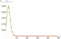
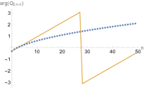
(a) $\beta=1/3,t=-1$

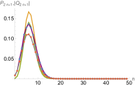
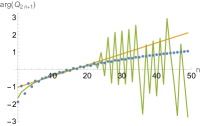
(b) $\beta=0.95,t=-1$

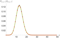
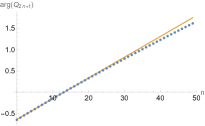
(c) $\beta=1/3,t=-3$

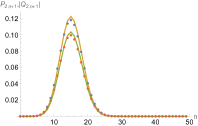
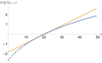
(d) $\beta=0.95,t=-3$

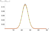
(e) $\beta=1/3,t=-7$

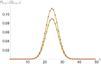
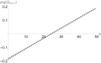
(f) $\beta=0.95,t=-7$

Figure 1: The comparison between the simplified saddle approximation and exact results with $N=100$ and for high temperature $\beta=1/3$ (a,c,e) and intermediate temperature $\beta=0.95<\beta_{c}$ (b,d,f). In the $P_{2n+1},|Q_{2n+1}|$ plots, the blue dots are exact values of $P_{2n+1}$ and the red dots are exact values of $|Q_{2n+1}|$; the yellow joint lines are saddle approximation of $P_{2n+1}$ and the green joint lines are saddle approximation of $|Q_{2n+1}|$. In the $\arg Q_{2n+1}$ plots, the blue dots are exact values of $\arg Q_{2n+1}$ and the yellow joint lines are saddle approximation of $\arg Q_{2n+1}$. In (b) where the simplified saddle approximation does not work very well, we plot the saddle approximation using (74). The purple joint line is $P_{2n+1},$the gray joint line is $|Q_{2n+1}|$ in the left picture, and the green joint line is $\arg Q_{2n+1}$ in the right picture. For $n$ not too big, the saddle approximation is improved, but for large $n$ it loses accuracy and we need to improve the saddle location $x_{0}$ further in (74).

Similarly, for size winding, we have

$$e^{-\mu N/2}\overline{g_{\mu}(\tau)} =\frac{e^{-\beta^{2}/4}e^{-\mu N/2}\Gamma(N/2)}{2\sqrt{a^{\prime}\pi}}\int dx\sum_{i_{1}=0}^{N/2-1}\frac{(\cosh\mu)^{N/2-i_{1}-1}(\sinh\mu)^{i_{1}}}{i_{1}!(N/2-1-i_{1})!}e^{-\frac{1}{a^{\prime}}x^{2}+(2x+b^{\prime\prime})i_{1}}$$

$$=\frac{e^{-\beta^{2}/4}e^{-\mu}}{2^{N/2}\sqrt{a^{\prime}\pi}}\int dxe^{-\frac{1}{a^{\prime}}x^{2}}\left((1+e^{-2\mu})+(1-e^{-2\mu})e^{2x+b^{\prime\prime}}\right)^{N/2-1}$$ (79)

where

$$b^{\prime\prime}=\frac{(\beta+4\tau)^{2}}{4(N/2-1)}-\beta^{2}/4$$ (80)

The saddle approximation is the same as before, which sets $x_{0}=0$ in the leading order of small $\mu$. This leads to

$$\overline{Q_{2n+1}(t)}=\frac{e^{-\beta^{2}/4}}{2^{N/2-1}}C_{N/2-1}^{n}(1+e^{-b_{q}(t)})^{N/2-1-n}(1-e^{-b_{q}(t)})^{n},\quad b_{q}(t)=\frac{16t^{2}-\beta^{2}-8i\beta t}{4(N/2-1)}+\beta^{2}/4$$ (81)

Note that the phase of $\overline{Q_{2n+1}(t)}$ is perfectly proportional to the size because $1+e^{-b_{q}(t)}$ has fixed phase $\phi_{1}$ and $1-e^{-b_{q}(t)}$ has fixed phase $\phi_{2}$, which together leads to the phase of (81) as $(N/2-1)\phi_{1}+(\phi_{2}-\phi_{1})n$, which is linear in size $2n+1$. By (81) the slope to $n$ of the phase is

$$\phi_{2}-\phi_{1}=\arg\frac{1-e^{-b_{q}(t)}}{1+e^{-b_{q}(t)}}\approx-\frac{4\beta t/N}{\sinh(\beta^{2}/4+(16t^{2}-\beta^{2})/(2N))}$$ (82)

which increases with $t$ until the scrambling scale and then decreases. A few numerics with $N=100$ in Figure 1 shows that the simplified saddle approximation (78) and (81) is quite good for high temperatures. One might complain that the saddle approximation for the phase of $Q_{2n+1}$ is not quite good for large and small $n$, especially at early time in Figure 1a. But this is not important because the dominant pieces are around the peak of the magnitude where the linearity matches well. As we decrease the temperature but still above the critical temperature $T_{c}$, the simplified saddle approximation does not work very well in the early times but then improves as time increases. From thermal scale ($\sim\beta$) to scrambling scale ($\sim\sqrt{N}$), the size distribution moves from small to large and eventually stabilizes around $N/2$; the phase of $Q_{2n+1}$ organizes itself from not quite linear to linear in $n$; and the slope of the phase also decays, which is consistent with (82).

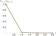
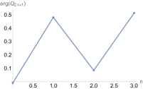
(a) $\beta=0.1,t=-0.1$

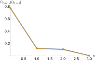
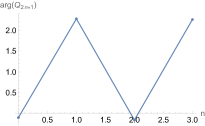
(b) $\beta=1,t=-0.1$

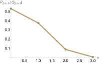
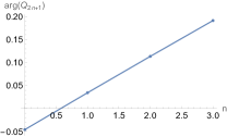
(c) $\beta=0.1,t=-0.6$

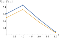
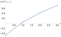
(d) $\beta=1,t=-0.8$

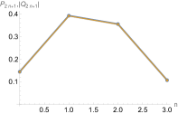
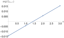
(e) $\beta=0.1,t=-1.5$

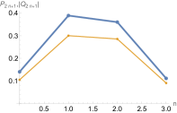
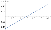
(f) $\beta=1,t=-1.5$

Figure 2: The exact results with $N=8$ and for high temperature $\beta=0.1$ (a,c,e) and low temperature $\beta=1$ (b,d,f). In the $P_{2n+1},|Q_{2n+1}|$ plots, the joint blue dots are exact values of $P_{2n+1}$ and the joint yellow dots are exact values of $|Q_{2n+1}|$. These two series of joint dots are plotted with different thicknesses for clear comparison. In the $\arg Q_{2n+1}$ plots, the joint blue dots are exact values of $\arg Q_{2n+1}$.

Besides the linearity of the phase of $Q_{2n+1}$, we also need to check if the phase of each individual size basis with the same size aligns. This can be measured by how $r_{n}=|Q_{n}|/P_{n}$ is close to one. With the numerical evidence in Figure 1, in the following, we will use the simplified saddle approximation (78) and (81) to estimate $r_{n}$ for all temperatures. we have

$$r_{2n+1}=e^{-\beta^{2}/4}\left|\frac{1+e^{-b_{q}(t)}}{1+e^{-b_{p}(t)}}\right|^{N/2-1-n}\left|\frac{1-e^{-b_{q}(t)}}{1-e^{-b_{p}(t)}}\right|^{n}$$ (83)

We approximate $e^{-b_{p}(t)}\approx e^{-\beta^{2}/4-8t^{2}/N}\left(1-\frac{\beta^{2}}{4(N/2-1)}\right)$ and $e^{-b_{q}(t)}\approx e^{-\beta^{2}/4-8t^{2}/N}\left(1+\frac{\beta^{2}+8i\beta t}{4(N/2-1)}\right)$, which leads to

$$r_{2n+1}\approx\exp\left[-\frac{\beta^{2}(1-e^{-\beta^{2}/4-8t^{2}/N})}{4(1+e^{-\beta^{2}/4-8t^{2}/N})}-\frac{\beta^{2}n}{N\sinh(\beta^{2}/4+8t^{2}/N)}\right]$$ (84)

Note that the second term in the exponent of (84) is not important in all scenarios. Since $\beta\sim O(1)$, at late times this term is exponentially suppressed, and at early times the dominant size is $n\sim O(1)$ and this term is of order $O(1/N)$. Keeping only the first exponent in (84) leads to the conclusion that $r_{2n+1}\sim e^{-\gamma\beta^{2}/4}$ where $\gamma\in[0,1]$, which implies that the size winding of commuting SYK model is near-perfect in high temperatures but damped as we decrease the temperature. When we cool down the system, the phase of the coefficients of the size basis with the same size starts to spread out from the perfectly alignment though their averaged phase is still proportional to the size. This estimate can be verified by the numeric result in Figure 1. In high temperatures, the difference between $P_{2n+1}$ and $|Q_{2n+1}|$ is quite small (a,c,e), but in lower temperature, the difference is larger (b,d,f) due to the overall suppression $e^{-\gamma\beta^{2}/4}$ as we just analyzed above. Therefore, we can confirm that the large $N$ commuting SYK model has size winding in high temperatures. As far as we know, this is the first nontrivial large $N$ non-holographic model that has near-perfect size winding.

As a comparison, we also show a case of small $N$ in Figure 2, where we take $N=8$. Since there is no sharp phase transition for finite $N$, here we choose the temperatures for best exhibiting the features regardless of $T_{c}$. As we can see from these plots, the small $N$ is indeed qualitatively the same as the large $N$ case though the thermal scale is not quite separable from the scrambling scale. The main difference is that for small $N$ at early time ($t\lesssim\beta$) the phases are poorly lined up for both low and high temperatures, but quickly reorganize themselves with linearity as time goes by. However, phase linearity only guarantees near-perfect size winding for high temperature because the magnitude of $Q_{2n+1}$ still matches with $P_{2n+1}$ in later times, while the magnitude of $Q_{2n+1}$ starts to drop off after the thermalization scale from $P_{2n+1}$ for lower temperature.

3.4 Peaked-size versus size-winding

In Schuster:2021uvg , there is another mechanism of teleportation in a generic scrambling system in high temperatures called peaked-size teleportation. This mechanism requires a narrow size distribution $P_{n}(t)$ of the scrambled operator $\psi_{j}^{r}(t)\rho_{r}^{1/2}$ around its average size $\mathcal{S}$. Such mechanism widely exists in many systems Schuster:2021uvg , including the late-time regime of a generic scrambling system when the dynamics can be approximated by Haar random unitaries Hayden:2007cs ; Roberts:2016hpo , random unitary circuits ($\geq 1D$) with local gates, random unitary circuits in $0D$ with all-to-all coupling and large $q$ SYK model in infinite temperature. The last two require encoding the to-be-scrambled qubit in terms of a large number of qubits. When the size distribution is peaked, in the sense that the ratio between size fluctuation and the size $\delta\mathcal{S}/\mathcal{S}\ll 1$, we can simply replace $e^{-\mu S}$ in both $K_{\mu}(t)$ and $G_{\mu}(t)$ as $e^{-\mu\mathcal{S}}$.

We can check if the commuting SYK model is peaked-size. The point is to compare the average size $\mathcal{S}$ and its variation $\delta\mathcal{S}$, which can be easily computed by $K_{\mu}(t)$

$$\mathcal{S}=-2\partial_{\mu}K_{\mu}(t)|_{\mu=0},\quad(\delta\mathcal{S})^{2}=2\partial_{\mu}^{2}K_{\mu}(t)|_{\mu=0}-\mathcal{S}^{2}$$ (85)

where the additional coefficient 2 is due to the normalization of $\psi_{j}^{r}(t_{r})\rho_{r}^{1/2}$. Since $K_{\mu}=e^{-\mu N/2}k_{\mu}$, we have

$$\mathcal{S}=Nk_{0}-2k{}_{0}^{\prime},\quad(\delta\mathcal{S})^{2}=2k_{0}^{\prime\prime}-4(k_{0}^{\prime})^{2}+2Nk_{0}^{\prime}(2k_{0}-1)-\frac{1}{2}N^{2}k_{0}(2k_{0}-1)$$ (86)

where prime is derivative to $\mu$. From (50) we have

$$k_{0} =\frac{1}{2},\quad k_{0}^{\prime}=\frac{1}{4}(N-2)e^{-\beta^{2}/4}e^{-8t^{2}/(N-2)}$$ (87)

$$k_{0}^{\prime\prime} =\frac{1}{4}(N-2)+\frac{1}{8}(N-2)(N-4)e^{-\frac{N-4}{2(N-2)}\beta^{2}}e^{-16t^{2}/(N-2)}$$ (88)

Let us consider the large $N$ limit. This leads to

$$\mathcal{S} \approx\frac{N}{2}(1-e^{-\beta^{2}/4}e^{-8t^{2}/N})$$ (89)

$$\delta\mathcal{S} \approx\frac{\sqrt{N}}{2}\left(2+(\beta^{2}-2)e^{-\beta^{2}/2}e^{-16t^{2}/N}\right)^{1/2}$$ (90)

where the ratio between size fluctuation and the size is $O(1/\sqrt{N})$. This $O(1/\sqrt{N})$ ratio can also be understood as a common feature of binary distribution (78) as long as $1\pm e^{-b_{p}(t)}\sim O(1)$. This analysis implies that the commuting SYK model should follow the mechanism of peaked size teleportation even though we see from Section 3.3 that size winding is also obeyed in high temperatures. There is no contradiction because size winding requires $Q_{n}(t)\approx P_{n}(t)e^{i(a_{1}+a_{2}n)}$ but does not impose any restriction on the distribution of $P_{n}(t)$. It is a little bit surprising that in the past work Schuster:2021uvg (and also Brown:2019hmk ; Nezami:2021yaq ), they are regarded as two distinct mechanisms, which are found in different (holographic versus non-holographic) models or exclusive regimes (e.g. low-temperature versus high-temperature SYK model).

Despite the ratio $\delta\mathcal{S}/\mathcal{S}$ is of order $O(1/\sqrt{N})$, as we will discuss in the next section, the teleportation protocol follows the peaked-size mechanism only for long time scale $t\sim O(\sqrt{N})$. For short time scale $t\sim O(1)$, the teleportation protocol works quite differently is related to thermalization.

4 Traversable wormhole teleportation protocol in commuting SYK

As the commuting SYK model shows near-perfect size winding in high temperature, it is natural to consier how it behaves in the traversable wormhole teleportation protocol Gao:2019nyj . It has been shown in Brown:2019hmk ; Nezami:2021yaq that the size winding is the microscopic mechanism for the teleportation through a traversable wormhole in the ordinary SYK model.

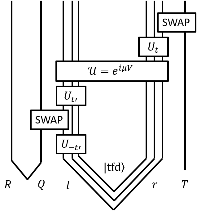
Figure 3: The traversable wormhole teleportation protocol (copied from Gao:2019nyj )

The quantum circuit of the traversable wormhole teleportation protocol is given by Figure 3, in which $U_{t}=e^{-iHt}$ is the evolution operator and SWAP works as an injection and extraction of the qubit being teleported. However, to study its effectiveness, computing a left-right causal correlator is sufficient. For fermionic system, this is defined as

$$C(t_{l},t_{r})=\left\langle\{e^{i\mu V}\psi_{j}^{l}(t_{l})e^{-i\mu V},\psi_{j}^{r}(t_{r})\}\right\rangle_{TFD}=-2\Im H_{i\mu}(t_{l},t_{r})$$ (91)

where we define the perturbed two-point function

$$H_{i\mu}(t_{l},t_{r})=-i\left\langle 0|\rho_{r}^{1/2}e^{i\mu V}\psi_{j}^{l}(t_{l})e^{-i\mu V}\psi_{j}^{r}(t_{r})\rho_{r}^{1/2}|0\right\rangle$$ (92)

For convenience, we compute the Euclidean version

$$h_{\mu}(\tau_{1},\tau_{2})=-i\left\langle 0|\rho_{r}^{1/2}e^{\mu V}\psi_{j}^{l}(\tau_{1})e^{-\mu V}\psi_{j}^{r}(\tau_{2})\rho_{r}^{1/2}|0\right\rangle$$ (93)

The computation is similar to Section 3 but more involved because we need to expand two exponentials $e^{\pm\mu V}$ in (93) and counting the number of terms with index conditions needs a finer analysis. We leave the computations ($q=4$) in Appendix A and just present the result here. We have

$$h_{\mu}(\tau_{1},\tau_{2})=h_{\mu}^{1}(\tau_{1},\tau_{2})+h_{\mu}^{2}(\tau_{1},\tau_{2})$$ (94)

where

$$h_{\mu}^{1} =\frac{e^{-\beta^{2}/4+(\tau_{1}+\tau_{2})^{2}}\cosh\mu}{2\sqrt{a\pi}}\int dxe^{-\frac{1}{a}x^{2}}\left(\cosh^{2}\mu-e^{-b_{1}}\sinh^{2}\mu-\sinh 2\mu\sinh\frac{\tau_{1}(2\tau_{2}+\beta)}{N/2-1}e^{2x-b_{2}}\right)^{N/2-1}$$ (95)

$$h_{\mu}^{2} =-\frac{e^{(\tau_{1}+\tau_{2})(\tau_{1}+\tau_{2}+\beta)}\sinh\mu}{2\sqrt{a\pi}}\int dxe^{-\frac{1}{a}x^{2}}\left(\cosh^{2}\mu-e^{-c_{1}}\sinh^{2}\mu-\sinh 2\mu\sinh\frac{2\tau_{1}\tau_{2}}{N/2-1}e^{2x-c_{2}}\right)^{N/2-1}$$ (96)

and a few parameters are defined as

$$a =\frac{\beta^{2}}{4(N/2-1)},\quad b_{1}=\frac{4\tau_{1}\tau_{2}}{N/2-1}\quad b_{2}=\frac{\tau_{2}(2\tau_{1}-\beta)+(N-4)\beta^{2}/8}{N/2-1}$$ (97)

$$c_{1} =\frac{2\tau_{1}(2\tau_{2}+\beta)}{N/2-1},\quad c_{2}=\frac{2\tau_{1}\tau_{2}+(\tau_{1}+\tau_{2})\beta+N\beta^{2}/8}{N/2-1}$$ (98)

4.1 Saddle approximation

Similar to Section 3.3, for large $N$ we can do the saddle approximation for the $x$ integral in $h_{\mu}^{i}$. In order to discuss the $\mu$ dependence, we will not restrict $\mu$ to be small. We will solve the saddle after analytic continuation $\mu\rightarrow i\mu$, $\tau_{1}\rightarrow it_{l}$ and $\tau_{2}\rightarrow it_{r}$. Up to a sign flip, from (95) and (96), we find that $C$ has $\mu$ periodicity of $\pi$. Therefore, we can restrict $\mu$ to the range of $[-\pi/2,\pi/2]$.

For $H_{i\mu}^{1}$ in large $N$ limit, we have

$$H_{i\mu}^{1}=\frac{e^{-\beta^{2}/4-(t_{l}+t_{r})^{2}}\cos\mu}{2\sqrt{a\pi}}\int dxe^{-\frac{1}{a}F_{1}(x)}$$ (99)

where $a=\beta^{2}/(2N)$ and

$$F_{1}(x)=x^{2}-\frac{\beta^{2}}{4}\log\left(\cos^{2}\mu+e^{\frac{4t_{l}t_{r}}{N/2}}\sin^{2}\mu+ie^{-\beta^{2}/4}\sin 2\mu\sinh\frac{2t_{l}t_{r}-i\beta t_{l}}{N/2}e^{\frac{2t_{l}t_{r}+i\beta t_{r}}{N/2}}e^{2x}\right)$$ (100)

In this equation, we have kept some $N$ dependence for later consideration for scales of $t_{l,r}$ up to $O(N)$. Taking derivative to $x$, we have the saddle equation

$$x=\frac{\beta^{2}}{4}\frac{ie^{-\beta^{2}/4}\sin 2\mu\sinh\frac{2t_{l}t_{r}-i\beta t_{l}}{N/2}e^{\frac{2t_{l}t_{r}+i\beta t_{r}}{N/2}}e^{2x}}{\cos^{2}\mu+e^{\frac{4t_{l}t_{r}}{N/2}}\sin^{2}\mu+ie^{-\beta^{2}/4}\sin 2\mu\sinh\frac{2t_{l}t_{r}-i\beta t_{l}}{N/2}e^{\frac{2t_{l}t_{r}+i\beta t_{r}}{N/2}}e^{2x}}$$ (101)

For teleportation, we consider $t_{l}>0$ and $t_{r}<0$, which leads to $t_{l}t_{r}<0$. Due to the overall exponential suppression factor $e^{-(t_{l}+t_{r})^{2}}$ in (99), we only need to consider the case $t_{l}+t_{r}\sim O(1)$. In the large $N$ limit, we have

$$i\sinh\frac{2t_{l}t_{r}-i\beta t_{l}}{N/2}e^{\frac{2t_{l}t_{r}+i\beta t_{r}}{N/2}} \approx\begin{cases}\frac{2it_{l}t_{r}+\beta t_{l}}{N/2}&t_{l}\sim-t_{r}\sim O(1)\\ \frac{i}{2}\left(e^{\frac{4t_{l}t_{r}}{N/2}}-1\right)&t_{l}\sim-t_{r}\gtrsim O(\sqrt{N})\end{cases}$$ (102)

where we considered two scales of $t_{l}\sim-t_{r}$. For the short time scale $t_{l}\sim-t_{r}\sim O(1)$, the saddle of $x$ is of order $1/N$ and we can approximate $e^{2x}\sim 1$ in leading order, which leads the solution to (101) as

$$x_{saddle}\approx\frac{\beta^{2}}{4}e^{-\beta^{2}/4}\sin(2\mu)\frac{2it_{l}t_{r}+\beta t_{l}}{N/2}$$ (103)

At this saddle point, we have in large $N$ limit

$$-\frac{1}{a}F_{1}(x_{saddle}) \approx 4t_{l}t_{r}\sin^{2}\mu+e^{-\beta^{2}/4}\sin(2\mu)(2it_{l}t_{r}+\beta t_{l})$$ (104)

$$F^{\prime\prime}_{1}(x_{saddle}) \approx 2$$ (105)

which leads to

$$H_{i\mu}^{1}=\frac{e^{-\beta^{2}/4-(t_{l}+t_{r})^{2}}\cos\mu}{2}\exp\left(4t_{l}t_{r}\sin^{2}\mu+e^{-\beta^{2}/4}\sin(2\mu)(2it_{l}t_{r}+\beta t_{l})\right)$$ (106)

For the long time scale where $t_{l}\sim-t_{r}$ is the same or higher order than $O(\sqrt{N})$ in (102), the saddle of $x$ is an $O(1)$ complex number, which gives an $O(1)$ value for $F_{1}(x_{saddle})$. These saddles do not have an analytic expression but we can easily find their values numerically. One can show numerically that the saddle leads to an $O(1)$ positive real part of $F_{1}(x_{saddle})$ for most choices in the parameter space. Due to large $1/a$ coefficient, $H_{i\mu}^{1}$ is exponentially suppressed in large $N$. An interesting exception is $\mu$ close to zero and scales as $1/N$. Let us assume $\mu=\mu_{0}/N$, and the saddle of $x$ in (101) is again of order $1/N$

$$x_{saddle}\approx\frac{i\mu_{0}\beta^{2}}{4N}e^{-\beta^{2}/4}\left(e^{\frac{4t_{l}t_{r}}{N/2}}-1\right)$$ (107)

At this saddle point, we have in large $N$ limit

$$-\frac{1}{a}F(x_{saddle}) \approx\frac{i}{2}e^{-\beta^{2}/4}\mu_{0}\left(e^{\frac{4t_{l}t_{r}}{N/2}}-1\right)$$ (108)

$$F^{\prime\prime}(x_{saddle}) \approx 2$$ (109)

which leads to

$$H_{i\mu}^{1}=\frac{e^{-\beta^{2}/4-(t_{l}+t_{r})^{2}}}{2}\exp\left(\frac{i\mu_{0}}{2}e^{-\beta^{2}/4}\left(e^{\frac{4t_{l}t_{r}}{N/2}}-1\right)\right)$$ (110)

Similarly, for $H_{i\mu}^{2}$ in large $N$ limit, we have

$$H_{i\mu}^{2}=-\frac{e^{i\beta(t_{l}+t_{r})-(t_{l}+t_{r})^{2}}i\sin\mu}{2\sqrt{a\pi}}\int dxe^{-\frac{1}{a}F_{2}(x)}$$ (111)

where

$$F_{2}(x)=x^{2}-\frac{\beta^{2}}{4}\log\left(\cos^{2}\mu+e^{\frac{4t_{l}t_{r}-2i\beta t_{l}}{N/2}}\sin^{2}\mu+ie^{-\beta^{2}/4}\sin 2\mu\sinh\frac{2t_{l}t_{r}}{N/2}e^{\frac{2t_{l}t_{r}-i\beta(t_{l}+t_{r})}{N/2}}e^{2x}\right)$$ (112)

Taking the derivative to $x$, we have the saddle equation

$$x=\frac{\beta^{2}}{4}\frac{ie^{-\beta^{2}/4}\sin 2\mu\sinh\frac{2t_{l}t_{r}}{N/2}e^{\frac{2t_{l}t_{r}-i\beta(t_{l}+t_{r})}{N/2}}e^{2x}}{\cos^{2}\mu+e^{\frac{4t_{l}t_{r}-2i\beta t_{l}}{N/2}}\sin^{2}\mu+ie^{-\beta^{2}/4}\sin 2\mu\sinh\frac{2t_{l}t_{r}}{N/2}e^{\frac{2t_{l}t_{r}-i\beta(t_{l}+t_{r})}{N/2}}e^{2x}}$$ (113)

Again due to the overall exponential suppression factor $e^{-(t_{l}+t_{r})^{2}}$ in (111), we only need to consider the case $t_{l}+t_{r}\sim O(1)$. In the large $N$ limit, we have

$$i\sinh\frac{2t_{l}t_{r}}{N/2}e^{\frac{2t_{l}t_{r}-i\beta(t_{l}+t_{r})}{N/2}} \approx\begin{cases}\frac{2it_{l}t_{r}}{N/2}&t_{l}\sim-t_{r}\sim O(1)\\ \frac{i}{2}\left(e^{\frac{4t_{l}t_{r}}{N/2}}-1\right)&t_{l}\sim-t_{r}\gtrsim O(\sqrt{N})\end{cases}$$ (114)

For the short time scale $t_{l}\sim-t_{r}\sim O(1)$, the saddle of $x$ is of order $1/N$

$$x_{saddle}\approx\frac{\beta^{2}}{4}e^{-\beta^{2}/4}\sin(2\mu)\frac{2it_{l}t_{r}}{N/2}$$ (115)

At this saddle point, we have in large $N$ limit

$$-\frac{1}{a}F_{2}(x_{saddle}) \approx(4t_{l}t_{r}-2i\beta t_{l})\sin^{2}\mu+e^{-\beta^{2}/4}\sin(2\mu)(2it_{l}t_{r})$$ (116)

$$F^{\prime\prime}_{2}(x_{saddle}) \approx 2$$ (117)

which leads to

$$H_{i\mu}^{2}=-\frac{e^{i\beta(t_{l}\cos 2\mu+t_{r})-(t_{l}+t_{r})^{2}}i\sin\mu}{2}\exp\left(4t_{l}t_{r}\sin^{2}\mu+e^{-\beta^{2}/4}\sin(2\mu)(2it_{l}t_{r})\right)$$ (118)

For the long time scale $t_{l}\sim-t_{r}\gtrsim O(\sqrt{N})$, the saddle is a complex $O(1)$ number, which can be shown numerically leading to positive real part of $F_{2}(x_{saddle})$ for most choices in the parameters space, which results in an exponentially suppressed $H_{i\mu}^{2}$ in large $N$ limit. The interesting exception is to consider $\mu=\mu_{0}/N$, which gives order one value saddle approximation for the integral (111). However, the $\sin\mu$ factor will be order $1/N$ and $H_{i\mu}^{2}$ is suppressed relative to $H_{i\mu}^{1}$.

Putting all together, we have for the short time scale $t_{l}\sim-t_{r}\sim O(1)$

$$H_{i\mu}= \frac{e^{-(t_{l}+t_{r})^{2}+4t_{l}t_{r}\sin^{2}\mu}}{2}\left[\cos\mu\exp\left(-\beta^{2}/4+e^{-\beta^{2}/4}\sin(2\mu)(2it_{l}t_{r}+\beta t_{l})\right)\right.$$

$$\left.-i\sin\mu\exp\left(e^{-\beta^{2}/4}\sin(2\mu)(2it_{l}t_{r})+i\beta(t_{l}\cos 2\mu+t_{r})\right)\right]$$ (119)

and for the long time scale $t_{l}\sim-t_{r}\gtrsim O(\sqrt{N})$

$$H_{i\mu}=\frac{e^{-\beta^{2}/4-(t_{l}+t_{r})^{2}}}{2}\exp\left(\frac{i\mu_{0}}{2}e^{-\beta^{2}/4}\left(e^{\frac{4t_{l}t_{r}}{N/2}}-1\right)\right)$$ (120)

Note that (119) has exponential decay as we send a signal earlier and receive the signal later, namely $t_{l}\sim-t_{r}\gg 1$, due to the factor $e^{-(t_{l}+t_{r})^{2}+4t_{l}t_{r}\sin^{2}\mu}$, while (120) tends to an $O(1)$ constant in the regime $t_{l}\sim-t_{r}\gg\sqrt{N}$. One should not be confused by this because in the long time scale (120), $\mu$ is been rescaled to $\mu_{0}/N$ that compensates the decaying effect of large time in the short time scale in the term $4t_{l}t_{r}\sin^{2}\mu$.

4.2 Sign of $\mu$

There is a crucial feature of the traversable wormhole teleportation that only one sign of $\mu$ allows the information sent through Gao:2019nyj . In the semiclassical picture, the sign of $\mu$ is proportional to the stress tensor of the injected matter that supports the traversable wormhole. The throat of a traversable wormhole opens only when the averaged null energy of the matter, which in turn is proportional to $\mu$, is negative Gao:2016bin . It is interesting to check if the teleportation in the commuting SYK model follows the same rule.

Since we have two distinct time scales, we need to discuss the dependence on the sign of $\mu$ separately. For the long time scale $t_{l}\sim-t_{r}\gtrsim O(\sqrt{N})$. It is interesting that the sign of $\mu$ does not affect the leading order magnitude of $C$. This can be seen easily using (120), which leads to

$$C(t_{l},t_{r})=e^{-\beta^{2}/4-(t_{l}+t_{r})^{2}}\sin\left(\frac{\mu_{0}}{2}e^{-\beta^{2}/4}\left(1-e^{\frac{4t_{l}t_{r}}{N/2}}\right)\right)$$ (121)

It is noteworthy that this formula holds for any temperature $T>T_{c}$ and scrambling time scale $O(\sqrt{N})$. This is very different from the large $N$ limit of the ordinary SYK model at scrambling time scale $O(\log N)$, which prefers positive $\mu$ in low temperature but has indifference in the sign of $\mu$ only in high temperature Gao:2019nyj .

As we discussed in Section 3.4 that the distribution is peaked in the sense $\delta\mathcal{S}/\mathcal{S}\ll 1$, we can find that (121) follows directly from the peaked-size mechanism Schuster:2021uvg . The result of the peaked-size teleportation is quite simple that the $e^{-i\mu V}$ in (92) measures the averaged size of $\psi_{j}^{r}(t_{r})\rho_{r}^{1/2}$ and becomes an exponential factor $e^{-i\mu(\mathcal{S}-N/2)}$ due to the narrow size distribution. It follows that

$$H_{i\mu}(t,-t)\approx G_{lr}(t,-t)\exp\left(-i\mu(\mathcal{S}+NG_{lr}(0,0)-N/2)\right)$$ (122)

where the first exponential $e^{i\mu V}$ simply factorizes as $e^{i\mu\left\langle V\right\rangle}=e^{-i\mu G_{lr}(0,0)}$ because it is a TOC. Taking (122) into (91), the left-right causal correlator has the form

$$C(t,-t)=2G_{lr}(t,-t)\sin\mu(\mathcal{S}+NG_{lr}(0,0)-N/2)$$ (123)

Note that the magnitude of $C$ is bounded by $G_{lr}(t_{l},t_{r})$ which decays as we drop the temperature. Therefore, the peaked-size teleportation works better in high temperatures. From (22), we can easily find that the left-right correlator in the commuting SYK model is given by

$$G_{lr}(t_{l},t_{r})\equiv-i\left\langle 0|\rho_{r}^{1/2}\psi_{j}^{l}(t_{l})\psi_{j}^{r}(t_{r})\rho_{r}^{1/2}|0\right\rangle=\frac{1}{2}e^{-\beta^{2}/4-(t_{l}+t_{r})^{2}}$$ (124)

Using (124) and (89), we see that (121) exactly matches with (123). For late time $t\rightarrow\infty$, we have $C(t,-t)=2G_{lr}(t,-t)\sin\mu NG_{lr}(0,0)$, which is the universal late-time behavior of “quantum traversable wormhole” due to the interference effect Gao:2018yzk , in which OTOCs simply vanish and TOCs factorize.

For the short time scale $t_{l}\sim-t_{r}\sim O(1)$, there is an obvious asymmetry for the flip $\mu\rightarrow-\mu$ from (119). To have a good exhibition of the sign effect, we can optimize the peak difference between $|\Im H_{i\mu}|$ and $|\Im H_{-i\mu}|$ for different temperatures in the range of $\mu\in[0,\pi/2]$ and $t_{r}<0$. The result is shown in Figure 4. From the plots, we find that in high temperature $\beta=0.1$, the sign difference is not large. Then as we decrease the temperature to an intermediate level $\beta=0.95$ but still in non-spin glass phase, the sign difference becomes large. In the both cases, we see that positive $\mu$ leads to a higher peak in $|H_{i\mu}|$ while negative $\mu$ gives a lower peak. Though this is qualitatively compatible with the analysis in large $q$ SYK model Gao:2019nyj that positive $\mu$ generates a negative energy shockwave into a black hole, we would like to emphasize again that the commuting SYK is not holographic. In particular, we do not see strong suppression of $\Im H_{i\mu}$ for negative $\mu$, which was observed in the large $q$ SYK model in the low temperature limit Gao:2019nyj . This means that for any nonzero $\mu$, there is always an $O(1)$ fidelity of teleportation.

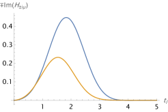
(a) $\beta=0.95$

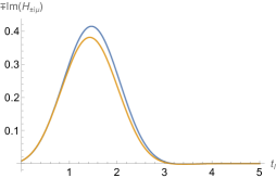
(b) $\beta=0.1$

Figure 4: The optimized $\max|\Im H_{i\mu}|-\max|\Im H_{-i\mu}|$ for the scale $t_{l}\sim-t_{r}\sim O(1)$. The blue curves are $-\Im H_{i\mu}$ and the yellow curves are $\Im H_{-i\mu}$. (a) Lower temperature $\beta=0.95$, the optimal $\mu=0.0468\pi$ and the injection time is at $t_{r}=-1.791$. (d) High temperature $\beta=0.1$, the optimal $\mu=0.0509\pi$ and the injection time is at $t_{r}=-1.507$.

Note that the sign difference in $C$ in the short time scale is completely different from the size-winding mechanism. Let us first recall why size winding prefers a specific sign (and indeed the value) of $\mu$ for teleportation. For the time scale larger than the thermalization scale, the exponential $e^{i\mu V}$ factorizes because it is a TOC piece Maldacena:2017axo

$$H_{i\mu}(t_{l},t_{r})\approx-ie^{i\mu\left\langle V\right\rangle}\left\langle 0|\rho_{r}^{1/2}\psi_{j}^{l}(t_{l})e^{-i\mu V}\psi_{j}^{r}(t_{r})\rho_{r}^{1/2}|0\right\rangle$$ (125)

where $\left\langle V\right\rangle$ is the expectation value in the thermofield double state. Given the size winding assumption $\psi_{j}^{r}(t)\rho_{r}^{1/2}=\frac{1}{\sqrt{2}}\sum_{I}|c_{I}(t)|e^{i(a_{1}(t)+a_{2}(t)|I|)}\Gamma_{I}$, (125) becomes

$$H_{i\mu}(t_{l},t_{r})\approx\frac{1}{2}e^{i\mu(\left\langle V\right\rangle+N/2)}\sum_{I}|c_{I}(t_{r})c_{I}(-t_{l})|e^{i(a_{1}(t_{r})+a_{1}(-t_{l})+(a_{2}(t_{r})+a_{2}(-t_{l})-\mu)|I|)}$$ (126)

If we take $t_{l}=-t_{r}$ and $\mu=2a_{2}(t_{r})$, we have $H_{i\mu}=\frac{1}{2}e^{i\theta}$ for a pure phase $\theta$. This guarantees the success of teleportation only for the specific sign (and also the value as a function of $t_{r}$) of $2a_{2}(t_{r})$ with an $O(1)$ imaginary part of $H_{i\mu}$. If we choose the opposite sign of $\mu$, each term in (126) will have a nonzero phase and the sum will be highly suppressed by the cancellation among terms, which leads to the failure of teleportation. From (82) we know that the slope to $n$ of the phase is $O(t/N)$ and $\mu$ should have been the same magnitude if the sign difference of $\mu$ were caused by size winding. However, in the short time scale and Figure 4, we have taken $N\rightarrow\infty$ but the optimal $\mu$ is still of order one.

To understand the sign difference of $\mu$ for finite $\beta$, let us first consider the high temperature limit $\beta\rightarrow 0$ in (119). We have

$$H_{i\mu}(t_{l},t_{r})=\frac{1}{2}e^{-(t_{l}+t_{r})^{2}+4t_{l}t_{r}\sin^{2}\mu}e^{i(2t_{l}t_{r}\sin 2\mu-\mu)}$$ (127)

which changes to its complex conjugate under $\mu\rightarrow-\mu$ and is consistent with Figure 4b. As we decrease the temperature from $\beta=0$, consider the small $\mu$ expansion in (119) with $t_{l}\sim-t_{r}$. The second line of (119) in leading order of $\mu$ is $-i\mu\exp(e^{-\beta^{2}/4}(2\mu)(-2it_{l}^{2}))$, which does not contribute to the sign difference of $\mu$ of $\Im H_{i\mu}$. For the first line of (119), in leading order of small $\beta$, we can rewrite it approximately as

$$H_{i\mu}\approx\frac{1}{2}e^{i\mu(-4t_{l}^{2}-2i\beta t_{l})}\approx-i\left\langle\psi^{l}_{j}(t_{l})\psi^{r}_{j}(-t_{l})\right\rangle e^{i\mu\left\langle[V,\psi^{l}_{j}(t_{l})]\psi^{r}_{j}(-t_{l})\right\rangle/\left\langle\psi^{l}_{j}(t_{l})\psi^{r}_{j}(-t_{l})\right\rangle+i\mu}$$ (128)

where the $\left\langle\cdots\right\rangle$ is evaluated in the thermofield double state at high temperature. In this equation, we have $\left\langle\psi^{l}_{j}(t_{l})\psi^{r}_{j}(-t_{l})\right\rangle\approx i/2$ (for $\beta=0$) and the exponent is the difference between a pair of OTOC and TOC

$$\left\langle[V,\psi^{l}_{j}(t_{l})]\psi^{r}_{j}(-t_{l})\right\rangle/\left\langle\psi^{l}_{j}(t_{l})\psi^{r}_{j}(-t_{l})\right\rangle \approx\sum_{i=1}^{N}-\frac{1}{2}-2\overline{W_{ji}}(it_{l}+\beta/2,\beta/2,it_{l},0)$$

$$\approx-4t_{l}^{2}-2i\beta t_{l}-1$$ (129)

where $\overline{W_{ji}}$ is the OTOC in (29), in which we expanded the exponent in leading order. The exponentiation of the difference between TOC and OTOC in (128) also exists in the regenesis phenomenon in 2d CFT Gao:2018yzk , though the latter is valid in a wider regime. The commutator (129) can be roughly understood as the “scattering” between $V$ and the pair of $\psi_{j}^{l}(t_{l})\psi_{j}^{r}(-t_{l})$. From (128), we see that the term linear in $\beta$ in the exponent contributes to the sign difference of $\mu$ because it gives an enhancement for positive $\mu$ and a suppression for negative $\mu$. As we discussed below (23), this linear in $\beta$ term is exactly the effective characteristic frequency $\beta\mathcal{J}^{2}$ by thermalization and reflects the underlying integrability of the commuting SYK model. As we decrease the temperature, the relative enhancement/suppression is stronger because the effective characteristic frequency is proportional to $\beta$. Though this analysis is for small $\beta$, it is compatible with the observation in Figure 4 for finite temperatures as long as we are still in non spin-glass phase. It is interesting to examine how the sign difference behaves if we drop the temperature below $T_{c}$ and enter the spin-glass phase. We leave this investigation to future work.

We can also compare the $O(1)$ time and high temperature result with the peaked-size formula (122). In early times, the size is $\mathcal{S}\approx 4t^{2}$ by (89). Comparing (122) with (128) at high temperature, it is easy to see that the quadratic term in the exponent in (128) is exactly the size $\mathcal{S}$. The piece beyond the peaked-size mechanism in this regime completely comes from the effective characteristic frequency $\beta\mathcal{J}^{2}$.

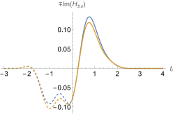
(a) $\beta=4$

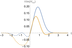
(b) $\beta=2.5$

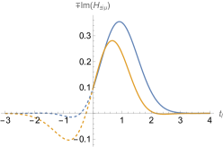
(c) $\beta=1$

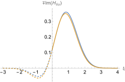
(d) $\beta=0.1$

Figure 5: The optimized $\max|\Im H_{i\mu}|-\max|\Im H_{-i\mu}|$ for $N=8$. The blue curves are $-\Im H_{i\mu}$ and the yellow curves are $\Im H_{-i\mu}$. The dashed lines are extended plots for $t_{l}<0$, which is an unphysical regime. (a) Even-lower temperature $\beta=4$, the optimal $\mu=0.221\pi$ and the injection time is at $t_{r}=-0.474$. (b) Low temperature $\beta=2.5$, the optimal $\mu=0.195\pi$ and the injection time is at $t_{r}=-0.614$. (c) Intermediate temperature $\beta=1$, the optimal $\mu=0.139\pi$ and the injection time is at $t_{r}=-0.720$. (d) High temperature $\beta=0.1$, the optimal $\mu=0.131\pi$ and the injection time is at $t_{r}=-0.742$.

On the other hand, one might be confused that why the short time scale does not follow the peaked-size mechanism given that $\delta\mathcal{S}/\mathcal{S}\sim O(1/\sqrt{N})$ even in early times. Indeed, the simple criterion $\delta\mathcal{S}/\mathcal{S}\ll 1$ is not always enough to guarantee peaked-size teleportation Schuster:2021uvg and sometimes we need a much finer criterion. For the current case, a simple explanation is that the peaked-size teleportation in Schuster:2021uvg assumes $\mu\sim O(1/K)$ for $K$ being a large number ($K$ could equal to $N$). Then the size fluctuation $\delta\mathcal{S}\sim O(\sqrt{K})$ only affects the phase of $e^{i\mu\mathcal{S}}$ by a negligible $O(1/\sqrt{K})$ amount. However, when we choose $\mu\sim O(1)$, the size fluctuation affects the phase by a large $O(\sqrt{K})$ amount and the peaked-size criterion must be much tighter.

As a comparison, we can also study the sign difference effect for small $N$ systems, which might be related to the recent simulation of traversable wormhole dynamics on the Sycamore quantum processor Jafferis:2022crx . For small $N$ the saddle approximation is poorly behaved, but the explicit expression of $H_{i\mu}$ can be easily written down by expanding the $N/2-1$ power term in both (95) and (96). We take $N=8$ and the numerics are straightforward. The optimized curves of $|\Im H_{i\mu}|-$$|\Im H_{-i\mu}|$ for a few choices of temperatures are shown in Figure 5.

For small $N$, different time scales are not separable and we only need to consider $t_{l,r}\sim O(1)$. Surprisingly, we find that the behavior of small $N$ in Figure 5 is qualitatively similar to the behavior of large $N$ in the short time scale in Figure 4. In all temperatures checked in Figure 5, positive $\mu$ leads to a higher maximum value than the negative $-\mu$. It is noteworthy that the dependence of the sign difference of $\mu$ on temperature follows a similar pattern as Figure 4, where we when cool down the system from high temperature, the sign difference becomes more visible until some critical temperature. If we continue to decrease the temperature, the sign difference is again diminished. This critical temperature seems to be the same order as the critical temperature $T_{c}=1$ for spin glass phase in the large $N$ case. Though we do not have a clean analysis of effective characteristic frequency for finite $N$ case, this similarity of sign difference suggest that the thermalization process of the commuting SYK model should play a crucial role. Moreover, as we drop the temperature from high to low, $\Im H_{i\mu}$ develops more and more peaks. To show the generation of new peaks, we extend the plot to an unphysical negative $t_{l}$ regime in Figure 5. For very large $\beta$ if we inject the signal around or earlier than $-\beta$, the plot of $\Im H_{i\mu}$ will have many wiggles, and the sign difference is not visible (which is not plotted here because the self-average result may not be reliable for too low temperatures).

4.3 Peak location and signal ordering

Another feature of a holographic model that is dual to a semiclassical traversable wormhole is the signal ordering Gao:2019nyj . If two signals are sent consecutively from the right side early enough to go through a traversable wormhole, they should be received on the left side with the same ordering of signals due to the smooth geometry in the traversable wormhole. This signal ordering preserving feature is unusual because the thermofield double state of two entangled black holes has maximal correlation at $t_{l}=-t_{r}$ due to the boost symmetry. This maximal correlation at opposite times on two sides indicates that the signal received time $t_{l}$ is approximately around $-t_{r}$, which leads to opposite signal ordering before scrambling time. Only when we send the signal in the time window for the semiclassical traversable wormhole throat, which is around scrambling time, the effects of two-sided instant coupling at $t=0$ generates a large enough backreaction that alters the signal ordering. This feature was verified in the large $q$ SYK model in low temperatures Gao:2019nyj .

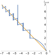
(a) $\beta=0.95$

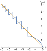
(b) $\beta=0.1$

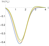
(c) $t_{r}\sim-1.6$

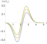
(d) $t_{r}\sim-2.2$

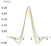
(e) $t_{r}\sim-2.8$

Figure 6: Signal ordering for the scale $t_{l}\sim-t_{r}\sim O(1)$ in large $N$ limit. The first row is the signal receiving time $t_{peak}$ as a function of signal sending time $t_{r}$ for different temperatures. The yellow straight line is the reference $t_{peak}=-t_{r}$. The choices of $\mu$ are the same as Figure 4 for both temperatures. The second row is the plot of $\Im H_{i\mu}$ as a function of $t_{l}$ for three consecutive signals sent around different times $t_{r}$ at high temperature $\beta=0.1$. In each figure, the blue, yellow and green curves are for the latest, middle and earliest signals respectively around $t_{r}$.

It is interesting that for the non-holographic commuting SYK model, we could also find some time regime, in which the signal ordering is preserved. We define the signal receiving time as the $t_{l}=t_{peak}$ at the highest peak of $H_{i\mu}$. Let us first take the large $N$ case. For short time scale, the solution to $\partial_{t_{l}}H_{i\mu}=0$ for (119) can be numerically solved and is shown in Figure 6. The first row is the signal receiving time $t_{peak}$ as a function of signal sending time $t_{r}$ for different temperatures. By definition, if the slope of the function $t_{peak}(t_{r})$ is positive, this means that the signal ordering is preserved at $t_{r}$. We also draw a yellow straight line as the reference $t_{peak}=-t_{r}$ to show the asymptotic reverse signal ordering. For convenience, we choose $\mu$ to be the same as Figure 4 for all three temperatures.

A few interesting features can be readily observed from the first row of Figure 6. First, the function $t_{peak}(t_{r})$ is split into many intervals, in which the signal orderings could be different. Second, as we increase the temperature, we see more times preserving signal ordering. But in all temperatures, the first time interval with the largest $t_{r}$ does not preserve the signal ordering. For the intermediate ($\beta=0.95$) and high ($\beta=0.1$) temperatures, starting from the second largest time interval of $t_{r}$, the signal ordering is preserved. Third, the function $t_{peak}(t_{r})$ is ambiguous between two neighboring intervals. This is because at these times multiple comparable peaks emerge and the highest peak has a discontinuous jump.

To have an intuitive picture of the signal peak, we draw the second row of Figure 6 for $\Im H_{i\mu}$ as a function of $t_{l}$ for three consecutive signals sent around different times $t_{r}$ at high temperature $\beta=0.1$. In each figure, the blue, yellow, and green curves are for the latest, middle and earliest signals respectively around $t_{r}$. In Figure 6c, the signal sending time $t_{r}\sim-1.6$ is chosen from the first interval of Figure 6b, which shows reverse signal ordering. In Figure 6d, the signal sending time $t_{r}\sim-2.2$ is chosen from the bordering regime between the first and second interval of Figure 6b, which shows comparable two peaks. In Figure 6e, the signal sending time $t_{r}\sim-2.8$ is chosen from the second interval of Figure 6b, which shows signal ordering is preserved.

This observation is indeed similar to the semiclassical traversable wormhole in the large $q$ SYK model in low temperature in the sense that the signal ordering will be preserved only when you send it early enough. However, the transition time occurs at scrambling time for large $q$ SYK with $\mu\sim O(1/N)$ but only at $O(1)$ time for the commuting SYK model with a much large $\mu\sim O(1)$. Furthermore, the preservation of signal ordering occurs in many intervals and only for intermediate and high temperatures in the commuting SYK model.

For the long time scale, we always have reverse signal ordering due to the simple formula (121). Let us define

$$t_{l}=-\sqrt{N/2}T+t,\quad t_{r}=\sqrt{N/2}T$$ (130)

which in large $N$ limit leads to

$$C=e^{-\beta^{2}/4-t^{2}}\sin\left[\frac{\mu_{0}}{2}e^{-\beta^{2}/4}\left(1-e^{-4T^{2}}\right)\right]$$ (131)

for a given $T<0$. The signal receiving time is the peak as a function of $t$, which is always at $t=0$. From (131), we can infer that the peak is in the form of Gaussian. If $\mu_{0}$ is large enough, the sending time is split into a few intervals that are separated by $T_{n}=-\frac{1}{2}\sqrt{\log\frac{1}{1-2\pi ne^{\beta^{2}/4}/\mu_{0}}}$ for $n\in\mathbb{Z}_{+}$, at which the signal vanishes $C=0$. The threshold of $\mu_{0}$ for the existence of such multiple intervals is $\mu_{0}\geq 2\pi e^{\beta^{2}/4}$.

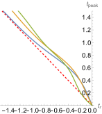
(a)

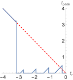
(b)

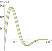
(c) $t_{r}\sim-0.35$

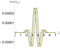
(d) $t_{r}\sim-3.35$

Figure 7: Signal ordering for $N=8$. (a) The signal receiving time $t_{peak}$ as a function of signal sending time $t_{r}$ for different temperatures. The blue, yellow, and green curves are for $\beta=0.1,1,2.5$ respectively. The red dashed line is the reference $t_{peak}=-t_{r}$. (b) Choose large $\mu=0.473\pi$ and $\beta=4$ leads to signal ordering preserved in early times. (c) $\Im H_{i\mu}$ in the signal ordering preserved regime. (d) $\Im H_{i\mu}$ in the signal ordering reversed regime. In both (c) and (d), blue, yellow, and green curves are for the latest, middle and earliest signals in the consecutive sequence of signals sent around $t_{r}$ with the same $\beta$ and $\mu$ as (b).

As a comparison, let us check the signal ordering for small $N$. We again take $N=8$ and the same parameters in Figure 5. The result is in Figure 7a, which shows that the signal ordering is reversed for all high ($\beta=0.1)$, intermediate ($\beta=1$) and low temperatures ($\beta=2.5$). This is compatible with the observation in Jafferis:2022crx that a one-time two-sided coupling is not strong enough to preserve the signal ordering for a learned commuting Hamiltonian with small $N$. While Jafferis:2022crx finely tuned the model by trotterized the one-time coupling into three times to achieve the preservation of signal ordering in some time range, here we can instead tune a large enough $\mu$ or $\beta$ to see a similar effect. Choosing $\mu$ close to $\pi/2$ and large $\beta$, we find that the signal ordering is preserved in early times as shown in Figure 7b. An illustration of $\Im H_{i\mu}$ in this regime for three consecutive signals sent around $t_{r}\sim-0.35$ is given by Figure 7c. However, such a regime is smaller than the thermal scale and quite transient, which is in essence quite different from the case for large $N$ and the short time scale case in Figure 6. The preservation of signal ordering is also piecewise in Figure 7b because there are multiple peaks competing as we send a signal toward earlier times. Roughly after the thermal scale $\beta$, we see from 7b that the signal ordering is reversed and obeys $t_{peak}=-t_{r}$ quite well. In this regime, we plot $\Im H_{i\mu}$ for three consecutive signals sent around $t_{r}\sim-3.35$ in Figure 7d as an example.

5 Conclusion and discussion

In this work, we studied the large $N$ limit of a variant of the SYK model whose Hamiltonian contains only commutative $q$-local interaction terms. There are many different ways to define such a commuting SYK-like Hamiltonian and we choose the simplest one by constructing each term in the Hamiltonian by a $q/2$ product of commutative ingredients $X_{i}=\psi_{2i-1}\psi_{2i}$ with a random coupling $\mathcal{J}_{I}$ that is drawn from a Gaussian ensemble. Since this model has infinite numbers of conserved charges in the large $N$ limit, it is integrable and completely solvable. It turns out that this model is non-holographic by checking its spectrum, two-point functions, and out-of-time-ordered correlators. Due to the large numbers of degrees of freedom in this model, an excitation $\psi_{i}$ thermalizes but in a way different from holographic models. In particular, its thermalization has two features: it has a non-holographic Gaussian tail decay in two-point function, and an oscillation with effective characteristic frequency $\beta\mathcal{J}^{2}$, which is the typical energy of the excitation $\psi_{i}$ on a thermal state. The existence of this effective characteristic frequency reflects the underlying integrability of the commuting SYK model. This effective characteristic frequency also appears in four-point functions.

In spite of this, this model has some holography-like features, especially the near-perfect size-winding in high temperatures. It has been shown and also briefly reviewed in Section 3.2 that size-winding is a feature of holographic models but it is not known that any non-holographic models with size winding before this work. Nevertheless, the size winding in the commuting SYK model is quite different from the ordinary SYK model because it simultaneously has peaked-size distribution, to which the teleportation in the long time (scrambling) scale $t\gtrsim O(\sqrt{N})$ is attributed. Because of this, we would like to call the non-holographic commuting SYK model as pseudo-holographic.

Applying the traversable wormhole teleportation protocol to this commuting SYK model, we also find some similarities and differences with the ordinary SYK model. For large $N$, we find two different behaviors in short time scale $t\sim O(1)$ and long time scale $t\gtrsim O(\sqrt{N})$. In the short time scale, the sign of $\mu$ matters more and more as we decrease from infinite temperature but still above critical temperature $T_{c}=1$. A positive $\mu$ leads to a stronger signal transmission than the negative $-\mu$, which is compatible with the expectation of holography. However, the mechanism for the sign difference is neither size-winding nor peaked-size teleportation. Though the size is peaked in the sense that $\delta\mathcal{S}/\mathcal{S}\ll 1$, there is an important correction from the effective characteristic frequency $\beta\mathcal{J}^{2}$ that leads to the relative enhancement/suppression for the sign choice of $\mu$. This is a special feature of the thermalization of this model. On the other hand, the distinctions are also obvious that the time scale is much shorter than scrambling time $O(\sqrt{N})$, and it does not prohibit teleportation with negative $\mu$ in any temperatures, unlike the large $q$ SYK model in low temperatures. For the long time scale, we must take $\mu\sim O(1/N)$ and the sign of $\mu$ does not matter for teleportation efficiency for all $T>T_{c}$. In this case, the teleportation undergoes the peaked-size mechanism.

Besides the sign of $\mu$, the preservation of signal ordering also has interesting features. In the short time scale, there are many intervals that preserve the signal ordering with $O(1)$ value of $\mu$ turned on for intermediate and high temperatures above $T_{c}$. This is different from the semiclassical picture of the large $q$ SYK model, which preserves the signal ordering in low temperature with $\mu\sim O(1/N)$ and in scrambling time scale. On the other hand, the commuting SYK model always has reversed signal ordering in the long time scale.

As a comparison, we also numerically studied the small $N$ case and take $N=8$ as an example. Since $N$ is finite, there is only one time scale, in which the sign of $\mu$ matters as we drop from high temperature, which is qualitatively similar to the large $N$ case. As we decrease the temperature further, the sign difference disappears. The signal ordering is mostly reversed unless we tune large enough $\mu$ and $\beta$, in which we see quite transient reversed signal ordering in early times that are smaller than the thermal scale.

Below we end with a few discussions and comparisons with other related works.

Geometric picture of size winding

In the last section of Nezami:2021yaq , the authors suggested that the existence of size winding alone could potentially provide a geometrical picture for teleportation because one can heuristically identify the winding size distribution $Q_{n}(t)$ as the momentum wave function of a one-dimensional particle. However, the non-holographic essence of the commuting SYK model would give a strong constraint on the interpretation of such a geometric picture if it could be defined explicitly. Another aspect to note is that the argument for size winding in holographic systems Nezami:2021yaq is based on the near-AdS₂ isometry, which exists near the horizon of a semiclassical near-extremal black hole, which usually occurs in low temperature. But in the commuting SYK model, the size winding occurs at high temperatures and becomes damped when we decrease the temperature. This suggests that the size winding of the two types is from two different microscopic origins. This is a very interesting direction that we leave for future investigation.

Comparison with the learned SYK Hamiltonian

It is interesting to compare the $N=8$ ensemble averaged size winding result in Section 3.3 with the learned commuting SYK model in Jafferis:2022crx (and also follow-ups Kobrin:2023rzr ; Jafferis:2023moh ). The learnt Hamiltonian in Jafferis:2022crx consists of five terms

$$H=-0.36\psi_{1}\psi_{2}\psi_{4}\psi_{5}+0.19\psi_{1}\psi_{3}\psi_{4}\psi_{7}-0.71\psi_{1}\psi_{3}\psi_{5}\psi_{6}+0.22\psi_{2}\psi_{3}\psi_{4}\psi_{6}+0.49\psi_{2}\psi_{3}\psi_{5}\psi_{7}$$ (132)

Note that this commuting Hamiltonian can not be written in terms of (4) because the five terms do not share the same set of commuting ingredients $X_{i}$. However, it can be separated into two commuting groups, each of which shares a set of commuting ingredients. Nevertheless, comparing (132) with our $N=8$ model is still qualitatively reasonable. The main reason is that multiple groups of shared commuting ingredients just splits one $F$ into multiple commutative factors, and the counting in Section 3.1 and 3.2 mostly care about how many commuting terms of different overlap types in the Hamiltonian. Since $N=8,q=4$ allows at most $C_{N/2}^{q/2}=6$ terms, which is close to 5, we should expect qualitatively close behavior.

Let us simply fit the five coefficients of (132) with Gaussian distribution by comparing the moments, which gives $-0.034$ mean value and fluctuation $\sigma=0.436$. Comparing with (5) for $N=8$ and $q=4$, we have $\mathcal{J}=0.267$. In Jafferis:2022crx , the size winding is mainly checked at $\beta=4$ and $t_{r}=-2.8$ with $\mu=12/(4\times 7)=0.429$, which in our notation is $\beta_{\text{\text{here}}}=\beta_{\text{there}}\mathcal{J}=1.07$ and $t_{r,\text{here}}=t_{r,\text{there}}\mathcal{J}=-0.748$. The size winding of close parameters is demonstrated in Figure 2d, which shows that the phases are almost lined up and the difference between $P_{2n+1}$ and $|Q_{2n+1}|$ is not quite large. The alignment of phases with the same size can be measured by the ratio $r_{2n+1}=|Q_{2n+1}|/P_{2n+1}$, which on the four data points in Figure 2d is $r_{2n+1}\gtrsim 0.8$. In Figure 5c, we optimized the difference between the peak of $|\Im H_{i\mu}|$ and the peak of $|\Im H_{-i\mu}|$ for $\beta=1$ by tuning parameters $\mu=0.139\pi\approx 0.437$ and $t_{r}=-0.72$. Note that the specific Hamiltonian (132) with $N=7$ was learnt in Jafferis:2022crx also by maximizing the sign difference of $\mu$ but for another closely related quantity, the mutual information between the reference system and the qubit receiver in the traversable wormhole teleportation protocol. An interesting coincidence is that the optimal parameters $t_{r}$ and $\mu$ are quite close between our commuting SYK model and Jafferis:2022crx .

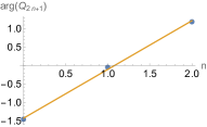
(a)

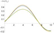
(b)

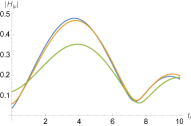
(c)

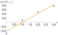
(d)

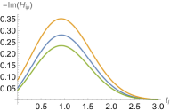
(e)

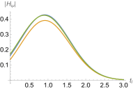
(f)

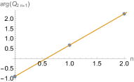
(g)

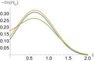
(h)

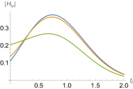
(i)

Figure 8: The first row is for the learned Hamiltonian in Jafferis:2022crx ; the second row is for the ensemble-averaged commuting SYK model with $N=8$, $\beta=1.07$ and $t=-0.748$ ($\mathcal{J}=1$); the third row is for the ensemble-averaged commuting SYK model with $N=6$, $\beta=1.9$ and $t=-0.475$ ($\mathcal{J}=1$). The left column is the phase of $Q_{2n+1}$ as a function of $n$. The yellow line is the linear fit of the three/four data points. The middle column is $-\Im H_{i\mu}$ for $\mu_{|H|}$ (blue), $\mu_{\Im H}$ (yellow) and $\mu_{\text{SW}}$ (green). The right column is $|H_{i\mu}|$ for $\mu_{|H|}$ (blue), $\mu_{\Im H}$ (yellow) and $\mu_{\text{SW}}$ (green).

However, if we look more carefully into these two models, we will see that the underlying mechanism is not completely due to size winding. Since the Hamiltonian (132) is given explicitly and each term is commutative to each other, it is quite straightforward to compute $H_{i\mu}$ and $Q_{2n+1}$ with (132) in Mathematica. We first compute the phase of $Q_{2n+1}(t)$ for $t=-2.8$ in Figure 8a, which is equivalent to Fig. 3d (or Fig. S15) in Jafferis:2022crx after shifting the first data point to the origin. We see that the three data points are aligned pretty well. The yellow straight line is the linear fit for these three points read as $Q_{2n+1}(-2.8)=-1.432+1.323n$. By the argument of size winding below (126), we should choose $\mu$ equal to half of the slope, namely $\mu_{\text{SW}}=0.662$, for best fidelity. On the other hand, we can maximize $|\Im H_{i\mu}|$ by finding the appropriate $t_{l}$ and $\mu$ given $t_{r}=-2.8$. It turns out that the optimal choice is $\mu_{\Im H}=0.463$ with $t_{l}=3.87$. By (126), if $e^{i\mu V}$ can be approximated by $e^{i\mu\left\langle V\right\rangle}$, the optimal $\mu$ for size winding should also give the maximal $|H_{i\mu}|$. Maximizing $|H_{i\mu}|$ by scanning $t_{l}$ and $\mu$ given $t_{r}=-2.8$, we find the optimal choice is $\mu_{|H|}=0.381$ with $t_{l}=3.71$. We plot the $-\Im H_{i\mu}$ and $|H_{i\mu}|$ in Figure 8b and 8c respectively for these three choices of $\mu$.

Clearly, these three optimal choices of $\mu$ are different. In particular, $\mu_{|H|}$ deviates from $\mu_{\text{SW}}$ quite much and is just $58\%$ of the latter. The explanation behind this distinction is that the size-winding mechanism is compatible with traversable wormhole teleportation only when the time scale is much larger than the thermal scale so that we can factorize out a pure phase in (126) by the argument of time-order-correlator. In this case $H_{i\mu}\propto G_{i\mu}$ and perfect size winding implies maximal $|H_{i\mu}|$. However, in the above example, $t_{r}=-2.8$, which is even shorter than the thermal scale $\beta=4$. Therefore we should expect the thermalization process to have an important interplay with the size winding and tunes the optimal $\mu$. The difference between $\mu_{\Im H}$ and $\mu_{|H|}$ is much subtler. Even for the factorized case (125), these two are not necessarily the same because the phase $e^{i\mu(\left\langle V\right\rangle+N/2)}$ exerts an additional rotation to $G_{i\mu}$, which will affect the imaginary part in a nontrivial way. However, in the known holographic large $q$ SYK model, one can check from Gao:2019nyj that these three $\mu$’s coincide in low temperature and equal to $-4\pi Ne^{-2\pi t/\beta}/(\beta\mathcal{J})$ (with the notation of Gao:2019nyj ).

If we check the same aspects with the ensemble-averaged commuting SYK model, we will find that thermalization also plays an important role. It has been discussed in Section 4.2 that in the short time scale and large $N$, thermalization is responsible for the sign difference of $\mu$ rather than size winding. In small $N$ cases in Figure 5, we see similar sign difference effect only when $t$ is comparable with $\beta$ for intermediate $\beta$. Though for small $N$ we have size winding with order one phase slope as shown in Figure 1, we now show that the size winding is not the complete mechanism for the sign difference. Let us take $N=8$, $\beta=1.07$ and $t=-0.748$ as an example. The phase of $Q_{2n+1}(-0.748)$ is shown in Figure 8d, where the four data points are mostly aligned. The yellow straight line is the linear fit for these three points read as $Q_{2n+1}(-0.748)=-0.430+0.425n$, which by size-winding assumption leads to $\mu_{\text{SW}}=0.213$. Maximizing $|\Im H_{i\mu}|$ leads to the optimal choice $\mu_{\Im H}=0.451$ with $t_{l}=0.929$. Maximizing $|H_{i\mu}|$ leads to the optimal choice $\mu_{|H|}=0.267$ with $t_{l}=0.912$. We plot the $-\Im H_{i\mu}$ and $|H_{i\mu}|$ in Figure 8e and 8f respectively for these three choices of $\mu$.

Here we see that these three $\mu$’s are different and the minimum $\mu_{\text{SW}}$ is just about 47% of the maximum $\mu_{\Im H}$. Compare the learned SYK model and the ensemble-averaged one, we see that the optimal $\mu$’s are different, the size-winding phase aligns better, and the peak of $\Im H_{i\mu}$ is slightly higher in the learned model. This is reasonable because the Hamiltonian (132) is especially learned to achieve the best teleportation fidelity for a specific operator $\psi_{1}$. For other operators $\psi_{i}$, the size-winding quality is worse at the same time Jafferis:2022crx ; Kobrin:2023rzr . On the other hand, the ensemble-averaged model works for all operators $\psi_{i}$ equally and shows an average level of teleportation efficiency.

As we argued before, the large deviation between $\mu_{|H|}$ and $\mu_{\text{SW}}$ for the learned Hamiltonian implies that the system is undergoing thermalization. For the ensemble-averaged model with equivalent parameter $\beta=1.07$, we see that $\mu_{|H|}$ is not far from $\mu_{\text{SW}}$, which means the thermalization is close to complete. This suggests that the effective temperature for the learned Hamiltonian is even lower than $1/\beta$, which strengthens the conclusion that thermalization plays a crucial role besides size-winding. To justify this, we tune the parameters in the ensemble-averaged model with lower temperature in the third row of Figure 6. We find that for $N=6$, $\beta=1.9$, and $t_{r}=-0.475$, the linearity of size-winding phase is pretty good with a large phase slope that gives $\mu_{\text{SW}}=0.785$ as shown in Figure 8g. At the same time, we find that $\mu_{\Im H}=0.570$ and $\mu_{|H|}=0.468$. On one hand, this is quite similar to the learned Hamiltonian case (the first row of Figure 8), including the relative ordering of three $\mu$’s ($\mu_{\text{SW}}>\mu_{\Im H}>\mu_{|H|}$ with $\mu_{|H|}/\mu_{\text{SW}}\approx 59.6\%$). On the other hand, the ratio $|t_{r}|/\beta=25\%$ suggests that the size-winding of the learned Hamiltonian occurs at the early stage of thermalization.

Non-commutative terms

The non-existence of non-commutative terms was discussed in Kobrin:2023rzr ; Jafferis:2023moh , where the main focus was on their effects on size winding. However, based on the observation of the commuting SYK model, we find that size winding is not a unique feature of holographic models. It can exist in the non-holographic commuting SYK model, though in long time scale and large $N$ it also has peaked size distribution. Clearly, we need to introduce non-commutative terms to save it from peaked size distribution in large $N$ limit and keep the size-winding feature at the same time. For small $N$ cases, there is no peaked size distribution and the size-winding also exists. However, teleportation does not completely follow the rule of size-winding, and thermalization becomes important.

Recent simulation of the dynamics of traversable wormholes in Jafferis:2022crx is an excellent start toward the project “quantum gravity in the lab”. However, given the holography-like features in the commuting SYK model, it is not obvious that the simulation in Jafferis:2022crx with $N=7$ is for the non-holographic commuting SYK model or the holographic full SYK model. To have a better simulation for the dynamics of traversable wormhole that is mostly due to non-peaked size winding, we must increase $N$, separate the thermal scale with scrambling scale, and consider times after thermalization. This indicates that we will not learn commuting Hamiltonian as we scale up the system. Otherwise, it will be peaked-size and non-holographic. On the other hand, non-commutative terms will bring challenges because the implementation steps of simulation will be more complicated. Therefore, to understand how to minimally introduce non-commutative terms while preserving essential holographic features (e.g. non-peaked size winding distribution, very close three optimal $\mu$’s, etc.) is crucial for future simulation studies.

On the theoretical side, understanding the non-commutative terms is equally important. As we know that the commuting SYK model has large numbers of conserved charges that are related to overly abundant symmetries of the system. However, in quantum gravity, we should have much fewer symmetries and most of them need to be explicitly broken by introducing the non-commutative terms. It is extremely interesting to construct a holographic theory by (perhaps minimally) breaking symmetries in steps and to understand their meaning in the dual gravity language.

Appendix A Computation of $h_{\mu}$

Expanding the two exponentials $e^{\pm\mu V}$ in (93), we have

$$h_{\mu}= -i\sum_{I,J}\tilde{K}_{IJ}\left\langle 0|F(-\beta/2)\Gamma_{I}^{l}\Gamma_{I}^{r}\psi_{j}^{l}(\tau_{1})\Gamma_{J}^{l}\Gamma_{J}^{r}\psi_{j}^{r}(\tau_{2})F(-\beta/2)|0\right\rangle$$

$$= -i\sum_{I,J}\tilde{K}_{IJ}i^{|I|}\left\langle 0|F_{|I\cap K|=\mathbb{Z}_{+}}(-\beta/2)F_{|I\cap K|=\mathbb{Z}_{-}}(\beta/2)\psi_{j}^{l}(\tau_{1})\Gamma_{J}^{l}\Gamma_{J}^{r}\psi_{j}^{r}(\tau_{2})F(-\beta/2)|0\right\rangle$$

$$= \sum_{I,J}\tilde{K}_{IJ}i^{|I|}\left\langle 0|F(-\tau_{1})\psi_{j}^{r}F_{|I\cap K|=\mathbb{Z}_{+}}(\tau_{1}-\beta/2)F_{|I\cap K|=\mathbb{Z}_{-}}(\tau_{1}+\beta/2)\Gamma_{J}^{l}\Gamma_{J}^{r}\psi_{j}^{r}(\tau_{2})F(-\beta/2)|0\right\rangle$$

$$= \sum_{I,J}\tilde{K}_{IJ}i^{|I|+|J|}(-)^{|J|}\text{Tr}_{r}\left(\Gamma_{J}^{r}F(-\tau_{1})\psi_{j}^{r}F_{|I\cap K|=\mathbb{Z}_{+}}(\tau_{1}-\beta/2)F_{|I\cap K|=\mathbb{Z}_{-}}(\tau_{1}+\beta/2)\Gamma_{J}^{r}F(\tau_{2})\psi_{j}^{r}F(-\tau_{2}-\beta/2)\right)$$

$$= \sum_{I,J}\tilde{K}_{IJ}i^{|I|+|J|}(-)^{|j\cap J|}\text{Tr}\left(F_{|I\cap K|=\mathbb{Z}_{+}}(\tau_{1}-\beta/2)F_{|I\cap K|=\mathbb{Z}_{-}}(\tau_{1}+\beta/2)F_{|J\cap K|=\mathbb{Z}_{+}}(\tau_{2})F_{|J\cap K|=\mathbb{Z}_{-}}(-\tau_{2})\right.$$

$$\left.\psi_{j}^{r}F_{|J\cap K|=\mathbb{Z}_{+}}(-\tau_{2}-\tau_{1}-\beta/2)F_{|J\cap K|=\mathbb{Z}_{-}}(\tau_{2}-\tau_{1}+\beta/2)\psi_{j}^{r}\right)$$

$$= \frac{1}{2}\sum_{I,J}\tilde{K}_{IJ}i^{|I|+|J|}(-)^{|j\cap J|}\text{Tr}\left(F_{|I\cap K|=\mathbb{Z}_{+}}(\tau_{1}-\beta/2)F_{|I\cap K|=\mathbb{Z}_{-}}(\tau_{1}+\beta/2)F_{j\in K,|J\cap K|=\mathbb{Z}_{+}}(2\tau_{2}+\tau_{1}+\beta/2)\right.$$

$$\left.F_{j\notin K,|J\cap K|=\mathbb{Z}_{+}}(-\tau_{1}-\beta/2)F_{j\in K,|J\cap K|=\mathbb{Z}_{-}}(-2\tau_{2}+\tau_{1}-\beta/2)F_{j\notin K,|J\cap K|=\mathbb{Z}_{-}}(-\tau_{1}+\beta/2)\right)$$ (133)

where $\tilde{K}_{IJ}=\frac{1}{Z}(\cosh\frac{\mu}{2})^{2N-|I|-|J|}(i\sinh\frac{\mu}{2})^{|I|+|J|}(-)^{|J|}$ and we can define

$$K_{IJ}=i^{|I|+|J|}\tilde{K}_{IJ}=\frac{1}{Z}(-)^{|I|}(\cosh\frac{\mu}{2})^{2N-|I|-|J|}(\sinh\frac{\mu}{2})^{|I|+|J|}$$ (134)

All $F$ terms in (133) can be factorized as a product of eight terms, which are summarized as Table 1. For each $F_{\text{condition}}(x)$, taking ensemble average leads to

$$\overline{F_{\text{condition}}(x)}=\exp\left(\frac{c_{\text{condition}}x^{2}\sigma^{2}}{2^{q+1}}\right)$$ (135)

Let us again consider $q=4$ and $j=1$. In order to count the terms correctly, we first separate the indices into 9 groups, each group includes a pattern of $X_{i}$ overlapping with $I$ and $J$. For each $X_{i}$, if it overlaps $a$ indices with $I$ and $b$ indices with $J$, we call it $(a,b)$ type, where $a,b=0,1,2$. We count each type as $i_{ab}$. For example, if $N=10$ and $I=\{1,3,4,5,6\}$ and $J=\{1,2,3,5,7,8\}$, we have $i_{12}=i_{02}=1,i_{21}=2$ and all other $i_{ab}=0$. It is easy to find the following relations

$$\sum_{ab}i_{ab}=N/2,\quad\sum_{ab}ai_{ab}=|I|,\quad\sum_{ab}bi_{ab}=|J|$$ (136)

To compute (133), besides the cases in Table 1, we need to consider more conditions, which depends on whether $X_{1}$ has overlap with $I$ and $J$. This is because under the condition $1\in K$ or $1\notin K$, the counting for $c_{\text{condition}}$ will be different. Before we proceed to the counting, let us first note a cancellation due to the factor $(-)^{|j\cap J|}$. If $|X_{1}\cap J|=1$, there are two cases $1\in J,2\notin J$ and $1\notin J,2\in J$. If we consider two $J$ of these two cases with all other indices to be identical, $c_{\text{condition}}$ is the same for all cases in Table 1. However, they will have the opposite sign due to $(-)^{|j\cap J|}$ and thus cancel each other exactly. Therefore, we only have the following 6 cases to consider: $|X_{1}\cap I|=\gamma,|X_{1}\cap J|=\delta$ with $\gamma=0,1,2$ and $\delta=0,2$, which are labelled by $(\gamma,\delta)$ in Table 2. The countings for all nontrivial #’s in Table 1 are as follows.

#	conditions	$x$
1	$j\notin K,|I\cap K|=\mathbb{Z}_{+},|J\cap K|=\mathbb{Z}_{+}$	$-\beta$
2	$j\notin K,|I\cap K|=\mathbb{Z}_{+},|J\cap K|=\mathbb{Z}_{-}$	0
3	$j\notin K,|I\cap K|=\mathbb{Z}_{-},|J\cap K|=\mathbb{Z}_{+}$	0
4	$j\notin K,|I\cap K|=\mathbb{Z}_{-},|J\cap K|=\mathbb{Z}_{-}$	$\beta$
5	$j\in K,|I\cap K|=\mathbb{Z}_{+},|J\cap K|=\mathbb{Z}_{+}$	$2(\tau_{1}+\tau_{2})$
6	$j\in K,|I\cap K|=\mathbb{Z}_{+},|J\cap K|=\mathbb{Z}_{-}$	$2(\tau_{1}-\tau_{2})-\beta$
7	$j\in K,|I\cap K|=\mathbb{Z}_{-},|J\cap K|=\mathbb{Z}_{+}$	$2(\tau_{1}+\tau_{2})+\beta$
8	$j\in K,|I\cap K|=\mathbb{Z}_{-},|J\cap K|=\mathbb{Z}_{-}$	$2(\tau_{1}-\tau_{2})$

Table 1: Eight cases for $F_{\text{condition}}(x)$.

	$c_{\text{condition}}$(for different $(\gamma,\delta)$)
#	$(0,0)$,$(2,0)$,$(0,2)$,$(2,2)$	$(1,0)$,$(1,2)$
1+4	$\frac{1}{2}(u-1)(u-2)+\frac{1}{2}v(v-1)$	$\frac{1}{2}u(u-1)+\frac{1}{2}(v-1)(v-2)$
5	$u-i_{11}-1$	$i_{10}+i_{12}-1$
6	$i_{01}+i_{21}$	$i_{11}$
7	$i_{10}+i_{12}$	$u-i_{11}$
8	$i_{11}$	$i_{01}+i_{21}$

Table 2: Counting for $c_{\text{condition}}$.

#1

For all $1\notin K$, we have two indices of $X_{k_{1}}$ and $X_{k_{2}}$ to choose from $2$ to $N/2$. We have 9 cases: $(|I\cap K|,|J\cap K|)=(0,0),(0,2),(2,0),(2,2),(4,0),(0,4),(4,2),(2,4),(4,4)$, which for $(\gamma,\delta)=(0,0)$ case contributes to $c_{\text{condition}}$ (the total choice of $k_{1}$ and $k_{2}$) respectively as $C_{i_{00}-1}^{2},C_{i_{01}}^{2}+i_{02}(i_{00}-1),C_{i_{10}}^{2}+i_{20}(i_{00}-1),i_{20}i_{02}+C_{i_{11}}^{2}+(i_{00}-1)i_{22}+i_{10}i_{12}+i_{01}i_{21},C_{i_{20}}^{2},C_{i_{02}}^{2},i_{20}i_{22}+C_{i_{21}}^{2},i_{02}i_{22}+C_{i_{12}}^{2},C_{i_{22}}^{2}$. Note that $i_{00}-1$ appears here because $k_{1,2}\neq 1$ in the $(\gamma,\delta)=(0,0)$ case. Summing over all cases leads to

$$c_{\text{condition}}= \frac{1}{2}\left[i_{00}^{2}+\left(2i_{02}+2i_{20}+2i_{22}-1\right)i_{00}+i_{01}^{2}+i_{10}^{2}+\left(i_{02}+i_{20}+i_{22}\right){}^{2}-i_{02}+\left(i_{11}-1\right)i_{11}\right.$$

$$\left.+\left(i_{12}-1\right)i_{12}+i_{10}\left(2i_{12}-1\right)-i_{20}+\left(i_{21}-1\right)i_{21}+i_{01}\left(2i_{21}-1\right)-i_{22}\right]_{i_{00}\rightarrow i_{00}-1}$$ (137)

For other $(\gamma,\delta)$, one just needs to replace the $i_{00}\rightarrow i_{00}-1$ with $i_{\gamma\delta}\rightarrow i_{\gamma\delta}-1$ in (137). One can check that $c_{\text{condition}}$ are identical for $(\gamma,\delta)=(1,0),(1,2)$, and also identical for $(\gamma,\delta)=(0,0),(0,2),(2,0),(2,2)$ but with a different value.

#4

We have 4 cases: $(|I\cap K|,|J\cap K|)=(1,1),(1,3),(3,1),(3,3)$, which for $(\gamma,\delta)=(0,0)$ case contributes to $c_{\text{condition}}$ respectively as $i_{10}i_{01}+(i_{00}-1)i_{11},i_{11}i_{02}+i_{12}i_{01},i_{11}i_{20}+i_{21}i_{10},i_{11}i_{22}+i_{12}i_{21}$. Summing over all cases leads to

$$c_{\text{condition}}= \left(i_{10}+i_{12}\right)\left(i_{01}+i_{21}\right)+i_{11}\left(i_{00}+i_{02}+i_{20}+i_{22}\right)|_{i_{00}\rightarrow i_{00}-1}$$ (138)

For other $(\gamma,\delta)$, one just needs to replace the $i_{00}\rightarrow i_{00}-1$ with $i_{\gamma\delta}\rightarrow i_{\gamma\delta}-1$ in (138). Again, we see that $c_{\text{condition}}$ are identical for $(\gamma,\delta)=(1,0),(1,2)$, and also identical for $(\gamma,\delta)=(0,0),(0,2),(2,0),(2,2)$ but with a different value.

#1+4

Since $x^{2}=\beta^{2}$ for both #1 and #4, we can add their $c_{\text{condition}}$ together and have

$$c_{\text{condition}}=\begin{cases}\frac{1}{2}(u-1)(u-2)+\frac{1}{2}v(v-1),&(\gamma,\delta)=(0,0),(0,2),(2,0),(2,2)\\ \frac{1}{2}u(u-1)+\frac{1}{2}(v-1)(v-2),&(\gamma,\delta)=(1,0),(1,2)\end{cases}$$ (139)

where

$$u=i_{00}+i_{02}+i_{20}+i_{22}+i_{11},\quad v=i_{10}+i_{12}+i_{01}+i_{21}$$ (140)

#5

For all $1\in K$ cases, we set $k_{1}=1$ and we only need to choose $k_{2}$ from 2 to $N/2$. For $(\gamma,\delta)=(0,0)$, we have four cases: $(|I\cap k_{2}|,|J\cap k_{2}|)=(0,0),(0,2),(2,0),(2,2)$, which contributes to $c_{\text{condition}}$ respectively as $i_{00}-1,i_{02},i_{20},i_{22}$. Similarly, for $(\gamma,\delta)=(2,0),(0,2),(2,2)$ cases, just need to replace $i_{00}-1$ with $i_{00}$ and $i_{\gamma\delta}$ with $i_{\gamma\delta}-1$. In all these cases, the total $c_{\text{condition}}$ are the same

$$c_{\text{condition}}=i_{00}+i_{02}+i_{20}+i_{22}-1$$ (141)

For $(\gamma,\delta)=(1,0)$, the counting is different and we have $(|I\cap k_{2}|,|J\cap k_{2}|)=(1,0),(1,2)$, which contributes to $c_{\text{condition}}$ respectively as $i_{10}-1,i_{12}$; For $(\gamma,\delta)=(1,2)$, the counting leads to the contribution to $c_{\text{condition}}$ respectively as $i_{10},i_{12}-1$. In both cases, the total $c_{\text{condition}}$ are the same

$$c_{\text{condition}}=i_{10}+i_{12}-1$$ (142)

#6

For $(\gamma,\delta)=(0,0),(2,0),(0,2),(2,2)$, we have four cases: $(|I\cap k_{2}|,|J\cap k_{2}|)=(0,1),(2,1)$, which contributes to $c_{\text{condition}}$ respectively as $i_{01},i_{21}$, which together gives

$$c_{\text{condition}}=i_{01}+i_{21}$$ (143)

For $(\gamma,\delta)=(1,0),(1,2)$, we have $(|I\cap k_{2}|,|J\cap k_{2}|)=(1,1)$, whose contribution to $c_{\text{condition}}$ is

$$c_{\text{condition}}=i_{11}$$ (144)

#7

For $(\gamma,\delta)=(0,0),(2,0),(0,2),(2,2)$, we have four cases: $(|I\cap k_{2}|,|J\cap k_{2}|)=(1,0),(1,2)$, which contributes to $c_{\text{condition}}$ respectively as $i_{10},i_{12}$, which together gives

$$c_{\text{condition}}=i_{10}+i_{12}$$ (145)

For $(\gamma,\delta)=(1,0),(1,2)$, we have $(|I\cap k_{2}|,|J\cap k_{2}|)=(0,0),(2,0),(0,2),(2,2)$, which contributes to $c_{\text{condition}}$ respectively as $i_{00},i_{20},i_{02},i_{22}$, which together gives

$$c_{\text{condition}}=i_{00}+i_{02}+i_{20}+i_{22}$$ (146)

#8

For $(\gamma,\delta)=(0,0),(0,2),(2,0),(2,2)$, we have $(|I\cap k_{2}|,|J\cap k_{2}|)=(1,1)$, whose contribution to $c_{\text{condition}}$ is

$$c_{\text{condition}}=i_{11}$$ (147)

For $(\gamma,\delta)=(1,0),(1,2)$, we have $(|I\cap k_{2}|,|J\cap k_{2}|)=(0,1),(2,1)$, whose contribution to $c_{\text{condition}}$ is

$$c_{\text{condition}}=i_{01}+i_{21}$$ (148)

Above results are summarized in Table 2.

The next step is to count the number $d_{\gamma,\delta}$ of configurations of $I$ and $J$ for given $i_{ab}$ and $(\gamma,\delta)$. This is staightforward and the result is

$$d_{\gamma,\delta}=\frac{i_{\gamma\delta}(N/2-1)!}{\prod_{ab}i_{ab}!}\prod_{ab}\left(\frac{4}{a!b!(2-a)!(2-b)!}\right)^{i_{ab}}\equiv i_{\gamma\delta}d(i_{ab})$$ (149)

In (133) $(\gamma,\delta)=(0,0),(2,0),(1,0)$ gives $(-)^{|j\cap J|}=1$ and $(\gamma,\delta)=(0,2),(2,2),(1,2)$ gives $(-)^{|j\cap J|}=-1$. Therefore, the net contribution from $(\gamma,\delta)=(0,0),(0,2),(2,0),(2,2)$ to (133) is

$$h_{\mu}^{1}= \frac{1}{2}\sum_{i_{ab}}K_{IJ}(i_{00}+i_{20}-i_{02}-i_{22})d(i_{ab})e^{\frac{\left[\frac{1}{2}(u-1)(u-2)+\frac{1}{2}v(v-1)\right]\beta^{2}+4(u-i_{11}-1)(\tau_{1}+\tau_{2})^{2}}{4(N/2-1)}}$$

$$\times e^{\frac{(i_{01}+i_{21})(2(\tau_{1}-\tau_{2})-\beta)^{2}+(i_{10}+i_{12})(2(\tau_{1}+\tau_{2})+\beta)^{2}+4i_{11}(\tau_{1}-\tau_{2})^{2}}{4(N/2-1)}})$$ (150)

and the net contribution from $(\gamma,\delta)=(1,0),(1,2)$ to (133) is

$$h_{\mu}^{2}= \frac{1}{2}\sum_{i_{ab}}K_{IJ}(i_{10}-i_{12})d(i_{ab})e^{\frac{\left[\frac{1}{2}(v-1)(v-2)+\frac{1}{2}u(u-1)\right]\beta^{2}+4(i_{10}+i_{12}-1)(\tau_{1}+\tau_{2})^{2}}{4(N/2-1)}}$$

$$\times e^{\frac{i_{11}(2(\tau_{1}-\tau_{2})-\beta)^{2}+(u-i_{11})(2(\tau_{1}+\tau_{2})+\beta)^{2}+4(i_{01}+i_{21})(\tau_{1}-\tau_{2})^{2}}{4(N/2-1)}}$$ (151)

where the sum over $i_{ab}$ is restricted to $\sum_{ab}i_{ab}=N/2$ and $K_{IJ}$ in terms of $i_{ab}$ is

$$K_{IJ}=\frac{1}{\overline{Z}}(-)^{\sum_{ab}ai_{ab}}(\cosh\frac{\mu}{2})^{2N-\sum_{ab}(a+b)i_{ab}}(\sinh\frac{\mu}{2})^{\sum_{ab}(a+b)i_{ab}}$$ (152)

For both (150) and (151), the exponents are fixed if we fix $u,w=i_{11},y=i_{01}+i_{21}$ and $z=i_{10}+i_{12}$. Therefore, we can sum over other degrees of freedom first without changing the exponents. The remaining numbers obey

$$u+y+z=u+v=N/2$$ (153)

For (150), it turns out that

$$h_{\mu}^{1}= (\cosh\frac{\mu}{2})^{2N}\sum_{u,v,w}\sum_{z+y=v}\frac{(-)^{z+w}2^{2w+v-1}(\tanh\frac{\mu}{2})^{2w+v}(1+\tanh^{2}\frac{\mu}{2})^{2u-2w+v}\Gamma(N/2)}{\overline{Z}\cosh\mu\Gamma(u-w)\Gamma(1+y)\Gamma(1+z)\Gamma(1+w)}$$

$$\times e^{\frac{y(2\tau_{12}-\beta)^{2}+z(2(\tau_{1}+\tau_{2})+\beta)^{2}}{4(N/2-1)}}e^{\frac{\left[\frac{1}{2}(u-1)(u-2)+\frac{1}{2}v(v-1)\right]\beta^{2}+4(u-w-1)(\tau_{1}+\tau_{2})^{2}+4w(\tau_{1}-\tau_{2})^{2}}{4(N/2-1)}}$$

$$= (\cosh\frac{\mu}{2})^{2N}\sum_{u,v}\sum_{w=0}^{u}\frac{(-)^{w+v}2^{2w+2v-1}(\tanh\frac{\mu}{2})^{2w+v}(1+\tanh^{2}\frac{\mu}{2})^{2u-2w+v}\Gamma(N/2)}{\overline{Z}\cosh\mu\Gamma(u-w)\Gamma(1+v)\Gamma(1+w)}e^{-\frac{w\tau_{1}\tau_{2}}{N/2-1}}$$

$$\times e^{\frac{\left[(u-1)(u-2)+v(v-1)\right]\beta^{2}/8+(u-1)(\tau_{1}+\tau_{2})^{2}+v(\tau_{1}^{2}+(\tau_{2}+\beta/2)^{2})}{N/2-1}}\left[\sinh\frac{\tau_{1}(2\tau_{2}+\beta)}{N/2-1}\right]^{v}$$

$$= (\cosh\frac{\mu}{2})^{2N}\sum_{u+v=N/2}\frac{(-)^{v}2^{2v-1}(\tanh\frac{\mu}{2})^{v}(1+\tanh^{2}\frac{\mu}{2})^{2u+v}\Gamma(N/2)}{\overline{Z}\cosh\mu\Gamma(u)\Gamma(1+v)}\left(1-e^{-\frac{4\tau_{1}\tau_{2}}{N/2-1}}\tanh^{2}\mu\right)^{u-1}$$

$$\times e^{\frac{\left[(u-1)(u-2)+v(v-1)\right]\beta^{2}/8+(u-1)(\tau_{1}+\tau_{2})^{2}+v(\tau_{1}^{2}+(\tau_{2}+\beta/2)^{2})}{N/2-1}}\left[\sinh\frac{\tau_{1}(2\tau_{2}+\beta)}{N/2-1}\right]^{v}$$

$$= (\cosh\mu)^{N-1}\sum_{v=0}^{N/2-1}\frac{(-)^{v}2^{v-1}(\tanh\mu)^{v}\Gamma(N/2)}{\Gamma(N/2-v)\Gamma(1+v)}\left(1-e^{-\frac{4\tau_{1}\tau_{2}}{N/2-1}}\tanh^{2}\mu\right)^{N/2-v-1}$$

$$\times\left[\sinh\frac{\tau_{1}(2\tau_{2}+\beta)}{N/2-1}\right]^{v}e^{\frac{v^{2}\beta^{2}/4-v(\tau_{2}(2\tau_{1}-\beta)+(N-4)\beta^{2}/8)}{N/2-1}}e^{-\beta^{2}/4+(\tau_{1}+\tau_{2})^{2}}$$ (154)

where in the last step we drop off $v=N/2$ term because $1/\Gamma(0)=0$. Smilarly, for (151), we have

$$h_{\mu}^{2}= (\cosh\frac{\mu}{2})^{2N}\sum_{u,v,w}\sum_{z+y=v}\frac{(-)^{z+w}2^{2w+v-1}(\tanh\frac{\mu}{2})^{2w+v}(1+\tanh^{2}\frac{\mu}{2})^{2u+v-2w}\Gamma(N/2)}{\overline{Z}\cosh\mu\Gamma(1+u-w)\Gamma(1+y)\Gamma(1+w)\Gamma(z)}$$

$$\times e^{\frac{y\tau_{12}^{2}+z(\tau_{1}+\tau_{2})^{2}}{N/2-1}}e^{\frac{\left[\frac{1}{2}(v-1)(v-2)+\frac{1}{2}u(u-1)\right]\beta^{2}-8w\tau_{1}(2\tau_{2}+\beta)+u(2(\tau_{1}+\tau_{2})+\beta)^{2}-4(\tau_{1}+\tau_{2})^{2}}{4(N/2-1)}}$$

$$= (\cosh\frac{\mu}{2})^{2N}\sum_{u,v}\sum_{w=0}^{u}\frac{(-)^{w+v}2^{2w+2v-2}(\tanh\frac{\mu}{2})^{2w+v}(1+\tanh^{2}\frac{\mu}{2})^{2u+v-2w}\Gamma(N/2)}{\overline{Z}\cosh\mu\Gamma(1+u-w)\Gamma(1+w)\Gamma(v)}$$

$$\times e^{-\frac{2w\tau_{1}(2\tau_{2}+\beta)}{N/2-1}}e^{\frac{\left[(v-1)(v-2)+u(u-1)\right]\beta^{2}/8+u(\tau_{1}+\tau_{2}+\beta/2)^{2}+(v-1)(\tau_{1}^{2}+\tau_{2}^{2})}{N/2-1}}\left[\sinh\frac{2\tau_{1}\tau_{2}}{N/2-1}\right]^{v-1}$$

$$= (\cosh\frac{\mu}{2})^{2N}\sum_{u+v=N/2}\frac{(-)^{v}2^{2v-2}(\tanh\frac{\mu}{2})^{v}(1+\tanh^{2}\frac{\mu}{2})^{2u+v}\Gamma(N/2)}{\overline{Z}\cosh\mu\Gamma(1+u)\Gamma(v)}\left(1-e^{-\frac{2\tau_{1}(2\tau_{2}+\beta)}{N/2-1}}\tanh^{2}\mu\right)^{u}$$

$$\times e^{\frac{\left[(v-1)(v-2)+u(u-1)\right]\beta^{2}/8+u(\tau_{1}+\tau_{2}+\beta/2)^{2}+(v-1)(\tau_{1}^{2}+\tau_{2}^{2})}{N/2-1}}\left[\sinh\frac{2\tau_{1}\tau_{2}}{N/2-1}\right]^{v-1}$$

$$= (\cosh\mu)^{N-1}\sum_{v=0}^{N/2-1}\frac{(-)^{v+1}2^{v-1}(\tanh\mu)^{v+1}\Gamma(N/2)}{\Gamma(N/2-v)\Gamma(v+1)}\left(1-e^{-\frac{2\tau_{1}(2\tau_{2}+\beta)}{N/2-1}}\tanh^{2}\mu\right)^{N/2-v-1}$$

$$\times\left[\sinh\frac{2\tau_{1}\tau_{2}}{N/2-1}\right]^{v}e^{\frac{v^{2}\beta^{2}/4-v(2\tau_{1}\tau_{2}+(\tau_{1}+\tau_{2})\beta+N\beta^{2}/8)}{N/2-1}}e^{(\tau_{1}+\tau_{2})(\tau_{1}+\tau_{2}+\beta)}$$ (155)

where in the last line we used $1/\Gamma(0)=0$ and shift $v\rightarrow v+1$.

As a consistency check, at $\mu=0$, we should get back to two point function $G(\beta/2-\tau_{1}-\tau_{2})$. From (154), this leaves one term with $v=0$, which gives

$$h_{\mu}^{1}=\frac{1}{2}e^{-\beta^{2}/4+(\tau_{1}+\tau_{2})^{2}}$$ (156)

From (155), we see no term survives under $\mu\rightarrow 0$. Comparing (156) with (21) (for $q=4$ and $\tau=\beta/2-\tau_{1}-\tau_{2}$), we see they exactly match.

To evaluate $h_{\mu}^{1}$ and $h_{\mu}^{2}$, we can rewrite the sum over $v$ in terms of Gaussian integral. Using the same trick (68), we can write the normalized (154) as

$$h_{\mu}^{1}= \frac{(\cosh\mu)^{N-1}}{2\sqrt{a\pi}}\left(1-e^{-\frac{4\tau_{1}\tau_{2}}{N/2-1}}\tanh^{2}\mu\right)^{N/2-1}e^{-\beta^{2}/4+(\tau_{1}+\tau_{2})^{2}}$$

$$\times\int dxe^{-\frac{1}{a}x^{2}}\sum_{v=0}^{N/2-1}\frac{\Gamma(N/2)}{\Gamma(N/2-v)\Gamma(1+v)}\left(-2\tanh\mu\frac{\sinh\frac{\tau_{1}(2\tau_{2}+\beta)}{N/2-1}}{1-e^{-\frac{4\tau_{1}\tau_{2}}{N/2-1}}\tanh^{2}\mu}e^{2x-\frac{(\tau_{2}(2\tau_{1}-\beta)+(N-4)\beta^{2}/8)}{N/2-1}}\right)^{v}$$

$$= \frac{e^{-\beta^{2}/4+(\tau_{1}+\tau_{2})^{2}}\cosh\mu}{2\sqrt{a\pi}}\int dxe^{-\frac{1}{a}x^{2}}\left(\cosh^{2}\mu-e^{-b_{1}}\sinh^{2}\mu-\sinh 2\mu\sinh\frac{\tau_{1}(2\tau_{2}+\beta)}{N/2-1}e^{2x-b_{2}}\right)^{N/2-1}$$ (157)

where

$$a =\frac{\beta^{2}}{4(N/2-1)},\quad b_{1}=\frac{4\tau_{1}\tau_{2}}{N/2-1}\quad b_{2}=\frac{\tau_{2}(2\tau_{1}-\beta)+(N-4)\beta^{2}/8}{N/2-1}$$ (158)

Similarly, we can write the normalized (155) as

$$h_{\mu}^{2}= -\frac{(\cosh\mu)^{N-1}\tanh\mu}{2\sqrt{a\pi}}\left(1-e^{-\frac{2\tau_{1}(2\tau_{2}+\beta)}{N/2-1}}\tanh^{2}\mu\right)^{N/2-1}e^{(\tau_{1}+\tau_{2})(\tau_{1}+\tau_{2}+\beta)}$$

$$\times\int dxe^{-\frac{1}{a}x^{2}}\sum_{v=0}^{N/2-1}\frac{\Gamma(N/2)}{\Gamma(N/2-v)\Gamma(1+v)}\left(-2\tanh\mu\frac{\sinh\frac{2\tau_{1}\tau_{2}}{N/2-1}e^{2x-\frac{(2\tau_{1}\tau_{2}+(\tau_{1}+\tau_{2})\beta+N\beta^{2}/8)}{N/2-1}}}{1-e^{-\frac{2\tau_{1}(2\tau_{2}+\beta)}{N/2-1}}\tanh^{2}\mu}\right)^{v}$$

$$= -\frac{e^{(\tau_{1}+\tau_{2})(\tau_{1}+\tau_{2}+\beta)}\sinh\mu}{2\sqrt{a\pi}}\int dxe^{-\frac{1}{a}x^{2}}\left(\cosh^{2}\mu-e^{-c_{1}}\sinh^{2}\mu-\sinh 2\mu\sinh\frac{2\tau_{1}\tau_{2}}{N/2-1}e^{2x-c_{2}}\right)^{N/2-1}$$ (159)

where

$$c_{1} =\frac{2\tau_{1}(2\tau_{2}+\beta)}{N/2-1},\quad c_{2}=\frac{2\tau_{1}\tau_{2}+(\tau_{1}+\tau_{2})\beta+N\beta^{2}/8}{N/2-1}$$ (160)

References

- (1) S. Sachdev and J. Ye, Gapless spin-fluid ground state in a random quantum heisenberg magnet, Physical Review Letters 70 (1993) 3339.
- (2) A. Kitaev, A simple model of quantum holography, in KITP strings seminar and Entanglement, vol. 12, 2015.
- (3) J. Maldacena and D. Stanford, Remarks on the Sachdev-Ye-Kitaev model, Phys. Rev. D 94 (2016) 106002 [1604.07818].
- (4) I. Danshita, M. Hanada and M. Tezuka, Creating and probing the Sachdev-Ye-Kitaev model with ultracold gases: Towards experimental studies of quantum gravity, PTEP 2017 (2017) 083I01 [1606.02454].
- (5) L. García-Álvarez, I.L. Egusquiza, L. Lamata, A. del Campo, J. Sonner and E. Solano, Digital Quantum Simulation of Minimal AdS/CFT, Phys. Rev. Lett. 119 (2017) 040501 [1607.08560].
- (6) D.I. Pikulin and M. Franz, Black Hole on a Chip: Proposal for a Physical Realization of the Sachdev-Ye-Kitaev model in a Solid-State System, Phys. Rev. X 7 (2017) 031006 [1702.04426].
- (7) A. Chen, R. Ilan, F. de Juan, D.I. Pikulin and M. Franz, Quantum holography in a graphene flake with an irregular boundary, Phys. Rev. Lett. 121 (2018) 036403 [1802.00802].
- (8) M. Brzezinska, Y. Guan, O.V. Yazyev, S. Sachdev and A. Kruchkov, Engineering SYK interactions in disordered graphene flakes under realistic experimental conditions, 2208.01032.
- (9) P. Uhrich, S. Bandyopadhyay, N. Sauerwein, J. Sonner, J.-P. Brantut and P. Hauke, A cavity quantum electrodynamics implementation of the Sachdev–Ye–Kitaev model, 2303.11343.
- (10) L. Susskind, Dear Qubitzers, GR=QM, 1708.03040.
- (11) A.R. Brown, H. Gharibyan, S. Leichenauer, H.W. Lin, S. Nezami, G. Salton et al., Quantum Gravity in the Lab. I. Teleportation by Size and Traversable Wormholes, PRX Quantum 4 (2023) 010320 [1911.06314].
- (12) S. Nezami, H.W. Lin, A.R. Brown, H. Gharibyan, S. Leichenauer, G. Salton et al., Quantum Gravity in the Lab. II. Teleportation by Size and Traversable Wormholes, PRX Quantum 4 (2023) 010321 [2102.01064].
- (13) J. Maldacena and L. Susskind, Cool horizons for entangled black holes, Fortsch. Phys. 61 (2013) 781 [1306.0533].
- (14) P. Gao and D.L. Jafferis, A traversable wormhole teleportation protocol in the SYK model, JHEP 07 (2021) 097 [1911.07416].
- (15) P. Gao, D.L. Jafferis and A.C. Wall, Traversable Wormholes via a Double Trace Deformation, JHEP 12 (2017) 151 [1608.05687].
- (16) A.M. García-García, Y. Jia, D. Rosa and J.J.M. Verbaarschot, Sparse Sachdev-Ye-Kitaev model, quantum chaos and gravity duals, Phys. Rev. D 103 (2021) 106002 [2007.13837].
- (17) S. Xu, L. Susskind, Y. Su and B. Swingle, A Sparse Model of Quantum Holography, 2008.02303.
- (18) D. Jafferis, A. Zlokapa, J.D. Lykken, D.K. Kolchmeyer, S.I. Davis, N. Lauk et al., Traversable wormhole dynamics on a quantum processor, Nature 612 (2022) 51.
- (19) B. Kobrin, T. Schuster and N.Y. Yao, Comment on ”Traversable wormhole dynamics on a quantum processor”, 2302.07897.
- (20) D. Jafferis, A. Zlokapa, J.D. Lykken, D.K. Kolchmeyer, S.I. Davis, N. Lauk et al., Comment on ”Comment on ”Traversable wormhole dynamics on a quantum processor” ”, 2303.15423.
- (21) D. Sherrington and S. Kirkpatrick, Solvable model of a spin-glass, Physical review letters 35 (1975) 1792.
- (22) D.J. Thouless, P.W. Anderson and R.G. Palmer, Solution of’solvable model of a spin glass’, Philosophical Magazine 35 (1977) 593.
- (23) G. Parisi, Infinite number of order parameters for spin-glasses, Physical Review Letters 43 (1979) 1754.
- (24) T. Schuster, B. Kobrin, P. Gao, I. Cong, E.T. Khabiboulline, N.M. Linke et al., Many-Body Quantum Teleportation via Operator Spreading in the Traversable Wormhole Protocol, Phys. Rev. X 12 (2022) 031013 [2102.00010].
- (25) B. Derrida, Random-energy model: Limit of a family of disordered models, Physical Review Letters 45 (1980) 79.
- (26) E. Gardner, Spin glasses with p-spin interactions, Nuclear Physics B 257 (1985) 747.
- (27) T.R. Kirkpatrick and D. Thirumalai, Dynamics of the structural glass transition and the p-spin—interaction spin-glass model, Physical review letters 58 (1987) 2091.
- (28) C.L. Baldwin and B. Swingle, Quenched vs Annealed: Glassiness from SK to SYK, Phys. Rev. X 10 (2020) 031026 [1911.11865].
- (29) V. Balasubramanian, M. DeCross, A. Kar, Y.C. Li and O. Parrikar, Complexity growth in integrable and chaotic models, JHEP 07 (2021) 011 [2101.02209].
- (30) B. Craps, M. De Clerck, O. Evnin, P. Hacker and M. Pavlov, Bounds on quantum evolution complexity via lattice cryptography, SciPost Phys. 13 (2022) 090 [2202.13924].
- (31) A.M. García-García and J.J.M. Verbaarschot, Spectral and thermodynamic properties of the Sachdev-Ye-Kitaev model, Phys. Rev. D 94 (2016) 126010 [1610.03816].
- (32) J.M. Deutsch, Eigenstate thermalization hypothesis, Reports on Progress in Physics 81 (2018) 082001 [1805.01616].
- (33) S.H. Shenker and D. Stanford, Black holes and the butterfly effect, JHEP 03 (2014) 067 [1306.0622].
- (34) A. Kitaev, Hidden correlations in the hawking radiation and thermal noise, in Talk given at the Fundamental Physics Prize Symposium, vol. 10, 2014.
- (35) D.A. Roberts and D. Stanford, Two-dimensional conformal field theory and the butterfly effect, Phys. Rev. Lett. 115 (2015) 131603 [1412.5123].
- (36) S.H. Shenker and D. Stanford, Multiple Shocks, JHEP 12 (2014) 046 [1312.3296].
- (37) S.H. Shenker and D. Stanford, Stringy effects in scrambling, JHEP 05 (2015) 132 [1412.6087].
- (38) J. Maldacena, S.H. Shenker and D. Stanford, A bound on chaos, JHEP 08 (2016) 106 [1503.01409].
- (39) B. Swingle and D. Chowdhury, Slow scrambling in disordered quantum systems, Phys. Rev. B 95 (2017) 060201 [1608.03280].
- (40) D.A. Roberts, D. Stanford and A. Streicher, Operator growth in the SYK model, JHEP 06 (2018) 122 [1802.02633].
- (41) X.-L. Qi and A. Streicher, Quantum Epidemiology: Operator Growth, Thermal Effects, and SYK, JHEP 08 (2019) 012 [1810.11958].
- (42) J. Maldacena, D. Stanford and Z. Yang, Diving into traversable wormholes, Fortsch. Phys. 65 (2017) 1700034 [1704.05333].
- (43) J. Maldacena and X.-L. Qi, Eternal traversable wormhole, 1804.00491.
- (44) H.W. Lin, J. Maldacena and Y. Zhao, Symmetries Near the Horizon, JHEP 08 (2019) 049 [1904.12820].
- (45) J. Maldacena, D. Stanford and Z. Yang, Conformal symmetry and its breaking in two dimensional Nearly Anti-de-Sitter space, PTEP 2016 (2016) 12C104 [1606.01857].
- (46) P. Hayden and J. Preskill, Black holes as mirrors: Quantum information in random subsystems, JHEP 09 (2007) 120 [0708.4025].
- (47) D.A. Roberts and B. Yoshida, Chaos and complexity by design, JHEP 04 (2017) 121 [1610.04903].
- (48) P. Gao and H. Liu, Regenesis and quantum traversable wormholes, JHEP 10 (2019) 048 [1810.01444].