Fairness Aware Counterfactuals for Subgroups

Abstract

In this work, we present Fairness Aware Counterfactuals for Subgroups (FACTS), a framework for auditing subgroup fairness through counterfactual explanations. We start with revisiting (and generalizing) existing notions and introducing new, more refined notions of subgroup fairness. We aim to (a) formulate different aspects of the difficulty of individuals in certain subgroups to achieve recourse, i.e. receive the desired outcome, either at the micro level, considering members of the subgroup individually, or at the macro level, considering the subgroup as a whole, and (b) introduce notions of subgroup fairness that are robust, if not totally oblivious, to the cost of achieving recourse. We accompany these notions with an efficient, model-agnostic, highly parameterizable, and explainable framework for evaluating subgroup fairness. We demonstrate the advantages, the wide applicability, and the efficiency of our approach through a thorough experimental evaluation of different benchmark datasets.

1 Introduction

Machine learning is now an integral part of decision-making processes across various domains, e.g., medical applications [22], employment [5, 7], recommender systems [28], education [25], credit assessment [4]. Its decisions affect our everyday life directly, and, if unjust or discriminative, could potentially harm our society [27]. Multiple examples of discrimination or bias towards specific population subgroups in such applications [32] create the need not only for explainable and interpretable machine learning that is more trustworthy [6], but also for auditing models in order to detect hidden bias for subgroups [29].

Bias towards protected subgroups is most often detected by various notions of fairness of prediction, e.g., statistical parity, where all subgroups defined by a protected attribute should have the same probability of being assigned the positive (favorable) predicted class. These definitions capture the explicit bias reflected in the model’s predictions. Nevertheless, an implicit form of bias is the difficulty for, or the burden [31, 20] of, an individual (or a group thereof) to achieve recourse, i.e., perform the necessary actions to change their features so as to obtain the favorable outcome [10, 34]. Recourse provides explainability (i.e., a counterfactual explanation [37]) and actionability to an affected individual, and is a legal necessity in various domains, e.g., the Equal Credit Opportunity Act mandates that an individual can demand to learn the reasons for a loan denial. Fairness of recourse captures the notion that the protected subgroups should bear equal burden [10, 14, 36, 20].

To illustrate these notions, consider a company that supports its promotion decisions with an AI system that classifies employees as good candidates for promotion, the favorable positive class, based on various performance metrics, including their cycle time efficiency (CTE) and the annual contract value (ACV) for the projects they lead. Figure 1(a) draws ten employees from the negative predicted class as points in the CTE-ACV plane and also depicts the decision boundary of the classifier. Race is the protected attribute, and there are two protected subgroups with five employees each, depicted as circles and triangles. For each employee, the arrow depicts the best action to achieve recourse, i.e., to cross the decision boundary, and the number indicates the cost of the action, here simply computed as the distance to the boundary [10]. For example, $x_{1}$ may increase their chances for promotion mostly by acquiring more high-valued projects, while $x_{2}$ mostly by increasing their efficiency. Burden is defined as the mean cost for a protected subgroup [31]. For the protected race 0, the burden is 2, while it is 2.2 for race 1, indicating thus unfairness of recourse against race 1. In contrast, assuming there is an equal number of employees of each race in the company, the classifier satisfies fairness of prediction in terms of statistical parity (equal positive rate in the subgroups).

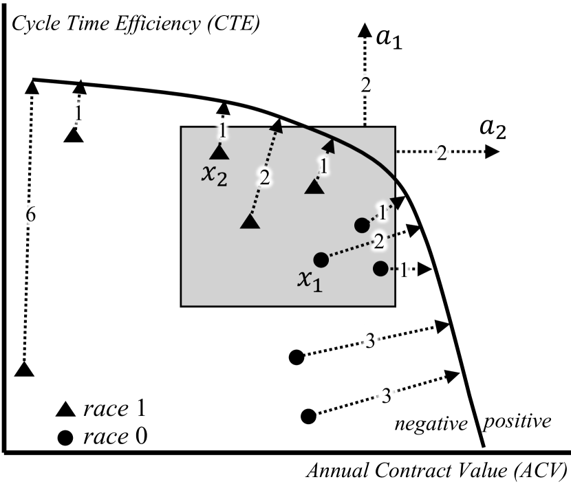
(a)

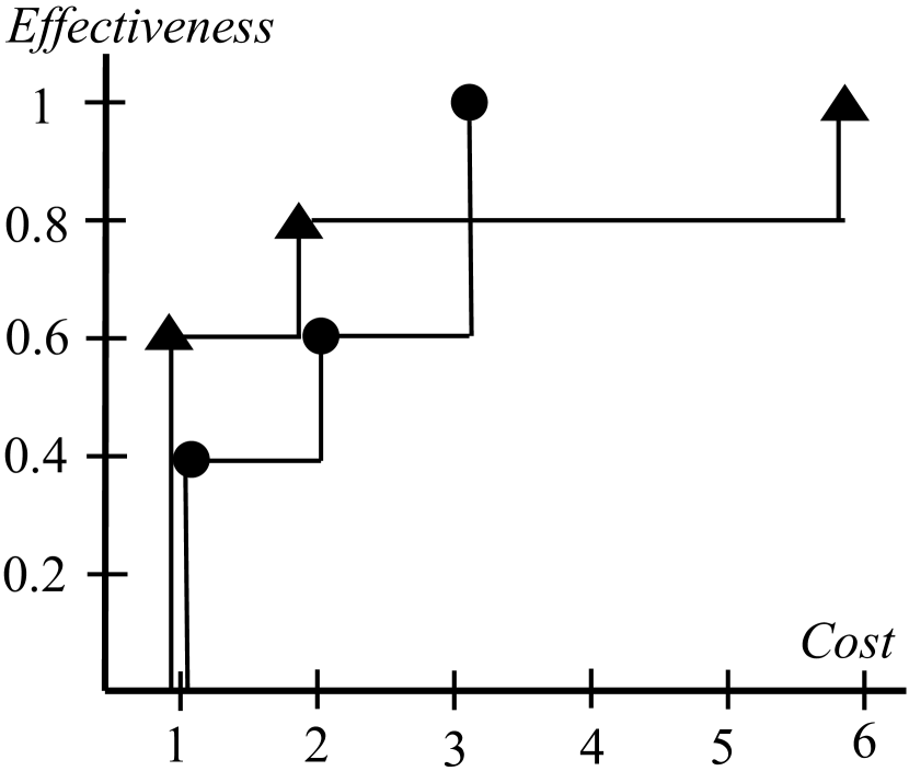
(b)

(c)

Figure 1: (a) An example of affected individuals, the decision boundary, actions, and a subpopulation (in the shaded region), depicted in the feature space; (b) Cumulative distribution of cost of recourse for the individuals in (a); (c) Comparison of two actions to achieve recourse for two individuals.

While fairness of recourse is an important concept that captures a distinct notion of algorithmic bias, as also explained in [14, 36], we argue that it is much more nuanced than the mean cost of recourse (aka burden) considered in all prior work [10, 31, 36, 20], and raise three issues.

First, the mean cost, which comprises a micro viewpoint of the problem, does not provide the complete picture of how the cost of recourse varies among individuals and may lead to contrasting conclusions. Consider again Figure 1(a), and observe that for race 1 all but one employee can achieve recourse with cost at most 2, while an outlier achieves recourse with cost 6. It is this outlier that raises the mean cost for race 1 above that of race 0. For the two race subgroups, Figure 1(b) shows the cumulative distribution of cost, termed the effectiveness-cost distribution ($\operatorname{\mathsf{ecd}}$) in Section 2. These distributions allow the fairness auditor to inspect the tradeoff between cost and recourse, and define the appropriate fairness of recourse notion. For example, they may consider that actions with a cost of more than 2 are unrealistic (e.g., because they cannot be realized within some timeframe), and thus investigate how many employees can achieve recourse under this constraint; we refer to this as equal effectiveness within budget in Section 2.3. Under this notion, there is unfairness against race 0, as only 60% of race 0 employees (compared to 80% of race 1) can realistically achieve recourse.

There are several options to go beyond the mean cost. One is to consider fairness of recourse at the individual level, and compare an individual with their counterfactual counterpart had their protected attribute changed value [36]. However, this approach is impractical as, similar to other causal-based definitions of fairness, e.g., [21], it requires strong assumptions about the causal structure in the domain [15]. In contrast, we argue that it’s preferable to investigate fairness in subpopulations and inspect the trade-off between cost and recourse.

Second, there are many cases where the aforementioned micro-level aggregation of individuals’ costs is not meaningful in auditing real-world systems. To account for this, we introduce a macro viewpoint where a group of individuals is considered as a whole, and an action is applied to and assessed collectively for all individuals in the group. An action represents an external horizontal intervention, such as an affirmative action in society, or focused measures in an organization that would change the attributes of some subpopulation (e.g., decrease tax or loan interest rates, increase productivity skills). In the macro viewpoint, the cost of recourse does not burden the individuals, but the external third party, e.g., the society or an organization. Moreover, the macro viewpoint offers a more intuitive way to audit a system for fairness of recourse, as it seeks to uncover systemic biases that apply to a large number of individuals.

To illustrate the macro viewpoint, consider the group within the shaded region in Figure 1(a). In the micro viewpoint, each employee seeks recourse individually, and both race subgroups have the same distribution of costs. However, we can observe that race 0 employees, like $x_{1}$ achieve recourse by actions in the ACV direction, while race 1 employees, like $x_{2}$ in the orthogonal CTE direction. This becomes apparent when we take the macro viewpoint, and investigate the effect of action $a_{1}$, depicted on the border of the shaded region, discovering that it is disproportionally effective on the race subgroups (leads to recourse for two-thirds of one subgroup but for none in the other). In this example, action $a_{1}$ might represent the effect of a training program to enhance productivity skills, and the macro viewpoint finds that it would perpetuate the existing burden of race 0 employees.

Third, existing notions of fairness of recourse have an important practical limitation: they require a cost function that captures one’s ability to modify one’s attributes, whose definition may involve a learning process [30], or an adaptation of off-the-shelf functions by practitioners [34]. Even the idea of which attributes are actionable, in the sense that one can change (e.g., one cannot get younger), or “ethical” to suggest as actionable (e.g., change of marital status from married to divorced) hides many complications [35].

Conclusions drawn about fairness of recourse crucially depend on the cost definition. Consider individuals $x_{1}$, $x_{2}$, and actions $a_{1}$, $a_{2}$, shown in Figure 1(c). Observe that is hard to say which action is cheaper, as one needs to compare changes within and across very dissimilar attributes. Suppose the cost function indicates action $a_{1}$ is cheaper; both individuals achieve recourse with the same cost. However, if action $a_{2}$ is cheaper, only $x_{2}$ achieves recourse. Is the classifier fair?

To address this limitation, we propose definitions that are oblivious to the cost function. The idea is to compare the effectiveness of actions to the protected subgroups, rather than the cost of recourse for the subgroups. One way to define a cost-oblivious notion of fairness of recourse is the equal choice for recourse (see Section 2.3), which we illustrate using the example in Figure 1(c). According to it, the classifier is unfair against $x_{1}$, as $x_{1}$ has only one option, while $x_{2}$ has two options to achieve recourse among the set of actions $\{a_{1},a_{2}\}$.

Contribution

Our aim is to showcase that fairness of recourse is an important and distinct notion of algorithmic fairness with several facets not previously explored. We make a series of conceptual and technical contributions.

Conceptually, we distinguish between two different viewpoints. The micro viewpoint follows literature on recourse fairness [10, 14, 36, 20] in that each individual chooses the action that is cheaper for them, but revisits existing notions. It considers the trade-off between cost and recourse, and defines several novel notions that capture different aspects of it. The macro viewpoint considers how an action collectively affects a group of individuals, and quantifies its effectiveness. It allows the formulation of cost-oblivious notions of recourse fairness. It also leads to an alternative trade-off between cost and recourse that may reveal systemic forms of bias.

Technically, we propose an efficient, interpretable, model-agnostic, highly parametrizable framework termed FACTS (Fairness-Aware Countefactuals for Subgroups) to audit for fairness of recourse. FACTS is efficient in computing the effectiveness-cost distribution, which captures the trade-off between cost and recourse, in both the micro or macro viewpoint. The key idea is that instead of determining the best action for each individual independently (i.e., finding their nearest counterfactual explanation [37]), it enumerates the space of actions and determines how many and which individuals achieve recourse through each action. Furthermore, FACTS employs a systematic way to explore the feature space and discover any subspace such that recourse bias exists among the protected subgroups within. FACTS ranks the subspaces in decreasing order of recourse bias it detects, and for each provides an interpretable summary of its findings.

Related Work

We distinguish between fairness of predictions and fairness of recourse. The former aims to capture and quantify unfairness by comparing directly the model’s predictions [26, 2] at: the individual level, e.g., individual fairness [9], counterfactual/causal-based fairness [21, 19, 25]; and the group level, e.g., demographic parity [38], equal odd/opportunity [12].

Fairness of recourse is a more recent notion, related to counterfactual explanations [37], which explain a prediction for an individual (the factual) by presenting the “best” counterfactual that would result in the opposite prediction, offering thus recourse to the individual. Best, typically means the nearest counterfactual in terms of a distance metric in the feature space. Another perspective, which we adopt here, is to consider the action that transforms a factual into a counterfactual, and specify a cost function to quantify the effort required by an individual to perform an action. In the simplest case, the cost function can be the distance between factual and counterfactual, but it can also encode the feasibility of an action (e.g., it is impossible to decrease age) and the plausibility of a counterfactual (e.g., it is out-of-distribution). It is also possible to view actions as interventions that act on a structural causal model capturing cause-effect relationships among attributes [15]. Hereafter, we adopt the most general definition, where a cost function is available, and assume that the best counterfactual explanation is the one that comes from the minimum cost action. Counterfactual explanations have been suggested as a mechanism to detect possible bias against protected subgroups, e.g., when they require changes in protected attributes [13].

Fairness of recourse, first introduced in [34] and formalized in [10], is defined at the group level as the disparity of the mean cost to achieve recourse (called burden in subsequent works) among the protected subgroups. Fairness of recourse for an individual is when they require the same cost to achieve recourse in the actual world and in an imaginary world where they would have a different value in the protected attribute [36]. This definition however only applies when a structural causal model of the world is available. Our work expands on these ideas and proposes alternate definitions that capture a macro and a micro viewpoint of fairness of recourse.

There is a line of work on auditing models for fairness of predictions at the subpopulation level [17, 18]. For example, [33] identifies subpopulations that show dependence between a performance measure and the protected attribute. [3] determines whether people are harmed due to their membership in a specific group by examining a ranking of features that are most associated with the model’s behavior. There is no equivalent work for fairness of recourse, although the need to consider the subpopulation is recognized in [16] due to uncertainty in assumptions or to intentionally study fairness. Our work is the first that audits for fairness of recourse at the subpopulation level.

A final related line of work is global explainability. For example, recourse summaries [30, 24] summarizes individual counterfactual explanations globally, and as the authors in [30] suggest can be used to manually audit for unfairness in subgroups of interest. [23] aims to explain how a model behaves in subspaces characterized by certain features of interest. [8] uses counterfactuals to unveil whether a black-box model, that already complies with the regulations that demand the omission of sensitive attributes, is still biased or not, by trying to find a relation between proxy features and bias. Our work is related to these methods in that we also compute counterfactual explanations for all instances, albeit in a more efficient manner, and with a specific goal.

2 Fairness of Recourse for Subgroups

2.1 Preliminaries

We consider a feature space $X=X_{1}\times\dots\times X_{n}$, where $X_{n}$ denotes the protected feature, which, for ease of presentation, takes two protected values $\{0,1\}$. For an instance $x\in X$, we use the notation $x.X_{i}$ to refer to its value in feature $X_{i}$.

We consider a binary classifier $h:X\to\{-1,1\}$ where the positive outcome is the favorable. For a given $h$, we are concerned with a dataset $D$ of adversely affected individuals, i.e., those who receive the unfavorable outcome. We prefer the term instance to refer to any point in the feature space $X$, and the term individual to refer to an instance from the dataset $D$.

We define an action $a$ as a set of changes to feature values, e.g., $a=\{\textit{country}\to\textit{US},\textit{education-num}\to 12\}$. We denote as $A$ the set of possible actions. An action $a$ when applied to an individual (a factual instance) $x$ results in a counterfactual instance $x^{\prime}=a(x)$. If the individual $x$ was adversely affected ($h(x)=-1$) and the action results in a counterfactual that receives the desired outcome ($h(a(x))=1$), we say that action $a$ offers recourse to the individual $x$ and is thus effective. In line with the literature, we also refer to an effective action as a counterfactual explanation for individual $x$ [37].

An action $a$ incurs a cost to an individual $x$, which we denote as $\operatorname{\mathsf{cost}}(a,x)$. The cost function captures both how feasible the action $a$ is for the individual $x$, and how plausible the counterfactual $a(x)$ is [14].

Given a set of actions $A$, we define the recourse cost $\operatorname{\mathsf{rc}}(A,x)$ of an individual $x$ as the minimum cost among effective actions if there is one, or otherwise some maximum cost represented as $c_{\infty}$:

$$\operatorname{\mathsf{rc}}(A,x)=\begin{dcases}\min\{\operatorname{\mathsf{cost}}(a,x)|a\in A:h(a(x))=1\},&\text{if\ }\exists a\in A:h(a(x))=1;\\ c_{\infty},&\text{otherwise}.\\ \end{dcases}$$

An effective action of minimum cost is also called a nearest counterfactual explanation [14].

We define a subspace $X_{p}\subseteq X$ using a predicate $p$, which is a conjunction of feature-level predicates of the form “feature-operator-value”, e.g., the predicate $p=(\textit{country}=\textit{US})\land(\textit{education-num}\geq 9)$ defines instances from the US that have more than 9 years of education.

Given a predicate $p$, we define the subpopulation group $G_{p}\subseteq D$ as the set of affected individuals that satisfy $p$, i.e., $G_{p}=\{x\in D|p(x)\}$. We further distinguish between the protected subgroups $G_{p,1}=\{x\in D|p(x)\land x.X_{n}=1\}$ and $G_{p,0}=\{x\in D|p(x)\land x.X_{n}=0\}$. When the predicate $p$ is understood, we may omit it in the designation of a group to simplify notation.

2.2 Effectiveness-Cost Trade-Off

For a specific action $a$, we naturally define its effectiveness ($\operatorname{\mathsf{eff}}$) for a group $G$, as the proportion of individuals from $G$ that achieve recourse through $a$:

$$\operatorname{\mathsf{eff}}(a,G)=\frac{1}{|G|}|\{x\in G|h(a(x))=1\}|.$$

We want to examine how recourse is achieved for the group $G$ through a set of possible actions $A$. We define the aggregate effectiveness ($\operatorname{\mathsf{aeff}}$) of $A$ for $G$ in two distinct ways.

In the micro viewpoint, the individuals in the group are considered independently, and each may choose the action that benefits itself the most. Concretely, we define the micro-effectiveness of set of actions $A$ for group $G$ as the proportion of individuals in $G$ that can achieve recourse through some action in $A$, i.e.,:

$$\operatorname{\mathsf{aeff_{\mu}}}(A,G)=\frac{1}{|G|}|\{x\in G|\exists a\in A,\operatorname{\mathsf{eff}}(a,x)=1\}|.$$

In the macro viewpoint, the group is considered as a whole, and an action is applied collectively to all individuals in the group. Concretely, we define the macro-effectiveness of set of actions $A$ for group $G$ as the largest proportion of individuals in $G$ that can achieve recourse through the same action in $A$, i.e.,:

$$\operatorname{\mathsf{aeff_{M}}}(A,G)=\max_{a\in A}\frac{1}{|G|}|\{x\in G|\operatorname{\mathsf{eff}}(a,x)=1\}|.$$

For a group $G$, actions $A$, and a cost budget $c$, we define the in-budget actions as the set of actions that cost at most $c$ for any individual in $G$:

$$A_{c}=\{a\in A|\forall x\in G,\operatorname{\mathsf{cost}}(a,x)\leq c\}.$$

We define the effectiveness-cost distribution ($\operatorname{\mathsf{ecd}}$) as the function that for a cost budget $c$ returns the aggregate effectiveness possible with in-budget actions:

$$\operatorname{\mathsf{ecd}}(c;A,G)=\operatorname{\mathsf{aeff}}(A_{c},G).$$

We use $\operatorname{\mathsf{ecd_{\mu}}}$, $\operatorname{\mathsf{ecd_{M}}}$ to refer to the micro, macro viewpoints of aggregate effectiveness.

The value $\operatorname{\mathsf{ecd}}(c;A,G)$ is the proportion of individuals in $G$ that can achieve recourse through actions $A$ with cost at most $c$. Therefore, the $\operatorname{\mathsf{ecd}}$ function has an intuitive probabilistic interpretation. Consider the subspace $X_{p}$ determined by predicate $p$, and define the random variable $C$ as the cost required by an instance $x\in X_{p}$ to achieve recourse. The function $\operatorname{\mathsf{ecd}}(c;A,G_{p})$ is the empirical cumulative distribution function of $C$ using sample $G_{p}$.

The inverse effectiveness-cost distribution function $\operatorname{\mathsf{ecd}}^{-1}(\phi;A,G)$ takes as input an effectiveness level $\phi\in[0,1]$ and returns the minimum cost required so that $\phi|G|$ individuals achieve recourse.

2.3 Definitions of Subgroup Recourse Fairness

We define recourse fairness of classifier $h$ for a group $G$ by comparing the $\operatorname{\mathsf{ecd}}$ functions of the protected subgroups $G_{0}$, $G_{1}$ in different ways.

The first two definitions are cost-oblivious, and simply compare the aggregate effectiveness of a set of actions of the protected subgroups.

Equal Effectiveness This definition has a micro and a macro interpretation, and says that the classifier is fair if the same proportion of individuals in the protected subgroups can achieve recourse: $\operatorname{\mathsf{aeff}}(A,G_{0})=\operatorname{\mathsf{aeff}}(A,G_{1})\,.$

Equal Choice for Recourse This definition has only a macro interpretation and claims that the classifier is fair if the protected subgroups can choose among the same number of sufficiently effective actions to achieve recourse, where sufficiently effective means the actions should work for at least $100\phi\%$ (for $\phi\in[0,1]$) of the subgroup:

$$|\{a\in A|\operatorname{\mathsf{eff}}(a,G_{0})\geq\phi\}|=|\{a\in A|\operatorname{\mathsf{eff}}(a,G_{1})\geq\phi\}|.$$

The next three definitions assume the $\operatorname{\mathsf{cost}}$ function is known, and have both a micro and a macro interpretation.

Equal Effectiveness within Budget The classifier is fair if the same proportion of individuals in the protected subgroups can achieve recourse with a cost at most $c$:

$$\operatorname{\mathsf{ecd}}(c;A,G_{0})=\operatorname{\mathsf{ecd}}(c;A,G_{1}).$$

Equal Cost of Effectiveness The classifier is fair if the minimum cost to achieve aggregate effectiveness of $\phi\in[0,1]$ in the protected subgroups is equal:

$$\operatorname{\mathsf{ecd}}^{-1}(\phi;A,G_{0})=\operatorname{\mathsf{ecd}}^{-1}(\phi;A,G_{1}).$$

Fair Effectiveness-Cost Trade-Off The classifier is fair if the protected subgroups have the same effectiveness-cost distribution, or equivalently for each cost budget $c$, their aggregate effectiveness is equal:

$$\max_{c}|\operatorname{\mathsf{ecd}}(c;A,G_{0})-\operatorname{\mathsf{ecd}}(c;A,G_{1})|=0.$$

The left-hand side represents the two-sample Kolmogorov-Smirnov statistic for the empirical cumulative distributions ($\operatorname{\mathsf{ecd}}$) of the protected subgroups. We say that the classifier is fair with confidence $\alpha$ if this statistic is less than $\sqrt{-\ln({\alpha}/2)\frac{|G_{p,0}|+|G_{p,1}|}{2|G_{p,0}||G_{p,1}|}}$.

The last definition takes a micro viewpoint and extends the notion of burden [31] from literature to the case where not all individuals may achieve recourse. The mean recourse cost of a group $G$,

$$\bar{\operatorname{\mathsf{rc}}}(A,G)=\frac{1}{|G|}\sum_{x\in G}\operatorname{\mathsf{rc}}(A,x)$$

considers individuals that cannot achieve recourse through $A$ and have a recourse cost of $c_{\infty}$. To exclude them, we denote as as $G^{*}$ the set of individuals of $G$ that can achieve recourse through an action in $A$, i.e., $G^{*}=\{x\in G|\exists a\in A,h(a(x))=1\}$. Then the conditional mean recourse cost is the mean recourse cost among those that can achieve recourse:

$$\bar{\operatorname{\mathsf{rc}}}^{*}(A,G)=\frac{1}{|G^{*}|}\sum_{x\in G^{*}}\operatorname{\mathsf{rc}}(A,x).$$

If $G=G^{*}$, the definitions coincide with burden.

Equal (Conditional) Mean Recourse The classifier is fair if the (conditional) mean recourse cost for the protected subgroups is the same:

$$\bar{\operatorname{\mathsf{rc}}}^{*}(A,G_{0};A)=\bar{\operatorname{\mathsf{rc}}}^{*}(A,G_{1}).$$

Note that when the group $G$ is the entire dataset of affected individuals, and all individuals can achieve recourse through $A$, this fairness notion coincides with fairness of burden [34, 31].

3 Fairness-aware Counterfactuals for Subgroups

This section presents FACTS (Fairness-aware Counterfactuals for Subgroups), a framework that implements both the micro and the macro viewpoint, and all respective fairness definitions provided in Section 2.3 to support auditing of the “difficulty to achieve recourse” in subgroups. The output of FACTS comprises population groups that are assigned (a) an unfairness score that captures the disparity between protected subgroups according to different fairness definitions and allows us to rank groups and (b) a user-intuitive, easily explainable counterfactual summary, which we term Comparative Subgroup Counterfactuals (CSC).

Figure 2 presents an example result of FACTS derived from the adult dataset [1]. The “if clause” represents the subgroup $G_{p}$, which contains all the affected individuals that satisfy the predicate $p=(\textit{hours-per-week = FullTime})\land(\textit{marital-status = Married-civ-spouse})\land(\textit{occupation = Adm-clerical})$. The information below the predicate refers to the protected subgroups $G_{p,0}$ and $G_{p,1}$ which are the female and male individuals of $G_{p}$ respectively. With blue color, we highlight the percentage $\operatorname{\mathsf{cov}}(G_{p,i})=|G_{p,i}|/|D_{i}|$ which serves as an indicator of the size of the protected subgroup. The most important part of the representation is the actions applied that appear below each protected subgroup and are evaluated in terms of fairness metrics. In this example, the metric is the Equal Cost of Effectiveness with effectiveness threshold $\phi=0.7$. For $G_{p,0}$ there is no action surpassing the threshold $\phi=0.7$, therefore we display a message accordingly. On the contrary, the action $a=\{\textit{hours-per-week}\to\textit{Overtime},\textit{occupation}\to\textit{Exec-managerial}\}$ has effectiveness $0.72>\phi$ for $G_{p,1}$, thus allowing a respective $72\%$ of the male individuals of $G_{p}$ to achieve recourse. The unfairness score is “inf”, since no recourse is achieved for the female subgroup.

⬇

If hours-per-week=FullTime,marital-status=Married-civ-spouse,occupation=Adm-clerical:

Protected Subgroup = ‘Male’, 1.87% covered

Make hours-per-week=Overtime@,occupation=Exec-managerial@ with effectiveness 72.00%

Protected Subgroup = ‘Female’, 1.80% covered

No recourses for this subgroup.

Bias against ‘Female’ due to Equal Cost of Effectiveness (threshold=0.7). Unfairness score = inf.

Figure 2: CSC for a highly biased subgroup in terms of Equal Cost of Effectiveness with $\phi=0.7$.

Method overview Deploying FACTS comprises three main steps: (a) Subgroup and action space generation, where frequent subgroups defined as frequent sets of feature-operator-value combinations in the affected population are derived and, respectively, frequent actions are collected in similar way from the unaffected population; (b) Counterfactual summaries generation, where proper matching of subgroups and actions is performed to produce valid counterfactual summaries for each subgroup and (c) CSC construction and fairness ranking, where each counterfactual summary is scored according to each definition from Section 2.3, producing a respective number of CSCs for each subgroup and allowing to produce separate subgroup rankings per definition. Next, we describe these steps in detail.

(a) Subgroup and action space generation Subgroups are generated by executing the fp-growth [11] frequent itemset mining algorithm on $D_{0}$ and on $D_{1}$ resulting to the sets of subgroups $\mathcal{G}_{0}$ and $\mathcal{G}_{1}$ and then by computing the intersection $\mathcal{G}=\mathcal{G}_{0}\bigcap\mathcal{G}_{1}$. In our setting, an item is a feature-level predicate of the form “feature-operator-value” and, consequently, an itemset is a predicate $p$ defining a subgroup $G_{p}$. This step guarantees that the evaluation in terms of fairness will be performed between the common subgroups $\mathcal{G}$ of the protected populations. The set of all actions $A$ is generated by executing fp-growth on the unaffected population to increase the chance of more effective actions and to reduce the computational complexity. The above process is parameterizable w.r.t. the selection of the protected attribute(s) and the minimum frequency threshold for obtaining candidate subgroups.

(b) Counterfactual summaries generation For each subgroup $G_{p}\in\mathcal{G}$, the following steps are performed: (i) Find valid actions, i.e., the actions in $A$ that contain a subset of the features appearing in $p$ and at least one different value in these features; (ii) For each valid action $a$ compute $\operatorname{\mathsf{eff}}(a,G_{p,0})$ and $\operatorname{\mathsf{eff}}(a,G_{p,1})$. The aforementioned process extracts, for each subgroup $G_{p}$, a subset $V_{p}$ of the actions $A$, with each action having exactly the same cost for all individuals of $G_{p}$. Therefore, individuals of $G_{p,0}$ and $G_{p,1}$ are evaluated in terms of subgroup-level actions, with a fixed cost for all individuals of the subgroup, in contrast to methods that rely on aggregating the cost of individual counterfactuals. This approach provides a key advantage to our method in cases where the definition of the exact costs for actions is either difficult or ambiguous: a misguided or even completely erroneous attribution of a cost to an action will equally affect all individuals of the subgroup and only to the extent that the respective fairness definition allows it. In the setting of individual counterfactual cost aggregation, changes in the same sets of features could lead to highly varying action costs for different individuals within the same subgroup.

(c) CSC construction and fairness ranking At this stage, FACTS evaluates all definitions of Section 2.3 on all subgroups, producing an unfairness score per definition, per subgroup. In particular, each definition of Section 2.3 quantifies a different aspect of the difficulty for a protected subgroup to achieve recourse. This quantification directly translates to difficulty scores for the protected subgroups $G_{p,0}$ and $G_{p,1}$ of each subgroup $G_{p}$, which we compare accordingly (computing the absolute difference between them) to arrive at the unfairness score of each $G_{p}$ based on the particular fairness metric.

The outcome of this process is the generation, for each fairness definition, of a ranked list of CSC representations, in decreasing order of their unfairness score. Apart from unfairness ranking, the CSC representations will allow users to intuitively understand unfairness by directly comparing differences in actions between the protected populations within a subgroup.

4 Experiments

This section presents the experimental evaluation of FACTS on the Adult dataset [1]. First, we briefly describe the experimental setting and then present and discuss Comparative Subgroup Counterfactuals for subgroups ranked as the most unfair according to various definitions of Section 2.3.

Table 1: Unfair subgroups identified in the Adult dataset.

	Subgroup 1			Subgroup 2			Subgroup 3
	rank	bias against	unfairness score	rank	bias against	unfairness score	rank	bias against	unfairness score
Equal Effectiveness	2950	Male	0.11	10063	Female	0.0004	275	Female	0.32
Equal Choice for Recourse ($\phi=0.3$)	Fair	-	0	12	Female	2	Fair	-	0
Equal Choice for Recourse ($\phi=0.7$)	6	Male	1	1	Female	6	Fair	-	0
Equal Effectiveness within Budget ($c=5$)	Fair	-	0	2806	Female	0.056	70	Female	0.3
Equal Effectiveness within Budget ($c=10$)	2350	Male	0.11	8518	Female	0.0004	226	Female	0.3
Equal Effectiveness within Budget ($c=18$)	2675	Male	0.11	9222	Female	0.0004	272	Female	0.3
Equal Cost of Effectiveness ($\phi=0.3$)	Fair	-	0	Fair	-	0	1	Female	inf
Equal Cost of Effectiveness ($\phi=0.7$)	1	Male	inf	12	Female	2	Fair	-	0
Fair Effectiveness-Cost Trade-Off	4065	Male	0.11	3579	Female	0.13	306	Female	0.32
Equal (Conditional) Mean Recourse	Fair	-	0	3145	Female	0.35	Fair	-	0

Experimental Setting

The first step was the dataset cleanup (e.g., removing missing values and duplicate features, creating bins for continuous features like age). The resulting dataset was split randomly with a 70:30 split ratio. It was used for the training of a logistic regression model (consequently used as the black-box model to audit). For the generation of the subgroups and the set of actions we used fp-growth with a 1% support threshold on the test set. We also implemented various cost functions, depending on the type of feature, i.e., categorical, ordinal, and numerical. A detailed description of the experimental setting, the models used, and the processes of our framework can be found in the supplementary material.

Unfair subgroups Table 1 presents three subgroups which were ranked at position 1 according to three different definitions: Equal Cost of Effectiveness ($\phi$ = 0.7), Equal Choice for Recourse ($\phi$ = 0.7) and Equal Cost of Effectiveness ($\phi$ = 0.3), meaning that these subgroups were detected to have the highest unfairness according to the respective definitions. For each subgroup, its rank, bias against, and unfairness score are provided for all definitions presented in the left-most column. When the unfairness score is 0, we display the value “Fair” in the rank column. Note that subgroups with exactly the same score w.r.t. a definition will receive the same rank. The CSC representations for the fairness metric that ranked the three subgroups of Table 1 at the first position are shown in Figure 3.

Subgroup 1 is ranked first (highly unfair) based on Equal Cost of Effectiveness with $\phi=0.7$, while it is ranked much lower or it is even considered as fair according to most of the remaining definitions (see the values of the “rank” column for Subgroup 1). The same pattern is observed for Subgroup 2 and Subgroup 3: they are ranked first based on Equal Choice for Recourse with $\phi=0.7$ and Equal Cost of Effectiveness with $\phi=0.3$ accordingly, but much lower according to the remaining definitions. This finding provides a strong indication of the utility of the different fairness definitions, i.e., the fact that they are able to capture different aspects of the difficulty in achieving recourse.

⬇

Subgroup 1

If age=(41.0, 50.0],marital-status=Never-married,race=White,relationship=Not-in-family:

Protected Subgroup = ‘Male’, 1.34% covered

No recourses for this subgroup.

Protected Subgroup = ‘Female’, 1.47% covered

Make marital-status=Married-civ-spouse@,relationship=Married@ with effectiveness 70.49%

Bias against ‘Male’ due to Equal Cost of Effectiveness (threshold = 0.7). Unfairness score = inf.

⬇

Subgroup 2

If worklass=Private,hours-per-week=FullTime,marital-status=Married-civ-spouse,occupation=Adm-clerical,race=White:

Protected Subgroup = ‘Male’, 1.04% covered

Make hours-per-week=OverTime@,occupation=Exec-managerial@ with effectiveness 70.00%

Make hours-per-week=OverTime@,occupation=Prof-specialty@ with effectiveness 70.00%

Make hours-per-week=BrainDrain@,occupation=Exec-managerial@ with effectiveness 70.00%

Make hours-per-week=BrainDrain@,occupation=Prof-specialty@ with effectiveness 70.00%

Make Workclass=Self-emp-in@,occupation=Exec-managerial@ with effectiveness 70.00%

Make Workclass=Self-emp-in@,hours-per-week=OverTime@,occupation=Exec-managerial@ with effectiveness 80.00%

Make Workclass=Self-emp-in@,hours-per-week=OverTime@,occupation=Sales@ with effectiveness 70.00%

Make Workclass=Self-emp-in@,hours-per-week=BrainDrain@,occupation=Exec-managerial@ with effectiveness 70.00%

Protected Subgroup = ‘Female’, 3.51% covered

Make Workclass=Self-emp-in@,hours-per-week=OverTime@,occupation=Exec-managerial@ with effectiveness 74.51%

Make Workclass=Self-emp-in@,hours-per-week=BrainDrain@,occupation=Exec-managerial@ with effectiveness 74.51%

Bias against ‘Female’ due to Equal Choice for Recourse (threshold = 0.7). Unfairness score = 6

⬇

Subgroup 3

If age=(41.0, 50.0],occupation=Sales:

Protected Subgroup ‘Male’, 1.18% covered

Make occupation Craft-repair@ with effectiveness 0.00%

Make occupation=Adm-clerical@ with effectiveness 0.00%

Make occupation=Tech-support@ with effectiveness 19.23%

Make occupation=Prof-specialty@ with effectiveness 28.21%

Make occupation=Exec-managerial@ with effectiveness 39.74%

Protected Subgroup ‘Female’, 1.56% covered

Make occupation=Craft-repair@ with effectiveness 0.00%

Make occupation=Adm-clerical@ with effectiveness 0.00%

Make occupation=Tech-support@ with effectiveness 0.00%

Make occupation=Exec-managerial@ with effectiveness 6.94%

Make occupation=Prof-specialty@ with effectiveness 6.94%

Make age=(50.0,90.0] with effectiveness 6.94%

Make age=(50.0,90.0],occupation=Prof-specialty@ with effectiveness 6.94%

Make age=(50.0,90.0],occupation=Craft-repair@ with effectiveness 6.94%

Make age=(50.0,90.0],occupation=Adm-clerical@ with effectiveness 6.94%

Make age=(50.0,90.0],occupation=Exec-managerial@ with effectiveness 6.94%

Bias against ‘Female’ due to Equal Cost of Effectiveness (threshold = 0.3). Unfairness score = inf.

Figure 3: Comparative Subgroup Counterfactuals for the subgroups of Table 1.

What is more, these different aspects can easily be motivated by real-world auditing needs. For example, out of the aforementioned definitions, Equal Cost of Effectiveness with $\phi=0.7$ would be suitable in a scenario where a horizontal intervention to support a subpopulation needs to be performed, but a limited number of actions is affordable. In this case, the macro viewpoint demonstrated in the CSC Subgroup 1 (top result in Figure 3) serves exactly this purpose: one can easily derive single, group-level actions that can effectively achieve recourse for a desired percentage of the unfavored subpopulation. On the other hand, Equal Choice for Recourse ($\phi=0.3$), for which the CSC of a top result is shown in the middle of Figure 3, is mainly suitable for cases where assigning costs to actions might be cumbersome or even dangerous/unethical. This definition is oblivious to costs and measures bias based on the difference in the number of sufficiently effective actions to achieve recourse between the protected subgroups.

Another important observation comes again from Subgroup 1, where bias against the Male protected subgroup is detected, contrary to empirical findings from works employing more statistical-oriented approaches (e.g., [33]), where only subgroups with bias against the Female protected subgroup are reported. We deem this finding important, since it directly links to the problem of gerrymandering [17], which consists in partitioning attributes in such way and granularity to mask bias in subgroups. Our framework demonstrates robustness to this phenomenon, given that it can be properly configured to examine sufficiently small subgroups via the minimum frequency threshold described in Section 3.

5 Conclusion

In this work, we delve deeper into the difficulty (or burden) of achieving recourse, an implicit and less studied type of bias. In particular, we go beyond existing works, by introducing a framework of fairness notions and definitions that, among others, conceptualizes the distinction between the micro and macro viewpoint of the problem, allows the consideration of a subgroup as a whole when exploring recourses, and supports oblivious to action cost fairness auditing. We complement this framework with an efficient implementation that allows the detection and ranking of subgroups according to the introduced fairness definitions and produces intuitive, explainable subgroup representations in the form of counterfactual summaries. Our next steps include the extension of the set of fairness definitions, focusing on the comparison of the effectiveness-cost distribution; improvements on the exploration, filtering, and ranking of the subgroup representations, via considering hierarchical relations or high-coverage of subgroups; and the development of a fully-fledged auditing tool.

Appendix A Experimental Setting

Models

To conduct our experiments, we have used the Logistic Regression classification model, where we use the default implementation of the python package scikit-learn. This model corresponds to the black box one that our framework audits in terms of fairness of recourse.

Train-Test Split

For our experiments, all datasets are split into training and test sets with proportions 70% and 30%, respectively. Both shuffling of the data and stratification based on the labels were employed. Our results can be reproduced using the random seed value $131313$ in the data split function (train_test_split from the python package scikit-learn). FACTS is deployed solely on the test set.

Frequent Itemset Mining

The set of subgroups and the set of actions are generated by executing the fp-growth algorithm for frequent itemset mining. We used the implementation in the Python package mlxtend . We deploy fp-growth with support threshold 1%, i.e., we require the return of subgroups and actions with at least 1% frequency in the respective populations. Recall that subgroups are derived from the affected populations $D_{0}$ and $D_{1}$ and actions are derived from the unaffected population.

Effectiveness and Budgets

As we have stated in Section 2 our main paper , the metrics Equal Choice for Recourse and Equal Cost of Effectiveness require the definition of a target effectiveness level $\phi$, while the metric Equal Effectiveness within Budget requires the definition of a target cost level (or budget) $c$.

Regarding the metrics that require the definition of an effectiveness level $\phi$, we used two different values arbitrarily, i.e., a relatively low effectiveness level of $\phi=30\%$ and a relatively high effectiveness level of $\phi=70\%$.

For the estimation of budget-level values $c$ we followed a more elaborate procedure. Specifically,

1. Compute the Equal Cost of Effectiveness (micro definition) with a target effectiveness level of $\phi=50\%$ to calculate, for all subgroups $G$, the minimum cost required to flip the prediction for at least $50\%$ of both $G_{0}$ and $G_{1}$.

2. Gather all such minimum costs of step 1 in an array.

3. Choose budget values as percentiles of this set of cost values. We have chosen the 30%, 60% and 90% percentiles arbitrarily.

Cost Functions

Our implementation allows the user to define any cost function based on their domain knowledge and requirements. For evaluation and demonstration purposes, we implement an indicative set of cost functions, according to which, the cost of a change of a feature value $v$ to the value $v^{\prime}$ is defined as follows:

1. Numerical features: $|norm(v)-norm(v^{\prime})|$, where $norm$ is a function that normalizes values to $[0,1]$.

2. Categorical features: $1$ if $v\neq v^{\prime}$, and $0$ otherwise.

3. Ordinal features: $|pos(v)-pos(v^{\prime})|$, where $pos$ is a function that provides the order for each value.

Additionally to the above costs, the user is able to define a feature-specific weight that indicates the difficulty to change the given feature through an action. Thus, for each dataset, the cost of actions can be simply determined by specifying the numerical, categorical, and ordinal features, as well as the weights for each feature.

Feasibility

Apart from the cost of actions, we also take care of some obvious unfeasible actions such as that the age and education features can not be reduced and actions should not lead to unknown or missing values.

Compute resources

Experiments were run on commodity hardware (AMD Ryzen 5 5600H processor, 8GB RAM). On the software side, all experiments were run in an isolated conda environment using Python 3.9.16.

Appendix B Datasets Description

We have used four datasets in our experimental evaluation; the main paper presented results only on the first. For each dataset, we provide details about the preprocessing procedure, specify feature types, and list the cost feature weights applied.

B.1 Adult

We have generated CSCs in the Adult dataset using two different features as protected attributes, i.e., ‘sex’, and ‘race’. The assessment of bias for each protected attribute is done separately. The results for ‘sex’ as the protected attribute are presented in the main paper. Before we present our results for race as the protected attribute, we briefly discuss the preprocessing procedures and feature weights used for the adult dataset.

Preprocessing

We removed the features ‘fnlwgt’ and ‘education’ and any rows with unknown values. The ‘hours-per-week’ and ‘age’ features have been discretized into 5 bins each.

Features

All features have been treated as categorical, except for ‘capital-gain’ and ‘capital-loss’, which are numeric, and ‘education-num’ and ‘hours-per-week’, which we treat as ordinal. The feature weights that we used for the cost function are presented in Table 2. We need to remind here that this comprises only an indicative weight assignment to serve our experimentation; the weight below try to capture the notion of how feasible/actionable it is to perform a change to a specific feature.

Table 2: Cost Feature Weights for Adult

feature name	weight value	feature name	weight value
native-country	4	Workclass	2
marital-status	5	hours-per-week	2
relationship	5	capital-gain	1
age	10	capital-loss	1
occupation	4	education-num	3

B.2 COMPAS

We have generated CSCs in the COMPAS dataset for race as the protected attribute. Apart from our results, we provide some brief information regarding preprocessing procedures and the cost feature weights for the COMPAS dataset.

Preprocessing

We discard the features ‘age’ and ‘c_charge_desc’. The ‘priors_count’ feature has been discretized into 5 bins: [-0.1,1), [1, 5) [5, 10) [10, 15) and [15, 38), while trying to keep the frequencies of each bin approximately equal (the distribution of values is highly asymmetric so this is not possible with the direct use of e.g., pandas.qcut).

Features

We treat the features ‘juv_fel_count’, ‘juv_misd_count’, ‘juv_other_count’ as numerical and the rest as categorical. The feature weights used for the cost function are shown in Table 3.

Table 3: Cost Feature Weights for COMPAS

feature name	weight value
age_cat	10
juv_fel_count	1
juv_fel_count	1
juv_other_count	1
priors_count	1
c_charge_degree	1

B.3 SSL

We have generated CSCs in the SSL dataset for race as the protected attribute. Before we move to our results, we discuss briefly preprocessing procedures and feature weights applied in the SSL dataset.

Preprocessing

We remove all rows with missing values (‘U’ or ‘X’) from the dataset. We also discretize the feature ‘PREDICTOR RAT TREND IN CRIMINAL ACTIVITY’ into 6 bins. Finally, since the target labels are values between 0 and 500, we ‘binarize’ them by assuming values above 344 to be positively impacted and below 345 negatively impacted (following the principles used in [3].

Features

In this dataset, we treat all features as numerical (apart from the protected race feature). The feature weights used for the cost function are presented in Table 4.

Table 4: Cost Feature Weights for SSL

feature name	weight value
PREDICTOR RAT AGE AT LATEST ARREST	10
PREDICTOR RAT VICTIM SHOOTING INCIDENTS	1
PREDICTOR RAT VICTIM BATTERY OR ASSAULT	1
PREDICTOR RAT ARRESTS VIOLENT OFFENSES	1
PREDICTOR RAT GANG AFFILIATION	1
PREDICTOR RAT NARCOTIC ARRESTS	1
PREDICTOR RAT TREND IN CRIMINAL ACTIVITY	1
PREDICTOR RAT UUW ARRESTS	1

B.4 Ad Campaign

We have generated CSCs in the Ad Campaign dataset for gender as the protected attribute.

Preprocessing

We decided not to remove missing values, since they represent the vast majority of values for all features. However, we did not allow actions that lead to missing values in the CSCs representation.

Features

In this dataset, we treat all features, apart from the protected one, as categorical. The feature weights used for the cost function are shown in Table 5.

Table 5: Cost Feature Weights for Ad Campaign

feature name	weight value
religion	5
politics	2
parents	3
age	10
income	3
area	2
college_educated	3
homeowner	1

Appendix C Additional Results

This section repeats the experiment described in the main paper, concerning the Adult dataset with ‘gender’ as the protected attribute (Section 4), in three other cases. Specifically, we provide three subgroups that were ranked first in terms of unfairness according to a metric, highlight why they were marked as unfair by our framework, and summarize their unfairness scores according to rest of the metrics.

C.1 Results for Adult with race as the protected attribute

We showcase three prevalent subgroups for which the rankings assigned by different fairness definitions truly yield different kinds of information. This is showcased in Table 6. We once again note that the results presented here are for ‘race’ as a protected attribute, while the corresponding results for ‘gender’ are presented in Section 4 of the main paper.

Table 6: Example of three unfair subgroups in Adult (protected attribute race)

	Subgroup 1			Subgroup 2			Subgroup 3
	rank	bias against	unfairness score	rank	bias against	unfairness score	rank	bias against	unfairness score
Equal Effectiveness	Fair	Fair	0.0	3047.0	Non-White	0.115	1682.0	Non-White	0.162
Equal Choice for Recourse ($\phi$ = 0.3)	1	Non-White	10.0	10.0	Non-White	1.0	Fair	Fair	0.0
Equal Choice for Recourse ($\phi$ = 0.7)	Fair	Fair	0.0	Fair	Fair	0.0	Fair	Fair	0.0
Equal Effectiveness within Budget (c = 1.15)	Fair	Fair	0.0	Fair	Fair	0.0	Fair	Fair	0.0
Equal Effectiveness within Budget (c = 10.0)	303.0	Non-White	0.242	2201.0	Non-White	0.115	4035.0	Non-White	0.071
Equal Effectiveness within Budget (c = 21.0)	Fair	Fair	0.0	2978.0	Non-White	0.115	1663.0	Non-White	0.162
Equal Cost of Effectiveness ($\phi$ = 0.3)	18.0	Non-White	0.15	1	Non-White	inf	Fair	Fair	0.0
Equal Cost of Effectiveness ($\phi$ = 0.7)	Fair	Fair	0.0	Fair	Fair	0.0	Fair	Fair	0.0
Fair Effectiveness-Cost Trade-Off	909.0	Non-White	0.242	4597.0	Non-White	0.115	2644.0	Non-White	0.162
Equal (Conditional) Mean Recourse	5897.0	White	0.021	5309.0	White	0.047	1	Non-White	inf

In Figure 4 we present the Comparative Subgroup Counterfactual representation for the subgroups of Table 6 that corresponds to the fairness metric for which each subgroup presents the minimum rank.

These results are in line with the findings reported in the main paper (Section 4), on the same dataset (Adult), but on a different protected attribute (race instead of gender). Subgroups that are ranked first (highly unfair) with respect to a specific definition, are ranked much lower or even considered as fair according to most of the remaining definitions. This serves as an indication for the utility of the different fairness definitions, which is further strengthen by the diversity of the respective CSCs of Table 6. For example, the Subgroup 1 CSC (ranked first Equal Choice for Recourse ($\phi=0.3$)), demonstrates unfairness by contradicting a plethora of actions for the “White” protected subgroup, as opposed to much less actions for the the “Non-White” protected subgroup. For Subgroup 2, a much more concise representation is provided, tied to the respective definition (Equal Cost of Effectiveness ($\phi=0.3$)): no recourses are identified for the desired percentage of the “Non-White” unfavored population, as opposed to the “White” unfavored population.

⬇

Subgroup 1

If workclass=Private, age=(34.0, 41.0], capital-gain=0, capital-loss=0, marital-status=Never-married, native-country=United-States, relationship=Not-in-family:

Protected Subgroup = ‘Non-White’, 1.09% covered

Make Workclas=Federal-gov@, age=(41.0, 50.0], marital-status=Married-civ-spouse@, relationship=Married@ with effectiveness 36.84%.

Make capital-gain=15024, marital-status=Married-civ-spouse@, relationship=Married@ with effectiveness 100.00%.

Make age=(41.0, 50.0], capital-gain=15024, marital-status=Married-civ-spouse@, relationship=Married@ with effectiveness 100.00%.

Protected Subgroup = ‘White’, 1.94% covered

Make age=(41.0, 50.0], marital-status=Married-civ-spouse@, relationship=Married@ with effectiveness 45.14%.

Make marital-status=Married-civ-spouse@, relationship=Married@ with effectiveness 40.00%.

Make age=(50.0, 90.0], marital-status= Married-civ-spouse@, relationship=Married@ with effectiveness 42.86%.

Make Workclass=Local-gov@, age=(41.0, 50.0], marital-status=Married-civ-spouse@, relationship=Married@ with effectiveness 44.00%.

Make Workclass=Local-gov@, age=(41.0, 50.0], marital-status=Married-civ-spouse@, relationship=Married@ with effectiveness 44.00%.

Make Workclas=Self-emp-inc@, age=(41.0, 50.0], marital-status=Married-civ-spouse@, relationship=Married@ with effectiveness 52.57%.

Make Workclass=Self-emp-inc@, age=(50.0, 90.0], marital-status=Married-civ-spouse@, relationship=Married@ with effectiveness 49.71%.

Make Workclass=Local-gov@, marital-status=Married-civ-spouse@, relationship=Married@ with effectiveness 36.00%.

Make Workclass=Self-emp-inc@, marital-status=Married-civ-spouse@, relationship=Married@ with effectiveness 45.14%.

Make Workclass= Federal-gov@, age=(41.0, 50.0], marital-status=Married-civ-spouse@, relationship=Married@ with effectiveness 62.29%.

Make Workclass=State-gov@, age=(41.0, 50.0], marital-status=Married-civ-spouse@, relationship=Married@ with effectiveness 40.57%.

Make capital-gain=15024, marital-status=Married-civ-spouse@, relationship=Married@ with effectiveness 99.43%.

Make Workclass=Local-gov@, age=(50.0, 90.0], marital-status=Married-civ-spouse@, relationship=Married@ with effectiveness 40.00%.

Make age=(41.0, 50.0], capital-gain=15024, marital-status=Married-civ-spouse@, relationship=Married@ with effectiveness 100.00%.

Bias against ‘Non-White’ due to Equal Choice for Recourse (threshold = 0.3). Unfairness score = 10.

⬇

Subgroup 2

If hours-per-week = FullTime, native-country = United-States, occupation = Adm-clerical, relationship = Married:

Protected Subgroup = ‘Non-White’, 1.66% covered

No recourses for this subgroup.

Protected Subgroup = ‘White’, 1.66% covered

Make hours-per-week = BrainDrain@, occupation = Exec-managerial@ with effectiveness 70.00%.

Bias against ’Non-White’ due to Equal Cost of Effectiveness (threshold = 0.3). Unfairness score = inf.

⬇

Subgroup 3

If hours-per-week = PartTime, marital-status = Divorced, native-country = United-States:

Protected Subgroup = ‘Non-White’, 1.15% covered

Make marital-status=Married-civ-spouse@ with effectiveness 0.00%.

Make hours-per-week=MidTime@, marital-statu=Married-civ-spouse@ with effectiveness 0.00%.

Make hours-per-week=FullTime@, marital-status=Married-civ-spouse@ with effectiveness 0.00%.

Make hours-per-week=OverTime@, marital-status=Married-civ-spouse@ with effectiveness 0.00%.

Make hours-per-week=OverTime@, marital-status=Never-married@ with effectiveness 0.00%.

Make hours-per-week=BrainDrain@, marital-status=Married-civ-spouse@ with effectiveness 0.00%.

Protected Subgroup = ‘White’, 1.66% covered

Make marital-status=Married-civ-spouse@ with effectiveness 1.01%.

Make hours-per-week=MidTime@, marital-statu=Married-civ-spouse@ with effectiveness 1.01%.

Make hours-per-week=FullTime@, marital-status=Married-civ-spouse@ with effectiveness 7.07%.

Make hours-per-week=OverTime@, marital-status=Married-civ-spouse@ with effectiveness 7.07%.

Make hours-per-week=OverTime@, marital-status=Never-married@ with effectiveness 15.15%.

Make hours-per-week=BrainDrain@, marital-status=Married-civ-spouse@ with effectiveness 16.16%.

Bias against ’Non-White’ due to Equal Conditional Mean Recourse. Unfairness score = inf.

Figure 4: Example of three Comparative Subgroup Counterfactuals in Adult (protected attribute race); ref. Table 6

C.2 Results for COMPAS

We present some ranking statistics for three interesting subgroups for all fairness definitions (Table 7). The Comparative Subgroup Counterfactuals for the same three subgroups are shown in Figure 5.

Table 7: Example of three unfair subgroups in COMPAS

	Subgroup 1			Subgroup 2			Subgroup 3
	rank	bias against	unfairness score	rank	bias against	unfairness score	rank	bias against	unfairness score
Equal Effectiveness	Fair	Fair	0.0	116.0	African-American	0.151	209.0	African-American	0.071
Equal Choice for Recourse ($\phi$ = 0.3)	Fair	Fair	0.0	3.0	African-American	1.0	Fair	Fair	0.0
Equal Choice for Recourse ($\phi$ = 0.7)	1	African-American	3.0	Fair	Fair	0.0	Fair	Fair	0.0
Equal Effectiveness within Budget (c = 1)	66.0	African-American	0.167	79.0	African-American	0.151	185.0	African-American	0.071
Equal Effectiveness within Budget (c = 10)	84.0	African-American	0.167	108.0	African-American	0.151	220.0	African-American	0.071
Equal Cost of Effectiveness ($\phi$ = 0.3)	Fair	Fair	0.0	1	African-American	inf	Fair	Fair	0.0
Equal Cost of Effectiveness ($\phi$ = 0.7)	Fair	Fair	0.0	Fair	Fair	0.0	Fair	Fair	0.0
Fair Effectiveness-Cost Trade-Off	3.0	African-American	0.5	214.0	African-American	0.151	376.0	African-American	0.071
Equal (Conditional) Mean Recourse	59.0	African-American	1.667	Fair	Fair	0.0	1	African-American	inf

⬇

Subgroup 1

If age_cat = 25 - 45, c_charge_degree = M, juv_misd_count = 0, priors_count = (10.0, 15.0]:

Protected Subgroup = ‘Caucasian’, 1.03% covered

Make c_charge_degree=F@, priors_count=(-0.1, 1.0] with effectiveness 100.00%.

Make priors_count=(-0.1, 1.0] with effectiveness 100.00%.

Make priors_count=(1.0, 5.0] with effectiveness 100.00%.

Make age_cat=Greater than 45, priors_count=(-0.1, 1.0] with effectiveness 100.00%.

Make age_cat=Greater than 45, c_charge_degree=F@, priors_count=(-0.1, 1.0] with effectiveness 100.00%.

Make age_cat=Greater than 45, c_charge_degree=F@, priors_count=(1.0, 5.0] with effectiveness 100.00%.

Make age_cat=Greater than 45, priors_count=(1.0, 5.0] with effectiveness 100.00%.

Protected Subgroup = ‘African-American’, 1.16% covered

Make priors_count=(-0.1, 1.0] with effectiveness 83.33%.

Make age_cat=Greater than 45, priors_count=(-0.1, 1.0] with effectiveness 100.00%.

Make age_cat=Greater than 45, c_charge_degree=F@, priors_count=(-0.1, 1.0] with effectiveness 100.00%.

Make age_cat=Greater than 45, priors_count=(1.0, 5.0] with effectiveness 83.33%.

Bias against African-American due to Equal Choice for Recourse (threshold = 0.7). Unfairness score = 3.

⬇

Subgroup 2

If c_charge_degree = M, juv_other_count = 1:

Protected Subgroup = ‘Caucasian’, 3.59% covered

Make juv_other_count = 0 with effectiveness 42.86%.

Protected Subgroup = ‘African-American’, 3.48% covered

No recourses for this subgroup.

Bias against African-American due to Equal Cost of Effectiveness (threshold = 0.3). Unfairness score = inf.

⬇

Subgroup 3

If age_cat = Greater than 45, c_charge_degree = F, juv_fel_count = 0, juv_misd_count = 0, juv_other_count = 0, sex = Male:

Protected Subgroup = ‘Caucasian’, 7.18% covered

Make c_charge_degree=M@ with effectiveness 7.14%.

Protected Subgroup = ‘African-American’, 6.00% covered

Make c_charge_degree=M@ with effectiveness 0.00%.

Bias against African-American due to Equal Conditional Mean Recourse. Unfairness score = inf.

Figure 5: Example of three Comparative Subgroup Counterfactuals in COMPAS; ref. Table 7

C.3 Results for SSL

In Table 8 we present a summary of the ranking statistics for three interesting subgroups. and their respective Comparative Subgroup Counterfactuals in Figure 6.

Table 8: Example of three unfair subgroups in SSL

	Subgroup 1			Subgroup 2			Subgroup 3
	rank	bias against	unfairness score	rank	bias against	unfairness score	rank	bias against	unfairness score
Equal Effectiveness	1630.0	Black	0.076	70.0	Black	0.663	979.0	Black	0.151
Equal Choice for Recourse ($\phi$ = 0.3)	Fair	Fair	0.0	12.0	Black	1.0	12.0	Black	1.0
Equal Choice for Recourse ($\phi$ = 0.7)	13.0	Black	3.0	Fair	Fair	0.0	Fair	Fair	0.0
Equal Effectiveness within Budget (c = 1)	Fair	Fair	0.0	195.0	Black	0.663	1692.0	White	0.138
Equal Effectiveness within Budget (c = 2)	2427.0	Black	0.111	126.0	Black	0.663	3686.0	White	0.043
Equal Effectiveness within Budget (c = 10)	2557.0	Black	0.076	73.0	Black	0.663	1496.0	Black	0.151
Equal Cost of Effectiveness ($\phi$ = 0.3)	Fair	Fair	0.0	1	Black	inf	1	Black	inf
Equal Cost of Effectiveness ($\phi$ = 0.7)	1	Black	inf	Fair	Fair	0.0	Fair	Fair	0.0
Fair Effectiveness-Cost Trade-Off	3393.0	Black	0.111	443.0	Black	0.663	2685.0	Black	0.151
Equal (Conditional) Mean Recourse	3486.0	Black	0.053	1	Black	inf	1374.0	White	0.95

⬇

Subgroup 1

If PREDICTOR RAT ARRESTS VIOLENT OFFENSES = 1, PREDICTOR RAT NARCOTIC ARRESTS = 1, PREDICTOR RAT VICTIM BATTERY OR ASSAULT = 1:

Protected Subgroup = ‘Black’, 1.04% covered

No recourses for this subgroup.

Protected Subgroup = ‘White’, 1.00% covered

Make PREDICTOR RAT ARRESTS VIOLENT OFFENSES = 0, PREDICTOR RAT NARCOTIC ARRESTS = 0, PREDICTOR RAT VICTIM BATTERY OR ASSAULT = 0 with effectiveness 72.73%

Make PREDICTOR RAT ARRESTS VIOLENT OFFENSES = 0, PREDICTOR RAT NARCOTIC ARRESTS = 1, PREDICTOR RAT VICTIM BATTERY OR ASSAULT = 0 with effectiveness 72.73%

Make PREDICTOR RAT ARRESTS VIOLENT OFFENSES = 0, PREDICTOR RAT NARCOTIC ARRESTS = 2, PREDICTOR RAT VICTIM BATTERY OR ASSAULT = 0 with effectiveness 72.73%

Bias against ‘Black’ due to Equal Cost of Effectiveness (threshold = 0.7). Unfairness score = inf.

⬇

Subgroup 2

If PREDICTOR RAT NARCOTIC ARRESTS = 0, PREDICTOR RAT TREND IN CRIMINAL ACTIVITY = (-0.2, -0.1], PREDICTOR RAT UUW ARRESTS = 0, PREDICTOR RAT VICTIM SHOOTING INCIDENTS = 0:

Protected Subgroup = ‘Black’, 2.51% covered

Make PREDICTOR RAT NARCOTIC ARRESTS = 0, PREDICTOR RAT TREND IN CRIMINAL ACTIVITY = (-8.200999999999999, -0.3], PREDICTOR RAT UUW ARRESTS = 0, PREDICTOR RAT VICTIM SHOOTING INCIDENTS = 0 with effectiveness 0.00%

Make PREDICTOR RAT NARCOTIC ARRESTS = 0, PREDICTOR RAT TREND IN CRIMINAL ACTIVITY = (-0.1, 0.1], PREDICTOR RAT UUW ARRESTS = 0, PREDICTOR RAT VICTIM SHOOTING INCIDENTS = 0 with effectiveness 0.00%

Make PREDICTOR RAT NARCOTIC ARRESTS = 0, PREDICTOR RAT TREND IN CRIMINAL ACTIVITY = (0.1, 0.3], PREDICTOR RAT UUW ARRESTS = 0, PREDICTOR RAT VICTIM SHOOTING INCIDENTS = 0 with effectiveness 0.00%

Make PREDICTOR RAT NARCOTIC ARRESTS = 1, PREDICTOR RAT TREND IN CRIMINAL ACTIVITY = (-8.200999999999999, -0.3], PREDICTOR RAT UUW ARRESTS = 0, PREDICTOR RAT VICTIM SHOOTING INCIDENTS = 0 with effectiveness 0.00%

Make PREDICTOR RAT NARCOTIC ARRESTS = 0, PREDICTOR RAT TREND IN CRIMINAL ACTIVITY = (0.3, 7.3], PREDICTOR RAT UUW ARRESTS = 0, PREDICTOR RAT VICTIM SHOOTING INCIDENTS = 0 with effectiveness 0.00%

Make PREDICTOR RAT NARCOTIC ARRESTS = 0, PREDICTOR RAT TREND IN CRIMINAL ACTIVITY = (-0.3, -0.2], PREDICTOR RAT UUW ARRESTS = 0, PREDICTOR RAT VICTIM SHOOTING INCIDENTS = 0 with effectiveness 0.00%

Make PREDICTOR RAT NARCOTIC ARRESTS = 1, PREDICTOR RAT TREND IN CRIMINAL ACTIVITY = (-0.1, 0.1], PREDICTOR RAT UUW ARRESTS = 0, PREDICTOR RAT VICTIM SHOOTING INCIDENTS = 0 with effectiveness 0.00%

Make PREDICTOR RAT NARCOTIC ARRESTS = 1, PREDICTOR RAT TREND IN CRIMINAL ACTIVITY = (-0.2, -0.1], PREDICTOR RAT UUW ARRESTS = 0, PREDICTOR RAT VICTIM SHOOTING INCIDENTS = 0 with effectiveness 0.00%

Make PREDICTOR RAT NARCOTIC ARRESTS = 1, PREDICTOR RAT TREND IN CRIMINAL ACTIVITY = (0.1, 0.3], PREDICTOR RAT UUW ARRESTS = 0, PREDICTOR RAT VICTIM SHOOTING INCIDENTS = 0 with effectiveness 0.00%

Make PREDICTOR RAT NARCOTIC ARRESTS = 2, PREDICTOR RAT TREND IN CRIMINAL ACTIVITY = (-8.200999999999999, -0.3], PREDICTOR RAT UUW ARRESTS = 0, PREDICTOR RAT VICTIM SHOOTING INCIDENTS = 0 with effectiveness 0.00%

Make PREDICTOR RAT NARCOTIC ARRESTS = 1, PREDICTOR RAT TREND IN CRIMINAL ACTIVITY = (0.3, 7.3], PREDICTOR RAT UUW ARRESTS = 0, PREDICTOR RAT VICTIM SHOOTING INCIDENTS = 0 with effectiveness 0.00%

Protected Subgroup = ‘White’, 2.87% covered

Make PREDICTOR RAT NARCOTIC ARRESTS = 0, PREDICTOR RAT TREND IN CRIMINAL ACTIVITY = (-8.200999999999999, -0.3], PREDICTOR RAT UUW ARRESTS = 0, PREDICTOR RAT VICTIM SHOOTING INCIDENTS = 0 with effectiveness 57.14%

Make PREDICTOR RAT NARCOTIC ARRESTS = 0, PREDICTOR RAT TREND IN CRIMINAL ACTIVITY = (-0.1, 0.1], PREDICTOR RAT UUW ARRESTS = 0, PREDICTOR RAT VICTIM SHOOTING INCIDENTS = 0 with effectiveness 0.00%

Make PREDICTOR RAT NARCOTIC ARRESTS = 0, PREDICTOR RAT TREND IN CRIMINAL ACTIVITY = (0.1, 0.3], PREDICTOR RAT UUW ARRESTS = 0, PREDICTOR RAT VICTIM SHOOTING INCIDENTS = 0 with effectiveness 0.00%

Make PREDICTOR RAT NARCOTIC ARRESTS = 1, PREDICTOR RAT TREND IN CRIMINAL ACTIVITY = (-8.200999999999999, -0.3], PREDICTOR RAT UUW ARRESTS = 0, PREDICTOR RAT VICTIM SHOOTING INCIDENTS = 0 with effectiveness 0.00%

Make PREDICTOR RAT NARCOTIC ARRESTS = 0, PREDICTOR RAT TREND IN CRIMINAL ACTIVITY = (0.3, 7.3], PREDICTOR RAT UUW ARRESTS = 0, PREDICTOR RAT VICTIM SHOOTING INCIDENTS = 0 with effectiveness 0.00%

Make PREDICTOR RAT NARCOTIC ARRESTS = 0, PREDICTOR RAT TREND IN CRIMINAL ACTIVITY = (-0.3, -0.2], PREDICTOR RAT UUW ARRESTS = 0, PREDICTOR RAT VICTIM SHOOTING INCIDENTS = 0 with effectiveness 0.00%

Make PREDICTOR RAT NARCOTIC ARRESTS = 1, PREDICTOR RAT TREND IN CRIMINAL ACTIVITY = (-0.1, 0.1], PREDICTOR RAT UUW ARRESTS = 0, PREDICTOR RAT VICTIM SHOOTING INCIDENTS = 0 with effectiveness 0.00%

Make PREDICTOR RAT NARCOTIC ARRESTS = 1, PREDICTOR RAT TREND IN CRIMINAL ACTIVITY = (-0.2, -0.1], PREDICTOR RAT UUW ARRESTS = 0, PREDICTOR RAT VICTIM SHOOTING INCIDENTS = 0 with effectiveness 0.00%

Make PREDICTOR RAT NARCOTIC ARRESTS = 1, PREDICTOR RAT TREND IN CRIMINAL ACTIVITY = (0.1, 0.3], PREDICTOR RAT UUW ARRESTS = 0, PREDICTOR RAT VICTIM SHOOTING INCIDENTS = 0 with effectiveness 0.00%

Make PREDICTOR RAT NARCOTIC ARRESTS = 2, PREDICTOR RAT TREND IN CRIMINAL ACTIVITY = (-8.200999999999999, -0.3], PREDICTOR RAT UUW ARRESTS = 0, PREDICTOR RAT VICTIM SHOOTING INCIDENTS = 0 with effectiveness 0.00%

Make PREDICTOR RAT NARCOTIC ARRESTS = 1, PREDICTOR RAT TREND IN CRIMINAL ACTIVITY = (0.3, 7.3], PREDICTOR RAT UUW ARRESTS = 0, PREDICTOR RAT VICTIM SHOOTING INCIDENTS = 0 with effectiveness 0.00%

Bias against ‘Black’ due to Equal(Conditional) Mean Recourse. Unfairness score = inf.

⬇

Subgroup 3

If PREDICTOR RAT GANG AFFILIATION = 1, PREDICTOR RAT NARCOTIC ARRESTS = 2, PREDICTOR RAT TREND IN CRIMINAL ACTIVITY = (-8.200999999999999, -0.3], PREDICTOR RAT VICTIM SHOOTING INCIDENTS = 0:

Protected Subgroup = ‘Black’, 1.18% covered

No recourses for this subgroup.

Protected Subgroup = ‘White’, 1.00% covered

Make PREDICTOR RAT GANG AFFILIATION = 0, PREDICTOR RAT NARCOTIC ARRESTS = 0, PREDICTOR RAT TREND IN CRIMINAL ACTIVITY = (-8.200999999999999, -0.3], PREDICTOR RAT VICTIM SHOOTING INCIDENTS = 0 with effectiveness 31.82%

Bias against ‘Black’ due to Equal Cost of Effectiveness (threshold = 0.3). Unfairness score = inf.

Figure 6: Example of three Comparative Subgroup Counterfactuals in SSL; ref. Table 8

C.4 Results for Ad Campaign

In Table 9 we present, as we did for the other datasets, the ranking results for 3 interesting subgroups, while in Figure 7, we show the respective Comparative Subgroup Counterfactuals for these subgroups.

Table 9: Example of three unfair subgroups in Ad Campaign

	Subgroup 1			Subgroup 2			Subgroup 3
	rank	bias against	unfairness score	rank	bias against	unfairness score	rank	bias against	unfairness score
Equal Effectiveness	319.0	Female	0.286	Fair	Fair	0.0	467.0	Male	0.099
Equal Choice for Recourse ($\phi$ = 0.3)	5.0	Female	1.0	2.0	Female	4.0	Fair	Fair	0.0
Equal Choice for Recourse ($\phi$ = 0.7)	Fair	Fair	0.0	1	Female	4.0	Fair	Fair	0.0
Equal Effectiveness within Budget (c = 1)	Fair	Fair	0.0	Fair	Fair	0.0	Fair	Fair	0.0
Equal Effectiveness within Budget (c = 5)	Fair	Fair	0.0	Fair	Fair	0.0	345.0	Male	0.099
Equal Cost of Effectiveness ($\phi$ = 0.3)	1	Female	inf	Fair	Fair	0.0	Fair	Fair	0.0
Equal Cost of Effectiveness ($\phi$ = 0.7)	Fair	Fair	0.0	Fair	Fair	0.0	Fair	Fair	0.0
Fair Effectiveness-Cost Trade-Off	331.0	Female	0.286	Fair	Male	0.0	547.0	Male	0.099
Equal (Conditional) Mean Recourse	Fair	Fair	0.0	Fair	Fair	0.0	1	Male	inf

⬇

Subgroup 1

If age = 45-54, area = Unknown, parents = 1:

Protected Subgroup = Male’, 1.22% covered

Make age=55-64, area=Rural@ with effectiveness 30.77%.

Protected Subgroup = ‘Female’, 1.13% covered

No recourses for this subgroup.

Bias against Female due to Equal Cost of Effectiveness (threshold=0.3). Unfairness score = inf.

⬇

Subgroup 2

If age = 55-64, area = Unknown, homeowner = 1, income = Unknown, parents = 0, politics = Unknown, religion = Unknown:

Protected Subgroup = ‘Male’, 2.53% covered

Make homeowner=0, parents=1 with effectiveness 100.00%.

Make homeowner=0, parents=1, religion=Christianity@ with effectiveness 100.00%.

Make homeowner=0, parents=1, religion=Other@ with effectiveness 100.00%.

Make area=Urban@, parents=1, religion=Christianity@ with effectiveness 93.91%.

Make area=Urban@, parents=1, religion=Other@ with effectiveness 93.91%.

Make homeowner=0, income=<100K@, parents=1 with effectiveness 100.00%.

Make area=Rural@, parents=1, religion=Other@ with effectiveness 100.00%.

Make area=Rural@, parents=1, religion=Christianity@ with effectiveness 100.00%.

Make homeowner=0, income=<100K@, parents=1, religion=Christianity@ with effectiveness 100.00%.

Make homeowner=0, income=<100K@, parents=1, religion=Other@ with effectiveness 100.00%.

Protected Subgroup = ‘Female’, 2.33% covered

Make homeowner=0, parents=1 with effectiveness 100.00%.

Make homeowner=0, parents=1, religion=Christianity@ with effectiveness 100.00%.

Make homeowner=0, parents=1, religion=Other@ with effectiveness 100.00%.

Make homeowner=0, income=<100K@, parents=1 with effectiveness 100.00%.

Make homeowner=0, income=<100K@, parents=1, religion=Christianity@ with effectiveness 100.00%.

Make homeowner=0, income=<100K@, parents=1, religion=Other@ with effectiveness 100.00%.

Bias against Female due to Equal Choice for Recourse (threshold=0.7). Unfairness score = 4.

⬇

Subgroup 3

If ages = 55-64, income = <100K, religion = Unknown:

Protected Subgroup = ‘Male’, 1.02% covered

Make religion=Christianity@ with effectiveness 0.00%.

Make religion=Other@ with effectiveness 0.00%.

Protected Subgroup = ‘Female’, 1.08% covered

Make religion=Christianity@ with effectiveness 9.86%.

Make religion=Other@ with effectiveness 9.86%.

Bias against Male due to Equal Conditional Mean Recourse. Unfairness score = inf.

Figure 7: Example of three Comparative Subgroup Counterfactuals in Ad Campaign; ref. Table 9

Appendix D Comparison of Fairness Metrics

The goal of this section is to answer the question: “How different are the fairness of recourse metrics”. To answer it, we consider all subgroups and compare how they rank in terms of unfairness according to 12 distinct metrics. The results justify our claim in the main paper that the fairness metrics capture different aspects of recourse unfairness. For each dataset and protected attribute, we provide: (a) the ranking analysis table, and (b) the aggregated rankings table.

The first column of the ranking analysis table shows the number of the most unfair subgroups per metric, i.e., how many ties are in rank 1. Depending on the unit of the unfairness score being compared between the protected subgroups (namely: cost, effectiveness, or number of actions), the number of ties can vary greatly. Therefore, we expect to have virtually no ties when comparing effectiveness percentages and to have many ties when comparing costs. The second and third columns show the number of subgroups where we observe bias in one direction (e.g., against males) and the opposite (e.g., against females) among the top 10% most unfair subgroups.

The aggregated rankings table is used as evidence that different fairness metrics capture different types of recourse unfairness. Each row concerns the subgroups that are the most unfair (i.e., tied at rank 1) according to each fairness metric. The values in the row indicate the average percentile ranks of these subgroups (i.e., what percentage of subgroups are more unfair) when ranked according to the other fairness metrics, shown as columns. Concretely, the value $v$ of each cell $i,j$ of this table is computed as follows:

1. We collect all subgroups of the fairness metric appearing in row $i$ that are ranked first (the most biased) due to this metric.

2. We compute the average ranking $a$ of these subgroups in the fairness metric appearing in column $j$.

3. We divide $a$ with the largest ranking tier of the fairness metric of column $j$ to arrive at $v$.

Each non-diagonal value of this table represents the relative ranking based on the specific metric of the column for all the subgroups that are ranked first in the metric of the respective row (all diagonal values of this table are left empty). A relative ranking of $v$ in a specific metric $m$ means that the most unfair subgroups of another metric are ranked lower on average (thus are fairer) for metric $m$.

D.1 Comparison on Adult for protected attribute gender

The number of affected individuals in the test set for the adult dataset is 10,205. We first split the affected individuals on the set of affected males $D_{1}$ and the set of affected females $D_{0}$. The number of subgroups formed by running fp-growth with support threshold $1\%$ on $D_{1}$ and on $D_{0}$ and computing their intersection is 12,880. Our fairness metrics will evaluate and rank these subgroups based on the actions applied.

Tables 10 and 11 present the ranking analysis and the aggregated rankings respectively on the gender attribute, on the Adult dataset. Next, we briefly discuss the findings from these two tables; similar findings stand for the respective tables of the other datasets, thus we omit the respective discussion.

It is evident from Table 10 that the different ways to produce ranking scores by different definitions can lead to considerable differences in ties, i.e., the number of subgroups receiving the same rank (here only rank 1 is depicted). The “Top 10$\%$” columns demonstrate interesting statistics on the protected subgroup for which bias is identified: while it is expected that mostly bias against “Female” will be identified, subgroups with reverse bias (bias against “Male”) are identified, indicating robustness to gerrymandering, as hinted in Section 4 of the main paper.

Table 11 is produced to provide stronger evidence on the unique utility of the various presented definitions (see footnote 1 of the main paper: “Additional examples, as well as statistics measuring this pattern on a significantly larger sample, are included in the supplementary material to further support this finding.”). In particular, in this table, for all subgroups that are ranked first in a definition, we calculate their average relative (normalized in $[0,1]$) ranking in the remaining definitions. Given this, a value close to $1$ means very low average rank and a value close to $0$ means very high rank. Consequently, values away from $0$ indicate the uniqueness and non-triviality of the different definitions and this becomes evident from the majority of the values of the table.

Table 10: Ranking Analysis in Adult (protected attribute gender)

	# Most Unfair Subgroups	# Subgroups w. Bias against Males (in Top 10% Unfair Subgroups)	# Subgroups w. Bias against Females (in Top 10% Unfair Subgroups)
(Equal Cost of Effectiveness(Macro), 0.3)	1673	56	206
(Equal Cost of Effectiveness(Macro), 0.7)	301	26	37
(Equal Choice for Recourse, 0.3)	2	54	286
(Equal Choice for Recourse, 0.7)	6	31	50
Equal Effectiveness	1	39	1040
(Equal Effectiveness within Budget, 5.0	1	41	616
(Equal Effectiveness within Budget, 10.0)	1	6	904
(Equal Effectiveness within Budget, 18.0)	1	22	964
(Equal Cost of Effectiveness(Micro), 0.3)	1523	10	226
(Equal Cost of Effectiveness(Micro), 0.7)	290	38	27
Equal(Conditional Mean Recourse)	764	540	565
(Fair Effectiveness-Cost Trade-Off, value)	1	61	1156

Table 11: Aggregated Rankings in Adult (protected attribute gender)

	(Equal Cost of Effectiveness (Macro), 0.3)	(Equal Cost of Effectiveness (Macro), 0.7)	(Equal Choice for Recourse, 0.3)	(Equal Choice for Recourse, 0.7)	Equal Effectiveness	(Equal Effectiveness within Budget, 5.0)	(Equal Effectiveness within Budget, 10.0)	(Equal Effectiveness within Budget, 18.0)	(Equal Cost of Effectiveness (Micro), 0.3)	(Equal Cost of Effectiveness (Micro), 0.7)	Equal(Conditional Mean Recourse)	(Fair Effectiveness-Cost Trade-Off, value)
(Equal Cost of Effectiveness(Macro), 0.3)	-	1.0	0.836	1.0	0.214	0.509	0.342	0.285	0.3	1.0	0.441	0.237
(Equal Cost of Effectiveness(Macro), 0.7)	0.634	-	0.864	0.686	0.358	0.602	0.464	0.407	0.738	0.293	0.481	0.307
(Equal Choice for Recourse, 0.3)	0.018	1.0	-	1.0	0.001	0.006	0.001	0.001	0.017	1.0	0.105	0.001
(Equal Choice for Recourse, 0.7)	1.0	0.364	0.857	-	0.814	0.528	0.813	0.81	1.0	0.882	0.451	0.34
Equal Effectiveness	0.018	1.0	0.214	1.0	-	0.003	0.0	0.0	0.017	1.0	0.058	0.0
(Equal Effectiveness within Budget, 5.0	0.018	1.0	0.857	1.0	0.006	-	0.004	0.006	0.017	1.0	1.0	0.006
(Equal Effectiveness within Budget, 10.0)	0.018	1.0	0.214	1.0	0.0	0.002	-	0.0	0.017	1.0	0.047	0.0
(Equal Effectiveness within Budget, 18.0)	0.018	1.0	0.214	1.0	0.0	0.003	0.0	-	0.017	1.0	0.058	0.0
(Equal Cost of Effectiveness(Micro), 0.3)	0.238	1.0	0.857	1.0	0.136	0.452	0.263	0.215	-	1.0	0.462	0.155
(Equal Cost of Effectiveness(Micro), 0.7)	0.611	0.279	0.864	0.771	0.336	0.621	0.449	0.402	0.7	-	0.465	0.295
Equal(Conditional) Mean Recourse	0.996	1.0	1.0	1.0	0.723	0.946	0.875	0.777	0.997	1.0	-	0.83
(Fair Effectiveness-Cost Trade-Off, value)	0.018	1.0	0.214	1.0	0.0	0.002	0.0	0.0	0.017	1.0	0.047	-

D.2 Comparison on Adult for protected attribute race

The number of affected individuals in the test set for the adult dataset is 10,205. We first split the affected individuals on the set of affected whites $D_{1}$ and the set of affected non-whites $D_{0}$. The number of subgroups formed by running fp-growth with support threshold $1\%$ on $D_{1}$ and on $D_{0}$ and computing their intersection is 16,621. Our fairness metrics will evaluate and rank these subgroups based on the actions applied.

Table 12: Ranking Analysis in Adult (protected attribute race)

	# Most Unfair Subgroups	# Subgroups w. Bias against Whites (in Top 10% Unfair Subgroups)	# Subgroups w. Bias against Non-Whites (in Top 10% Unfair Subgroups)
(Equal Cost of Effectiveness(Macro), 0.3)	1731	0	295
(Equal Cost of Effectiveness(Macro), 0.7)	325	7	51
(Equal Choice for Recourse, 0.3)	1	2	391
(Equal Choice for Recourse, 0.7)	2	10	60
Equal Effectiveness	1	6	1433
(Equal Effectiveness within Budget, 1.15	1	50	24
(Equal Effectiveness within Budget, 10.0	1	3	1251
(Equal Effectiveness within Budget, 21.0)	1	0	1423
(Equal Cost of Effectiveness(Micro), 0.3)	1720	0	294
(Equal Cost of Effectiveness(Micro), 0.7)	325	7	51
Equal(Conditional Mean Recourse)	2545	53	1316
(Fair Effectiveness-Cost Trade-Off, value)	2	0	0

Table 13: Aggregated Rankings in Adult (protected attribute race)

	(Equal Cost of Effectiveness (Macro), 0.3)	(Equal Cost of Effectiveness (Macro), 0.7)	(Equal Choice for Recourse, 0.3)	(Equal Choice for Recourse, 0.7)	Equal Effectiveness	(Equal Effectiveness within Budget, 1.15)	(Equal Effectiveness within Budget, 10.0)	(Equal Effectiveness within Budget, 21.0)	(Equal Cost of Effectiveness (Micro), 0.3)	(Equal Cost of Effectiveness (Micro), 0.7)	Equal(Conditional Mean Recourse)	(Fair Effectiveness-Cost Trade-Off, value)
(Equal Cost of Effectiveness(Macro), 0.3)	-	1.0	0.845	1.0	0.162	0.996	0.283	0.177	0.026	1.0	0.448	0.194
(Equal Cost of Effectiveness(Macro), 0.7)	0.7	-	0.9	0.829	0.147	0.973	0.315	0.169	0.698	0.05	0.421	0.12
(Equal Choice for Recourse, 0.3)	0.419	1.0	-	1.0	1.0	1.0	0.03	1.0	0.419	1.0	0.782	0.073
(Equal Choice for Recourse, 0.7)	1.0	0.095	0.909	-	0.644	1.0	0.003	0.328	1.0	0.1	0.041	0.011
Equal Effectiveness	0.023	1.0	0.909	1.0	-	1.0	0.01	0.0	0.023	1.0	0.0	0.0
(Equal Effectiveness within Budget, 1.15	1.0	0.048	1.0	0.857	0.069	-	0.047	0.07	1.0	0.05	1.0	0.102
(Equal Effectiveness within Budget, 10.0	0.395	0.048	0.818	0.571	0.001	1.0	-	0.001	0.395	0.05	0.611	0.002
(Equal Effectiveness within Budget, 21.0)	0.023	1.0	0.909	1.0	0.0	1.0	0.01	-	0.023	1.0	0.0	0.0
(Equal Cost of Effectiveness(Micro), 0.3)	0.023	1.0	0.845	1.0	0.162	0.996	0.284	0.177	-	1.0	0.449	0.195
(Equal Cost of Effectiveness(Micro), 0.7)	0.7	0.048	0.9	0.829	0.147	0.973	0.315	0.169	0.698	-	0.421	0.12
Equal(Conditional) Mean Recourse	0.979	1.0	1.0	1.0	0.628	1.0	0.778	0.633	0.979	1.0	-	0.721
(Fair Effectiveness-Cost Trade-Off, value)	0.023	1.0	0.818	1.0	0.001	1.0	0.012	0.001	0.023	1.0	0.003	-

D.3 Comparison on COMPAS

The number of affected individuals in the test set for the COMPAS dataset is 745. We first split the affected individuals on the set of affected caucasians $D_{1}$ and the set of affected african-americans $D_{0}$. The number of subgroups formed by running fp-growth with support threshold $1\%$ on $D_{1}$ and on $D_{0}$ and computing their intersection is 995. Our fairness metrics will evaluate and rank these subgroups based on the actions applied.

Table 14: Ranking Analysis in COMPAS

	# Most Unfair Subgroups	# Subgroups w. Bias against Caucasians (in Top 10% Unfair Subgroups)	# Subgroups w. Bias against African-Americans (in Top 10% Unfair Subgroups)
(Equal Cost of Effectiveness(Macro), 0.3)	51	0	11
(Equal Cost of Effectiveness(Macro), 0.7)	46	0	6
(Equal Choice for Recourse, 0.3)	13	12	8
(Equal Choice for Recourse, 0.7)	15	8	6
Equal Effectiveness	1	14	37
(Equal Effectiveness within Budget, 1.0)	4	16	30
(Equal Effectiveness within Budget, 10.0)	1	20	39
(Equal Cost of Effectiveness(Micro), 0.3)	51	0	11
(Equal Cost of Effectiveness(Micro), 0.7)	46	0	6
Equal(Conditional Mean Recourse)	37	19	24
(Fair Effectiveness-Cost Trade-Off, value)	5	18	62

Table 15: Aggregated Rankings in COMPAS

	(Equal Cost of Effectiveness (Macro), 0.3)	(Equal Cost of Effectiveness (Macro), 0.7)	(Equal Choice for Recourse, 0.3)	(Equal Choice for Recourse, 0.7)	Equal Effectiveness	(Equal Effectiveness within Budget, 1.0)	(Equal Effectiveness within Budget, 10.0)	(Equal Cost of Effectiveness (Micro), 0.3)	(Equal Cost of Effectiveness (Micro), 0.7)	Equal(Conditional Mean Recourse)	(Fair Effectiveness-Cost Trade-Off, value)
(Equal Cost of Effectiveness(Macro), 0.3)	-	1.0	0.65	1.0	0.169	0.801	0.398	0.2	1.0	0.797	0.226
(Equal Cost of Effectiveness(Macro), 0.7)	0.96	-	0.925	0.625	0.127	0.518	0.236	0.96	0.2	0.52	0.149
(Equal Choice for Recourse, 0.3)	0.32	0.76	-	0.775	0.082	1.0	0.178	0.32	0.76	0.297	0.116
(Equal Choice for Recourse, 0.7)	0.9	0.46	0.8	-	0.424	0.484	0.057	0.9	0.46	0.259	0.045
Equal Effectiveness	0.2	1.0	0.75	1.0	-	1.0	0.003	0.2	1.0	0.003	0.002
(Equal Effectiveness within Budget, 1.0)	0.8	1.0	0.75	0.75	1.0	-	1.0	0.8	1.0	0.413	0.002
(Equal Effectiveness within Budget, 10.0)	0.2	1.0	0.75	1.0	0.003	1.0	-	0.2	1.0	0.003	0.002
(Equal Cost of Effectiveness(Micro), 0.3)	0.2	1.0	0.65	1.0	0.169	0.801	0.398	-	1.0	0.797	0.226
(Equal Cost of Effectiveness(Micro), 0.7)	0.96	0.2	0.925	0.625	0.127	0.518	0.236	0.96	-	0.52	0.149
Equal(Conditional) Mean Recourse	0.98	1.0	1.0	1.0	0.507	0.772	0.512	0.98	1.0	-	0.627
(Fair Effectiveness-Cost Trade-Off, value)	0.68	1.0	0.75	0.8	0.801	0.202	0.801	0.68	1.0	0.331	-

D.4 Comparison on SSL

The number of affected individuals in the test set for the SSL dataset is 11,343. We first split the affected individuals on the set of affected blacks $D_{1}$ and the set of affected whites $D_{0}$ based on the race attribute (appears with the name RACE CODE CD in the dataset). The number of subgroups formed by running fp-growth with support threshold $1\%$ on $D_{1}$ and on $D_{0}$ and computing their intersection is 6,551. Our fairness metrics will evaluate and rank these subgroups based on the actions applied.

Table 16: Ranking Analysis in SSL

	# Most Unfair Subgroups	# Subgroups w. Bias against Whites (in Top 10% Unfair Subgroups)	# Subgroups w. Bias against Blacks (in Top 10% Unfair Subgroups)
(Equal Cost of Effectiveness(Macro), 0.3)	371	10	107
(Equal Cost of Effectiveness(Macro), 0.7)	627	26	124
(Equal Choice for Recourse, 0.3)	1	108	184
(Equal Choice for Recourse, 0.7)	16	78	229
Equal Effectiveness	1	15	389
(Equal Effectiveness within Budget, 1.0)	18	18	436
(Equal Effectiveness within Budget, 2.0)	2	19	532
(Equal Effectiveness within Budget, 10.0)	1	15	548
(Equal Cost of Effectiveness(Micro), 0.3)	458	5	135
(Equal Cost of Effectiveness(Micro), 0.7)	671	23	130
Equal(Conditional Mean Recourse)	100	41	434
(Fair Effectiveness-Cost Trade-Off, value)	80	76	544

Table 17: Aggregated Rankings in SSL

	(Equal Cost of Effectiveness (Macro), 0.3)	(Equal Cost of Effectiveness (Macro), 0.7)	(Equal Choice for Recourse, 0.3)	(Equal Choice for Recourse, 0.7)	Equal Effectiveness	(Equal Effectiveness within Budget, 1.0)	(Equal Effectiveness within Budget, 2.0)	(Equal Effectiveness within Budget, 10.0)	(Equal Cost of Effectiveness (Micro), 0.3)	(Equal Cost of Effectiveness (Micro), 0.7)	Equal(Conditional Mean Recourse)	(Fair Effectiveness-Cost Trade-Off, value)
(Equal Cost of Effectiveness(Macro), 0.3)	-	0.883	0.854	0.988	0.216	0.401	0.285	0.238	0.3	0.843	0.678	0.338
(Equal Cost of Effectiveness(Macro), 0.7)	0.929	-	0.877	0.725	0.239	0.421	0.332	0.264	0.871	0.314	0.829	0.342
(Equal Choice for Recourse, 0.3)	0.143	1.0	-	1.0	0.328	0.704	0.464	0.368	0.143	1.0	0.727	0.601
(Equal Choice for Recourse, 0.7)	1.0	0.167	0.769	-	0.083	0.177	0.127	0.086	1.0	0.143	0.926	0.135
Equal Effectiveness	0.143	0.167	0.923	0.938	-	0.002	0.0	0.0	0.143	0.143	0.0	0.003
(Equal Effectiveness within Budget, 1.0)	0.857	0.833	0.854	0.881	0.89	-	0.923	0.876	0.857	0.857	0.327	0.0
(Equal Effectiveness within Budget, 2.0)	0.286	0.333	0.923	0.938	0.5	0.002	-	0.5	0.286	0.286	0.0	0.003
(Equal Effectiveness within Budget, 10.0)	0.143	0.167	0.923	0.938	0.0	0.002	0.0	-	0.143	0.143	0.0	0.003
(Equal Cost of Effectiveness(Micro), 0.3)	0.443	0.833	0.877	0.969	0.143	0.312	0.198	0.154	-	0.843	0.729	0.268
(Equal Cost of Effectiveness(Micro), 0.7)	0.9	0.383	0.892	0.788	0.203	0.406	0.299	0.225	0.886	-	0.816	0.327
Equal(Conditional) Mean Recourse	0.6	0.733	0.946	0.969	0.244	0.464	0.395	0.378	0.514	0.729	-	0.396
(Fair Effectiveness-Cost Trade-Off, value)	0.971	0.967	0.838	0.869	0.967	0.774	0.977	0.96	0.971	0.971	0.837	-

D.5 Comparison on Ad Campaign

The number of affected individuals in the test set for the Ad campaign dataset is 273,773. We first split the affected individuals on the set of affected males $D_{1}$ and the set of affected females $D_{0}$ based on the gender attribute. The number of subgroups formed by running fp-growth with support threshold $1\%$ on $D_{1}$ and on $D_{0}$ and computing their intersection is 1,432. Our fairness metrics will evaluate and rank these subgroups based on the actions applied.

Table 18: Ranking Analysis in Ad Campaign

	# Most Unfair Subgroups	# Subgroups w. Bias against Males (in Top 10% Unfair Subgroups)	# Subgroups w. Bias against Females (in Top 10% Unfair Subgroups)
(Equal Cost of Effectiveness(Macro), 0.3)	427	0	44
(Equal Cost of Effectiveness(Macro), 0.7)	264	0	26
(Equal Choice for Recourse, 0.3)	2	1 0	66
(Equal Choice for Recourse, 0.7)	384	0	39
Equal Effectiveness	15	0	123
(Equal Effectiveness within Budget, 1.0)	1	0	42
(Equal Effectiveness within Budget, 5.0)	10	0	114
(Equal Cost of Effectiveness(Micro), 0.3)	427	0	44
(Equal Cost of Effectiveness(Micro), 0.7)	264	0	26
Equal(Conditional Mean Recourse)	108	9	74
(Fair Effectiveness-Cost Trade-Off, value)	15	0	128

Table 19: Aggregated Rankings in Ad Campaign

	(Equal Cost of Effectiveness (Macro), 0.3)	(Equal Cost of Effectiveness (Macro), 0.7)	(Equal Choice for Recourse, 0.3)	(Equal Choice for Recourse, 0.7)	Equal Effectiveness	(Equal Effectiveness within Budget, 1.0)	(Equal Effectiveness within Budget, 5.0)	(Equal Cost of Effectiveness (Micro), 0.3)	(Equal Cost of Effectiveness (Micro), 0.7)	Equal(Conditional Mean Recourse)	(Fair Effectiveness-Cost Trade-Off, value)
(Equal Cost of Effectiveness(Macro), 0.3)	-	0.7	0.483	0.6	0.167	1.0	0.276	0.25	0.7	0.487	0.154
(Equal Cost of Effectiveness(Macro), 0.7)	0.25	-	0.35	0.333	0.082	1.0	0.21	0.25	0.5	0.506	0.079
(Equal Choice for Recourse, 0.3)	0.25	1.0	-	1.0	0.73	1.0	1.0	0.25	1.0	0.037	0.338
(Equal Choice for Recourse, 0.7)	0.5	0.65	0.333	-	0.296	0.851	0.385	0.5	0.65	0.566	0.273
Equal Effectiveness	0.25	0.5	0.333	0.333	-	1.0	0.205	0.25	0.5	0.002	0.001
(Equal Effectiveness within Budget, 1.0)	1.0	1.0	1.0	1.0	0.714	-	0.671	1.0	1.0	0.305	0.395
(Equal Effectiveness within Budget, 5.0)	0.25	0.5	0.333	0.333	0.001	1.0	-	0.25	0.5	0.002	0.001
(Equal Cost of Effectiveness(Micro), 0.3)	0.25	0.7	0.483	0.6	0.167	1.0	0.276	-	0.7	0.487	0.154
(Equal Cost of Effectiveness(Micro), 0.7)	0.25	0.5	0.35	0.333	0.082	1.0	0.21	0.25	-	0.506	0.079
Equal(Conditional) Mean Recourse	0.525	0.75	0.65	0.7	0.25	1.0	0.408	0.525	0.75	-	0.267
(Fair Effectiveness-Cost Trade-Off, value)	0.25	0.5	0.333	0.333	0.001	1.0	0.205	0.25	0.5	0.002	-

References

- [1] K. Bache and M. Lichman. UCI machine learning repository, 2013.
- [2] Reuben Binns. Fairness in machine learning: Lessons from political philosophy. In Conference on fairness, accountability and transparency, pages 149–159. PMLR, 2018.
- [3] Emily Black, Samuel Yeom, and Matt Fredrikson. Fliptest: fairness testing via optimal transport. In Proceedings of the 2020 Conference on Fairness, Accountability, and Transparency, pages 111–121, 2020.
- [4] Naama Boer, Daniel Deutch, Nave Frost, and Tova Milo. Just in time: Personal temporal insights for altering model decisions. In 2019 IEEE 35th International Conference on Data Engineering (ICDE), pages 1988–1991. IEEE, 2019.
- [5] Miranda Bogen and Aaron Rieke. Help wanted: An examination of hiring algorithms, equity, and bias. Analysis & Policy Observatory, 2018.
- [6] Nadia Burkart and Marco F Huber. A survey on the explainability of supervised machine learning. Journal of Artificial Intelligence Research, 70:245–317, 2021.
- [7] Lee Cohen, Zachary C Lipton, and Yishay Mansour. Efficient candidate screening under multiple tests and implications for fairness. arXiv preprint arXiv:1905.11361, 2019.
- [8] Giandomenico Cornacchia, Vito Walter Anelli, Giovanni Maria Biancofiore, Fedelucio Narducci, Claudio Pomo, Azzurra Ragone, and Eugenio Di Sciascio. Auditing fairness under unawareness through counterfactual reasoning. Information Processing & Management, 60(2):103224, 2023.
- [9] Cynthia Dwork, Moritz Hardt, Toniann Pitassi, Omer Reingold, and Richard Zemel. Fairness through awareness. In Proceedings of the 3rd innovations in theoretical computer science conference, pages 214–226, 2012.
- [10] Vivek Gupta, Pegah Nokhiz, Chitradeep Dutta Roy, and Suresh Venkatasubramanian. Equalizing recourse across groups. arXiv preprint arXiv:1909.03166, 2019.
- [11] Jiawei Han, Jian Pei, and Yiwen Yin. Mining frequent patterns without candidate generation. In Weidong Chen, Jeffrey F. Naughton, and Philip A. Bernstein, editors, Proceedings of the 2000 ACM SIGMOD International Conference on Management of Data, May 16-18, 2000, Dallas, Texas, USA, pages 1–12. ACM, 2000.
- [12] Moritz Hardt, Eric Price, and Nati Srebro. Equality of opportunity in supervised learning. Advances in neural information processing systems, 29, 2016.
- [13] Amir-Hossein Karimi, Gilles Barthe, Borja Balle, and Isabel Valera. Model-agnostic counterfactual explanations for consequential decisions. In AISTATS, volume 108 of Proceedings of Machine Learning Research, pages 895–905. PMLR, 2020.
- [14] Amir-Hossein Karimi, Gilles Barthe, Bernhard Schölkopf, and Isabel Valera. A survey of algorithmic recourse: contrastive explanations and consequential recommendations. ACM Computing Surveys, 55(5):1–29, 2022.
- [15] Amir-Hossein Karimi, Bernhard Schölkopf, and Isabel Valera. Algorithmic recourse: from counterfactual explanations to interventions. In FAccT, pages 353–362. ACM, 2021.
- [16] Amir-Hossein Karimi, Julius Von Kügelgen, Bernhard Schölkopf, and Isabel Valera. Algorithmic recourse under imperfect causal knowledge: a probabilistic approach. Advances in neural information processing systems, 33:265–277, 2020.
- [17] Michael Kearns, Seth Neel, Aaron Roth, and Zhiwei Steven Wu. Preventing fairness gerrymandering: Auditing and learning for subgroup fairness. In International conference on machine learning, pages 2564–2572. PMLR, 2018.
- [18] Michael Kearns, Seth Neel, Aaron Roth, and Zhiwei Steven Wu. An empirical study of rich subgroup fairness for machine learning. In Proceedings of the conference on fairness, accountability, and transparency, pages 100–109, 2019.
- [19] Niki Kilbertus, Mateo Rojas Carulla, Giambattista Parascandolo, Moritz Hardt, Dominik Janzing, and Bernhard Schölkopf. Avoiding discrimination through causal reasoning. Advances in neural information processing systems, 30, 2017.
- [20] Alejandro Kuratomi, Evaggelia Pitoura, Panagiotis Papapetrou, Tony Lindgren, and Panayiotis Tsaparas. Measuring the burden of (un) fairness using counterfactuals. In Machine Learning and Principles and Practice of Knowledge Discovery in Databases: International Workshops of ECML PKDD 2022, Grenoble, France, September 19–23, 2022, Proceedings, Part I, pages 402–417. Springer, 2023.
- [21] Matt J Kusner, Joshua Loftus, Chris Russell, and Ricardo Silva. Counterfactual fairness. Advances in neural information processing systems, 30, 2017.
- [22] Evangelia Kyrimi, Mariana Raniere Neves, Scott McLachlan, Martin Neil, William Marsh, and Norman Fenton. Medical idioms for clinical bayesian network development. Journal of Biomedical Informatics, 108:103495, 2020.
- [23] Himabindu Lakkaraju, Ece Kamar, Rich Caruana, and Jure Leskovec. Faithful and customizable explanations of black box models. In Proceedings of the 2019 AAAI/ACM Conference on AI, Ethics, and Society, pages 131–138, 2019.
- [24] Dan Ley, Saumitra Mishra, and Daniele Magazzeni. Global counterfactual explanations: Investigations, implementations and improvements. arXiv preprint arXiv:2204.06917, 2022.
- [25] Joshua R Loftus, Chris Russell, Matt J Kusner, and Ricardo Silva. Causal reasoning for algorithmic fairness. arXiv preprint arXiv:1805.05859, 2018.
- [26] Ninareh Mehrabi, Fred Morstatter, Nripsuta Saxena, Kristina Lerman, and Aram Galstyan. A survey on bias and fairness in machine learning. ACM Comput. Surv., 54(6), jul 2021.
- [27] Osonde A Osoba and William Welser IV. An intelligence in our image: The risks of bias and errors in artificial intelligence. Rand Corporation, 2017.
- [28] Evaggelia Pitoura, Kostas Stefanidis, and Georgia Koutrika. Fairness in rankings and recommenders: Models, methods and research directions. In 2021 IEEE 37th International Conference on Data Engineering (ICDE), pages 2358–2361. IEEE, 2021.
- [29] Inioluwa Deborah Raji and Joy Buolamwini. Actionable auditing: Investigating the impact of publicly naming biased performance results of commercial ai products. In Proceedings of the 2019 AAAI/ACM Conference on AI, Ethics, and Society, pages 429–435, 2019.
- [30] Kaivalya Rawal and Himabindu Lakkaraju. Beyond individualized recourse: Interpretable and interactive summaries of actionable recourses. Advances in Neural Information Processing Systems, 33:12187–12198, 2020.
- [31] Shubham Sharma, Jette Henderson, and Joydeep Ghosh. CERTIFAI: A common framework to provide explanations and analyse the fairness and robustness of black-box models. In AIES, pages 166–172. ACM, 2020.
- [32] Jason Tashea. Courts are using ai to sentence criminals. that must stop now, Apr 2017.
- [33] Florian Tramer, Vaggelis Atlidakis, Roxana Geambasu, Daniel Hsu, Jean-Pierre Hubaux, Mathias Humbert, Ari Juels, and Huang Lin. Fairtest: Discovering unwarranted associations in data-driven applications. In 2017 IEEE European Symposium on Security and Privacy (EuroS&P), pages 401–416. IEEE, 2017.
- [34] Berk Ustun, Alexander Spangher, and Yang Liu. Actionable recourse in linear classification. In Proceedings of the conference on fairness, accountability, and transparency, pages 10–19, 2019.
- [35] Suresh Venkatasubramanian and Mark Alfano. The philosophical basis of algorithmic recourse. In Proceedings of the 2020 conference on fairness, accountability, and transparency, pages 284–293, 2020.
- [36] Julius von Kügelgen, Amir-Hossein Karimi, Umang Bhatt, Isabel Valera, Adrian Weller, and Bernhard Schölkopf. On the fairness of causal algorithmic recourse. In AAAI, pages 9584–9594. AAAI Press, 2022.
- [37] Sandra Wachter, Brent Mittelstadt, and Chris Russell. Counterfactual explanations without opening the black box: Automated decisions and the gdpr. Harv. JL & Tech., 31:841, 2017.
- [38] Muhammad Bilal Zafar, Isabel Valera, Manuel Gomez Rodriguez, and Krishna P Gummadi. Fairness beyond disparate treatment & disparate impact: Learning classification without disparate mistreatment. In Proceedings of the 26th international conference on world wide web, pages 1171–1180, 2017.