Quantum interference of pseudospin-1 fermions
Adesh Singh
School of Physical Sciences, Indian Institute of Technology Mandi, Mandi 175005, India
G. Sharma
School of Physical Sciences, Indian Institute of Technology Mandi, Mandi 175005, India
Abstract
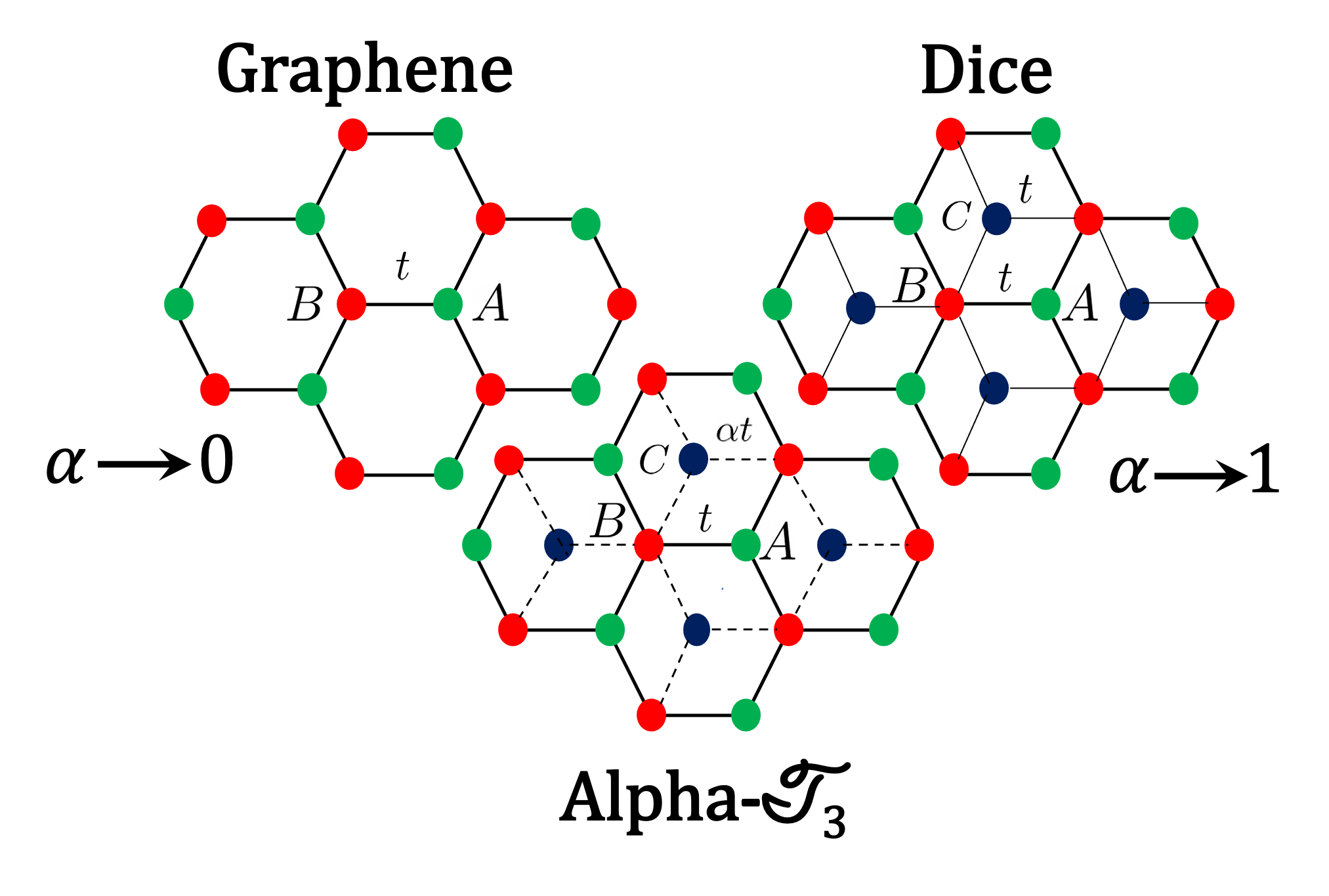
Quantum interference is studied in a three-band model of pseudospin-one fermions in the α − 𝒯 3 𝛼 subscript 𝒯 3 \alpha-\mathcal{T}_{3} α = 0 𝛼 0 \alpha=0 α > 0 𝛼 0 \alpha>0 π 𝜋 \pi α 𝛼 \alpha α = 1 𝛼 1 \alpha=1 α − 𝒯 3 𝛼 subscript 𝒯 3 \alpha-\mathcal{T}_{3}
The interference of waves is so fundamental to physics that it unites various branches, including but not limited to optics, acoustics, quantum mechanics, solids, and cold atoms. In solids, if the disorder is sufficiently high, wave interference can lead to a complete suppression of electronic transport. This phenomenon is known as Anderson localization (AL) [1 ] . A precursor to AL, weak localization (WL) refers to the negative quantum correction to the Drude conductivity due to the interference of electron waves [2 , 3 ] . In WL theory, the deviation to the conductivity is expanded in terms of the parameter λ F / l subscript 𝜆 𝐹 𝑙 \lambda_{F}/l λ F subscript 𝜆 𝐹 \lambda_{F} l 𝑙 l [4 , 5 ] . Coupling the electrons to the magnetic field introduces a finite phase difference between the interfering waves, and hence, magnetoconductivity is a critical tool in the study of WL. In contrast to conventional WL, the presence of spin-orbit coupling can lead to phase shift via spin precession resulting in destructive interference of electron waves, thereby enhancing the conductivity. This phenomenon, termed weak antilocalization [6 ] (WAL), also occurs in Dirac and Weyl materials where pseudospin replaces the actual spin [7 , 8 , 9 , 10 , 11 , 10 , 12 , 12 , 13 , 14 , 15 , 16 , 17 ] .
The Dirac and Weyl equations that originated in particle physics now describe the low-energy physics of materials such as graphene, Weyl semimetals, and Van der Waal structures, leading to their resurgence in condensed matter physics [18 , 19 , 20 ] . The band topology of these materials makes them of high interest, which leads to peculiar properties. For instance, the presence of π 𝜋 \pi [7 , 8 , 9 ] . Recent experimental breakthroughs in Van der Waal heterostructures, such as the discovery of twisted bilayer graphene exhibiting flat bands, have further intensified research in this arena [21 ] .
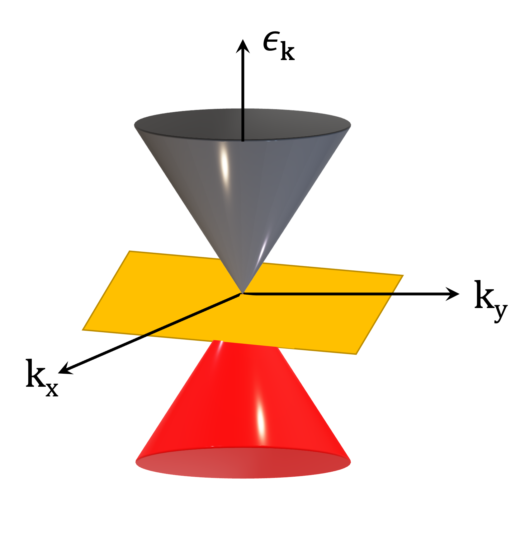
Almost all the quantum interference studies in these materials so far have been typically based on a two-band model that mimics Dirac and Weyl physics. Specifically, it was pointed out in the two-band Dirac fermion that a crossover from weak antilocalization to weak localization occurs as the π 𝜋 \pi [14 ] . The problem of quantum interference effects on localization properties in multi-band models is largely unexplored despite the prevalence of such systems in experiments. For instance, the α − 𝒯 3 𝛼 subscript 𝒯 3 \alpha-\mathcal{T}_{3} [22 ] that synthesizes the Dirac and flat-band physics in a single model comprises a hexagonal lattice with atoms situated at the vertices of the hexagons and their centers, thus describing a three-band system of pseudospin-1 fermions (Fig. 1 α = 0 𝛼 0 \alpha=0 α = 1 𝛼 1 \alpha=1 α − 𝒯 3 𝛼 subscript 𝒯 3 \alpha-\mathcal{T}_{3} 1-x x [23 , 24 , 25 , 26 ] .
In this Letter, we solve the problem of quantum interference in pseudospin-1 fermions and examine the localization properties of electrons in the α − 𝒯 3 𝛼 subscript 𝒯 3 \alpha-\mathcal{T}_{3} α = 0 𝛼 0 \alpha=0 α > 0 𝛼 0 \alpha>0 π 𝜋 \pi α 𝛼 \alpha α = 1 𝛼 1 \alpha=1 α 𝛼 \alpha α − 𝒯 3 𝛼 subscript 𝒯 3 \alpha-\mathcal{T}_{3}
We consider the following model of pseudospin-1 fermions in the α − 𝒯 3 𝛼 subscript 𝒯 3 \alpha-\mathcal{T}_{3} [22 ] :
H μ ( 𝐤 ) = ( 0 a f μ ( 𝐤 ) 0 a f μ ∗ ( 𝐤 ) 0 b f μ ( 𝐤 ) 0 b f μ ∗ ( 𝐤 ) 0 ) superscript 𝐻 𝜇 𝐤 matrix 0 𝑎 subscript 𝑓 𝜇 𝐤 0 𝑎 superscript subscript 𝑓 𝜇 𝐤 0 𝑏 subscript 𝑓 𝜇 𝐤 0 𝑏 subscript superscript 𝑓 𝜇 𝐤 0 H^{\mu}(\mathbf{k})=\begin{pmatrix}0&af_{\mu}(\mathbf{k})&0\\
af_{\mu}^{*}(\mathbf{k})&0&bf_{\mu}(\mathbf{k})\\
0&bf^{*}_{\mu}{(\mathbf{k})}&0\end{pmatrix} (1)
where f μ ( 𝐤 ) = μ ℏ v F ( k x − i k y ) subscript 𝑓 𝜇 𝐤 𝜇 Planck-constant-over-2-pi subscript 𝑣 𝐹 subscript 𝑘 𝑥 𝑖 subscript 𝑘 𝑦 f_{\mu}(\mathbf{k})=\mu\hbar v_{F}(k_{x}-ik_{y}) μ = ± 1 𝜇 plus-or-minus 1 \mu=\pm 1 v F subscript 𝑣 𝐹 v_{F} ψ = tan 1 ( α ) 𝜓 superscript 1 𝛼 \psi=\tan^{1}(\alpha) a = cos ψ 𝑎 𝜓 a=\cos\psi b = sin ψ 𝑏 𝜓 b=\sin\psi ϵ 𝐤 = 0 subscript italic-ϵ 𝐤 0 \epsilon_{\mathbf{k}}=0 + ℏ v F k Planck-constant-over-2-pi subscript 𝑣 𝐹 𝑘 +\hbar v_{F}k − ℏ v F k Planck-constant-over-2-pi subscript 𝑣 𝐹 𝑘 -\hbar v_{F}k 1 ψ 𝐤 ( 𝐫 ) = ( 1 / 2 ) [ μ a e − i μ ϕ , 1 , μ b e i μ ϕ ] e i 𝐤 ⋅ 𝐫 subscript 𝜓 𝐤 𝐫 1 2 𝜇 𝑎 superscript 𝑒 𝑖 𝜇 italic-ϕ 1 𝜇 𝑏 superscript 𝑒 𝑖 𝜇 italic-ϕ
superscript 𝑒 ⋅ 𝑖 𝐤 𝐫 \psi_{\mathbf{k}}(\mathbf{r})=(1/\sqrt{2})[\mu ae^{-i\mu\phi},1,\mu be^{i\mu\phi}]e^{i\mathbf{k}\cdot\mathbf{r}}
We consider both elastic and (pseudo)magnetic impurities such that the impurity potential is given by U ( r ) = U 0 ( r ) + U m ( r ) 𝑈 r subscript 𝑈 0 r subscript 𝑈 𝑚 r U(\textbf{r})=U_{0}(\textbf{r})+U_{m}(\textbf{r}) U 0 ( r ) subscript 𝑈 0 r U_{0}(\textbf{r}) U m ( r ) subscript 𝑈 𝑚 r U_{m}(\textbf{r}) U 0 ( r ) = ∑ R i u 0 i S 0 δ ( r − R i ) subscript 𝑈 0 r subscript subscript R 𝑖 subscript superscript 𝑢 𝑖 0 subscript 𝑆 0 𝛿 r subscript R 𝑖 U_{0}(\textbf{r})=\sum_{\textbf{R}_{i}}u^{i}_{0}S_{0}\delta(\textbf{r}-\textbf{R}_{i}) U m ( r ) = ∑ R i ∑ α = x , y , z u α i S α δ ( r − R i ) subscript 𝑈 𝑚 r subscript subscript R 𝑖 subscript 𝛼 𝑥 𝑦 𝑧
subscript superscript 𝑢 𝑖 𝛼 subscript 𝑆 𝛼 𝛿 r subscript R 𝑖 U_{m}(\textbf{r})=\sum_{\textbf{R}_{i}}\sum\limits_{\alpha=x,y,z}u^{i}_{\alpha}S_{\alpha}\delta(\textbf{r}-\textbf{R}_{i}) R i subscript R 𝑖 \textbf{R}_{i} S 0 ≡ 𝕀 3 subscript 𝑆 0 subscript 𝕀 3 S_{0}\equiv\mathbb{I}_{3} 𝐒 = ( S x , S y , S z ) 𝐒 subscript 𝑆 𝑥 subscript 𝑆 𝑦 subscript 𝑆 𝑧 \mathbf{S}=(S_{x},S_{y},S_{z}) u 0 , α i subscript superscript 𝑢 𝑖 0 𝛼
u^{i}_{0,\alpha} [27 ] . While comparing our results to the particular case of graphene (a → 1 → 𝑎 1 a\rightarrow 1 S i subscript 𝑆 𝑖 S_{i} σ i subscript 𝜎 𝑖 \sigma_{i} a → 1 → 𝑎 1 a\rightarrow 1 C 𝐶 C S z subscript 𝑆 𝑧 S_{z} u z subscript 𝑢 𝑧 u_{z} σ z subscript 𝜎 𝑧 \sigma_{z} u z subscript 𝑢 𝑧 u_{z} − u z subscript 𝑢 𝑧 -u_{z} u x = u y subscript 𝑢 𝑥 subscript 𝑢 𝑦 u_{x}=u_{y} [27 ] , we also present results for the general case.
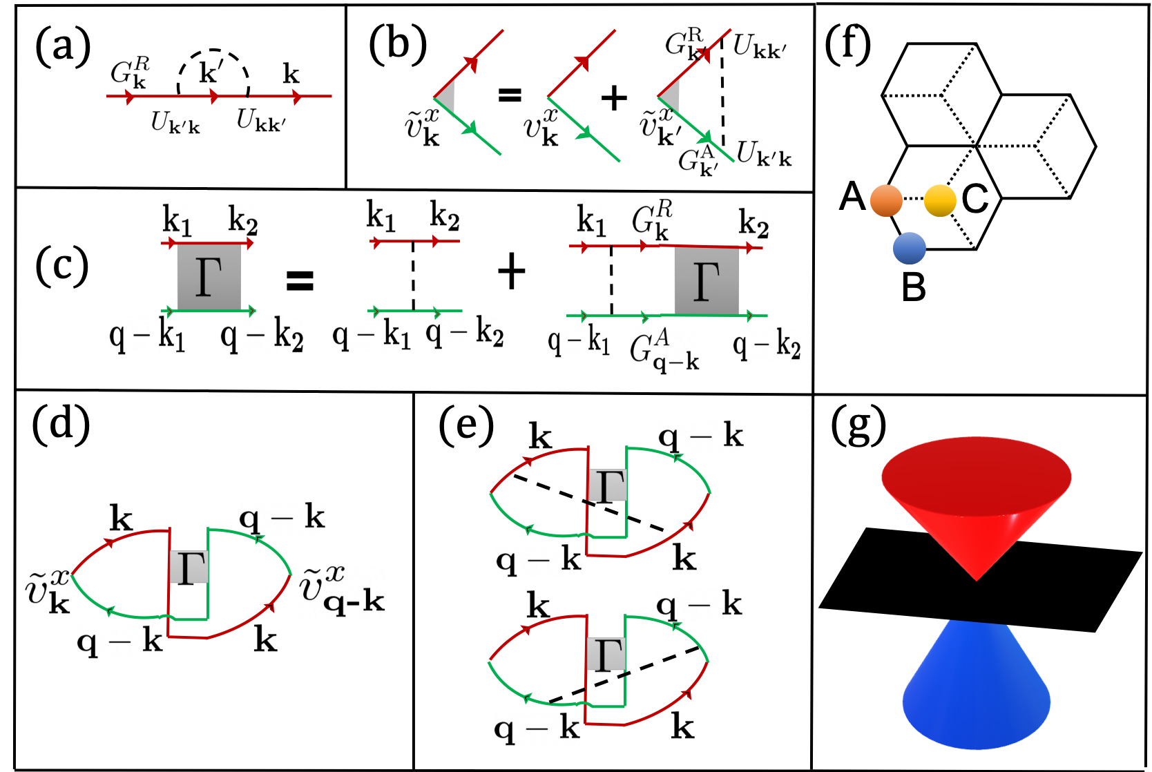
Figure 1: (a) The retarded Green’s function. (b) Vertex correction to the velocity. (c) The bethe-Salpeter equation for the vertex. (d) Bare, and (e) two dressed Hikami boxes for calculation of conductivity. (f) The α − 𝒯 3 𝛼 subscript 𝒯 3 \alpha-\mathcal{T}_{3} A 𝐴 A B 𝐵 B A 𝐴 A C 𝐶 C t 𝑡 t α t 𝛼 𝑡 \alpha t α − 𝒯 3 𝛼 subscript 𝒯 3 \alpha-\mathcal{T}_{3}
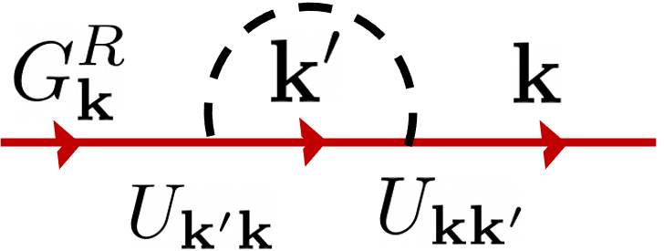
Quantum interference to conductivity in pseudospin-1 fermions is calculated diagrammatically (see Fig. 1 G k R / A ( ω ) = 1 / ( ω − ϵ k ± i ℏ / 2 τ ) subscript superscript 𝐺 𝑅 𝐴 k 𝜔 1 plus-or-minus 𝜔 subscript italic-ϵ k 𝑖 Planck-constant-over-2-pi 2 𝜏 G^{R/A}_{\textbf{k}}(\omega)={1}/{(\omega-\epsilon_{\textbf{k}}\pm i{\hbar}/{2\tau})} τ − 1 = τ e − 1 + τ z − 1 + 2 τ x − 1 superscript 𝜏 1 superscript subscript 𝜏 𝑒 1 superscript subscript 𝜏 𝑧 1 2 superscript subscript 𝜏 𝑥 1 \tau^{-1}=\tau_{e}^{-1}+\tau_{z}^{-1}+2\tau_{x}^{-1} ℏ τ e − 1 = 2 π N F n 0 u 0 2 ( a 4 + b 4 + 1 ) / 4 Planck-constant-over-2-pi subscript superscript 𝜏 1 𝑒 2 𝜋 subscript 𝑁 𝐹 subscript 𝑛 0 subscript superscript 𝑢 2 0 superscript 𝑎 4 superscript 𝑏 4 1 4 {\hbar}{\tau}^{-1}_{e}={2\pi N_{F}}{n_{0}u^{2}_{0}}(a^{4}+b^{4}+1)/4 ℏ τ x − 1 = 2 π N F n m u x 2 / 2 Planck-constant-over-2-pi superscript subscript 𝜏 𝑥 1 2 𝜋 subscript 𝑁 𝐹 subscript 𝑛 𝑚 subscript superscript 𝑢 2 𝑥 2 {\hbar}{\tau_{x}^{-1}}={2\pi N_{F}}{n_{m}u^{2}_{x}}/{2} ℏ τ z − 1 = 2 π N F n m u z 2 ( a 4 + b 4 ) / 4 Planck-constant-over-2-pi superscript subscript 𝜏 𝑧 1 2 𝜋 subscript 𝑁 𝐹 subscript 𝑛 𝑚 subscript superscript 𝑢 2 𝑧 superscript 𝑎 4 superscript 𝑏 4 4 {\hbar}{\tau_{z}^{-1}}={2\pi N_{F}}{n_{m}u^{2}_{z}}(a^{4}+b^{4})/{4} τ e subscript 𝜏 𝑒 \tau_{e} ℓ e subscript ℓ 𝑒 \ell_{e} ℓ e = D τ e subscript ℓ 𝑒 𝐷 subscript 𝜏 𝑒 \ell_{e}=\sqrt{D\tau_{e}} D = v F 2 τ / 2 𝐷 superscript subscript 𝑣 𝐹 2 𝜏 2 D=v_{F}^{2}\tau/2 l x subscript 𝑙 𝑥 l_{x} l z subscript 𝑙 𝑧 l_{z} 1 v ~ 𝐤 i = v 𝐤 i + ∑ 𝐤 ′ G 𝐤 ′ R G 𝐤 ′ A ⟨ U 𝐤 , 𝐤 ′ U 𝐤 ′ , 𝐤 ⟩ imp v ~ 𝐤 ′ i superscript subscript ~ 𝑣 𝐤 𝑖 superscript subscript 𝑣 𝐤 𝑖 subscript superscript 𝐤 ′ superscript subscript 𝐺 superscript 𝐤 ′ R superscript subscript 𝐺 superscript 𝐤 ′ A subscript delimited-⟨⟩ subscript 𝑈 𝐤 superscript 𝐤 ′
subscript 𝑈 superscript 𝐤 ′ 𝐤
imp superscript subscript ~ 𝑣 superscript 𝐤 ′ 𝑖 \tilde{v}_{\mathbf{k}}^{i}=v_{\mathbf{k}}^{i}+\sum_{\mathbf{k}^{\prime}}G_{\mathbf{k}^{\prime}}^{\mathrm{R}}G_{\mathbf{k}^{\prime}}^{\mathrm{A}}\left\langle U_{\mathbf{k},\mathbf{k}^{\prime}}U_{\mathbf{k}^{\prime},\mathbf{k}}\right\rangle_{\textrm{imp}}\tilde{v}_{\mathbf{k}^{\prime}}^{i} v ~ 𝐤 i = η ν v 𝐤 superscript subscript ~ 𝑣 𝐤 𝑖 subscript 𝜂 𝜈 subscript 𝑣 𝐤 \tilde{v}_{\mathbf{k}}^{i}=\eta_{\nu}v_{\mathbf{k}} η ν subscript 𝜂 𝜈 \eta_{\nu} [27 ]
η v − 1 = 1 − ( α e / ( a 4 + b 4 + 1 ) + 2 a b α x ) . subscript superscript 𝜂 1 𝑣 1 subscript 𝛼 𝑒 superscript 𝑎 4 superscript 𝑏 4 1 2 𝑎 𝑏 subscript 𝛼 𝑥 \displaystyle\eta^{-1}_{v}={1-\left({\alpha_{e}}/{(a^{4}+b^{4}+1)}+2ab{\alpha_{x}}\right)}. (2)
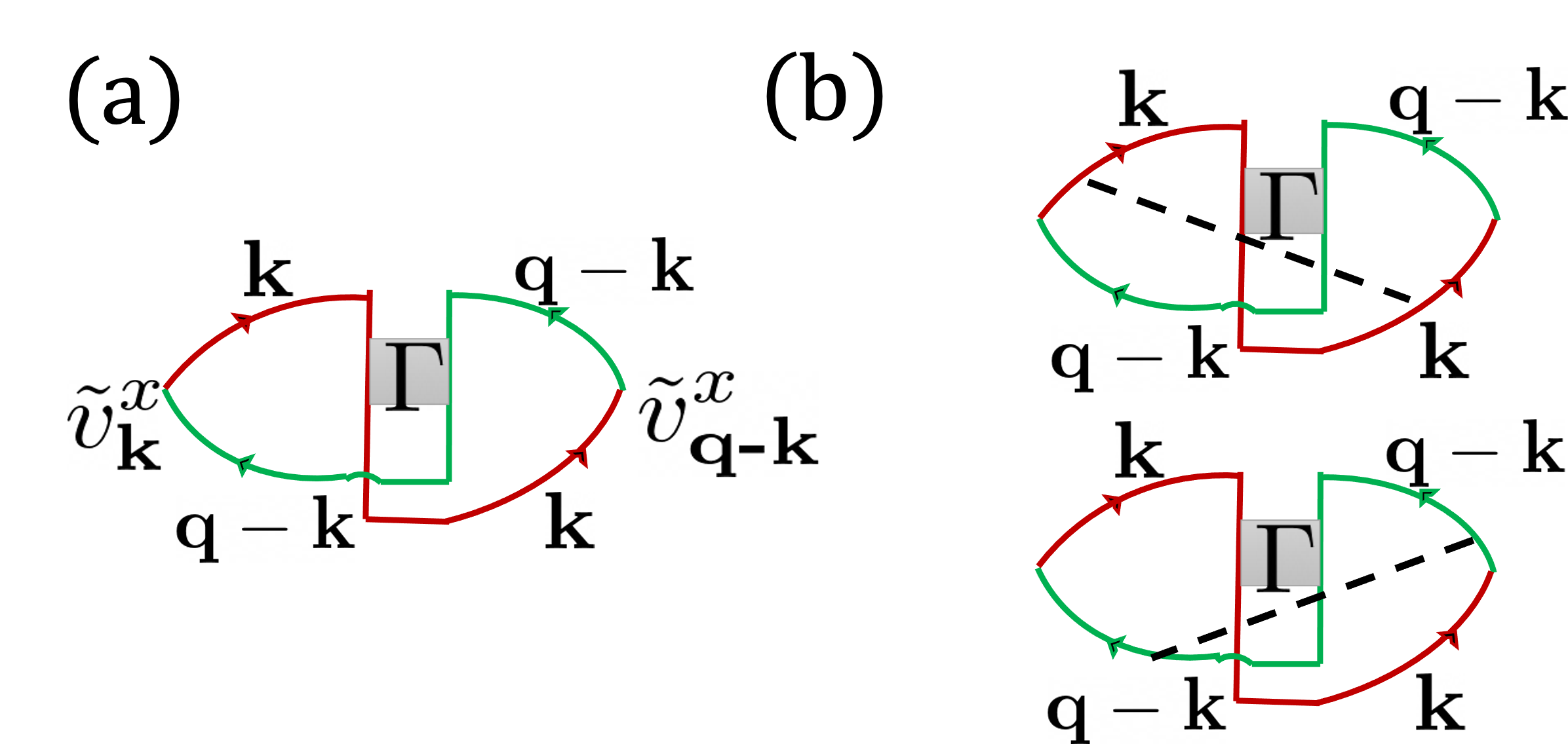
We recover η ν = 2 subscript 𝜂 𝜈 2 \eta_{\nu}=2 [7 , 9 ] . The net conductivity is evaluated by summing over the contribution of one bare and two dressed Hikami boxes (Fig. 1 [27 ] :
σ = − e 2 N F τ 3 η v 2 v F 2 ℏ 2 ( 1 + 2 η H ) ∑ q Γ ( q ) , 𝜎 superscript 𝑒 2 subscript 𝑁 𝐹 superscript 𝜏 3 subscript superscript 𝜂 2 𝑣 subscript superscript 𝑣 2 𝐹 superscript Planck-constant-over-2-pi 2 1 2 subscript 𝜂 𝐻 subscript q Γ q \displaystyle\sigma=-\frac{e^{2}N_{F}\tau^{3}\eta^{2}_{v}v^{2}_{F}}{\hbar^{2}}(1+2\eta_{H})\sum_{\textbf{q}}\Gamma(\textbf{q}), (3)
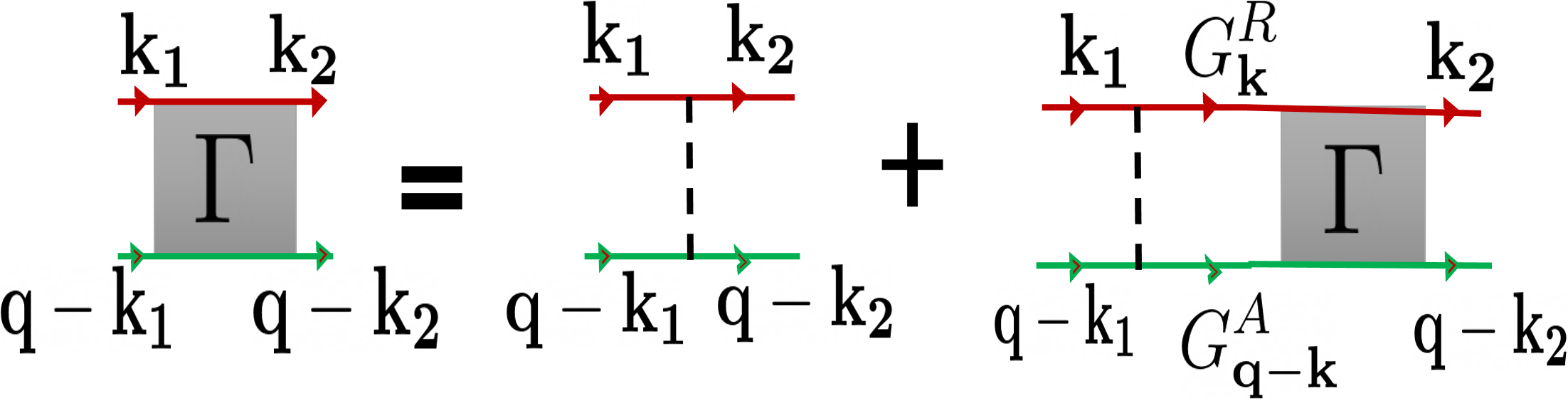
where N F = E F / 2 π ( ℏ v F ) 2 subscript 𝑁 𝐹 subscript 𝐸 𝐹 2 𝜋 superscript Planck-constant-over-2-pi subscript 𝑣 𝐹 2 N_{F}={E_{F}}/{2\pi(\hbar v_{F})^{2}} η H = − ( 1 / 2 ) ( 1 − η v − 1 ) subscript 𝜂 𝐻 1 2 1 subscript superscript 𝜂 1 𝑣 \eta_{H}=-({1}/{2})\left(1-\eta^{-1}_{v}\right) Γ ( 𝐪 ) Γ 𝐪 \Gamma(\mathbf{q}) Γ 𝐤 1 , 𝐤 2 = Γ 𝐤 1 , 𝐤 2 0 + ∑ 𝐤 Γ 𝐤 1 , 𝐤 0 G 𝐤 R G 𝐪 − 𝐤 A Γ 𝐤 , 𝐤 2 subscript Γ subscript 𝐤 1 subscript 𝐤 2
superscript subscript Γ subscript 𝐤 1 subscript 𝐤 2
0 subscript 𝐤 superscript subscript Γ subscript 𝐤 1 𝐤
0 superscript subscript 𝐺 𝐤 𝑅 superscript subscript 𝐺 𝐪 𝐤 𝐴 subscript Γ 𝐤 subscript 𝐤 2
\Gamma_{\mathbf{k}_{1},\mathbf{k}_{2}}=\Gamma_{\mathbf{k}_{1},\mathbf{k}_{2}}^{0}+\sum_{\mathbf{k}}\Gamma_{\mathbf{k}_{1},\mathbf{k}}^{0}G_{\mathbf{k}}^{R}G_{\mathbf{q}-\mathbf{k}}^{A}\Gamma_{\mathbf{k},\mathbf{k}_{2}} 𝐪 = 𝐤 1 + 𝐤 2 𝐪 subscript 𝐤 1 subscript 𝐤 2 \mathbf{q}=\mathbf{k}_{1}+\mathbf{k}_{2} η H = − 1 / 4 subscript 𝜂 𝐻 1 4 \eta_{H}=-1/4 𝐪 → 0 → 𝐪 0 \mathbf{q}\rightarrow 0 Γ 𝐤 𝟏 , 𝐤 𝟐 0 ≡ ⟨ U 𝐤 𝟏 , 𝐤 2 U − 𝐤 𝟏 , − 𝐤 𝟐 ⟩ imp = ( ℏ / 2 π N F τ ) ∑ m ∑ n z m n e i m ϕ 1 e i n ϕ 2 \Gamma^{0}_{\mathbf{k_{1},k_{2}}}\equiv\langle U_{\mathbf{k_{1}},\mathbf{k}_{2}}U_{\mathbf{-k_{1}},\mathbf{-k_{2}}}\bigl{\rangle}_{\mathrm{imp}}=({\hbar}/{2\pi N_{F}\tau})\sum_{m}\sum_{n}z_{mn}e^{im\phi_{1}}e^{in\phi_{2}} m 𝑚 m n 𝑛 n z m n subscript 𝑧 𝑚 𝑛 z_{mn} z 𝑧 z [27 ]
z = ( 0 0 0 0 z ( − 22 ) 0 0 0 z ( − 11 ) 0 0 0 z ( 00 ) 0 0 0 z ( 1 − 1 ) 0 0 0 z ( 2 − 2 ) 0 0 0 0 ) , 𝑧 matrix 0 0 0 0 superscript 𝑧 22 0 0 0 superscript 𝑧 11 0 0 0 superscript 𝑧 00 0 0 0 superscript 𝑧 1 1 0 0 0 superscript 𝑧 2 2 0 0 0 0 missing-subexpression \displaystyle z=\begin{pmatrix}0&0&0&0&z^{(-22)}\\
0&0&0&z^{(-11)}&0\\
0&0&z^{(00)}&0&0\\
0&z^{(1-1)}&0&0&0\\
z^{(2-2)}&0&0&0&0&\end{pmatrix}, (4)
and the elements are given by z ( − 22 ) = b 4 α e a 4 + b 4 + 1 + b 4 α z a 4 + b 4 superscript 𝑧 22 superscript 𝑏 4 subscript 𝛼 𝑒 superscript 𝑎 4 superscript 𝑏 4 1 superscript 𝑏 4 subscript 𝛼 𝑧 superscript 𝑎 4 superscript 𝑏 4 z^{(-22)}=\frac{b^{4}\alpha_{e}}{a^{4}+b^{4}+1}+\frac{b^{4}\alpha_{z}}{a^{4}+b^{4}} z ( − 11 ) = 2 b 2 α e a 4 + b 4 + 1 − 2 b 2 α x superscript 𝑧 11 2 superscript 𝑏 2 subscript 𝛼 𝑒 superscript 𝑎 4 superscript 𝑏 4 1 2 superscript 𝑏 2 subscript 𝛼 𝑥 z^{(-11)}=\frac{2b^{2}\alpha_{e}}{a^{4}+b^{4}+1}-2b^{2}\alpha_{x} z ( 00 ) = ( 2 a 2 b 2 + 1 ) α e a 4 + b 4 + 1 − 2 a 2 b 2 α z a 4 + b 4 − 4 a b α x superscript 𝑧 00 2 superscript 𝑎 2 superscript 𝑏 2 1 subscript 𝛼 𝑒 superscript 𝑎 4 superscript 𝑏 4 1 2 superscript 𝑎 2 superscript 𝑏 2 subscript 𝛼 𝑧 superscript 𝑎 4 superscript 𝑏 4 4 𝑎 𝑏 subscript 𝛼 𝑥 z^{(00)}=\frac{\left(2a^{2}b^{2}+1\right)\alpha_{e}}{a^{4}+b^{4}+1}-\frac{2a^{2}b^{2}\alpha_{z}}{a^{4}+b^{4}}-4ab\alpha_{x} z ( 1 − 1 ) = 2 a 2 α e a 4 + b 4 + 1 − 2 a 2 α x superscript 𝑧 1 1 2 superscript 𝑎 2 subscript 𝛼 𝑒 superscript 𝑎 4 superscript 𝑏 4 1 2 superscript 𝑎 2 subscript 𝛼 𝑥 z^{(1-1)}=\frac{2a^{2}\alpha_{e}}{a^{4}+b^{4}+1}-2a^{2}\alpha_{x} z ( 2 − 2 ) = a 4 α e a 4 + b 4 + 1 + a 4 α z a 4 + b 4 superscript 𝑧 2 2 superscript 𝑎 4 subscript 𝛼 𝑒 superscript 𝑎 4 superscript 𝑏 4 1 superscript 𝑎 4 subscript 𝛼 𝑧 superscript 𝑎 4 superscript 𝑏 4 z^{(2-2)}=\frac{a^{4}\alpha_{e}}{a^{4}+b^{4}+1}+\frac{a^{4}\alpha_{z}}{a^{4}+b^{4}}
The Bethe-Salpeter equation (Fig. 1 Γ 𝐤 𝟏 , 𝐤 𝟐 = ( ℏ / 2 π N F τ ) ∑ m ∑ n = γ m n e i m ϕ 1 e i n ϕ 2 subscript Γ subscript 𝐤 1 subscript 𝐤 2
Planck-constant-over-2-pi 2 𝜋 subscript 𝑁 𝐹 𝜏 subscript 𝑚 subscript 𝑛 superscript 𝛾 𝑚 𝑛 superscript 𝑒 𝑖 𝑚 subscript italic-ϕ 1 superscript 𝑒 𝑖 𝑛 subscript italic-ϕ 2 \Gamma_{\mathbf{k_{1},k_{2}}}=({\hbar}/{2\pi N_{F}\tau})\sum_{m}\sum_{n}=\gamma^{mn}e^{im\phi_{1}}e^{in\phi_{2}} γ m n superscript 𝛾 𝑚 𝑛 \gamma^{mn} γ 𝛾 \gamma γ = ( I − z Φ ) − 1 z 𝛾 superscript 𝐼 𝑧 Φ 1 𝑧 \gamma=(I-z\Phi)^{-1}z Φ m n = 1 2 π ∫ 0 2 π e i ( m + n ) ϕ ( 1 + i τ 𝐪 ⋅ 𝐯 F ) − 1 𝑑 ϕ superscript Φ 𝑚 𝑛 1 2 𝜋 superscript subscript 0 2 𝜋 superscript 𝑒 𝑖 𝑚 𝑛 italic-ϕ superscript 1 ⋅ 𝑖 𝜏 𝐪 subscript 𝐯 𝐹 1 differential-d italic-ϕ \Phi^{mn}=\frac{1}{2\pi}\int_{0}^{2\pi}{e^{i(m+n)\phi}}({1+i\tau\mathbf{q}\cdot\mathbf{v}_{F}})^{-1}d\phi [27 ]
γ ( − m m ) = superscript 𝛾 𝑚 𝑚 absent \displaystyle{\gamma^{(-mm)}}=
2 ∏ p ≠ m g ( − p p ) ∏ k ( g ( − k k ) + Q 2 ( ∑ l 1 g ( − l l ) + ∑ q 1 g ( − q q ) g ( − q − 1 , q + 1 ) ) ) , 2 subscript product 𝑝 𝑚 superscript 𝑔 𝑝 𝑝 subscript product 𝑘 superscript 𝑔 𝑘 𝑘 superscript 𝑄 2 subscript 𝑙 1 superscript 𝑔 𝑙 𝑙 subscript 𝑞 1 superscript 𝑔 𝑞 𝑞 superscript 𝑔 𝑞 1 𝑞 1 \displaystyle\frac{2\prod\limits_{p\neq m}g^{(-pp)}}{\prod\limits_{k}\left(g^{(-kk)}+Q^{2}\left(\sum\limits_{l}\frac{1}{g^{(-ll)}}+\sum\limits_{q}\frac{1}{g^{(-qq)}g^{(-q-1,q+1)}}\right)\right)}, (5)
where the “Cooperon gaps” have been introduced g ( − i i ) = 2 ( 1 − z ( − i i ) ) / z ( − i i ) superscript 𝑔 𝑖 𝑖 2 1 superscript 𝑧 𝑖 𝑖 superscript 𝑧 𝑖 𝑖 g^{(-ii)}=2(1-z^{(-ii)})/z^{(-ii)} Q = q v F τ 𝑄 𝑞 subscript 𝑣 𝐹 𝜏 Q=qv_{F}\tau 5 3 Γ ( 𝐪 ) Γ 𝐪 \Gamma(\mathbf{q}) [27 ] .
The conductivity is evaluated by integrating Eq. 3 1 / l e 1 subscript 𝑙 𝑒 1/l_{e} 1 / l ϕ 1 subscript 𝑙 italic-ϕ 1/l_{\phi} [7 ] . In the presence of a magnetic field, the wavevector q 𝑞 q q n 2 = ( n + 1 / 2 ) 4 e B / ℏ superscript subscript 𝑞 𝑛 2 𝑛 1 2 4 𝑒 𝐵 Planck-constant-over-2-pi q_{n}^{2}=(n+1/2)4eB/\hbar n 𝑛 n n 𝑛 n Δ σ ( B ) Δ 𝜎 𝐵 \Delta\sigma(B) [3 ] . We present magnetoconductivity results focusing on the weak-B 𝐵 B l B 2 ≫ l e 2 much-greater-than superscript subscript 𝑙 𝐵 2 superscript subscript 𝑙 𝑒 2 l_{B}^{2}\gg l_{e}^{2}
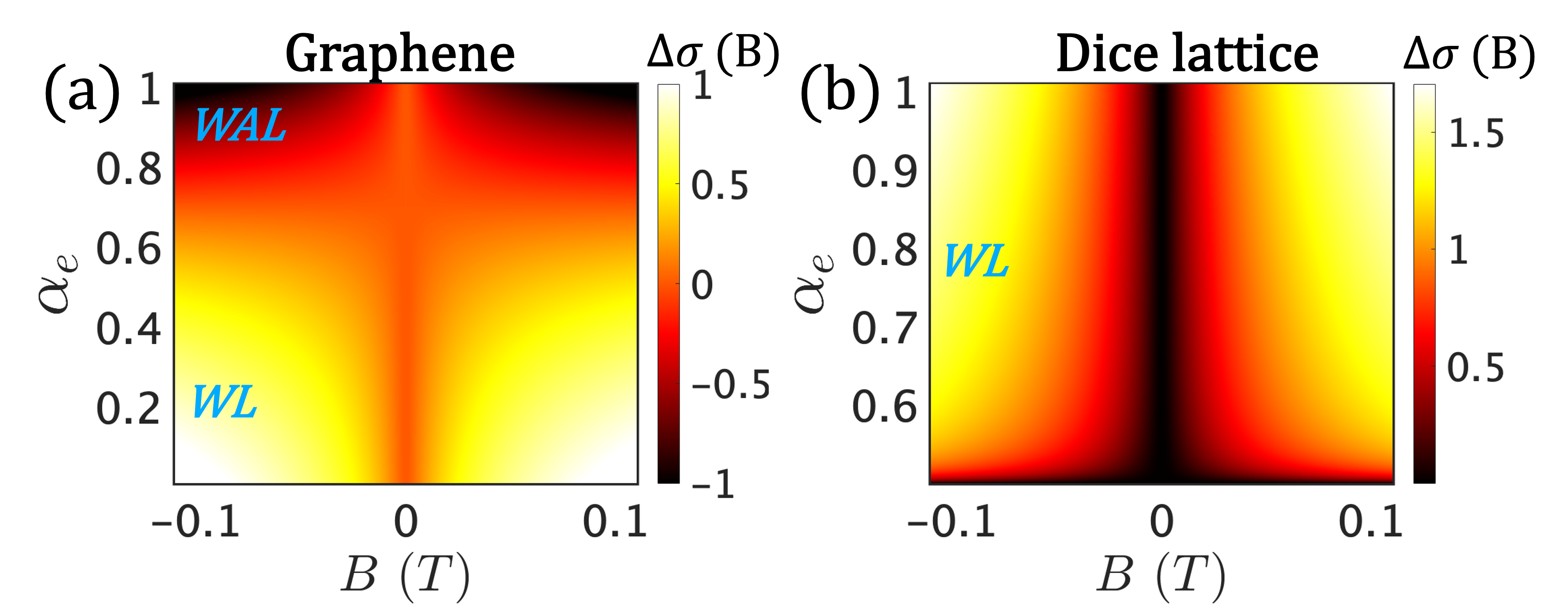
Figure 2: Magnetoconductivity in the units of e 2 / π ℏ superscript 𝑒 2 𝜋 Planck-constant-over-2-pi e^{2}/\pi\hbar α e subscript 𝛼 𝑒 \alpha_{e} l ϕ = 300 subscript 𝑙 italic-ϕ 300 l_{\phi}=300 l e = 1000 subscript 𝑙 𝑒 1000 l_{e}=1000
In the case of graphene (a = 1 𝑎 1 a=1 g ( 1 − 1 ) superscript 𝑔 1 1 g^{(1-1)} g ( 2 − 2 ) superscript 𝑔 2 2 g^{(2-2)} [27 ]
Δ σ ( B ) = Δ 𝜎 𝐵 absent \displaystyle\Delta\sigma(B)=
e 2 π h ∑ i = 0 , 1 α i [ Ψ ( ℓ B 2 ℓ ϕ 2 + ℓ B 2 ℓ i 2 + 1 2 ) − ln ( ℓ B 2 ℓ ϕ 2 + ℓ B 2 ℓ i 2 ) ] , superscript 𝑒 2 𝜋 ℎ subscript 𝑖 0 1
subscript 𝛼 𝑖 delimited-[] Ψ subscript superscript ℓ 2 𝐵 subscript superscript ℓ 2 italic-ϕ subscript superscript ℓ 2 𝐵 subscript superscript ℓ 2 𝑖 1 2 subscript superscript ℓ 2 𝐵 subscript superscript ℓ 2 italic-ϕ subscript superscript ℓ 2 𝐵 subscript superscript ℓ 2 𝑖 \displaystyle\frac{e^{2}}{\pi h}\sum_{i=0,1}\alpha_{i}\left[\Psi\left(\frac{\ell^{2}_{B}}{\ell^{2}_{\phi}}+\frac{\ell^{2}_{B}}{\ell^{2}_{i}}+\frac{1}{2}\right)-\ln\left(\frac{\ell^{2}_{B}}{\ell^{2}_{\phi}}+\frac{\ell^{2}_{B}}{\ell^{2}_{i}}\right)\right], (6)
where Ψ Ψ \Psi
α 0 = η v 2 ( 1 + 2 η H ) 2 ( 1 + 1 g ( 1 − 1 ) ) , α 1 = − η v 2 ( 1 + 2 η H ) 2 ( 1 g ( 2 − 2 ) + 1 g ( 00 ) + 1 ) , formulae-sequence subscript 𝛼 0 subscript superscript 𝜂 2 𝑣 1 2 subscript 𝜂 𝐻 2 1 1 superscript 𝑔 1 1 subscript 𝛼 1 subscript superscript 𝜂 2 𝑣 1 2 subscript 𝜂 𝐻 2 1 superscript 𝑔 2 2 1 superscript 𝑔 00 1 \displaystyle\alpha_{0}=\frac{\eta^{2}_{v}(1+2\eta_{H})}{2\left(1+\frac{1}{g^{(1-1)}}\right)},\quad\alpha_{1}=-\frac{\eta^{2}_{v}(1+2\eta_{H})}{2\left(\frac{1}{g^{(2-2)}}+\frac{1}{g^{(00)}}+1\right)},
ℓ 0 − 2 = g ( 2 − 2 ) 2 ℓ 2 ( 1 + 1 g ( 1 − 1 ) ) , ℓ 1 − 2 = g ( 1 − 1 ) 2 ℓ 2 ( 1 g ( 2 − 2 ) + 1 g ( 00 ) + 1 ) , formulae-sequence superscript subscript ℓ 0 2 superscript 𝑔 2 2 2 superscript ℓ 2 1 1 superscript 𝑔 1 1 subscript superscript ℓ 2 1 superscript 𝑔 1 1 2 superscript ℓ 2 1 superscript 𝑔 2 2 1 superscript 𝑔 00 1 \displaystyle{\ell_{0}}^{-2}=\frac{g^{(2-2)}}{2\ell^{2}\left(1+\frac{1}{g^{(1-1)}}\right)},\quad\ell^{-2}_{1}=\frac{g^{(1-1)}}{2\ell^{2}\left(\frac{1}{g^{(2-2)}}+\frac{1}{g^{(00)}}+1\right)}, (7)
where l − 2 = l e − 2 + l z − 2 + 2 l x − 2 superscript 𝑙 2 superscript subscript 𝑙 𝑒 2 superscript subscript 𝑙 𝑧 2 2 superscript subscript 𝑙 𝑥 2 l^{-2}=l_{e}^{-2}+l_{z}^{-2}+2l_{x}^{-2} α e subscript 𝛼 𝑒 \alpha_{e} [14 ] . We plot this behavior in Fig. 2 a = 0 𝑎 0 a=0 g ( − 11 ) superscript 𝑔 11 g^{(-11)} g ( − 22 ) superscript 𝑔 22 g^{(-22)}
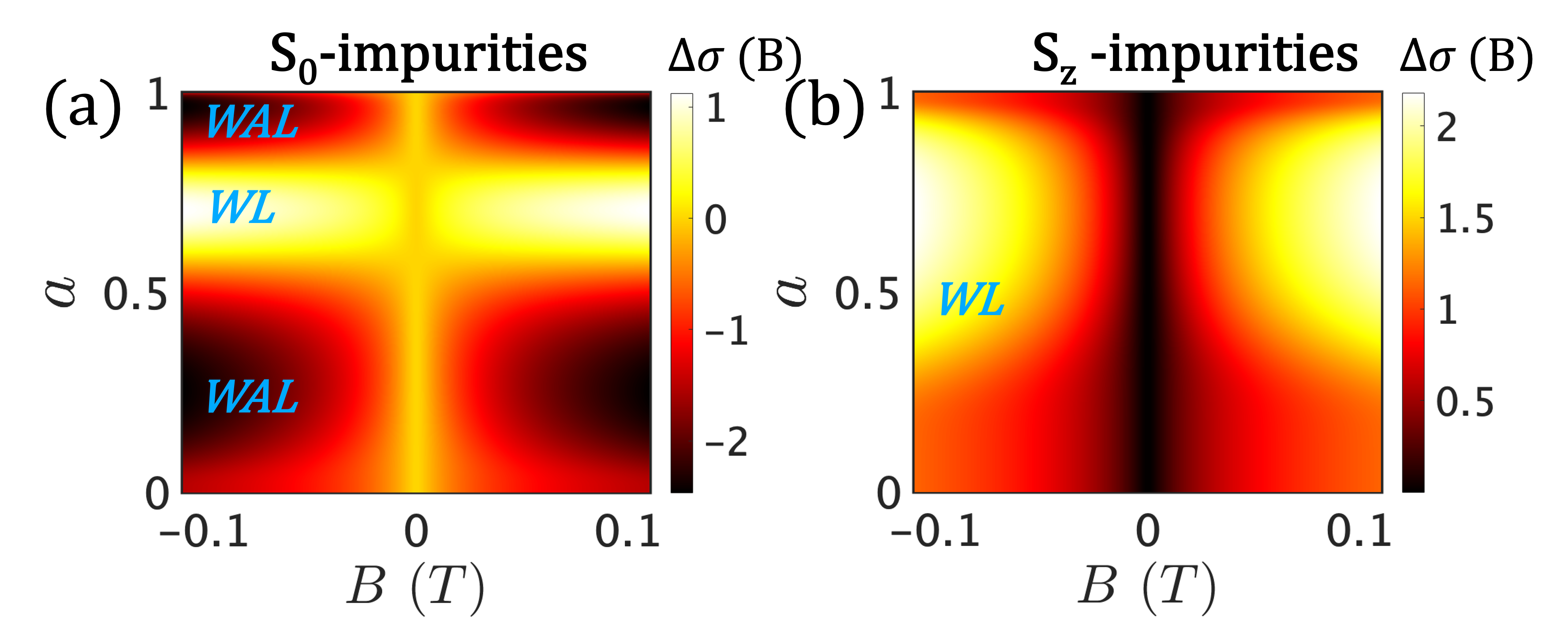
Figure 3: Magnetoconductivity in the units of e 2 / π ℏ superscript 𝑒 2 𝜋 Planck-constant-over-2-pi e^{2}/\pi\hbar a = 0 𝑎 0 a=0 a = 2 − 1 2 𝑎 superscript 2 1 2 a=2^{-\frac{1}{2}} a = 1 𝑎 1 a=1 α e = 1 subscript 𝛼 𝑒 1 \alpha_{e}=1 S z subscript 𝑆 𝑧 S_{z} l ϕ = 300 subscript 𝑙 italic-ϕ 300 l_{\phi}=300 l e = l z = 1000 subscript 𝑙 𝑒 subscript 𝑙 𝑧 1000 l_{e}=l_{z}=1000
In the case of dice lattice (a = 2 − 1 2 𝑎 superscript 2 1 2 a=2^{-\frac{1}{2}} g ( 00 ) superscript 𝑔 00 g^{(00)} [27 ]
Δ σ ( B ) = Δ 𝜎 𝐵 absent \displaystyle\Delta\sigma(B)=
e 2 π h α 0 [ Ψ ( ℓ B 2 ℓ ϕ 2 + ℓ B 2 ℓ i 2 + 1 2 ) − ln ( ℓ B 2 ℓ ϕ 2 + ℓ B 2 ℓ i 2 ) ] , superscript 𝑒 2 𝜋 ℎ subscript 𝛼 0 delimited-[] Ψ subscript superscript ℓ 2 𝐵 subscript superscript ℓ 2 italic-ϕ subscript superscript ℓ 2 𝐵 subscript superscript ℓ 2 𝑖 1 2 subscript superscript ℓ 2 𝐵 subscript superscript ℓ 2 italic-ϕ subscript superscript ℓ 2 𝐵 subscript superscript ℓ 2 𝑖 \displaystyle\frac{e^{2}}{\pi h}\alpha_{0}\left[\Psi\left(\frac{\ell^{2}_{B}}{\ell^{2}_{\phi}}+\frac{\ell^{2}_{B}}{\ell^{2}_{i}}+\frac{1}{2}\right)-\ln\left(\frac{\ell^{2}_{B}}{\ell^{2}_{\phi}}+\frac{\ell^{2}_{B}}{\ell^{2}_{i}}\right)\right], (8)
where
α 0 = η v 2 ( 1 + 2 η H ) 2 ( 1 + 1 g ( − 11 ) ) , ℓ 0 − 2 = g ( 00 ) 2 ℓ 2 ( 1 + 1 g ( − 11 ) ) , formulae-sequence subscript 𝛼 0 subscript superscript 𝜂 2 𝑣 1 2 subscript 𝜂 𝐻 2 1 1 superscript 𝑔 11 subscript superscript ℓ 2 0 superscript 𝑔 00 2 superscript ℓ 2 1 1 superscript 𝑔 11 \displaystyle\alpha_{0}=\frac{\eta^{2}_{v}(1+2\eta_{H})}{2\left(1+\frac{1}{g^{(-11)}}\right)},\quad\ell^{-2}_{0}=\frac{g^{(00)}}{2\ell^{2}\left(1+\frac{1}{g^{(-11)}}\right)}, (9)
In contrast to graphene lattice, dice lattice displays only weak localization, as seen in Fig. 2 π 𝜋 \pi a = 1 𝑎 1 a=1 a = 2 − 1 2 𝑎 superscript 2 1 2 a=2^{-\frac{1}{2}}
In the presence of only elastic impurities (α e = 1 subscript 𝛼 𝑒 1 \alpha_{e}=1 g ( 1 − 1 ) superscript 𝑔 1 1 g^{(1-1)} g ( − 11 ) superscript 𝑔 11 g^{(-11)} g ( 00 ) superscript 𝑔 00 g^{(00)} [27 ]
Δ σ ( B ) = Δ 𝜎 𝐵 absent \displaystyle\Delta\sigma(B)=
e 2 π h ∑ i = 0 , 1 , 2 α i [ Ψ ( ℓ B 2 ℓ ϕ 2 + ℓ B 2 ℓ i 2 + 1 2 ) − ln ( ℓ B 2 ℓ ϕ 2 + ℓ B 2 ℓ i 2 ) ] , superscript 𝑒 2 𝜋 ℎ subscript 𝑖 0 1 2
subscript 𝛼 𝑖 delimited-[] Ψ subscript superscript ℓ 2 𝐵 subscript superscript ℓ 2 italic-ϕ subscript superscript ℓ 2 𝐵 subscript superscript ℓ 2 𝑖 1 2 subscript superscript ℓ 2 𝐵 subscript superscript ℓ 2 italic-ϕ subscript superscript ℓ 2 𝐵 subscript superscript ℓ 2 𝑖 \displaystyle\frac{e^{2}}{\pi h}\sum_{i=0,1,2}\alpha_{i}\left[\Psi\left(\frac{\ell^{2}_{B}}{\ell^{2}_{\phi}}+\frac{\ell^{2}_{B}}{\ell^{2}_{i}}+\frac{1}{2}\right)-\ln\left(\frac{\ell^{2}_{B}}{\ell^{2}_{\phi}}+\frac{\ell^{2}_{B}}{\ell^{2}_{i}}\right)\right], (10)
where
α 0 = − η v 2 ( 1 + 2 η H ) 2 ( 1 + 1 g ( 00 ) ) , ℓ 0 − 2 = g ( 1 − 1 ) 2 l 2 ( 1 + 1 g ( 00 ) ) , formulae-sequence subscript 𝛼 0 subscript superscript 𝜂 2 𝑣 1 2 subscript 𝜂 𝐻 2 1 1 superscript 𝑔 00 subscript superscript ℓ 2 0 superscript 𝑔 1 1 2 superscript 𝑙 2 1 1 superscript 𝑔 00 \displaystyle\alpha_{0}=-\frac{\eta^{2}_{v}(1+2\eta_{H})}{2\left(1+\frac{1}{g^{(00)}}\right)},\quad\ell^{-2}_{0}=\frac{g^{(1-1)}}{2l^{2}\left(1+\frac{1}{g^{(00)}}\right)},
α 1 = η v 2 ( 1 + 2 η H ) 2 ( 1 g ( 1 − 1 ) + 1 g ( − 11 ) + 1 ) , ℓ 1 − 2 = g ( 00 ) 2 l 2 ( 1 g ( 1 − 1 ) + 1 g ( − 11 ) + 1 ) , formulae-sequence subscript 𝛼 1 subscript superscript 𝜂 2 𝑣 1 2 subscript 𝜂 𝐻 2 1 superscript 𝑔 1 1 1 superscript 𝑔 11 1 subscript superscript ℓ 2 1 superscript 𝑔 00 2 superscript 𝑙 2 1 superscript 𝑔 1 1 1 superscript 𝑔 11 1 \displaystyle\alpha_{1}=\frac{\eta^{2}_{v}(1+2\eta_{H})}{2\left(\frac{1}{g^{(1-1)}}+\frac{1}{g^{(-11)}}+1\right)},\ell^{-2}_{1}=\frac{g^{(00)}}{2l^{2}\left(\frac{1}{g^{(1-1)}}+\frac{1}{g^{(-11)}}+1\right)},
α 2 = − η v 2 ( 1 + 2 η H ) 2 ( 1 + 1 g ( 00 ) ) , ℓ 2 − 2 = g ( − 11 ) 2 l 2 ( 1 + 1 g ( 00 ) ) formulae-sequence subscript 𝛼 2 subscript superscript 𝜂 2 𝑣 1 2 subscript 𝜂 𝐻 2 1 1 superscript 𝑔 00 subscript superscript ℓ 2 2 superscript 𝑔 11 2 superscript 𝑙 2 1 1 superscript 𝑔 00 \displaystyle\alpha_{2}=-\frac{\eta^{2}_{v}(1+2\eta_{H})}{2\left(1+\frac{1}{g^{(00)}}\right)},\quad\ell^{-2}_{2}=\frac{g^{(-11)}}{2l^{2}\left(1+\frac{1}{g^{(00)}}\right)} (11)
In Fig. 3 a 𝑎 a a = 0 𝑎 0 a=0 a 𝑎 a π 𝜋 \pi a = 0 𝑎 0 a=0 a 𝑎 a 2 − 1 2 superscript 2 1 2 2^{-\frac{1}{2}} α → α − 1 → 𝛼 superscript 𝛼 1 \alpha\rightarrow\alpha^{-1} α − 𝒯 3 𝛼 subscript 𝒯 3 \alpha-\mathcal{T}_{3} a 𝑎 a 2 − 1 2 superscript 2 1 2 2^{-\frac{1}{2}} g ( − 11 ) superscript 𝑔 11 g^{(-11)} g ( 1 − 1 ) superscript 𝑔 1 1 g^{(1-1)} 0 < a < 1 0 𝑎 1 0<a<1 a = 1 / 4 𝑎 1 4 a=1/4 a = 3 / 2 𝑎 3 2 a=\sqrt{3}/2
In the presence of only magnetic S z subscript 𝑆 𝑧 S_{z} α z = 1 subscript 𝛼 𝑧 1 \alpha_{z}=1 g ( − 22 ) superscript 𝑔 22 g^{(-22)} g ( 2 − 2 ) superscript 𝑔 2 2 g^{(2-2)} [27 ]
Δ σ ( B ) = Δ 𝜎 𝐵 absent \displaystyle\Delta\sigma(B)=
e 2 π h ∑ i = 0 , 1 α i [ Ψ ( ℓ B 2 ℓ ϕ 2 + ℓ B 2 ℓ i 2 + 1 2 ) − ln ( ℓ B 2 ℓ ϕ 2 + ℓ B 2 ℓ i 2 ) ] , superscript 𝑒 2 𝜋 ℎ subscript 𝑖 0 1
subscript 𝛼 𝑖 delimited-[] Ψ subscript superscript ℓ 2 𝐵 subscript superscript ℓ 2 italic-ϕ subscript superscript ℓ 2 𝐵 subscript superscript ℓ 2 𝑖 1 2 subscript superscript ℓ 2 𝐵 subscript superscript ℓ 2 italic-ϕ subscript superscript ℓ 2 𝐵 subscript superscript ℓ 2 𝑖 \displaystyle\frac{e^{2}}{\pi h}\sum_{i=0,1}\alpha_{i}\left[\Psi\left(\frac{\ell^{2}_{B}}{\ell^{2}_{\phi}}+\frac{\ell^{2}_{B}}{\ell^{2}_{i}}+\frac{1}{2}\right)-\ln\left(\frac{\ell^{2}_{B}}{\ell^{2}_{\phi}}+\frac{\ell^{2}_{B}}{\ell^{2}_{i}}\right)\right], (12)
where
α 0 = 1 2 , α 1 = 1 2 , ℓ 0 − 2 = g ( 2 − 2 ) 2 ℓ 2 , ℓ 1 − 2 = g ( − 22 ) 2 ℓ 2 . formulae-sequence subscript 𝛼 0 1 2 formulae-sequence subscript 𝛼 1 1 2 formulae-sequence subscript superscript ℓ 2 0 superscript 𝑔 2 2 2 superscript ℓ 2 subscript superscript ℓ 2 1 superscript 𝑔 22 2 superscript ℓ 2 \displaystyle\alpha_{0}=\frac{1}{2},\quad\alpha_{1}=\frac{1}{2},\quad\ell^{-2}_{0}=\frac{g^{(2-2)}}{2\ell^{2}},\quad\ell^{-2}_{1}=\frac{g^{(-22)}}{2\ell^{2}}. (13)
In Fig. 3 S x subscript 𝑆 𝑥 S_{x} α x = 1 / 2 subscript 𝛼 𝑥 1 2 \alpha_{x}=1/2
Quantum interference of electrons confined in the two-dimensional α − 𝒯 3 𝛼 subscript 𝒯 3 \alpha-\mathcal{T}_{3}
References
Anderson [1958]
P. W. Anderson, Absence of diffusion in
certain random lattices, Physical review 109 , 1492 (1958).
Altshuler et al. [1980]
B. Altshuler, D. Khmel’Nitzkii, A. Larkin, and P. Lee, Magnetoresistance and hall effect in a
disordered two-dimensional electron gas, Physical Review B 22 , 5142 (1980).
Bergmann [1984]
G. Bergmann, Weak localization in
thin films: a time-of-flight experiment with conduction electrons, Physics Reports 107 , 1 (1984).
Chakravarty and Schmid [1986]
S. Chakravarty and A. Schmid, Weak localization: The
quasiclassical theory of electrons in a random potential, Physics Reports 140 , 193 (1986).
Beenakker and van
Houten [1991]
C. Beenakker and H. van
Houten, Quantum transport in
semiconductor nanostructures, in Solid state physics , Vol. 44 (Elsevier, 1991) pp. 1–228.
Hikami et al. [1980]
S. Hikami, A. I. Larkin, and Y. Nagaoka, Spin-orbit interaction and
magnetoresistance in the two dimensional random system, Progress of Theoretical Physics 63 , 707 (1980).
Suzuura and Ando [2002]
H. Suzuura and T. Ando, Crossover from symplectic to
orthogonal class in a two-dimensional honeycomb lattice, Physical Review Letters 89 , 266603 (2002).
Khveshchenko [2006]
D. Khveshchenko, Electron
localization properties in graphene, Physical Review Letters 97 , 036802 (2006).
McCann et al. [2006]
E. McCann, K. Kechedzhi,
V. I. Fal’ko, H. Suzuura, T. Ando, and B. Altshuler, Weak-localization magnetoresistance and valley symmetry in
graphene, Physical Review Letters 97 , 146805 (2006).
Gorbachev et al. [2007]
R. Gorbachev, F. Tikhonenko, A. Mayorov,
D. Horsell, and A. Savchenko, Weak localization in bilayer graphene, Physical Review Letters 98 , 176805 (2007).
Wu et al. [2007]
X. Wu, X. Li, Z. Song, C. Berger, and W. A. de Heer, Weak antilocalization in epitaxial graphene: Evidence for
chiral electrons, Physical Review Letters 98 , 136801 (2007).
Tikhonenko et al. [2008]
F. Tikhonenko, D. Horsell,
R. Gorbachev, and A. Savchenko, Weak localization in graphene flakes, Physical Review
Letters 100 , 056802
(2008).
Tkachov and Hankiewicz [2011]
G. Tkachov and E. Hankiewicz, Weak antilocalization
in hgte quantum wells and topological surface states: Massive versus massless
dirac fermions, Physical Review B 84 , 035444 (2011).
Lu et al. [2011]
H.-Z. Lu, J. Shi, and S.-Q. Shen, Competition between weak localization and
antilocalization in topological surface states, Physical Review Letters 107 , 076801 (2011).
Lu et al. [2013]
H.-Z. Lu, W. Yao, D. Xiao, and S.-Q. Shen, Intervalley scattering and localization behaviors of spin-valley
coupled dirac fermions, Physical Review Letters 110 , 016806 (2013).
Lu and Shen [2014]
H.-Z. Lu and S.-Q. Shen, Finite-temperature conductivity and
magnetoconductivity of topological insulators, Physical Review Letters 112 , 146601 (2014).
Fu et al. [2019]
B. Fu, H.-W. Wang, and S.-Q. Shen, Quantum interference theory of magnetoresistance
in dirac materials, Physical Review Letters 122 , 246601 (2019).
Neto et al. [2009]
A. C. Neto, F. Guinea,
N. M. Peres, K. S. Novoselov, and A. K. Geim, The electronic properties of graphene, Reviews of modern physics 81 , 109 (2009).
Sarma et al. [2011]
S. D. Sarma, S. Adam,
E. Hwang, and E. Rossi, Electronic transport in two-dimensional graphene, Reviews of modern
physics 83 , 407
(2011).
Armitage et al. [2018]
N. Armitage, E. Mele, and A. Vishwanath, Weyl and dirac semimetals in
three-dimensional solids, Reviews of Modern Physics 90 , 015001 (2018).
Cao et al. [2018]
Y. Cao, V. Fatemi,
S. Fang, K. Watanabe, T. Taniguchi, E. Kaxiras, and P. Jarillo-Herrero, Unconventional superconductivity in magic-angle graphene
superlattices, Nature 556 , 43
(2018).
Raoux et al. [2014]
A. Raoux, M. Morigi,
J.-N. Fuchs, F. Piéchon, and G. Montambaux, From dia-to paramagnetic orbital susceptibility of
massless fermions, Physical Review Letters 112 , 026402 (2014).
Wang and Ran [2011]
F. Wang and Y. Ran, Nearly flat band with chern number c=
2 on the dice lattice, Physical Review B 84 , 241103 (2011).
Rizzi et al. [2006]
M. Rizzi, V. Cataudella, and R. Fazio, Phase diagram of the bose-hubbard model with t 3
symmetry, Physical Review B 73 , 144511 (2006).
Malcolm and Nicol [2015]
J. D. Malcolm and E. J. Nicol, Magneto-optics of massless
kane fermions: Role of the flat band and unusual berry phase, Physical Review B 92 , 035118 (2015).
Serret et al. [2002]
E. Serret, P. Butaud, and B. Pannetier, Vortex correlations in a fully
frustrated two-dimensional superconducting network, EPL (Europhysics Letters) 59 , 225 (2002).
SI [2023]
See supplementary information, (2023).
I Model
Pseudospin-1 fermions in the α − 𝒯 3 𝛼 subscript 𝒯 3 \alpha-\mathcal{T}_{3}
H ( 𝐤 | μ ) = ℏ v F ( 0 a f μ ( 𝐤 ) 0 a f μ ∗ ( 𝐤 ) 0 b f μ ( 𝐤 ) 0 b f μ ∗ ( 𝐤 ) 0 ) 𝐻 conditional 𝐤 𝜇 Planck-constant-over-2-pi subscript 𝑣 𝐹 matrix 0 𝑎 subscript 𝑓 𝜇 𝐤 0 𝑎 superscript subscript 𝑓 𝜇 𝐤 0 𝑏 subscript 𝑓 𝜇 𝐤 0 𝑏 subscript superscript 𝑓 𝜇 𝐤 0 H(\mathbf{k}|\mu)=\hbar v_{F}\begin{pmatrix}0&af_{\mu}(\mathbf{k})&0\\
af_{\mu}^{*}(\mathbf{k})&0&bf_{\mu}(\mathbf{k})\\
0&bf^{*}_{\mu}{(\mathbf{k})}&0\end{pmatrix} (14)
Figure 4: The lattice of the α − T 3 𝛼 subscript 𝑇 3 \alpha-T_{3} t 𝑡 t A 𝐴 A B 𝐵 B α t 𝛼 𝑡 \alpha t B 𝐵 B C 𝐶 C
where f μ ( 𝐤 ) = μ k x − i k y subscript 𝑓 𝜇 𝐤 𝜇 subscript 𝑘 𝑥 𝑖 subscript 𝑘 𝑦 f_{\mu}(\mathbf{k})=\mu k_{x}-ik_{y} μ = ± 1 𝜇 plus-or-minus 1 \mu=\pm 1 ( k x , k y ) subscript 𝑘 𝑥 subscript 𝑘 𝑦 (k_{x},k_{y}) ℏ Planck-constant-over-2-pi \hbar v F subscript 𝑣 𝐹 v_{F} ψ = tan 1 ( α ) 𝜓 superscript 1 𝛼 \psi=\tan^{1}(\alpha) a = cos ψ 𝑎 𝜓 a=\cos\psi b = sin ψ 𝑏 𝜓 b=\sin\psi a 2 + b 2 = 1 superscript 𝑎 2 superscript 𝑏 2 1 a^{2}+b^{2}=1
II Diagrammatic techniques
Here we calculate various quantities using the Feynman diagram technique to evaluate the quantum interference correction to the conductivity.
II.1 Eigenstates
The Hamiltonian in Eq. 14 E F ≪ ℏ / τ much-less-than subscript 𝐸 𝐹 Planck-constant-over-2-pi 𝜏 E_{F}\ll{\hbar}/{\tau} τ 𝜏 \tau
ϵ k = ℏ v F k x 2 + k y 2 = ℏ v F k subscript italic-ϵ k Planck-constant-over-2-pi subscript 𝑣 𝐹 subscript superscript 𝑘 2 𝑥 subscript superscript 𝑘 2 𝑦 Planck-constant-over-2-pi subscript 𝑣 𝐹 𝑘 \epsilon_{\textbf{k}}=\hbar v_{F}\sqrt{k^{2}_{x}+k^{2}_{y}}=\hbar v_{F}k (15)
Figure 5: A schematic diagram of the energy dispersion near a 𝐊 𝐊 \mathbf{K}
In two dimensions k x = k cos ϕ subscript 𝑘 𝑥 𝑘 italic-ϕ k_{x}=k\cos\phi k y = k sin ϕ subscript 𝑘 𝑦 𝑘 italic-ϕ k_{y}=k\sin\phi tan ϕ = k y / k x italic-ϕ subscript 𝑘 𝑦 subscript 𝑘 𝑥 \tan\phi={k_{y}}/{k_{x}}
| k , μ ⟩ = 1 2 ( μ a e − i μ ϕ 1 μ b e i μ ϕ ) e i k ⋅ r ket k 𝜇
1 2 matrix 𝜇 𝑎 superscript 𝑒 𝑖 𝜇 italic-ϕ 1 𝜇 𝑏 superscript 𝑒 𝑖 𝜇 italic-ϕ superscript 𝑒 ⋅ 𝑖 k r \ket{\textbf{k},\mu}=\frac{1}{\sqrt{2}}\begin{pmatrix}\mu ae^{-i\mu\phi}\\
1\\
\mu be^{i\mu\phi}\end{pmatrix}e^{i\textbf{k}\cdot\textbf{r}}\\
(16)
for the positive valley, we have
| k , + ⟩ = 1 2 ( a e − i ϕ 1 b e i ϕ ) e i k ⋅ r ket k
1 2 matrix 𝑎 superscript 𝑒 𝑖 italic-ϕ 1 𝑏 superscript 𝑒 𝑖 italic-ϕ superscript 𝑒 ⋅ 𝑖 k r \ket{\textbf{k},+}=\frac{1}{\sqrt{2}}\begin{pmatrix}ae^{-i\phi}\\
1\\
be^{i\phi}\end{pmatrix}e^{i\textbf{k}\cdot\textbf{r}}\\
(17)
a = cos ψ 𝑎 𝜓 a=\cos\psi b = sin ψ 𝑏 𝜓 b=\sin\psi tan ϕ = k y k x italic-ϕ subscript 𝑘 𝑦 subscript 𝑘 𝑥 \tan\phi=\frac{k_{y}}{k_{x}} E F subscript 𝐸 𝐹 E_{F}
II.2 Impurity potentials
The impurity potentials are given by,
U ( r ) = U 0 ( r ) + U m ( r ) 𝑈 r subscript 𝑈 0 r subscript 𝑈 𝑚 r U(\textbf{r})=U_{0}(\textbf{r})+U_{m}(\textbf{r}) (18)
where U 0 ( r ) subscript 𝑈 0 r U_{0}(\textbf{r}) U m ( r ) subscript 𝑈 𝑚 r U_{m}(\textbf{r})
U 0 ( r ) = ∑ i u 0 i δ ( r − R i ) , subscript 𝑈 0 r subscript 𝑖 subscript superscript 𝑢 𝑖 0 𝛿 r subscript R 𝑖 \displaystyle U_{0}(\textbf{r})=\sum_{i}u^{i}_{0}\delta(\textbf{r}-\textbf{R}_{i}),
U m ( r ) = ∑ i ∑ α = x , y , z u α i S α δ ( r − R i ) , subscript 𝑈 𝑚 r subscript 𝑖 subscript 𝛼 𝑥 𝑦 𝑧
subscript superscript 𝑢 𝑖 𝛼 subscript 𝑆 𝛼 𝛿 r subscript R 𝑖 \displaystyle U_{m}(\textbf{r})=\sum_{i}\sum_{\alpha=x,y,z}u^{i}_{\alpha}S_{\alpha}\delta(\textbf{r}-\textbf{R}_{i}), (19)
where u ( r − R i ) 𝑢 r subscript R 𝑖 u(\textbf{r}-\textbf{R}_{i}) R i subscript R 𝑖 \textbf{R}_{i} S → = ( S x , S y , S z ) → 𝑆 subscript 𝑆 𝑥 subscript 𝑆 𝑦 subscript 𝑆 𝑧 \vec{S}=(S_{x},S_{y},S_{z})
S x = ( 0 1 0 1 0 1 0 1 0 ) , S y = ( 0 − i 0 i 0 − i 0 i 0 ) , S z = ( 1 0 0 0 0 0 0 0 − 1 ) . formulae-sequence subscript 𝑆 𝑥 matrix 0 1 0 1 0 1 0 1 0 formulae-sequence subscript 𝑆 𝑦 matrix 0 𝑖 0 𝑖 0 𝑖 0 𝑖 0 subscript 𝑆 𝑧 matrix 1 0 0 0 0 0 0 0 1 \displaystyle S_{x}=\begin{pmatrix}0&1&0\\
1&0&1\\
0&1&0\end{pmatrix},S_{y}=\begin{pmatrix}0&-i&0\\
i&0&-i\\
0&i&0\end{pmatrix},S_{z}=\begin{pmatrix}1&0&0\\
0&0&0\\
0&0&-1\end{pmatrix}. (20)
The scattering (Born) amplitude U k , k ′ subscript 𝑈 k superscript k ′
U_{\textbf{k},\textbf{k}^{\prime}}
U k , k ′ ≡ ⟨ k , + | U ( r ) | k ′ , + ⟩ = ⟨ k , + | U 0 ( r ) | k ′ , + ⟩ + ⟨ k , + | U m ( r ) | k ′ , + ⟩ subscript 𝑈 k superscript k ′
bra k
𝑈 r ket superscript k ′
bra k
subscript 𝑈 0 r ket superscript k ′
bra k
subscript 𝑈 𝑚 r ket superscript k ′
U_{\textbf{k},\textbf{k}^{\prime}}\equiv\bra{\textbf{k},+}U(\textbf{r})\ket{\textbf{k}^{\prime},+}=\bra{\textbf{k},+}U_{0}(\textbf{r})\ket{\textbf{k}^{\prime},+}+\bra{\textbf{k},+}U_{m}(\textbf{r})\ket{\textbf{k}^{\prime},+} (21)
For the elastic scattering
⟨ k , + | U 0 ( r ) | k ′ , + ⟩ = U 𝐤 , 𝐤 ′ 0 bra k
subscript 𝑈 0 r ket superscript k ′
subscript superscript 𝑈 0 𝐤 superscript 𝐤 ′
\displaystyle\bra{\textbf{k},+}U_{0}(\textbf{r})\ket{\textbf{k}^{\prime},+}=U^{0}_{\mathbf{k,k^{\prime}}}
= 1 2 ( a e i ϕ 1 b e − i ϕ ) ∑ i u 0 i δ ( 𝐫 − 𝐑 𝐢 ) 1 2 ( a e − i ϕ ′ 1 b e i ϕ ′ ) e ( 𝐤 ′ − 𝐤 ) . 𝐫 absent 1 2 matrix 𝑎 superscript 𝑒 𝑖 italic-ϕ 1 𝑏 superscript 𝑒 𝑖 italic-ϕ subscript 𝑖 subscript superscript 𝑢 𝑖 0 𝛿 𝐫 subscript 𝐑 𝐢 1 2 matrix 𝑎 superscript 𝑒 𝑖 superscript italic-ϕ ′ 1 𝑏 superscript 𝑒 𝑖 superscript italic-ϕ ′ superscript 𝑒 formulae-sequence superscript 𝐤 ′ 𝐤 𝐫 \displaystyle=\frac{1}{\sqrt{2}}\begin{pmatrix}ae^{i\phi}&1&be^{-i\phi}\end{pmatrix}\sum_{i}u^{i}_{0}\delta(\mathbf{r-R_{i}})\frac{1}{\sqrt{2}}\begin{pmatrix}ae^{-i\phi^{\prime}}\\
1\\
be^{i\phi^{\prime}}\end{pmatrix}e^{(\mathbf{k^{\prime}-k}).\mathbf{r}}
= 1 2 ∑ i u 0 i e ( k ′ − k ) . R i [ a 2 e i ( ϕ − ϕ ′ ) + b 2 e − i ( ϕ − ϕ ′ ) + 1 ] absent 1 2 subscript 𝑖 subscript superscript 𝑢 𝑖 0 superscript 𝑒 formulae-sequence superscript k ′ k subscript R 𝑖 delimited-[] superscript 𝑎 2 superscript 𝑒 𝑖 italic-ϕ superscript italic-ϕ ′ superscript 𝑏 2 superscript 𝑒 𝑖 italic-ϕ superscript italic-ϕ ′ 1 \displaystyle=\frac{1}{2}\sum_{i}u^{i}_{0}e^{(\textbf{k}^{\prime}-\textbf{k}).\textbf{R}_{i}}\left[a^{2}e^{i(\phi-\phi^{\prime})}+b^{2}e^{-i(\phi-\phi^{\prime})}+1\right] (22)
U m ( 𝐫 ) = ∑ i u x i S x δ ( r − R i ) + ∑ i u y i S y δ ( r − R i ) + ∑ i u z i S z δ ( r − R i ) subscript 𝑈 𝑚 𝐫 subscript 𝑖 subscript superscript 𝑢 𝑖 𝑥 subscript 𝑆 𝑥 𝛿 r subscript R 𝑖 subscript 𝑖 subscript superscript 𝑢 𝑖 𝑦 subscript 𝑆 𝑦 𝛿 r subscript R 𝑖 subscript 𝑖 subscript superscript 𝑢 𝑖 𝑧 subscript 𝑆 𝑧 𝛿 r subscript R 𝑖 U_{m}(\mathbf{r})=\sum_{i}u^{i}_{x}S_{x}\delta(\textbf{r}-\textbf{R}_{i})+\sum_{i}u^{i}_{y}S_{y}\delta(\textbf{r}-\textbf{R}_{i})+\sum_{i}u^{i}_{z}S_{z}\delta(\textbf{r}-\textbf{R}_{i}) (23)
where the Born amplitude for the x , y , z 𝑥 𝑦 𝑧
x,y,z
⟨ k , + | ∑ i u x i S x δ ( r − R i ) | k ′ + ⟩ = bra k
subscript 𝑖 subscript superscript 𝑢 𝑖 𝑥 subscript 𝑆 𝑥 𝛿 r subscript R 𝑖 ket limit-from superscript k ′ absent \displaystyle\bra{\textbf{k},+}\sum_{i}u^{i}_{x}S_{x}\delta(\textbf{r}-\textbf{R}_{i})\ket{\textbf{k}^{\prime}+}=
1 2 ( a e i ϕ 1 b e − i ϕ ) ∑ i u x i δ ( r − R i ) ( 0 1 0 1 0 1 0 1 0 ) 1 2 ( a e − i ϕ ′ 1 b e i ϕ ′ ) e ( 𝐤 ′ − 𝐤 ) ⋅ 𝐫 1 2 matrix 𝑎 superscript 𝑒 𝑖 italic-ϕ 1 𝑏 superscript 𝑒 𝑖 italic-ϕ subscript 𝑖 subscript superscript 𝑢 𝑖 𝑥 𝛿 r subscript R 𝑖 matrix 0 1 0 1 0 1 0 1 0 1 2 matrix 𝑎 superscript 𝑒 𝑖 superscript italic-ϕ ′ 1 𝑏 superscript 𝑒 𝑖 superscript italic-ϕ ′ superscript 𝑒 ⋅ superscript 𝐤 ′ 𝐤 𝐫 \displaystyle\frac{1}{\sqrt{2}}\begin{pmatrix}ae^{i\phi}&1&be^{-i\phi}\end{pmatrix}\sum_{i}u^{i}_{x}\delta(\textbf{r}-\textbf{R}_{i})\begin{pmatrix}0&1&0\\
1&0&1\\
0&1&0\end{pmatrix}\frac{1}{\sqrt{2}}\begin{pmatrix}ae^{-i\phi^{\prime}}\\
1\\
be^{i\phi^{\prime}}\end{pmatrix}e^{(\mathbf{k^{\prime}-k})\cdot\mathbf{r}}
= 1 2 ∑ i u x i e ( 𝐤 ′ − 𝐤 ) ⋅ 𝐑 i ( a e i ϕ 1 b e − i ϕ ) ( 0 1 0 1 0 1 0 1 0 ) ( a e − i ϕ ′ 1 b e i ϕ ′ ) absent 1 2 subscript 𝑖 subscript superscript 𝑢 𝑖 𝑥 superscript 𝑒 ⋅ superscript 𝐤 ′ 𝐤 subscript 𝐑 𝑖 matrix 𝑎 superscript 𝑒 𝑖 italic-ϕ 1 𝑏 superscript 𝑒 𝑖 italic-ϕ matrix 0 1 0 1 0 1 0 1 0 matrix 𝑎 superscript 𝑒 𝑖 superscript italic-ϕ ′ 1 𝑏 superscript 𝑒 𝑖 superscript italic-ϕ ′ \displaystyle=\frac{1}{2}\sum_{i}u^{i}_{x}e^{(\mathbf{k^{\prime}-k})\cdot\mathbf{R}_{i}}\begin{pmatrix}ae^{i\phi}&1&be^{-i\phi}\end{pmatrix}\begin{pmatrix}0&1&0\\
1&0&1\\
0&1&0\end{pmatrix}\begin{pmatrix}ae^{-i\phi^{\prime}}\\
1\\
be^{i\phi^{\prime}}\end{pmatrix}
= 1 2 ∑ i u x i e ( 𝐤 ′ − 𝐤 ) . 𝐑 i [ a ( e i ϕ + e − i ϕ ′ ) + b ( e i ϕ ′ + e − i ϕ ) ] absent 1 2 subscript 𝑖 subscript superscript 𝑢 𝑖 𝑥 superscript 𝑒 formulae-sequence superscript 𝐤 ′ 𝐤 subscript 𝐑 𝑖 delimited-[] 𝑎 superscript 𝑒 𝑖 italic-ϕ superscript 𝑒 𝑖 superscript italic-ϕ ′ 𝑏 superscript 𝑒 𝑖 superscript italic-ϕ ′ superscript 𝑒 𝑖 italic-ϕ \displaystyle=\frac{1}{2}\sum_{i}u^{i}_{x}e^{(\mathbf{k^{\prime}-k}).\mathbf{R}_{i}}\left[a(e^{i\phi}+e^{-i\phi^{\prime}})+b(e^{i\phi^{\prime}}+e^{-i\phi})\right] (24)
⟨ k , + | ∑ i u y i S y δ ( r − R i ) | k ′ + ⟩ bra k
subscript 𝑖 subscript superscript 𝑢 𝑖 𝑦 subscript 𝑆 𝑦 𝛿 r subscript R 𝑖 ket limit-from superscript k ′ \displaystyle\bra{\textbf{k},+}\sum_{i}u^{i}_{y}S_{y}\delta(\textbf{r}-\textbf{R}_{i})\ket{\textbf{k}^{\prime}+}
= 1 2 ( a e i ϕ 1 b e − i ϕ ) ∑ i u y i δ ( r − R i ) ( 0 − i 0 i 0 − i 0 i 0 ) 1 2 ( a e − i ϕ ′ 1 b e i ϕ ′ ) e ( 𝐤 ′ − 𝐤 ) ⋅ 𝐫 absent 1 2 matrix 𝑎 superscript 𝑒 𝑖 italic-ϕ 1 𝑏 superscript 𝑒 𝑖 italic-ϕ subscript 𝑖 subscript superscript 𝑢 𝑖 𝑦 𝛿 r subscript R 𝑖 matrix 0 𝑖 0 𝑖 0 𝑖 0 𝑖 0 1 2 matrix 𝑎 superscript 𝑒 𝑖 superscript italic-ϕ ′ 1 𝑏 superscript 𝑒 𝑖 superscript italic-ϕ ′ superscript 𝑒 ⋅ superscript 𝐤 ′ 𝐤 𝐫 \displaystyle=\frac{1}{\sqrt{2}}\begin{pmatrix}ae^{i\phi}&1&be^{-i\phi}\end{pmatrix}\sum_{i}u^{i}_{y}\delta(\textbf{r}-\textbf{R}_{i})\begin{pmatrix}0&-i&0\\
i&0&-i\\
0&i&0\end{pmatrix}\frac{1}{\sqrt{2}}\begin{pmatrix}ae^{-i\phi^{\prime}}\\
1\\
be^{i\phi^{\prime}}\end{pmatrix}e^{(\mathbf{k^{\prime}-k})\cdot\mathbf{r}}
= 1 2 ∑ i u y i e ( 𝐤 ′ − 𝐤 ) ⋅ 𝐑 i [ a ( e − i ϕ ′ − e i ϕ ) + b ( e − i ϕ − e i ϕ ′ ) ] i absent 1 2 subscript 𝑖 subscript superscript 𝑢 𝑖 𝑦 superscript 𝑒 ⋅ superscript 𝐤 ′ 𝐤 subscript 𝐑 𝑖 delimited-[] 𝑎 superscript 𝑒 𝑖 superscript italic-ϕ ′ superscript 𝑒 𝑖 italic-ϕ 𝑏 superscript 𝑒 𝑖 italic-ϕ superscript 𝑒 𝑖 superscript italic-ϕ ′ 𝑖 \displaystyle=\frac{1}{2}\sum_{i}u^{i}_{y}e^{(\mathbf{k^{\prime}-k})\cdot\mathbf{R}_{i}}\left[a(e^{-i\phi^{\prime}}-e^{i\phi})+b(e^{-i\phi}-e^{i\phi^{\prime}})\right]i (25)
⟨ k , + | ∑ i u z i S z δ ( r − R i ) | k ′ + ⟩ bra k
subscript 𝑖 subscript superscript 𝑢 𝑖 𝑧 subscript 𝑆 𝑧 𝛿 r subscript R 𝑖 ket limit-from superscript k ′ \displaystyle\bra{\textbf{k},+}\sum_{i}u^{i}_{z}S_{z}\delta(\textbf{r}-\textbf{R}_{i})\ket{\textbf{k}^{\prime}+}
= 1 2 ( a e i ϕ 1 b e − i ϕ ) ∑ i u z i δ ( r − R i ) ( 1 0 0 0 0 0 0 0 − 1 ) 1 2 ( a e − i ϕ ′ 1 b e i ϕ ′ ) e ( 𝐤 ′ − 𝐤 ) ⋅ 𝐫 absent 1 2 matrix 𝑎 superscript 𝑒 𝑖 italic-ϕ 1 𝑏 superscript 𝑒 𝑖 italic-ϕ subscript 𝑖 subscript superscript 𝑢 𝑖 𝑧 𝛿 r subscript R 𝑖 matrix 1 0 0 0 0 0 0 0 1 1 2 matrix 𝑎 superscript 𝑒 𝑖 superscript italic-ϕ ′ 1 𝑏 superscript 𝑒 𝑖 superscript italic-ϕ ′ superscript 𝑒 ⋅ superscript 𝐤 ′ 𝐤 𝐫 \displaystyle=\frac{1}{\sqrt{2}}\begin{pmatrix}ae^{i\phi}&1&be^{-i\phi}\end{pmatrix}\sum_{i}u^{i}_{z}\delta(\textbf{r}-\textbf{R}_{i})\begin{pmatrix}1&0&0\\
0&0&0\\
0&0&-1\end{pmatrix}\frac{1}{\sqrt{2}}\begin{pmatrix}ae^{-i\phi^{\prime}}\\
1\\
be^{i\phi^{\prime}}\end{pmatrix}e^{(\mathbf{k^{\prime}-k})\cdot\mathbf{r}}
= 1 2 ∑ i u z i e ( 𝐤 ′ − 𝐤 ) . 𝐑 i [ a 2 e i ( ϕ − ϕ ′ ) − b 2 e − i ( ϕ − ϕ ′ ) ] . absent 1 2 subscript 𝑖 subscript superscript 𝑢 𝑖 𝑧 superscript 𝑒 formulae-sequence superscript 𝐤 ′ 𝐤 subscript 𝐑 𝑖 delimited-[] superscript 𝑎 2 superscript 𝑒 𝑖 italic-ϕ superscript italic-ϕ ′ superscript 𝑏 2 superscript 𝑒 𝑖 italic-ϕ superscript italic-ϕ ′ \displaystyle=\frac{1}{2}\sum_{i}u^{i}_{z}e^{(\mathbf{k^{\prime}-k}).\mathbf{R}_{i}}\left[a^{2}e^{i(\phi-\phi^{\prime})}-b^{2}e^{-i(\phi-\phi^{\prime})}\right]. (26)
Finally, the Born amplitude for the magnetic impurities is given as
⟨ k , + | U m ( r ) | k ′ , + ⟩ = bra k
subscript 𝑈 𝑚 r ket superscript k ′
absent \displaystyle\bra{\textbf{k},+}U_{m}(\textbf{r})\ket{\textbf{k}^{\prime},+}=
1 2 ∑ i u 0 i e ( k ′ − k ) ⋅ R i { u x i [ a ( e i ϕ + e − i ϕ ′ ) + b ( e i ϕ ′ + e − i ϕ ) ] + i u y i [ a ( e − i ϕ ′ − e i ϕ ) + b ( e − i ϕ − e i ϕ ′ ) ] \displaystyle\frac{1}{2}\sum_{i}u^{i}_{0}e^{(\textbf{k}^{\prime}-\textbf{k})\cdot\textbf{R}_{i}}\{u^{i}_{x}[a(e^{i\phi}+e^{-i\phi^{\prime}})+b(e^{i\phi^{\prime}}+e^{-i\phi})]+iu^{i}_{y}[a(e^{-i\phi^{\prime}}-e^{i\phi})+b(e^{-i\phi}-e^{i\phi^{\prime}})]
+ u z i [ a 2 e i ( ϕ − ϕ ′ ) − b 2 e − i ( ϕ − ϕ ′ ) ] } . \displaystyle+u^{i}_{z}[a^{2}e^{i(\phi-\phi^{\prime})}-b^{2}e^{-i(\phi-\phi^{\prime})}]\}. (27)
II.3 Impurity correlation function
The correlation between different types of scattering or different components of the same type is neglected, and the relaxation times can be given according to different scattering mechanisms (Mattheiessen’s rule).
⟨ U k , k ′ U k ′ , k ⟩ i m p = ⟨ U k , k ′ U k ′ , k ⟩ e + ⟨ U k , k ′ U k ′ , k ⟩ m \bigr{\langle}U_{\textbf{k},\textbf{k}^{\prime}}U_{\textbf{k}^{\prime},\textbf{k}}\bigl{\rangle}_{imp}=\bigr{\langle}U_{\textbf{k},\textbf{k}^{\prime}}U_{\textbf{k}^{\prime},\textbf{k}}\bigl{\rangle}_{e}+\bigr{\langle}U_{\textbf{k},\textbf{k}^{\prime}}U_{\textbf{k}^{\prime},\textbf{k}}\bigl{\rangle}_{m} (28)
where we have
⟨ U k , k ′ U k ′ , k ⟩ m = ⟨ U k , k ′ U k ′ , k ⟩ x + ⟨ U k , k ′ U k ′ , k ⟩ y + ⟨ U k , k ′ U k ′ , k ⟩ z \bigr{\langle}U_{\textbf{k},\textbf{k}^{\prime}}U_{\textbf{k}^{\prime},\textbf{k}}\bigl{\rangle}_{m}=\bigr{\langle}U_{\textbf{k},\textbf{k}^{\prime}}U_{\textbf{k}^{\prime},\textbf{k}}\bigl{\rangle}_{x}+\bigr{\langle}U_{\textbf{k},\textbf{k}^{\prime}}U_{\textbf{k}^{\prime},\textbf{k}}\bigl{\rangle}_{y}+\bigr{\langle}U_{\textbf{k},\textbf{k}^{\prime}}U_{\textbf{k}^{\prime},\textbf{k}}\bigl{\rangle}_{z} (29)
angular Brackets ⟨ … ⟩ \bigr{\langle}...\bigl{\rangle}
U k , k ′ = 1 2 ∑ i u 0 i e ( k ′ − k ) ⋅ R i [ a 2 e i ( ϕ − ϕ ′ ) + b 2 e − i ( ϕ − ϕ ′ ) + 1 ] subscript 𝑈 k superscript k ′
1 2 subscript 𝑖 subscript superscript 𝑢 𝑖 0 superscript 𝑒 ⋅ superscript k ′ k subscript R 𝑖 delimited-[] superscript 𝑎 2 superscript 𝑒 𝑖 italic-ϕ superscript italic-ϕ ′ superscript 𝑏 2 superscript 𝑒 𝑖 italic-ϕ superscript italic-ϕ ′ 1 U_{\textbf{k},\textbf{k}^{\prime}}=\frac{1}{2}\sum_{i}u^{i}_{0}e^{(\textbf{k}^{\prime}-\textbf{k})\cdot\textbf{R}_{i}}\left[a^{2}e^{i(\phi-\phi^{\prime})}+b^{2}e^{-i(\phi-\phi^{\prime})}+1\right] (30)
U k’ , k = ( U k , k ′ ) ∗ = 1 2 ∑ j u 0 j e − ( k ′ − k ) ⋅ R j [ a 2 e − i ( ϕ − ϕ ′ ) + b 2 e i ( ϕ − ϕ ′ ) + 1 ] , subscript 𝑈 k’ k
superscript subscript 𝑈 k superscript k ′
1 2 subscript 𝑗 subscript superscript 𝑢 𝑗 0 superscript 𝑒 ⋅ superscript k ′ k subscript R 𝑗 delimited-[] superscript 𝑎 2 superscript 𝑒 𝑖 italic-ϕ superscript italic-ϕ ′ superscript 𝑏 2 superscript 𝑒 𝑖 italic-ϕ superscript italic-ϕ ′ 1 U_{\textbf{k'},\textbf{k}}=(U_{\textbf{k},\textbf{k}^{\prime}})^{*}=\frac{1}{2}\sum_{j}u^{j}_{0}e^{-(\textbf{k}^{\prime}-\textbf{k})\cdot\textbf{R}_{j}}\left[a^{2}e^{-i(\phi-\phi^{\prime})}+b^{2}e^{i(\phi-\phi^{\prime})}+1\right], (31)
where ∗ denotes the complex conjugation.
U k , k ′ U k ′ , k subscript 𝑈 k superscript k ′
subscript 𝑈 superscript k ′ k
\displaystyle U_{\textbf{k},\textbf{k}^{\prime}}U_{\textbf{k}^{\prime},\textbf{k}}
= 1 4 ∑ i ∑ j u 0 i u 0 j e − ( k ′ − k ) ⋅ ( R i − R j ) [ a 2 e i ( ϕ − ϕ ′ ) + b 2 e − i ( ϕ − ϕ ′ ) + 1 ] [ a 2 e − i ( ϕ − ϕ ′ ) + b 2 e i ( ϕ − ϕ ′ ) + 1 ] absent 1 4 subscript 𝑖 subscript 𝑗 subscript superscript 𝑢 𝑖 0 subscript superscript 𝑢 𝑗 0 superscript 𝑒 ⋅ superscript k ′ k subscript R 𝑖 subscript R 𝑗 delimited-[] superscript 𝑎 2 superscript 𝑒 𝑖 italic-ϕ superscript italic-ϕ ′ superscript 𝑏 2 superscript 𝑒 𝑖 italic-ϕ superscript italic-ϕ ′ 1 delimited-[] superscript 𝑎 2 superscript 𝑒 𝑖 italic-ϕ superscript italic-ϕ ′ superscript 𝑏 2 superscript 𝑒 𝑖 italic-ϕ superscript italic-ϕ ′ 1 \displaystyle=\frac{1}{4}\sum_{i}\sum_{j}u^{i}_{0}u^{j}_{0}e^{-(\textbf{k}^{\prime}-\textbf{k})\cdot(\textbf{R}_{i}-\textbf{R}_{j})}\left[a^{2}e^{i(\phi-\phi^{\prime})}+b^{2}e^{-i(\phi-\phi^{\prime})}+1\right]\left[a^{2}e^{-i(\phi-\phi^{\prime})}+b^{2}e^{i(\phi-\phi^{\prime})}+1\right]
= 1 4 ∑ i ∑ j u 0 i u 0 j e − ( k ′ − k ) ⋅ ( R i − R j ) [ a 4 + a 2 b 2 e 2 i ( ϕ − ϕ ′ ) + a 2 e i ( ϕ − ϕ ′ ) + a 2 b 2 e − 2 i ( ϕ − ϕ ′ ) + b 4 \displaystyle=\frac{1}{4}\sum_{i}\sum_{j}u^{i}_{0}u^{j}_{0}e^{-(\textbf{k}^{\prime}-\textbf{k})\cdot(\textbf{R}_{i}-\textbf{R}_{j})}[a^{4}+a^{2}b^{2}e^{2i(\phi-\phi^{\prime})}+a^{2}e^{i(\phi-\phi^{\prime})}+a^{2}b^{2}e^{-2i(\phi-\phi^{\prime})}+b^{4}
+ b 2 e − i ( ϕ − ϕ ′ ) + a 2 e − i ( ϕ − ϕ ′ ) + b 2 e i ( ϕ − ϕ ′ ) + 1 ] \displaystyle+b^{2}e^{-i(\phi-\phi^{\prime})}+a^{2}e^{-i(\phi-\phi^{\prime})}+b^{2}e^{i(\phi-\phi^{\prime})}+1]
⟨ U k , k ′ U k ′ , k ⟩ e = n 0 u o 2 2 [ ( a 4 + b 4 + 1 ) 2 + cos ( ϕ − ϕ ′ ) + a 2 b 2 cos 2 ( ϕ − ϕ ′ ) ] \displaystyle\bigr{\langle}U_{\textbf{k},\textbf{k}^{\prime}}U_{\textbf{k}^{\prime},\textbf{k}}\bigl{\rangle}_{e}=\frac{n_{0}u^{2}_{o}}{2}\left[\frac{(a^{4}+b^{4}+1)}{2}+\cos(\phi-\phi^{\prime})+a^{2}b^{2}\cos 2(\phi-\phi^{\prime})\right] (32)
where n 0 subscript 𝑛 0 n_{0} u o subscript 𝑢 𝑜 u_{o}
⟨ U k , k ′ U k ′ , k ⟩ x = n m u x 2 4 [ a ( e i ϕ + e − i ϕ ′ ) + b ( e i ϕ ′ + e − i ϕ ) ] [ a ( e − i ϕ + e i ϕ ′ ) + b ( e − i ϕ ′ + e i ϕ ) ] \displaystyle\bigr{\langle}U_{\textbf{k},\textbf{k}^{\prime}}U_{\textbf{k}^{\prime},\textbf{k}}\bigl{\rangle}_{x}=\frac{n_{m}u^{2}_{x}}{4}\left[a(e^{i\phi}+e^{-i\phi^{\prime}})+b(e^{i\phi^{\prime}}+e^{-i\phi})\right]\left[a(e^{-i\phi}+e^{i\phi^{\prime}})+b(e^{-i\phi^{\prime}}+e^{i\phi})\right]
= n m u x 2 2 [ 1 + cos ( ϕ + ϕ ′ ) + a b ( 2 cos ( ϕ − ϕ ′ ) + cos 2 ϕ + cos 2 ϕ ′ ) ] absent subscript 𝑛 𝑚 subscript superscript 𝑢 2 𝑥 2 delimited-[] 1 italic-ϕ superscript italic-ϕ ′ 𝑎 𝑏 2 italic-ϕ superscript italic-ϕ ′ 2 italic-ϕ 2 superscript italic-ϕ ′ \displaystyle=\frac{n_{m}u^{2}_{x}}{2}\left[1+\cos(\phi+\phi^{\prime})+ab(2\cos(\phi-\phi^{\prime})+\cos 2\phi+\cos 2\phi^{\prime})\right]
⟨ U k , k ′ U k ′ , k ⟩ y = n m u x 2 4 ( i ) [ a ( e − i ϕ ′ − e i ϕ ) + b ( e − i ϕ − e i ϕ ′ ) ] [ a ( e i ϕ ′ − e − i ϕ ) + b ( e i ϕ − e − i ϕ ′ ) ] ( − i ) \displaystyle\bigr{\langle}U_{\textbf{k},\textbf{k}^{\prime}}U_{\textbf{k}^{\prime},\textbf{k}}\bigl{\rangle}_{y}=\frac{n_{m}u^{2}_{x}}{4}(i)\left[a(e^{-i\phi^{\prime}}-e^{i\phi})+b(e^{-i\phi}-e^{i\phi^{\prime}})\right]\left[a(e^{i\phi^{\prime}}-e^{-i\phi})+b(e^{i\phi}-e^{-i\phi^{\prime}})\right](-i)
= n m u x 2 2 [ 1 − cos ( ϕ + ϕ ′ ) + a b ( 2 cos ( ϕ − ϕ ′ ) − cos 2 ϕ ′ − cos 2 ϕ ) ] absent subscript 𝑛 𝑚 subscript superscript 𝑢 2 𝑥 2 delimited-[] 1 italic-ϕ superscript italic-ϕ ′ 𝑎 𝑏 2 italic-ϕ superscript italic-ϕ ′ 2 superscript italic-ϕ ′ 2 italic-ϕ \displaystyle=\frac{n_{m}u^{2}_{x}}{2}\left[1-\cos(\phi+\phi^{\prime})+ab(2\cos(\phi-\phi^{\prime})-\cos 2\phi^{\prime}-\cos 2\phi)\right]
⟨ U k , k ′ U k ′ , k ⟩ z = n m u z 2 4 [ a 2 e i ( ϕ − ϕ ′ ) − b 2 e − i ( ϕ − ϕ ′ ) ] [ a 2 e − i ( ϕ − ϕ ′ ) − b 2 e i ( ϕ − ϕ ′ ) ] \displaystyle\bigr{\langle}U_{\textbf{k},\textbf{k}^{\prime}}U_{\textbf{k}^{\prime},\textbf{k}}\bigl{\rangle}_{z}=\frac{n_{m}u^{2}_{z}}{4}\left[a^{2}e^{i(\phi-\phi^{\prime})}-b^{2}e^{-i(\phi-\phi^{\prime})}\right]\left[a^{2}e^{-i(\phi-\phi^{\prime})}-b^{2}e^{i(\phi-\phi^{\prime})}\right]
= n m u z 2 4 [ a 4 + b 4 − 2 a 2 b 2 cos 2 ( ϕ − ϕ ′ ) ] , absent subscript 𝑛 𝑚 subscript superscript 𝑢 2 𝑧 4 delimited-[] superscript 𝑎 4 superscript 𝑏 4 2 superscript 𝑎 2 superscript 𝑏 2 2 italic-ϕ superscript italic-ϕ ′ \displaystyle=\frac{n_{m}u^{2}_{z}}{4}\left[a^{4}+b^{4}-2a^{2}b^{2}\cos 2(\phi-\phi^{\prime})\right], (33)
where n m subscript 𝑛 𝑚 n_{m} u x , y , z subscript 𝑢 𝑥 𝑦 𝑧
u_{x,y,z}
III Greens’s function and scattering rate
The retarded (R) and advanced (A) Green’s functions have the form
G k R / A ( ω ) = 1 ω − ϵ k ± i ℏ 2 τ subscript superscript 𝐺 𝑅 𝐴 k 𝜔 1 plus-or-minus 𝜔 subscript italic-ϵ k 𝑖 Planck-constant-over-2-pi 2 𝜏 G^{R/A}_{\textbf{k}}(\omega)=\frac{1}{\omega-\epsilon_{\textbf{k}}\pm i\frac{\hbar}{2\tau}} (34)
where the disorder-induced self-energy is described by the relaxation time τ 𝜏 \tau
Figure 6: The retarded Green’s function with its self-energy given by the first-order Born approximation. The solid and dash lines represent electron Green’s function and impurity scattering.
1 τ = 2 π ℏ ∑ k ′ ⟨ U k , k ′ U k ′ , k ⟩ i m p δ ( E F − ϵ k ′ ) \frac{1}{\tau}=\frac{2\pi}{\hbar}\sum_{\textbf{k}^{\prime}}\bigr{\langle}U_{\textbf{k},\textbf{k}^{\prime}}U_{\textbf{k}^{\prime},\textbf{k}}\bigl{\rangle}_{imp}\delta(E_{F}-\epsilon_{\textbf{k}^{\prime}}) (35)
III.1 Elastic relaxation time
1 τ e = 2 π ℏ ∫ 0 ∞ k ′ d k ′ 2 π ∫ 0 2 π d ϕ ′ 2 π ⟨ U k , k ′ U k ′ , k ⟩ e δ ( E F − ϵ k ′ ) \displaystyle\frac{1}{\tau}_{e}=\frac{2\pi}{\hbar}\int_{0}^{\infty}\frac{k^{\prime}dk^{\prime}}{2\pi}\int_{0}^{2\pi}\frac{d\phi^{\prime}}{2\pi}\bigr{\langle}U_{\textbf{k},\textbf{k}^{\prime}}U_{\textbf{k}^{\prime},\textbf{k}}\bigl{\rangle}_{e}\delta(E_{F}-\epsilon_{\textbf{k}^{\prime}})
= 2 π ℏ ∫ 0 ∞ k ′ d k ′ 2 π δ ( E F − ϵ k ′ ) ∫ 0 2 π d ϕ ′ 2 π ⟨ U k , k ′ U k ′ , k ⟩ e \displaystyle=\frac{2\pi}{\hbar}\int_{0}^{\infty}\frac{k^{\prime}dk^{\prime}}{2\pi}\delta(E_{F}-\epsilon_{\textbf{k}^{\prime}})\int_{0}^{2\pi}\frac{d\phi^{\prime}}{2\pi}\bigr{\langle}U_{\textbf{k},\textbf{k}^{\prime}}U_{\textbf{k}^{\prime},\textbf{k}}\bigl{\rangle}_{e}
= 2 π N F ℏ ∫ 0 2 π n 0 u o 2 2 [ ( a 4 + b 4 + 1 ) 2 + cos ( ϕ − ϕ ′ ) + a 2 b 2 cos 2 ( ϕ − ϕ ′ ) ] d ϕ ′ 2 π absent 2 𝜋 subscript 𝑁 𝐹 Planck-constant-over-2-pi superscript subscript 0 2 𝜋 subscript 𝑛 0 subscript superscript 𝑢 2 𝑜 2 delimited-[] superscript 𝑎 4 superscript 𝑏 4 1 2 italic-ϕ superscript italic-ϕ ′ superscript 𝑎 2 superscript 𝑏 2 2 italic-ϕ superscript italic-ϕ ′ 𝑑 superscript italic-ϕ ′ 2 𝜋 \displaystyle=\frac{2\pi N_{F}}{\hbar}\int_{0}^{2\pi}\frac{n_{0}u^{2}_{o}}{2}\left[\frac{(a^{4}+b^{4}+1)}{2}+\cos(\phi-\phi^{\prime})+a^{2}b^{2}\cos 2(\phi-\phi^{\prime})\right]\frac{d\phi^{\prime}}{2\pi} (36)
1 τ e = 2 π N F ℏ n 0 u o 2 4 ( a 4 + b 4 + 1 ) . subscript 1 𝜏 𝑒 2 𝜋 subscript 𝑁 𝐹 Planck-constant-over-2-pi subscript 𝑛 0 subscript superscript 𝑢 2 𝑜 4 superscript 𝑎 4 superscript 𝑏 4 1 \frac{1}{\tau}_{e}=\frac{2\pi N_{F}}{\hbar}\frac{n_{0}u^{2}_{o}}{4}(a^{4}+b^{4}+1). (37)
III.2 Magnetic scattering time
1 τ m , x = 2 π ℏ ∑ k ′ ⟨ U k , k ′ U k ′ , k ⟩ x δ ( E F − ϵ k ′ ) \displaystyle\frac{1}{\tau_{m,x}}=\frac{2\pi}{\hbar}\sum_{\textbf{k}^{\prime}}\bigr{\langle}U_{\textbf{k},\textbf{k}^{\prime}}U_{\textbf{k}^{\prime},\textbf{k}}\bigl{\rangle}_{x}\delta(E_{F}-\epsilon_{\textbf{k}^{\prime}})
= 2 π N F h ∫ 0 2 π n m u x 2 2 [ 1 + cos ( ϕ + ϕ ′ ) + a b ( 2 cos ( ϕ − ϕ ′ ) + cos 2 ϕ + cos 2 ϕ ′ ) ] d ϕ ′ 2 π absent 2 𝜋 subscript 𝑁 𝐹 ℎ superscript subscript 0 2 𝜋 subscript 𝑛 𝑚 subscript superscript 𝑢 2 𝑥 2 delimited-[] 1 italic-ϕ superscript italic-ϕ ′ 𝑎 𝑏 2 italic-ϕ superscript italic-ϕ ′ 2 italic-ϕ 2 superscript italic-ϕ ′ 𝑑 superscript italic-ϕ ′ 2 𝜋 \displaystyle=\frac{2\pi N_{F}}{h}\int_{0}^{2\pi}\frac{n_{m}u^{2}_{x}}{2}\left[1+\cos(\phi+\phi^{\prime})+ab(2\cos(\phi-\phi^{\prime})+\cos 2\phi+\cos 2\phi^{\prime})\right]\frac{d\phi^{\prime}}{2\pi}
= 2 π N F ℏ n m u x 2 2 ( 1 + a b cos 2 ϕ ) absent 2 𝜋 subscript 𝑁 𝐹 Planck-constant-over-2-pi subscript 𝑛 𝑚 subscript superscript 𝑢 2 𝑥 2 1 𝑎 𝑏 2 italic-ϕ \displaystyle=\frac{2\pi N_{F}}{\hbar}\frac{n_{m}u^{2}_{x}}{2}(1+ab\cos 2\phi) (38)
1 τ m , y = 2 π ℏ ∑ k ′ ⟨ U k , k ′ U k ′ , k ⟩ x δ ( E F − ϵ k ′ ) = 2 π N F ℏ n m u y 2 2 ( 1 − a b cos 2 ϕ ) \frac{1}{\tau_{m,y}}=\frac{2\pi}{\hbar}\sum_{\textbf{k}^{\prime}}\bigr{\langle}U_{\textbf{k},\textbf{k}^{\prime}}U_{\textbf{k}^{\prime},\textbf{k}}\bigl{\rangle}_{x}\delta(E_{F}-\epsilon_{\textbf{k}^{\prime}})=\frac{2\pi N_{F}}{\hbar}\frac{n_{m}u^{2}_{y}}{2}(1-ab\cos 2\phi) (39)
1 τ m , z = ∫ 0 2 π d ϕ ′ 2 π ⟨ U k , k ′ U k ′ , k ⟩ z = 2 π N F ℏ n m u z 2 4 ( a 4 + b 4 ) , \frac{1}{\tau_{m,z}}=\int_{0}^{2\pi}\frac{d\phi^{\prime}}{2\pi}\bigr{\langle}U_{\textbf{k},\textbf{k}^{\prime}}U_{\textbf{k}^{\prime},\textbf{k}}\bigl{\rangle}_{z}=\frac{2\pi N_{F}}{\hbar}\frac{n_{m}u^{2}_{z}}{4}(a^{4}+b^{4}), (40)
where
N F = ∫ 0 ∞ k ′ d k ′ 2 π δ ( E F − ϵ k ′ ) = E F 2 π ( ℏ v F ) 2 subscript 𝑁 𝐹 superscript subscript 0 superscript 𝑘 ′ 𝑑 superscript 𝑘 ′ 2 𝜋 𝛿 subscript 𝐸 𝐹 subscript italic-ϵ superscript k ′ subscript 𝐸 𝐹 2 𝜋 superscript Planck-constant-over-2-pi subscript 𝑣 𝐹 2 N_{F}=\int_{0}^{\infty}\frac{k^{\prime}dk^{\prime}}{2\pi}\delta(E_{F}-\epsilon_{\textbf{k}^{\prime}})=\frac{E_{F}}{2\pi(\hbar v_{F})^{2}} (41)
is the density of states in the two dimensions.
III.3 Total relaxation time
Total scattering time is the sum of elastic and magnetic scattering time,
1 τ = 1 τ e + 1 τ m , x + 1 τ m , y + 1 τ m , z 1 𝜏 1 subscript 𝜏 𝑒 1 subscript 𝜏 𝑚 𝑥
1 subscript 𝜏 𝑚 𝑦
1 subscript 𝜏 𝑚 𝑧
\displaystyle\frac{1}{\tau}=\frac{1}{\tau_{e}}+\frac{1}{\tau_{m,x}}+\frac{1}{\tau_{m,y}}+\frac{1}{\tau_{m,z}}
= 2 π N F ℏ [ n 0 u o 2 4 ( a 4 + b 4 + 1 ) + n m u x 2 2 ( 1 + a b cos 2 ϕ ) + n m u y 2 2 ( 1 − a b cos 2 ϕ ) + n m u z 2 4 ( a 4 + b 4 ) ] absent 2 𝜋 subscript 𝑁 𝐹 Planck-constant-over-2-pi delimited-[] subscript 𝑛 0 subscript superscript 𝑢 2 𝑜 4 superscript 𝑎 4 superscript 𝑏 4 1 subscript 𝑛 𝑚 subscript superscript 𝑢 2 𝑥 2 1 𝑎 𝑏 2 italic-ϕ subscript 𝑛 𝑚 subscript superscript 𝑢 2 𝑦 2 1 𝑎 𝑏 2 italic-ϕ subscript 𝑛 𝑚 subscript superscript 𝑢 2 𝑧 4 superscript 𝑎 4 superscript 𝑏 4 \displaystyle=\frac{2\pi N_{F}}{\hbar}\left[\frac{n_{0}u^{2}_{o}}{4}(a^{4}+b^{4}+1)+\frac{n_{m}u^{2}_{x}}{2}(1+ab\cos 2\phi)+\frac{n_{m}u^{2}_{y}}{2}(1-ab\cos 2\phi)+\frac{n_{m}u^{2}_{z}}{4}(a^{4}+b^{4})\right]
= π N F ℏ [ n 0 u o 2 2 ( a 4 + b 4 + 1 ) + n m u x 2 ( 1 + a b cos 2 ϕ ) + n m u y 2 ( 1 − a b cos 2 ϕ ) + n m u z 2 2 ( a 4 + b 4 ) ] . absent 𝜋 subscript 𝑁 𝐹 Planck-constant-over-2-pi delimited-[] subscript 𝑛 0 subscript superscript 𝑢 2 𝑜 2 superscript 𝑎 4 superscript 𝑏 4 1 subscript 𝑛 𝑚 subscript superscript 𝑢 2 𝑥 1 𝑎 𝑏 2 italic-ϕ subscript 𝑛 𝑚 subscript superscript 𝑢 2 𝑦 1 𝑎 𝑏 2 italic-ϕ subscript 𝑛 𝑚 subscript superscript 𝑢 2 𝑧 2 superscript 𝑎 4 superscript 𝑏 4 \displaystyle=\frac{\pi N_{F}}{\hbar}\left[\frac{n_{0}u^{2}_{o}}{2}(a^{4}+b^{4}+1)+n_{m}u^{2}_{x}(1+ab\cos 2\phi)+n_{m}u^{2}_{y}(1-ab\cos 2\phi)+\frac{n_{m}u^{2}_{z}}{2}(a^{4}+b^{4})\right]. (42)
If in-plane isotropy is assumed( u y = u x ) subscript 𝑢 𝑦 subscript 𝑢 𝑥 (u_{y}=u_{x})
1 τ = 2 π N F ℏ [ n 0 u o 2 ( a 4 + b 4 + 1 ) + 4 n m u x 2 + n m u z 2 ( a 4 + b 4 ) ] , 1 𝜏 2 𝜋 subscript 𝑁 𝐹 Planck-constant-over-2-pi delimited-[] subscript 𝑛 0 subscript superscript 𝑢 2 𝑜 superscript 𝑎 4 superscript 𝑏 4 1 4 subscript 𝑛 𝑚 subscript superscript 𝑢 2 𝑥 subscript 𝑛 𝑚 subscript superscript 𝑢 2 𝑧 superscript 𝑎 4 superscript 𝑏 4 \frac{1}{\tau}=\frac{2\pi N_{F}}{\hbar}\left[n_{0}u^{2}_{o}(a^{4}+b^{4}+1)+4n_{m}u^{2}_{x}+n_{m}u^{2}_{z}(a^{4}+b^{4})\right], (43)
from the above equation, we can see that the total relaxation time is independent of polar angle ϕ italic-ϕ \phi
IV Vertex correction to the velocity
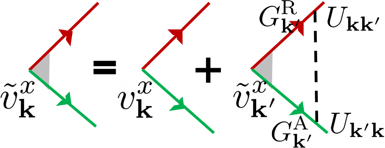
For pseudospin-1 fermions, the ladder diagram correction to velocity should be considered. The diagram describes the iterative equation for the corrected velocity v ~ k ′ x subscript superscript ~ 𝑣 𝑥 superscript k ′ \tilde{v}^{x}_{\textbf{k}^{\prime}}
Figure 7: The diagram for the vertex correction to the velocity, The arrow lines are for Green’s functions. The dashed lines are for disorder scattering ( U ) 𝑈 (U)
v ~ 𝐤 i = v 𝐤 i + ∑ 𝐤 ′ G 𝐤 ′ R G 𝐤 ′ A ⟨ U 𝐤 , 𝐤 ′ U 𝐤 ′ , 𝐤 ⟩ i m p v ~ 𝐤 ′ i , superscript subscript ~ 𝑣 𝐤 𝑖 superscript subscript 𝑣 𝐤 𝑖 subscript superscript 𝐤 ′ superscript subscript 𝐺 superscript 𝐤 ′ R superscript subscript 𝐺 superscript 𝐤 ′ A subscript delimited-⟨⟩ subscript 𝑈 𝐤 superscript 𝐤 ′
subscript 𝑈 superscript 𝐤 ′ 𝐤
𝑖 𝑚 𝑝 superscript subscript ~ 𝑣 superscript 𝐤 ′ 𝑖 \tilde{v}_{\mathbf{k}}^{i}=v_{\mathbf{k}}^{i}+\sum_{\mathbf{k}^{\prime}}G_{\mathbf{k}^{\prime}}^{\mathrm{R}}G_{\mathbf{k}^{\prime}}^{\mathrm{A}}\left\langle U_{\mathbf{k},\mathbf{k}^{\prime}}U_{\mathbf{k}^{\prime},\mathbf{k}}\right\rangle_{imp}\tilde{v}_{\mathbf{k}^{\prime}}^{i}, (44)
where i = x / y 𝑖 𝑥 𝑦 i=x/y η v subscript 𝜂 𝑣 \eta_{v}
v ~ 𝐤 i = η v v 𝐤 i , superscript subscript ~ 𝑣 𝐤 𝑖 subscript 𝜂 𝑣 superscript subscript 𝑣 𝐤 𝑖 \tilde{v}_{\mathbf{k}}^{i}=\eta_{v}v_{\mathbf{k}}^{i}, (45)
where the bare velocity v 𝐤 x = v F cos ϕ superscript subscript 𝑣 𝐤 𝑥 subscript 𝑣 𝐹 italic-ϕ v_{\mathbf{k}}^{x}=v_{F}\cos\phi v 𝐤 y = v F sin ϕ superscript subscript 𝑣 𝐤 𝑦 subscript 𝑣 𝐹 italic-ϕ v_{\mathbf{k}}^{y}=v_{F}\sin\phi
v ~ k x = v 𝐤 x + ∫ 0 ∞ k ′ d k ′ 2 π G 𝐤 ′ R G 𝐤 ′ A ∫ 0 2 π d ϕ ′ 2 π η v v F cos ϕ ′ ⟨ U 𝐤 , 𝐤 ′ U 𝐤 ′ , 𝐤 ⟩ i m p , subscript superscript ~ 𝑣 𝑥 k superscript subscript 𝑣 𝐤 𝑥 superscript subscript 0 superscript 𝑘 ′ 𝑑 superscript 𝑘 ′ 2 𝜋 superscript subscript 𝐺 superscript 𝐤 ′ R superscript subscript 𝐺 superscript 𝐤 ′ A superscript subscript 0 2 𝜋 𝑑 superscript italic-ϕ ′ 2 𝜋 subscript 𝜂 𝑣 subscript 𝑣 𝐹 superscript italic-ϕ ′ subscript delimited-⟨⟩ subscript 𝑈 𝐤 superscript 𝐤 ′
subscript 𝑈 superscript 𝐤 ′ 𝐤
𝑖 𝑚 𝑝 \tilde{v}^{x}_{\textbf{k}}=v_{\mathbf{k}}^{x}+\int_{0}^{\infty}\frac{k^{\prime}dk^{\prime}}{2\pi}G_{\mathbf{k}^{\prime}}^{\mathrm{R}}G_{\mathbf{k}^{\prime}}^{\mathrm{A}}\int_{0}^{2\pi}\frac{d\phi^{\prime}}{2\pi}\eta_{v}v_{F}\cos\phi^{\prime}\left\langle U_{\mathbf{k},\mathbf{k}^{\prime}}U_{\mathbf{k}^{\prime},\mathbf{k}}\right\rangle_{imp}, (46)
I = ∫ 0 ∞ k ′ d k ′ 2 π G 𝐤 ′ R G 𝐤 ′ A = N F ∫ − ∞ ∞ 𝑑 ϵ 𝐤 1 ( ω − ϵ k + i ℏ 2 τ ) 1 ( ω − ϵ k − i ℏ 2 τ ) , 𝐼 superscript subscript 0 superscript 𝑘 ′ 𝑑 superscript 𝑘 ′ 2 𝜋 superscript subscript 𝐺 superscript 𝐤 ′ R superscript subscript 𝐺 superscript 𝐤 ′ A subscript 𝑁 𝐹 superscript subscript differential-d subscript italic-ϵ 𝐤 1 𝜔 subscript italic-ϵ k 𝑖 Planck-constant-over-2-pi 2 𝜏 1 𝜔 subscript italic-ϵ k 𝑖 Planck-constant-over-2-pi 2 𝜏 I=\int_{0}^{\infty}\frac{k^{\prime}dk^{\prime}}{2\pi}G_{\mathbf{k}^{\prime}}^{\mathrm{R}}G_{\mathbf{k}^{\prime}}^{\mathrm{A}}\\
=N_{F}\int_{-\infty}^{\infty}d\epsilon_{\mathbf{{k}}}\frac{1}{(\omega-\epsilon_{\textbf{k}}+i\frac{\hbar}{2\tau})}\frac{1}{(\omega-\epsilon_{\textbf{k}}-i\frac{\hbar}{2\tau})},\\
(47)
poles are given by
ϵ 𝐤 = ( ω − ϵ k − i ℏ 2 τ ) , ( ω − ϵ k + i ℏ 2 τ ) subscript italic-ϵ 𝐤 𝜔 subscript italic-ϵ k 𝑖 Planck-constant-over-2-pi 2 𝜏 𝜔 subscript italic-ϵ k 𝑖 Planck-constant-over-2-pi 2 𝜏
\displaystyle\epsilon_{\mathbf{{k}}}=\left(\omega-\epsilon_{\textbf{k}}-i\frac{\hbar}{2\tau}\right),\ \left(\omega-\epsilon_{\textbf{k}}+i\frac{\hbar}{2\tau}\right) (48)
above integral is solved by closing the contour in the upper half of the complex plane and using the residue theorem
The residue at ( ω + i ℏ 2 τ ) 𝜔 𝑖 Planck-constant-over-2-pi 2 𝜏 (\omega+i\frac{\hbar}{2\tau}) τ i ℏ 𝜏 𝑖 Planck-constant-over-2-pi \frac{\tau}{i\hbar}
I = 2 π i × N F τ i ℏ = 2 π N F τ ℏ . 𝐼 2 𝜋 𝑖 subscript 𝑁 𝐹 𝜏 𝑖 Planck-constant-over-2-pi 2 𝜋 subscript 𝑁 𝐹 𝜏 Planck-constant-over-2-pi \displaystyle I=2\pi i\times\frac{N_{F}\tau}{i\hbar}=\frac{2\pi N_{F}\tau}{\hbar}. (49)
Substituting the above results in Eq. 46
v ~ k x = v 𝐤 i + 2 π N F τ ℏ η v v F ∫ 0 2 π d ϕ ′ 2 π cos ϕ ′ ⟨ U 𝐤 , 𝐤 ′ U 𝐤 ′ , 𝐤 ⟩ i m p , subscript superscript ~ 𝑣 𝑥 k superscript subscript 𝑣 𝐤 𝑖 2 𝜋 subscript 𝑁 𝐹 𝜏 Planck-constant-over-2-pi subscript 𝜂 𝑣 subscript 𝑣 𝐹 superscript subscript 0 2 𝜋 𝑑 superscript italic-ϕ ′ 2 𝜋 superscript italic-ϕ ′ subscript delimited-⟨⟩ subscript 𝑈 𝐤 superscript 𝐤 ′
subscript 𝑈 superscript 𝐤 ′ 𝐤
𝑖 𝑚 𝑝 \tilde{v}^{x}_{\textbf{k}}=v_{\mathbf{k}}^{i}+\frac{2\pi N_{F}\tau}{\hbar}\eta_{v}v_{F}\int_{0}^{2\pi}\frac{d\phi^{\prime}}{2\pi}\cos\phi^{\prime}\left\langle U_{\mathbf{k},\mathbf{k}^{\prime}}U_{\mathbf{k}^{\prime},\mathbf{k}}\right\rangle_{imp}, (50)
where we have
∫ 0 2 π d ϕ ′ 2 π cos ϕ ′ ⟨ U 𝐤 , 𝐤 ′ U 𝐤 ′ , 𝐤 ⟩ i m p = superscript subscript 0 2 𝜋 𝑑 superscript italic-ϕ ′ 2 𝜋 superscript italic-ϕ ′ subscript delimited-⟨⟩ subscript 𝑈 𝐤 superscript 𝐤 ′
subscript 𝑈 superscript 𝐤 ′ 𝐤
𝑖 𝑚 𝑝 absent \displaystyle\int_{0}^{2\pi}\frac{d\phi^{\prime}}{2\pi}\cos\phi^{\prime}\left\langle U_{\mathbf{k},\mathbf{k}^{\prime}}U_{\mathbf{k}^{\prime},\mathbf{k}}\right\rangle_{imp}=
∫ 0 2 π d ϕ ′ 2 π cos ϕ ′ [ ⟨ U 𝐤 , 𝐤 ′ U 𝐤 ′ , 𝐤 ⟩ e + ⟨ U 𝐤 , 𝐤 ′ U 𝐤 ′ , 𝐤 ⟩ x + ⟨ U 𝐤 , 𝐤 ′ U 𝐤 ′ , 𝐤 ⟩ y + ⟨ U 𝐤 , 𝐤 ′ U 𝐤 ′ , 𝐤 ⟩ z ] superscript subscript 0 2 𝜋 𝑑 superscript italic-ϕ ′ 2 𝜋 superscript italic-ϕ ′ delimited-[] subscript delimited-⟨⟩ subscript 𝑈 𝐤 superscript 𝐤 ′
subscript 𝑈 superscript 𝐤 ′ 𝐤
𝑒 subscript delimited-⟨⟩ subscript 𝑈 𝐤 superscript 𝐤 ′
subscript 𝑈 superscript 𝐤 ′ 𝐤
𝑥 subscript delimited-⟨⟩ subscript 𝑈 𝐤 superscript 𝐤 ′
subscript 𝑈 superscript 𝐤 ′ 𝐤
𝑦 subscript delimited-⟨⟩ subscript 𝑈 𝐤 superscript 𝐤 ′
subscript 𝑈 superscript 𝐤 ′ 𝐤
𝑧 \displaystyle\int_{0}^{2\pi}\frac{d\phi^{\prime}}{2\pi}\cos\phi^{\prime}\left[\left\langle U_{\mathbf{k},\mathbf{k}^{\prime}}U_{\mathbf{k}^{\prime},\mathbf{k}}\right\rangle_{e}+\left\langle U_{\mathbf{k},\mathbf{k}^{\prime}}U_{\mathbf{k}^{\prime},\mathbf{k}}\right\rangle_{x}+\left\langle U_{\mathbf{k},\mathbf{k}^{\prime}}U_{\mathbf{k}^{\prime},\mathbf{k}}\right\rangle_{y}+\left\langle U_{\mathbf{k},\mathbf{k}^{\prime}}U_{\mathbf{k}^{\prime},\mathbf{k}}\right\rangle_{z}\right] (51)
∫ 0 2 π d ϕ ′ 2 π cos ϕ ′ ⟨ U 𝐤 , 𝐤 ′ U 𝐤 ′ , 𝐤 ⟩ e = superscript subscript 0 2 𝜋 𝑑 superscript italic-ϕ ′ 2 𝜋 superscript italic-ϕ ′ subscript delimited-⟨⟩ subscript 𝑈 𝐤 superscript 𝐤 ′
subscript 𝑈 superscript 𝐤 ′ 𝐤
𝑒 absent \displaystyle\int_{0}^{2\pi}\frac{d\phi^{\prime}}{2\pi}\cos\phi^{\prime}\left\langle U_{\mathbf{k},\mathbf{k}^{\prime}}U_{\mathbf{k}^{\prime},\mathbf{k}}\right\rangle_{e}=
n 0 u 0 2 2 ∫ 0 2 π d ϕ ′ 2 π cos ϕ ′ [ ( a 4 + b 4 + 1 ) 2 + cos ( ϕ − ϕ ′ ) + a 2 b 2 cos 2 ( ϕ − ϕ ′ ) ] = subscript 𝑛 0 superscript subscript 𝑢 0 2 2 superscript subscript 0 2 𝜋 𝑑 superscript italic-ϕ ′ 2 𝜋 superscript italic-ϕ ′ delimited-[] superscript 𝑎 4 superscript 𝑏 4 1 2 italic-ϕ superscript italic-ϕ ′ superscript 𝑎 2 superscript 𝑏 2 2 italic-ϕ superscript italic-ϕ ′ absent \displaystyle\frac{n_{0}u_{0}^{2}}{2}\int_{0}^{2\pi}\frac{d\phi^{\prime}}{2\pi}\cos\phi^{\prime}\left[\frac{(a^{4}+b^{4}+1)}{2}+\cos(\phi-\phi^{\prime})+a^{2}b^{2}\cos 2(\phi-\phi^{\prime})\right]=
n 0 u 0 2 2 ∫ 0 2 π d ϕ ′ 2 π cos ϕ ′ cos ( ϕ − ϕ ′ ) = n 0 u 0 2 4 cos ϕ subscript 𝑛 0 superscript subscript 𝑢 0 2 2 superscript subscript 0 2 𝜋 𝑑 superscript italic-ϕ ′ 2 𝜋 superscript italic-ϕ ′ italic-ϕ superscript italic-ϕ ′ subscript 𝑛 0 superscript subscript 𝑢 0 2 4 italic-ϕ \displaystyle\frac{n_{0}u_{0}^{2}}{2}\int_{0}^{2\pi}\frac{d\phi^{\prime}}{2\pi}\cos\phi^{\prime}\cos(\phi-\phi^{\prime})=\frac{n_{0}u_{0}^{2}}{4}\cos\phi (52)
∫ 0 2 π d ϕ ′ 2 π cos ϕ ′ ⟨ U 𝐤 , 𝐤 ′ U 𝐤 ′ , 𝐤 ⟩ x = superscript subscript 0 2 𝜋 𝑑 superscript italic-ϕ ′ 2 𝜋 superscript italic-ϕ ′ subscript delimited-⟨⟩ subscript 𝑈 𝐤 superscript 𝐤 ′
subscript 𝑈 superscript 𝐤 ′ 𝐤
𝑥 absent \displaystyle\int_{0}^{2\pi}\frac{d\phi^{\prime}}{2\pi}\cos\phi^{\prime}\left\langle U_{\mathbf{k},\mathbf{k}^{\prime}}U_{\mathbf{k}^{\prime},\mathbf{k}}\right\rangle_{x}=
n m u x 2 2 ∫ 0 2 π d ϕ ′ 2 π cos ϕ ′ [ 1 + cos ( ϕ + ϕ ′ ) + a b ( 2 cos ( ϕ − ϕ ′ ) + cos 2 ϕ + cos 2 ϕ ′ ) ] subscript 𝑛 𝑚 subscript superscript 𝑢 2 𝑥 2 superscript subscript 0 2 𝜋 𝑑 superscript italic-ϕ ′ 2 𝜋 superscript italic-ϕ ′ delimited-[] 1 italic-ϕ superscript italic-ϕ ′ 𝑎 𝑏 2 italic-ϕ superscript italic-ϕ ′ 2 italic-ϕ 2 superscript italic-ϕ ′ \displaystyle\frac{n_{m}u^{2}_{x}}{2}\int_{0}^{2\pi}\frac{d\phi^{\prime}}{2\pi}\cos\phi^{\prime}\left[1+\cos(\phi+\phi^{\prime})+ab(2\cos(\phi-\phi^{\prime})+\cos 2\phi+\cos 2\phi^{\prime})\right] (53)
= n m u x 2 4 ( 1 + 2 a b ) cos ϕ absent subscript 𝑛 𝑚 subscript superscript 𝑢 2 𝑥 4 1 2 𝑎 𝑏 italic-ϕ =\frac{n_{m}u^{2}_{x}}{4}(1+2ab)\cos\phi (54)
∫ 0 2 π d ϕ ′ 2 π cos ϕ ′ ⟨ U 𝐤 , 𝐤 ′ U 𝐤 ′ , 𝐤 ⟩ y = superscript subscript 0 2 𝜋 𝑑 superscript italic-ϕ ′ 2 𝜋 superscript italic-ϕ ′ subscript delimited-⟨⟩ subscript 𝑈 𝐤 superscript 𝐤 ′
subscript 𝑈 superscript 𝐤 ′ 𝐤
𝑦 absent \displaystyle\int_{0}^{2\pi}\frac{d\phi^{\prime}}{2\pi}\cos\phi^{\prime}\left\langle U_{\mathbf{k},\mathbf{k}^{\prime}}U_{\mathbf{k}^{\prime},\mathbf{k}}\right\rangle_{y}=
n m u y 2 2 ∫ 0 2 π d ϕ ′ 2 π cos ϕ ′ [ 1 − cos ( ϕ + ϕ ′ ) + a b ( 2 cos ( ϕ − ϕ ′ ) − cos 2 ϕ − cos 2 ϕ ′ ) ] subscript 𝑛 𝑚 subscript superscript 𝑢 2 𝑦 2 superscript subscript 0 2 𝜋 𝑑 superscript italic-ϕ ′ 2 𝜋 superscript italic-ϕ ′ delimited-[] 1 italic-ϕ superscript italic-ϕ ′ 𝑎 𝑏 2 italic-ϕ superscript italic-ϕ ′ 2 italic-ϕ 2 superscript italic-ϕ ′ \displaystyle\frac{n_{m}u^{2}_{y}}{2}\int_{0}^{2\pi}\frac{d\phi^{\prime}}{2\pi}\cos\phi^{\prime}\left[1-\cos(\phi+\phi^{\prime})+ab(2\cos(\phi-\phi^{\prime})-\cos 2\phi-\cos 2\phi^{\prime})\right] (55)
= − n m u y 2 4 ( 1 − 2 a b ) cos ϕ absent subscript 𝑛 𝑚 subscript superscript 𝑢 2 𝑦 4 1 2 𝑎 𝑏 italic-ϕ =-\frac{n_{m}u^{2}_{y}}{4}(1-2ab)\cos\phi (56)
∫ 0 2 π d ϕ ′ 2 π cos ϕ ′ ⟨ U 𝐤 , 𝐤 ′ U 𝐤 ′ , 𝐤 ⟩ z = 0 , superscript subscript 0 2 𝜋 𝑑 superscript italic-ϕ ′ 2 𝜋 superscript italic-ϕ ′ subscript delimited-⟨⟩ subscript 𝑈 𝐤 superscript 𝐤 ′
subscript 𝑈 superscript 𝐤 ′ 𝐤
𝑧 0 \int_{0}^{2\pi}\frac{d\phi^{\prime}}{2\pi}\cos\phi^{\prime}\left\langle U_{\mathbf{k},\mathbf{k}^{\prime}}U_{\mathbf{k}^{\prime},\mathbf{k}}\right\rangle_{z}=0, (57)
now Eq. 50
η v = 1 + 2 π N F τ ℏ η v [ n 0 u 0 2 4 + n m u x 2 4 ( 1 + 2 a b ) − n m u y 2 4 ( 1 − 2 a b ) ] subscript 𝜂 𝑣 1 2 𝜋 subscript 𝑁 𝐹 𝜏 Planck-constant-over-2-pi subscript 𝜂 𝑣 delimited-[] subscript 𝑛 0 superscript subscript 𝑢 0 2 4 subscript 𝑛 𝑚 subscript superscript 𝑢 2 𝑥 4 1 2 𝑎 𝑏 subscript 𝑛 𝑚 subscript superscript 𝑢 2 𝑦 4 1 2 𝑎 𝑏 \eta_{v}=1+\frac{2\pi N_{F}\tau}{\hbar}\eta_{v}\left[\frac{n_{0}u_{0}^{2}}{4}+\frac{n_{m}u^{2}_{x}}{4}(1+2ab)\ -\frac{n_{m}u^{2}_{y}}{4}(1-2ab)\right] (58)
where we have,
n 0 u 0 2 4 = ℏ 2 π N F τ e ( a 4 + b 4 + 1 ) , subscript 𝑛 0 superscript subscript 𝑢 0 2 4 Planck-constant-over-2-pi 2 𝜋 subscript 𝑁 𝐹 subscript 𝜏 𝑒 superscript 𝑎 4 superscript 𝑏 4 1 \displaystyle\frac{n_{0}u_{0}^{2}}{4}=\frac{\hbar}{2\pi N_{F}\tau_{e}(a^{4}+b^{4}+1)},
n m u x 2 4 = ℏ 4 π N F τ m , x ( 1 + a b cos 2 ϕ ) , subscript 𝑛 𝑚 subscript superscript 𝑢 2 𝑥 4 Planck-constant-over-2-pi 4 𝜋 subscript 𝑁 𝐹 subscript 𝜏 𝑚 𝑥
1 𝑎 𝑏 2 italic-ϕ \displaystyle\frac{n_{m}u^{2}_{x}}{4}=\frac{\hbar}{4\pi N_{F}\tau_{m,x}(1+ab\cos 2\phi)},
n m u y 2 4 = ℏ 4 π N F τ m , y ( 1 − a b cos 2 ϕ ) . subscript 𝑛 𝑚 subscript superscript 𝑢 2 𝑦 4 Planck-constant-over-2-pi 4 𝜋 subscript 𝑁 𝐹 subscript 𝜏 𝑚 𝑦
1 𝑎 𝑏 2 italic-ϕ \displaystyle\frac{n_{m}u^{2}_{y}}{4}=\frac{\hbar}{4\pi N_{F}\tau_{m,y}(1-ab\cos 2\phi)}. (59)
Using the above relations, we get,
η v = 1 + η v [ τ τ e ( a 4 + b 4 + 1 ) + τ ( 1 + 2 a b ) 2 τ m , x ( 1 + a b cos 2 ϕ ) − τ ( 1 − 2 a b ) 2 τ m , y ( 1 − a b cos 2 ϕ ) ] , subscript 𝜂 𝑣 1 subscript 𝜂 𝑣 delimited-[] 𝜏 subscript 𝜏 𝑒 superscript 𝑎 4 superscript 𝑏 4 1 𝜏 1 2 𝑎 𝑏 2 subscript 𝜏 𝑚 𝑥
1 𝑎 𝑏 2 italic-ϕ 𝜏 1 2 𝑎 𝑏 2 subscript 𝜏 𝑚 𝑦
1 𝑎 𝑏 2 italic-ϕ \eta_{v}=1+\eta_{v}\left[\frac{\tau}{\tau_{e}(a^{4}+b^{4}+1)}+\frac{\tau(1+2ab)}{2\tau_{m,x}(1+ab\cos 2\phi)}-\frac{\tau(1-2ab)}{2\tau_{m,y}(1-ab\cos 2\phi)}\right], (60)
finally, the vertex correction factor is given by,
η v = 1 1 − [ τ τ e ( a 4 + b 4 + 1 ) + τ ( 1 + 2 a b ) 2 τ m , x ( 1 + a b cos 2 ϕ ) − τ ( 1 − 2 a b ) 2 τ m , y ( 1 − a b cos 2 ϕ ) ] . subscript 𝜂 𝑣 1 1 delimited-[] 𝜏 subscript 𝜏 𝑒 superscript 𝑎 4 superscript 𝑏 4 1 𝜏 1 2 𝑎 𝑏 2 subscript 𝜏 𝑚 𝑥
1 𝑎 𝑏 2 italic-ϕ 𝜏 1 2 𝑎 𝑏 2 subscript 𝜏 𝑚 𝑦
1 𝑎 𝑏 2 italic-ϕ \eta_{v}=\frac{1}{1-\left[\frac{\tau}{\tau_{e}(a^{4}+b^{4}+1)}+\frac{\tau(1+2ab)}{2\tau_{m,x}(1+ab\cos 2\phi)}-\frac{\tau(1-2ab)}{2\tau_{m,y}(1-ab\cos 2\phi)}\right]}. (61)
If we assume in-plane isotropy u x = u y subscript 𝑢 𝑥 subscript 𝑢 𝑦 u_{x}=u_{y}
η v = 1 + 2 π N F τ ℏ η v [ n 0 u 0 2 4 + n m u x 2 ( a b ) ] subscript 𝜂 𝑣 1 2 𝜋 subscript 𝑁 𝐹 𝜏 Planck-constant-over-2-pi subscript 𝜂 𝑣 delimited-[] subscript 𝑛 0 superscript subscript 𝑢 0 2 4 subscript 𝑛 𝑚 subscript superscript 𝑢 2 𝑥 𝑎 𝑏 \displaystyle\eta_{v}=1+\frac{2\pi N_{F}\tau}{\hbar}\eta_{v}\left[\frac{n_{0}u_{0}^{2}}{4}+n_{m}u^{2}_{x}(ab)\right]
η v = 1 + η v [ τ τ e ( a 4 + b 4 + 1 ) + ( 2 a b ) τ τ m , x ] subscript 𝜂 𝑣 1 subscript 𝜂 𝑣 delimited-[] 𝜏 subscript 𝜏 𝑒 superscript 𝑎 4 superscript 𝑏 4 1 2 𝑎 𝑏 𝜏 subscript 𝜏 𝑚 𝑥
\displaystyle\eta_{v}=1+\eta_{v}\left[\frac{\tau}{\tau_{e}(a^{4}+b^{4}+1)}+(2ab)\frac{\tau}{\tau_{m,x}}\right]
η v = 1 1 − [ τ τ e ( a 4 + b 4 + 1 ) + ( 2 a b ) τ τ m , x ] . subscript 𝜂 𝑣 1 1 delimited-[] 𝜏 subscript 𝜏 𝑒 superscript 𝑎 4 superscript 𝑏 4 1 2 𝑎 𝑏 𝜏 subscript 𝜏 𝑚 𝑥
\displaystyle\eta_{v}=\frac{1}{1-\left[\frac{\tau}{\tau_{e}(a^{4}+b^{4}+1)}+(2ab)\frac{\tau}{\tau_{m,x}}\right]}. (62)
V Bare and dressed Hikami boxes
The quantum interference correction to conductivity is obtained by the calculation of bare Hiakmi box and two dressed Hikami boxes.
V.1 Bare Hikami box
The bare Hikami box at zero temperature is calculated as
σ 0 F = e 2 ℏ 2 π ∑ q Γ ( q ) ∑ k v ~ k x v ~ q-k x G 𝐤 R G 𝐤 A G 𝐪 − 𝐤 R G 𝐪 − 𝐤 A , superscript subscript 𝜎 0 𝐹 superscript 𝑒 2 Planck-constant-over-2-pi 2 𝜋 subscript q Γ q subscript k superscript subscript ~ 𝑣 k 𝑥 subscript superscript ~ 𝑣 𝑥 q-k superscript subscript 𝐺 𝐤 R superscript subscript 𝐺 𝐤 A superscript subscript 𝐺 𝐪 𝐤 R superscript subscript 𝐺 𝐪 𝐤 A \sigma_{0}^{F}=\frac{e^{2}\hbar}{2\pi}\sum_{\textbf{q}}\Gamma(\textbf{q})\sum_{\textbf{k}}\tilde{v}_{\textbf{k}}^{x}\tilde{v}^{x}_{\textbf{q-k}}G_{\mathbf{k}}^{\mathrm{R}}G_{\mathbf{k}}^{\mathrm{A}}G_{\mathbf{q-k}}^{\mathrm{R}}G_{\mathbf{q-k}}^{\mathrm{A}}, (63)
Figure 8: The diagrams for the quantum interference
correction to conductivity of pseudospin-1 fermions. The arrowed
solid and dashed lines represent the Green’s functions and
impurity scattering, respectively. (a) The bare and
(b) two dressed Hikami boxes give the quantum conductivity
correction from the maximally crossed diagrams.
retarded and advanced Green’s function is given by
G 𝐤 R / A ( ω ) = 1 ω − ϵ k ± i ℏ 2 τ , G 𝐪 − 𝐤 R / A ( ω ) = 1 ω − ϵ 𝐪 − 𝐤 ± i ℏ 2 τ formulae-sequence subscript superscript 𝐺 𝑅 𝐴 𝐤 𝜔 1 plus-or-minus 𝜔 subscript italic-ϵ k 𝑖 Planck-constant-over-2-pi 2 𝜏 subscript superscript 𝐺 𝑅 𝐴 𝐪 𝐤 𝜔 1 plus-or-minus 𝜔 subscript italic-ϵ 𝐪 𝐤 𝑖 Planck-constant-over-2-pi 2 𝜏 \displaystyle G^{R/A}_{\mathbf{k}}(\omega)=\frac{1}{\omega-\epsilon_{\textbf{k}}\pm i\frac{\hbar}{2\tau}},\ G^{R/A}_{\mathbf{q-k}}(\omega)=\frac{1}{\omega-\epsilon_{\mathbf{q-k}}\pm i\frac{\hbar}{2\tau}} (64)
In the small 𝐪 𝐪 \mathbf{q}
ϵ 𝐪 − 𝐤 ≈ ϵ k − ℏ 𝐯 𝐅 . 𝐪 , formulae-sequence subscript italic-ϵ 𝐪 𝐤 subscript italic-ϵ k Planck-constant-over-2-pi subscript 𝐯 𝐅 𝐪 \epsilon_{\mathbf{q-k}}\approx\epsilon_{\textbf{k}}-\hbar\mathbf{v_{F}.q}, (65)
Γ ( q ) Γ q \Gamma(\textbf{q}) 𝐪 𝐪 \mathbf{q} 𝐪 𝐪 \mathbf{q} 𝐤 𝐤 \mathbf{k} 𝐪 = 0 𝐪 0 \mathbf{q}=0
σ 0 F = e 2 ℏ η v 2 v F 2 2 π ∑ q Γ ( q ) ∑ k cos ϕ cos ( ϕ − θ ) G 𝐤 R G 𝐤 A G 𝐪 − 𝐤 R G 𝐪 − 𝐤 A superscript subscript 𝜎 0 𝐹 superscript 𝑒 2 Planck-constant-over-2-pi subscript superscript 𝜂 2 𝑣 subscript superscript 𝑣 2 𝐹 2 𝜋 subscript q Γ q subscript k italic-ϕ italic-ϕ 𝜃 superscript subscript 𝐺 𝐤 R superscript subscript 𝐺 𝐤 A superscript subscript 𝐺 𝐪 𝐤 R superscript subscript 𝐺 𝐪 𝐤 A \displaystyle\sigma_{0}^{F}=\frac{e^{2}\hbar\eta^{2}_{v}v^{2}_{F}}{2\pi}\sum_{\textbf{q}}\Gamma(\textbf{q})\sum_{\textbf{k}}\cos\phi\cos(\phi-\theta)G_{\mathbf{k}}^{\mathrm{R}}G_{\mathbf{k}}^{\mathrm{A}}G_{\mathbf{q-k}}^{\mathrm{R}}G_{\mathbf{q-k}}^{\mathrm{A}} (66)
= e 2 ℏ η v 2 v F 2 2 π ∫ 0 ∞ k d k 2 π G 𝐤 R G 𝐤 A G 𝐪 − 𝐤 R G 𝐪 − 𝐤 A ∫ 0 2 π d ϕ 2 π cos ϕ cos ( ϕ − θ ) . absent superscript 𝑒 2 Planck-constant-over-2-pi subscript superscript 𝜂 2 𝑣 subscript superscript 𝑣 2 𝐹 2 𝜋 superscript subscript 0 𝑘 𝑑 𝑘 2 𝜋 superscript subscript 𝐺 𝐤 R superscript subscript 𝐺 𝐤 A superscript subscript 𝐺 𝐪 𝐤 R superscript subscript 𝐺 𝐪 𝐤 A superscript subscript 0 2 𝜋 𝑑 italic-ϕ 2 𝜋 italic-ϕ italic-ϕ 𝜃 \displaystyle=\frac{e^{2}\hbar\eta^{2}_{v}v^{2}_{F}}{2\pi}\int_{0}^{\infty}\frac{kdk}{2\pi}G_{\mathbf{k}}^{\mathrm{R}}G_{\mathbf{k}}^{\mathrm{A}}G_{\mathbf{q-k}}^{\mathrm{R}}G_{\mathbf{q-k}}^{\mathrm{A}}\int_{0}^{2\pi}\frac{d\phi}{2\pi}\cos\phi\cos(\phi-\theta). (67)
Let’s assume that
I = ∫ 0 ∞ k d k 2 π G 𝐤 R G 𝐤 A G 𝐪 − 𝐤 R G 𝐪 − 𝐤 A , 𝐼 superscript subscript 0 𝑘 𝑑 𝑘 2 𝜋 superscript subscript 𝐺 𝐤 R superscript subscript 𝐺 𝐤 A superscript subscript 𝐺 𝐪 𝐤 R superscript subscript 𝐺 𝐪 𝐤 A \displaystyle I=\int_{0}^{\infty}\frac{kdk}{2\pi}G_{\mathbf{k}}^{\mathrm{R}}G_{\mathbf{k}}^{\mathrm{A}}G_{\mathbf{q-k}}^{\mathrm{R}}G_{\mathbf{q-k}}^{\mathrm{A}}, (68)
= N F ∫ − ∞ ∞ 𝑑 ϵ 𝐤 G 𝐤 R G 𝐤 A G 𝐪 − 𝐤 R G 𝐪 − 𝐤 A absent subscript 𝑁 𝐹 superscript subscript differential-d subscript italic-ϵ 𝐤 superscript subscript 𝐺 𝐤 R superscript subscript 𝐺 𝐤 A superscript subscript 𝐺 𝐪 𝐤 R superscript subscript 𝐺 𝐪 𝐤 A \displaystyle=N_{F}\int_{-\infty}^{\infty}d\epsilon_{\mathbf{k}}G_{\mathbf{k}}^{\mathrm{R}}G_{\mathbf{k}}^{\mathrm{A}}G_{\mathbf{q-k}}^{\mathrm{R}}G_{\mathbf{q-k}}^{\mathrm{A}} (69)
= N F ∫ − ∞ ∞ 𝑑 ϵ 𝐤 1 ( ω − ϵ 𝐤 + i ℏ 2 τ ) 1 ( ω − ϵ 𝐤 − i ℏ 2 τ ) 1 ( ω − ϵ 𝐤 + ℏ 𝐯 𝐅 . 𝐪 + i ℏ 2 τ ) 1 ( ω − ϵ 𝐤 + ℏ 𝐯 𝐅 . 𝐪 − i ℏ 2 τ ) absent subscript 𝑁 𝐹 superscript subscript differential-d subscript italic-ϵ 𝐤 1 𝜔 subscript italic-ϵ 𝐤 𝑖 Planck-constant-over-2-pi 2 𝜏 1 𝜔 subscript italic-ϵ 𝐤 𝑖 Planck-constant-over-2-pi 2 𝜏 1 formulae-sequence 𝜔 subscript italic-ϵ 𝐤 Planck-constant-over-2-pi subscript 𝐯 𝐅 𝐪 𝑖 Planck-constant-over-2-pi 2 𝜏 1 formulae-sequence 𝜔 subscript italic-ϵ 𝐤 Planck-constant-over-2-pi subscript 𝐯 𝐅 𝐪 𝑖 Planck-constant-over-2-pi 2 𝜏 \displaystyle=N_{F}\int_{-\infty}^{\infty}d\epsilon_{\mathbf{k}}\frac{1}{(\omega-\epsilon_{\mathbf{k}}+\frac{i\hbar}{2\tau})}\frac{1}{(\omega-\epsilon_{\mathbf{k}}-\frac{i\hbar}{2\tau})}\frac{1}{(\omega-\epsilon_{\mathbf{k}}+\hbar\mathbf{v_{F}.q}+\frac{i\hbar}{2\tau})}\frac{1}{(\omega-\epsilon_{\mathbf{k}}+\hbar\mathbf{v_{F}.q}-\frac{i\hbar}{2\tau})} (70)
using the technique of contour integration, poles are
ϵ 𝐤 = ω + i ℏ 2 τ ; ω − i ℏ 2 τ ; ω + ℏ 𝐯 𝐅 ⋅ 𝐪 + i ℏ 2 τ ; ω + ℏ 𝐯 𝐅 ⋅ 𝐪 − i ℏ 2 τ subscript italic-ϵ 𝐤 𝜔 𝑖 Planck-constant-over-2-pi 2 𝜏 𝜔 𝑖 Planck-constant-over-2-pi 2 𝜏 𝜔 ⋅ Planck-constant-over-2-pi subscript 𝐯 𝐅 𝐪 𝑖 Planck-constant-over-2-pi 2 𝜏 𝜔 ⋅ Planck-constant-over-2-pi subscript 𝐯 𝐅 𝐪 𝑖 Planck-constant-over-2-pi 2 𝜏
\displaystyle\epsilon_{\mathbf{k}}=\omega+\frac{i\hbar}{2\tau};\ \omega-\frac{i\hbar}{2\tau};\ \omega+\hbar\mathbf{v_{F}\cdot q}+\frac{i\hbar}{2\tau};\ \omega+\hbar\mathbf{v_{F}\cdot q}-\frac{i\hbar}{2\tau} (71)
contour is closed in the upper half of the complex plane, and the sum of residues is given by,
•
residue at ϵ 𝐤 = ω + i ℏ 2 τ subscript italic-ϵ 𝐤 𝜔 𝑖 Planck-constant-over-2-pi 2 𝜏 \epsilon_{\mathbf{k}}=\omega+\frac{i\hbar}{2\tau}
1 i ℏ τ ( − ℏ 𝐯 𝐅 . 𝐪 ) ( i ℏ τ − ℏ 𝐯 𝐅 ⋅ 𝐪 ) \frac{1}{\frac{i\hbar}{\tau}(-\hbar\mathbf{v_{F}.q})(\frac{i\hbar}{\tau}-\hbar\mathbf{v_{F}\cdot q})} (72)
•
residue at ϵ 𝐤 = ω + i ℏ 2 τ + ℏ 𝐯 𝐅 ⋅ 𝐪 subscript italic-ϵ 𝐤 𝜔 𝑖 Planck-constant-over-2-pi 2 𝜏 ⋅ Planck-constant-over-2-pi subscript 𝐯 𝐅 𝐪 \epsilon_{\mathbf{k}}=\omega+\frac{i\hbar}{2\tau}+\hbar\mathbf{v_{F}\cdot q}
1 i ℏ τ ( ℏ 𝐯 𝐅 ⋅ 𝐪 ) ( i ℏ τ + ℏ 𝐯 𝐅 ⋅ 𝐪 ) , 1 𝑖 Planck-constant-over-2-pi 𝜏 ⋅ Planck-constant-over-2-pi subscript 𝐯 𝐅 𝐪 𝑖 Planck-constant-over-2-pi 𝜏 ⋅ Planck-constant-over-2-pi subscript 𝐯 𝐅 𝐪 \frac{1}{\frac{i\hbar}{\tau}(\hbar\mathbf{v_{F}\cdot q})(\frac{i\hbar}{\tau}+\hbar\mathbf{v_{F}\cdot q})}, (73)
the sum of residues is
1 i ℏ τ ( ( ℏ 𝐯 𝐅 ⋅ 𝐪 ) 2 + ℏ 2 τ 2 ) , 1 𝑖 Planck-constant-over-2-pi 𝜏 superscript ⋅ Planck-constant-over-2-pi subscript 𝐯 𝐅 𝐪 2 superscript Planck-constant-over-2-pi 2 superscript 𝜏 2 \frac{1}{\frac{i\hbar}{\tau}((\hbar\mathbf{v_{F}\cdot q})^{2}+\frac{\hbar^{2}}{\tau^{2}})}, (74)
in the limit of 𝐪 → 0 → 𝐪 0 \mathbf{q}\to 0
− 2 τ 3 i ℏ 3 , 2 superscript 𝜏 3 𝑖 superscript Planck-constant-over-2-pi 3 \frac{-2\tau^{3}}{i\hbar^{3}}, (75)
finally, the value of the integral is
I = − 4 π N F τ 3 ℏ 3 . 𝐼 4 𝜋 subscript 𝑁 𝐹 superscript 𝜏 3 superscript Planck-constant-over-2-pi 3 I=\frac{-4\pi N_{F}\tau^{3}}{\hbar^{3}}. (76)
Finally, we obtain:
σ 0 F = − 2 e 2 N F τ 3 η v 2 v F 2 ℏ 2 ∑ q Γ ( q ) ∫ 0 2 π d ϕ 2 π [ cos 2 ϕ cos θ + cos ϕ sin ϕ sin θ ] superscript subscript 𝜎 0 𝐹 2 superscript 𝑒 2 subscript 𝑁 𝐹 superscript 𝜏 3 subscript superscript 𝜂 2 𝑣 subscript superscript 𝑣 2 𝐹 superscript Planck-constant-over-2-pi 2 subscript q Γ q superscript subscript 0 2 𝜋 𝑑 italic-ϕ 2 𝜋 delimited-[] superscript 2 italic-ϕ 𝜃 italic-ϕ italic-ϕ 𝜃 \sigma_{0}^{F}=\frac{-2e^{2}N_{F}\tau^{3}\eta^{2}_{v}v^{2}_{F}}{\hbar^{2}}\sum_{\textbf{q}}\Gamma(\textbf{q})\int_{0}^{2\pi}\frac{d\phi}{2\pi}[\cos^{2}\phi\cos\theta+\cos\phi\sin\phi\sin\theta] (77)
as 𝐪 → 0 → 𝐪 0 \mathbf{q}\to 0 θ → 0 → 𝜃 0 \theta\to 0 → → \to cos θ → 1 → 𝜃 1 \cos\theta\to 1
σ 0 F = − e 2 N F τ 3 η v 2 v F 2 ℏ 2 ∑ q Γ ( q ) superscript subscript 𝜎 0 𝐹 superscript 𝑒 2 subscript 𝑁 𝐹 superscript 𝜏 3 subscript superscript 𝜂 2 𝑣 subscript superscript 𝑣 2 𝐹 superscript Planck-constant-over-2-pi 2 subscript q Γ q \sigma_{0}^{F}=\frac{-e^{2}N_{F}\tau^{3}\eta^{2}_{v}v^{2}_{F}}{\hbar^{2}}\sum_{\textbf{q}}\Gamma(\textbf{q}) (78)
V.2 Two dressed Hikami boxes
Two dressed Hikami boxes denoted as σ R F superscript subscript 𝜎 𝑅 𝐹 \sigma_{R}^{F} σ A F superscript subscript 𝜎 𝐴 𝐹 \sigma_{A}^{F}
σ R F = e 2 ℏ 2 π ∑ q Γ ( q ) ∑ k ∑ k 1 v ~ k x v ~ q − k 1 x G 𝐤 R G 𝐤 𝟏 R G 𝐪 − 𝐤 R G 𝐪 − 𝐤 𝟏 R G 𝐤 A G 𝐪 − 𝐤 𝟏 A ⟨ U 𝐤 1 , k U 𝐪 − 𝐤 𝟏 , 𝐪 − 𝐤 ⟩ i m p , \sigma_{R}^{F}=\frac{e^{2}\hbar}{2\pi}\sum_{\textbf{q}}\Gamma(\textbf{q})\sum_{\textbf{k}}\sum_{\textbf{k}_{1}}\tilde{v}_{\textbf{k}}^{x}\tilde{v}^{x}_{\textbf{q}-\textbf{k}_{1}}G_{\mathbf{k}}^{\mathrm{R}}G_{\mathbf{k_{1}}}^{\mathrm{R}}G_{\mathbf{q-k}}^{\mathrm{R}}G_{\mathbf{q-k_{1}}}^{\mathrm{R}}G_{\mathbf{k}}^{\mathrm{A}}G_{\mathbf{q-k_{1}}}^{\mathrm{A}}\langle U_{\mathbf{k}_{1},\textbf{k}}U_{\mathbf{q-k_{1}},\mathbf{q-k}}\bigl{\rangle}_{imp}, (79)
contribution from small 𝐪 𝐪 \mathbf{q} 𝐤 𝐤 \mathbf{k} q=0
σ R F = e 2 ℏ 2 π ∑ q Γ ( q ) ∑ k v ~ k x G 𝐤 R G 𝐤 A G 𝐪 − 𝐤 R ∑ k 1 v ~ q − k 1 x G 𝐤 𝟏 R G 𝐪 − 𝐤 𝟏 R G 𝐪 − 𝐤 𝟏 A ⟨ U 𝐤 1 , k U 𝐪 − 𝐤 𝟏 , 𝐪 − 𝐤 ⟩ i m p \displaystyle\sigma_{R}^{F}=\frac{e^{2}\hbar}{2\pi}\sum_{\textbf{q}}\Gamma(\textbf{q})\sum_{\textbf{k}}\tilde{v}_{\textbf{k}}^{x}G_{\mathbf{k}}^{\mathrm{R}}G_{\mathbf{k}}^{\mathrm{A}}G_{\mathbf{q-k}}^{\mathrm{R}}\sum_{\textbf{k}_{1}}\tilde{v}^{x}_{\textbf{q}-\textbf{k}_{1}}G_{\mathbf{k_{1}}}^{\mathrm{R}}G_{\mathbf{q-k_{1}}}^{\mathrm{R}}G_{\mathbf{q-k_{1}}}^{\mathrm{A}}\langle U_{\mathbf{k}_{1},\textbf{k}}U_{\mathbf{q-k_{1}},\mathbf{q-k}}\bigl{\rangle}_{imp}
= e 2 ℏ 2 π ∑ q Γ ( q ) ∫ 0 ∞ k d k 2 π G 𝐤 R G 𝐤 A G 𝐪 − 𝐤 R ∫ 0 ∞ k 1 d k 1 2 π G 𝐤 𝟏 R G 𝐪 − 𝐤 𝟏 R G 𝐪 − 𝐤 𝟏 A absent superscript 𝑒 2 Planck-constant-over-2-pi 2 𝜋 subscript q Γ q superscript subscript 0 𝑘 𝑑 𝑘 2 𝜋 superscript subscript 𝐺 𝐤 R superscript subscript 𝐺 𝐤 A superscript subscript 𝐺 𝐪 𝐤 R superscript subscript 0 subscript 𝑘 1 𝑑 subscript 𝑘 1 2 𝜋 superscript subscript 𝐺 subscript 𝐤 1 R superscript subscript 𝐺 𝐪 subscript 𝐤 1 R superscript subscript 𝐺 𝐪 subscript 𝐤 1 A \displaystyle=\frac{e^{2}\hbar}{2\pi}\sum_{\textbf{q}}\Gamma(\textbf{q})\int_{0}^{\infty}\frac{kdk}{2\pi}G_{\mathbf{k}}^{\mathrm{R}}G_{\mathbf{k}}^{\mathrm{A}}G_{\mathbf{q-k}}^{\mathrm{R}}\int_{0}^{\infty}\frac{k_{1}dk_{1}}{2\pi}G_{\mathbf{k_{1}}}^{\mathrm{R}}G_{\mathbf{q-k_{1}}}^{\mathrm{R}}G_{\mathbf{q-k_{1}}}^{\mathrm{A}}
× ∫ 0 2 π d ϕ 2 π v ~ k x ∫ 0 2 π d ϕ 1 2 π v ~ 𝐪 − 𝐤 𝟏 x ⟨ U 𝐤 1 , k U 𝐪 − 𝐤 𝟏 , 𝐪 − 𝐤 ⟩ i m p \displaystyle\times\int_{0}^{2\pi}\frac{d\phi}{2\pi}\tilde{v}_{\textbf{k}}^{x}\int_{0}^{2\pi}\frac{d\phi_{1}}{2\pi}\tilde{v}_{\mathbf{q-k_{1}}}^{x}\langle U_{\mathbf{k}_{1},\textbf{k}}U_{\mathbf{q-k_{1}},\mathbf{q-k}}\bigl{\rangle}_{imp} (80)
Solution to the 𝐤 𝐤 \mathbf{k}
I = ∫ 0 ∞ k d k 2 π G 𝐤 R G 𝐤 A G 𝐪 − 𝐤 R 𝐼 superscript subscript 0 𝑘 𝑑 𝑘 2 𝜋 superscript subscript 𝐺 𝐤 R superscript subscript 𝐺 𝐤 A superscript subscript 𝐺 𝐪 𝐤 R \displaystyle I=\int_{0}^{\infty}\frac{kdk}{2\pi}G_{\mathbf{k}}^{\mathrm{R}}G_{\mathbf{k}}^{\mathrm{A}}G_{\mathbf{q-k}}^{\mathrm{R}}
= N F ∫ − ∞ ∞ 𝑑 ϵ 𝐤 1 ( ω − ϵ 𝐤 + i ℏ 2 τ ) 1 ( ω − ϵ 𝐤 − i ℏ 2 τ ) 1 ( ω − ϵ 𝐤 + ℏ 𝐯 𝐅 ⋅ 𝐪 + i ℏ 2 τ ) absent subscript 𝑁 𝐹 superscript subscript differential-d subscript italic-ϵ 𝐤 1 𝜔 subscript italic-ϵ 𝐤 𝑖 Planck-constant-over-2-pi 2 𝜏 1 𝜔 subscript italic-ϵ 𝐤 𝑖 Planck-constant-over-2-pi 2 𝜏 1 𝜔 subscript italic-ϵ 𝐤 ⋅ Planck-constant-over-2-pi subscript 𝐯 𝐅 𝐪 𝑖 Planck-constant-over-2-pi 2 𝜏 \displaystyle=N_{F}\int_{-\infty}^{\infty}d\epsilon_{\mathbf{k}}\frac{1}{(\omega-\epsilon_{\mathbf{k}}+\frac{i\hbar}{2\tau})}\frac{1}{(\omega-\epsilon_{\mathbf{k}}-\frac{i\hbar}{2\tau})}\frac{1}{(\omega-\epsilon_{\mathbf{k}}+\hbar\mathbf{v_{F}\cdot q}+\frac{i\hbar}{2\tau})} (81)
The poles are given by
ϵ 𝐤 = ω + i ℏ 2 τ , ω − i ℏ 2 τ , ω + ℏ 𝐯 𝐅 ⋅ 𝐪 + i ℏ 2 τ . subscript italic-ϵ 𝐤 𝜔 𝑖 Planck-constant-over-2-pi 2 𝜏 𝜔 𝑖 Planck-constant-over-2-pi 2 𝜏 𝜔 ⋅ Planck-constant-over-2-pi subscript 𝐯 𝐅 𝐪 𝑖 Planck-constant-over-2-pi 2 𝜏
\displaystyle\epsilon_{\mathbf{k}}=\omega+\frac{i\hbar}{2\tau},\ \omega-\frac{i\hbar}{2\tau},\ \omega+\hbar\mathbf{v_{F}\cdot q}+\frac{i\hbar}{2\tau}. (82)
The contour is closed in the upper half of the complex plane. The residues are:
•
Residue at ω + i ℏ 2 τ 𝜔 𝑖 Planck-constant-over-2-pi 2 𝜏 \omega+\frac{i\hbar}{2\tau}
1 ( − ℏ 𝐯 𝐅 ⋅ 𝐪 ) i ℏ τ 1 ⋅ Planck-constant-over-2-pi subscript 𝐯 𝐅 𝐪 𝑖 Planck-constant-over-2-pi 𝜏 \frac{1}{(-\hbar\mathbf{v_{F}\cdot q})\frac{i\hbar}{\tau}} (83)
•
Residue at ω + i ℏ 2 τ + ℏ 𝐯 𝐅 ⋅ 𝐪 𝜔 𝑖 Planck-constant-over-2-pi 2 𝜏 ⋅ Planck-constant-over-2-pi subscript 𝐯 𝐅 𝐪 \omega+\frac{i\hbar}{2\tau}+\hbar\mathbf{v_{F}\cdot q}
1 ℏ 𝐯 𝐅 ⋅ 𝐪 ( ℏ 𝐯 𝐅 ⋅ 𝐪 + i ℏ τ ) 1 ⋅ Planck-constant-over-2-pi subscript 𝐯 𝐅 𝐪 ⋅ Planck-constant-over-2-pi subscript 𝐯 𝐅 𝐪 𝑖 Planck-constant-over-2-pi 𝜏 \frac{1}{\hbar\mathbf{v_{F}\cdot q}(\hbar\mathbf{v_{F}\cdot q}+\frac{i\hbar}{\tau})} (84)
− 1 i ℏ τ ( ℏ 𝐯 𝐅 ⋅ 𝐪 + i ℏ τ ) 1 𝑖 Planck-constant-over-2-pi 𝜏 ⋅ Planck-constant-over-2-pi subscript 𝐯 𝐅 𝐪 𝑖 Planck-constant-over-2-pi 𝜏 \frac{-1}{\frac{i\hbar}{\tau}(\hbar\mathbf{v_{F}\cdot q}+\frac{i\hbar}{\tau})} (85)
as 𝐪 → 0 → 𝐪 0 \mathbf{q}\to 0 I 𝐼 I
I = − 2 π i N F τ 2 ℏ 2 . 𝐼 2 𝜋 𝑖 subscript 𝑁 𝐹 superscript 𝜏 2 superscript Planck-constant-over-2-pi 2 I=-\frac{2\pi iN_{F}\tau^{2}}{\hbar^{2}}. (86)
I 1 = ∫ 0 ∞ k 1 d k 1 2 π G 𝐤 𝟏 R G 𝐪 − 𝐤 𝟏 R G 𝐪 − 𝐤 𝟏 A subscript 𝐼 1 superscript subscript 0 subscript 𝑘 1 𝑑 subscript 𝑘 1 2 𝜋 superscript subscript 𝐺 subscript 𝐤 1 R superscript subscript 𝐺 𝐪 subscript 𝐤 1 R superscript subscript 𝐺 𝐪 subscript 𝐤 1 A \displaystyle I_{1}=\int_{0}^{\infty}\frac{k_{1}dk_{1}}{2\pi}G_{\mathbf{k_{1}}}^{\mathrm{R}}G_{\mathbf{q-k_{1}}}^{\mathrm{R}}G_{\mathbf{q-k_{1}}}^{\mathrm{A}}
= N F ∫ − ∞ ∞ 𝑑 ϵ 𝐤 1 ( ω − ϵ 𝐤 + i ℏ 2 τ ) 1 ( ω − ϵ 𝐤 𝟏 + ℏ 𝐯 𝐅 ⋅ 𝐪 − i ℏ 2 τ ) 1 ( ω − ϵ 𝐤 𝟏 + ℏ 𝐯 𝐅 ⋅ 𝐪 − i ℏ 2 τ ) absent subscript 𝑁 𝐹 superscript subscript differential-d subscript italic-ϵ 𝐤 1 𝜔 subscript italic-ϵ 𝐤 𝑖 Planck-constant-over-2-pi 2 𝜏 1 𝜔 subscript italic-ϵ subscript 𝐤 1 ⋅ Planck-constant-over-2-pi subscript 𝐯 𝐅 𝐪 𝑖 Planck-constant-over-2-pi 2 𝜏 1 𝜔 subscript italic-ϵ subscript 𝐤 1 ⋅ Planck-constant-over-2-pi subscript 𝐯 𝐅 𝐪 𝑖 Planck-constant-over-2-pi 2 𝜏 \displaystyle=N_{F}\int_{-\infty}^{\infty}d\epsilon_{\mathbf{k}}\frac{1}{(\omega-\epsilon_{\mathbf{k}}+\frac{i\hbar}{2\tau})}\frac{1}{(\omega-\epsilon_{\mathbf{k_{1}}}+\hbar\mathbf{v_{F}\cdot q}-\frac{i\hbar}{2\tau})}\frac{1}{(\omega-\epsilon_{\mathbf{k_{1}}}+\hbar\mathbf{v_{F}\cdot q}-\frac{i\hbar}{2\tau})}
= − 2 π i N F τ 2 ℏ 2 absent 2 𝜋 𝑖 subscript 𝑁 𝐹 superscript 𝜏 2 superscript Planck-constant-over-2-pi 2 \displaystyle=-\frac{2\pi iN_{F}\tau^{2}}{\hbar^{2}} (87)
now Eq. (64) becomes
σ R F = − 2 π e 2 N F 2 τ 4 η v 2 v F 2 ℏ 3 ∑ q Γ ( q ) ∫ 0 2 π d ϕ 2 π cos ϕ ∫ 0 2 π d ϕ 1 2 π cos ϕ 1 ⟨ U 𝐤 1 , k U − 𝐤 𝟏 , − 𝐤 ⟩ i m p \displaystyle\sigma_{R}^{F}=-\frac{2\pi e^{2}N^{2}_{F}\tau^{4}\eta^{2}_{v}v^{2}_{F}}{\hbar^{3}}\sum_{\textbf{q}}\Gamma(\textbf{q})\int_{0}^{2\pi}\frac{d\phi}{2\pi}\cos\phi\int_{0}^{2\pi}\frac{d\phi_{1}}{2\pi}\cos\phi_{1}\langle U_{\mathbf{k}_{1},\textbf{k}}U_{\mathbf{-k_{1}},\mathbf{-k}}\bigl{\rangle}_{imp}
= − 2 π e 2 N F 2 τ 4 η v 2 v F 2 ℏ 3 ∑ q Γ ( q ) ∫ 0 2 π d ϕ 2 π cos ϕ ∫ 0 2 π d ϕ 1 2 π cos ϕ 1 ℏ 2 π N F τ ∑ m = − 2 2 ∑ n = − 2 2 z m n e i m ϕ 1 e i n ϕ , absent 2 𝜋 superscript 𝑒 2 subscript superscript 𝑁 2 𝐹 superscript 𝜏 4 subscript superscript 𝜂 2 𝑣 subscript superscript 𝑣 2 𝐹 superscript Planck-constant-over-2-pi 3 subscript q Γ q superscript subscript 0 2 𝜋 𝑑 italic-ϕ 2 𝜋 italic-ϕ superscript subscript 0 2 𝜋 𝑑 subscript italic-ϕ 1 2 𝜋 subscript italic-ϕ 1 Planck-constant-over-2-pi 2 𝜋 subscript 𝑁 𝐹 𝜏 superscript subscript 𝑚 2 2 superscript subscript 𝑛 2 2 subscript 𝑧 𝑚 𝑛 superscript 𝑒 𝑖 𝑚 subscript italic-ϕ 1 superscript 𝑒 𝑖 𝑛 italic-ϕ \displaystyle=-\frac{2\pi e^{2}N^{2}_{F}\tau^{4}\eta^{2}_{v}v^{2}_{F}}{\hbar^{3}}\sum_{\textbf{q}}\Gamma(\textbf{q})\int_{0}^{2\pi}\frac{d\phi}{2\pi}\cos\phi\int_{0}^{2\pi}\frac{d\phi_{1}}{2\pi}\cos\phi_{1}\frac{\hbar}{2\pi N_{F}\tau}\sum_{m=-2}^{2}\sum_{n=-2}^{2}z_{mn}e^{im\phi_{1}}e^{in\phi},
= − e 2 N F τ 3 η v 2 v F 2 ℏ 2 ∑ q Γ ( q ) ∫ 0 2 π d ϕ 2 π cos ϕ ∫ 0 2 π d ϕ 1 2 π cos ϕ 1 ∑ m = − 2 2 ∑ n = − 2 2 z m n e i m ϕ 1 e i n ϕ , absent superscript 𝑒 2 subscript 𝑁 𝐹 superscript 𝜏 3 subscript superscript 𝜂 2 𝑣 subscript superscript 𝑣 2 𝐹 superscript Planck-constant-over-2-pi 2 subscript q Γ q superscript subscript 0 2 𝜋 𝑑 italic-ϕ 2 𝜋 italic-ϕ superscript subscript 0 2 𝜋 𝑑 subscript italic-ϕ 1 2 𝜋 subscript italic-ϕ 1 superscript subscript 𝑚 2 2 superscript subscript 𝑛 2 2 subscript 𝑧 𝑚 𝑛 superscript 𝑒 𝑖 𝑚 subscript italic-ϕ 1 superscript 𝑒 𝑖 𝑛 italic-ϕ \displaystyle=-\frac{e^{2}N_{F}\tau^{3}\eta^{2}_{v}v^{2}_{F}}{\hbar^{2}}\sum_{\textbf{q}}\Gamma(\textbf{q})\int_{0}^{2\pi}\frac{d\phi}{2\pi}\cos\phi\int_{0}^{2\pi}\frac{d\phi_{1}}{2\pi}\cos\phi_{1}\sum_{m=-2}^{2}\sum_{n=-2}^{2}z_{mn}e^{im\phi_{1}}e^{in\phi}, (88)
Integral over ϕ italic-ϕ \phi ϕ 1 subscript italic-ϕ 1 \phi_{1} m , n = ± 1 𝑚 𝑛
plus-or-minus 1 m,n=\pm 1
= − e 2 N F τ 3 η v 2 v F 2 ℏ 2 ∑ q Γ ( q ) [ z 11 + z 1 − 1 + z − 11 + z − 1 − 1 ] 4 − e 2 N F τ 3 η v 2 v F 2 ℏ 2 η H ∑ q Γ ( q ) absent superscript 𝑒 2 subscript 𝑁 𝐹 superscript 𝜏 3 subscript superscript 𝜂 2 𝑣 subscript superscript 𝑣 2 𝐹 superscript Planck-constant-over-2-pi 2 subscript q Γ q delimited-[] subscript 𝑧 11 subscript 𝑧 1 1 subscript 𝑧 11 subscript 𝑧 1 1 4 superscript 𝑒 2 subscript 𝑁 𝐹 superscript 𝜏 3 subscript superscript 𝜂 2 𝑣 subscript superscript 𝑣 2 𝐹 superscript Planck-constant-over-2-pi 2 subscript 𝜂 𝐻 subscript q Γ q =-\frac{e^{2}N_{F}\tau^{3}\eta^{2}_{v}v^{2}_{F}}{\hbar^{2}}\sum_{\textbf{q}}\Gamma(\textbf{q})\frac{[z_{11}+z_{1-1}+z_{-11}+z_{-1-1}]}{4}\\
-\frac{e^{2}N_{F}\tau^{3}\eta^{2}_{v}v^{2}_{F}}{\hbar^{2}}\eta_{H}\sum_{\textbf{q}}\Gamma(\textbf{q}) (89)
σ A F = e 2 ℏ 2 π ∑ q Γ ( q ) ∑ k ∑ k 1 v ~ k x v ~ q − k 1 x G 𝐤 R G 𝐪 − 𝐤 𝟏 R G 𝐤 A G 𝐤 𝟏 A G 𝐪 − 𝐤 A G 𝐪 − 𝐤 𝟏 A ⟨ U k , 𝐤 1 U 𝐪 − 𝐤 , 𝐪 − 𝐤 𝟏 ⟩ i m p , \sigma_{A}^{F}=\frac{e^{2}\hbar}{2\pi}\sum_{\textbf{q}}\Gamma(\textbf{q})\sum_{\textbf{k}}\sum_{\textbf{k}_{1}}\tilde{v}_{\textbf{k}}^{x}\tilde{v}^{x}_{\textbf{q}-\textbf{k}_{1}}G_{\mathbf{k}}^{\mathrm{R}}G_{\mathbf{q-k_{1}}}^{\mathrm{R}}G_{\mathbf{k}}^{\mathrm{A}}G_{\mathbf{k_{1}}}^{\mathrm{A}}G_{\mathbf{q-k}}^{\mathrm{A}}G_{\mathbf{q-k_{1}}}^{\mathrm{A}}\langle U_{\textbf{k},\mathbf{k}_{1}}U_{\mathbf{q-k},\mathbf{q-k_{1}}}\bigl{\rangle}_{imp}, (90)
σ A F = σ R F = − e 2 N F τ 3 η v 2 v F 2 ℏ 2 η H ∑ q Γ ( q ) superscript subscript 𝜎 𝐴 𝐹 superscript subscript 𝜎 𝑅 𝐹 superscript 𝑒 2 subscript 𝑁 𝐹 superscript 𝜏 3 subscript superscript 𝜂 2 𝑣 subscript superscript 𝑣 2 𝐹 superscript Planck-constant-over-2-pi 2 subscript 𝜂 𝐻 subscript q Γ q \displaystyle\sigma_{A}^{F}=\sigma_{R}^{F}=-\frac{e^{2}N_{F}\tau^{3}\eta^{2}_{v}v^{2}_{F}}{\hbar^{2}}\eta_{H}\sum_{\textbf{q}}\Gamma(\textbf{q}) (91)
with
η H = − 1 2 ( 1 − η v − 1 ) , subscript 𝜂 𝐻 1 2 1 subscript superscript 𝜂 1 𝑣 \eta_{H}=-\frac{1}{2}\left(1-\eta^{-1}_{v}\right), (92)
where
η v = 1 1 − [ τ τ e ( a 4 + b 4 + 1 ) + τ ( 1 + 2 a b ) 2 τ m , x ( 1 + a b cos 2 ϕ ) − τ ( 1 − 2 a b ) 2 τ m , y ( 1 − a b cos 2 ϕ ) ] . subscript 𝜂 𝑣 1 1 delimited-[] 𝜏 subscript 𝜏 𝑒 superscript 𝑎 4 superscript 𝑏 4 1 𝜏 1 2 𝑎 𝑏 2 subscript 𝜏 𝑚 𝑥
1 𝑎 𝑏 2 italic-ϕ 𝜏 1 2 𝑎 𝑏 2 subscript 𝜏 𝑚 𝑦
1 𝑎 𝑏 2 italic-ϕ \eta_{v}=\frac{1}{1-\left[\frac{\tau}{\tau_{e}(a^{4}+b^{4}+1)}+\frac{\tau(1+2ab)}{2\tau_{m,x}(1+ab\cos 2\phi)}-\frac{\tau(1-2ab)}{2\tau_{m,y}(1-ab\cos 2\phi)}\right]}. (93)
If in-plane isotropy is assumed, then
η v = 1 1 − [ τ τ e ( a 4 + b 4 + 1 ) + 2 a b τ τ m , x ] . subscript 𝜂 𝑣 1 1 delimited-[] 𝜏 subscript 𝜏 𝑒 superscript 𝑎 4 superscript 𝑏 4 1 2 𝑎 𝑏 𝜏 subscript 𝜏 𝑚 𝑥
\eta_{v}=\frac{1}{1-\left[\frac{\tau}{\tau_{e}(a^{4}+b^{4}+1)}+2ab\frac{\tau}{\tau_{m,x}}\right]}. (94)
The total contribution is given by the summation of one bare and two dressed Hikami boxes
σ F = σ 0 F + σ R F + σ A F superscript 𝜎 𝐹 superscript subscript 𝜎 0 𝐹 superscript subscript 𝜎 𝑅 𝐹 superscript subscript 𝜎 𝐴 𝐹 \sigma^{F}=\sigma_{0}^{F}+\sigma_{R}^{F}+\sigma_{A}^{F}
= − e 2 N F τ 3 η v 2 v F 2 ℏ 2 ( 1 + 2 η H ) ∑ q Γ ( q ) . absent superscript 𝑒 2 subscript 𝑁 𝐹 superscript 𝜏 3 subscript superscript 𝜂 2 𝑣 subscript superscript 𝑣 2 𝐹 superscript Planck-constant-over-2-pi 2 1 2 subscript 𝜂 𝐻 subscript q Γ q =-\frac{e^{2}N_{F}\tau^{3}\eta^{2}_{v}v^{2}_{F}}{\hbar^{2}}(1+2\eta_{H})\sum_{\textbf{q}}\Gamma(\textbf{q}). (95)
VI Bethe-Salpeter equation
Now the goal is to derive the vertex function Γ ( q ) Γ q \Gamma(\textbf{q}) Γ 0 ( q ) superscript Γ 0 q \Gamma^{0}(\textbf{q}) q → 0 → q 0 \textbf{q}\to 0
Γ 𝐤 𝟏 , 𝐤 𝟐 0 ≡ ⟨ U 𝐤 𝟏 , 𝐤 2 U − 𝐤 𝟏 , − 𝐤 𝟐 ⟩ i m p = ⟨ U 𝐤 𝟏 , 𝐤 2 U − 𝐤 𝟏 , − 𝐤 𝟐 ⟩ e + ⟨ U 𝐤 𝟏 , 𝐤 2 U − 𝐤 𝟏 , − 𝐤 𝟐 ⟩ x + ⟨ U 𝐤 𝟏 , 𝐤 2 U − 𝐤 𝟏 , − 𝐤 𝟐 ⟩ y + ⟨ U 𝐤 𝟏 , 𝐤 2 U − 𝐤 𝟏 , − 𝐤 𝟐 ⟩ z , \Gamma^{0}_{\mathbf{k_{1},k_{2}}}\equiv\langle U_{\mathbf{k_{1}},\mathbf{k}_{2}}U_{\mathbf{-k_{1}},\mathbf{-k_{2}}}\bigl{\rangle}_{imp}\\
=\langle U_{\mathbf{k_{1}},\mathbf{k}_{2}}U_{\mathbf{-k_{1}},\mathbf{-k_{2}}}\bigl{\rangle}_{e}+\langle U_{\mathbf{k_{1}},\mathbf{k}_{2}}U_{\mathbf{-k_{1}},\mathbf{-k_{2}}}\bigl{\rangle}_{x}+\langle U_{\mathbf{k_{1}},\mathbf{k}_{2}}U_{\mathbf{-k_{1}},\mathbf{-k_{2}}}\bigl{\rangle}_{y}+\langle U_{\mathbf{k_{1}},\mathbf{k}_{2}}U_{\mathbf{-k_{1}},\mathbf{-k_{2}}}\bigl{\rangle}_{z}, (96)
all the 5 × 5 5 5 5\times 5
( a − 2 − 2 a − 2 − 1 a − 20 a − 21 a − 22 a − 1 − 2 a − 1 − 1 a − 10 a − 11 a − 12 a 0 − 2 a 0 − 1 a 00 a 01 a 02 a 1 − 2 a 1 − 1 a 10 a 11 a 12 a 2 − 2 a 2 − 1 a 20 a 21 a 22 ) matrix subscript 𝑎 2 2 subscript 𝑎 2 1 subscript 𝑎 20 subscript 𝑎 21 subscript 𝑎 22 subscript 𝑎 1 2 subscript 𝑎 1 1 subscript 𝑎 10 subscript 𝑎 11 subscript 𝑎 12 subscript 𝑎 0 2 subscript 𝑎 0 1 subscript 𝑎 00 subscript 𝑎 01 subscript 𝑎 02 subscript 𝑎 1 2 subscript 𝑎 1 1 subscript 𝑎 10 subscript 𝑎 11 subscript 𝑎 12 subscript 𝑎 2 2 subscript 𝑎 2 1 subscript 𝑎 20 subscript 𝑎 21 subscript 𝑎 22 \begin{pmatrix}a_{-2-2}&a_{-2-1}&a_{-20}&a_{-21}&a_{-22}\\
a_{-1-2}&a_{-1-1}&a_{-10}&a_{-11}&a_{-12}\\
a_{0-2}&a_{0-1}&a_{00}&a_{01}&a_{02}\\
a_{1-2}&a_{1-1}&a_{10}&a_{11}&a_{12}\\
a_{2-2}&a_{2-1}&a_{20}&a_{21}&a_{22}\end{pmatrix} (97)
VI.1 For the elastic scattering
U 𝐤 𝟏 , 𝐤 𝟐 = 1 2 ∑ i u 0 i e ( 𝐤 ′ − 𝐤 ) . R i [ a 2 e i ( ϕ − ϕ ′ ) + b 2 e − i ( ϕ − ϕ ′ ) + 1 ] , subscript 𝑈 subscript 𝐤 1 subscript 𝐤 2
1 2 subscript 𝑖 subscript superscript 𝑢 𝑖 0 superscript 𝑒 formulae-sequence superscript 𝐤 ′ 𝐤 subscript 𝑅 𝑖 delimited-[] superscript 𝑎 2 superscript 𝑒 𝑖 italic-ϕ superscript italic-ϕ ′ superscript 𝑏 2 superscript 𝑒 𝑖 italic-ϕ superscript italic-ϕ ′ 1 U_{\mathbf{k_{1},k_{2}}}=\frac{1}{2}\sum_{i}u^{i}_{0}e^{(\mathbf{k^{\prime}-k}).R_{i}}\left[a^{2}e^{i(\phi-\phi^{\prime})}+b^{2}e^{-i(\phi-\phi^{\prime})}+1\right], (98)
as 𝐤 → − 𝐤 → 𝐤 𝐤 \mathbf{k}\to\mathbf{-k} ϕ → π + ϕ → italic-ϕ 𝜋 italic-ϕ \phi\to\pi+\phi ( ϕ − ϕ ′ ) italic-ϕ superscript italic-ϕ ′ (\phi-\phi^{\prime})
U − 𝐤 𝟏 , − 𝐤 𝟐 = 1 2 ∑ j u 0 j e − ( 𝐤 ′ − 𝐤 ) . R j [ a 2 e i ( ϕ − ϕ ′ ) + b 2 e − i ( ϕ − ϕ ′ ) + 1 ] , subscript 𝑈 subscript 𝐤 1 subscript 𝐤 2
1 2 subscript 𝑗 subscript superscript 𝑢 𝑗 0 superscript 𝑒 formulae-sequence superscript 𝐤 ′ 𝐤 subscript 𝑅 𝑗 delimited-[] superscript 𝑎 2 superscript 𝑒 𝑖 italic-ϕ superscript italic-ϕ ′ superscript 𝑏 2 superscript 𝑒 𝑖 italic-ϕ superscript italic-ϕ ′ 1 U_{\mathbf{-k_{1},-k_{2}}}=\frac{1}{2}\sum_{j}u^{j}_{0}e^{-(\mathbf{k^{\prime}-k}).R_{j}}\left[a^{2}e^{i(\phi-\phi^{\prime})}+b^{2}e^{-i(\phi-\phi^{\prime})}+1\right], (99)
⟨ U 𝐤 𝟏 , 𝐤 2 U − 𝐤 𝟏 , − 𝐤 𝟐 ⟩ e \displaystyle\langle U_{\mathbf{k_{1}},\mathbf{k}_{2}}U_{\mathbf{-k_{1}},\mathbf{-k_{2}}}\bigl{\rangle}_{e}
= n 0 u 0 2 4 [ a 2 e i ( ϕ − ϕ ′ ) + b 2 e − i ( ϕ − ϕ ′ ) + 1 ] [ a 2 e i ( ϕ − ϕ ′ ) + b 2 e − i ( ϕ − ϕ ′ ) + 1 ] absent subscript 𝑛 0 superscript subscript 𝑢 0 2 4 delimited-[] superscript 𝑎 2 superscript 𝑒 𝑖 italic-ϕ superscript italic-ϕ ′ superscript 𝑏 2 superscript 𝑒 𝑖 italic-ϕ superscript italic-ϕ ′ 1 delimited-[] superscript 𝑎 2 superscript 𝑒 𝑖 italic-ϕ superscript italic-ϕ ′ superscript 𝑏 2 superscript 𝑒 𝑖 italic-ϕ superscript italic-ϕ ′ 1 \displaystyle=\frac{n_{0}u_{0}^{2}}{4}\left[a^{2}e^{i(\phi-\phi^{\prime})}+b^{2}e^{-i(\phi-\phi^{\prime})}+1\right]\left[a^{2}e^{i(\phi-\phi^{\prime})}+b^{2}e^{-i(\phi-\phi^{\prime})}+1\right]
= n 0 u 0 2 4 [ a 4 e 2 i ( ϕ − ϕ ′ ) + 2 a 2 b 2 + 1 + 2 a 2 e i ( ϕ − ϕ ′ ) + b 4 e − 2 i ( ϕ − ϕ ′ ) + 2 b 2 e − i ( ϕ − ϕ ′ ) ] absent subscript 𝑛 0 superscript subscript 𝑢 0 2 4 delimited-[] superscript 𝑎 4 superscript 𝑒 2 𝑖 italic-ϕ superscript italic-ϕ ′ 2 superscript 𝑎 2 superscript 𝑏 2 1 2 superscript 𝑎 2 superscript 𝑒 𝑖 italic-ϕ superscript italic-ϕ ′ superscript 𝑏 4 superscript 𝑒 2 𝑖 italic-ϕ superscript italic-ϕ ′ 2 superscript 𝑏 2 superscript 𝑒 𝑖 italic-ϕ superscript italic-ϕ ′ \displaystyle=\frac{n_{0}u_{0}^{2}}{4}\left[a^{4}e^{2i(\phi-\phi^{\prime})}+2a^{2}b^{2}+1+2a^{2}e^{i(\phi-\phi^{\prime})}+b^{4}e^{-2i(\phi-\phi^{\prime})}+2b^{2}e^{-i(\phi-\phi^{\prime})}\right] (100)
where we have
n 0 u 0 2 4 = ℏ 2 π N F τ τ τ e ( a 4 + b 4 + 1 ) subscript 𝑛 0 superscript subscript 𝑢 0 2 4 Planck-constant-over-2-pi 2 𝜋 subscript 𝑁 𝐹 𝜏 𝜏 subscript 𝜏 𝑒 superscript 𝑎 4 superscript 𝑏 4 1 \displaystyle\frac{n_{0}u_{0}^{2}}{4}=\frac{\hbar}{2\pi N_{F}\tau}\frac{\tau}{\tau_{e}(a^{4}+b^{4}+1)} (101)
α e = τ τ e , subscript 𝛼 𝑒 𝜏 subscript 𝜏 𝑒 \displaystyle\alpha_{e}=\frac{\tau}{\tau_{e}}, (102)
finally the bare vertex for elastic scattering is given as
⟨ U 𝐤 𝟏 , 𝐤 2 U − 𝐤 𝟏 , − 𝐤 𝟐 ⟩ e = ℏ 2 π N F τ ∑ m = − 2 2 ∑ n = − 2 2 z m n e e i m ϕ 1 e i n ϕ 2 \langle U_{\mathbf{k_{1}},\mathbf{k}_{2}}U_{\mathbf{-k_{1}},\mathbf{-k_{2}}}\bigl{\rangle}_{e}=\frac{\hbar}{2\pi N_{F}\tau}\sum_{m=-2}^{2}\sum_{n=-2}^{2}z^{e}_{mn}e^{im\phi_{1}}e^{in\phi_{2}} (103)
where
z m n e = ( 0 0 0 0 α e b 4 ( a 4 + b 4 + 1 ) 0 0 0 α e 2 b 2 ( a 4 + b 4 + 1 ) 0 0 0 α e ( 2 a 2 b 2 + 1 ) ( a 4 + b 4 + 1 ) 0 0 0 α e 2 a 2 ( a 4 + b 4 + 1 ) 0 0 0 α e a 4 ( a 4 + b 4 + 1 ) 0 0 0 0 ) subscript superscript 𝑧 𝑒 𝑚 𝑛 matrix 0 0 0 0 subscript 𝛼 𝑒 superscript 𝑏 4 superscript 𝑎 4 superscript 𝑏 4 1 0 0 0 subscript 𝛼 𝑒 2 superscript 𝑏 2 superscript 𝑎 4 superscript 𝑏 4 1 0 0 0 subscript 𝛼 𝑒 2 superscript 𝑎 2 superscript 𝑏 2 1 superscript 𝑎 4 superscript 𝑏 4 1 0 0 0 subscript 𝛼 𝑒 2 superscript 𝑎 2 superscript 𝑎 4 superscript 𝑏 4 1 0 0 0 subscript 𝛼 𝑒 superscript 𝑎 4 superscript 𝑎 4 superscript 𝑏 4 1 0 0 0 0 z^{e}_{mn}=\begin{pmatrix}0&0&0&0&\alpha_{e}\frac{b^{4}}{(a^{4}+b^{4}+1)}\\
0&0&0&\alpha_{e}\frac{2b^{2}}{(a^{4}+b^{4}+1)}&0\\
0&0&\alpha_{e}\frac{(2a^{2}b^{2}+1)}{(a^{4}+b^{4}+1)}&0&0\\
0&\alpha_{e}\frac{2a^{2}}{(a^{4}+b^{4}+1)}&0&0&0\\
\alpha_{e}\frac{a^{4}}{(a^{4}+b^{4}+1)}&0&0&0&0\end{pmatrix} (104)
VI.2 For the magnetic impurity
U 𝐤 𝟏 , 𝐤 2 = 1 2 ∑ i u x i e ( 𝐤 ′ − 𝐤 ) . 𝐑 i [ a ( e i ϕ 1 + e − i ϕ 2 ) + b ( e i ϕ 2 + e − i ϕ 1 ) ] subscript 𝑈 subscript 𝐤 1 subscript 𝐤 2
1 2 subscript 𝑖 subscript superscript 𝑢 𝑖 𝑥 superscript 𝑒 formulae-sequence superscript 𝐤 ′ 𝐤 subscript 𝐑 𝑖 delimited-[] 𝑎 superscript 𝑒 𝑖 subscript italic-ϕ 1 superscript 𝑒 𝑖 subscript italic-ϕ 2 𝑏 superscript 𝑒 𝑖 subscript italic-ϕ 2 superscript 𝑒 𝑖 subscript italic-ϕ 1 U_{\mathbf{k_{1}},\mathbf{k}_{2}}=\frac{1}{2}\sum_{i}u^{i}_{x}e^{(\mathbf{k^{\prime}-k}).\mathbf{R}_{i}}\left[a(e^{i\phi_{1}}+e^{-i\phi_{2}})+b(e^{i\phi_{2}}+e^{-i\phi_{1}})\right] (105)
as 𝐤 → − 𝐤 → 𝐤 𝐤 \mathbf{k}\to\mathbf{-k} ϕ → π + ϕ → italic-ϕ 𝜋 italic-ϕ \phi\to\pi+\phi e i ϕ → − e i ϕ → superscript 𝑒 𝑖 italic-ϕ superscript 𝑒 𝑖 italic-ϕ e^{i\phi}\to-e^{i\phi}
U 𝐤 𝟏 , 𝐤 2 = − 1 2 ∑ j u x j e − ( 𝐤 ′ − 𝐤 ) . 𝐑 i [ a ( e i ϕ 1 + e − i ϕ 2 ) + b ( e i ϕ 2 + e − i ϕ 1 ) ] subscript 𝑈 subscript 𝐤 1 subscript 𝐤 2
1 2 subscript 𝑗 subscript superscript 𝑢 𝑗 𝑥 superscript 𝑒 formulae-sequence superscript 𝐤 ′ 𝐤 subscript 𝐑 𝑖 delimited-[] 𝑎 superscript 𝑒 𝑖 subscript italic-ϕ 1 superscript 𝑒 𝑖 subscript italic-ϕ 2 𝑏 superscript 𝑒 𝑖 subscript italic-ϕ 2 superscript 𝑒 𝑖 subscript italic-ϕ 1 U_{\mathbf{k_{1}},\mathbf{k}_{2}}=-\frac{1}{2}\sum_{j}u^{j}_{x}e^{-(\mathbf{k^{\prime}-k}).\mathbf{R}_{i}}\left[a(e^{i\phi_{1}}+e^{-i\phi_{2}})+b(e^{i\phi_{2}}+e^{-i\phi_{1}})\right] (106)
⟨ U 𝐤 𝟏 , 𝐤 2 U − 𝐤 𝟏 , − 𝐤 𝟐 ⟩ x = − n m u x 2 4 [ a ( e i ϕ 1 + e − i ϕ 2 ) + b ( e i ϕ 2 + e − i ϕ 1 ) ] 2 \displaystyle\langle U_{\mathbf{k_{1}},\mathbf{k}_{2}}U_{\mathbf{-k_{1}},\mathbf{-k_{2}}}\bigl{\rangle}_{x}=-\frac{n_{m}u^{2}_{x}}{4}\left[a(e^{i\phi_{1}}+e^{-i\phi_{2}})+b(e^{i\phi_{2}}+e^{-i\phi_{1}})\right]^{2}
= − n m u x 2 4 [ a 2 e 2 i ϕ 1 + a 2 e − 2 i ϕ 2 + 2 a 2 e i ϕ 1 e − i ϕ 2 + b 2 e 2 i ϕ 2 + b 2 e − 2 i ϕ 1 + 2 b 2 e − i ϕ 1 e i ϕ 2 + 2 a b e i ϕ 1 e i ϕ 2 \displaystyle=-\frac{n_{m}u^{2}_{x}}{4}[a^{2}e^{2i\phi_{1}}+a^{2}e^{-2i\phi_{2}}+2a^{2}e^{i\phi_{1}}e^{-i\phi_{2}}+b^{2}e^{2i\phi_{2}}+b^{2}e^{-2i\phi_{1}}+2b^{2}e^{-i\phi_{1}}e^{i\phi_{2}}+2abe^{i\phi_{1}}e^{i\phi_{2}}
+ 4 a b + 2 a b e − i ϕ 1 e − i ϕ 2 ] , \displaystyle+4ab+2abe^{-i\phi_{1}}e^{-i\phi_{2}}],
= − n m u x 2 4 ( 0 0 b 2 0 0 0 2 a b 0 2 b 2 0 a 2 0 4 a b 0 b 2 0 2 a 2 0 2 a b 0 0 0 a 2 0 0 ) ∑ m = − 2 2 ∑ n = − 2 2 e i m ϕ 1 e i n ϕ 2 absent subscript 𝑛 𝑚 subscript superscript 𝑢 2 𝑥 4 matrix 0 0 superscript 𝑏 2 0 0 0 2 𝑎 𝑏 0 2 superscript 𝑏 2 0 superscript 𝑎 2 0 4 𝑎 𝑏 0 superscript 𝑏 2 0 2 superscript 𝑎 2 0 2 𝑎 𝑏 0 0 0 superscript 𝑎 2 0 0 superscript subscript 𝑚 2 2 superscript subscript 𝑛 2 2 superscript 𝑒 𝑖 𝑚 subscript italic-ϕ 1 superscript 𝑒 𝑖 𝑛 subscript italic-ϕ 2 \displaystyle=-\frac{n_{m}u^{2}_{x}}{4}\begin{pmatrix}0&0&b^{2}&0&0\\
0&2ab&0&2b^{2}&0\\
a^{2}&0&4ab&0&b^{2}\\
0&2a^{2}&0&2ab&0\\
0&0&a^{2}&0&0\end{pmatrix}\sum_{m=-2}^{2}\sum_{n=-2}^{2}e^{im\phi_{1}}e^{in\phi_{2}} (107)
U 𝐤 𝟏 , 𝐤 𝟐 = 1 2 ∑ i u y i e ( 𝐤 ′ − 𝐤 ) . 𝐑 i [ a ( e − i ϕ 2 − e i ϕ 1 ) + b ( e − i ϕ 1 − e i ϕ 2 ) ] i subscript 𝑈 subscript 𝐤 1 subscript 𝐤 2
1 2 subscript 𝑖 subscript superscript 𝑢 𝑖 𝑦 superscript 𝑒 formulae-sequence superscript 𝐤 ′ 𝐤 subscript 𝐑 𝑖 delimited-[] 𝑎 superscript 𝑒 𝑖 subscript italic-ϕ 2 superscript 𝑒 𝑖 subscript italic-ϕ 1 𝑏 superscript 𝑒 𝑖 subscript italic-ϕ 1 superscript 𝑒 𝑖 subscript italic-ϕ 2 𝑖 U_{\mathbf{k_{1},k_{2}}}=\frac{1}{2}\sum_{i}u^{i}_{y}e^{(\mathbf{k^{\prime}-k}).\mathbf{R}_{i}}\left[a(e^{-i\phi_{2}}-e^{i\phi_{1}})+b(e^{-i\phi_{1}}-e^{i\phi_{2}})\right]i (108)
U − 𝐤 𝟏 , − 𝐤 𝟐 = 1 2 ∑ j u y j e − ( 𝐤 ′ − 𝐤 ) ⋅ 𝐑 j [ a ( e − i ϕ 2 − e i ϕ 1 ) + b ( e − i ϕ 1 − e i ϕ 2 ) ] ( − i ) subscript 𝑈 subscript 𝐤 1 subscript 𝐤 2
1 2 subscript 𝑗 subscript superscript 𝑢 𝑗 𝑦 superscript 𝑒 ⋅ superscript 𝐤 ′ 𝐤 subscript 𝐑 𝑗 delimited-[] 𝑎 superscript 𝑒 𝑖 subscript italic-ϕ 2 superscript 𝑒 𝑖 subscript italic-ϕ 1 𝑏 superscript 𝑒 𝑖 subscript italic-ϕ 1 superscript 𝑒 𝑖 subscript italic-ϕ 2 𝑖 U_{\mathbf{-k_{1},-k_{2}}}=\frac{1}{2}\sum_{j}u^{j}_{y}e^{-(\mathbf{k^{\prime}-k})\cdot\mathbf{R}_{j}}\left[a(e^{-i\phi_{2}}-e^{i\phi_{1}})+b(e^{-i\phi_{1}}-e^{i\phi_{2}})\right](-i) (109)
⟨ U 𝐤 𝟏 , 𝐤 2 U − 𝐤 𝟏 , − 𝐤 𝟐 ⟩ y = n m u y 2 4 [ a ( e − i ϕ 2 − e i ϕ 1 ) + b ( e − i ϕ 1 − e i ϕ 2 ) ] 2 \displaystyle\langle U_{\mathbf{k_{1}},\mathbf{k}_{2}}U_{\mathbf{-k_{1}},\mathbf{-k_{2}}}\bigl{\rangle}_{y}=\frac{n_{m}u^{2}_{y}}{4}\left[a(e^{-i\phi_{2}}-e^{i\phi_{1}})+b(e^{-i\phi_{1}}-e^{i\phi_{2}})\right]^{2}
= n m u y 2 4 [ a 2 e − 2 i ϕ 2 + a 2 e 2 i ϕ 1 − 2 a 2 e i ϕ 1 e − i ϕ 2 + b 2 e 2 i ϕ 2 + b 2 e − 2 i ϕ 1 − 2 b 2 e − i ϕ 1 e i ϕ 2 + 2 a b e − i ϕ 1 e − i ϕ 2 \displaystyle=\frac{n_{m}u^{2}_{y}}{4}[a^{2}e^{-2i\phi_{2}}+a^{2}e^{2i\phi_{1}}-2a^{2}e^{i\phi_{1}}e^{-i\phi_{2}}+b^{2}e^{2i\phi_{2}}+b^{2}e^{-2i\phi_{1}}-2b^{2}e^{-i\phi_{1}}e^{i\phi_{2}}+2abe^{-i\phi_{1}}e^{-i\phi_{2}}
− 4 a b + 2 a b e i ϕ 1 e i ϕ 2 ] , \displaystyle-4ab+2abe^{i\phi_{1}}e^{i\phi_{2}}],
= n m u y 2 4 ( 0 0 b 2 0 0 0 2 a b 0 − 2 b 2 0 a 2 0 − 4 a b 0 b 2 0 − 2 a 2 0 2 a b 0 0 0 a 2 0 0 ) ∑ m = − 2 2 ∑ n = − 2 2 e i m ϕ 1 e i n ϕ 2 absent subscript 𝑛 𝑚 subscript superscript 𝑢 2 𝑦 4 matrix 0 0 superscript 𝑏 2 0 0 0 2 𝑎 𝑏 0 2 superscript 𝑏 2 0 superscript 𝑎 2 0 4 𝑎 𝑏 0 superscript 𝑏 2 0 2 superscript 𝑎 2 0 2 𝑎 𝑏 0 0 0 superscript 𝑎 2 0 0 superscript subscript 𝑚 2 2 superscript subscript 𝑛 2 2 superscript 𝑒 𝑖 𝑚 subscript italic-ϕ 1 superscript 𝑒 𝑖 𝑛 subscript italic-ϕ 2 \displaystyle=\frac{n_{m}u^{2}_{y}}{4}\begin{pmatrix}0&0&b^{2}&0&0\\
0&2ab&0&-2b^{2}&0\\
a^{2}&0&-4ab&0&b^{2}\\
0&-2a^{2}&0&2ab&0\\
0&0&a^{2}&0&0\end{pmatrix}\sum_{m=-2}^{2}\sum_{n=-2}^{2}e^{im\phi_{1}}e^{in\phi_{2}} (110)
•
z-component
U 𝐤 𝟏 , 𝐤 𝟐 = 1 2 ∑ i u z i e ( 𝐤 ′ − 𝐤 ) . 𝐑 i [ a 2 e i ( ϕ − ϕ ′ ) − b 2 e − i ( ϕ − ϕ ′ ) ] subscript 𝑈 subscript 𝐤 1 subscript 𝐤 2
1 2 subscript 𝑖 subscript superscript 𝑢 𝑖 𝑧 superscript 𝑒 formulae-sequence superscript 𝐤 ′ 𝐤 subscript 𝐑 𝑖 delimited-[] superscript 𝑎 2 superscript 𝑒 𝑖 italic-ϕ superscript italic-ϕ ′ superscript 𝑏 2 superscript 𝑒 𝑖 italic-ϕ superscript italic-ϕ ′ U_{\mathbf{k_{1},k_{2}}}=\frac{1}{2}\sum_{i}u^{i}_{z}e^{(\mathbf{k^{\prime}-k}).\mathbf{R}_{i}}\left[a^{2}e^{i(\phi-\phi^{\prime})}-b^{2}e^{-i(\phi-\phi^{\prime})}\right] (111)
U − 𝐤 𝟏 , − 𝐤 𝟐 = 1 2 ∑ j u z j e − ( 𝐤 ′ − 𝐤 ) . 𝐑 j [ a 2 e i ( ϕ − ϕ ′ ) − b 2 e − i ( ϕ − ϕ ′ ) ] subscript 𝑈 subscript 𝐤 1 subscript 𝐤 2
1 2 subscript 𝑗 subscript superscript 𝑢 𝑗 𝑧 superscript 𝑒 formulae-sequence superscript 𝐤 ′ 𝐤 subscript 𝐑 𝑗 delimited-[] superscript 𝑎 2 superscript 𝑒 𝑖 italic-ϕ superscript italic-ϕ ′ superscript 𝑏 2 superscript 𝑒 𝑖 italic-ϕ superscript italic-ϕ ′ U_{\mathbf{-k_{1},-k_{2}}}=\frac{1}{2}\sum_{j}u^{j}_{z}e^{-(\mathbf{k^{\prime}-k}).\mathbf{R}_{j}}\left[a^{2}e^{i(\phi-\phi^{\prime})}-b^{2}e^{-i(\phi-\phi^{\prime})}\right] (112)
⟨ U 𝐤 𝟏 , 𝐤 2 U − 𝐤 𝟏 , − 𝐤 𝟐 ⟩ z = n m u z 2 4 [ a 2 e i ( ϕ − ϕ ′ ) − b 2 e − i ( ϕ − ϕ ′ ) ] 2 , \displaystyle\langle U_{\mathbf{k_{1}},\mathbf{k}_{2}}U_{\mathbf{-k_{1}},\mathbf{-k_{2}}}\bigl{\rangle}_{z}=\frac{n_{m}u^{2}_{z}}{4}[a^{2}e^{i(\phi-\phi^{\prime})}-b^{2}e^{-i(\phi-\phi^{\prime})}]^{2},
= n m u z 2 4 [ a 4 e 2 i ϕ 1 e − 2 i ϕ 2 + b 4 e − 2 i ϕ 1 e 2 i ϕ 2 − 2 a 2 b 2 ] , absent subscript 𝑛 𝑚 subscript superscript 𝑢 2 𝑧 4 delimited-[] superscript 𝑎 4 superscript 𝑒 2 𝑖 subscript italic-ϕ 1 superscript 𝑒 2 𝑖 subscript italic-ϕ 2 superscript 𝑏 4 superscript 𝑒 2 𝑖 subscript italic-ϕ 1 superscript 𝑒 2 𝑖 subscript italic-ϕ 2 2 superscript 𝑎 2 superscript 𝑏 2 \displaystyle=\frac{n_{m}u^{2}_{z}}{4}[a^{4}e^{2i\phi_{1}}e^{-2i\phi_{2}}+b^{4}e^{-2i\phi_{1}}e^{2i\phi_{2}}-2a^{2}b^{2}],
n m u z 2 4 ( 0 0 0 0 b 4 0 0 0 0 0 0 0 − 2 a 2 b 2 0 0 0 0 0 0 0 a 4 0 0 0 0 ) ∑ m = − 2 2 ∑ n = − 2 2 e i m ϕ 1 e i n ϕ 2 , subscript 𝑛 𝑚 subscript superscript 𝑢 2 𝑧 4 matrix 0 0 0 0 superscript 𝑏 4 0 0 0 0 0 0 0 2 superscript 𝑎 2 superscript 𝑏 2 0 0 0 0 0 0 0 superscript 𝑎 4 0 0 0 0 superscript subscript 𝑚 2 2 superscript subscript 𝑛 2 2 superscript 𝑒 𝑖 𝑚 subscript italic-ϕ 1 superscript 𝑒 𝑖 𝑛 subscript italic-ϕ 2 \displaystyle\frac{n_{m}u^{2}_{z}}{4}\begin{pmatrix}0&0&0&0&b^{4}\\
0&0&0&0&0\\
0&0&-2a^{2}b^{2}&0&0\\
0&0&0&0&0\\
a^{4}&0&0&0&0\end{pmatrix}\sum_{m=-2}^{2}\sum_{n=-2}^{2}e^{im\phi_{1}}e^{in\phi_{2}}, (113)
we have
n m u x 2 4 = ℏ 2 π N F τ τ 2 τ m , x ( 1 + a b cos 2 ϕ ) subscript 𝑛 𝑚 subscript superscript 𝑢 2 𝑥 4 Planck-constant-over-2-pi 2 𝜋 subscript 𝑁 𝐹 𝜏 𝜏 2 subscript 𝜏 𝑚 𝑥
1 𝑎 𝑏 2 italic-ϕ \frac{n_{m}u^{2}_{x}}{4}=\frac{\hbar}{2\pi N_{F}\tau}\frac{\tau}{2\tau_{m,x}(1+ab\cos 2\phi)} (114)
therefore
⟨ U 𝐤 𝟏 , 𝐤 2 U − 𝐤 𝟏 , − 𝐤 𝟐 ⟩ x = ℏ 2 π N F τ ∑ m = − 2 2 ∑ n = − 2 2 z m n x e i m ϕ 1 e i n ϕ 2 \langle U_{\mathbf{k_{1}},\mathbf{k}_{2}}U_{\mathbf{-k_{1}},\mathbf{-k_{2}}}\bigl{\rangle}_{x}=\frac{\hbar}{2\pi N_{F}\tau}\sum_{m=-2}^{2}\sum_{n=-2}^{2}z^{x}_{mn}e^{im\phi_{1}}e^{in\phi_{2}} (115)
where we have α x = τ τ m , x subscript 𝛼 𝑥 𝜏 subscript 𝜏 𝑚 𝑥
\alpha_{x}=\frac{\tau}{\tau_{m,x}}
z m n x = ( 0 0 − α x b 2 2 ( 1 + a b cos 2 ϕ ) 0 0 0 − α x a b ( 1 + a b cos 2 ϕ ) 0 − α x b 2 ( 1 + a b cos 2 ϕ ) 0 − α x a 2 2 ( 1 + a b cos 2 ϕ ) 0 − α x 2 a b ( 1 + a b cos 2 ϕ ) 0 − α x b 2 2 ( 1 + a b cos 2 ϕ ) 0 − α x a 2 ( 1 + a b cos 2 ϕ ) 0 − α x a b ( 1 + a b cos 2 ϕ ) 0 0 0 − α x a 2 2 ( 1 + a b cos 2 ϕ ) 0 0 ) . subscript superscript 𝑧 𝑥 𝑚 𝑛 matrix 0 0 subscript 𝛼 𝑥 superscript 𝑏 2 2 1 𝑎 𝑏 2 italic-ϕ 0 0 0 subscript 𝛼 𝑥 𝑎 𝑏 1 𝑎 𝑏 2 italic-ϕ 0 subscript 𝛼 𝑥 superscript 𝑏 2 1 𝑎 𝑏 2 italic-ϕ 0 subscript 𝛼 𝑥 superscript 𝑎 2 2 1 𝑎 𝑏 2 italic-ϕ 0 subscript 𝛼 𝑥 2 𝑎 𝑏 1 𝑎 𝑏 2 italic-ϕ 0 subscript 𝛼 𝑥 superscript 𝑏 2 2 1 𝑎 𝑏 2 italic-ϕ 0 subscript 𝛼 𝑥 superscript 𝑎 2 1 𝑎 𝑏 2 italic-ϕ 0 subscript 𝛼 𝑥 𝑎 𝑏 1 𝑎 𝑏 2 italic-ϕ 0 0 0 subscript 𝛼 𝑥 superscript 𝑎 2 2 1 𝑎 𝑏 2 italic-ϕ 0 0 z^{x}_{mn}=\begin{pmatrix}0&0&-\frac{\alpha_{x}b^{2}}{2(1+ab\cos 2\phi)}&0&0\\
0&-\frac{\alpha_{x}ab}{(1+ab\cos 2\phi)}&0&-\frac{\alpha_{x}b^{2}}{(1+ab\cos 2\phi)}&0\\
-\frac{\alpha_{x}a^{2}}{2(1+ab\cos 2\phi)}&0&-\frac{\alpha_{x}2ab}{(1+ab\cos 2\phi)}&0&-\frac{\alpha_{x}b^{2}}{2(1+ab\cos 2\phi)}\\
0&-\frac{\alpha_{x}a^{2}}{(1+ab\cos 2\phi)}&0&-\frac{\alpha_{x}ab}{(1+ab\cos 2\phi)}&0\\
0&0&-\frac{\alpha_{x}a^{2}}{2(1+ab\cos 2\phi)}&0&0\end{pmatrix}. (116)
n m u y 2 4 = ℏ 2 π N F τ τ 2 τ m , y ( 1 − a b cos 2 ϕ ) , subscript 𝑛 𝑚 subscript superscript 𝑢 2 𝑦 4 Planck-constant-over-2-pi 2 𝜋 subscript 𝑁 𝐹 𝜏 𝜏 2 subscript 𝜏 𝑚 𝑦
1 𝑎 𝑏 2 italic-ϕ \frac{n_{m}u^{2}_{y}}{4}=\frac{\hbar}{2\pi N_{F}\tau}\frac{\tau}{2\tau_{m,y}(1-ab\cos 2\phi)}, (117)
for the y 𝑦 y
⟨ U 𝐤 𝟏 , 𝐤 2 U − 𝐤 𝟏 , − 𝐤 𝟐 ⟩ y = ℏ 2 π N F τ ∑ m = − 2 2 ∑ n = − 2 2 z m n y e i m ϕ 1 e i n ϕ 2 , \langle U_{\mathbf{k_{1}},\mathbf{k}_{2}}U_{\mathbf{-k_{1}},\mathbf{-k_{2}}}\bigl{\rangle}_{y}=\frac{\hbar}{2\pi N_{F}\tau}\sum_{m=-2}^{2}\sum_{n=-2}^{2}z^{y}_{mn}e^{im\phi_{1}}e^{in\phi_{2}}, (118)
where we have α y = τ τ m , y subscript 𝛼 𝑦 𝜏 subscript 𝜏 𝑚 𝑦
\alpha_{y}=\frac{\tau}{\tau_{m,y}}
z m n y = ( 0 0 α y b 2 2 ( 1 − a b cos 2 ϕ ) 0 0 0 α y a b ( 1 − a b cos 2 ϕ ) 0 − α y b 2 ( 1 − a b cos 2 ϕ ) 0 α y a 2 2 ( 1 − a b cos 2 ϕ ) 0 − α x 2 a b ( 1 − a b cos 2 ϕ ) 0 α x b 2 2 ( 1 − a b cos 2 ϕ ) 0 − α y a 2 ( 1 − a b cos 2 ϕ ) 0 α x a b ( 1 − a b cos 2 ϕ ) 0 0 0 α y a 2 2 ( 1 − a b cos 2 ϕ ) 0 0 ) . subscript superscript 𝑧 𝑦 𝑚 𝑛 matrix 0 0 subscript 𝛼 𝑦 superscript 𝑏 2 2 1 𝑎 𝑏 2 italic-ϕ 0 0 0 subscript 𝛼 𝑦 𝑎 𝑏 1 𝑎 𝑏 2 italic-ϕ 0 subscript 𝛼 𝑦 superscript 𝑏 2 1 𝑎 𝑏 2 italic-ϕ 0 subscript 𝛼 𝑦 superscript 𝑎 2 2 1 𝑎 𝑏 2 italic-ϕ 0 subscript 𝛼 𝑥 2 𝑎 𝑏 1 𝑎 𝑏 2 italic-ϕ 0 subscript 𝛼 𝑥 superscript 𝑏 2 2 1 𝑎 𝑏 2 italic-ϕ 0 subscript 𝛼 𝑦 superscript 𝑎 2 1 𝑎 𝑏 2 italic-ϕ 0 subscript 𝛼 𝑥 𝑎 𝑏 1 𝑎 𝑏 2 italic-ϕ 0 0 0 subscript 𝛼 𝑦 superscript 𝑎 2 2 1 𝑎 𝑏 2 italic-ϕ 0 0 z^{y}_{mn}=\begin{pmatrix}0&0&\frac{\alpha_{y}b^{2}}{2(1-ab\cos 2\phi)}&0&0\\
0&\frac{\alpha_{y}ab}{(1-ab\cos 2\phi)}&0&-\frac{\alpha_{y}b^{2}}{(1-ab\cos 2\phi)}&0\\
\frac{\alpha_{y}a^{2}}{2(1-ab\cos 2\phi)}&0&-\frac{\alpha_{x}2ab}{(1-ab\cos 2\phi)}&0&\frac{\alpha_{x}b^{2}}{2(1-ab\cos 2\phi)}\\
0&-\frac{\alpha_{y}a^{2}}{(1-ab\cos 2\phi)}&0&\frac{\alpha_{x}ab}{(1-ab\cos 2\phi)}&0\\
0&0&\frac{\alpha_{y}a^{2}}{2(1-ab\cos 2\phi)}&0&0\end{pmatrix}. (119)
with
n m u z 2 4 = ℏ 2 π N F τ τ τ z ( a 4 + b 4 ) subscript 𝑛 𝑚 superscript subscript 𝑢 𝑧 2 4 Planck-constant-over-2-pi 2 𝜋 subscript 𝑁 𝐹 𝜏 𝜏 subscript 𝜏 𝑧 superscript 𝑎 4 superscript 𝑏 4 \displaystyle\frac{n_{m}u_{z}^{2}}{4}=\frac{\hbar}{2\pi N_{F}\tau}\frac{\tau}{\tau_{z}(a^{4}+b^{4})} (120)
α z = τ τ m , z subscript 𝛼 𝑧 𝜏 subscript 𝜏 𝑚 𝑧
\displaystyle\alpha_{z}=\frac{\tau}{\tau_{m,z}} (121)
and we have
⟨ U 𝐤 𝟏 , 𝐤 2 U − 𝐤 𝟏 , − 𝐤 𝟐 ⟩ z = ℏ 2 π N F τ ∑ m = − 2 2 ∑ n = − 2 2 z m n z e i m ϕ 1 e i n ϕ 2 , \langle U_{\mathbf{k_{1}},\mathbf{k}_{2}}U_{\mathbf{-k_{1}},\mathbf{-k_{2}}}\bigl{\rangle}_{z}=\frac{\hbar}{2\pi N_{F}\tau}\sum_{m=-2}^{2}\sum_{n=-2}^{2}z^{z}_{mn}e^{im\phi_{1}}e^{in\phi_{2}}, (122)
where
z m n z = ( 0 0 0 0 α z b 4 ( a 4 + b 4 ) 0 0 0 0 0 0 0 − 2 α z a 2 b 2 ( a 4 + b 4 ) 0 0 0 0 0 0 0 α z a 4 ( a 4 + b 4 ) 0 0 0 0 ) . subscript superscript 𝑧 𝑧 𝑚 𝑛 matrix 0 0 0 0 subscript 𝛼 𝑧 superscript 𝑏 4 superscript 𝑎 4 superscript 𝑏 4 0 0 0 0 0 0 0 2 subscript 𝛼 𝑧 superscript 𝑎 2 superscript 𝑏 2 superscript 𝑎 4 superscript 𝑏 4 0 0 0 0 0 0 0 subscript 𝛼 𝑧 superscript 𝑎 4 superscript 𝑎 4 superscript 𝑏 4 0 0 0 0 z^{z}_{mn}=\begin{pmatrix}0&0&0&0&\frac{\alpha_{z}b^{4}}{(a^{4}+b^{4})}\\
0&0&0&0&0\\
0&0&\frac{-2\alpha_{z}a^{2}b^{2}}{(a^{4}+b^{4})}&0&0\\
0&0&0&0&0\\
\frac{\alpha_{z}a^{4}}{(a^{4}+b^{4})}&0&0&0&0\end{pmatrix}. (123)
Finally, the bare vertex is given by
Γ 𝐤 𝟏 , 𝐤 𝟐 0 = ℏ 2 π N F τ ∑ m = − 2 2 ∑ n = − 2 2 z m n e i m ϕ 1 e i n ϕ 2 , subscript superscript Γ 0 subscript 𝐤 1 subscript 𝐤 2
Planck-constant-over-2-pi 2 𝜋 subscript 𝑁 𝐹 𝜏 superscript subscript 𝑚 2 2 superscript subscript 𝑛 2 2 subscript 𝑧 𝑚 𝑛 superscript 𝑒 𝑖 𝑚 subscript italic-ϕ 1 superscript 𝑒 𝑖 𝑛 subscript italic-ϕ 2 \Gamma^{0}_{\mathbf{k_{1},k_{2}}}=\frac{\hbar}{2\pi N_{F}\tau}\sum_{m=-2}^{2}\sum_{n=-2}^{2}z_{mn}e^{im\phi_{1}}e^{in\phi_{2}}, (124)
with
𝐳 = z m n = z m n e + z m n x + z m n y + z m n z . 𝐳 subscript 𝑧 𝑚 𝑛 subscript superscript 𝑧 𝑒 𝑚 𝑛 subscript superscript 𝑧 𝑥 𝑚 𝑛 subscript superscript 𝑧 𝑦 𝑚 𝑛 subscript superscript 𝑧 𝑧 𝑚 𝑛 \mathbf{z}=z_{mn}=z^{e}_{mn}+z^{x}_{mn}+z^{y}_{mn}+z^{z}_{mn}. (125)
If we have in-plane isotropy ( u x = u y ) subscript 𝑢 𝑥 subscript 𝑢 𝑦 (u_{x}=u_{y})
Γ 𝐤 𝟏 , 𝐤 𝟐 0 = ℏ 2 π N F τ ∑ m = − 2 2 ∑ n = − 2 2 z m n i s o e i m ϕ 1 e i n ϕ 2 , subscript superscript Γ 0 subscript 𝐤 1 subscript 𝐤 2
Planck-constant-over-2-pi 2 𝜋 subscript 𝑁 𝐹 𝜏 superscript subscript 𝑚 2 2 superscript subscript 𝑛 2 2 subscript superscript 𝑧 𝑖 𝑠 𝑜 𝑚 𝑛 superscript 𝑒 𝑖 𝑚 subscript italic-ϕ 1 superscript 𝑒 𝑖 𝑛 subscript italic-ϕ 2 \Gamma^{0}_{\mathbf{k_{1},k_{2}}}=\frac{\hbar}{2\pi N_{F}\tau}\sum_{m=-2}^{2}\sum_{n=-2}^{2}z^{iso}_{mn}e^{im\phi_{1}}e^{in\phi_{2}}, (126)
where z m n i s o subscript superscript 𝑧 𝑖 𝑠 𝑜 𝑚 𝑛 z^{iso}_{mn}
z i s o = ( 0 0 0 0 z ( − 22 ) 0 0 0 z ( − 11 ) 0 0 0 z ( 00 ) 0 0 0 z ( 1 − 1 ) 0 0 0 z ( 2 − 2 ) 0 0 0 0 ) , superscript 𝑧 𝑖 𝑠 𝑜 matrix 0 0 0 0 superscript 𝑧 22 0 0 0 superscript 𝑧 11 0 0 0 superscript 𝑧 00 0 0 0 superscript 𝑧 1 1 0 0 0 superscript 𝑧 2 2 0 0 0 0 missing-subexpression \displaystyle z^{iso}=\begin{pmatrix}0&0&0&0&z^{(-22)}\\
0&0&0&z^{(-11)}&0\\
0&0&z^{(00)}&0&0\\
0&z^{(1-1)}&0&0&0\\
z^{(2-2)}&0&0&0&0&\end{pmatrix}, (127)
and the elements are given by
z ( − 22 ) superscript 𝑧 22 \displaystyle z^{(-22)} = b 4 α e a 4 + b 4 + 1 + b 4 α z a 4 + b 4 absent superscript 𝑏 4 subscript 𝛼 𝑒 superscript 𝑎 4 superscript 𝑏 4 1 superscript 𝑏 4 subscript 𝛼 𝑧 superscript 𝑎 4 superscript 𝑏 4 \displaystyle=\frac{b^{4}\alpha_{e}}{a^{4}+b^{4}+1}+\frac{b^{4}\alpha_{z}}{a^{4}+b^{4}}
z ( − 11 ) superscript 𝑧 11 \displaystyle z^{(-11)} = 2 b 2 α e a 4 + b 4 + 1 − 2 b 2 α x absent 2 superscript 𝑏 2 subscript 𝛼 𝑒 superscript 𝑎 4 superscript 𝑏 4 1 2 superscript 𝑏 2 subscript 𝛼 𝑥 \displaystyle=\frac{2b^{2}\alpha_{e}}{a^{4}+b^{4}+1}-2b^{2}\alpha_{x}
z ( 00 ) superscript 𝑧 00 \displaystyle z^{(00)} = ( 2 a 2 b 2 + 1 ) α e a 4 + b 4 + 1 − 2 a 2 b 2 α z a 4 + b 4 − 4 a b α x absent 2 superscript 𝑎 2 superscript 𝑏 2 1 subscript 𝛼 𝑒 superscript 𝑎 4 superscript 𝑏 4 1 2 superscript 𝑎 2 superscript 𝑏 2 subscript 𝛼 𝑧 superscript 𝑎 4 superscript 𝑏 4 4 𝑎 𝑏 subscript 𝛼 𝑥 \displaystyle=\frac{\left(2a^{2}b^{2}+1\right)\alpha_{e}}{a^{4}+b^{4}+1}-\frac{2a^{2}b^{2}\alpha_{z}}{a^{4}+b^{4}}-4ab\alpha_{x}
z ( 1 − 1 ) superscript 𝑧 1 1 \displaystyle z^{(1-1)} = 2 a 2 α e a 4 + b 4 + 1 − 2 a 2 α x absent 2 superscript 𝑎 2 subscript 𝛼 𝑒 superscript 𝑎 4 superscript 𝑏 4 1 2 superscript 𝑎 2 subscript 𝛼 𝑥 \displaystyle=\frac{2a^{2}\alpha_{e}}{a^{4}+b^{4}+1}-2a^{2}\alpha_{x}
z ( 2 − 2 ) superscript 𝑧 2 2 \displaystyle z^{(2-2)} = a 4 α e a 4 + b 4 + 1 + a 4 α z a 4 + b 4 . absent superscript 𝑎 4 subscript 𝛼 𝑒 superscript 𝑎 4 superscript 𝑏 4 1 superscript 𝑎 4 subscript 𝛼 𝑧 superscript 𝑎 4 superscript 𝑏 4 \displaystyle=\frac{a^{4}\alpha_{e}}{a^{4}+b^{4}+1}+\frac{a^{4}\alpha_{z}}{a^{4}+b^{4}}. (128)
The Bethe-Salpeter equation for full vertex correction is given by,
Figure 9: The Feynman diagram of the Bethe-Salpeter equation for the intravalley cooperons. The valley is conserved during scattering.
Γ 𝐤 1 , 𝐤 2 = Γ 𝐤 1 , 𝐤 2 0 + ∑ 𝐤 Γ 𝐤 1 , 𝐤 0 G 𝐤 R G 𝐪 − 𝐤 A Γ 𝐤 , 𝐤 2 . subscript Γ subscript 𝐤 1 subscript 𝐤 2
superscript subscript Γ subscript 𝐤 1 subscript 𝐤 2
0 subscript 𝐤 superscript subscript Γ subscript 𝐤 1 𝐤
0 superscript subscript 𝐺 𝐤 𝑅 superscript subscript 𝐺 𝐪 𝐤 𝐴 subscript Γ 𝐤 subscript 𝐤 2
\Gamma_{\mathbf{k}_{1},\mathbf{k}_{2}}=\Gamma_{\mathbf{k}_{1},\mathbf{k}_{2}}^{0}+\sum_{\mathbf{k}}\Gamma_{\mathbf{k}_{1},\mathbf{k}}^{0}G_{\mathbf{k}}^{R}G_{\mathbf{q}-\mathbf{k}}^{A}\Gamma_{\mathbf{k},\mathbf{k}_{2}}. (129)
The above equation can be solved by expanding Γ 𝐤 1 , 𝐤 2 subscript Γ subscript 𝐤 1 subscript 𝐤 2
\Gamma_{\mathbf{k}_{1},\mathbf{k}_{2}}
Γ 𝐤 𝟏 , 𝐤 𝟐 = ℏ 2 π N F τ ∑ m = − 2 2 ∑ n = − 2 2 V m n e i m ϕ 1 e i n ϕ 2 , subscript Γ subscript 𝐤 1 subscript 𝐤 2
Planck-constant-over-2-pi 2 𝜋 subscript 𝑁 𝐹 𝜏 superscript subscript 𝑚 2 2 superscript subscript 𝑛 2 2 superscript 𝑉 𝑚 𝑛 superscript 𝑒 𝑖 𝑚 subscript italic-ϕ 1 superscript 𝑒 𝑖 𝑛 subscript italic-ϕ 2 \Gamma_{\mathbf{k_{1},k_{2}}}=\frac{\hbar}{2\pi N_{F}\tau}\sum_{m=-2}^{2}\sum_{n=-2}^{2}V^{mn}e^{im\phi_{1}}e^{in\phi_{2}}, (130)
and the expansion coefficients V m n superscript 𝑉 𝑚 𝑛 V^{mn}
𝐕 = ( 𝐈 − 𝐳 𝚽 ) − 𝟏 𝐳 , 𝐕 superscript 𝐈 𝐳 𝚽 1 𝐳 \mathbf{V=(I-z\Phi)^{-1}z}, (131)
where 𝐳 𝐳 \mathbf{z} 5 × 5 5 5 5\times 5 𝐈 𝐈 \mathbf{I} 5 × 5 5 5 5\times 5 Φ m n subscript Φ 𝑚 𝑛 \Phi_{mn}
Φ m n = 1 2 π ∫ 0 2 π 𝑑 ϕ e i ( m + n ) ϕ 1 + i τ 𝐪 ⋅ 𝐯 𝐅 . subscript Φ 𝑚 𝑛 1 2 𝜋 superscript subscript 0 2 𝜋 differential-d italic-ϕ superscript 𝑒 𝑖 𝑚 𝑛 italic-ϕ 1 ⋅ 𝑖 𝜏 𝐪 subscript 𝐯 𝐅 \Phi_{mn}=\frac{1}{2\pi}\int_{0}^{2\pi}d\phi\frac{e^{i(m+n)\phi}}{1+i\tau\mathbf{q\cdot v_{F}}}. (132)
Up to q 2 superscript 𝑞 2 q^{2} 𝐪 𝐪 \mathbf{q}
𝚽 ≈ ( 0 0 − Q 2 4 − i Q 2 1 − Q 2 2 0 − Q 2 4 − i Q 2 1 − Q 2 2 − i Q 2 − Q 2 4 − i Q 2 1 − Q 2 2 − i Q 2 − Q 2 4 − i Q 2 1 − Q 2 2 − i Q 2 − Q 2 4 0 1 − Q 2 2 − i Q 2 − Q 2 4 0 0 ) 𝚽 matrix 0 0 superscript 𝑄 2 4 𝑖 𝑄 2 1 superscript 𝑄 2 2 0 superscript 𝑄 2 4 𝑖 𝑄 2 1 superscript 𝑄 2 2 𝑖 𝑄 2 superscript 𝑄 2 4 𝑖 𝑄 2 1 superscript 𝑄 2 2 𝑖 𝑄 2 superscript 𝑄 2 4 𝑖 𝑄 2 1 superscript 𝑄 2 2 𝑖 𝑄 2 superscript 𝑄 2 4 0 1 superscript 𝑄 2 2 𝑖 𝑄 2 superscript 𝑄 2 4 0 0 \mathbf{\Phi}\approx\begin{pmatrix}0&0&-\frac{Q^{2}}{4}&-\frac{iQ}{2}&1-\frac{Q^{2}}{2}\\
0&-\frac{Q^{2}}{4}&-\frac{iQ}{2}&1-\frac{Q^{2}}{2}&-\frac{iQ}{2}\\
-\frac{Q^{2}}{4}&-\frac{iQ}{2}&1-\frac{Q^{2}}{2}&-\frac{iQ}{2}&-\frac{Q^{2}}{4}\\
-\frac{iQ}{2}&1-\frac{Q^{2}}{2}&-\frac{iQ}{2}&-\frac{Q^{2}}{4}&0\\
1-\frac{Q^{2}}{2}&-\frac{iQ}{2}&-\frac{Q^{2}}{4}&0&0\end{pmatrix} (133)
where Q = q v F τ 𝑄 𝑞 subscript 𝑣 𝐹 𝜏 Q=qv_{F}\tau
V = 2 [ 0 0 − Q 2 2 − i Q g ( − 22 ) + Q 2 0 − Q 2 2 − i Q g ( − 11 ) + Q 2 − i Q − Q 2 2 − i Q g ( 00 ) + Q 2 − i Q − Q 2 2 − i Q g ( 1 − 1 ) + Q 2 − i Q − Q 2 2 0 g ( 2 − 2 ) + Q 2 − i Q − Q 2 2 0 0 ] − 1 , 𝑉 2 superscript matrix 0 0 superscript 𝑄 2 2 𝑖 𝑄 superscript 𝑔 22 superscript 𝑄 2 0 superscript 𝑄 2 2 𝑖 𝑄 superscript 𝑔 11 superscript 𝑄 2 𝑖 𝑄 superscript 𝑄 2 2 𝑖 𝑄 superscript 𝑔 00 superscript 𝑄 2 𝑖 𝑄 superscript 𝑄 2 2 𝑖 𝑄 superscript 𝑔 1 1 superscript 𝑄 2 𝑖 𝑄 superscript 𝑄 2 2 0 superscript 𝑔 2 2 superscript 𝑄 2 𝑖 𝑄 superscript 𝑄 2 2 0 0 1 V=2\begin{bmatrix}0&0&-\frac{Q^{2}}{2}&-iQ&g^{(-22)}+Q^{2}\\
0&-\frac{Q^{2}}{2}&-iQ&g^{(-11)}+Q^{2}&-iQ\\
-\frac{Q^{2}}{2}&-iQ&g^{(00)}+Q^{2}&-iQ&-\frac{Q^{2}}{2}\\
-iQ&g^{(1-1)}+Q^{2}&-iQ&-\frac{Q^{2}}{2}&0\\
g^{(2-2)}+Q^{2}&-iQ&-\frac{Q^{2}}{2}&0&0\end{bmatrix}^{-1}, (134)
where the “Cooperon” gaps have been introduced:
g ( − i i ) = 2 ( 1 − z ( − i i ) ) / z ( − i i ) , superscript 𝑔 𝑖 𝑖 2 1 superscript 𝑧 𝑖 𝑖 superscript 𝑧 𝑖 𝑖 \displaystyle g^{(-ii)}=2(1-z^{(-ii)})/z^{(-ii)}, (135)
where i 𝑖 i V 𝑉 V
V − 22 superscript 𝑉 22 \displaystyle{V^{-22}} = 2 Q 2 ( g ( − 22 ) g ( 2 − 2 ) ( g ( − 11 ) ( g ( 00 ) + g ( 1 − 1 ) + 1 ) + g ( 00 ) g ( 1 − 1 ) + g ( 1 − 1 ) ) + g ( − 22 ) g ( − 11 ) g ( 00 ) ( g ( 1 − 1 ) + 1 ) + ( g ( − 11 ) + 1 ) g ( 00 ) g ( 1 − 1 ) g ( 2 − 2 ) g ( − 22 ) g ( − 11 ) g ( 00 ) g ( 1 − 1 ) ) + g ( 2 − 2 ) absent 2 superscript 𝑄 2 superscript 𝑔 22 superscript 𝑔 2 2 superscript 𝑔 11 superscript 𝑔 00 superscript 𝑔 1 1 1 superscript 𝑔 00 superscript 𝑔 1 1 superscript 𝑔 1 1 superscript 𝑔 22 superscript 𝑔 11 superscript 𝑔 00 superscript 𝑔 1 1 1 superscript 𝑔 11 1 superscript 𝑔 00 superscript 𝑔 1 1 superscript 𝑔 2 2 superscript 𝑔 22 superscript 𝑔 11 superscript 𝑔 00 superscript 𝑔 1 1 superscript 𝑔 2 2 \displaystyle=\frac{2}{Q^{2}\left(\frac{{g^{(-22)}}{g^{(2-2)}}({g^{(-11)}}({g^{(00)}}+{g^{(1-1)}}+1)+{g^{(00)}}{g^{(1-1)}}+{g^{(1-1)}})+{g^{(-22)}}{g^{(-11)}}{g^{(00)}}({g^{(1-1)}}+1)+({g^{(-11)}}+1){g^{(00)}}{g^{(1-1)}}{g^{(2-2)}}}{g^{(-22)}g^{(-11)}g^{(00)}g^{(1-1)}}\right)+{g^{(2-2)}}}
V − 11 superscript 𝑉 11 \displaystyle V^{-11} = 2 Q 2 ( g ( − 22 ) g ( 2 − 2 ) ( g ( − 11 ) ( g ( 00 ) + g ( 1 − 1 ) + 1 ) + g ( 00 ) g ( 1 − 1 ) + g ( 1 − 1 ) ) + g ( − 22 ) g ( − 11 ) g ( 00 ) ( g ( 1 − 1 ) + 1 ) + ( g ( − 11 ) + 1 ) g ( 00 ) g ( 1 − 1 ) g ( 2 − 2 ) g ( − 22 ) g ( − 11 ) g ( 00 ) g ( 2 − 2 ) ) + g ( 1 − 1 ) absent 2 superscript 𝑄 2 superscript 𝑔 22 superscript 𝑔 2 2 superscript 𝑔 11 superscript 𝑔 00 superscript 𝑔 1 1 1 superscript 𝑔 00 superscript 𝑔 1 1 superscript 𝑔 1 1 superscript 𝑔 22 superscript 𝑔 11 superscript 𝑔 00 superscript 𝑔 1 1 1 superscript 𝑔 11 1 superscript 𝑔 00 superscript 𝑔 1 1 superscript 𝑔 2 2 superscript 𝑔 22 superscript 𝑔 11 superscript 𝑔 00 superscript 𝑔 2 2 superscript 𝑔 1 1 \displaystyle=\frac{2}{Q^{2}\left(\frac{{g^{(-22)}}{g^{(2-2)}}({g^{(-11)}}({g^{(00)}}+{g^{(1-1)}}+1)+{g^{(00)}}{g^{(1-1)}}+{g^{(1-1)}})+{g^{(-22)}}{g^{(-11)}}{g^{(00)}}({g^{(1-1)}}+1)+({g^{(-11)}}+1){g^{(00)}}{g^{(1-1)}}{g^{(2-2)}}}{g^{(-22)}g^{(-11)}g^{(00)}g^{(2-2)}}\right)+{g^{(1-1)}}}
V 00 superscript 𝑉 00 \displaystyle V^{00} = 2 Q 2 ( g ( − 22 ) g ( 2 − 2 ) ( g ( − 11 ) ( g ( 00 ) + g ( 1 − 1 ) + 1 ) + g ( 00 ) g ( 1 − 1 ) + g ( 1 − 1 ) ) + g ( − 22 ) g ( − 11 ) g ( 00 ) ( g ( 1 − 1 ) + 1 ) + ( g ( − 11 ) + 1 ) g ( 00 ) g ( 1 − 1 ) g ( 2 − 2 ) g ( − 22 ) g ( − 11 ) g ( 1 − 1 ) g ( 2 − 2 ) ) + g ( 00 ) absent 2 superscript 𝑄 2 superscript 𝑔 22 superscript 𝑔 2 2 superscript 𝑔 11 superscript 𝑔 00 superscript 𝑔 1 1 1 superscript 𝑔 00 superscript 𝑔 1 1 superscript 𝑔 1 1 superscript 𝑔 22 superscript 𝑔 11 superscript 𝑔 00 superscript 𝑔 1 1 1 superscript 𝑔 11 1 superscript 𝑔 00 superscript 𝑔 1 1 superscript 𝑔 2 2 superscript 𝑔 22 superscript 𝑔 11 superscript 𝑔 1 1 superscript 𝑔 2 2 superscript 𝑔 00 \displaystyle=\frac{2}{Q^{2}\left(\frac{{g^{(-22)}}{g^{(2-2)}}({g^{(-11)}}({g^{(00)}}+{g^{(1-1)}}+1)+{g^{(00)}}{g^{(1-1)}}+{g^{(1-1)}})+{g^{(-22)}}{g^{(-11)}}{g^{(00)}}({g^{(1-1)}}+1)+({g^{(-11)}}+1){g^{(00)}}{g^{(1-1)}}{g^{(2-2)}}}{g^{(-22)}g^{(-11)}g^{(1-1)}g^{(2-2)}}\right)+{g^{(00)}}}
V 1 − 1 superscript 𝑉 1 1 \displaystyle V^{1-1} = 2 Q 2 ( g ( − 22 ) g ( 2 − 2 ) ( g ( − 11 ) ( g ( 00 ) + g ( 1 − 1 ) + 1 ) + g ( 00 ) g ( 1 − 1 ) + g ( 1 − 1 ) ) + g ( − 22 ) g ( − 11 ) g ( 00 ) ( g ( 1 − 1 ) + 1 ) + ( g ( − 11 ) + 1 ) g ( 00 ) g ( 1 − 1 ) g ( 2 − 2 ) g ( − 22 ) g ( 00 ) g ( 1 − 1 ) g ( 2 − 2 ) ) + g ( − 11 ) absent 2 superscript 𝑄 2 superscript 𝑔 22 superscript 𝑔 2 2 superscript 𝑔 11 superscript 𝑔 00 superscript 𝑔 1 1 1 superscript 𝑔 00 superscript 𝑔 1 1 superscript 𝑔 1 1 superscript 𝑔 22 superscript 𝑔 11 superscript 𝑔 00 superscript 𝑔 1 1 1 superscript 𝑔 11 1 superscript 𝑔 00 superscript 𝑔 1 1 superscript 𝑔 2 2 superscript 𝑔 22 superscript 𝑔 00 superscript 𝑔 1 1 superscript 𝑔 2 2 superscript 𝑔 11 \displaystyle=\frac{2}{Q^{2}\left(\frac{{g^{(-22)}}{g^{(2-2)}}({g^{(-11)}}({g^{(00)}}+{g^{(1-1)}}+1)+{g^{(00)}}{g^{(1-1)}}+{g^{(1-1)}})+{g^{(-22)}}{g^{(-11)}}{g^{(00)}}({g^{(1-1)}}+1)+({g^{(-11)}}+1){g^{(00)}}{g^{(1-1)}}{g^{(2-2)}}}{g^{(-22)}g^{(00)}g^{(1-1)}g^{(2-2)}}\right)+{g^{(-11)}}}
V 2 − 2 superscript 𝑉 2 2 \displaystyle V^{2-2} = 2 Q 2 ( g ( − 22 ) g ( 2 − 2 ) ( g ( − 11 ) ( g ( 00 ) + g ( 1 − 1 ) + 1 ) + g ( 00 ) g ( 1 − 1 ) + g ( 1 − 1 ) ) + g ( − 22 ) g ( − 11 ) g ( 00 ) ( g ( 1 − 1 ) + 1 ) + ( g ( − 11 ) + 1 ) g ( 00 ) g ( 1 − 1 ) g ( 2 − 2 ) g ( − 11 ) g ( 00 ) g ( 1 − 1 ) g ( 2 − 2 ) ) + g ( − 22 ) absent 2 superscript 𝑄 2 superscript 𝑔 22 superscript 𝑔 2 2 superscript 𝑔 11 superscript 𝑔 00 superscript 𝑔 1 1 1 superscript 𝑔 00 superscript 𝑔 1 1 superscript 𝑔 1 1 superscript 𝑔 22 superscript 𝑔 11 superscript 𝑔 00 superscript 𝑔 1 1 1 superscript 𝑔 11 1 superscript 𝑔 00 superscript 𝑔 1 1 superscript 𝑔 2 2 superscript 𝑔 11 superscript 𝑔 00 superscript 𝑔 1 1 superscript 𝑔 2 2 superscript 𝑔 22 \displaystyle=\frac{2}{Q^{2}\left(\frac{{g^{(-22)}}{g^{(2-2)}}({g^{(-11)}}({g^{(00)}}+{g^{(1-1)}}+1)+{g^{(00)}}{g^{(1-1)}}+{g^{(1-1)}})+{g^{(-22)}}{g^{(-11)}}{g^{(00)}}({g^{(1-1)}}+1)+({g^{(-11)}}+1){g^{(00)}}{g^{(1-1)}}{g^{(2-2)}}}{g^{(-11)}g^{(00)}g^{(1-1)}g^{(2-2)}}\right)+{g^{(-22)}}}
VII Graphene
First, we do the analysis for graphene (a = 1 𝑎 1 a=1 b = 0 𝑏 0 b=0 A ( 0 ) = A ( 1 ) = 0 superscript 𝐴 0 superscript 𝐴 1 0 A^{(0)}=A^{(1)}=0 g 0 = g 1 → ∞ superscript 𝑔 0 superscript 𝑔 1 → g^{0}=g^{1}\rightarrow\infty V 𝑉 V
V − 22 superscript 𝑉 22 \displaystyle V^{-22} = 2 Q 2 ( g ( 00 ) ( g ( 1 − 1 ) + g ( 2 − 2 ) + 1 ) + g ( 1 − 1 ) g ( 2 − 2 ) + g ( 2 − 2 ) g ( 00 ) g ( 1 − 1 ) ) + g ( 2 − 2 ) absent 2 superscript 𝑄 2 superscript 𝑔 00 superscript 𝑔 1 1 superscript 𝑔 2 2 1 superscript 𝑔 1 1 superscript 𝑔 2 2 superscript 𝑔 2 2 superscript 𝑔 00 superscript 𝑔 1 1 superscript 𝑔 2 2 \displaystyle=\frac{2}{Q^{2}\left(\frac{{g^{(00)}}({g^{(1-1)}}+{g^{(2-2)}}+1)+{g^{(1-1)}}{g^{(2-2)}}+{g^{(2-2)}}}{g^{(00)}g^{(1-1)}}\right)+{g^{(2-2)}}}
V − 11 superscript 𝑉 11 \displaystyle V^{-11} = 2 Q 2 ( g ( 00 ) ( g ( 1 − 1 ) + g ( 2 − 2 ) + 1 ) + g ( 1 − 1 ) g ( 2 − 2 ) + g ( 2 − 2 ) g ( 00 ) g ( 2 − 2 ) ) + g ( 1 − 1 ) absent 2 superscript 𝑄 2 superscript 𝑔 00 superscript 𝑔 1 1 superscript 𝑔 2 2 1 superscript 𝑔 1 1 superscript 𝑔 2 2 superscript 𝑔 2 2 superscript 𝑔 00 superscript 𝑔 2 2 superscript 𝑔 1 1 \displaystyle=\frac{2}{Q^{2}\left(\frac{{g^{(00)}}({g^{(1-1)}}+{g^{(2-2)}}+1)+{g^{(1-1)}}{g^{(2-2)}}+{g^{(2-2)}}}{g^{(00)}g^{(2-2)}}\right)+{g^{(1-1)}}}
V 00 superscript 𝑉 00 \displaystyle V^{00} = 2 Q 2 ( g ( 00 ) ( g ( 1 − 1 ) + g ( 2 − 2 ) + 1 ) + g ( 1 − 1 ) g ( 2 − 2 ) + g ( 2 − 2 ) g ( 1 − 1 ) g ( 2 − 2 ) ) + g ( 00 ) absent 2 superscript 𝑄 2 superscript 𝑔 00 superscript 𝑔 1 1 superscript 𝑔 2 2 1 superscript 𝑔 1 1 superscript 𝑔 2 2 superscript 𝑔 2 2 superscript 𝑔 1 1 superscript 𝑔 2 2 superscript 𝑔 00 \displaystyle=\frac{2}{Q^{2}\left(\frac{{g^{(00)}}({g^{(1-1)}}+{g^{(2-2)}}+1)+{g^{(1-1)}}{g^{(2-2)}}+{g^{(2-2)}}}{g^{(1-1)}g^{(2-2)}}\right)+{g^{(00)}}}
V 1 − 1 superscript 𝑉 1 1 \displaystyle V^{1-1} = 0 absent 0 \displaystyle=0
V 2 − 2 superscript 𝑉 2 2 \displaystyle V^{2-2} = 0 absent 0 \displaystyle=0 (137)
In terms of the scattering time ratios (α i = τ τ i − 1 subscript 𝛼 𝑖 𝜏 superscript subscript 𝜏 𝑖 1 \alpha_{i}=\tau\tau_{i}^{-1}
g ( 00 ) superscript 𝑔 00 \displaystyle g^{(00)} = − 2 + 4 α e absent 2 4 subscript 𝛼 𝑒 \displaystyle=-2+\frac{4}{\alpha_{e}}
g ( 1 − 1 ) superscript 𝑔 1 1 \displaystyle g^{(1-1)} = − 2 + 2 α e − 2 α x absent 2 2 subscript 𝛼 𝑒 2 subscript 𝛼 𝑥 \displaystyle=-2+\frac{2}{\alpha_{e}-2\alpha_{x}}
g ( 2 − 2 ) superscript 𝑔 2 2 \displaystyle g^{(2-2)} = − 2 + 4 α e + 2 α z absent 2 4 subscript 𝛼 𝑒 2 subscript 𝛼 𝑧 \displaystyle=-2+\frac{4}{\alpha_{e}+2\alpha_{z}} (138)
Let us also recall the following relation:
τ − 1 superscript 𝜏 1 \displaystyle\tau^{-1} = τ e − 1 + τ z − 1 + 2 τ x − 1 absent superscript subscript 𝜏 𝑒 1 superscript subscript 𝜏 𝑧 1 2 superscript subscript 𝜏 𝑥 1 \displaystyle=\tau_{e}^{-1}+\tau_{z}^{-1}+2\tau_{x}^{-1}
1 1 \displaystyle 1 = ( τ e − 1 + τ z − 1 + 2 τ x − 1 ) τ absent superscript subscript 𝜏 𝑒 1 superscript subscript 𝜏 𝑧 1 2 superscript subscript 𝜏 𝑥 1 𝜏 \displaystyle=(\tau_{e}^{-1}+\tau_{z}^{-1}+2\tau_{x}^{-1})\tau
1 1 \displaystyle 1 = α e + α z + 2 α x absent subscript 𝛼 𝑒 subscript 𝛼 𝑧 2 subscript 𝛼 𝑥 \displaystyle=\alpha_{e}+\alpha_{z}+2\alpha_{x} (139)
If we want the elements in the matrix V 𝑉 V
Now g ( 00 ) = 0 superscript 𝑔 00 0 g^{(00)}=0 α e = 2 subscript 𝛼 𝑒 2 \alpha_{e}=2 139 g ( 00 ) = 0 superscript 𝑔 00 0 g^{(00)}=0
The constraint g ( 1 − 1 ) = 0 superscript 𝑔 1 1 0 g^{(1-1)}=0 α e − 2 α x = 1 subscript 𝛼 𝑒 2 subscript 𝛼 𝑥 1 \alpha_{e}-2\alpha_{x}=1 139 α e = 1 subscript 𝛼 𝑒 1 \alpha_{e}=1 α z = α x = 0 subscript 𝛼 𝑧 subscript 𝛼 𝑥 0 \alpha_{z}=\alpha_{x}=0 V − 11 superscript 𝑉 11 V^{-11}
The constraint g ( 2 − 2 ) = 0 superscript 𝑔 2 2 0 g^{(2-2)}=0 α e + 2 α z = 2 subscript 𝛼 𝑒 2 subscript 𝛼 𝑧 2 \alpha_{e}+2\alpha_{z}=2 139 α e = 4 α x subscript 𝛼 𝑒 4 subscript 𝛼 𝑥 \alpha_{e}=4\alpha_{x} α z = 1 − 3 α e / 2 subscript 𝛼 𝑧 1 3 subscript 𝛼 𝑒 2 \alpha_{z}=1-3\alpha_{e}/2
For Graphene, when α e = 1 subscript 𝛼 𝑒 1 \alpha_{e}=1 η ν = 2 subscript 𝜂 𝜈 2 \eta_{\nu}=2 η H = − 1 / 4 subscript 𝜂 𝐻 1 4 \eta_{H}=-1/4
Γ 𝐪 = ℏ 2 π N F τ ( V − 22 − V − 11 + V 00 ) , subscript Γ 𝐪 Planck-constant-over-2-pi 2 𝜋 subscript 𝑁 𝐹 𝜏 superscript 𝑉 22 superscript 𝑉 11 superscript 𝑉 00 \Gamma_{\mathbf{q}}=\frac{\hbar}{2\pi N_{F}\tau}\left(V^{-22}-V^{-11}+V^{00}\right), (140)
We retain the most divergent terms in the vertex, and thus
Γ 𝐪 = ℏ 2 π N F τ ( 2 g ( 2 − 2 ) + Q 2 ( 1 + 1 g ( 1 − 1 ) ) − 2 g ( 1 − 1 ) + Q 2 ( 1 + 1 g ( 00 ) + 1 g ( 2 − 2 ) ) ) , subscript Γ 𝐪 Planck-constant-over-2-pi 2 𝜋 subscript 𝑁 𝐹 𝜏 2 superscript 𝑔 2 2 superscript 𝑄 2 1 1 superscript 𝑔 1 1 2 superscript 𝑔 1 1 superscript 𝑄 2 1 1 superscript 𝑔 00 1 superscript 𝑔 2 2 \displaystyle\Gamma_{\mathbf{q}}=\frac{\hbar}{2\pi N_{F}\tau}\left(\frac{2}{g^{(2-2)}+Q^{2}\left(1+\frac{1}{g^{(1-1)}}\right)}-\frac{2}{g^{(1-1)}+Q^{2}\left(1+\frac{1}{g^{(00)}}+\frac{1}{g^{(2-2)}}\right)}\right), (141)
and Q = q v F τ 𝑄 𝑞 subscript 𝑣 𝐹 𝜏 Q=qv_{F}\tau V 00 superscript 𝑉 00 V^{00} g ( 00 ) superscript 𝑔 00 g^{(00)} q → 0 → 𝑞 0 q\rightarrow 0
VII.1 Quantum interference correction to conductivity
at zero field σ F ( 0 ) superscript 𝜎 𝐹 0 \sigma^{F}(0)
The zero-field quantum interference correction to conductivity is
σ F ( 0 ) = − e 2 π h ∑ i = 0 1 ∫ ℓ ϕ − 2 ℓ e − 2 d ( q 2 ) α i ℓ i − 2 + q 2 , superscript 𝜎 𝐹 0 superscript 𝑒 2 𝜋 ℎ superscript subscript 𝑖 0 1 superscript subscript subscript superscript ℓ 2 italic-ϕ subscript superscript ℓ 2 𝑒 𝑑 superscript 𝑞 2 subscript 𝛼 𝑖 subscript superscript ℓ 2 𝑖 superscript 𝑞 2 \displaystyle\sigma^{F}(0)=-\frac{e^{2}}{\pi h}\sum_{i=0}^{1}\int_{\ell^{-2}_{\phi}}^{\ell^{-2}_{e}}d(q^{2})\frac{\alpha_{i}}{\ell^{-2}_{i}+q^{2}}, (142)
= − e 2 π h ∑ i = 0 1 α i ln ℓ i − 2 + ℓ e − 2 ℓ i − 2 + ℓ ϕ − 2 absent superscript 𝑒 2 𝜋 ℎ superscript subscript 𝑖 0 1 subscript 𝛼 𝑖 subscript superscript ℓ 2 𝑖 subscript superscript ℓ 2 𝑒 subscript superscript ℓ 2 𝑖 subscript superscript ℓ 2 italic-ϕ \displaystyle=-\frac{e^{2}}{\pi h}\sum_{i=0}^{1}\alpha_{i}\ln\frac{\ell^{-2}_{i}+\ell^{-2}_{e}}{\ell^{-2}_{i}+\ell^{-2}_{\phi}} (143)
with
α 0 = η v 2 ( 1 + 2 η H ) 2 ( 1 + 1 g ( 1 − 1 ) ) , ℓ 0 − 2 = g ( 2 − 2 ) 2 ℓ 2 ( 1 + 1 g ( 1 − 1 ) ) formulae-sequence subscript 𝛼 0 subscript superscript 𝜂 2 𝑣 1 2 subscript 𝜂 𝐻 2 1 1 superscript 𝑔 1 1 superscript subscript ℓ 0 2 superscript 𝑔 2 2 2 superscript ℓ 2 1 1 superscript 𝑔 1 1 \displaystyle\alpha_{0}=\frac{\eta^{2}_{v}(1+2\eta_{H})}{2(1+\frac{1}{g^{(1-1)}})},\quad{\ell_{0}}^{-2}=\frac{g^{(2-2)}}{2\ell^{2}(1+\frac{1}{g^{(1-1)}})} (144)
α 1 = − η v 2 ( 1 + 2 η H ) 2 ( 1 g ( 2 − 2 ) + 1 g ( 00 ) + 1 ) , ℓ 1 − 2 = g ( 1 − 1 ) 2 ℓ 2 ( 1 g ( 2 − 2 ) + 1 g ( 00 ) + 1 ) , formulae-sequence subscript 𝛼 1 subscript superscript 𝜂 2 𝑣 1 2 subscript 𝜂 𝐻 2 1 superscript 𝑔 2 2 1 superscript 𝑔 00 1 subscript superscript ℓ 2 1 superscript 𝑔 1 1 2 superscript ℓ 2 1 superscript 𝑔 2 2 1 superscript 𝑔 00 1 \displaystyle\alpha_{1}=-\frac{\eta^{2}_{v}(1+2\eta_{H})}{2(\frac{1}{g^{(2-2)}}+\frac{1}{g^{(00)}}+1)},\quad\ell^{-2}_{1}=\frac{g^{(1-1)}}{2\ell^{2}(\frac{1}{g^{(2-2)}}+\frac{1}{g^{(00)}}+1)}, (145)
and ℓ = D τ ℓ 𝐷 𝜏 \ell=\sqrt{D\tau} D = v F 2 τ 2 𝐷 subscript superscript 𝑣 2 𝐹 𝜏 2 D=\frac{v^{2}_{F}\tau}{2} τ e subscript 𝜏 𝑒 \tau_{e} τ m subscript 𝜏 𝑚 \tau_{m} ℓ e subscript ℓ 𝑒 \ell_{e} ℓ m subscript ℓ 𝑚 \ell_{m} ℓ e = D τ e subscript ℓ 𝑒 𝐷 subscript 𝜏 𝑒 \ell_{e}=\sqrt{D\tau_{e}} ℓ m = D τ m subscript ℓ 𝑚 𝐷 subscript 𝜏 𝑚 \ell_{m}=\sqrt{D\tau_{m}} q m a x = ℓ e − 1 subscript 𝑞 𝑚 𝑎 𝑥 subscript superscript ℓ 1 𝑒 {q_{max}=\ell^{-1}_{e}} q m i n = ℓ ϕ − 1 subscript 𝑞 𝑚 𝑖 𝑛 subscript superscript ℓ 1 italic-ϕ {q_{min}=\ell^{-1}_{\phi}} q and 1 / ℓ 2 ≡ 1 / ℓ e 2 + 1 / ℓ m 2 1 superscript ℓ 2 1 subscript superscript ℓ 2 𝑒 1 subscript superscript ℓ 2 𝑚 1/\ell^{2}\equiv 1/\ell^{2}_{e}+1/\ell^{2}_{m} ℓ e subscript ℓ 𝑒 \ell_{e} ℓ ϕ subscript ℓ italic-ϕ \ell_{\phi} weak localization , and the second term is for weak anti-localization .
VII.2 Magnetoconductivity for Graphene
In the presence of a perpendicular magnetic field B , the finite-field conductivity correction σ F ( B ) superscript 𝜎 𝐹 𝐵 \sigma^{F}(B) q 2 superscript 𝑞 2 q^{2} q n 2 = ( n + 1 2 ) / ℓ B 2 subscript superscript 𝑞 2 𝑛 𝑛 1 2 subscript superscript ℓ 2 𝐵 q^{2}_{n}=(n+\frac{1}{2})/\ell^{2}_{B} n 𝑛 n ℓ B = ℏ / 4 e B subscript ℓ 𝐵 Planck-constant-over-2-pi 4 𝑒 𝐵 \ell_{B}=\sqrt{\hbar/4eB}
σ F ( B ) = − e 2 π h ∑ i = 0 , 1 α i [ Ψ ( ℓ B 2 ℓ e 2 + ℓ B 2 ℓ i 2 + 1 2 ) − Ψ ( ℓ B 2 ℓ ϕ 2 + ℓ B 2 ℓ i 2 + 1 2 ) ] superscript 𝜎 𝐹 𝐵 superscript 𝑒 2 𝜋 ℎ subscript 𝑖 0 1
subscript 𝛼 𝑖 delimited-[] Ψ subscript superscript ℓ 2 𝐵 subscript superscript ℓ 2 𝑒 subscript superscript ℓ 2 𝐵 subscript superscript ℓ 2 𝑖 1 2 Ψ subscript superscript ℓ 2 𝐵 subscript superscript ℓ 2 italic-ϕ subscript superscript ℓ 2 𝐵 subscript superscript ℓ 2 𝑖 1 2 \displaystyle\sigma^{F}(B)=-\frac{e^{2}}{\pi h}\sum_{i=0,1}\alpha_{i}\left[\Psi\left(\frac{\ell^{2}_{B}}{\ell^{2}_{e}}+\frac{\ell^{2}_{B}}{\ell^{2}_{i}}+\frac{1}{2}\right)-\Psi\left(\frac{\ell^{2}_{B}}{\ell^{2}_{\phi}}+\frac{\ell^{2}_{B}}{\ell^{2}_{i}}+\frac{1}{2}\right)\right] (146)
where Ψ Ψ \Psi
Δ σ ( B ) ≡ σ F ( B ) − σ F ( 0 ) = e 2 π h ∑ i = 0 , 1 α i [ Ψ ( ℓ B 2 ℓ ϕ 2 + ℓ B 2 ℓ i 2 + 1 2 ) − ln ( ℓ B 2 ℓ ϕ 2 + ℓ B 2 ℓ i 2 ) ] , Δ 𝜎 𝐵 superscript 𝜎 𝐹 𝐵 superscript 𝜎 𝐹 0 superscript 𝑒 2 𝜋 ℎ subscript 𝑖 0 1
subscript 𝛼 𝑖 delimited-[] Ψ subscript superscript ℓ 2 𝐵 subscript superscript ℓ 2 italic-ϕ subscript superscript ℓ 2 𝐵 subscript superscript ℓ 2 𝑖 1 2 subscript superscript ℓ 2 𝐵 subscript superscript ℓ 2 italic-ϕ subscript superscript ℓ 2 𝐵 subscript superscript ℓ 2 𝑖 \Delta\sigma(B)\equiv\sigma^{F}(B)-\sigma^{F}(0)\\
=\frac{e^{2}}{\pi h}\sum_{i=0,1}\alpha_{i}\left[\Psi\left(\frac{\ell^{2}_{B}}{\ell^{2}_{\phi}}+\frac{\ell^{2}_{B}}{\ell^{2}_{i}}+\frac{1}{2}\right)-\ln\left(\frac{\ell^{2}_{B}}{\ell^{2}_{\phi}}+\frac{\ell^{2}_{B}}{\ell^{2}_{i}}\right)\right], (147)
where we have assumed a small magnetic field limit, in which ℓ B ≫ ℓ e much-greater-than subscript ℓ 𝐵 subscript ℓ 𝑒 \ell_{B}\gg\ell_{e}
Ψ ( ℓ B 2 ℓ e 2 + ℓ B 2 ℓ i 2 + 1 2 ) ≈ ln ( ℓ B 2 ℓ e 2 + ℓ B 2 ℓ i 2 ) . Ψ subscript superscript ℓ 2 𝐵 subscript superscript ℓ 2 𝑒 subscript superscript ℓ 2 𝐵 subscript superscript ℓ 2 𝑖 1 2 subscript superscript ℓ 2 𝐵 subscript superscript ℓ 2 𝑒 subscript superscript ℓ 2 𝐵 subscript superscript ℓ 2 𝑖 \displaystyle\Psi\left(\frac{\ell^{2}_{B}}{\ell^{2}_{e}}+\frac{\ell^{2}_{B}}{\ell^{2}_{i}}+\frac{1}{2}\right)\approx\ln\left(\frac{\ell^{2}_{B}}{\ell^{2}_{e}}+\frac{\ell^{2}_{B}}{\ell^{2}_{i}}\right). (148)
VIII Dice lattice
The Cooperon gaps are
g ( − 22 ) superscript 𝑔 22 \displaystyle g^{(-22)} = 12 α e + 3 α z − 2 absent 12 subscript 𝛼 𝑒 3 subscript 𝛼 𝑧 2 \displaystyle=\frac{12}{\alpha_{e}+3\alpha_{z}}-2
g ( − 11 ) superscript 𝑔 11 \displaystyle g^{(-11)} = 6 2 α e − 3 α x − 2 absent 6 2 subscript 𝛼 𝑒 3 subscript 𝛼 𝑥 2 \displaystyle=\frac{6}{2\alpha_{e}-3\alpha_{x}}-2
g ( 00 ) superscript 𝑔 00 \displaystyle g^{(00)} = 2 α e − 2 α x − α z − 2 absent 2 subscript 𝛼 𝑒 2 subscript 𝛼 𝑥 subscript 𝛼 𝑧 2 \displaystyle=\frac{2}{\alpha_{e}-2\alpha_{x}-\alpha_{z}}-2
g ( 1 − 1 ) superscript 𝑔 1 1 \displaystyle g^{(1-1)} = 6 2 α e − 3 α x − 2 absent 6 2 subscript 𝛼 𝑒 3 subscript 𝛼 𝑥 2 \displaystyle=\frac{6}{2\alpha_{e}-3\alpha_{x}}-2
g ( 2 − 2 ) superscript 𝑔 2 2 \displaystyle g^{(2-2)} = 12 α e + 3 α z − 2 absent 12 subscript 𝛼 𝑒 3 subscript 𝛼 𝑧 2 \displaystyle=\frac{12}{\alpha_{e}+3\alpha_{z}}-2 (149)
In the limit when q → 0 → 𝑞 0 q\rightarrow 0 V 𝑉 V
g ( − 22 ) = 0 superscript 𝑔 22 0 g^{(-22)}=0 α e + 3 α z = 6 subscript 𝛼 𝑒 3 subscript 𝛼 𝑧 6 \alpha_{e}+3\alpha_{z}=6 α e ≤ 1 subscript 𝛼 𝑒 1 \alpha_{e}\leq 1 α z ≤ 1 subscript 𝛼 𝑧 1 \alpha_{z}\leq 1
g ( − 11 ) = 0 superscript 𝑔 11 0 g^{(-11)}=0 2 α e − 3 α z = 3 2 subscript 𝛼 𝑒 3 subscript 𝛼 𝑧 3 2\alpha_{e}-3\alpha_{z}=3
g ( 00 ) = 0 superscript 𝑔 00 0 g^{(00)}=0 α e − 2 α x − α z = 1 subscript 𝛼 𝑒 2 subscript 𝛼 𝑥 subscript 𝛼 𝑧 1 \alpha_{e}-2\alpha_{x}-\alpha_{z}=1 α e = 1 subscript 𝛼 𝑒 1 \alpha_{e}=1 α x = α z = 0 subscript 𝛼 𝑥 subscript 𝛼 𝑧 0 \alpha_{x}=\alpha_{z}=0 V 00 superscript 𝑉 00 V^{00}
The conditions g ( 1 − 1 ) = 0 superscript 𝑔 1 1 0 g^{(1-1)}=0 g ( 2 − 2 ) = 0 superscript 𝑔 2 2 0 g^{(2-2)}=0
η ν = 1 1 − ( α x + 2 α e 3 ) subscript 𝜂 𝜈 1 1 subscript 𝛼 𝑥 2 subscript 𝛼 𝑒 3 \displaystyle\eta_{\nu}=\frac{1}{1-\left(\alpha_{x}+\frac{2\alpha_{e}}{3}\right)}
η H = − 1 2 ( 1 − 1 η ν ) subscript 𝜂 𝐻 1 2 1 1 subscript 𝜂 𝜈 \displaystyle\eta_{H}=-\frac{1}{2}\left(1-\frac{1}{\eta_{\nu}}\right) (150)
Again, retaining the most divergent terms in the lattice, we have
Γ 𝐪 = ℏ 2 π N F τ ( 2 g ( 00 ) + Q 2 ( 1 + 1 g ( − 11 ) ) ) subscript Γ 𝐪 Planck-constant-over-2-pi 2 𝜋 subscript 𝑁 𝐹 𝜏 2 superscript 𝑔 00 superscript 𝑄 2 1 1 superscript 𝑔 11 \displaystyle\Gamma_{\mathbf{q}}=\frac{\hbar}{2\pi N_{F}\tau}\left(\frac{2}{g^{(00)}+Q^{2}\left(1+\frac{1}{g^{(-11)}}\right)}\right) (151)
VIII.1 Quantum interference correction to the conductivity
at zero field σ F ( 0 ) superscript 𝜎 𝐹 0 \sigma^{F}(0)
Quantum interference correction at zero-field for the Dice lattice is found to be
σ F ( 0 ) = − e 2 π h ∫ ℓ ϕ − 2 ℓ e − 2 d ( q 2 ) β 0 ℓ 0 − 2 + q 2 superscript 𝜎 𝐹 0 superscript 𝑒 2 𝜋 ℎ superscript subscript subscript superscript ℓ 2 italic-ϕ subscript superscript ℓ 2 𝑒 𝑑 superscript 𝑞 2 subscript 𝛽 0 subscript superscript ℓ 2 0 superscript 𝑞 2 \displaystyle\sigma^{F}(0)=-\frac{e^{2}}{\pi h}\int_{\ell^{-2}_{\phi}}^{\ell^{-2}_{e}}d(q^{2})\frac{\beta_{0}}{\ell^{-2}_{0}+q^{2}} (152)
= − e 2 π h β 0 ln ℓ 0 − 2 + ℓ e − 2 ℓ 0 − 2 + ℓ ϕ − 2 absent superscript 𝑒 2 𝜋 ℎ subscript 𝛽 0 subscript superscript ℓ 2 0 subscript superscript ℓ 2 𝑒 subscript superscript ℓ 2 0 subscript superscript ℓ 2 italic-ϕ \displaystyle=-\frac{e^{2}}{\pi h}\beta_{0}\ln\frac{\ell^{-2}_{0}+\ell^{-2}_{e}}{\ell^{-2}_{0}+\ell^{-2}_{\phi}} (153)
β 0 = η v 2 ( 1 + 2 η H ) 2 ( 1 + 1 g ( − 11 ) ) , ℓ 0 − 2 = g ( 00 ) 2 ℓ 2 ( 1 + 1 g ( − 11 ) ) , formulae-sequence subscript 𝛽 0 subscript superscript 𝜂 2 𝑣 1 2 subscript 𝜂 𝐻 2 1 1 superscript 𝑔 11 subscript superscript ℓ 2 0 superscript 𝑔 00 2 superscript ℓ 2 1 1 superscript 𝑔 11 \displaystyle\beta_{0}=\frac{\eta^{2}_{v}(1+2\eta_{H})}{2(1+\frac{1}{g^{(-11)}})},\quad\ell^{-2}_{0}=\frac{g^{(00)}}{2\ell^{2}(1+\frac{1}{g^{(-11)}})}, (154)
this correction gives rise to the phenomena of weak-localization .
VIII.2 Magnetoconductivity for the Dice lattice
The magnetoconductivity is found to be
Δ σ ( B ) ≡ σ F ( B ) − σ F ( 0 ) Δ 𝜎 𝐵 superscript 𝜎 𝐹 𝐵 superscript 𝜎 𝐹 0 \displaystyle\Delta\sigma(B)\equiv\sigma^{F}(B)-\sigma^{F}(0)
= e 2 π h β 0 [ Ψ ( ℓ B 2 ℓ ϕ 2 + ℓ B 2 ℓ i 2 + 1 2 ) − ln ( ℓ B 2 ℓ ϕ 2 + ℓ B 2 ℓ i 2 ) ] . absent superscript 𝑒 2 𝜋 ℎ subscript 𝛽 0 delimited-[] Ψ subscript superscript ℓ 2 𝐵 subscript superscript ℓ 2 italic-ϕ subscript superscript ℓ 2 𝐵 subscript superscript ℓ 2 𝑖 1 2 subscript superscript ℓ 2 𝐵 subscript superscript ℓ 2 italic-ϕ subscript superscript ℓ 2 𝐵 subscript superscript ℓ 2 𝑖 \displaystyle=\frac{e^{2}}{\pi h}\beta_{0}\left[\Psi\left(\frac{\ell^{2}_{B}}{\ell^{2}_{\phi}}+\frac{\ell^{2}_{B}}{\ell^{2}_{i}}+\frac{1}{2}\right)-\ln\left(\frac{\ell^{2}_{B}}{\ell^{2}_{\phi}}+\frac{\ell^{2}_{B}}{\ell^{2}_{i}}\right)\right]. (155)
IX Elastic impurities
We now examine the case when α e = 1 subscript 𝛼 𝑒 1 \alpha_{e}=1 α x = α z = 0 subscript 𝛼 𝑥 subscript 𝛼 𝑧 0 \alpha_{x}=\alpha_{z}=0 a 𝑎 a b 𝑏 b a 2 + b 2 = 1 superscript 𝑎 2 superscript 𝑏 2 1 a^{2}+b^{2}=1 a 𝑎 a b 𝑏 b
g ( − 22 ) superscript 𝑔 22 \displaystyle g^{(-22)} = 4 b 4 − 4 b 2 + 2 absent 4 superscript 𝑏 4 4 superscript 𝑏 2 2 \displaystyle=\frac{4}{b^{4}}-\frac{4}{b^{2}}+2
g ( − 11 ) superscript 𝑔 11 \displaystyle g^{(-11)} = 2 ( b 2 + 1 b 2 − 2 ) absent 2 superscript 𝑏 2 1 superscript 𝑏 2 2 \displaystyle=2\left(b^{2}+\frac{1}{b^{2}}-2\right)
g ( 00 ) superscript 𝑔 00 \displaystyle g^{(00)} = 6 − 2 b 4 + 2 b 2 + 1 − 4 absent 6 2 superscript 𝑏 4 2 superscript 𝑏 2 1 4 \displaystyle=\frac{6}{-2b^{4}+2b^{2}+1}-4
g ( 1 − 1 ) superscript 𝑔 1 1 \displaystyle g^{(1-1)} = − 2 b 4 b 2 − 1 absent 2 superscript 𝑏 4 superscript 𝑏 2 1 \displaystyle=-\frac{2b^{4}}{b^{2}-1}
g ( 2 − 2 ) superscript 𝑔 2 2 \displaystyle g^{(2-2)} = 2 ( b 4 + 1 ) ( b 2 − 1 ) 2 absent 2 superscript 𝑏 4 1 superscript superscript 𝑏 2 1 2 \displaystyle=\frac{2\left(b^{4}+1\right)}{\left(b^{2}-1\right)^{2}} (156)
The only possible solutions when the Cooperon gaps vanish are:
g ( − 11 ) = 0 superscript 𝑔 11 0 g^{(-11)}=0 b = 1 𝑏 1 b=1 a = 0 𝑎 0 a=0
g ( 00 ) = 0 superscript 𝑔 00 0 g^{(00)}=0 b = 1 / 2 𝑏 1 2 b=1/\sqrt{2} a = 1 / 2 𝑎 1 2 a=1/\sqrt{2}
g ( 1 − 1 ) = 0 superscript 𝑔 1 1 0 g^{(1-1)}=0 b = 0 𝑏 0 b=0 a = 1 𝑎 1 a=1
For the case of only elastic impurities, we have
η ν = 2 b 4 − 2 b 2 + 2 2 b 4 − 2 b 2 + 1 subscript 𝜂 𝜈 2 superscript 𝑏 4 2 superscript 𝑏 2 2 2 superscript 𝑏 4 2 superscript 𝑏 2 1 \displaystyle\eta_{\nu}=\frac{2b^{4}-2b^{2}+2}{2b^{4}-2b^{2}+1} (157)
We retain the most divergent terms in the vertex, and thus
Γ 𝐪 = ℏ 2 π N F τ ( − 2 g ( 1 − 1 ) + Q 2 ( 1 + 1 g ( 00 ) ) + 2 g ( 00 ) + Q 2 ( 1 + 1 g ( 1 − 1 ) + 1 g ( − 11 ) ) − 2 g ( − 11 ) + Q 2 ( 1 + 1 g ( 00 ) ) ) . subscript Γ 𝐪 Planck-constant-over-2-pi 2 𝜋 subscript 𝑁 𝐹 𝜏 2 superscript 𝑔 1 1 superscript 𝑄 2 1 1 superscript 𝑔 00 2 superscript 𝑔 00 superscript 𝑄 2 1 1 superscript 𝑔 1 1 1 superscript 𝑔 11 2 superscript 𝑔 11 superscript 𝑄 2 1 1 superscript 𝑔 00 \displaystyle\Gamma_{\mathbf{q}}=\frac{\hbar}{2\pi N_{F}\tau}\left(-\frac{2}{g^{(1-1)}+Q^{2}\left(1+\frac{1}{g^{(00)}}\right)}+\frac{2}{g^{(00)}+Q^{2}\left(1+\frac{1}{g^{(1-1)}}+\frac{1}{g^{(-11)}}\right)}-\frac{2}{g^{(-11)}+Q^{2}\left(1+\frac{1}{g^{(00)}}\right)}\right). (158)
We have to collect the most divergent terms of vertex correction for which cooperon gaps must vanish in the limit of 𝐪 → 0 → 𝐪 0 \mathbf{q}\to 0
IX.1 Quantum interference correction to the conductivity
at zero field σ F ( 0 ) superscript 𝜎 𝐹 0 \sigma^{F}(0)
For the case of only elastic impurities, we have
σ F ( 0 ) = − e 2 π h ∑ i = 0 2 ∫ ℓ ϕ − 2 ℓ e − 2 d ( q 2 ) β i ℓ i − 2 + q 2 , superscript 𝜎 𝐹 0 superscript 𝑒 2 𝜋 ℎ superscript subscript 𝑖 0 2 superscript subscript subscript superscript ℓ 2 italic-ϕ subscript superscript ℓ 2 𝑒 𝑑 superscript 𝑞 2 subscript 𝛽 𝑖 subscript superscript ℓ 2 𝑖 superscript 𝑞 2 \displaystyle\sigma^{F}(0)=-\frac{e^{2}}{\pi h}\sum_{i=0}^{2}\int_{\ell^{-2}_{\phi}}^{\ell^{-2}_{e}}d(q^{2})\frac{\beta_{i}}{\ell^{-2}_{i}+q^{2}}, (159)
= − e 2 π h ∑ i = 0 2 β i ln ℓ i − 2 + ℓ e − 2 ℓ i − 2 + ℓ ϕ − 2 absent superscript 𝑒 2 𝜋 ℎ superscript subscript 𝑖 0 2 subscript 𝛽 𝑖 subscript superscript ℓ 2 𝑖 subscript superscript ℓ 2 𝑒 subscript superscript ℓ 2 𝑖 subscript superscript ℓ 2 italic-ϕ \displaystyle=-\frac{e^{2}}{\pi h}\sum_{i=0}^{2}\beta_{i}\ln\frac{\ell^{-2}_{i}+\ell^{-2}_{e}}{\ell^{-2}_{i}+\ell^{-2}_{\phi}} (160)
β 0 = − η v 2 ( 1 + 2 η H ) 2 ( 1 + 1 g ( 00 ) ) , ℓ 0 − 2 = g ( 1 − 1 ) 2 l 2 ( 1 + 1 g ( 00 ) ) formulae-sequence subscript 𝛽 0 subscript superscript 𝜂 2 𝑣 1 2 subscript 𝜂 𝐻 2 1 1 superscript 𝑔 00 subscript superscript ℓ 2 0 superscript 𝑔 1 1 2 superscript 𝑙 2 1 1 superscript 𝑔 00 \displaystyle\beta_{0}=-\frac{\eta^{2}_{v}(1+2\eta_{H})}{2(1+\frac{1}{g^{(00)}})},\quad\ell^{-2}_{0}=\frac{g^{(1-1)}}{2l^{2}(1+\frac{1}{g^{(00)}})} (161)
β 1 = η v 2 ( 1 + 2 η H ) 2 ( 1 g ( 1 − 1 ) + 1 g ( − 11 ) + 1 ) , ℓ 1 − 2 = g ( 00 ) 2 l 2 ( 1 g ( 1 − 1 ) + 1 g ( − 11 ) + 1 ) , formulae-sequence subscript 𝛽 1 subscript superscript 𝜂 2 𝑣 1 2 subscript 𝜂 𝐻 2 1 superscript 𝑔 1 1 1 superscript 𝑔 11 1 subscript superscript ℓ 2 1 superscript 𝑔 00 2 superscript 𝑙 2 1 superscript 𝑔 1 1 1 superscript 𝑔 11 1 \displaystyle\beta_{1}=\frac{\eta^{2}_{v}(1+2\eta_{H})}{2(\frac{1}{g^{(1-1)}}+\frac{1}{g^{(-11)}}+1)},\quad\ell^{-2}_{1}=\frac{g^{(00)}}{2l^{2}(\frac{1}{g^{(1-1)}}+\frac{1}{g^{(-11)}}+1)}, (162)
β 2 = − η v 2 ( 1 + 2 η H ) 2 ( 1 + 1 g ( 00 ) ) , ℓ 2 − 2 = g ( − 11 ) 2 l 2 ( 1 + 1 g ( 00 ) ) formulae-sequence subscript 𝛽 2 subscript superscript 𝜂 2 𝑣 1 2 subscript 𝜂 𝐻 2 1 1 superscript 𝑔 00 subscript superscript ℓ 2 2 superscript 𝑔 11 2 superscript 𝑙 2 1 1 superscript 𝑔 00 \displaystyle\beta_{2}=-\frac{\eta^{2}_{v}(1+2\eta_{H})}{2(1+\frac{1}{g^{(00)}})},\quad\ell^{-2}_{2}=\frac{g^{(-11)}}{2l^{2}(1+\frac{1}{g^{(00)}})} (163)
IX.2 Magnetocondcutivity in the presence of elastic impurities only
The magnetoconductivity in the presence of elastic impurities can be found to be
Δ σ ( B ) ≡ σ F ( B ) − σ F ( 0 ) Δ 𝜎 𝐵 superscript 𝜎 𝐹 𝐵 superscript 𝜎 𝐹 0 \displaystyle\Delta\sigma(B)\equiv\sigma^{F}(B)-\sigma^{F}(0)
= e 2 π h ∑ i = 0 , 1 , 2 β i [ Ψ ( ℓ B 2 ℓ ϕ 2 + ℓ B 2 ℓ i 2 + 1 2 ) − ln ( ℓ B 2 ℓ ϕ 2 + ℓ B 2 ℓ i 2 ) ] , absent superscript 𝑒 2 𝜋 ℎ subscript 𝑖 0 1 2
subscript 𝛽 𝑖 delimited-[] Ψ subscript superscript ℓ 2 𝐵 subscript superscript ℓ 2 italic-ϕ subscript superscript ℓ 2 𝐵 subscript superscript ℓ 2 𝑖 1 2 subscript superscript ℓ 2 𝐵 subscript superscript ℓ 2 italic-ϕ subscript superscript ℓ 2 𝐵 subscript superscript ℓ 2 𝑖 \displaystyle=\frac{e^{2}}{\pi h}\sum_{i=0,1,2}\beta_{i}\left[\Psi\left(\frac{\ell^{2}_{B}}{\ell^{2}_{\phi}}+\frac{\ell^{2}_{B}}{\ell^{2}_{i}}+\frac{1}{2}\right)-\ln\left(\frac{\ell^{2}_{B}}{\ell^{2}_{\phi}}+\frac{\ell^{2}_{B}}{\ell^{2}_{i}}\right)\right], (164)
X Magnetic impurities in the z 𝑧 z
We now examine the case when α z = 1 subscript 𝛼 𝑧 1 \alpha_{z}=1 α x = α e = 0 subscript 𝛼 𝑥 subscript 𝛼 𝑒 0 \alpha_{x}=\alpha_{e}=0 a 𝑎 a b 𝑏 b a 2 + b 2 = 1 superscript 𝑎 2 superscript 𝑏 2 1 a^{2}+b^{2}=1 a 𝑎 a b 𝑏 b
g ( − 22 ) superscript 𝑔 22 \displaystyle g^{(-22)} = 2 ( b 2 − 1 ) 2 b 4 absent 2 superscript superscript 𝑏 2 1 2 superscript 𝑏 4 \displaystyle=\frac{2\left(b^{2}-1\right)^{2}}{b^{4}}
g ( − 11 ) superscript 𝑔 11 \displaystyle g^{(-11)} = ∞ absent \displaystyle=\infty
g ( 00 ) superscript 𝑔 00 \displaystyle g^{(00)} = 1 b 2 ( b 2 − 1 ) absent 1 superscript 𝑏 2 superscript 𝑏 2 1 \displaystyle=\frac{1}{b^{2}\left(b^{2}-1\right)}
g ( 1 − 1 ) superscript 𝑔 1 1 \displaystyle g^{(1-1)} = ∞ absent \displaystyle=\infty
g ( 2 − 2 ) superscript 𝑔 2 2 \displaystyle g^{(2-2)} = 2 b 4 ( b 2 − 1 ) 2 absent 2 superscript 𝑏 4 superscript superscript 𝑏 2 1 2 \displaystyle=\frac{2b^{4}}{\left(b^{2}-1\right)^{2}} (165)
The only possible solutions are g ( − 22 ) = 0 superscript 𝑔 22 0 g^{(-22)}=0 b = 1 𝑏 1 b=1 a = 0 𝑎 0 a=0 g ( 2 − 2 ) = 0 superscript 𝑔 2 2 0 g^{(2-2)}=0 a = 1 𝑎 1 a=1 b = 0 𝑏 0 b=0
Γ 𝐪 = ℏ 2 π N F τ ( 2 g ( 2 − 2 ) + Q 2 + 2 g ( − 22 ) + Q 2 ) , subscript Γ 𝐪 Planck-constant-over-2-pi 2 𝜋 subscript 𝑁 𝐹 𝜏 2 superscript 𝑔 2 2 superscript 𝑄 2 2 superscript 𝑔 22 superscript 𝑄 2 \displaystyle\Gamma_{\mathbf{q}}=\frac{\hbar}{2\pi N_{F}\tau}\left(\frac{2}{g^{(2-2)}+Q^{2}}+\frac{2}{g^{(-22)}+Q^{2}}\right), (166)
where we have η H = 0 subscript 𝜂 𝐻 0 \eta_{H}=0 η v = 1 subscript 𝜂 𝑣 1 \eta_{v}=1
X.1 Quantum interference correction to the conductivity
at zero field σ F ( 0 ) superscript 𝜎 𝐹 0 \sigma^{F}(0)
For the case of magnetic impurities in the z-direction, we have
σ F ( 0 ) = − e 2 π h ∑ i = 0 , 1 ∫ ℓ ϕ − 2 ℓ e − 2 d ( q 2 ) γ i ℓ i − 2 + q 2 , superscript 𝜎 𝐹 0 superscript 𝑒 2 𝜋 ℎ subscript 𝑖 0 1
superscript subscript subscript superscript ℓ 2 italic-ϕ subscript superscript ℓ 2 𝑒 𝑑 superscript 𝑞 2 subscript 𝛾 𝑖 subscript superscript ℓ 2 𝑖 superscript 𝑞 2 \displaystyle\sigma^{F}(0)=-\frac{e^{2}}{\pi h}\sum_{i=0,1}\int_{\ell^{-2}_{\phi}}^{\ell^{-2}_{e}}d(q^{2})\frac{\gamma_{i}}{\ell^{-2}_{i}+q^{2}}, (167)
= − e 2 π h ∑ i = 0 , 1 γ i ln ℓ i − 2 + ℓ e − 2 ℓ i − 2 + ℓ ϕ − 2 absent superscript 𝑒 2 𝜋 ℎ subscript 𝑖 0 1
subscript 𝛾 𝑖 subscript superscript ℓ 2 𝑖 subscript superscript ℓ 2 𝑒 subscript superscript ℓ 2 𝑖 subscript superscript ℓ 2 italic-ϕ \displaystyle=-\frac{e^{2}}{\pi h}\sum_{i=0,1}\gamma_{i}\ln\frac{\ell^{-2}_{i}+\ell^{-2}_{e}}{\ell^{-2}_{i}+\ell^{-2}_{\phi}} (168)
where we have
γ 0 = 1 2 , ℓ 0 − 2 = g ( 2 − 2 ) 2 ℓ 2 formulae-sequence subscript 𝛾 0 1 2 superscript subscript ℓ 0 2 superscript 𝑔 2 2 2 superscript ℓ 2 \displaystyle\gamma_{0}=\frac{1}{2},\ \ell_{0}^{-2}=\frac{g^{(2-2)}}{2\ell^{2}} (169)
γ 1 = 1 2 , ℓ 1 − 2 = g ( − 22 ) 2 ℓ 2 formulae-sequence subscript 𝛾 1 1 2 superscript subscript ℓ 1 2 superscript 𝑔 22 2 superscript ℓ 2 \displaystyle\gamma_{1}=\frac{1}{2},\ell_{1}^{-2}=\frac{g^{(-22)}}{2\ell^{2}} (170)
This results in weak localization.
X.2 Magnetocondcutivity in the presence of magnetic impurities in the z-direction
The magnetoconductivity in the presence of magnetic impurities in the z-direction is found to be
Δ σ ( B ) ≡ σ F ( B ) − σ F ( 0 ) Δ 𝜎 𝐵 superscript 𝜎 𝐹 𝐵 superscript 𝜎 𝐹 0 \displaystyle\Delta\sigma(B)\equiv\sigma^{F}(B)-\sigma^{F}(0)
= e 2 π h ∑ i = 0 , 1 γ i [ Ψ ( ℓ B 2 ℓ ϕ 2 + ℓ B 2 ℓ i 2 + 1 2 ) − ln ( ℓ B 2 ℓ ϕ 2 + ℓ B 2 ℓ i 2 ) ] , absent superscript 𝑒 2 𝜋 ℎ subscript 𝑖 0 1
subscript 𝛾 𝑖 delimited-[] Ψ subscript superscript ℓ 2 𝐵 subscript superscript ℓ 2 italic-ϕ subscript superscript ℓ 2 𝐵 subscript superscript ℓ 2 𝑖 1 2 subscript superscript ℓ 2 𝐵 subscript superscript ℓ 2 italic-ϕ subscript superscript ℓ 2 𝐵 subscript superscript ℓ 2 𝑖 \displaystyle=\frac{e^{2}}{\pi h}\sum_{i=0,1}\gamma_{i}\left[\Psi\left(\frac{\ell^{2}_{B}}{\ell^{2}_{\phi}}+\frac{\ell^{2}_{B}}{\ell^{2}_{i}}+\frac{1}{2}\right)-\ln\left(\frac{\ell^{2}_{B}}{\ell^{2}_{\phi}}+\frac{\ell^{2}_{B}}{\ell^{2}_{i}}\right)\right], (171)
XI Magnetic impurities in the x 𝑥 x
We now examine the case when α x = 1 subscript 𝛼 𝑥 1 \alpha_{x}=1 α z = α e = 0 subscript 𝛼 𝑧 subscript 𝛼 𝑒 0 \alpha_{z}=\alpha_{e}=0 a 𝑎 a b 𝑏 b a 2 + b 2 = 1 superscript 𝑎 2 superscript 𝑏 2 1 a^{2}+b^{2}=1 a 𝑎 a b 𝑏 b
g ( − 22 ) superscript 𝑔 22 \displaystyle g^{(-22)} = ∞ absent \displaystyle=\infty
g ( − 11 ) superscript 𝑔 11 \displaystyle g^{(-11)} = − 1 b 2 − 2 absent 1 superscript 𝑏 2 2 \displaystyle=-\frac{1}{b^{2}}-2
g ( 00 ) superscript 𝑔 00 \displaystyle g^{(00)} = − 1 2 b 1 − b 2 − 2 absent 1 2 𝑏 1 superscript 𝑏 2 2 \displaystyle=-\frac{1}{2b\sqrt{1-b^{2}}}-2
g ( 1 − 1 ) superscript 𝑔 1 1 \displaystyle g^{(1-1)} = 1 b 2 − 1 − 2 absent 1 superscript 𝑏 2 1 2 \displaystyle=\frac{1}{b^{2}-1}-2
g ( 2 − 2 ) superscript 𝑔 2 2 \displaystyle g^{(2-2)} = ∞ absent \displaystyle=\infty (172)
None of the vanishing Cooperon gaps have any valid solution for a 𝑎 a b 𝑏 b