Renormalization Group Analysis of the Anderson Model on Random Regular Graphs

Abstract

We present a renormalization group analysis of the problem of the Anderson localization on a Regular Random Graph which generalizes the renormalization group of Abrahams, Anderson, Licciardello, and Ramakrishnan to infinite-dimensional graphs. The renormalization group equations necessarily involve two parameters (one being the changing connectivity of sub-trees), but we show that the one-parameter scaling hypothesis is recovered for sufficiently large system sizes for both eigenstates and spectrum observables. We also explain the non-monotonic behavior of dynamical and spectral quantities as a function of the system size for values of disorder close to the transition, by identifying two terms in the beta function of the running fractal dimension of different signs and functional dependence. Our theory provides a simple and coherent explanation for the unusual scaling behaviors observed in numerical data of the Anderson model and of Many-Body Localization.

Introduction. — Recent works on many-body localization (MBL) [1, 2, 3, 4, 5, 6, 7] have challenged our understanding of thermalization in quantum, disordered systems. Hamiltonian systems under strong disorder display breakdown of ergodicity and show absence of transport or otherwise extremely slow, sub-diffusive dynamics [8]. When turning on the interaction on a system that is localized in the one-electron approximation, the perturbation theory presented in Ref. [1] has many features that resemble the spreading of a quantum particle on an infinite-dimensional graph [9], which can locally be approximated by a tree. It is therefore not surprising that the problem of the Anderson model [10] on tree-like, infinite-dimensional structures has seen a revival [11, 12, 13, 14, 15, 16, 17, 18, 19, 20, 21, 22] as a consequence of the works on MBL.

The geometry of Regular Random Graphs (RRGs) and their infinite counterparts, Cayley trees/Bethe lattices, being expander graphs [23], behaves peculiarly under the block transformation of the renormalization group. Unlike a $d$-dimensional cube [24], which is always connected to $2d$ other cubes, irrespective of their size, when we divide a RRG of connectivity $K_{0}$ in blocks of linear dimension $L$ (much smaller than its diameter), such blocks will have connectivity $K_{0}^{L}$. The connectivity is an important parameter in the Anderson model since, to a first approximation, the disorder $W$ must be compared with the connectivity $K$ and if $W\gg tK$ (where $t$ is the hopping amplitude to a nearest neighbor) the dynamics is localized. Therefore, under block decimation or composition (to follow Ref. [25] and subsequent works [26]) one needs to keep track of the ever-growing connectivity.

This additional parameter in the RG equations makes a big difference in terms of phenomenology, opening the door to something different from a simple $d\to\infty$ limit of the equations in [25], and more on the line of the Berezinski-Kosterlitz-Thouless transition [27, 28, 29]. Similar phenomenological RG equations have been conjectured to underlie the MBL transition [30, 31, 32, 33], but this time the connection came from an analogy with the strong disorder Ma-Dasgupta-Hu-Fisher RG equations [34, 35, 36, 37]. That the “gang of four” RG equations [25], when applied to a RRG, should be modified to become more similar to that of a many-body problem should perhaps not surprise the reader, as Cayley trees/Bethe lattices have been proposed as models of zero-dimensional quantum dots [38], years ago [9] and studied in this light until recently [11, 14].

In this work we show how, considering the number of resonances at a given distance and its renormalization group equation as our fundamental building blocks, it is possible to find the behavior of the fractal dimension of the eigenstates as a function of the system size. The $\beta$-function for the number of resonances, as well as for the fractal dimension, is not completely fixed by theoretical arguments, and thus we rely on the state-of-the-art numerical results, presented in Ref. [39], to extract the missing information we need. We find, surprisingly, that the two-parameter scaling present at small system sizes reduces to a one-parameter scaling for sufficiently large sizes for $W<W_{c}$. This can be taken into account by a $\beta$-function for the fractal dimension with two terms. One of them, which we will name $\beta_{0}$, governs the one-parameter scaling at large system sizes and is, therefore, independent of $K$, the effective connectivity. The remainder, called $\beta_{1}$ in the following, will instead depend on $K$, as it will describe the two-parameter regime which dominates the flow for the RRG (see also [20, 22]).

A detailed analysis of the numerical results in Ref. [39] allows us to accurately describe the $\beta$-function for the fractal dimension $D\gtrsim 0.3$, and in particular near $D=1$, while the behavior close to $D=0$ (i.e. the critical region) is not accessible by the available numerics. We, therefore, present some possible scenarios for the approach of the $\beta$-function to $D=0$ (coming from the delocalized region), explaining the consequences of each scenario for the critical exponents of the transition.

Renormalization Group Equations. — We consider the Anderson model on a RRG of connectivity $K_{0}$ (i.e. fixed vertex degree $\mathcal{D}=K_{0}+1$), defined by the Hamiltonian

$$H=-\sum_{\langle i,j\rangle}\left(\ket{i}\bra{j}+\ket{j}\bra{i}\right)+\sum_{i}\epsilon_{i}\ket{i}\bra{i},$$ (1)

where $\epsilon_{i}$ are independent and identically distributed random variables sampled according to the box distribution $g(\epsilon)=\theta(|\epsilon|-W/2)/W$. Since in a RRG each vertex has a fixed connectivity, it is locally a Cayley tree, while on large scales loops will become important to ensure the regularity of the graph. If $\mathcal{N}$ is the number of vertices of the graph, it is possible to introduce a length scale $L=\log_{K_{0}}\mathcal{N}$, representing the diameter of the graph, i.e. the maximal length of the shortest paths connecting two nodes.

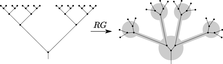
Figure 1: The RG transformation on a tree changes the connectivity of a block. One goes from $K_{0}$ (in the drawing $K_{0}=2$) to $K_{0}^{L}$ when sites at distance $L$ are grouped in the same effective node. The connectivity is an important datum in Anderson localization and one needs to keep track of it in the RG.

Starting from a tree with connectivity $K_{0}$ (see Fig. 1, where $K_{0}=2$) and proceeding in the spirit of the Kadanoff decimation procedure, we group subtrees of increasing depth creating new “effective” nodes. At step $L$, due to the Cayley tree geometry, the new node will have a larger coordination number $\mathcal{D}=K(L)+1$, which coincides with the number of nodes at distance $L$ in the original bare graph. This is the main difference with the situation in finite dimensions $d$, where the geometrical datum of the connectivity is independent of the renormalization scale $L$. According to this blocking procedure, the equation for the connectivity $K(L)$ at step $L$ is simply

$$\frac{dK}{d\ln L}=K\ln K,$$ (2)

which is not entangled with the second parameter, in contrast to the Kosterlitz-Thouless RG [27, 28, 29]. This equation has the desired solution $K(L)=K_{0}^{L}$ for some constant $K_{0}$.

One of the possibilities to introduce the physically meaningful second parameter is the following. Let us focus on an initial block of one site and let us introduce the expected number of resonant sites $\psi(L)$ at distance $L$. Starting from $\psi(L)$ one can consider other relevant physical quantities, such as the fraction of resonant sites in a block $\phi(L)=\psi(L)/K(L)$ or one of the fractal dimensions $D$.

We now write an equation for the variable $\psi$. So our RG equations must have 3 fixed points; one at $\psi=0$ (localized phase), another one at $\psi=K$ (delocalized phase), and the third, corresponding to the critical point, at $\psi=O(1)$ (set $\psi=1$ for simplicity), which must be unstable for the usual reasons. Notice that, in terms of $\phi$, the critical points are $\phi=0,\,1/K,\,1$, thus encoding the important property that, in the thermodynamic limit $L\to\infty$, the unstable critical point flows to the localized phase.

We write therefore our second equation as $\frac{d\psi}{d\ln L}=\psi\ln\psi\,\gamma(K,\psi),$ and can eliminate $L$ in favour of $K$:

$$\frac{d\psi}{dK}=\frac{\psi\ln\psi}{K\ln K}\,\gamma(K,\psi).$$ (3)

We see that the function $\gamma$ must have the property that:

$$\gamma(K,\psi)\to 1\quad\mathrm{when\ }K\to\infty,\ \mathrm{for\ all\ }\psi<1,$$ (4)

which ensures that in the localized region one can have arbitrary localization length: $\psi=e^{-L/\xi}$. This, in fact, is a solution of Eq. (3) for any $\xi$, assuming $\gamma\simeq 1$. In order to fix the other properties of the function $\gamma(K,\psi)$, we need to cast the equation for $\psi$ into an equation for a numerically accessible quantity.

Intuitively, the fractal dimension is $D=d\ln\psi/d\ln K$. To extract this quantity from the numerical data there are two possible ways, which agree in the delocalized phase but disagree in the localized region. We could define $D$ in terms of the participation entropy of an eigenstate $S_{1}=-\langle\sum_{r}\varphi^{2}(r)\,\ln\varphi^{2}(r)\rangle$, and

$$D_{1}(L)=\frac{dS_{1}}{d\ln K}.$$ (5)

This definition, which has $D_{1}\geq 0$ for all $W$ and $D_{1}=0$ for $W\geq W_{c}$, is used from now on to analyze the numerical data. Alternatively, we can define $D$ in terms of the fractal dimension of typical values of eigenstates $(\varphi^{2})_{\mathrm{typ}}\sim K^{-\alpha_{0}}$, and $D_{\mathrm{typ}}=2-\alpha_{0}$ [40]. The two definitions agree in the delocalized region but in the localized region $D_{1}=0$ and $D_{\mathrm{typ}}=-1/\xi$, being $\xi$ the localization length. For the rest of the paper we will set $D=D_{1}$.

The RG equation for the fractal dimension defines a $\beta$ function

$$\frac{d\ln D}{d\ln K}=\beta_{D}(D,K),$$ (6)

where $\beta_{D}(D,K)=(\gamma-1)/\ln K$. The function $\beta_{D}(D,K)$ is the main object of our study.

We now make the central observation of the analysis presented in this paper, which we already anticipated in the Introduction and that we will show to be supported by numerical evidence (see Fig. 2), namely that the function $\beta_{D}$ can be divided into two, conceptually different pieces

$$\beta_{D}(D,K)=\beta_{0}(D)+\beta_{1}(D,K).$$ (7)

The first term $\beta_{0}(D)$ does not depend on $K$ and it is positive $\beta_{0}(D)\geq 0$, vanishing for $D\leq 0$ and $D=1$. It can be extracted from the numerical data in Fig. 2 as we now explain. The second term is always negative for any finite system size, but it vanishes when $K\to\infty$: i.e. $\beta_{1}(D,K)<0$ for all $D,K$, $\beta_{1}(D,K)\to 0$ when $K\to\infty$. This gives us a way to extract the envelope function $\beta_{0}(D)$ from the numerically provided function $\beta_{D}(D,K)$: for fixed $D$, i.e. along vertical lines in Fig. 2, we take the maximum over $K$

$$\beta_{0}(D)=\max_{K}\beta_{D}(D,K).$$ (8)

Let us stress that the different values of $\beta_{D}(D,K)$ at different $K$ correspond to different orbits and therefore of $W$ (there is a one-to-one correspondence between $(D,K)$ and $(D,W)$). Using this prescription, putting together the numerical data for $\frac{d\ln D}{d\ln K}$ for different $W$ but with the same $K$ (system size) and $D$, and maximizing wrt $K$ we get $\beta_{0}$ as in Fig. 2. For a similar analysis on the rescaled $r$-parameter see Ref. [41]. In Fig. 5 of Ref. [41] we also show that the function $\beta_{0}(D)$ does not depend on the initial connectivity of the RRG, and thus it defines unambiguously the universality class of the Anderson model in infinite dimensions.

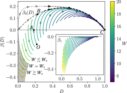
Figure 2: (Main) Numerical data for $\beta_{D}(D,K)$ (color corresponds to disorder, arrows indicate increasing system size $K$) and two possible behaviors of the function $\beta_{0}(D)$ (dashed and dotted lines). For values of $D\leq 0.3$, the curves are gray to emphasize that the shape is dependent on the fitting function used, i.e. either $\beta_{0}\propto D$ (dashed) or $\beta_{0}\propto\sqrt{D}$ (dotted). (Inset) The function $\beta_{1}(D,K)$.

Since $\beta_{1}(D,K\to\infty)=0$, the function $\beta_{0}(D)$ describes the true asymptotic limit of the RG flow and the reaching of the emergent one-parameter scaling regime. The function $\beta_{1}$ describes the evolution of the system at the beginning of the flow, before loops are encountered, and both parameters are necessary to describe the scaling. Subsequently, for sufficiently large $K$, one enters the one-parameter scaling regime:

$$\frac{d\ln D}{d\ln K}=\beta_{0}(D).$$ (9)

Our numerical data allow a reliable extraction of $\beta_{0}$ only down to $D\simeq 0.3$ so we must guess the form of $\beta_{0}$ down to $D=0$, where it must vanish. Choosing to fit the numerical data with a simple polynomial (see Ref. [41] for details) which vanishes in 0 and 1, we observe $\beta_{0}(D)=1-D+O((1-D)^{2})$ for $D\to 1$, and $\beta_{0}(D)\sim D+O(D^{2})$ for $D\to 0$, the derivatives at $D=0,1$ being 1 within the statistical error (see Fig. 2, dashed black curve). Assuming instead $\beta_{0}\sim D^{1/2}$ close to $D=0$ we get a different function (dotted curve) which deviates from the previous one in the inaccessible region $D\in[0,0.3]$. The two forms of $\beta_{0}(D)$ have different implications for what concerns the critical exponents, as discussed later.

Other functional forms of $\beta_{0}$ close to $D=0$ are also possible within our theory, but the main point of this paper stands: there exists a function $\beta_{0}(D)$, which describes the one parameter scaling flow of $D$ away from the critical point $D=0$ and towards the critical point $D=1$. This function must be calculable from first principles, but not necessarily from a Cayley tree calculation. In fact, on the Cayley tree the fractal dimension $D_{1}$ can take any value in $[0,1]$ [42, 19]. We believe the function $\beta_{0}(D)$ has not appeared in previous literature on the Anderson model on the RRG, although it is central in the discussion of finite dimensional systems [25].

The one-parameter scaling motion is the solution of the Eq. (9) obtained by integrating the differential equation by separation of variables. The result for the two different ansatzes is shown in Fig. 4 of Ref. [41]. As $\beta_{0}(D)\simeq 1-D$, as $D\to 1$ one has $\ln(1-D)\simeq\ln(K_{B}/K)$, or equivalently

$$D\simeq 1-K_{B}/K+\dots,$$ (10)

which means that the corrections satisfy volumic scaling with a critical volume $K_{B}$ to be determined in agreement with Refs. [43, 44]. In the previous expressions, $K_{B}$ is an integration constant, that corresponds to the initial condition $D_{B}$ on the single-parameter curve $\beta_{0}(D)$. Namely, $K_{B}$ is the value of $K$ at which the maximum in Eq. (8) is reached at $D=D_{B}$ (see Fig. 2). Approaching the transition at $W=W_{c}$ the value of $K_{B}$ diverges. In order to compare the curves corresponding to different $W$ (and different $K_{B}$) we shifted the curves for $D(\ln K)$ along the $\ln K$-axis so that to make them intersecting in one single point $K=K_{P}$ with $D(\ln K_{P})=0.85$ in Fig. 4 in Ref. [41] (for bare data, without collapse, see Fig. 3 in Ref. [41]). Notice that, in order to link the constant of integration $K_{B}$ to the initial conditions $K(L=L_{0}),D(L=L_{0})$, and hence to the value of disorder $W$, one needs a model of the function $\beta_{1}(K,D)$, where the initial part of the evolution occurs.

Let us also remark that the function $\beta_{1}(D,K)$ is dominant, and it has a simple form near the critical point $W_{c}=18.17$, but it becomes negligible for sufficiently large system sizes when we are far from the critical point, as it can be seen clearly in the inset of Fig. 2 that it becomes quickly zero, in correspondence of the onset of the one parameter regime.

The critical region. — In the delocalized region, the critical exponent $\nu$ is obtained by looking at the “time” $\ln(K/K(L=L_{0}))$ it takes one to reach the fixed point $D=1-\epsilon$ with any given accuracy $\epsilon\ll 1$. The approach to the fixed point $D=1$ happens in two steps: during the first one, the motion is governed by $\beta_{1}$, since $|\beta_{1}|\gg\beta_{0}$. Then, after the orbit approaches the asymptotic curve $\beta_{0}(D)$ at some value $K=K_{B}$, the motion is described by Eq. (9). Referring to the main panel of Fig. 2, we have two times to sum: the first one is the time necessary to go from the initial condition $K_{0},D(K_{0})$ till the one parameter curve $\beta_{0}(D)$, corresponding to the path $OA+AB$ in the figure. Then one moves along the $\beta_{0}$ curve till reaching the delocalized fixed point $D=1$, corresponding to the path $BC$ in the figure. The times along both $OA$ and $AB$ diverge algebraically when $W\to W_{c}$, but the corresponding exponents are different for different choices of the function $\beta_{0}(D)$ at $D\ll 1$.

Along the branch OA, when $W\to W_{c}$ from the delocalized region, we must expect according to Ref. [21] $\beta_{D}(D,K)=0$ for some value $D_{A}$ which corresponds to the minimum in the dependence $D(L)$ at a fixed $W$. As can be seen in the left panel of Fig. 7 in Ref. [41], $D_{A}$ as a function of $W$ is almost linear throughout the entire range of $W$ where the minimum is observed. In fact, a simple linear extrapolation of the fit gives $W_{c}=18.0$, a good estimate of the Anderson transition point. More specifically, the fit for $W\to W_{c}$ reads

$$D_{A}=c\,\frac{W_{c}-W}{W_{c}},\quad\mathrm{with}\quad c=1.1\pm 0.1,$$ (11)

a particularly simple result, which seems to hold mutatis mutandis for higher connectivities as well. Notice that this behavior, if continued to the localized region $W>W_{c}$, gives $D_{A}\to-1/\xi$ (using the $D_{\mathrm{typ}}$ definition), and therefore $\xi\propto(W-W_{c})^{-1}$. Equation (11) is a particularly nice formula, and it is most probably the origin of the subdiffusion observed in several numerical works [45, 46].

Since $\beta_{D}$ is proportional to the derivative $dD/d\ln K$ this means that close to the minimal value $D_{A}$ at a given $W$, the function $\beta_{D}$ has to cross the $D$ axis with infinite derivative. The simplest ansatz that describes this is a polynomial in the square root $D-D_{A}$: $\beta_{1}(D,K)=-\sqrt{D-D_{A}}(a_{0}+a_{1}(D-D_{A})^{1/2}+a_{2}(D-D_{A})^{1}+a_{3}(D-D_{A})^{3/2}...)$. This is in fact a good fit function for the data close to the critical point with $a_{0}\simeq 1$.

The time to reach the point $D=D_{A}$ (from the region $D>D_{A}$) can then be found from the solution of the equation:

$$\frac{d\ln D}{d\ln K}=-\sqrt{D-D_{A}},$$ (12)

which is

$$D(\ln K)=D_{A}\left(1+\tan\left(\frac{1}{2}\sqrt{D_{A}}\ln(K_{A}/K)\right)^{2}\right).$$ (13)

This equation can be extended from $K<K_{A}$ to $K>K_{A}$, where $\beta_{D}>0$, and it describes the motion through the minimum of $D$ as a function of $\ln K$. Now we can compute the time $\ln(K_{A}/K(L=L_{0}))$ to go from O to A, where $D_{O}=D(K(L=L_{0}))\sim O(1)$ with $D_{A}\to 0$. We find $\ln(K_{A}/K(L=L_{0}))=\pi D_{A}^{-1/2}\sim(1-W/W_{c})^{-1/2}$. If this were the only divergent timescale in the motion from the point O to the final region close to $D=1$ the critical exponent would be $\nu=1/2$ (cf. Eq. (10)). However, we now encounter two possibilities depending on the behavior of the function $\beta_{0}(D)$ close to $D=0$, one of which can introduce a new critical exponent.

1) First scenario: $\beta_{0}(D)\propto D$. There are some reasons to prefer this scenario, both based on the simplicity of the fit and on considerations of the $d\to\infty$ limit of a $d$-dimensional cube which will be subject of future work. In this case, the motion from $A$ to $B$ (see Fig. 2) intercepts $\beta_{0}$ at $D\sim D_{A}$. Since $\beta_{0}(D)\sim D$, Eq. (9) gives that the motion from $B$ to any $D=O(1)\gg D_{A}$ takes time $\ln(K_{B}/K)\propto D_{A}^{-1}$. As $D_{A}\to 0$, this time becomes dominant with respect to the time to reach the point $A$. Therefore we will have again a volume scaling of the corrections but now $D=1-e^{c(W_{c}-W)^{-1}}/K$ which corresponds to $\nu=1$.

2) Second scenario: $\beta_{0}(D)\propto D^{1/2}$. This scenario is also possible in our theory, and the present numerical results cannot exclude it. There are also reasons to favor this scenario, since in this case, the curve $\beta_{1}$ smoothly crosses over to $\beta_{0}$, no new timescale is generated, and close to ergodicity $D=1-e^{c(W_{c}-W)^{-1/2}}/K+...$ which corresponds to $\nu=1/2$ [47, 14]. Figure 2 unequivocally shows that current numerical results cannot yet rule out this scenario, and further analytical and numerical work are needed to resolve the issue.

The critical line $W=W_{c}$ is well approximated by $\beta(D)=\beta_{1}(D)=-\sqrt{D}$, which implies $D(K,W=W_{c})\propto\frac{1}{(\ln K)^{2}}$. This universal law has been observed for the first time in Ref. [39] for several ensembles of expander, graphs of constant or even fluctuating connectivity. Let us mention that, in the context of RG analysis with scaling variable $K$, the behavior on the critical line corresponds to a marginally irrelevant variable since the inverse logarithmic dependence on $K$ corresponds to a critical exponent $y=0^{-}$.

Concluding the review of the physical implications of the two above scenarios, we would like to note that within the first scenario, close to the critical point there is a window $L_{1}\equiv(1-W/W_{c})^{-1/2}<L<L_{2}\equiv(1-W/W_{c})^{-1}$ in which the running fractal dimension $D(L)$ is almost unchanged and equal to $D_{A}(W)$ [39]. The existence of two critical lengths was also discussed, in a different context, in Ref. [18] and [20]. Once the system size $L$ exceeds $L_{2}$, it quickly moves to the ergodic limit $D\approx 1$. This allows us to conclude that the length for the destruction of the finite-size multifractality has critical exponent $\nu=1$. A critical length describing a similar phenomenon, and with critical exponent $\nu=1$ was introduced in Ref. [48] for the log-normal Rosenzweig-Porter random matrix model (in that paper associated to a phenomenological model for the RRG). Recent analytical developments [20, 22], in which a new field theory of localization was proposed and studied beyond the weak-coupling regime, give a picture that in many ways resembles the one presented in this paper. Further work is needed in this direction.

Conclusions. — We have presented the equations for a real space renormalization group analysis of the Anderson model on infinite dimensional graphs and applied it to the study of the fractal dimension of the eigenstates. In particular, the fact that the critical point has all the properties of the localized phase makes the RG flow close to it quite peculiar, distinguishing it from the RG flow for finite dimensions $d$ described for the first time in Ref. [25] and from a typical Wilson-Fisher fixed point. We have introduced the division of the flow into a function which is responsible of one-parameter scaling $\beta_{0}(D)$ and which describes the approach to the ergodic fixed point $D=1$, and a two-parameter scaling part $\beta_{1}(D,K)$ which describes the remaining motion, in particular close to the minimum of $D(K)$ and to the critical point $D=0$. We believe our work provides the correct perspective to look at Hamiltonians with localized critical points, among which it is believed there are many models displaying many-body localization phenomenology [49], showing that the whole beta function needs to be considered, and not only its linearization close to the fixed point. We also provided a clean way to describe non-perturbative effects in such systems, which go beyond the tree-geometry results. Among directions for future work, let us mention finally the possibility of doing a controlled $1/d$ expansion of the Anderson model around the mean-field $d=\infty$ result discussed in this paper.

I Supplemental material - Renormalization Group Analysis of the Anderson Model on Random Regular Graphs

I.1 Data analysis for the fractal dimension

As mentioned in the main text, the numerical data for the fractal dimension are extracted from the participation entropy, defined as

$$S_{q}=\Big{\langle}\frac{1}{1-q}\sum_{i=1}^{K}\log_{2}|\varphi(i)|^{2q}\Big{\rangle},$$ (14)

and in particular, in this work, we used $S_{q}$ for $q\to 1$, which is the von Neumann entropy

$$S_{1}=-\Big{\langle}\sum_{i=1}^{K}|\varphi(i)|^{2}\log_{2}|\varphi(i)|^{2}\Big{\rangle}.$$ (15)

From $S_{1}$, the fractal dimension can be extracted as $D(L)=dS_{1}/dL$ (or equivalently as the $S_{1}(L)=D(L)L+c(L)$ [39]). We have absorbed here the $\ln K_{0}=\ln 2$ factor in the definition of $S_{q}$. Having at our disposal finite increments in the system size $L$, we computed the fractal dimension as

$$D(L)=S_{1}(L+1)-S_{1}(L)$$ (16)

and we then consider, for the numerical analysis, $\overline{D}(L+1/2)=(D(L+1)+D(L))/2$.

In order to obtain continuous curves, we interpolated the numerical values of $\overline{D}(\ln K)$ with two different fits, depending on the value of $W$. Denoting $\ln K=x$ for brevity, we use a Padé-like function for the fit at $W\leq 17$

$$f(x)=\frac{x^{3}+c_{1}x^{2}+c_{2}x+c_{3}}{x^{3}+d_{1}x^{2}+d_{2}x+d_{3}},$$ (17)

so that $f(x)=1$ for $x\to\infty$, as it should in the delocalized phase. For larger values of $W$ instead, we use a fourth-order polynomial fit in $1/x$, that perfectly fits the numerical data. We use these functions to compute the $\beta$-function using the definition and to produce the plot in Fig. 2 of the Letter, employing only the range of system sizes for which we have numerical data so that we are just interpolating, without extrapolations.

We then used these data also to determine two possible forms for the function $\beta_{0}$. The function $\beta_{0}$ has to fit the envelope that the numerical data are generating for $D\gtrsim 0.3$, and we numerically do so by fitting the set of points that are obtained by considering, for any small interval $dD$ ($D\geq 0.3$), the maximum value of $\beta(D,K)$ for all $W$. We use two different fitting functions, having different behaviors in $D=0$. The dashed line in Fig. 2 is obtained through

$$g(x)=a_{1}\,x(1-x)+a_{2}\,x(1-x)^{2}+a_{3}\,x(1-x)^{3}+a_{4}\,x^{2}(1-x)+a_{5}\,x^{2}(1-x)^{2}+a_{6}\,x^{3}(1-x),$$ (18)

while the dotted line is obtained using the fitting function

$$h(x)=b_{1}\,\sqrt{x}(1-x)+b_{2}\,\sqrt{x}(1-x)^{2}+b_{3}\,x(1-x)+b_{4}\,x^{3/2}(1-x).$$ (19)

We report the fitting coefficients in Tab. 1, and the resulting interpolations compared with the bare data in Fig. 3

$g(x)$		$h(x)$
$a_{1}$	0.153	$b_{1}$	0.986
$a_{2}$	0.235	$b_{2}$	0.266
$a_{3}$	0.476	$b_{3}$	2.517
$a_{4}$	0.285	$b_{4}$	2.429
$a_{5}$	0.366
$a_{6}$	0.501

Table 1: Fit coefficients for the functions $g(x)$ (Eq. (18)) and $h(x)$ (Eq. (19))

Figure 3: Numerical data of the fractal dimension as a function of $K$ (dots) and their interpolation using Eq. (18) and (19).

Figure 4: The function $D(\ln K)$ in the one-parameter scaling regime, for two best fits for $\beta_{0}$, the one vanishing linearly in $D=0$ (solid) and the one with square root singularity at the origin (dotted). The integration constant $K_{P}$ is chosen in such a way that all the curves intersect in one point $K=K_{P}$, where $D(K_{P})=0.85$ for all curves, numerical and analytical. The numerical data are shown as thin colored lines for $W\in[7,13]$.

Let us remark that the function $\beta_{0}$ obtained using the fitting function $g(x)$ in Eq. (18) turns out to have the symmetry $D\to 1-D$ within the precision of the fit even if $g(x)$ doesn’t have such symmetry.

I.2 $\beta$-function for the $r$-parameter

The same analysis performed on the fractal dimension can be reproduced for the $r$-parameter, once rescaled so that it ranges between $0$ and $1$ as

$$\phi=\frac{r-r_{P}}{r_{WD}-r_{P}},$$ (20)

where $r_{P}\simeq 0.386$ and $r_{WD}\simeq 0.5307$. The same procedure outlined above for the fractal dimension $D$ is applied to the data for the $r$-parameter, and the resulting $\beta$-function is displayed in the left panel of Fig. 5.

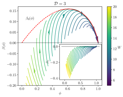
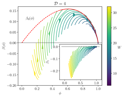
Figure 5: (Left) $\beta$-function for $\phi$, i.e. the rescaled $r$-parameter. The data analysis performed is the same that has been done for the fractal dimension. The red curve is obtained by fitting the envelope with the function $z(x)=-a(1-x)\ln(1-x)+bx(1-x)+cx^{2}(1-x)$ ($a\simeq 0.43$, $b\simeq 0.06$, $c\simeq-0.11$). In particular, the $\beta$-function approaches $\phi=1$ with an infinite derivative, as it is also confirmed by the right panel. For $\phi<0.5$ we just extrapolated the fitting function used for the points at $\phi>0.5$, and therefore can be not accurate given the limits of the numerics. (Right) Same analysis performed for a RRG with $\mathcal{D}=4$. The $\beta_{0}(D)$ function is the same as in the $\mathcal{D}=3$ case, and it is in perfect agreement with the data, supporting the universality of the function $\beta_{0}$.

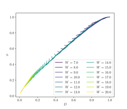
Figure 6: $\phi$ vs $D$. For intermediate values of $D$ (and $\phi$), the two quantities are almost perfectly proportional one to the other. Near $D,\phi\sim 1$ however, the curve has a vanishing derivative.

Let us mention that near $\phi=1$ the envelope of the functions $\beta(\phi)$ is different from $\beta_{0}(D)$ and, in particular, a best fit is obtained assuming that the derivative $\beta^{\prime}(\phi\to 1)$ diverges logarithmically. This gives a qualitative approach $\phi\to 1$

$$\phi\simeq 1-e^{-(K/K_{0})^{a}},$$ (21)

with $a=0.43\simeq 1/2$. Such difference is still explained in the one-parameter scaling, and it originates from the non-linear dependence of $\phi$ on $D$ (or vice-versa) near $D,\phi=1$, when plotted together as in Fig. 6. We leave a more detailed analysis of these features for future work.

We report in Fig. 7 the values of $\phi_{A}$ such that $\beta(\phi_{A})=0$, as we did for the fractal dimension. Also in this case a linear fit gives a good prediction for the critical value of the disorder. Moreover, the critical behavior of the $\beta_{1}(\phi)\sim-\sqrt{\phi}$ implies that

$$\phi_{c}(K)\propto\frac{1}{(\ln K)^{2}},$$ (22)

which has been already observed in [39]. We report in Fig. 8 the plot presented in [39], showing the $1/L^{2}$ approach to $r_{P}$ of the $r$-parameter, which turns out to be universal for many models of random graphs.

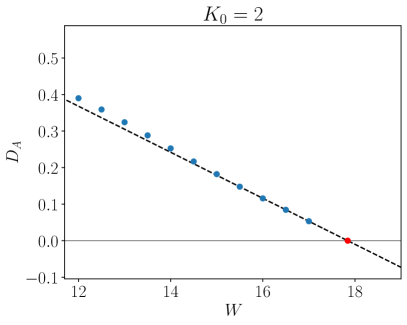
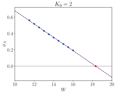
Figure 7: Values of $\phi_{A}$, i.e. the values of the rescaled $r$-parameter such that $\beta(\phi_{A})=0$, for different values of $W$ (blue dots). A linear extrapolation gives a critical value for the disorder $W_{c}=18.3\pm 0.1$ (red dot), which is in very good agreement with the known position of the transition $W_{c}=18.17$.

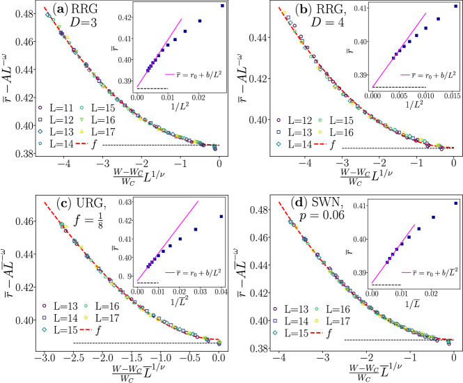
Figure 8: Figure taken from Ref. [39]. The main figures show the collapse of the $r$-parameter for different values of $W$ and system size. The collapse is obtained by setting $\omega=2$ and $\nu=1$ (see [39] for a description of the critical exponents and data collapse). The insets show the behavior of the average gap ratio at the critical point, displaying a $1/L^{2}$ scaling, which is predicted by our renormalization group equations. Different subfigures ((a), (b), (c), and (d)) correspond to different types of network, respectively RRGs with $K_{0}=2$, $K_{0}=3$, uniform random networks and small-world networks (notice that here $D$ in the plots is the vertex coordination number $K_{0}+1$).