Scalable Neural Contextual Bandit for Recommender Systems

Abstract.

High-quality recommender systems ought to deliver both innovative and relevant content through effective and exploratory interactions with users. Yet, supervised learning-based neural networks, which form the backbone of many existing recommender systems, only leverage recognized user interests, falling short when it comes to efficiently uncovering unknown user preferences. While there has been some progress with neural contextual bandit algorithms towards enabling online exploration through neural networks, their onerous computational demands hinder widespread adoption in real-world recommender systems. In this work, we propose a scalable sample-efficient neural contextual bandit algorithm for recommender systems. To do this, we design an epistemic neural network architecture, Epistemic Neural Recommendation (ENR), that enables Thompson sampling at a large scale. In two distinct large-scale experiments with real-world tasks, ENR significantly boosts click-through rates and user ratings by at least $9\%$ and $6\%$ respectively compared to state-of-the-art neural contextual bandit algorithms. Furthermore, it achieves equivalent performance with at least $29\%$ fewer user interactions compared to the best-performing baseline algorithm. Remarkably, while accomplishing these improvements, ENR demands orders of magnitude fewer computational resources than neural contextual bandit baseline algorithms.

1. Introduction

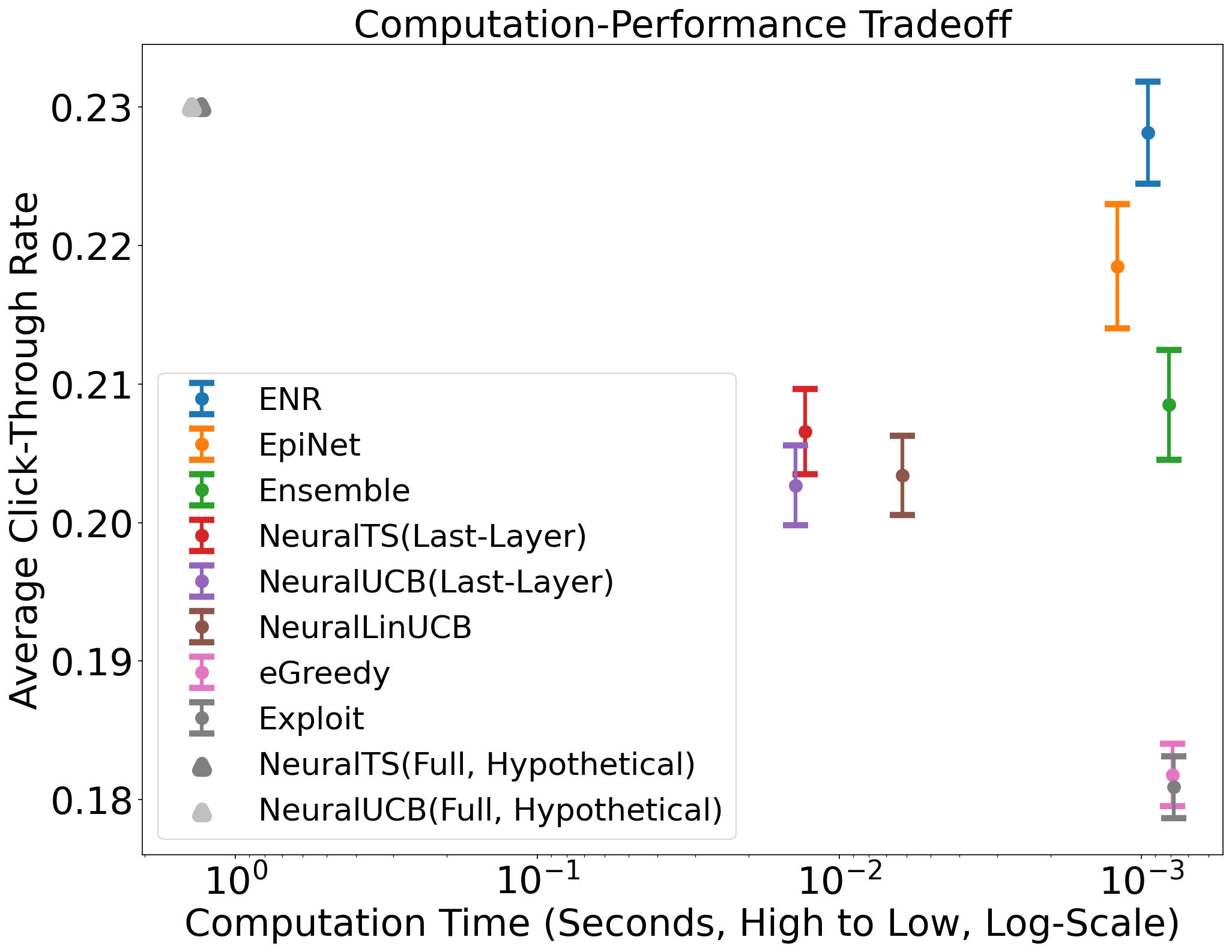
Figure 1. MIND Experiment Computation-Performance Tradeoff. Better Tradeoff towards Top Right. We expect full-scale NeuralUCB and NeuralTS to perform similarly to our methods, but require orders of magnitude more compute.

Recommender systems (RS), paramount in personalizing digital content, critically influence the quality of information accessed via the Internet. Traditionally, these systems have employed supervised learning algorithms, such as Collaborative Filtering (Resnick et al., 1994), which have greatly benefited from advances in deep learning. These algorithms analyze vast quantities of data to discern user preferences; however, they are not designed to strategically probe in order to more quickly learn about user interests. Instead, they learn passively from collected data.

Current research (Jiang et al., 2019; Salamó et al., 2005; Gravino et al., 2019) reveals that deep-learning-driven RS tend to quickly confine their focus to a limited set of suboptimal topics, limiting their scope and hampering their learning capacity. This restrictive personalization strategy confines RS to recommend only those topics with which they have established familiarity, thus failing to discover and learn users’ other potential interests. The ability of an RS to identify and learn about user’s unexplored interests is a significant determinant of its long-term performance.

The concept of exploration in RS draws heavily from bandit learning (Slivkins et al., 2019). In the bandit learning formulation of RS, the system functions as an agent, each user represents a unique context, and each recommendation is an action. Bandit learning algorithms, such as upper confidence bound (UCB) (Agrawal, 1995; Auer et al., 2002) and Thompson sampling (Thompson, 1933), provide the groundwork for efficient exploration. Theoretical advances (Agrawal and Goyal, 2012; Dong and Van Roy, 2018; Dong et al., 2019; Auer, 2002; Agrawal, 1995; Auer et al., 2002) have offered great insight into these methods, and the efficacy of such methods has been demonstrated through experiments with small-scale environments. While much of this literature has focused on small-scale environments that do not require that an agent generalizes across contexts and actions, the scale of practical RS calls for such generalization.

Advances in neural bandits offer flexible and scalable approaches to generalization that support more sample-efficient exploration algorithms. Building on ideas developed for linear UCB and linear Thompson sampling (Li et al., 2010; Chapelle and Li, 2011), these approaches offer variations of UCB and Thompson sampling that interoperate with deep learning (Li et al., 2010; Zhou et al., 2020; Xu et al., 2021; Abeille and Lazaric, 2017; Zhang et al., 2021; Lu and Van Roy, 2017; Dwaracherla et al., 2019; Osband et al., 2012; Qin et al., 2012). While these approaches may be sample-efficient, their computational requirements become onerous at scale. This has limited their practical impact.

An obstacle to scaling aforementioned approaches has been in the computation required to maintain and apply epistemic uncertainty estimates. Such estimates allow an agent to know what it does not know, which is critical for guiding exploration. The EpiNet (Osband et al., 2021) offers a scalable approach to uncertainty estimation, and therefore, a path toward supporting efficient exploration in practical RS. In particular, epinet-enhanced deep learning combined with Thompson sampling, has the potential to greatly improve RS’ exploration capabilities and therefore improve personalization. To this end, we introduce Epistemic Neural Recommendation (ENR), a novel architecture customized for RS. We run a series of experiments using large-scale real-world RS datasets to empirically demonstrate that ENR outperforms state-of-the-art neural contextual bandit algorithms. ENR greatly enhances personalization, achieving an $9\%$ and $6\%$ improvement in click-through rate and user rating, respectively, across two real-world experiments. Furthermore, it attains the performance of the best baseline algorithm with at least $29\%$ fewer user interactions. Importantly, ENR accomplishes these while requiring orders of magnitude fewer computational resources than neural contextual bandit baseline algorithms, making it a considerably more scalable solution. As a spoiler, please see Figure 1 for a computation-performance tradeoff comparison between our method and baseline methods based on one of our real-world experiments.

The remainder of this paper is organized as follows. In Section 2, we formulate RS as a contextual bandit. In Section 3, we review existing online contextual bandit algorithms, current industry adoptions, and their relative merits. In Section 4, we introduce Epistemic Neural Recommendation. In Section 5, we present empirical results. In Section 6, we summarize our contributions, benefits they afford, and potential future directions for neural contextual bandits.

2. Problem Definition

We conceptualize the design of RS as a contextual bandit problem where an agent interacts with a RS environment by taking an action (recommendation) based on a context (user) observed. More formally, the environment $\mathcal{E}$ is specified by a triple that consists of an observation space $\mathcal{O}$, an action space $\mathcal{A}$, and an observation probability function $P_{O}$.

Observation space $\mathcal{O}$: In a contextual bandit problem, the observation generated by the environment offers feedback in response to the previous action taken by the agent as well as a new context the agent needs to execute an action. Formally, $\mathcal{O}=\mathcal{S}\times\mathbb{R}$ and at time step $t$, $O_{t}=(S_{t},R_{t})$. $S_{t}\in\mathcal{S}$ is a new context. This context could, for example, provide a user’s demographic information as well as data from their past interactions. We will sometimes refer to $S_{t}$ as a user, since we think of it as providing information that distinguishes users. $R_{t}\in\mathbb{R}$ denotes scalar feedback from the user of the previous time step $t-1$ in response to the action $A_{t-1}$. For example, $R_{t}$ could be binary-valued, indicating whether the user clicked in response to a recommendation. We will refer to $R_{t}$ as the reward received by the agent at time $t$.

Action space $\mathcal{A}$: At each time $t$, the agent selects an action $A_{t}\in\mathcal{A}$, which identifies a content unit for recommendation to the user $S_{t}$. The action space $\mathcal{A}$ specifies the range of possibilities afforded by the universe of available content.

Observation probability function $P_{O}$: The observation probability function assigns a probability $P_{O}(O_{t+1}|S_{t},A_{t})$ to each possible outcome $O_{t+1}=(S_{t+1},R_{t+1})$ from recommending $A_{t}$ to user $S_{t}$. This probability is a product of two others, specified by functions $P_{S}$ and $P_{R}$:

(1) $$P_{O}(O_{t+1}|S_{t},A_{t})=P_{S}(S_{t+1})P_{R}(R_{t+1}|S_{t},A_{t}).\vspace{-5pt}$$

$P_{S}$ provides context probabilities, and $P_{R}$ provides reward probabilities. At time $t$, the environment samples a new user $S_{t}\sim P_{S}$. The agent then supplies a recommendation $A_{t}$, and the environment samples $R_{t+1}\sim P_{R}(\cdot|S_{t},A_{t})$.

The overall objective of the agent is to maximize its average reward $\frac{1}{T}\sum^{T}_{t=1}R_{t}$ over $T$ time steps. Note that, though each action $A_{t}$ does not directly impact any user other than $S_{t}$, the action influences what information is gathered through the observation $R_{t+1}$. As such, the action bears an indirect impact on subequent users through what the agent learns, which can improve its ability to make useful recommendations. Optimizing the delayed benefits of learning requires strategic sequential decisions that balance exploration versus exploitation.

We think of $S_{t}$ and $A_{t}$ as offering information about users and content units in arbitrary raw formats. Agents, however, often rely on starting with a more structured representations provided by domain experts. In this work, we also assume availability of feature extractors that map $S_{t}$ and $A_{t}$ to such representations $\phi_{A_{t}}$ and $\psi_{S_{t}}$.

Note that our problem formulation encompasses only online learning. In a real RS, one would pretrain an agent offline on historical data before engaging in online learning. The methods we develop for online learning can be applied in this workflow post pretraining of an epinet-enhanced model. However, in order to focus our attention on the problem of exploration, in this paper, we limit our discussions, designs and experiments to the online learning part and leave offline learning for future work.

3. Related Work and Prerequisites

Among various bandit algorithms, there are two most commonly adopted online bandit strategies. One explores based on the reward estimates sampled from context-action pairs’ posterior distributions, represented by Thompson sampling (Thompson, 1933), and the other follows the ”optimism in the face of uncertainty” principle, represented by upper confidence bound (UCB) (Agrawal, 1995; Auer et al., 2002). In this section, we offer a high level introduction to Thompson sampling and UCB algorithms as well as their extensions to contextual settings. Their deep neural network versions of the algorithms are considered baselines for our work. We will also review related industry and practical adoptions of these strategies. Note that in this section, we limit our discussion to exploration strategy for immediate reward and do not cover optimization approaches for cumulative returns (Zhu and Van Roy, 2023; Xu et al., 2023; Chen, 2021).

3.1. Thompson Sampling, Its Extensions and Related Adoptions

Thompson sampling is an exploration strategy that samples reward estimates from context-action pairs’ posterior distributions and then executes greedily with respect to these samples. This strategy is particularly popular due to its simplicity. Following the definition in Section 2, we first consider a vanilla Thompson sampling algorithm (Thompson, 1933) for multi-armed bandits. For a multi-armed bandit, the context $S_{t}$ is always the same and the agent needs to choose $A_{t}$ from $\mathcal{A}$ without any representation learning. A Thompson sampling agent keeps a reward posterior distribution $\hat{P}_{a}$ for each arm $a$ and updates it over time. At time step $t$, the agent chooses

(2) $$A_{t}=\arg\max_{a\in\mathcal{A}}\hat{R}_{t+1,a},\qquad\hat{R}_{t+1,a}\sim\hat{P}_{a},$$

where $\hat{R}_{t,a}$ is the estimated reward sampled from the agent’s posterior belief. The agent then updates its posterior belief $\hat{P}_{a}$ with the latest reward $R_{t+1}$ and selected action $A_{t}$. The vanilla Thompson sampling approach is a popular production strategy when it comes to small action space recommendations (Sanz-Cruzado et al., 2019; Hsieh et al., 2015).

Extending Thompson sampling to large action space and contextual bandits, an agent can compute parametric estimates of rewards of context-action pairs by sampling linear model parameters from the posterior belief (Abeille and Lazaric, 2017; Agrawal and Goyal, 2013; Russo and Van Roy, 2013, 2014; Russo et al., 2018) instead of sampling a point estimate from the reward posterior distribution. Here, a linear Thompson sampling agent keeps track of a posterior belief $\hat{P}_{\theta}$ over the parameters $\theta$. The agent chooses action

(3) $$A_{t}=\arg\max_{a\in\mathcal{A}}\hat{\theta}_{t}^{\top}x_{t,a},\qquad\hat{\theta}_{t}\sim\hat{P}_{\theta},x_{t,a}=\text{concat}(\psi_{S_{t}},\phi_{a}).$$

The agent then updates its posterior belief of $\hat{P}_{\theta}$ with the latest reward $R_{t+1}$, context $S_{t}$ and action $A_{t}$. The posterior update could be performed via Laplace approximation (Laplace, 1986), and is also presented in industry adoptions of linear Thompson sampling (Chapelle and Li, 2011).

The method above could be extended to neural networks as the agent can also keep a posterior belief over neural network parameters. To avoid heavy computation of Laplace approximation, various Bayesian methods have been proposed to achieve posterior updates for distributions over neural network parameters, including deep ensemble (Lakshminarayanan et al., 2017), ensemble sampling with prior networks (Lu and Van Roy, 2017), Bayes by Backprop (Blundell et al., 2015), Hypermodels (Dwaracherla et al., 2019), Monte-Carlo Dropouts (Gal and Ghahramani, 2016) and EpiNet (Osband et al., 2021). Among the methods above, the two ensemble methods (Brodén et al., 2018; Lu et al., 2018; Tang et al., 2014) and Monte-Carlo Dropout (Guo et al., 2020) are the most commonly adopted methods for contextual bandits with parameter posterior sampling in a practical setting.

One additional line of work that leverages Thompson sampling for neural networks is neural Thompson sampling (Zhang et al., 2021). In this approach, instead of sampling from parameters’ posterior distribution, neural Thompson sampling directly samples from the posterior estimate of the reward of a context-action pair. A Neural Thompson sampling agent keeps track of a matrix $\Gamma$ initialized with $\Gamma=\lambda\mathbf{I}$, $\mathbf{I}\in\mathbb{R}^{N\times N}$ is an identity matrix, where $\lambda>0$ is a regularization parameter and $N$ is the parameter size of the neural network. Assuming a Gaussian distributed reward posterior, the variance of the distribution is estimated by

(4) $$\sigma^{2}_{t,A}=\lambda g_{\theta}^{\top}(x_{t,A})\Gamma^{-1}g_{\theta}(x_{t,A}),$$

where $g_{\theta}$ is the gradient of the output with respect to $\theta$ for the entire neural network. The agent then chooses action

(5) $$A_{t}=\arg\max_{a\in\mathcal{A}}\hat{R}_{t+1,a},\qquad\hat{R}_{t,a}\sim\mathcal{N}(f_{\theta}(x_{t,a}),\alpha\sigma^{2}_{t,a}),$$

where $\alpha$ is an exploration hyperparameter and $f_{\theta}$ is the neural network. The agent updates $\Gamma\leftarrow\Gamma+g_{\theta}(x_{t,A})g_{\theta}(x_{t,A})^{\top}/m$ with $m$ being the width of the neural network, assuming all layers with the same width. To the best of the authors’ knowledge, the neural Thompson sampling strategy is not well adopted by industry due to its heavy computational complexity.

3.2. Upper Confidence Bound (UCB), Its Extensions and Related Adoptions

Upper confidence bound (UCB) is a general optimism facing uncertainty exploration strategy where the agent tends to choose actions that it has more uncertainties about. The purpose of doing so is to gather information that could help either identify the best action or eliminate bad actions. Similar to the subsection above, we first consider a vanilla UCB algorithm (Agrawal, 1995; Auer et al., 2002) for multi-armed bandits. A vanilla UCB agent selects an action $A_{t}$ by

(6) $$A_{t}=\arg\max_{a\in\mathcal{A}}\left(\frac{\sum_{\tau=1}^{t}R_{\tau+1}\mathbbm{1}(A_{\tau}=a)}{n_{t,a}}+\alpha\sqrt{\frac{\ln(t)}{n_{t,a}}}\right),$$

where $n_{t,A}=\sum_{\tau=1}^{t}\mathbbm{1}(A_{\tau}=A)$ and $\alpha\in\mathbb{R_{+}}$ is a hyperparameter. There have been multiple lines of work analyzing vanilla UCB’s impact on production recommender systems in terms of degenerating feedback loops (Jiang et al., 2019; Guo et al., 2023), modeling attritions (Ben-Porat et al., 2022) and its extension to Collaborative Filtering (Nakamura, 2015).

The immediate extension to UCB to linear bandit problems is LinUCB (Li et al., 2010; Chu et al., 2011). A LinUCB agent initializes two variables for any new action $A$ that it has never seen before, $\Gamma_{A}=\mathbf{I}_{d}$ ($d$-dimensional identity matrix) and $b_{A}=\mathbf{0}_{d\times 1}$ ($d$-dimensional zero vector), where $d$ is the linear parameter size. At time step t, given a new context representation $\psi_{S_{t}}$ and each action $\phi_{A}$, the agent concatenates the two vectors to get a context-action pair representation $x_{t,A}=\text{concat}(\psi_{S_{t}},\phi_{A})$. The agent selects action

(7) $$A_{t}=\arg\max_{a\in\mathcal{A}}\left((\Gamma^{-1}_{a}b_{a})^{\top}x_{t,a}+\alpha\sqrt{x_{t,a}^{\top}\Gamma_{a}^{-1}x_{t,a}}\right).$$

After receiving $R_{t+1}$, the agent then updates $\Gamma_{A_{t}}$ and $b_{A_{t}}$ with $\Gamma_{A_{t}}\leftarrow\Gamma_{A_{t}}+x_{t,A_{t}}x_{t,A_{t}}^{\top}$ and $b_{A_{t}}\leftarrow b_{A_{t}}+R_{t+1}x_{t,A_{t}}$. LinUCB is a popular algorithm for adoption in many industry usecases and particularly in the space of recommender systems (Li et al., 2010; Zhao et al., 2013; Qin et al., 2014; Wang et al., 2017).

With the rise of neural networks and deep learning, so comes the need for optimism based exploration neural methods. NeuralUCB (Zhou et al., 2020) and NeuralLinUCB (Xu et al., 2021) are two representing examples of such algorithms. We first introduce NeuralLinUCB as it’s a natural extension of LinUCB. Given a neural network representation, NeuralLinUCB no longer initiates a matrix $\Gamma_{A}$ for each action $A$ and instead keeps track of a single matrix $\Gamma$ initialized with $\lambda\mathbf{I}$ where $\lambda>0$ is a regularization factor and $\mathbf{I}\in\mathbb{R}^{N\times N}$ is an identity matrix. Suppose the neural network’s last layer representation is $\sigma_{\theta}(x_{t,A})\in\mathbb{R}^{N}$ and full model output $f_{\theta}(x_{t,A})\in\mathbb{R}$, the agent takes action

(8) $$A_{t}=\arg\max_{a\in\mathcal{A}}\left(f_{\theta}(x_{t,a})+\alpha\sqrt{\sigma_{\theta}(x_{t,a})^{\top}\Gamma^{-1}\sigma_{\theta}(x_{t,a})}\right),$$

with the same update for $\Gamma$ and $b$ except that now the update happens with the representation $\sigma_{\theta}(x_{t,A})$ instead of $x_{t,A}$. NeuralUCB follows the same principle as above, but replacing $\sigma_{\theta}(x_{t,A})$ with the gradients of all parameters within the neural network.

Although empirically the above neural methods, Neural Thompson sampling, Neural UCB and Neural LinUCB, have achieved good performance on synthetic datasets, their downside is that they all require inverting a square matrix with its dimension equal to either the entire neural network’s parameter size or the size of the last layer representation. Both in many cases are intractable, especially for real-world environments and complex neural networks.

4. Epistemic Neural Recommendation

In this section, we introduce a novel architecture for scalable neural contextual bandit problems, drawing inspiration from Thompson sampling and recent developments in epistemic neural networks (ENN) and EpiNet (Osband et al., 2021). As discussed in Section 3.1, the objective of a deep learning-based Thompson sampling strategy is to accurately estimate the uncertainty of a prediction, pertaining to a context-action pair, while keeping computational costs to a minimum. A significant drawback of many neural methods for Thompson sampling and UCB is their computationally expensive uncertainty estimation process, which impedes their integration into real-world environments. The primary aim of our proposed architecture and design is to address this very issue, while enhancing model performance.

4.1. Informative Neural Representation

A key aspect shared across all neural exploration methods is the generation of effective representations for context-action pairs. Within the contextual bandit framework, there are three main representation factors to consider: action representation, context representation, and the interaction between context and action.

We assume a general and unnormalized feature representation from the environment for both contexts and actions. To distill both context and action feature representation vectors, we initially feed each vector into a linear layer followed by a ReLU activation function. This is subsequently followed by a Layer Normalization (LayerNorm) layer (Ba et al., 2016). Given that raw features can contain disproportionately large values that are challenging to normalize - particularly in an online bandit setting where data continually stream in - it is crucial to employ layer normalization. This technique ensures smoother gradients, promoting stability and generalizability (Xu et al., 2019). More formally,

(9) $$\begin{split}h_{\beta_{\text{context}}}(\psi_{S_{t}})&=\text{LayerNorm}(\text{ReLU}(\beta_{\text{context}}^{\top}\psi_{S_{t}})),\\ h_{\beta_{\text{action}}}(\phi_{A})&=\text{LayerNorm}(\text{ReLU}(\beta_{\text{action}}^{\top}\phi_{A})),\end{split}$$

where $\theta_{\text{context}}\in\mathbb{R}^{d_{S}xd_{E}}$ and $\theta_{\text{action}}\in\mathbb{R}^{d_{A}xd_{E}}$ are the parameters for context and action summarization. Note that after summarization through these two layers, the outputs are of the same shape.

Having summarized and normalized representations for both action and context, we now model the interaction between these two entities. Collaborative Filtering (Resnick et al., 1994; Goldberg et al., 1992; Herlocker et al., 2000) and Matrix Factorization (Koren et al., 2009) provide intuitive models for this interaction. Inspired by these methods, we use element-wise multiplication to represent interactions,

(10) $$I(\psi_{S_{t}},\phi_{A})=h_{\beta_{\text{context}}}(\psi_{S_{t}})\odot h_{\beta_{\text{action}}}(\phi_{A}).$$

Utilizing the above three representations, we concatenate the three vectors to derive

(11) $$x_{t,A}=\text{concat}\left(h_{\beta_{\text{context}}}(\psi_{S_{t}}),h_{\beta_{\text{action}}}(\phi_{A}),I(\psi_{S_{t}},\phi_{A})\right).$$

Notably, this representation diverges from Neural Collaborative Filtering (NCF) (He et al., 2017) in two primary ways. Firstly, NCF can only manage id-listed features and it aggregates the concatenation of action and context through multi-layer perceptrons. In contrast, our approach can handle feature vectors without making any preliminary assumptions about the input feature shape or values. Secondly, we use the representations obtained through summarization for uncertainty estimation, as discussed in the following subsection. Moreover, we demonstrate in later sections through empirical studies that the direct application of NCF with uncertainty estimation yields inferior performance compared to our method.

4.2. Epistemic Neural Recommendation (ENR)

Using the representation derived above, we can now design a neural network for both point estimate and uncertainty estimation. For efficient epistemic uncertainty estimation using neural networks, we employ EpiNet (Osband et al., 2021), an auxiliary architecture for a general neural network. This architecture leverages the final layer representation of a neural network, along with an epistemic index $z$, to generate a sample from the posterior. EpiNet presents a cost-effective method for constructing ENNs, which has been demonstrated to excel in making joint predictions for classification and supervised learning tasks, while achieving strong performance in synthesized neural logistic bandits with minimal additional computational costs. However, a drawback of only utilizing the last layer representation, particularly in a contextual bandit setting, is the diminished representation power. The interactions between context and action are summarized through multi-layers perceptrons for marginal predictions, and considerable information is lost in the process. Motivated by this, we introduce Epistemic Neural Recommendation (ENR) that generates improved posterior samples via more informative representations.

The remaining architecture of ENR is comprised of three parts: a function $f_{\theta_{x}}:\mathbb{R}^{3d_{E}}\mapsto\mathbb{R}$ for marginal prediction, and two functions $g_{\sigma}$ and $g_{\sigma^{p}}$, both mapping from $\mathbb{R}^{3d_{E}}$ to $\mathbb{R}^{d_{z}}$, for uncertainty estimation. Upon extraction of $x_{t,A}$, we employ $f_{\theta_{x}}$ to make the marginal prediction via $f_{\theta_{x}}(x_{t,A})$.

In addition to $f_{\theta_{x}}$, $g_{\sigma}$ and $g_{\sigma^{p}}$ are independently initialized through Glorot Initialization (Glorot and Bengio, 2010; Bartlett et al., 2017), and $g_{\sigma^{p}}$ remains constant throughout its lifetime, thereby providing robust regularization. To initialize this segment of the network, ENR samples an epistemic index $z$ from its prior $P_{z}$, which could either be a discrete one-hot vector or a standard multivariate Gaussian sample. The sampled $z$ is then concatenated with $x_{t,A}$ and processed through both $g_{\sigma}$ and $g_{\sigma^{p}}$. Consequently, the uncertainty estimation is $(g_{\sigma}(x_{t,A},z)+g_{\sigma^{p}}(x_{t,A},z))^{\top}z$. Hence the final output of ENR is

(12) $$f_{\theta}(\psi_{S},\phi_{A},z)=f_{\theta_{x}}(x_{t,A})+(g_{\sigma}(sg[x_{t,A}],z)+g_{\sigma^{p}}(sg[x_{t,A}],z))^{\top}z,$$

where $x_{t,A}$ is defined in Equation 11, $\theta=(\theta_{x},\sigma,\sigma^{p},\beta_{\text{context}},\beta_{\text{action}})$, and $sg[\cdot]$ stops gradient flow of the parameter within the bracket. Note that, if the reward function is a binary variable, then a sigmoid would be added to the final output of $f_{\theta}(\psi_{S},\phi_{A},z)$ as neural logistic regression is a common setup in RS.

With the neural network above, an ENR Thompson sampling agent executes action

(13) $$A_{t}=\arg\max_{a\in\mathcal{A}}f_{\theta}(\psi_{S_{t}},\phi_{a},z),z\sim P_{z}.$$

After receiving reward $R_{t+1}$, then the agent can update the neural network with

(14) $$\theta\leftarrow\theta-\alpha\nabla_{\theta}\sum_{z\in\mathcal{Z}}\mathcal{L}(R_{t+1},f_{\theta}(\psi_{S_{t}},\phi_{A_{t}},z))$$

through stochastic gradient descent, where $\mathcal{Z}$ is a set of epistemic indices sampled from $P_{z}$ and $\alpha$ is the learning rate. In practice, we perform batch updates through sampling from a replay buffer and uses other more advanced optimization strategies such as ADAM (Kingma and Ba, 2015) for parameter updates. The loss function $\mathcal{L}$ here could be cross-entropy loss for neural logistic contextual bandits and mean squared error loss for contextual bandits with non-binary reward.

For the full illustration of the architecture, please refer to Figure 2. For a detailed algorithm illustration, please refer to Algorithm 1. We would like to also note that this algorithm is a full online bandit algorithm without any prior knowledge or pre-training. This algorithm can also be extended to perform offline pretraining before online interactions to reduce the amount of exploration required. We leave this for future work.

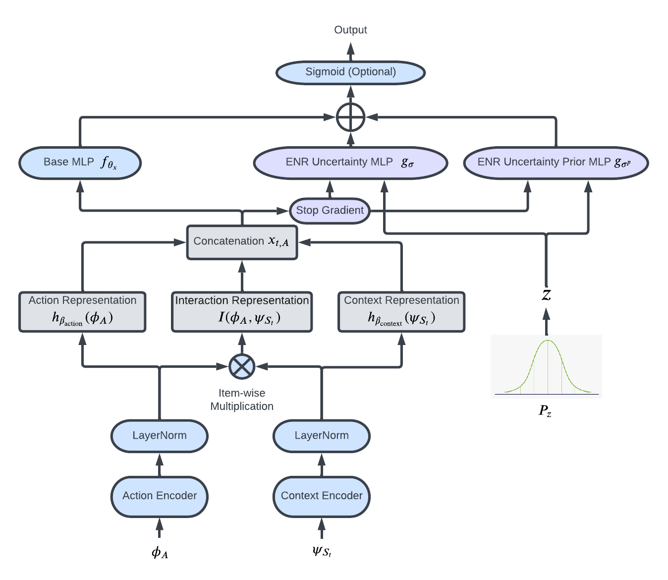
Figure 2. Epistemic Neural Recommendation Architecture

Algorithm 1 Epistemic Neural Recommendation (ENR) Thompson Sampling

1:Initialize $\theta,P_{z}$.

2:Initialize a replay buffer $\mathcal{D}$

3:for $t=1,2,\dots$ do $\triangleright$ Progressing over time steps

4:    Makes observation $O_{t}$, obtains $\psi_{S_{t}}$ and computes $R_{t}$.

5:    Store $(\psi_{S_{t-1}},\phi_{A_{t-1}},R_{t})$ in $\mathcal{D}$.

6:    Sample $z\sim P_{z}$ and compute $f_{\theta}(\psi_{S_{t}},\phi_{A},z)\forall A$ according to Equation 12.

7:    $A_{t}=\arg\max_{a\in\mathcal{A}}f_{\theta}(\psi_{S_{t}},\phi_{a},z)$.

8:    for $k=1,2,\dots,K$ do $\triangleright$ Optimization

9:         Sample a data batch $B\sim\mathcal{D}$.

10:         Sample a set of epistemic indices $Z\sim P_{z}$

11:         $\theta\leftarrow\theta-\alpha\nabla_{\theta}\sum_{i\in B}\sum_{z\in Z}\mathcal{L}(R_{i},f_{\theta}(\phi_{S_{i}},\phi_{A_{i}},z))$.

12:    end for

13:end for

5. Experiments

Table 1. Experiment Dataset Statistics

Dataset	# Users	# Items	# Interactions
MIND (Wu et al., 2020)	1,000,000	160,000	15,000,000
KuaiRec (Gao et al., 2022)	1,411	3,327	4,676,570

Table 2. MIND Dataset Illustration

Impression ID	User ID	Time	User Interest History	News with Labels
91	U397059	11/15/2019 10:22:32 AM	N106403 N71977 N97080 N102132	N129416-0 N26703-1 N120089-1 N53018-0 N89764-0

Table 3. Parameter Sizes across Different Architectures

Algorithm	MIND	KuaiRec
MLP	$0.76\times 10^{6}$	$1.21\times 10^{7}$
Wide & Deep	$/$	$2.33\times 10^{7}$
NCF	$1.51\times 10^{6}$	$2.31\times 10^{7}$
NRMS	$1.49\times 10^{6}$	$/$
NAML	$1.49\times 10^{6}$	$/$
DeepFM	$/$	$2.30\times 10^{7}$
EpiNet + MLP	$0.77\times 10^{6}$	$1.22\times 10^{7}$
EpiNet + Wide & Deep	$/$	$2.34\times 10^{7}$
EpiNet + NCF	$1.52\times 10^{6}$	$2.32\times 10^{7}$
EpiNet + NRMS	$1.50\times 10^{6}$	$/$
EpiNet + NAML	$1.50\times 10^{6}$	$/$
EpiNet + DeepFM	$/$	$2.31\times 10^{7}$
ENR	$1.52\times 10^{6}$	$2.32\times 10^{7}$

Table 4. Average Computation Time for MIND Experiments (Seconds). Both full Neural TS and Neural UCB agents require inverting a covariance matrix of approximate size $10^{6}\times 10^{6}$, which leads to $\infty$ inference time and intractable memory. Even when only using the last layer gradients, Neural TS and Neural UCB still takes about 10 times of ENR agent’s inference time.

Algorithm	Inference / Action	Training
Neural UCB (w/ any arch. below)	$\infty$	$\infty$
Neural TS (w/ any arch. below)	$\infty$	$\infty$
$\epsilon$-Greedy + MLP	$0.0006\pm 0.0001$	$0.11\pm 0.01$
Neural UCB (Last Layer) + MLP	$0.0098\pm 0.001$	$0.13\pm 0.01$
Neural LinUCB + MLP	$0.0045\pm 0.001$	$0.13\pm 0.01$
Neural TS (Last Layer) + MLP	$0.0099\pm 0.001$	$0.14\pm 0.01$
Ensemble + MLP	$0.0006\pm 0.0001$	$0.72\pm 0.03$
$\epsilon$-Greedy + NCF	$0.00079\pm 0.0001$	$0.13\pm 0.01$
Neural UCB (Last Layer) + NCF	$0.014\pm 0.002$	$0.16\pm 0.01$
Neural LinUCB + NCF	$0.0062\pm 0.001$	$0.15\pm 0.01$
Neural TS (Last Layer) + NCF	$0.013\pm 0.002$	$0.16\pm 0.01$
Ensemble + NCF	$0.00081\pm 0.0001$	$0.93\pm 0.03$
$\epsilon$-Greedy + NAML	$0.00082\pm 0.0001$	$0.13\pm 0.01$
Neural UCB (Last Layer) + NAML	$0.014\pm 0.002$	$0.15\pm 0.01$
Neural LinUCB + NAML	$0.063\pm 0.001$	$0.15\pm 0.01$
Neural TS (Last Layer) + NAML	$0.014\pm 0.002$	$0.15\pm 0.01$
Ensemble + NAML	$0.00079\pm 0.0001$	$0.95\pm 0.03$
$\epsilon$-Greedy + NRMS	$0.00083\pm 0.0001$	$0.14\pm 0.01$
Neural UCB (Last Layer) + NRMS	$0.013\pm 0.002$	$0.16\pm 0.01$
Neural LinUCB + NRMS	$0.006\pm 0.001$	$0.15\pm 0.01$
Neural TS (Last Layer) + NRMS	$0.014\pm 0.002$	$0.15\pm 0.01$
Ensemble + NRMS	$0.00078\pm 0.0001$	$0.91\pm 0.03$
EpiNet + MLP	$0.0007\pm 0.0001$	$0.12\pm 0.01$
EpiNet + NCF	$0.0012\pm 0.0001$	$0.16\pm 0.01$
EpiNet + NAML	$0.0013\pm 0.0001$	$0.17\pm 0.01$
EpiNet + NRMS	$0.0012\pm 0.0001$	$0.17\pm 0.01$
ENR	$0.00095\pm 0.0001$	$0.18\pm 0.01$

Table 5. Average Computation Time for KuaiRec Experiments (Seconds). Both full Neural TS and Neural UCB agents require inverting a covariance matrix of approximate size $10^{7}\times 10^{7}$, which leads to $\infty$ inference time and intractable memory. Note that NeuralUCB and NeuralTS agents that only compute the last layer of gradients still takes 150 times of ENR’s inference time due to available action size of 3327 for every time step, hence intractable in this experiment.

Algorithm	Inference / Action	Training
Neural UCB (w/ any arch. below)	$\infty$	$\infty$
Neural TS (w/ any arch. below)	$\infty$	$\infty$
$\epsilon$-Greedy + MLP	$0.012\pm 0.001$	$0.24\pm 0.01$
Neural UCB (Last Layer) + MLP	$1.60\pm 0.13$	$0.25\pm 0.01$
Neural LinUCB + MLP	$0.036\pm 0.002$	$0.25\pm 0.01$
Neural TS (Last Layer) + MLP	$1.59\pm 0.13$	$0.25\pm 0.01$
Ensemble + MLP	$0.018\pm 0.001$	$1.2\pm 0.03$
$\epsilon$-Greedy + NCF	$0.013\pm 0.001$	$0.31\pm 0.02$
Neural UCB (Last Layer) + NCF	$1.71\pm 0.13$	$0.35\pm 0.02$
Neural LinUCB + NCF	$0.042\pm 0.002$	$0.36\pm 0.02$
Neural TS (Last Layer) + NCF	$1.72\pm 0.13$	$0.36\pm 0.02$
Ensemble + NCF	$0.020\pm 0.001$	$1.5\pm 0.03$
$\epsilon$-Greedy + Wide & Deep	$0.013\pm 0.001$	$0.32\pm 0.02$
Neural UCB (Last Layer) + Wide & Deep	$1.68\pm 0.13$	$0.34\pm 0.02$
Neural LinUCB + Wide & Deep	$0.039\pm 0.002$	$0.35\pm 0.02$
Neural TS (Last Layer) + Wide & Deep	$1.69\pm 0.13$	$0.34\pm 0.02$
Ensemble + Wide & Deep	$0.020\pm 0.001$	$1.6\pm 0.03$
$\epsilon$-Greedy + DeepFM	$0.014\pm 0.001$	$0.32\pm 0.02$
Neural UCB (Last Layer) + DeepFM	$1.72\pm 0.13$	$0.36\pm 0.02$
Neural LinUCB + DeepFM	$0.041\pm 0.002$	$0.36\pm 0.02$
Neural TS (Last Layer) + DeepFM	$1.72\pm 0.13$	$0.36\pm 0.02$
Ensemble + DeepFM	$0.021\pm 0.001$	$1.6\pm 0.03$
EpiNet + MLP	$0.013\pm 0.001$	$0.28\pm 0.01$
EpiNet + NCF	$0.015\pm 0.001$	$0.37\pm 0.01$
EpiNet + Wide & Deep	$0.015\pm 0.001$	$0.38\pm 0.01$
EpiNet + DeepFM	$0.014\pm 0.001$	$0.38\pm 0.01$
ENR	$0.012\pm 0.001$	$0.38\pm 0.01$

In this section, we will go through a set of experiments ranging from a toy experiment to large-scale real-world data experiments. The dataset statistics are shown in Table 1. Each of the dataset has millions of interactions. We will compare ENR and EpiNet (Osband et al., 2021) (first time adopted for neural contextual bandits) against $\epsilon$-Greedy, Ensemble Sampling with Prior Networks (Ensemble) (Lu and Van Roy, 2017), Neural Thompson Sampling (Neural TS) (Zhang et al., 2021), Neural UCB (Zhou et al., 2020), and Neural LinUCB (Xu et al., 2021), each with a similar sized neural network. In addition, to assess advantages attributable to the architecture of ENR, we will also evaluate it against a few well recognized RS neural network architecture including, Neural Collaborative Filtering (NCF) (He et al., 2017), Neural Recommendation with Attentive Multi-View Learning (NAML) (Wu et al., 2019a), Neural Recommendation with Multi-Head Self-Attention (NRMS) (Wu et al., 2019b), Wide and Deep (Cheng et al., 2016), and DeepFM (Guo et al., 2017), combined with exploration strategies above. To ensure fairness of evaluation, we ensure that all neural network architectures other than vanilla MLP has a similar parameter size. See Table 3. The algorithms all adopt ADAM (Kingma and Ba, 2015) for model optimization.

Note that for both Neural UCB and Neural Thompson Sampling, due to their scalability, we are only able to experiment them with their last layer versions, where we only compute gradients of the last layer of the neural networks. The full Neural UCB and Neural Thompson Sampling agents require inverting matrices of sizes $10^{6}\times 10^{6}$ (7.45 TB of memory and $O(10^{18})$ complexity) and $10^{7}\times 10^{7}$ (745 TB of memory and $O(10^{21})$ complexity) for MIND and KuaiRec experiments respectively, which are intractable in most commercial machines. See more details of computation costs in Table 4 and 5 respectively for two experiments and all experiments are performed on an AWS p4d24xlarge machine with 8 A100 GPUs, each GPU with 40 GB of GPU memory. NeuralLinUCB requires 6x and 3.5x inference time compared to our method in two real-world experiments with a similar training time. Simplified versions of NeuralTS and NeuralUCB using only gradients from the last layer of NNs require 10x and 100x inference time compared to our method in these experiments. Lastly, Ensemble requires a similar inference time, but requires 5x training time compared to our method with parallel computing optimization. NeuralLinUCB, NeuralUCB, NeuralTS all require orders of magnitude higher inference cost and Ensemble requires orders of magnitude higher training cost.

We will use average reward as performance metric in the following experiments (average click-through rate and average user rating in MIND and KuaiRec respectively). We choose to not use classic metrics like NDCG or precision because they are supervised-learning metrics. In online bandits, the agent’s optimal strategy could try to explore and retrieve information instead of optimizing these metrics.

Table 6. Average Regret for Toy Experiments

Algorithm	Exploit	$\epsilon$-Greedy	Neural UCB	Neural LinUCB	Neural TS	Ensemble	EpiNet	ENR
Avg Regret	$0.10\pm 0.006$	$0.11\pm 0.01$	$0.11\pm 0.007$	$0.07\pm 0.009$	$0.075\pm 0.008$	$0.08\pm 0.004$	$0.064\pm 0.003$	$\mathbf{0.053\pm 0.0006}$

Table 7. User Interactions (Thousands) Needed for Best Algorithm Candidates (Selected among Different Neural Network Architectures) to Reach Standard Performance and Savings Compared to Non-EpiNet Baselines

Algorithm	Exploit	$\epsilon$-Greedy	Neural UCB	Neural LinUCB	Neural TS	Ensemble	EpiNet	ENR	Savings
MIND ($0.2$ Click-Through Rate)	$\infty$	$\infty$	$277$	$268$	$184$	$142$	$145$	62	$56\%$
KuaiRec ($2.3$ User Rating)	N/A	$4.5$	N/A	$4$	N/A	$2.4$	$2.1$	1.7	$29\%$

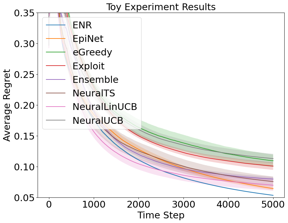
Figure 3. Toy Experiment Results

Table 8. Average Click-Through Rate for MIND Experiments

Algorithm	MIND Train	MIND Eval
Exploit + MLP	$0.170\pm 0.0007$	$0.168\pm 0.0011$
$\epsilon$-Greedy + MLP	$0.171\pm 0.0007$	$0.167\pm 0.0011$
Neural UCB (Last Layer) + MLP	$0.188\pm 0.0016$	$0.192\pm 0.0010$
Neural LinUCB + MLP	$0.189\pm 0.0032$	$0.192\pm 0.00086$
Neural TS (Last Layer) + MLP	$0.191\pm 0.0023$	$0.194\pm 0.0015$
Ensemble + MLP	$0.193\pm 0.0022$	$0.191\pm 0.0009$
Exploit + NCF	$0.181\pm 0.0022$	$0.179\pm 0.0024$
$\epsilon$-Greedy + NCF	$0.182\pm 0.0023$	$0.178\pm 0.0025$
Neural UCB (Last Layer) + NCF	$0.203\pm 0.0029$	$0.203\pm 0.0023$
Neural LinUCB + NCF	$0.203\pm 0.0029$	$0.203\pm 0.0030$
Neural TS (Last Layer) + NCF	$0.207\pm 0.0031$	$0.206\pm 0.0028$
Ensemble + NCF	$0.209\pm 0.0040$	$0.206\pm 0.0031$
Exploit + NAML	$0.180\pm 0.0021$	$0.178\pm 0.0024$
$\epsilon$-Greedy + NAML	$0.182\pm 0.0022$	$0.178\pm 0.0025$
Neural UCB (Last Layer) + NAML	$0.202\pm 0.0028$	$0.203\pm 0.0024$
Neural LinUCB + NAML	$0.203\pm 0.0028$	$0.203\pm 0.0030$
Neural TS (Last Layer) + NAML	$0.206\pm 0.003$	$0.207\pm 0.0028$
Ensemble + NAML	$0.208\pm 0.0039$	$0.206\pm 0.0031$
Exploit + NRMS	$0.181\pm 0.0022$	$0.178\pm 0.0024$
$\epsilon$-Greedy + NRMS	$0.182\pm 0.0023$	$0.178\pm 0.0025$
Neural UCB (Last Layer) + NRMS	$0.203\pm 0.0029$	$0.203\pm 0.0024$
Neural LinUCB + NRMS	$0.204\pm 0.0029$	$0.203\pm 0.0030$
Neural TS (Last Layer) + NRMS	$0.206\pm 0.0030$	$0.207\pm 0.0027$
Ensemble + NRMS	$0.208\pm 0.0039$	$0.206\pm 0.0031$
EpiNet + MLP	$0.204\pm 0.003$	$0.199\pm 0.0012$
EpiNet + NCF	$0.219\pm 0.004$	$0.214\pm 0.0028$
EpiNet + NAML	$0.217\pm 0.004$	$0.214\pm 0.0028$
EpiNet + NRMS	$0.218\pm 0.004$	$0.214\pm 0.0027$
ENR	$\mathbf{0.228\pm 0.004}$	$\mathbf{0.220\pm 0.0026}$

Table 9. Average Reward for KuaiRec Experiments

Algorithm	KuaiRec Train	KuaiRec Eval
$\epsilon$-Greedy + MLP	$1.41\pm 0.087$	$1.57\pm 0.11$
Neural LinUCB + MLP	$1.68\pm 0.15$	$1.59\pm 0.13$
Ensemble + MLP	$2.28\pm 0.061$	$2.03\pm 0.09$
$\epsilon$-Greedy + NCF	$2.42\pm 0.0075$	$2.31\pm 0.019$
Neural LinUCB + NCF	$2.47\pm 0.022$	$2.38\pm 0.020$
Ensemble + NCF	$2.55\pm 0.003$	$2.46\pm 0.005$
$\epsilon$-Greedy + Wide & Deep	$2.38\pm 0.007$	$2.27\pm 0.018$
Neural LinUCB + Wide & Deep	$2.42\pm 0.021$	$2.35\pm 0.017$
Ensemble + Wide & Deep	$2.52\pm 0.003$	$2.43\pm 0.005$
$\epsilon$-Greedy + DeepFM	$2.38\pm 0.0075$	$2.32\pm 0.022$
Neural LinUCB + DeepFM	$2.45\pm 0.022$	$2.36\pm 0.019$
Ensemble + DeepFM	$2.53\pm 0.003$	$2.47\pm 0.005$
EpiNet + MLP	$2.43\pm 0.01$	$2.17\pm 0.087$
EpiNet + NCF	$2.58\pm 0.0047$	$2.43\pm 0.016$
EpiNet + Wide & Deep	$2.56\pm 0.005$	$2.41\pm 0.018$
EpiNet + DeepFM	$2.57\pm 0.0046$	$2.46\pm 0.021$
ENR	$\mathbf{2.62\pm 0.0005}$	$\mathbf{2.63\pm 0.066}$

5.1. Toy Experiment

For this experiment, we define a synthetic environment to evaluate the performance of ENR compared to various baselines mentioned above. According to Section 2, the synthetic environment is characterized as: Both action and context vectors are of dimension 100. $R_{t+1}\sim\text{Bernoulli}\left(\sigma(\theta^{\top}\text{concat}(\psi_{S_{t}},\phi_{A_{t}}))\right)$. The size of $\mathcal{A}$ is 100. $\sigma$ is the Sigmoid function and both $\theta$ is unknown to all the agents as the learning target. All of $\theta,\phi_{A},\psi_{S}$ are sampled from standard Gaussian. Since the toy environment is synthesized, we could compute the regret of the algorithms as

(15) $$\text{Regret}(T)=\frac{1}{T}\sum_{t=1}^{T}(R_{t,A^{*}_{t}}-R_{t,A_{t}}),$$

where $R_{t,A^{*}_{t}}$ indicates the reward of the optimal action given the context $S_{t}$. In this experiment, we use a hidden layer of (200, 100) for MLP and the main neural network architecture for MLP and ENR. The action and context summarization layer for ENR is set without hidden layers and with activation of ReLU with Layer Normalization on top of that. The uncertainty estimation architecture of ENR is set with hidden layer of (50, 20). The EpiNet architecture is set to a single hidden layer of 50. All prior network scaling is set to 0.3. Dimension of epistemic indices is set to 5 for EpiNet and ENR. The results are averaged over 50 independent experiments. The experiment is run for 5000 steps.

See Figure 3 and Table 6 for more details of the experiment results. We see that ENR marginally improves on top of EpiNet with a similarly sized base neural network of fully connected layers. Given that the setups of both toy experiments are relatively simple, it is expected that sophisticated neural representations would not make material difference.

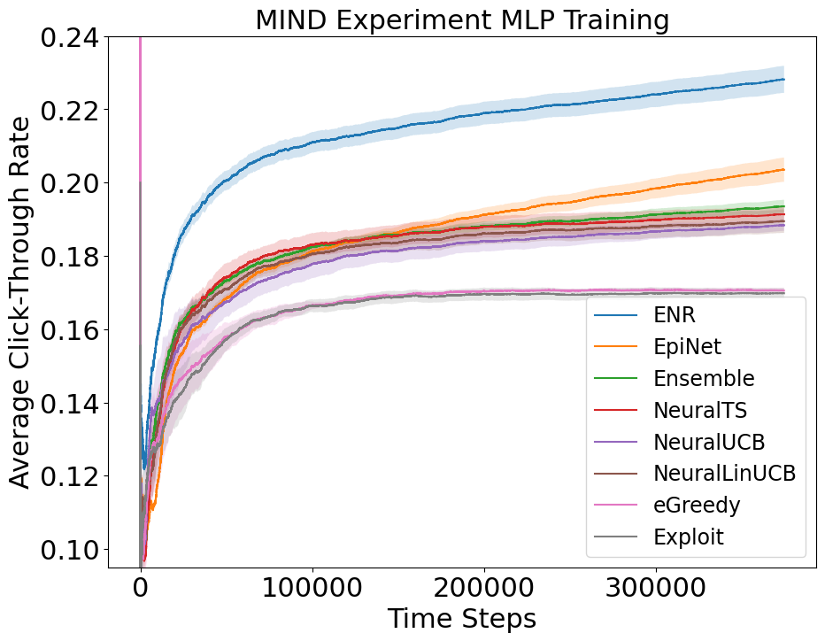
(a) MIND Experiment MLP Training Results

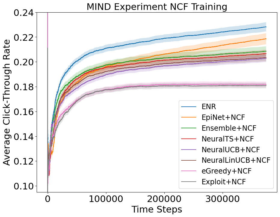
(b) MIND Experiment NCF Training Results

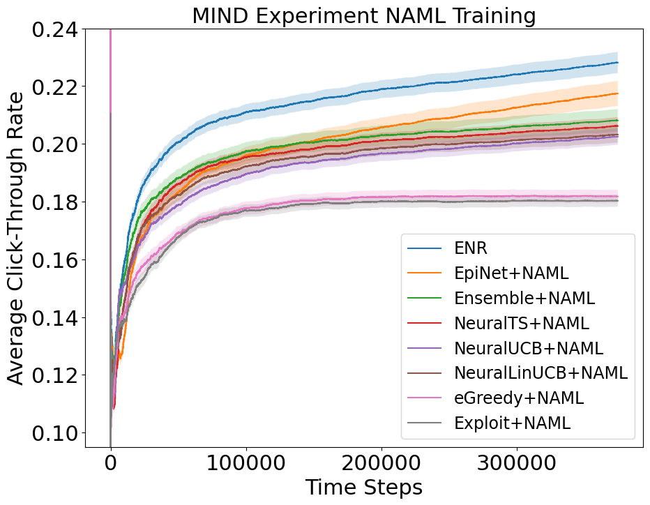
(c) MIND Experiment NAML Training Results

(d) MIND Experiment NRMS Training Results

Figure 4. MIND Experiments Contextual Bandit Training Outcome

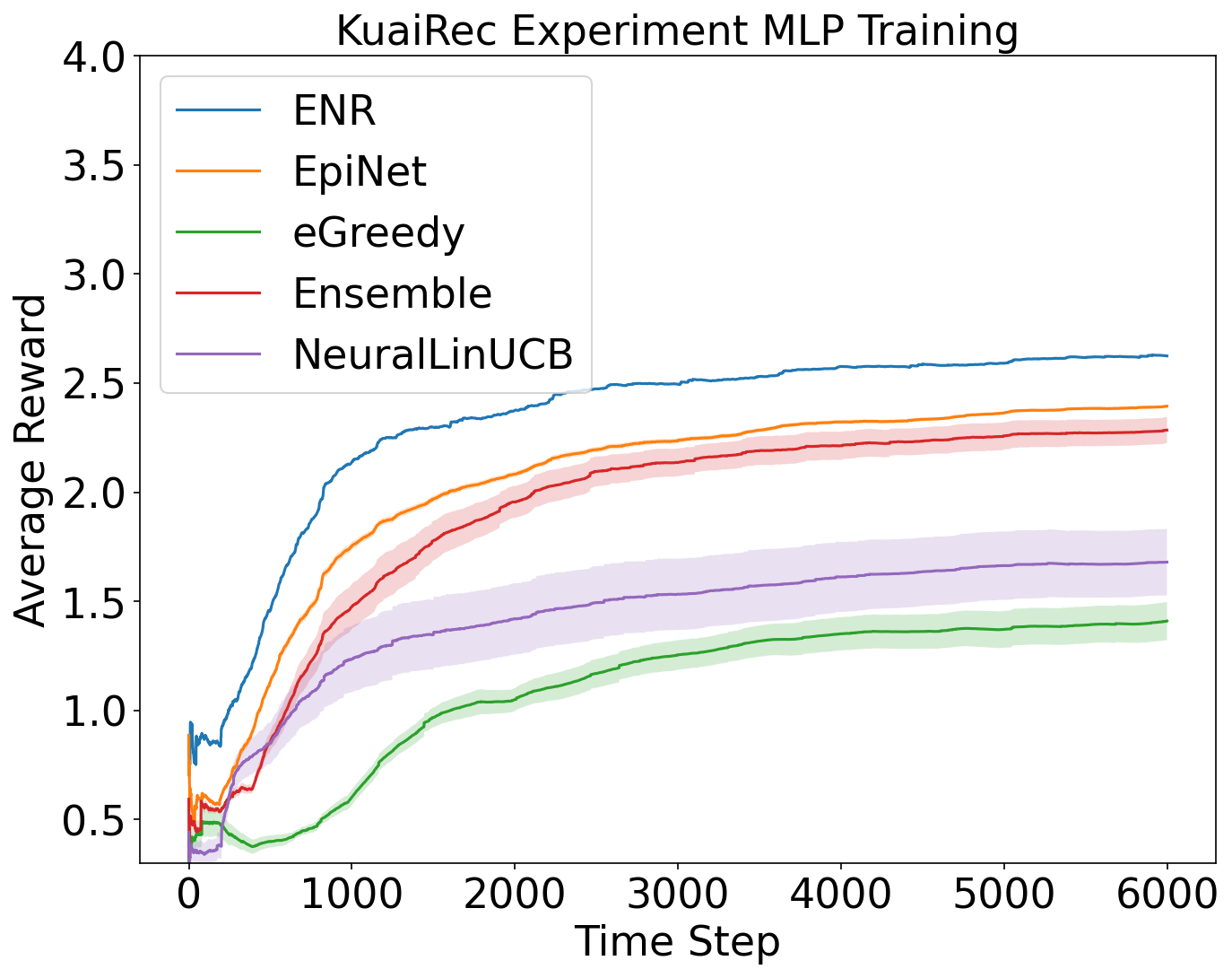
(a) KuaiRec Experiment MLP Training Results

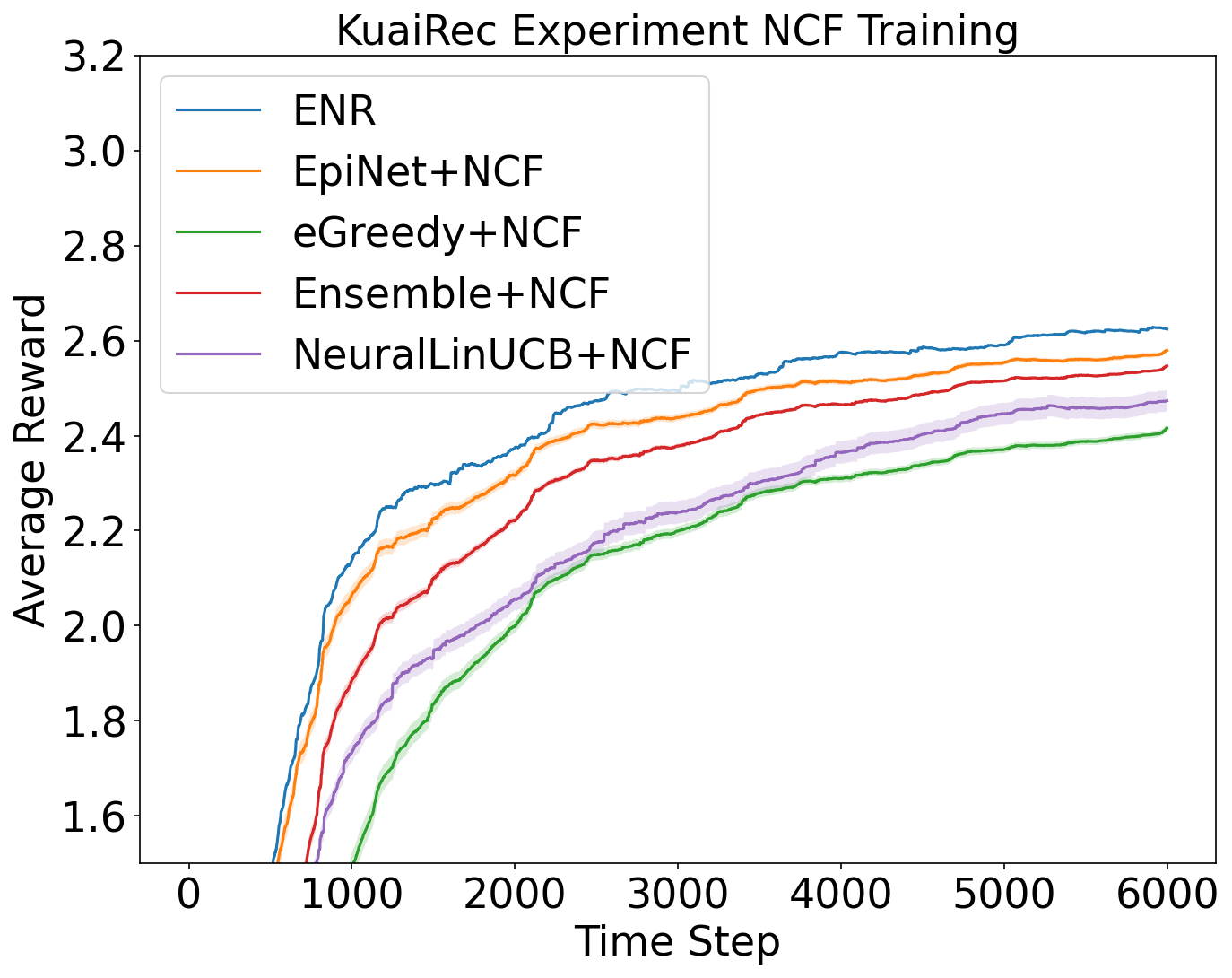
(b) KuaiRec Experiment NCF Training Results

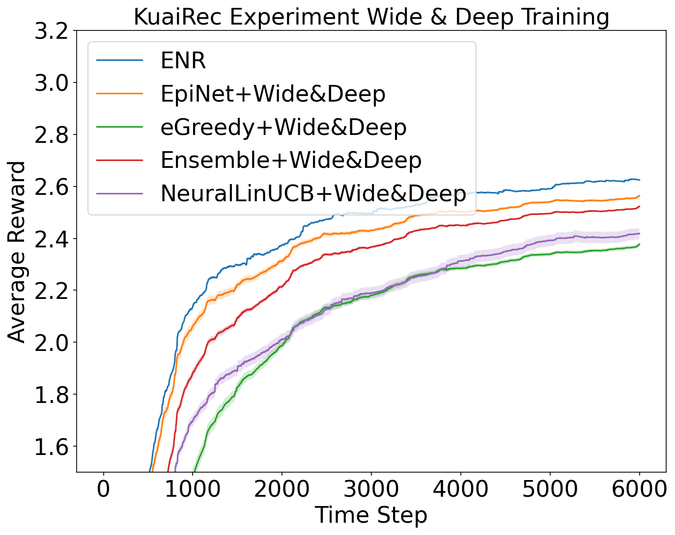
(c) KuaiRec Experiment Wide & Deep Training Results

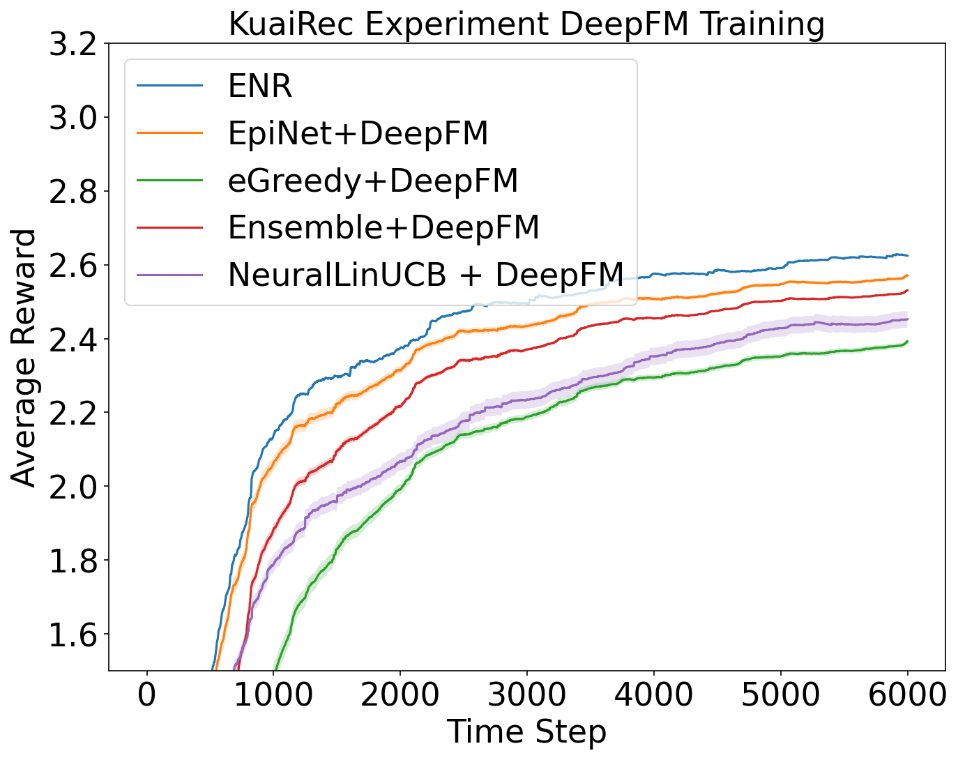
(d) KuaiRec Experiment DeepFM Training Results

Figure 5. KuaiRec Experiments Contextual Bandit Training Outcome

5.2. MIND Dataset Experiment (Wu et al., 2020)

MIND is a large-scale dataset generated by Microsoft news recommender system. It provides anonymized data logs that record each user’s historical interesting articles and their impression as well as click logs with new recommendations. The dataset contains over millions of anonymized interaction logs. For statistics of the dataset, please refer to Table 1. One unique advantage of the MIND dataset for contextual bandit setup is its complete ground truth. At time step $t$, the MIND dataset logs $K$ distinct news recommendations sent to the user and records the news articles the user gave good feedback on, all of which happen at a single timestamp. Please see Table 2 for an illustration of the data we use. Hence when evaluating the outcome of any action chosen by an agent among the sent recommendations, we can directly use the groundtruth from the dataset and avoid counterfactual evaluation which leads to high variance.

In this experiment, we use all exploration baseline strategies as well as NCF (He et al., 2017), NAML (Wu et al., 2019a) and NRMS (Wu et al., 2019b) for neural network architecture baselines. It is worth noting that in this experiment, we adopt the Multi-Head Self-Attention architecture mentioned in NRMS (Wu et al., 2019b) to extract representation for context (user) before feeding into the neural networks (except NAML where it has its own summarization module). We did not select Wide & Deep and DeepFM because both neural architectures are heavily built on sparse feature optimization, which is not present in this experiment.

In the following, we use a hidden layer of (1000, 500, 100, 50) for MLP and the final neural network architecture for NCF and ENR. NCF’s first MLP uses hidden layer of (1000, 500). For NAML and NRMS, EpiNet is added to the last layer replacing dot product with item-wise multiplication. The action and context summarization layer for ENR is set without hidden layers and with activation of ReLU and Layer Normalization on top of that. The uncertainty estimation architecture of ENR is set with hidden layer of (1000, 500). The EpiNet architecture for other neural networks are set with a single hidden layer of 50. All prior network scaling is set to 0.3. Dimension of epistemic indices is set to 5 for all EpiNets and ENR. The results are averaged over 10 independent experiments. Each training experiment is run for 375,000 time steps by sampling 375,000 users randomly from the dataset. In addition, we also sample 2,000 users that are never seen by the agent as evaluation set for out of sample evaluation.

See Figure 4 as well as Table 8 for the experiment results. ENR is able to outperform all other baselines with a big margin in both online interaction and offline out-of-sample evaluation, outperforming $9\%$ and $6\%$ respectively in Click-Through Rate compared to the best baseline candidate (excluding EpiNet candidates, as that is considered part of the contribution of this work) respectively. Moreover, ENR is able to achieve a standard performance of $0.2$ click-through rate with $56\%$ less user interactions compared to the best non-EpiNet baseline. See Table 7 for more details.

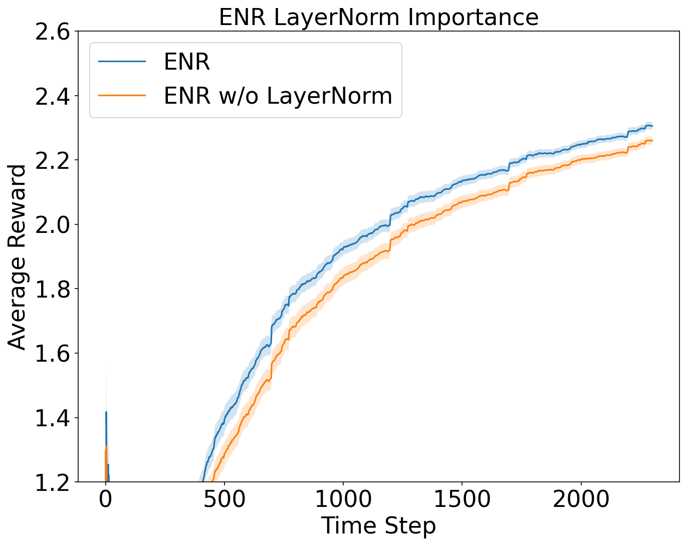
(a) Comparison between with and without Layer Normalization Based on KuaiRec

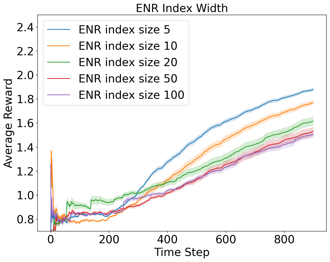
(b) Selection of Index Width Based on KuaiRec

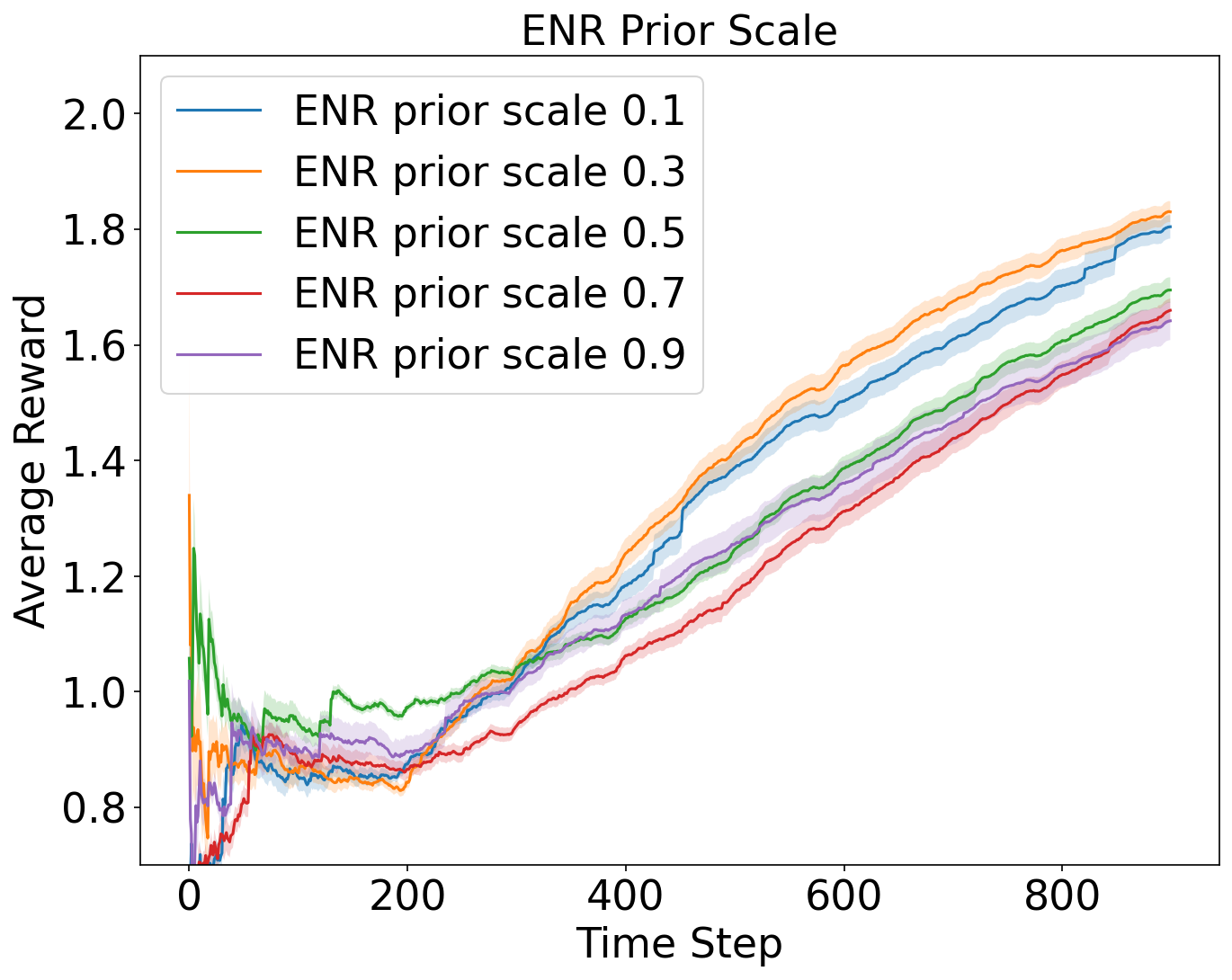
(c) Selection of Prior Scale Based on KuaiRec

Figure 6. Ablation Studies

5.3. KuaiRec Dataset Experiment (Gao et al., 2022)

The last experiment we run is through the KuaiRec dataset. KuaiRec offers almost a full dense matrix in terms of the interactions between users and actions. The density is at 99.6%. For more details of the dataset statistics, please refer to Table 1. With these characteristics of the dataset, we can evaluate all of the algorithms in real-world contextual bandit environment with huge available set of recommendations at every step without resorting to counterfactual evaluation. It is worth noting that, different from MIND, KuaiRec’s user ratings on each recommendation are collected at slightly different times, and hence present a less rigorous grounding for avoiding counterfactual evaluation. Nevertheless, we believe it is valuable to still study the performance of ENR and EpiNet algorithms when facing a huge available set of actions at every timestep. We also note that such datasets, with feedback collected at different times, are commonly used in bandit learning literature to evaluate algorithms’ performance, e.g. (Christakopoulou and Banerjee, 2018; Hong et al., 2020; Zhang et al., 2020).

In this experiment, we adopt all exploration strategies except Neural Thompson Sampling and Neural UCB due to their computation complexity. Given that both strategies requires a gradient pass on every action from the candidate list, these algorithms do not scale to a problem with 3,327 actions at every time step. We also choose NCF, Wide & Deep and DeepFM as neural network architectures given that the features provided in the dataset are raw features with many categorical features. The dataset does not provide user historical articles and hence NAML and NRMS are not good fits.

In the following, we use a hidden layer of (4096, 1024, 512, 128) for MLP and the final neural network architecture for NCF and ENR. NCF’s first MLP uses hidden layer of (1024, 512). Wide & Deep and DeepFM adopts the same hidden layer structure for dense embeddings. The action and context summarization layer for ENR is set without hidden layers and with activation of ReLU with Layer Normalization on top of that. The uncertainty estimation architecture of ENR is set with hidden layer of (1024, 128). The EpiNet architecture for other neural networks are set with a single hidden layer of 128. All prior network scaling is set to 0.3. Dimension of epistemic indices is set to 5 for all EpiNets and ENR. The results are averaged over 10 random seeds. Each experiment is run for 6,000 time steps where each context is randomly sampled from the small matrix excluding an evaluation set of 100 contexts. One unique thing to note in this dataset is that user feedback for items in this dataset are rating scalars. Therefore, we use regression and mean squared error loss instead of cross entropy loss.

See Figure 5 as well as Table 9 to see the detailed results of the experiment. From the results, we can see that ENR outperforms all other candidates in both in-sample online interactions as well as offline out-of-sample evaluation set by $4\%$ and $6\%$ respectively. Another observation we draw from the result is that with a complete action space provided to the agent at every timestep, all algorithms significantly improve in generalization capabilities from in-sample predictions to out-of-sample predictions. In Table 7, we also show that ENR requires $29\%$ less user interactions compared to the best non-EpiNet baseline to achieve a standard performance of $2.3$ average user rating.

5.4. Ablation Studies

In this section, we cover some ablation studies regarding some of our hyperparameter choices as well as some design choices.

5.4.1. The Importance of Layer Normalization

In ENR, one of a key components for action and context summarization is Layer Normalization. As ENR is designed to take in any context and action inputs, it is common to observe a few features that are outsized. To ensure that context action interaction is not dominated by a few particular features, before the item-wise multiplication, we add a Layer Normalization operator to ensure more stability in the neural network as well as getting less impacted by outliers during training. See Figure 6(a) for a performance comparison between ENR with and without Layer Normalization.

5.4.2. Selection of Epistemic Index Width

Epistemic index $z$ is the key to identify a posterior sample from an ENR, and we study the impact of index dimension in this study. See Figure 6(b). As the width of the index grows, the performance of the algorithm relatively decays. From the figure, we can also see that index width of 5 outperforms others. Hence we choose 5 for all of our experiments.

5.4.3. Selection of ENR Uncertainty Prior Network Scale

The prior network is a key means to regularize Epistemic Neural Networks by pulling the posterior distribution back from diverging too far away from the prior distribution to avoid distribution collapse. We study the prior network scale for ENR through a sweep. Note that prior scale is a scalar ranging $(0,1)$. See Figure 6(c). We see that setting prior scale to 0.3 offers the best performance.

6. Conclusion

In this paper, we designed a scalable and novel neural contextual bandit algorithm customized for recommender systems via a new epistemic neural network architecture and Thompson sampling. We formally define the recommender system problem as a contextual bandit problem and reviewed the current State-of-the-Art neural contextual bandit strategies. Our architecture design, Epistemic Neural Recommendation (ENR), presents much better scalability compared to other neural contextual bandit strategies. We show empirically through both synthetic experiments as well as two large-scale real-world experiments that ENR outperforms all other baselines. We hope that the results and the design in this paper inspires adoption of Epistemic Neural Recommendation as well as neural contextual bandit approaches in real-world systems.

References

- (1)
- Abeille and Lazaric (2017) Marc Abeille and Alessandro Lazaric. 2017. Linear Thompson sampling revisited. In Artificial Intelligence and Statistics. PMLR, 176–184.
- Agrawal (1995) Rajeev Agrawal. 1995. Sample mean based index policies by o (log n) regret for the multi-armed bandit problem. Advances in Applied Probability 27, 4 (1995), 1054–1078.
- Agrawal and Goyal (2012) Shipra Agrawal and Navin Goyal. 2012. Analysis of thompson sampling for the multi-armed bandit problem. In Conference on learning theory. JMLR Workshop and Conference Proceedings, 39–1.
- Agrawal and Goyal (2013) Shipra Agrawal and Navin Goyal. 2013. Thompson sampling for contextual bandits with linear payoffs. In International conference on machine learning. PMLR, 127–135.
- Auer (2002) Peter Auer. 2002. Using confidence bounds for exploitation-exploration trade-offs. Journal of Machine Learning Research 3, Nov (2002), 397–422.
- Auer et al. (2002) Peter Auer, Nicolo Cesa-Bianchi, and Paul Fischer. 2002. Finite-time analysis of the multiarmed bandit problem. Machine learning 47, 2 (2002), 235–256.
- Ba et al. (2016) Jimmy Lei Ba, Jamie Ryan Kiros, and Geoffrey E Hinton. 2016. Layer Normalization. stat 1050 (2016), 21.
- Bartlett et al. (2017) Peter L Bartlett, Dylan J Foster, and Matus J Telgarsky. 2017. Spectrally-normalized margin bounds for neural networks. Advances in neural information processing systems 30 (2017).
- Ben-Porat et al. (2022) Omer Ben-Porat, Lee Cohen, Liu Leqi, Zachary C Lipton, and Yishay Mansour. 2022. Modeling Attrition in Recommender Systems with Departing Bandits. arXiv preprint arXiv:2203.13423 (2022).
- Blundell et al. (2015) Charles Blundell, Julien Cornebise, Koray Kavukcuoglu, and Daan Wierstra. 2015. Weight uncertainty in neural network. In International conference on machine learning. PMLR, 1613–1622.
- Brodén et al. (2018) Björn Brodén, Mikael Hammar, Bengt J Nilsson, and Dimitris Paraschakis. 2018. Ensemble recommendations via Thompson sampling: an experimental study within e-commerce. In 23rd international conference on intelligent user interfaces. 19–29.
- Chapelle and Li (2011) Olivier Chapelle and Lihong Li. 2011. An empirical evaluation of Thompson sampling. Advances in neural information processing systems 24 (2011).
- Chen (2021) Minmin Chen. 2021. Exploration in recommender systems. In Proceedings of the 15th ACM Conference on Recommender Systems. 551–553.
- Cheng et al. (2016) Heng-Tze Cheng, Levent Koc, Jeremiah Harmsen, Tal Shaked, Tushar Chandra, Hrishi Aradhye, Glen Anderson, Greg Corrado, Wei Chai, Mustafa Ispir, et al. 2016. Wide & deep learning for recommender systems. In Proceedings of the 1st workshop on deep learning for recommender systems. 7–10.
- Christakopoulou and Banerjee (2018) Konstantina Christakopoulou and Arindam Banerjee. 2018. Learning to Interact with Users: A Collaborative-Bandit Approach. In SDM. 1–32.
- Chu et al. (2011) Wei Chu, Lihong Li, Lev Reyzin, and Robert Schapire. 2011. Contextual bandits with linear payoff functions. In Proceedings of the Fourteenth International Conference on Artificial Intelligence and Statistics. JMLR Workshop and Conference Proceedings, 208–214.
- Dong et al. (2019) Shi Dong, Tengyu Ma, and Benjamin Van Roy. 2019. On the performance of thompson sampling on logistic bandits. In Conference on Learning Theory. PMLR, 1158–1160.
- Dong and Van Roy (2018) Shi Dong and Benjamin Van Roy. 2018. An information-theoretic analysis for thompson sampling with many actions. Advances in Neural Information Processing Systems 31 (2018).
- Dwaracherla et al. (2019) Vikranth Dwaracherla, Xiuyuan Lu, Morteza Ibrahimi, Ian Osband, Zheng Wen, and Benjamin Van Roy. 2019. Hypermodels for Exploration. In International Conference on Learning Representations.
- Gal and Ghahramani (2016) Yarin Gal and Zoubin Ghahramani. 2016. Dropout as a bayesian approximation: Representing model uncertainty in deep learning. In international conference on machine learning. PMLR, 1050–1059.
- Gao et al. (2022) Chongming Gao, Shijun Li, Wenqiang Lei, Biao Li, Peng Jiang, Jiawei Chen, Xiangnan He, Jiaxin Mao, and Tat-Seng Chua. 2022. KuaiRec: A Fully-observed Dataset for Recommender Systems. CIKM (2022).
- Glorot and Bengio (2010) Xavier Glorot and Yoshua Bengio. 2010. Understanding the difficulty of training deep feedforward neural networks. In Proceedings of the thirteenth international conference on artificial intelligence and statistics. JMLR Workshop and Conference Proceedings, 249–256.
- Goldberg et al. (1992) David Goldberg, David Nichols, Brian M Oki, and Douglas Terry. 1992. Using collaborative filtering to weave an information tapestry. Commun. ACM 35, 12 (1992), 61–70.
- Gravino et al. (2019) Pietro Gravino, Bernardo Monechi, and Vittorio Loreto. 2019. Towards novelty-driven recommender systems. Comptes Rendus Physique 20, 4 (2019), 371–379.
- Guo et al. (2020) Dalin Guo, Sofia Ira Ktena, Pranay Kumar Myana, Ferenc Huszar, Wenzhe Shi, Alykhan Tejani, Michael Kneier, and Sourav Das. 2020. Deep bayesian bandits: Exploring in online personalized recommendations. In Fourteenth ACM Conference on Recommender Systems. 456–461.
- Guo et al. (2023) Hongbo Guo, Ruben Naeff, Alex Nikulkov, and Zheqing Zhu. 2023. Evaluating Online Bandit Exploration In Large-Scale Recommender System. In KDD-23 Workshop on Multi-Armed Bandits and Reinforcement Learning: Advancing Decision Making in E-Commerce and Beyond.
- Guo et al. (2017) Huifeng Guo, Ruiming Tang, Yunming Ye, Zhenguo Li, and Xiuqiang He. 2017. DeepFM: a factorization-machine based neural network for CTR prediction. In Proceedings of the 26th International Joint Conference on Artificial Intelligence. 1725–1731.
- He et al. (2017) Xiangnan He, Lizi Liao, Hanwang Zhang, Liqiang Nie, Xia Hu, and Tat-Seng Chua. 2017. Neural collaborative filtering. In Proceedings of the 26th international conference on world wide web. 173–182.
- Herlocker et al. (2000) Jonathan L Herlocker, Joseph A Konstan, and John Riedl. 2000. Explaining collaborative filtering recommendations. In Proceedings of the 2000 ACM conference on Computer supported cooperative work. 241–250.
- Hong et al. (2020) Joey Hong, Branislav Kveton, Manzil Zaheer, Yinlam Chow, Amr Ahmed, and Craig Boutilier. 2020. Latent Bandits Revisited. In NeurIPS. 1–32.
- Hsieh et al. (2015) Chu-Cheng Hsieh, James Neufeld, Tracy King, and Junghoo Cho. 2015. Efficient approximate Thompson sampling for search query recommendation. In Proceedings of the 30th annual ACM symposium on applied computing. 740–746.
- Jiang et al. (2019) Ray Jiang, Silvia Chiappa, Tor Lattimore, András György, and Pushmeet Kohli. 2019. Degenerate feedback loops in recommender systems. In Proceedings of the 2019 AAAI/ACM Conference on AI, Ethics, and Society. 383–390.
- Kingma and Ba (2015) Diederik P Kingma and Jimmy Ba. 2015. Adam: A Method for Stochastic Optimization. In ICLR (Poster).
- Koren et al. (2009) Yehuda Koren, Robert Bell, and Chris Volinsky. 2009. Matrix factorization techniques for recommender systems. Computer 42, 8 (2009), 30–37.
- Lakshminarayanan et al. (2017) Balaji Lakshminarayanan, Alexander Pritzel, and Charles Blundell. 2017. Simple and scalable predictive uncertainty estimation using deep ensembles. Advances in neural information processing systems 30 (2017).
- Laplace (1986) Pierre Simon Laplace. 1986. Memoir on the probability of the causes of events. Statistical science 1, 3 (1986), 364–378.
- Li et al. (2010) Lihong Li, Wei Chu, John Langford, and Robert E Schapire. 2010. A contextual-bandit approach to personalized news article recommendation. In Proceedings of the 19th international conference on World wide web. 661–670.
- Lu and Van Roy (2017) Xiuyuan Lu and Benjamin Van Roy. 2017. Ensemble sampling. Advances in neural information processing systems 30 (2017).
- Lu et al. (2018) Xiuyuan Lu, Zheng Wen, and Branislav Kveton. 2018. Efficient online recommendation via low-rank ensemble sampling. In Proceedings of the 12th ACM Conference on Recommender Systems. 460–464.
- Nakamura (2015) Atsuyoshi Nakamura. 2015. A UCB-like strategy of collaborative filtering. In Asian Conference on Machine Learning. PMLR, 315–329.
- Osband et al. (2021) Ian Osband, Zheng Wen, Mohammad Asghari, Morteza Ibrahimi, Xiyuan Lu, and Benjamin Van Roy. 2021. Epistemic neural networks. arXiv preprint arXiv:2107.08924 (2021).
- Osband et al. (2012) Ian Osband, Zhegn Wen, Seyed Mohammad Asghari, Vikranth Dwaracherla, Xiuyuan Lu, Morteza Ibrahimi, Dieterich Lawson, Botao Hao, Brendan O’Donoghue, and Benjamin Van Roy. 2012. The Neural Testbed: Evaluating Joint Predictions. In Advances in Neural Information Processing Systems, Vol. 35. Curran Associates, Inc.
- Qin et al. (2012) Chao Qin, Zheng Wen, Xiuyuan Lu, and Benjamin Van Roy. 2012. An Analysis of Ensemble Sampling. In Advances in Neural Information Processing Systems, Vol. 35. Curran Associates, Inc.
- Qin et al. (2014) Lijing Qin, Shouyuan Chen, and Xiaoyan Zhu. 2014. Contextual combinatorial bandit and its application on diversified online recommendation. In Proceedings of the 2014 SIAM International Conference on Data Mining. SIAM, 461–469.
- Resnick et al. (1994) Paul Resnick, Neophytos Iacovou, Mitesh Suchak, Peter Bergstrom, and John Riedl. 1994. Grouplens: An open architecture for collaborative filtering of netnews. In Proceedings of the 1994 ACM conference on Computer supported cooperative work. 175–186.
- Russo and Van Roy (2013) Daniel Russo and Benjamin Van Roy. 2013. Eluder Dimension and the Sample Complexity of Optimistic Exploration. In Advances in Neural Information Processing Systems, C.J. Burges, L. Bottou, M. Welling, Z. Ghahramani, and K.Q. Weinberger (Eds.), Vol. 26. Curran Associates, Inc. https://proceedings.neurips.cc/paper/2013/file/41bfd20a38bb1b0bec75acf0845530a7-Paper.pdf
- Russo and Van Roy (2014) Daniel Russo and Benjamin Van Roy. 2014. Learning to optimize via posterior sampling. Mathematics of Operations Research 39, 4 (2014), 1221–1243.
- Russo et al. (2018) Daniel J. Russo, Benjamin Van Roy, Abbas Kazerouni, Ian Osband, and Zheng Wen. 2018. A Tutorial on Thompson Sampling. Foundations and Trends in Machine Learning 11, 1 (jul 2018), 1–96.
- Salamó et al. (2005) Maria Salamó, Barry Smyth, Kevin McCarthy, James Reilly, and Lorraine McGinty. 2005. Reducing critiquing repetition in conversational recommendation. In Proceedings of the IJCAI 2005 Workshop on Multi-Agent Information Retrieval and Recommender Systems. 55–61.
- Sanz-Cruzado et al. (2019) Javier Sanz-Cruzado, Pablo Castells, and Esther López. 2019. A simple multi-armed nearest-neighbor bandit for interactive recommendation. In Proceedings of the 13th ACM conference on recommender systems. 358–362.
- Slivkins et al. (2019) Aleksandrs Slivkins et al. 2019. Introduction to multi-armed bandits. Foundations and Trends® in Machine Learning 12, 1-2 (2019), 1–286.
- Tang et al. (2014) Liang Tang, Yexi Jiang, Lei Li, and Tao Li. 2014. Ensemble contextual bandits for personalized recommendation. In Proceedings of the 8th ACM Conference on Recommender Systems. 73–80.
- Thompson (1933) William R Thompson. 1933. On the likelihood that one unknown probability exceeds another in view of the evidence of two samples. Biometrika 25, 3-4 (1933), 285–294.
- Wang et al. (2017) Lu Wang, Chengyu Wang, Keqiang Wang, and Xiaofeng He. 2017. Biucb: A contextual bandit algorithm for cold-start and diversified recommendation. In 2017 IEEE International Conference on Big Knowledge (ICBK). IEEE, 248–253.
- Wu et al. (2019a) Chuhan Wu, Fangzhao Wu, Mingxiao An, Jianqiang Huang, Yongfeng Huang, and Xing Xie. 2019a. Neural News Recommendation with Attentive Multi-View Learning. In IJCAI.
- Wu et al. (2019b) Chuhan Wu, Fangzhao Wu, Suyu Ge, Tao Qi, Yongfeng Huang, and Xing Xie. 2019b. Neural news recommendation with multi-head self-attention. In Proceedings of the 2019 conference on empirical methods in natural language processing and the 9th international joint conference on natural language processing (EMNLP-IJCNLP). 6389–6394.
- Wu et al. (2020) Fangzhao Wu, Ying Qiao, Jiun-Hung Chen, Chuhan Wu, Tao Qi, Jianxun Lian, Danyang Liu, Xing Xie, Jianfeng Gao, Winnie Wu, et al. 2020. Mind: A large-scale dataset for news recommendation. In Proceedings of the 58th Annual Meeting of the Association for Computational Linguistics. 3597–3606.
- Xu et al. (2019) Jingjing Xu, Xu Sun, Zhiyuan Zhang, Guangxiang Zhao, and Junyang Lin. 2019. Understanding and improving layer normalization. Advances in Neural Information Processing Systems 32 (2019).
- Xu et al. (2021) Pan Xu, Zheng Wen, Handong Zhao, and Quanquan Gu. 2021. Neural Contextual Bandits with Deep Representation and Shallow Exploration. In International Conference on Learning Representations.
- Xu et al. (2023) Ruiyang Xu, Jalaj Bhandari, Dmytro Korenkevych, Fan Liu, Yuchen He, Alex Nikulkov, and Zheqing Zhu. 2023. Optimizing Long-term Value for Auction-Based Recommender Systems via On-Policy Reinforcement Learning. In Proceedings of the 17th ACM Conference on Recommender Systems.
- Zhang et al. (2021) Weitong Zhang, Dongruo Zhou, Lihong Li, and Quanquan Gu. 2021. Neural Thompson Sampling. In International Conference on Learning Representation (ICLR).
- Zhang et al. (2020) Xiaoying Zhang, Hong Xie, Hang Li, and John C.S. Lui. 2020. Conversational contextual bandit: Algorithm and application. In WWW. 662–672.
- Zhao et al. (2013) Xiaoxue Zhao, Weinan Zhang, and Jun Wang. 2013. Interactive collaborative filtering. In Proceedings of the 22nd ACM international conference on Information & Knowledge Management. 1411–1420.
- Zhou et al. (2020) Dongruo Zhou, Lihong Li, and Quanquan Gu. 2020. Neural contextual bandits with UCB-based exploration. In International Conference on Machine Learning. PMLR, 11492–11502.
- Zhu and Van Roy (2023) Zheqing Zhu and Benjamin Van Roy. 2023. Deep Exploration for Recommendation Systems. In Proceedings of the 17th ACM Conference on Recommender Systems.