Maximum State Entropy Exploration using Predecessor
and Successor Representations

Abstract

Animals have a developed ability to explore that aids them in important tasks such as locating food, exploring for shelter, and finding misplaced items. These exploration skills necessarily track where they have been so that they can plan for finding items with relative efficiency. Contemporary exploration algorithms often learn a less efficient exploration strategy because they either condition only on the current state or simply rely on making random open-loop exploratory moves. In this work, we propose $\eta$$\psi$-Learning, a method to learn efficient exploratory policies by conditioning on past episodic experience to make the next exploratory move. Specifically, $\eta$$\psi$-Learning learns an exploration policy that maximizes the entropy of the state visitation distribution of a single trajectory. Furthermore, we demonstrate how variants of the predecessor representation and successor representations can be combined to predict the state visitation entropy. Our experiments demonstrate the efficacy of $\eta$$\psi$-Learning to strategically explore the environment and maximize the state coverage with limited samples.

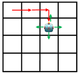
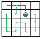
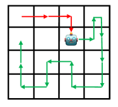
Figure 1: Consider a 4$\times$4 grid-world for illustration. (a) Agent starts at the top left corner and takes a few actions(red arrows show the trace), (b) optimal trajectory covering the grid (green arrows), (c) sub-optimal trajectory where agent visits a previously observed state in the last step, (d) another sub-optimal trajectory an observed state is visited at an earlier step.

1 Introduction

Animals and humans are very efficient at exploration compared to their data-hungry algorithms counterparts (Litman, 2005; Kidd & Hayden, 2015; Schmidhuber, 1991, 2009; Clark, 2018; Ecoffet et al., 2019; Vinyals et al., 2017; Schmidhuber, 2010). For instance, when misplacing an item, a person will methodically search through the environment to locate the lost item. To efficiently explore, an intelligent agent must consider past interactions to decide what to explore next and avoid re-visiting previously encountered locations to find rewarding states as fast as possible. Consequently, the agent needs to reason over potentially long interaction sequences, a space that grows exponentially with the sequence length. Here, assuming that all the information the agent needs to act is contained in the current state is impossible (Mutti et al., 2022a).

In this paper, we present $\eta$$\psi$-Learning, an algorithm to learn an exploration policy that methodically searches through a task. This is accomplished by maximizing the entropy of the state visitation distribution of a single finite-length trajectory. This focus on optimizing the state visitation distribution of a single trajectory distinguishes our approach from prior work on exploration methods that maximize the entropy of the state visitation distribution (Hazan et al., 2019; Tarbouriech & Lazaric, 2019; Lee et al., 2019; Mutti & Restelli, 2020; Guo et al., 2021). For example Hazan et al. (2019) focus on learning a Markovian policy—a decision-making strategy that is only conditioned on the current state and does not consider which states have been explored before. A Markovian policy constrains the agent in its ability to express different exploration policies and typically results in randomizing at uncertain states to maximize the state entropy objective. While this will lead to uniformly covering the state space in the limit, such behaviors are not favorable for real-world tasks where the agent needs to maximize state coverage with limited number of interactions.

Figure 1 presents a didactic example to illustrate how an intelligent agent can learn to efficiently explore a $4\times 4$ grid. In this example, the agent transitions between different grid cells by selecting one of four actions: up, down, left, and right. To explore optimally, the agent would select actions that maximize the entropy of the visited state distribution of the entire trajectory. Suppose the agent started its trajectory in the top left corner of the grid (shown in Figure 1) and has moved to the right twice and made one downward step (indicated by red arrows). At this point, the agent has to decide between one of the four actions to further explore the grid. For example, it could move left and follow the green trajectory as outlined in Figure 1. This path would be optimal in this example because every state is visited exactly once and not multiple times. However, the top action would lead to a sub-optimal trajectory as the agent would visit the previous state. To mitigate sub-optimal exploration, an intelligent agent must keep track of visited states to avoid revisiting states. Although taking the right action will lead to a novel state in the next step, the overall behavior will be sub-optimal as the agent will have to visit a state twice to explore the entire grid (depicted in Figures 1 and 1). This further requires an agent to carefully plan and account for the states that would follow after taking an action.

In this work, we propose $\eta$$\psi$-Learning, an algorithm to compute an exploration strategy that methodically explores within a single finite-length trajectory—as illustrated in Figure 1. $\eta$$\psi$-Learning maintains two state representations: a predecessor representation (van Hasselt et al., 2021; Bailey & Mattar, 2022) to encode past state visitation frequencies and a Successor Representation (SR) (Dayan, 1993) to predict future state visitation frequencies. The two representations are used to evaluate at every time step the decision that leads to covering all states as uniformly as possible. Specifically, for every potential action the agent can take, the SR is combined with the predecessor representation to predict the state visitation distribution for the current trajectory. Then, the action that results in the highest entropy of this state visitation distribution is selected for exploration. Furthermore, this exploration policy can be deterministic and does not randomize to achieve its maximum state entropy objective.

To summarize, the contributions of this work are as follows: Firstly, we propose a mechanism to combine successor (Dayan, 1993) and predecessor (van Hasselt et al., 2021) representations for maximizing the entropy of the state visitation distribution of a finite-length trajectory. To the best of our knowledge, this is the first work using the two representations to optimize the state visitation distribution and learn an efficient exploration policy. Secondly, we introduce $\eta$$\psi$-Learning, a method that utilizes the combination of two representations to learn deterministic and non-Markovian exploration policies for the finite-sample regime. Thirdly, we discuss how $\eta$$\psi$-Learning optimizes the entropy-based objective function for both finite and (uncountably) infinite action spaces. In Section 2 we demonstrate through empirical experiments that $\eta$$\psi$-Learning achieves optimal coverage within a single finite-length trajectory. Moreover, the visualizations presented in Section 2 demonstrate that $\eta$$\psi$-Learning learns an exploration policy that maneuvers through the state space to efficiently explore a task while minimizing the number of times the same state is revisited.

2 Related Work

The domain of exploration in Reinforcement Learning (RL) focuses on discovering an agent’s environment via intrinsic motivation to accelerate learning optimal policies. Many of the existing exploration methods seek novelty by using prediction errors  (Pathak et al., 2017; Burda et al., 2019; Sekar et al., 2020; Stadie et al., 2015) or pseudo-counts (Strehl & Littman, 2008; Bellemare et al., 2016; Machado et al., 2020). However, such methods only add an intrinsic reward signal to improve sample efficiency in a single task setting. They do not explicitly learn a policy that is designed to efficiently explore a task. In contrast, we present a method for explicitly learning an efficient exploration strategy by maximizing the entropy of a single trajectory’s state visitation distribution. We believe many subareas of RL can benefit from such efficient exploration behaviors. Some applications include Meta RL (Finn et al., 2017; Zintgraf et al., 2019; Rakelly et al., 2019; Liu et al., 2021), Continual RL (Khetarpal et al., 2020; Lehnert et al., 2017), and Unsupervised RL (Laskin et al., 2021). For example, in Meta RL an agent needs to first explore to identify which of the previously observed tasks it is in before the agent can start exploiting rewards in the current task. In this context, VariBAD (Zintgraf et al., 2019) maintains a belief over which task the agent is in given the observed interactions. While Zintgraf et al. argues that a Bayes-optimal policy implements an efficient exploration strategy, we propose a method that explicitly learns an efficient exploration policy, resulting in discovering rewarding states more efficiently than VariBAD (Section 2).

The core idea behind $\eta$$\psi$-Learning is the use of the predecessor and successor representations to predict the state visitation distribution induced by a non-Markovian policy for a single finite-length trajectory. Instead of using the successor representation for transfer, lifelong learning, or learning one representation that solve a set of tasks (Barreto et al., 2017; Zhang et al., 2017; Barreto et al., 2018; Borsa et al., 2018; Ma et al., 2018; Siriwardhana et al., 2019; Hansen et al., 2019; Barreto et al., 2020; Lehnert & Littman, 2020; Lehnert et al., 2020; Abdolshah et al., 2021; Touati & Ollivier, 2021), we use the successor representation to estimate the state visitation distribution and maximize its entropy. By using the successor representation in this way, the $\eta$$\psi$-Learning does not rely on density models (Hazan et al., 2019; Lee et al., 2019), an explicit transition model (Tarbouriech & Lazaric, 2019; Mutti & Restelli, 2020), or non-parametric estimators such as k-NN (Mutti et al., 2021). In the following sections we will discuss how $\eta$$\psi$-Learning learns a deterministic exploration policy and does not rely on randomization techniques (Mutti et al., 2021; Lee et al., 2019) or mixing multiple policies to manipulate the state visitation distribution (Lee et al., 2019; Hazan et al., 2019). Moreover, Mutti et al. (2022b) provide a theoretical analysis proving that efficient (zero regret) exploration is possible with a deterministic non-Markovian policy but computing such a policy is NP-hard. In this context, $\eta$$\psi$-Learning is to our knowledge the first algorithm for computing such an efficient exploration policy.

3 Maximum state entropy exploration

We formalize the exploration task as a Controlled Markov Process (CMP), a quadruple $\mathcal{M}=\langle\mathcal{S},\mathcal{A},p,\mu\rangle$ consisting of a (finite) state space $\mathcal{S}$, a (finite) action space $\mathcal{A}$, a transition function $p$ specifying transition probabilities with $p(s,a,s^{\prime})=\mathbb{P}(s^{\prime}|s,a)$, and a start state distribution $\mu$ specifying probability of starting a trajectory at state $s$ with $\mu(s)$. A trajectory is a sequence $\tau=(s_{1},a_{1},...,a_{h-1},s_{h})$ of some length $h$ that can be simulated in a CMP. A policy $\pi$ specifies the probabilities with which an agent selects actions when simulating a trajectory in a CMP. Typically, this policy is conditioned on the task state and specifies the probabilities of selecting a particular action in standard RL algorithms like Q-learning (Christopher, 1992; Sutton & Barto, 2018). However, as illustrated in Figure 1, the past trajectory (shown with red arrows) determines which next action leads to the best exploratory trajectory. Consequently, we consider policies that are functions of trajectories rather than just states.

The state visitation frequencies of a trajectory $\tau_{h}=(s_{1},a_{1},...,a_{h-1},s_{h})$ of length $h$ can be formally expressed in a probability vector by first encoding every state $s_{t}$ as a one-hot bit vector $\boldsymbol{e}_{s_{t}}$ and then computing the marginal across time steps for a single trajectory $\tau$:

$$\boldsymbol{\xi}_{\gamma,\tau}=\sum_{t=1}^{h}\gamma(t)\boldsymbol{e}_{s_{t}}.$$ (1)

The marginal in Equation 1 uses a discount function $\gamma:\mathbb{N}\to[0,1]$ (where we denote the set of positive integers with $\mathbb{N}$), such that $\sum_{t=1}^{h}\gamma(t)=1$. We note that this use of a discount function is distinct from using a discount factor in common RL algorithms such as Q-learning (Christopher, 1992) but using a discount function is necessary as we will elaborate in the following section.

In the example in Figure 1, the optimal exploratory agent would keep a similar visitation frequency for each state, as illustrated in Figure 1 where the optimal trajectory traverses every state once within the first 15 steps. For this trajectory the vector $\boldsymbol{\xi}_{\tau,\gamma}$ would encode a uniform probability vector, given $\gamma(t)=\frac{1}{h}$ for any $t$. In fact, an optimal exploration policy $\pi^{*}$ maximizes the entropy of marginal of this probability vector and solves the optimization problem

$$\pi^{*}\in\arg\max_{\pi}H\big{(}\mathbb{E}_{\tau}\big{[}\boldsymbol{\xi}_{\gamma,\tau}\big{]}\big{)}$$ (2)

where the expectation is computed across trajectories that are simulated in a CMP and follow the policy $\pi$. In the remainder of the paper, we will show how optimizing this objective leads to the uniform sweeping behavior illustrated in Figure 1 and the agent learns to maximize the entropy of the state visitation distribution in a single finite length trajectory. In the following section, we describe how $\eta$$\psi$-Learning optimizes the objective in Equation 2.

4 $\eta$$\psi$-Learning

To learn an efficient exploration policy, we need to estimate the state visitation history and predict the distribution over future states. Consider a trajectory $\tau=(s_{1},a_{1},...,s_{T-1},a_{T-1},s_{T},...a_{h-1},s_{h})$. At an intermediary step $T$, we denote the $T-1$-step prefix with $\tau_{:T-1}=(s_{1},a_{1},...,s_{T-1})$ and the suffix starting at step $T$ with $\tau_{T:}=(s_{T},a_{T}...,a_{h-1},s_{h})$. Using this sub-trajectory notation, the discounted state visitation distribution in Equation 1 can be written as

$$\boldsymbol{\xi}_{\gamma,\tau} =\sum_{t=1}^{T-1}\gamma(t)\boldsymbol{e}_{s_{t}}+\sum_{t=T}^{h}\gamma(t)\boldsymbol{e}_{s_{t}}.$$ (3)

Assuming the scenario presented in Section 3, suppose the agent has followed the trajectory $\tau_{:T}$ until time step $T$. At this time step, the agent needs to decide which action $a_{T}$ leads to covering the state space as uniformly as possible and maximizes the entropy of the state visitation distribution. The expected state visitation distribution for a policy $\pi$ can be expressed by conditioning on the trace $\tau_{:T}$ and a potential action $a_{T}\in\mathcal{A}$:

$$\mathbb{E}_{\tau,\pi}\Big{[}\boldsymbol{\xi}_{\gamma,\tau}\Big{|}\tau_{:T},a_{T}\Big{]}$$ (4)

$$=\mathbb{E}_{\tau,\pi}\Bigg{[}\sum_{t=1}^{T-1}\gamma(t)\boldsymbol{e}_{s_{t}}+\sum_{t=T}^{h}\gamma(t)\boldsymbol{e}_{s_{t}}\Big{|}\tau_{:T},a_{T}\Bigg{]}$$ (5)

$$=\underbrace{\sum_{t=1}^{T-1}\gamma(t)\boldsymbol{e}_{s_{t}}}_{=\boldsymbol{\eta}(\tau_{:T-1})}+\underbrace{\mathbb{E}_{\tau_{T+1:},\pi}\Bigg{[}\sum_{t=T}^{h}\gamma(t)\boldsymbol{e}_{s_{t}}\Bigg{|}\tau_{:T},a_{T}\Bigg{]}}_{=\boldsymbol{\psi}^{\pi}(\tau_{:T},a_{T})},$$ (6)

where the vector $\boldsymbol{\eta}(\tau_{:T-1})$ is a variant of the predecessor representation (van Hasselt et al., 2021; Bailey & Mattar, 2022) and the vector $\boldsymbol{\psi}^{\pi}(\tau_{:T},a_{T})$ is a variant of the successor representation (SR) (Dayan, 1993). Splitting the expected state visitation distribution into a vector $\boldsymbol{\eta}$ and $\boldsymbol{\psi}^{\pi}$ as outlined in Equation 6 is possible because we are assuming a discount function $\gamma$ as defined in Section 3. At time step $T$, the two representations can be added together to estimate the expected state visitation probability vector. Simulating the proposed algorithm is analogous to effectively drawing Monte-Carlo samples from the expectation at different steps $T$ to learn a SR and predict the expected visitation frequencies of $\boldsymbol{\xi}_{\gamma,\tau}$.

The predecessor representation vector $\boldsymbol{\eta}(\tau_{:T-1})$ can still be estimated incrementally similarly to the eligibility trace in the TD($\lambda$) algorithm (Sutton, 1988) (but with a different weighting scheme that uses the discount function $\gamma$). While the definition of the vector $\boldsymbol{\eta}(\tau_{:T})$ is similar to the definition of eligibility traces (Sutton & Barto, 2018, Chapter 12), we do not use the predecessor trace for multi-step TD updates to learn more efficiently. Instead, the vector $\boldsymbol{\eta}(\tau_{:T-1})$ estimates the visitation frequencies of past states—the predecessor states—to decide which states to explore next.

While the predecessor representation can be maintained using an update rule because the observed states are known, predicting future state visitation frequencies is more challenging. A potential solution is to exhaustively search through all possible sequences of trajectories starting from the current state. This is computationally infeasible and requires a dynamics model of the environment. Moreover, such a model is not always available, and learning them is prone to errors that compound for longer horizons (Ross et al., 2011; Janner et al., 2019). To this end, we learn a variant of the successor representation (SR), which predicts the expected frequencies of visiting future or successor states under a policy (Dayan, 1993). In contrast to previous methods which learn successor representation (SR) conditioned on the current state (Dayan, 1993; Barreto et al., 2017), $\eta$$\psi$-Learning conditions the SR on the entire history of states

$$\boldsymbol{\psi}^{\pi}(\tau_{:T},a_{T})=\mathbb{E}_{\tau_{T+1:},\pi}\left[\sum_{t=T}^{h}\gamma(t)\boldsymbol{e}_{s_{t}}\middle|\tau_{:T},a_{T}\right].$$ (7)

Conditioning the SR on the trajectory $\tau_{:T}$ is necessary because policy $\pi$ is also conditioned on $\tau_{:T}$ and therefore the visitation frequencies of future states depend on $\tau_{:T}$. Moreover, the expectation evaluates all possible trajectories after taking action $a_{T}$ at time $T$ and following policy $\pi$ afterward. We discuss in Appendix C how the SR vectors are approximated using a recurrent neural network.

We saw in Equation 6 that the predecessor representation and successor representation can be combined to predict the state visitation distribution for a policy $\pi$ and a trajectory-prefix $\tau_{:T}$. $\eta$$\psi$-Learning uses the estimated state visitation distribution to compute the entropy term in the objective defined in Equation 2. Specifically, the utility function $Q_{\text{expl}}$ approximates the entropy of the state visitation distribution for an action $a_{T}$ at every time step. By defining

$$Q_{\text{expl}}(\tau_{:T},a_{T})=H\left(\boldsymbol{\eta}(\tau_{:T-1})+\boldsymbol{\psi}^{\pi}(\tau_{:T},a_{T})\right),$$ (8)

the action that leads to the highest state visitation entropy is assigned the highest utility value. Notably, the proposed Q-function differs from prior methods using the SR, as we neither factorize the reward function (Barreto et al., 2017, 2018; Borsa et al., 2018; Touati & Ollivier, 2021) nor use the SR for learning a state abstraction (Lehnert & Littman, 2020). Optimizing the exploration Q-function stated in Equation 8 is challenging as it depends on the SR that itself depends on the policy $\pi$ which changes during learning. Furthermore, Guo et al. (2021) that the Shannon-entropy based objective is difficult to directly optimize using gradient-based methods (due to the log term inside an expectation) (Lee et al., 2019; Pong et al., 2019; Guo et al., 2021). In contrast, we outline in the following paragraphs how the entropy objective in Equation 8 can be directly optimized using either a Q-learning (Christopher, 1992) style method or a method based on the Deterministic Policy Gradient (Silver et al., 2014) framework for finite and infinite action spaces.

Finite action space framework

Since the predecessor representation is fixed for a given trajectory $\tau_{:T}$, optimizing the Q-function defined in Equation 8 boils down to predicting the optimal SR for a given history $\tau_{:T}$. Similar to prior Successor Feature learning methods (Barreto et al., 2017, 2018; Lehnert et al., 2017), we approximate the SR with a parameterized and differentiable function $\boldsymbol{\psi}_{\boldsymbol{\theta}}$ and use a loss based on a one-step temporal difference error. Given an approximation $\boldsymbol{\psi}_{\boldsymbol{\theta}}$, the SR prediction target is obtained by the current state embedding and SR of the optimal action at the next step:

$$\boldsymbol{y}(\tau_{:T+1},a^{\prime}_{T+1})=\boldsymbol{e}_{s_{T}}+\gamma(T+1)\boldsymbol{\psi_{\theta}}(\tau_{:T+1},a^{\prime}_{T+1}),$$ (9)

where $\tau_{:T+1}$ is obtained by adding action $a_{T}$ and the received next state $s_{T+1}$ to the trajectory $\tau_{:T}$. Analogous to Q-Learning (Christopher, 1992), the optimal action at the next step is specified by

$$a^{\prime}_{T+1}=\arg\max_{a\in\mathcal{A}}Q_{\text{expl}}(\tau_{:T+1},a).$$ (10)

Being greedy with respect to these entropy values to estimate the target leads to improving the policy $\pi$ which in turn finds the SR for the optimal policy. (Appendix A presents a convergence analysis of this method in a dynamic programming setting.) Then, the function $\boldsymbol{\psi}_{\boldsymbol{\theta}}$ is optimized using gradient descent on the loss function $\mathcal{L}_{SR}$, given by

$$\mathcal{L}_{SR} =||\boldsymbol{\psi}_{\boldsymbol{\theta}}(\tau_{:T},a_{T})-\boldsymbol{y}(\tau_{:T+1},a^{\prime}_{T+1})||^{2},$$ (11)

where gradients are not propagated through the target $\boldsymbol{y}(\tau_{:T+1},a^{\prime}_{T+1})$. Finally, the optimal policy selects actions greedily with respect to the $Q_{\text{expl}}$ function. Algorithm 2 describes the training procedure for the proposed variant for finite action spaces.

Infinite action space framework

Directly obtaining gradient estimates of objective defined in Equation 2 is challenging because of the expectation term in the non-linear logarithmic term. Previous approaches have used alternative optimization methods (Lee et al., 2019; Pong et al., 2019) or resorted to a simpler noise-contrastive objective function (Guo et al., 2021). In contrast with prior algorithms, we derived an $\eta$$\psi$-Learning variant for infinite action spaces that optimizes an actor-critic architecture using policy gradients to maximise the maximum state entropy objective. The agent uses an actor-critic architecture where actor and critic networks are conditioned on the history of visited states. The actor $\pi_{\mu}(\tau)$ is parameterized with a parameter vector $\mu$ and is a deterministic map from a trajectory to an action. The critic predicts the utility function conditioned on a given trajectory and action. Similar to the finite action space variant, the predecessor representation is fixed for a given trajectory and the network has to predict SR $\boldsymbol{\psi}_{\theta}(\tau,a)$ for a given trajectory $\tau$ and action $a$. Here, the target value of SR to update the critic is specified by the action obtained using the policy $a^{\prime}_{T+1}=\pi_{\mu}(\tau_{:T+1})$, given by

$$\boldsymbol{y}=\boldsymbol{e}_{s_{T}}+\gamma(T+1)\boldsymbol{\psi}_{\theta}(\tau_{:T+1},a^{\prime}_{T+1}).$$ (12)

The critic is trained with the same loss function $\mathcal{L}_{SR}$ as defined in Appendix B, where the gradients are not propagated through the target. The actor is optimized to maximize the estimated utility function (Equation 2). Since the actor is deterministic, policy gradients are computed using an adaptation of the deterministic policy gradient theorem (Silver et al., 2014). Because the actor network has no dependency on predecessor trace (which depends on the observed states only), gradients for the actor parameters are obtained by applying chain rule leading to the following gradient of Equation 8 (please refer to Proposition B.1 for more details on the derivation):

$$\nabla_{\mu}J(\pi_{\mu})=\mathbb{E}_{\tau\sim\rho}\Big{[}\sum_{i}z_{i}\nabla_{\mu}\pi_{\mu}(\tau)\nabla_{a}\boldsymbol{\psi}_{i}(\tau,a)\big{|}_{a=\pi_{\mu}(\tau)}\Big{]},$$ (13)

where $z_{i}=-\log[\boldsymbol{\eta}(\tau_{:-1})_{i}+\boldsymbol{\psi}(\tau,\pi_{\mu}(\tau))_{i}]-1$ is the multiplicative factor for state $i$, and depends on the expected probability of visiting a state. The factor $z_{i}$ can take values between between -1 and $\infty$, with positive values of high magnitude for states with low visitation probability and negative values for state with high probability of visitation. Thus, the factor $z_{i}$ scales the policy gradients to maximize the entropy of the state visitation distribution. In Algorithm 3 we outline the training procedure for the infinite action space framework.

5 Experiments

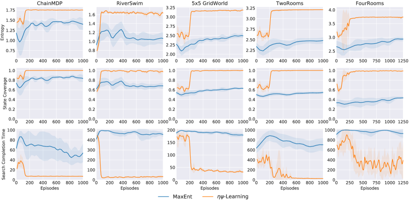
Figure 2: Comparison of $\eta$$\psi$-Learning and MaxEnt (Hazan et al., 2019) on three metrics: Entropy (top row) of state visitation distribution, State Coverage (middle row) representing the fraction of state space visited, and Search Completion Time (bottom row) denoting steps taken to cover the state space.

To analyze and test if $\eta$$\psi$-Learning learns an efficient exploration policy, we evaluate the proposed method on a set of discrete and continuous control tasks. In these experiments, we are recording a set of different performance measures to access if the resulting exploration policies do in fact maximize the entropy of the state visitation distribution and if most states are explored by $\eta$$\psi$-Learning. The following results demonstrate that by maintaining a predecessor representation and conditioning the SR on the simulated trajectory prefix, the $\eta$$\psi$-Learning agent learns a deterministic exploration policy that minimizes the number of interactions needed to visit all states. In addition, we expand our method to continuous control tasks and demonstrate how $\eta$$\psi$-Learning can efficiently explore in complex domains with infinite action space. Our method is ideal for searching out rewards in difficult sparse reward environments. We compare $\eta$$\psi$-Learning, which learns to explore an environment as efficiently as possible, to recent meta-RL methods (Zintgraf et al., 2019) that aim to learn how to optimally explore an environment to infer the rewarding or goal state.

Environments: We experiment with different tasks with both finite and infinite action spaces. The ChainMDP and RiverSwim (Strehl & Littman, 2008) is a six-state chain where the transitions are deterministic or stochastic, respectively. In these tasks a Markovian policy cannot cover the state space uniformly because the agent has to pace back and forth along the chain, visiting the same state multiple times. For the RiverSwim environment , a non-stationary policy, a policy that is a function of the time step, cannot optimally cover all states because non-determinism in the transitions can place the agent into different states at random. Furthermore, we include the $5\times 5$ grid world example used in Figure 1. We also test $\eta$$\psi$-Learning on two harder exploration tasks—the TwoRooms and FourRooms domains, which are challenging because it is not possible to obtain exact uniform visitation distribution due to the wall structure. For continuous control tasks, we evaluate on Reacher and Pusher tasks, where the agent has a robotic-arm with multiple joints. The task is to maximize the entropy over the locations covered by the fingertip of the robotic-arm. Appendix E provides more details on the environments and the hyper-parameters are reported in Appendix F.

Prior Methods: To our knowledge, existing work focusses on learning Markovian exploration policies (Mutti et al., 2022a). We use MaxEnt (Hazan et al., 2019) as a baseline agent for our experiments because this method optimizes a similar maximum entropy objective as $\eta$$\psi$-Learning—with the difference that MaxEnt learns a Markovian policy and resorts to randomization to obtain a close to uniform state visitation distribution. A comparison with SMM (Lee et al., 2019) and MEPOL (Mutti et al., 2021) is skipped because these methods optimize a similar maximum entropy objective with a Markovian policy and cannot express the same exploration behaviour as $\eta$$\psi$-Learning.

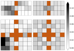
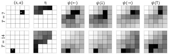
Figure 3: (a) Heatmap of state visitation distribution by unrolling a trajectory using MaxEnt (left) and $\eta$$\psi$-Learning (right) on TwoRooms and FourRooms environments. (b) Visualization of learned SR of each action (denoted with $\psi(.)$) at time steps $T=7,14$ for a trajectory using $\eta$$\psi$-Learning on $5\times 5$ grid. $(s,a)$ denotes the state (black) and action taken by the agent (direction of white arrow), $\boldsymbol{\eta}$ is the predecessor representation till time $T$ (higher values have darker shade)

.

Evaluation Metrics: Entropy measures a method’s ability to have similar visitation frequency for each state in the state space. This signifies the gap between the observed state visitation distribution and the optimal distribution that maximizes the entropy term. The Entropy metric is computed using the objective defined in Equation 2 over a single trajectory generated by the agent. A constant discount factor of $\gamma(t)=\frac{1}{h}$ is used to obtain the state visitation distribution during evaluation. An agent can maximize this measure without actually exploring all states of an environment—a desirable property for RL where rewards may be sparse and hidden in complex to-reach states. We record the state coverage metric which represents the fraction of states in the environment visited by the agent at least once within a trajectory. Lastly, we want agents to explore the state space efficiently. For example, an optimal agent can sweep through the gridworld presented in Figure 1 with a search completion time of $15$ steps ( Figure 1 shows an optimal trajectory). The search completion time metric measures the steps taken to discover each state in the environment. All results report the mean performance computed over 5 random seeds with 95% confidence intervals shading.

Quantitative Results: Figure 2 presents the results obtained for $\eta$$\psi$-Learning and MaxEnt (Hazan et al., 2019). Compared to MaxEnt, which learns a Markovian policy, $\eta$$\psi$-Learning achieves 20-50% higher entropy. This indicates that the MaxEnt algorithm by learning a Markovian and stochastic policy was randomizing at certain states which lead to sub-optimal behaviors. The performance gain was more prominent in grid-based environments because the MaxEnt agent was visiting some states more frequently than others, which are harder to explore efficiently. Furthermore, high entropy values suggest that the agent visits states with similar frequency in the environment and does not get stuck at a particular state. We attribute this behavior of $\eta$$\psi$-Learning to the proposed Q-function that picks action to visit different states and maximize the objective.

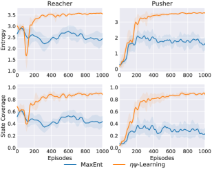
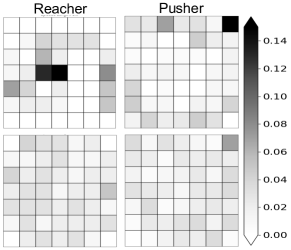
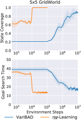
Figure 4: (a) Comparison of $\eta$$\psi$-Learning and MaxEnt (Mutti et al., 2022a) on Reacher and Pusher environments (b) Heatmaps of state visitation distribution of MaxEnt (top) and $\eta$$\psi$-Learning (bottom), (c) comparison with VariBAD (Zintgraf et al., 2019) on State Coverage and Goal Search Time metrics.

Figure 2 also shows that $\eta$$\psi$-Learning achieves optimal state coverage across environments exemplifying that $\eta$$\psi$-Learning while maximizing the entropic measure also learns to cover the state space within a single trajectory. However, the baseline MaxEnt was not able to discover all the states in the environment. MaxEnt was unable to visit all the states in ChainMDP and RiverSwim environments with trajectory length of $20$ and $50$, respectively. Moreover, the state coverage of MaxEnt was around 50-60% on the harder TwoRooms and FourRooms tasks, where the agent has to navigate between different rooms and is required to remember the order of visiting different rooms. These results reveal that Markovian policy limits an agent’s ability to maximize the state coverage in a task. The proposed method also outperformed the baseline on the search completion time metric across all environments. Notably, on ChainMDP, the $5\times 5$ gridworld, and TwoRooms environments, $\eta$$\psi$-Learning converged within 500 episodes. However, $\eta$$\psi$-Learning did not achieve optimal search exploration time on the FourRooms environment as it missed a spot in a room and resorted to it later in the episode.

To further understand the gains offered by $\eta$$\psi$-Learning, we visualized the state visitation distributions on a single trajectory (in Figure 3). On the TwoRooms environment, $\eta$$\psi$-Learning had similar density on the states in both the rooms, where the density is more around the center. This is because the agent was sweeping across rooms alternatively. $\eta$$\psi$-Learning showed a better-visited state distribution on the FourRooms environment with more distributed density across states. However, MaxEnt was not visiting all states and also visited a few states more frequently than others, elucidating the lower performance on entropy and state coverage. We further visualized the learned SR to see if $\eta$$\psi$-Learning learns a SR for the optimal exploration policy through generalized policy improvement (Barreto et al., 2017). For this analysis, we sampled a trajectory on $5\times 5$ gridworld. Figure 3 reports the heatmaps of the learned SR vector for each action at different steps in the trajectory. We observe that the SR vector for each action has lower density on the states already observed in the trace. This exemplifies that the learned SR captures the history of the visited states that further aids in taking actions to maximize the entropy of state visitation distribution. We also study if MaxEnt can show similar gains when trained with a recurrent policy (Appendix H.1) and compared the agents when evaluated across multiple trajectories (Appendix H.2).

Continuous Control tasks: The efficacy of $\eta$$\psi$-Learning is further tested on environments with infinite action space. Figure 4 reports the Entropy and State Coverage metric on Reacher and Pusher environments, where $\eta$$\psi$-Learning outperformed the baseline MaxEnt on both metrics. The gains are more significant on the Pusher environment which is a harder task because of multiple hinges in the robotic-arm. The proposed method $\eta$$\psi$-Learning achieves close to 90% coverage in both environments, whereas the MaxEnt had only close to 50% and 40% coverage on Reacher and Pusher environments, respectively. In Figure 4, heatmaps of the state visitation density for a single trajectory shows that $\eta$$\psi$-Learning has more uniformly distributed density compared to MaxEnt. The Pusher environment has high density at the top-right corner of the grid denoting the time taken by the agent to move the fingertip to other locations from the starting state. Notably, the proposed method $\eta$$\psi$-Learning has lower density at the starting state and we believe that conditioning on the history of states is guiding the agent to move the robotic-arm to other locations to maximize the entropy over the state space. In Appendix H.4, a visualization of a rolled-out trajectory generated using $\eta$$\psi$-Learning is presented showing that the agent learns to efficiently maneuver the fingertip of the robotic-arm to different locations in the environment.

Comparison with Meta-RL: A question central to Meta-RL (Finn et al., 2017; Zintgraf et al., 2019; Liu et al., 2021) is the ability to quickly explore a task and find rewarding states in complex tasks where the rewards are sparse. In this context, Zintgraf et al. (2019) present the VariBAD method, which maintains a belief over different tasks to infer the optimal policy—leading to efficient exploration behaviour that enables the agent to discover rewarding states quickly. Similar to VariBAD, the predecessor representation $\boldsymbol{\eta}$ in $\eta$$\psi$-Learning keeps track of which states have been explored and which states are not explored. Figure 4 compares the exploration behaviour of $\eta$$\psi$-Learning to VariBAD: In terms of the State Coverage and Goal Search Time metric, $\eta$$\psi$-Learning outperforms VariBAD significantly because $\eta$$\psi$-Learning is designed to optimize the entropy of the state visitation frequencies of a single trajectory instead of performing Bayes-adaptive inference across a task space. We refer the reader to Appendix G for more details.

6 Discussion

To explore efficiently, an intelligent agent needs to consider past episodic experiences to decide on the next exploratory action. We demonstrate how the predecessor representation—an encoding of past state visitations—can be combined with the successor representation—a prediction of future state visitations—to learn efficient exploration policies that maximize the state-visitation-distribution entropy. Across a set of different environments, we illustrate how $\eta$$\psi$-Learning consistently reasons across different trajectories to explore near optimally—a task that is NP-hard (Mutti et al., 2022a).

To the best of our knowledge, $\eta$$\psi$-Learning is the first algorithm that combines predecessor and successor representations to estimate the state visitation distribution. Furthermore, $\eta$$\psi$-Learning learns a non-Markovian policy and can therefore express exploration behavior not afforded by existing methods (Hazan et al., 2019; Lee et al., 2019; Mutti et al., 2021; Guo et al., 2021). To further increase the applicability of $\eta$$\psi$-Learning, one interesting direction of future research is to extend $\eta$$\psi$-Learning to POMDP environments where states are either partially observable or complex such as images. This is challenging because the agent has to learn an embedding of state observations that capture only the relevant components of the state space to maximize the entropy. We believe a promising approach would be to leverage the idea of Successor Measures (SM) (Touati & Ollivier, 2021; Touati et al., 2022; Farebrother et al., 2023) which have shown promising results when scaled to high-dimensional inputs like images. Furthermore, the presented approach can be also used for designing other algorithms that control the state visitation distribution. An application is goal-conditioned RL, where the agents need to minimize the KL divergence between visitation distribution of policy and goal-distribution (Lee et al., 2019; Pong et al., 2019). Another application is Safe RL (Wagener et al., 2021) where agents receive a penalty upon visiting unsafe states to avoid observing them.

We study reinforcement learning, which aims to enable autonomous agents to acquire search behaviors. This study of developing exploration behaviors in reinforcement learning is guided by a fundamental curiosity about the nature of autonomous learning; it has a number of potential practical applications and broad implications. First, autonomous exploration for pre-training in general, can enable autonomous agents to acquire useful skills with less human intervention and effort, potentially improving the feasibility of learning-enabled robotic systems. Second, the practical applications that we illustrate, such as applications to continuous environments, can accelerate reinforcement learning in certain settings. Specific to our method, finite length entropy maximization may also in the future offer a useful tool for search and rescue, by equipping agents with an objective that causes them to explore a space systematically to locate lost items. However, these types of reinforcement learning methods also have a number of uncertain broad implications: agents that explore the environment and attempt to acquire open-ended skills may carry out unexpected or unwanted behaviors, and would require suitable safety mechanisms of their own during training.

Appendix A Convergence Analysis

To gain a deeper understanding why the $\eta$$\psi$-Learning converges to a maximum entropy policy, we consider in this section a simplified dynamic programming variant in Algorithm 1. Note that the $\eta$$\psi$-Learning estimates the SR for a finite CMP for a finite horizon length $h$. Consequently, the trajectory-action conditioned SR $\psi^{\pi}(\tau_{:T},a)$ and exploration policy $\pi$ can be stored in an exponentially large but finite look-up table. Furthermore, with every transition an additional state is appended to the trajectory $\tau_{:T}$, meaning the agent cannot loop back to the same trajectory. Using these two properties, we state a dynamic programming variant of $\eta$$\psi$-Learning in Algorithm 1 and then prove its convergence to a policy that maximizes the entropy term $H\left(\boldsymbol{\eta}(\tau_{:T-1})+\boldsymbol{\psi}^{\pi}(\tau_{:T},a)\right)$ at every time step.

Algorithm 1 $\eta$$\psi$-Learning: Dynamic Programming Framework

1:  for all $\tau_{h},a$ do

2:     $\boldsymbol{\psi}^{\pi}(\tau_{:h},a)\leftarrow\boldsymbol{e}_{s_{h}}$

3:  end for

4:  for $t=h,...,2$ do

5:     for all $\tau_{:t},a$ do

6:        $\pi(\tau_{:t})\leftarrow\arg\max_{a}H\left(\boldsymbol{\eta}(\tau_{:t-1})+\boldsymbol{\psi}^{\pi}(\tau_{:t},a)\right)$

7:        $\boldsymbol{\psi}^{\pi}(\tau_{:t-1},a)\leftarrow\boldsymbol{e}_{s_{t-1}}+\gamma(t)\boldsymbol{\psi}^{\pi}(\tau_{:t},\pi(\tau_{:t}))$

8:     end for

9:  end for

10:  return $\pi$ such that $\pi(\tau)=\arg\max_{a}H(\boldsymbol{\eta}(\tau_{:-1})+\boldsymbol{\psi}(\tau,a))$.

The convergence proof uses the following property of the predecessor trace $\boldsymbol{\eta}$ and SR $\boldsymbol{\psi}^{\pi}$: Consider a trajectory $\tau$ which selects action $a_{T}$ at time step $T$, then

$$\boldsymbol{\eta}(\tau_{:T-1})+\boldsymbol{\psi}^{\pi}(\tau_{:T},a_{T}) =\underbrace{\sum_{t=1}^{T-1}\gamma(t)\boldsymbol{e}_{s_{t}}}_{=\boldsymbol{\eta}(\tau_{:T-1})}+\underbrace{\mathbb{E}_{\tau_{T+1:},\pi}\Bigg{[}\sum_{t=T}^{h}\gamma(t)\boldsymbol{e}_{s_{t}}\Bigg{|}\tau_{:T},a_{T}\Bigg{]}}_{=\boldsymbol{\psi}^{\pi}(\tau_{:T},a_{T})}$$ (by Eq. (6))

$$=\sum_{t=1}^{T-1}\gamma(t)\boldsymbol{e}_{s_{t}}+\mathbb{E}_{\tau_{T+1:},\pi}\Bigg{[}\gamma(T)\boldsymbol{e}_{s_{T}}+\sum_{t=T+1}^{h}\gamma(t)\boldsymbol{e}_{s_{t}}\Bigg{|}\tau_{:T},a_{T}\Bigg{]}$$ (14)

$$=\sum_{t=1}^{T}\gamma(t)\boldsymbol{e}_{s_{t}}+\mathbb{E}_{\tau_{T+1:},\pi}\Bigg{[}\sum_{t=T+1}^{h}\gamma(t)\boldsymbol{e}_{s_{t}}\Bigg{|}\tau_{:T},a_{T}\Bigg{]}$$ (15)

$$=\boldsymbol{\eta}(\tau_{:T})+\mathbb{E}_{\tau_{T+1:},\pi}\left[\boldsymbol{\psi}^{\pi}(\tau_{:T+1},\pi(\tau_{:T+1}))\middle|\tau_{:T},a_{T}\right]$$ (16)

Using this identity, we can prove the convergence of Algorithm 1.

Proposition A.1.

The policy $\pi^{*}$ returned by Algorithm 1 is such that for every $t$-step trajectory $\tau_{:t}$ where $t\leq h$,

$$\pi^{*}(\tau_{:t})\in\arg\max_{\pi}H(\boldsymbol{\eta}(\tau_{:t-1})+\boldsymbol{\psi}^{\pi}(\tau_{:t},\pi(\tau_{:t}))).$$ (17)

Proof.

The proof proceeds by induction on the length of an $h$-step trajectory, starting with a length of $h$ and iterating to a length of one.

Induction hypothesis: We define a sub-sequence optimal policy $\pi_{t}$ such that for every $k$-step trajectory prefix $\tau_{:k}$ and $t\leq k\leq h$,

$$\pi_{t}\in\arg\max_{\pi}H(\boldsymbol{\eta}(\tau_{:{k-1}})+\boldsymbol{\psi}^{\pi}(\tau_{:k},\pi(\tau_{:k}))).$$ (18)

The exploration policy $\pi_{t}$ is the optimal after executing the first $t$ steps of an $h$-step trajectory $\tau$. The goal is to prove that the induction hypothesis in line (18) holds for $t=1$.

Base case: The base case for $t=h$ holds trivially, because SR does not have a dependency on the policy $\pi$ for an $h$-step trajectory. Therefore the policy $\pi$ can output any action for a trajectory sequence of length $h$:

$$\max_{\pi}H(\boldsymbol{\eta}(\tau_{:h-1})+\boldsymbol{\psi}^{\pi}(\tau_{:h},\pi(\tau_{:h})))=H(\boldsymbol{\eta}(\tau_{:h-1})+\gamma(h)\boldsymbol{e}_{s_{h}}).$$ (19)

Induction Step: Suppose the induction hypothesis in line (18) holds for some $t>1$ and $\pi_{t}$ is the maximizer of

$$H(\boldsymbol{\eta}(\tau_{:{k-1}})+\boldsymbol{\psi}^{\pi_{t}}(\tau_{:k},\pi_{t}(\tau_{:k})))$$ (20)

where $t\leq k\leq h$. For time step $t-1$, we have that for some action $a$,

$$H(\boldsymbol{\eta}(\tau_{:t-2})+\boldsymbol{\psi}^{\pi_{t}}(\tau_{:t-1},a)) =H(\boldsymbol{\eta}(\tau_{:t-2})+\gamma(t-1)\boldsymbol{e}_{s_{t-1}}+\mathbb{E}\left[\boldsymbol{\psi}^{\pi_{t}}(\tau_{:t},\pi_{t}(\tau_{:t})\middle|s_{t-1},a\right])$$ (21)

$$=H(\boldsymbol{\eta}(\tau_{:t-1})+\mathbb{E}\left[\boldsymbol{\psi}^{\pi_{t}}(\tau_{:t},\pi_{t}(\tau_{:t}))\middle|s_{t-1},a\right])$$ (22)

$$=H(\mathbb{E}\left[\boldsymbol{\eta}(\tau_{:t-1})+\boldsymbol{\psi}^{\pi_{t}}(\tau_{:t},\pi_{t}(\tau_{:t}))\middle|s_{t-1},a\right]).$$ (23)

We note that the term inside the expectation is already maximized by $\pi_{t}$ (by induction hypothesis). If we now set $\pi_{t-1}$ to be equal to $\pi_{t}$ for every $t$-step or longer trajectory and set

$$\pi_{t-1}(\tau_{:t-1})=\arg\max_{a}H(\boldsymbol{\eta}(\tau_{:t-2})+\boldsymbol{\psi}^{\pi_{t}}(\tau_{:t-1},a)),$$ (24)

then for $t-1\leq k\leq h$

$$\pi_{t-1}\in\arg\max_{\pi}H(\boldsymbol{\eta}(\tau_{:{k-1}})+\boldsymbol{\psi}^{\pi}(\tau_{:k},\pi(\tau_{:k}))).$$ (25)

This completes the proof. ∎

Appendix B $\eta$$\psi$-Learning- Policy Gradient

Application of Q-Learning based approaches to continuous action space is not easy because finding the greedy action at any time step can be slow to be practical with large, unconstrained function approximators and nontrivial action spaces. In this work, we take a similar approach to deterministic policy gradient (Silver et al., 2014) to learn exploratory policies. The objective remains the same which is to maximize the entropy of state visitation distribution. However, it is challenging to estimate the gradient where the objective is based on the entropy term. Previous works have either used alternate optimization (Pong et al., 2019; Lee et al., 2019) or similar objective functions (Guo et al., 2021). The challenge is because of the expectation inside the logarithm in Equation 2. (Lee et al., 2019; Pong et al., 2019) addressed this intractability by first estimating the visited state distribution and then using this estimate to optimize the entropy-based objective. Unfortunately, such alternating approaches are often are prone to instability and slow convergence (Guo et al., 2021). In this work, we take an alternative direction and learn a network to directly estimate the visited state distribution. The combination of predecessor trace $\boldsymbol{\eta}$ and successor representation $\boldsymbol{\psi}^{\pi}$ can be leveraged to estimate the state visitation distribution which is obtained using:

$$\boldsymbol{\eta}(\tau_{:T-1})+\boldsymbol{\psi}^{\pi}(\tau_{:T},a_{T}) =\underbrace{\sum_{t=1}^{T-1}\gamma(t)\boldsymbol{e}_{s_{t}}}_{=\boldsymbol{\eta}(\tau_{:T-1})}+\underbrace{\mathbb{E}_{\tau_{T+1:},\pi}\Bigg{[}\sum_{t=T}^{h}\gamma(t)\boldsymbol{e}_{s_{t}}\Bigg{|}\tau_{:T},a_{T}\Bigg{]}}_{=\boldsymbol{\psi}^{\pi}(\tau_{:T},a_{T})}$$ (by Eq. (6))

The SR vector can be learned with gradient based optimization and provides the estimate of state visitation distribution for a given policy $\pi$ and trajectory. The policy can utilize this estimate to learn optimal behaviors for efficient exploration in the environment.

To learn optimal behaviors for continuous action spaces, $\eta$$\psi$-Learning uses an actor-critic architecture comprising of a deterministic actor $\pi_{\mu}(\tau)$ that provides the action and a critic to estimate the utility function. Here, both the actor and critic networks are non-Markovian and depend on the entire history of visited states. The goal of the critic network is to approximate the Q-function for a given trajectory $\tau$ and a given action $a\in\mathcal{A}$. For a given trajectory $\tau_{:T}$, critic computes this by combining the predecessor representation and the SR vector. The predecessor representation is fixed for a given history, implying that the critic only needs to approximate the SR $\boldsymbol{\psi}_{\theta}(\tau,a)$. To summarize, the critic estimates the Q-function as shown below:

$$Q_{\theta,\text{expl}}(\tau_{:T},a_{T})=H\left(\boldsymbol{\eta}(\tau_{:T-1})+\boldsymbol{\psi}_{\theta}(\tau_{:T},a_{T})\right),$$ (27)

To update the critic network, we update the SR approximator network using temporal-difference error. The target for the SR is obtained using the action coming from the current policy  $a^{\prime}_{T+1}=\pi_{\mu}(\tau_{:T+1})$, and is given by

$$\boldsymbol{y}=\boldsymbol{e}_{s_{T}}+\gamma(T+1)\boldsymbol{\psi}_{\theta}(\tau_{:T+1},a^{\prime}_{T+1}).$$ (28)

The SR network is updated with gradient-based learning to optimize the Mean-Squared Error between the predicted SR and the target, and the loss function $\mathcal{L}_{SR}$ is given by

$$\mathcal{L}_{SR} =||\boldsymbol{\psi}_{\boldsymbol{\theta}}(\tau_{:T},a_{T})-\boldsymbol{y}(\tau_{:T+1},a^{\prime}_{T+1}).||^{2}$$ (by Eq. (B))

Given an estimate of the SR for the current policy, we need a mechanism to update the actor network to maximize the objective. Deterministic policy gradient algorithm (Silver et al., 2014) provided a way of learning optimal policies with a deterministic actor. In this work, we formulate the gradient for the actor parameters using similar mechanism with the goal to maximize the entropy-based utility function. Proposition B.1 presents a derivation of the gradients for the actor network parameters obtained by applying the chain rule on the Shannon-entropy based Q-function.

Proposition B.1.

Assuming the CMP satisfies (Silver et al., 2014, conditions A.1) (all functions are continuous and differentiable across all parameters) and for a $\mu$-parameterized policy function $\pi_{\mu}$ the gradient with respect to $\mu$ of the maximum entropy objective

$$J(\pi_{\mu})=\mathbb{E}_{\tau\sim\rho}[H(\boldsymbol{\eta}(\tau_{:-1})+\boldsymbol{\psi}(\tau,\pi_{\mu}(\tau))]$$

is

$$\nabla_{\mu}J(\pi_{\mu})=\mathbb{E}_{\tau\sim\rho}\Big{[}\sum_{i}z_{i}\nabla_{\mu}\pi_{\mu}(\tau)\nabla_{a}\boldsymbol{\psi}_{i}(\tau,a)\big{|}_{a=\pi_{\mu}(\tau)}\Big{]}.$$

where $z_{i}=-\log[\boldsymbol{\eta}(\tau_{:-1})_{i}+\boldsymbol{\psi}(\tau,\pi_{\mu}(\tau))_{i}]-1$, $H$ is the Shannon-Entropy function over the representation vectors, and the expectation over trajectories is computed with respect to some trajectory visitation distribution $\rho$.

Proof.

We begin by rewriting the Shannon Entropy here for a $T$-step trajectory as

$$H(\boldsymbol{\eta}(\tau_{:T-1})+\boldsymbol{\psi}(\tau_{:T},a_{T})) =-\sum_{i}(\boldsymbol{\eta}(\tau_{:T-1})_{i}+\boldsymbol{\psi}(\tau_{:T},a_{T})_{i})\log((\boldsymbol{\eta}(\tau_{:T-1})_{i}+\boldsymbol{\psi}(\tau_{:T},a_{T})_{i}),$$ (29)

where $a_{T}=\pi_{\mu}(\tau_{:T})$.

To simplify the notations, we will use $\boldsymbol{\eta}_{i}=\boldsymbol{\eta}(\tau_{:T-1})_{i}$ and $\boldsymbol{\psi}_{i}=\boldsymbol{\psi}(\tau_{:T},a_{T})_{i}$ to represent the $i$th term of the predecessor and successor representation vectors. Now taking the gradient with respect to the actor parameters $\mu$ gives:

$$\nabla_{\mu}H(\boldsymbol{\eta}_{i}+\boldsymbol{\psi}_{i}) =-\nabla_{\mu}\sum_{i}(\boldsymbol{\eta}_{i}+\boldsymbol{\psi}_{i})\log(\boldsymbol{\eta}_{i}+\boldsymbol{\psi}_{i})$$ (30)

$$=-\sum_{i}[\nabla_{\mu}(\boldsymbol{\eta}_{i}+\boldsymbol{\psi}_{i})\log(\boldsymbol{\eta}_{i}+\boldsymbol{\psi}_{i})]$$ (31)

$$=-\sum_{i}[\log(\boldsymbol{\eta}_{i}+\boldsymbol{\psi}_{i})\nabla_{\mu}(\boldsymbol{\eta}_{i}+\boldsymbol{\psi}_{i})+(\boldsymbol{\eta}_{i}+\boldsymbol{\psi}_{i})\nabla_{\mu}\log(\boldsymbol{\eta}_{i}+\boldsymbol{\psi}_{i})]$$ (32)

$$=-\sum_{i}[\log(\boldsymbol{\eta}_{i}+\boldsymbol{\psi}_{i})\nabla_{\mu}\boldsymbol{\psi}_{i}+\nabla_{\mu}\boldsymbol{\psi}_{i}$$ (33)

$$=-\sum_{i}[\log(\boldsymbol{\eta}_{i}+\boldsymbol{\psi}_{i})+1]\nabla_{\mu}\boldsymbol{\psi}_{i}$$ (34)

Now, using the chain rule on the $i$th feature in SR, we obtain

$$\nabla_{\mu}\boldsymbol{\psi}_{i}=\nabla_{\mu}\pi_{\mu}(\tau_{:T})\nabla_{a}\boldsymbol{\psi}(\tau_{:T},a)_{i}|_{a=\pi_{\mu}(\tau_{:T})}$$ (35)

By substitution

$$\nabla_{\mu}H(\boldsymbol{\eta}_{i}+\boldsymbol{\psi}_{i})=-\sum_{i}[\log(\boldsymbol{\eta}_{i}+\boldsymbol{\psi}_{i})+1]\nabla_{\mu}\pi_{\mu}(\tau_{:T})\nabla_{a}\boldsymbol{\psi}(\tau_{:T},a)_{i}|_{a=\pi_{\mu}(\tau_{:T})}.$$ (36)

Therefore, the gradient of the overall objective is

$$\nabla_{\mu}J(\pi_{\mu}) =\mathbb{E}_{\tau\sim\rho}[\nabla_{\mu}H(\boldsymbol{\eta}(\tau_{:-1})+\boldsymbol{\psi}(\tau,\pi_{\mu}(\tau))]$$ (37)

$$=-\mathbb{E}_{\tau\sim\rho}\left[\sum_{i}[\log(\boldsymbol{\eta}_{i}+\boldsymbol{\psi}_{i})+1]\nabla_{\mu}\pi_{\mu}(\tau_{:T})\nabla_{a}\boldsymbol{\psi}(\tau_{:T},a)_{i}|_{a=\pi_{\mu}(\tau_{:T})}\right].$$ (38)

This completes the proof. ∎

In Proposition B.1, we derive the gradient of the actor parameters for the maximum state entropy exploration objective. Taking inspiration from algorithms (Lillicrap et al., 2015; Fujimoto et al., 2018; Haarnoja et al., 2018) that extend Deterministic Policy Gradient (DPG) to make the optimization process stable when scaling to larger state and action space, we base our implementation to be similar to the TD3 (Fujimoto et al., 2018) algorithm. In Appendix C, we outline the learning procedure to learn using the policy gradient derived in Proposition B.1. Furthermore, we also discuss how the proposed algorithm handles continuous state spaces.

Appendix C Neural Network Architecture

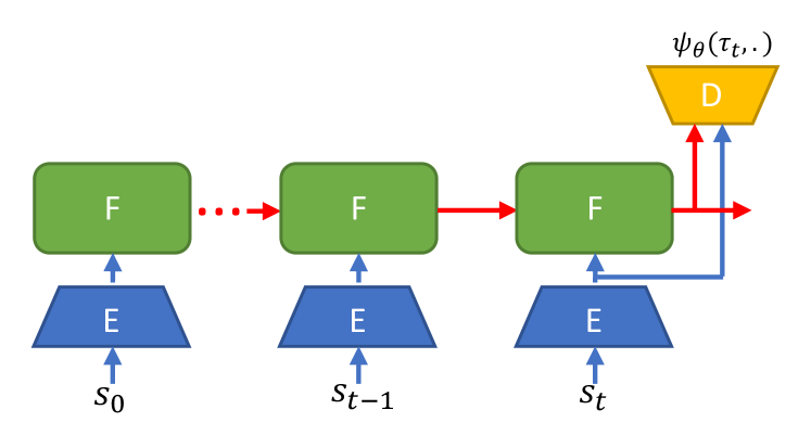
Figure 5: Network architecture to learn the SR. The states are firstly passed through an encoder (E), followed by feeding the encoded states through a RNN (GRU in our case) (F). This compresses the history of visited states, and the obtained hidden state is concatenated with the encoded state to predict the SR vector for an action using a decoder network (D).

$\eta$$\psi$-Learning approximates the SR with a parameterized function $\boldsymbol{\psi}_{\boldsymbol{\theta}}$ to learn an exploration policy and predict the state visitation distribution. Because the SR is conditioned on a trajectory $\tau$ of variable length, we implement the function $\boldsymbol{\psi}_{\boldsymbol{\theta}}$ with a Recurrent Neural Network (RNN) architecture, as outlined in Figure 5. In this architecture, the states in a trajectory $\tau_{:T}$ are first fed through a encoder network (E) comprising of Multi-Layer Perceptron (MLP) layers. Subsequently, the output of the Multi-Layer Perceptron (MLP) is fed through an Recurrent Neural Network (RNN) (denoted with F) architecture to compress the state sequence into one real-valued feature vector. Since, RNN are known to suffer from vanishing gradients (Bengio et al., 1994), we implement the RNN with a Gated Recurrent Unit (GRU) (Cho et al., 2014). Leveraging recurrent networks to learn the SR has been explored previously in (Barreto et al., 2018; Borsa et al., 2018). Finally, the recurrent state obtained from the RNN is concatenated with the representation of the current state and is passed through the the decoder (D) with MLP layers to predict an SR vector for a given action. In the following paragraphs, we elaborate on how the proposed architecture was used to train the agent for finite and infinite action spaces.

Algorithm 2 $\eta$$\psi$-Learning: Finite Action Space Framework

1:  Initialize SR network with parameters $\theta$ and the replay buffer $\mathcal{B}=\{\}$

2:  Denote the predecessor feature with $\boldsymbol{\eta}$, discount function with $\gamma$, and episode length with $h$

3:  while Training do

4:     Collect $\tau_{exp}=\{s_{1},a_{1},..,s_{h}\}$ using current policy $\pi_{\theta}$ and add it to replay buffer $\mathcal{B}$=$\mathcal{B}\cup\tau_{exp}$

5:     for each training step do

6:        Sample batch of $\tau=(s_{1},..a_{l-1},s_{l})$ $\sim$ $\mathcal{B}$ of sequence length $l\in\{2,..,h\}$

7:        Compute $a^{\prime}$= $\arg\max_{a\in\mathcal{A}}H(\boldsymbol{\eta}(\tau)+\boldsymbol{\psi}_{\theta}(\tau,a))$

8:        Compute target $\boldsymbol{y}=\boldsymbol{e}_{s_{l-1}}+\gamma(l)\boldsymbol{\psi}_{\theta}(\tau,a^{\prime})$

9:        Update SR network by performing gradient step on $||\boldsymbol{y}$ - $\boldsymbol{\psi}_{\theta}(\tau_{:l-1},a_{l-1})||_{2}^{2}$

10:     end for

11:  end while

Finite Action Space Variant

For the finite action space variant, the decoder outputs a SR vector for each action $a\in\mathcal{A}$. This is similar to prior method that learn Successor Features (SF) for discrete action spaces (Lehnert et al., 2017; Barreto et al., 2017). Algorithm 2 describes the learning procedure for training $\eta$$\psi$-Learning to get exploratory policies.

Algorithm 3 $\eta$$\psi$-Learning: Infinite Action Space Framework

1:  Initialize SR network with parameters $\theta_{1}$, $\theta_{2}$, policy parameters $\mu$ and the replay buffer $\mathcal{B}=\{\}$

2:  Set target parameters equal to the main parameters: $\theta_{targ,1}=\theta_{1}$, $\theta_{targ,2}=\theta_{2}$, and $\mu_{targ}\leftarrow\mu$

3:  Denote the predecessor feature with $\boldsymbol{\eta}$, discount function with $\gamma$, and episode length with $h$

4:  while Training do

5:     Collect $\tau_{exp}=\{s_{1},a_{1},..,s_{h}\}$ using target policy $\pi_{\mu_{targ}}$ and add it to replay buffer $\mathcal{B}$=$\mathcal{B}\cup\tau_{exp}$

6:     for each training step $j$ do

7:        Sample batch of $\tau=(s_{1},..a_{l-1},s_{l})$ $\sim$ $\mathcal{B}$ of sequence length $l\in\{2,..,h\}$

8:        Compute target actions $a^{\prime}=clip(\pi_{\mu_{targ}}(\tau_{:l})+clip(\epsilon,-c,c),a_{Low},a_{High}),\epsilon\sim\mathcal{N}(0,1)$

9:        Compute i=$\arg\min_{k\in\{1,2\}}$ $H$($\boldsymbol{\eta}(\tau_{:l-1})$ + $\boldsymbol{\psi}_{\theta_{k}}(\tau_{:l-1},a^{\prime}))$

10:        Compute target $\boldsymbol{y}$=$\boldsymbol{e}_{s_{l}}$ + $\gamma(l)$ $\boldsymbol{\psi}_{\theta_{i}}(\tau_{:l-1},a^{\prime})$

11:        Update the SR networks by performing gradient steps on                   $||\boldsymbol{y}$ - $\boldsymbol{\psi}_{\theta_{i}}(\tau_{:l-1},a_{l-1})||_{2}^{2}$,           $i=1,2$

12:        if j % policy_update == 0 then

13:           Perform update step for policy by computing gradients using                   $\sum_{i}$ $z_{i}$ $\nabla_{a}$ $\boldsymbol{\psi}_{\theta_{1}}(\tau_{:l},a)$ $|_{a=\pi(\tau_{:l})}$ $\nabla_{\mu}$ $\pi_{\mu}(\tau_{:l})$, where $z_{i}=-\log(\boldsymbol{\eta}(\tau_{:l})_{i}$ - $\boldsymbol{\psi}_{\theta_{1}}(\tau_{:l},\pi_{\mu}(\tau_{:l}))_{i})+1$

14:           Update target networks with             $\theta_{targ,i}$ $\leftarrow$ $\rho\theta_{targ,i}+(1-\rho)\theta_{i}$,           $i=1,2$             $\mu_{targ}\leftarrow\rho\mu_{targ}+(1-\rho)\mu$

15:        end if

16:     end for

17:  end while

Infinite Action Space Variant

For infinite action space variant, the hidden state from the recurrent network is passed through a deterministic actor network which comprises of MLP layers. The policy network (actor) is conditioned on the hidden states because in $\eta$$\psi$-Learning the policy is a function of trajectories and not individual states. The hidden state from the recurrent network is concatenated with the action to predict the SR vector. The estimated SR vector is used to calculate the visitation distribution over one-hot embeddings of states and these SR predictions are then used to computed to loss objective for optimization. For the Reacher and Pusher tasks, we manually sub-select which dimensions of the state space are one-hot encoded. In these cases, $\eta$$\psi$-Learning learns an exploration policy that maximizes the entropy of visitation distribution across these sub-selected dimensions only. This approach to sub-selecting state dimensions is similar to prior work on maximum state entropy exploration (Hazan et al., 2019; Mutti et al., 2022a). In this work, the agent is trained using similar techniques as the TD3 agent (Fujimoto et al., 2018). The agent keeps a single encoder and recurrent network to encode the history of observed states. The encoded states are passed through two decoder networks to predict the SR vectors, which are used to represent the two critic networks. The target for SR is computed using the vector that leads to a smaller value of the two utility functions. There is a single actor network that specifies the action from the hidden state. In addition, $\eta$$\psi$-Learning-maintains a target network for all the components—encoder, recurrent, critics, and actor networks. Furthermore, similar to the TD3 algorithm, a clipped noise is added to each dimension of the action from the target network. Moreover, we also use delayed actor updates where the actor network is updated less frequently than the SR networks. Lastly, the gradients from the actor are not passed through the encoder and the recurrent networks. The procedure for training this variant is provided in Algorithm 3.

Appendix D Discount Function

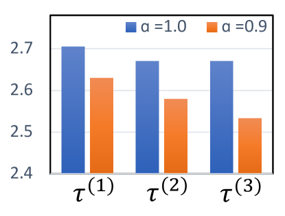
Figure 6: Illustration of the values of the entropy with different value of $\alpha$ hyperparameter in the proposed $\gamma$-function for the trajectories introduced in Figure 1.

In this work, we have used a time-dependent $\gamma$-function. Using the gridworld example described in Figure 1, we now present how the choice of $\gamma$-function affects the entropy term in the objective. Suppose there are three trajectories followed by the given trace $\tau_{:T}$, where we denote the $i$-th trajectory with $\tau^{(i)}$. Here, Figure 1 shows an optimal trajectory ($\tau^{(1)}$) which combined with the trace covers each cell of the grid with $15$ steps. Figure 1 presents a suboptimal trajectory ($\tau^{(2)}$) where the agent takes the right action from the current state and visits a previously observed state in the last step. Figure 1 shows another sub-optimal trajectory ($\tau^{(3)}$) which takes the right action in the current state but visits the new state twice because it goes to the top right corner of the grid.

For the intermediate step $T$, we define the discount factor for the predecessor representation for the trace as $\gamma(t)=\frac{\alpha^{T-t}}{Z}$, where $\alpha$ is a scalar between (0, 1], and $Z=\Sigma_{t=0}^{T}\alpha^{T-t}+\Sigma_{t=T}^{h}\alpha^{t-T}$ is the normalization factor. The $\gamma$-function for the successor representation is denoted using $\gamma(t)=\frac{\alpha^{t-T}}{Z}$. The proposed $\gamma$-function for both the representations is similar to discounting used in standard RL literature (Dayan, 1993; Sutton, 1988). Upon comparing the entropy for given trajectories with $\alpha=0.9,1.0$, we observe in  Figure 6 that $\tau^{(1)}$ being the optimal trajectory attains higher entropy when compared with $\tau^{(2)}$ and $\tau^{(3)}$. The other sub-optimal trajectories $\tau^{(2)}$ and $\tau^{(3)}$ achieve same entropy when $\alpha$ is set to 1.0. However, for $\alpha=0.9$, the discount function $\gamma$ emphasizes which states are visited earlier in the trajectory and assigns the lowest score to the trajectory $\tau^{(3)}$ because this trajectory revisits states earlier in the sequence than the other options $\tau^{(2)}$ and $\tau^{(1)}$. This example illustrates how the $\gamma$-function can be used to trade off near-term vs. long-term exploration behavior. Depending on the $\alpha$ setting, the agent can be encouraged to avoid re-visiting states either only in the short-term or the long-term, similar to how discounting encourages maximizing short-term over long-term rewards in algorithms like Q-learning (Christopher, 1992).

Appendix E Environments

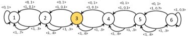
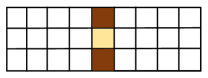
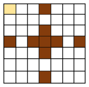
Figure 7: (a) RiverSwim (Strehl & Littman, 2008), (b) TwoRooms, and (c) FourRooms environments, respectively. The yellow block denote the initial state of the agent in each episode. The brick red regions represent the walls in the environment. When taking an action that collides with the walls, the chosen action does not change the state of the agent.

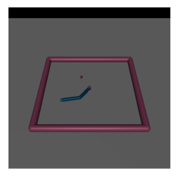
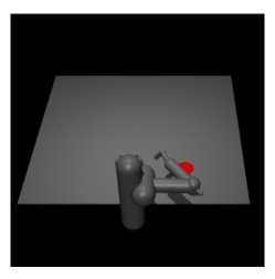
Figure 8: (a) Reacher and (b) Pusher environments for experiments with infinite action space.

For finite action space variant, we experimented with ChainMDP, RiverSwim, $5\times 5$ Grid-world, TwoRooms and FourRooms environments, which have finite action and state space, respectively. For infinite action space variant, we experiment with Reacher and Pusher environments where we want the agent to move its fingertip to different locations in the environment. The environments used in this work are further described below:

ChainMDP:

ChainMDP is an environment where the agent can take only move in two directions—left or right. In this work, we experiment with both deterministic and stochastic version of ChainMDP environments. The stochastic ChainMDP is similar to RiverSwim environment (Strehl & Littman, 2008) (Figure 7).

GridWorld:

In the Gridworld environment (shown in Figure 1), the agent can take 4 actions to move in any of the 4 directions. In this work, we experiment with the gridworld of dimensions $5\times 5$. The agent always start in the top left corner of the grid. For the gridworld, there are multiple possible optimal trajectories, and the number of such trajectories increases explonentially with size of grid.

TwoRooms:

The proposed TwoRooms environment is a gridworld with some walls. As shown in Figure 7, the agent starts at the center of wall between the two rooms and has to first navigate in one of the rooms, visit the starting state and then move to the other room. This makes the task challenging as the agents requires to track the trace because when the agents reaches initial state after exploring one room, the information of which room was visited should aid in going to the other room.

FourRooms:

The FourRooms environment (depicted in Figure 7) has four rooms connected which are connected by open shots between the walls. This task is even more challenging as the agents while navigating need to first explore the current room followed by efficiently going across different rooms.

Reacher:

The Reacher environment (shown in Figure 8) is a continuous control environment having a two-jointed robotic arm with continuous state and action spaces. The action space denotes the torques applied to the hinges. The state denotes the position, angles and angular velocities of the arms. The agent is tasked to maximize the entropy over the position of the fingertip.

Pusher:

The Pusher environment (shown in Figure 8) is a continuous control environment having a multiple-jointed robotic arm with continuous state and action spaces. The action space denotes the torques applied to the hinges. The state denotes the position, angles and angular velocities of the arms/hinges. Similar to the Reacher environment, the agent is tasked to maximize the entropy over the position of the fingertip. However, this task is harder to solve because having multiple joints leads to a larger action and state space making it a more challenging control problem.

For training and evaluation, we have used different parameters specific to each of the environment. For training, the parameters are the length of an episode and the number of episodes used for training. The number of environment steps can be obtained by multiplying these 2 parameters. For evaluation of an agent, we use different episode length for the three metrics defined to measure the performance of agents in Figure 2.

Name	ChainMDP	RiverSwim	Gridworld	TwoRooms	FourRooms
Training Parameters
Length of trajectory from environment	20	50	50	100	200
Number of episodes	1000	1000	1000	1000	2500
Evaluation Parameters
Horizon $h$ for Entropy metric	20	50	50	100	200
Horizon $h$ for State Coverage metric	20	50	50	100	200
Horizon $h$ to measure Episode Length	100	500	200	1000	1000

Table 1: Defines the parameters of the environments with discrete actions during training and evaluation, respectively.

Name	Reacher	Pusher
Training Parameters
Length of trajectory from environment	100	200
Number of episodes	1000	1000
Evaluation Parameters
Horizon $h$ for Entropy metric	100	200
Horizon $h$ for State Coverage metric	100	200

Table 2: Defines the parameters of the environments with continuous actions during training and evaluation, respectively.

Appendix F Hyper Parameters

In this section, we describe the hyperparameters used for training the proposed method $\eta$$\psi$-Learning. Table 3 and Table 4 presents the list of hyperparameters for the discrete and continuous control environments, respectively. All models were trained on a single NVIDIA V100 GPU with 32 GB memory. The implementation of the proposed method was done using the RLHive (Patil et al., 2023) library.

Name	Value
Batch Size	32
Sequence Length	10 / 20 / 50 / 50 / 100
$\alpha$ for $\gamma$-function	0.95
Encoder layers	1
Encoder output dimensions	64 / 64 / 128 / 128 / 256
Encoder activation	LeakyReLU (Yu et al., 2017)
Hidden state of GRU	64 / 64 / 128 / 128 / 256
Hidden layer dimension for SR decoder	32 / 32 / 64 / 64 / 128
Decoder activation	None
Optimizer	Adam (Kingma & Ba, 2014)
Learning rate	3e-4
Capacity of replay buffer	200000

Table 3: Hyper parameters used for training $\eta$$\psi$-Learning. When parameters are separated by /./././., it means the corresponding hyperparameters for ChainMDP, RiverSwim, Gridworld, TwoRooms and FourRooms environments, respectively. When tuning the agent for a task, we recommend searching over $\alpha\in\{0.9,0.95,0.98,0.99\}$, and hidden state dimension of GRU and encoder output dimensions in $\{64,128,256,512\}$. For the replay buffer, we have used the replay buffer implemented in DreamerV2 (Hafner et al., 2020), which for an episode samples a chunk of a given length.

Name	Value
Batch Size	256
Sequence Length	100
$\alpha$ for $\gamma$-function	0.95
Encoder layers	2
Encoder output dimensions	256
Encoder activation	LeakyReLU (Yu et al., 2017)
Hidden state of GRU	256
Hidden layer dimension for SR decoder	256
Decoder activation	None
Optimizer	Adam (Kingma & Ba, 2014)
Learning rate	3e-4
Capacity of replay buffer	200000
Polyak constant	0.005
Grad Clip	5.0
Action noise	0.1
Target noise	0.2

Table 4:  Hyper parameters used for training $\eta$$\psi$-Learning on continuous state space environments. When tuning the agent for a task, we recommend searching over $\alpha\in\{0.9,0.95,0.98,0.99\}$, and hidden state dimension of GRU and encoder output dimensions in $\{64,128,256,512\}$. For the replay buffer, we have used the replay buffer implemented in DreamerV2 (Hafner et al., 2020), which for an episode samples a chunk of a given length.

Appendix G Meta-RL

In this work, we demonstrated how $\eta\psi$-Learning can learn optimal policies that can maximize the entropy of state visitation distribution. Such policies are useful for many subareas of RL where during evaluation the task is to adapt to new reward functions with minimal interactions with the environment. A challenging subproblem in such tasks is to infer the reward function. This is especially harder when the reward is sparse. Some recent works have explored adding exploratory behaviors for initial interactions with the environment to allow agent to infer the reward function. VariBAD (Zintgraf et al., 2019) algorithm learns optimal policies that can explore during evaluation to speed up adaptation for Meta-RL tasks. VariBAD maintains a belief over the state space to explore in the environment and upon discovering the reward function adapts to the To illustrate the exploratory capabilities of $\eta$$\psi$-Learning, we compare with VariBAD as baseline in this section.

The implementation of VariBAD provided by the authors is used to conduct this experiment. The baseline was trained for 10 million environment steps on the $5\times 5$ gridworld using the setup described in the paper. Two metrics are employed to compare the agents:

• State Coverage computes the fraction of the state space covered by the agent.

• Goal Search Time computes the environment steps taken to locate the sparse reward goal state. This evaluates the ability of the agent at quickly finding the reward which is essential for swift adaptation to novel tasks.

The two metrics evaluate the agents on average time taken to find the reward function and the average search completion time for covering the grid. The VariBAD (Zintgraf et al., 2019) algorithm considered sparse reward task where a random location is sampled after each episode as the goal state and is assigned a high reward. To compute the Goal Search Time metric, we sample a goal state randomly and record the steps taken to locate the target state. For evaluation, the metric is averaged over 16 sampled goal state for each seed. Figure 4 presents the comparison of VariBAD and $\eta$$\psi$-Learning on both metrics across 5 seeds. The proposed method $\eta$$\psi$-Learning achieves outperforms VariBAD on both metrics while only being trained for 100K environment steps. This demonstrate the efficacy of $\eta$$\psi$-Learning at exploring in environment that involves inferring the reward function during evaluation. We believe $\eta$$\psi$-Learning can be combined with a adaptation policy, where the proposed method can explore to find the reward and the adaptation policy is trained to adapt quickly to the reward function, and we leave this for future work.

Appendix H Ablation Studies

In this section, we present ablations studies to understand the gains of the proposed method  $\eta$$\psi$-Learning.

H.1 MaxEnt with a recurrent network

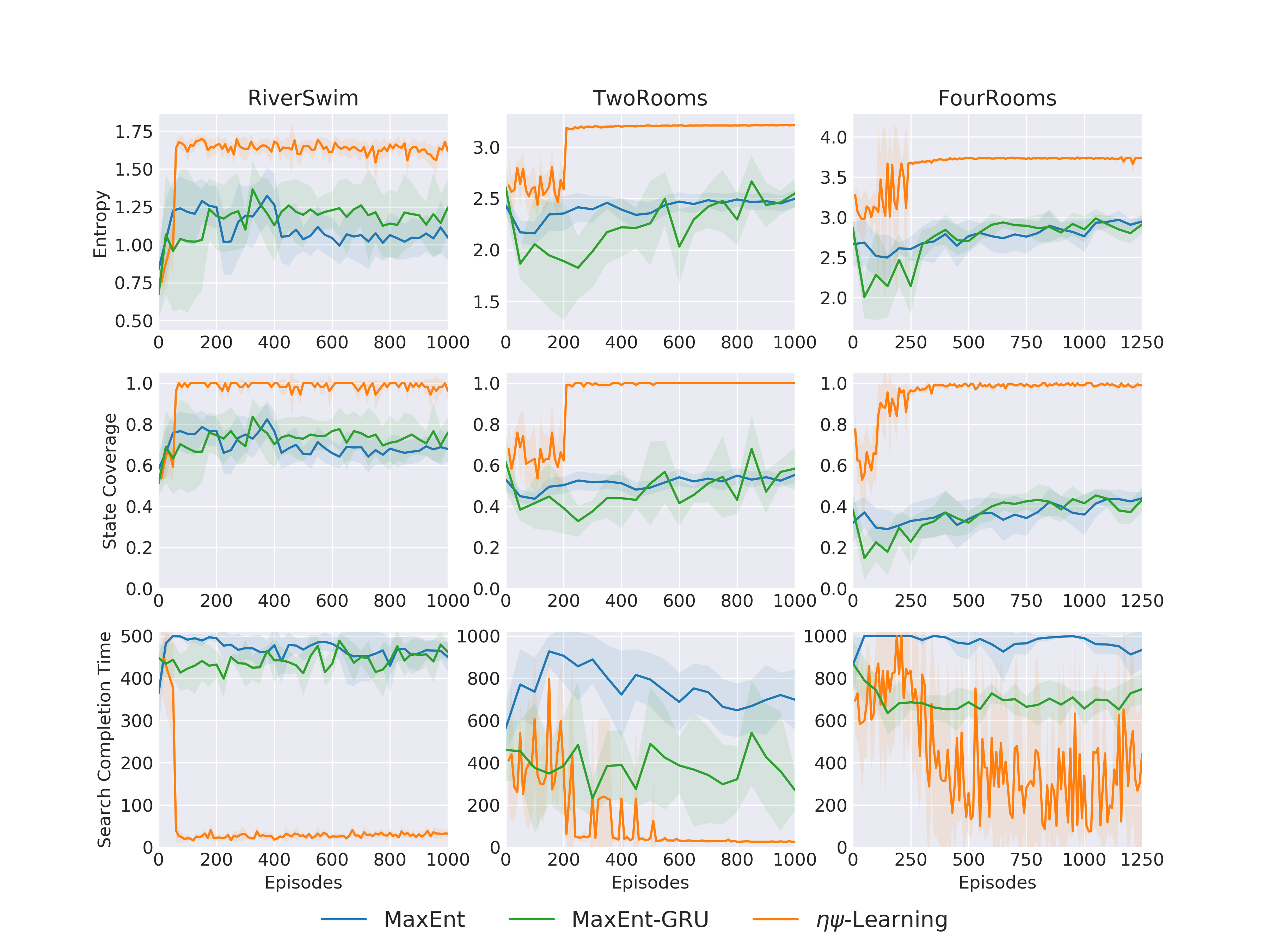
Figure 9: Comparison of the baseline MaxEnt when trained with a recurrent network.

We conduct an experiment with a modification to the baseline MaxEnt (Hazan et al., 2019) where agent observed the history of visited states. This is done to evaluate if the improvements are coming from having a recurrent policy. To this end, the state-conditioned policy in MaxEnt is replaced with a recurrent policy where the GRU (Cho et al., 2014) encodes the states observed in the trajectory. The parameters of the recurrent policy is optimized using the loss function described in MaxEnt (Hazan et al., 2019). Figure 9 presents the results of MaxEnt with a recurrent policy (named MaxEnt-GRU) where no gains are observed by having a recurrent policy and the proposed objective function used to train $\eta$$\psi$-Learning is crucial for learning optimal behaviors.

H.2 Comparison across multiple trajectories

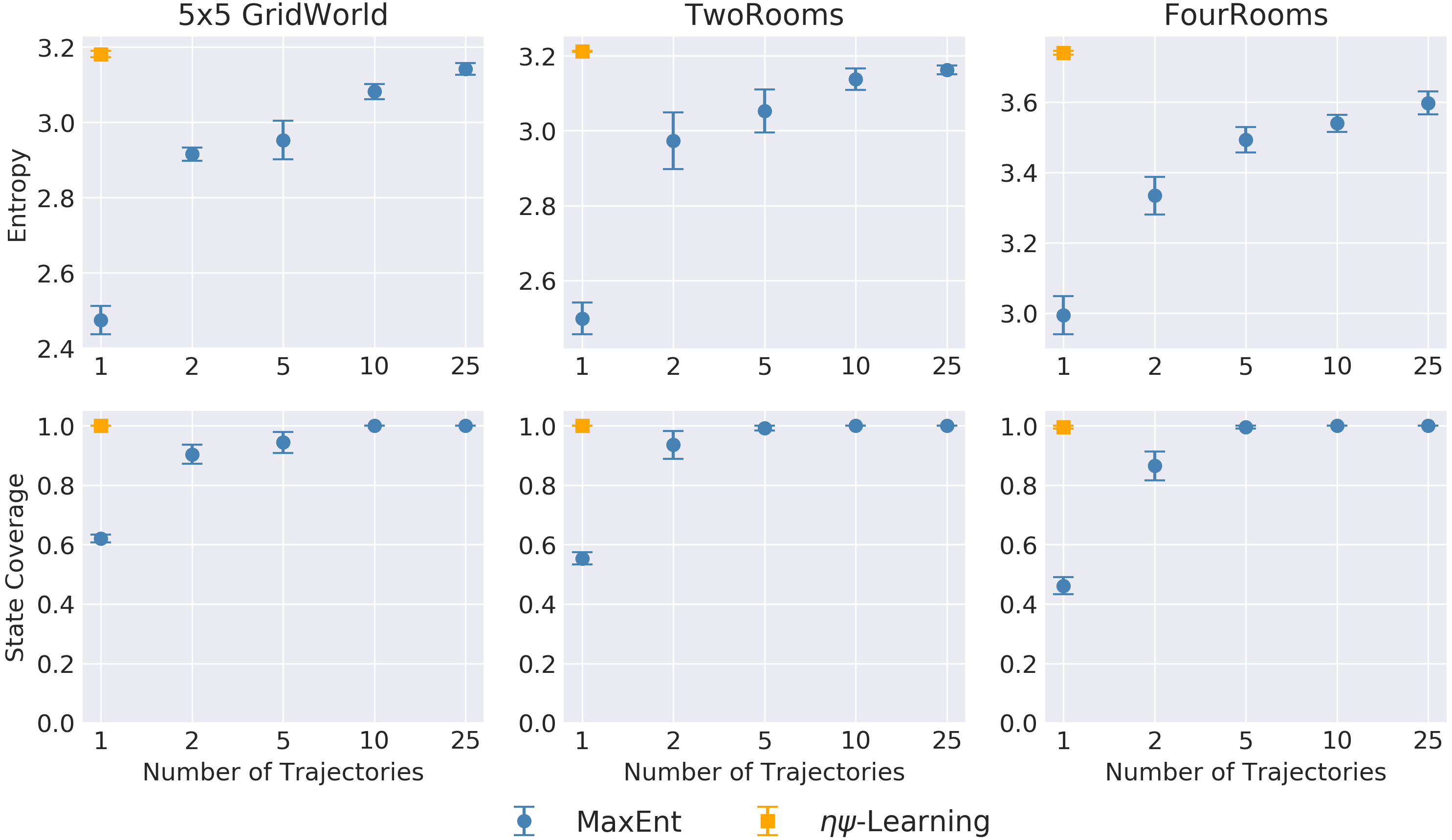
Figure 10: Comparison of $\eta$$\psi$-Learning with baseline MaxEnt when metrics are computed using multiple trajectories. MaxEnt-X denotes the evaluation with X trajectories.

Contemporary methods on Maximum State Entropy Exploration (Hazan et al., 2019; Mutti et al., 2021) were evaluated by averaging the state visitation distribution over multiple trajectories. In this work, we demonstrate that $\eta$$\psi$-Learning can achieve optimal behaviors over a single trajectory of finite length. In this study, we also explore comparison of the baseline MaxEnt when evaluated over multiple trajectories. For this evaluation, we sample a batch of trajectories and then average the state visitation distribution of trajectories. The metrics are then computed using this averaged visited state distribution. In  Figure 10, we compare the Entropy and State Coverage over this averaged distribution. MaxEnt-X denotes the metric of MaxEnt after sampling X trajectories during evaluation. The proposed method $\eta$$\psi$-Learningwas evaluated using a single trajectory. We do not report metrics of $\eta$$\psi$-Learningacross multiple trajectories as we observed that the gains do not vanish with an increasing number of trajectories. The metrics for the MaxEnt algorithm improve with the increasing number of trajectories used for evaluation. With 10 or more trajectories, the baseline achieves optimal State Coverage. However, $\eta$$\psi$-Learning achieves full coverage with a single trajectory demonstrating the efficiency of the exploration policies learned using the proposed method. The baseline MaxEnt show similar behaviors by improving on the Entropy metric with more trajectories used for evaluation, whereas $\eta$$\psi$-Learning still outperforms the baseline when evaluated using a single trajectory. This demonstrates that the proposed method explores the state-space with near-equal state visitations to maximize the entropy while having optimal state coverage in a single trajectory.

H.3 Effect of the $\alpha$ parameter

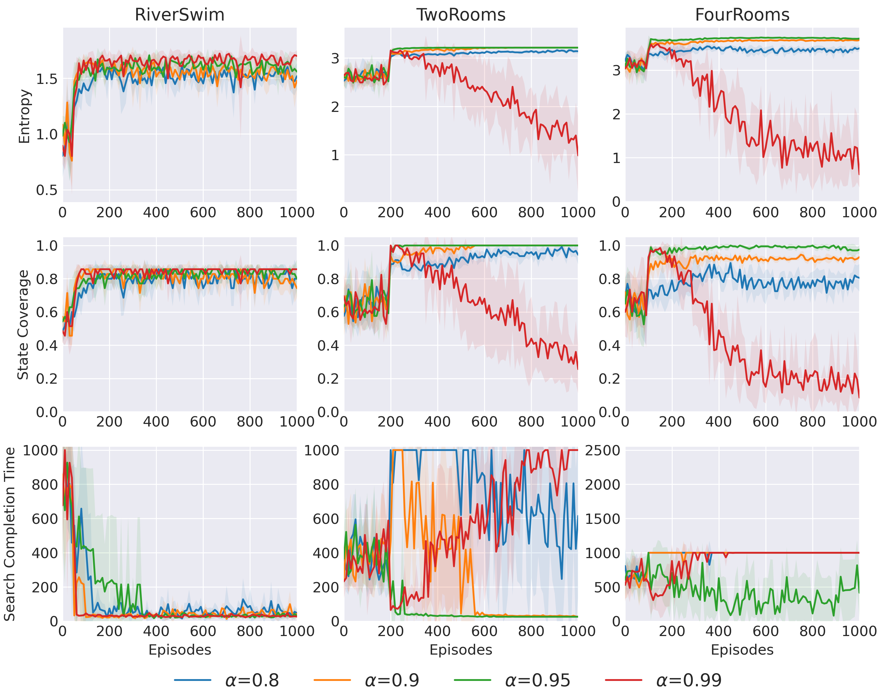
Figure 11: Evaluation with different value of $\alpha$ hyperparameter in the proposed $\gamma$-function.

We also study the effect of the hyper-parameter $\alpha$ of the $\gamma$-function (discussed in Appendix D). We note that $\alpha$ can be selected using the same method used to select the discount factor in the standard RL. We conducted experiments with $\alpha$={0.8,0.9,0.95,0.99} across three environments- RiverSwim, TwoRooms, and FourRooms (Figure 11). On the RiverSwim environment, all methods converged with similar values across all metrics. On the TwoRooms environments, agents with $\alpha$={0.8, 0.99} were not performing well across the three metrics. Moreover, the convergence was slower for agent with $\alpha=0.9$ when compared with agent trained with $\alpha=0.95$. Our intuition behind this is that when $\alpha$ is smaller, the memory of the visited states in predecessor representation ($\eta$) reduces leading to a re-visitation of observed states. Whereas when $\alpha$ is large, then the agent does similarly discount a future state at any point in the trajectory. Lastly, on the FourRooms environment, the results are similar to the TwoRooms environment but with more pronounced differences in metrics for different values of $\alpha$. This is because FourRooms environment is harder to solve than TwoRooms environments. Notably, the Search Completion Time metric diverges for all values of $\alpha\neq 0.95$, which shows that $\alpha=0.95$ leads to optimal behavior for our task. For new tasks, we believe $\alpha$ can be tuned similarly to the discount factor used in standard RL.

H.4 Visualization of trajectories

The maneuvers taken by the learned $\eta$$\psi$-Learning agent were also visualised. For the Reacher environment, the agent was first covering the faraway states followed by covering the nearby states to the central position. Similar behaviors were observed for the Pusher environment, where the agent was moving the fingertip to different locations on the table top and tried visiting all reachable locations on the table.

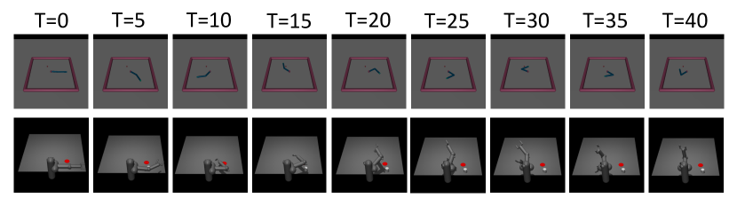
Figure 12: Rolled out trajectories using the learned $\eta$$\psi$-Learning agent on the Reacher (top row) and Pusher (bottom row) environments at different time steps, respectively.

References

- Abdolshah et al. (2021) Abdolshah, M., Le, H., George, T. K., Gupta, S., Rana, S., and Venkatesh, S. A new representation of successor features for transfer across dissimilar environments. In International Conference on Machine Learning, pp. 1–9. PMLR, 2021.
- Bailey & Mattar (2022) Bailey, D. and Mattar, M. Predecessor features. arXiv preprint arXiv:2206.00303, 2022.
- Barreto et al. (2017) Barreto, A., Dabney, W., Munos, R., Hunt, J. J., Schaul, T., van Hasselt, H. P., and Silver, D. Successor features for transfer in reinforcement learning. Advances in neural information processing systems, 30, 2017.
- Barreto et al. (2018) Barreto, A., Borsa, D., Quan, J., Schaul, T., Silver, D., Hessel, M., Mankowitz, D., Zidek, A., and Munos, R. Transfer in deep reinforcement learning using successor features and generalised policy improvement. In International Conference on Machine Learning, pp. 501–510. PMLR, 2018.
- Barreto et al. (2020) Barreto, A., Hou, S., Borsa, D., Silver, D., and Precup, D. Fast reinforcement learning with generalized policy updates. Proceedings of the National Academy of Sciences, 117(48):30079–30087, 2020.
- Bellemare et al. (2016) Bellemare, M., Srinivasan, S., Ostrovski, G., Schaul, T., Saxton, D., and Munos, R. Unifying count-based exploration and intrinsic motivation. In Advances in Neural Information Processing Systems, pp. 1471–1479, 2016.
- Bengio et al. (1994) Bengio, Y., Simard, P., and Frasconi, P. Learning long-term dependencies with gradient descent is difficult. IEEE transactions on neural networks, 5(2):157–166, 1994.
- Borsa et al. (2018) Borsa, D., Barreto, A., Quan, J., Mankowitz, D., Munos, R., Van Hasselt, H., Silver, D., and Schaul, T. Universal successor features approximators. arXiv preprint arXiv:1812.07626, 2018.
- Burda et al. (2019) Burda, Y., Edwards, H., Storkey, A., and Klimov, O. Exploration by random network distillation. In International Conference on Learning Representations, 2019. URL https://openreview.net/forum?id=H1lJJnR5Ym.
- Cho et al. (2014) Cho, K., Van Merriënboer, B., Gulcehre, C., Bahdanau, D., Bougares, F., Schwenk, H., and Bengio, Y. Learning phrase representations using rnn encoder-decoder for statistical machine translation. arXiv preprint arXiv:1406.1078, 2014.
- Christopher (1992) Christopher, J. Watkins and peter dayan. Q-Learning. Machine Learning, 8(3):279–292, 1992.
- Clark (2018) Clark, A. A nice surprise? predictive processing and the active pursuit of novelty. Phenomenology and the Cognitive Sciences, 17(3):521–534, 2018.
- Dayan (1993) Dayan, P. Improving generalization for temporal difference learning: The successor representation. Neural computation, 5(4):613–624, 1993.
- Ecoffet et al. (2019) Ecoffet, A., Huizinga, J., Lehman, J., Stanley, K. O., and Clune, J. Go-explore: a new approach for hard-exploration problems. arXiv preprint arXiv:1901.10995, 2019.
- Farebrother et al. (2023) Farebrother, J., Greaves, J., Agarwal, R., Lan, C. L., Goroshin, R., Castro, P. S., and Bellemare, M. G. Proto-value networks: Scaling representation learning with auxiliary tasks. arXiv preprint arXiv:2304.12567, 2023.
- Finn et al. (2017) Finn, C., Abbeel, P., and Levine, S. Model-agnostic meta-learning for fast adaptation of deep networks. In International conference on machine learning, pp. 1126–1135. PMLR, 2017.
- Fujimoto et al. (2018) Fujimoto, S., van Hoof, H., and Meger, D. Addressing function approximation error in actor-critic methods. arXiv preprint arXiv:1802.09477, 2018.
- Guo et al. (2021) Guo, Z. D., Azar, M. G., Saade, A., Thakoor, S., Piot, B., Pires, B. A., Valko, M., Mesnard, T., Lattimore, T., and Munos, R. Geometric entropic exploration. arXiv preprint arXiv:2101.02055, 2021.
- Haarnoja et al. (2018) Haarnoja, T., Zhou, A., Abbeel, P., and Levine, S. Soft actor-critic: Off-policy maximum entropy deep reinforcement learning with a stochastic actor. In International conference on machine learning, pp. 1861–1870. PMLR, 2018.
- Hafner et al. (2020) Hafner, D., Lillicrap, T., Norouzi, M., and Ba, J. Mastering atari with discrete world models. arXiv preprint arXiv:2010.02193, 2020.
- Hansen et al. (2019) Hansen, S., Dabney, W., Barreto, A., Van de Wiele, T., Warde-Farley, D., and Mnih, V. Fast task inference with variational intrinsic successor features. arXiv preprint arXiv:1906.05030, 2019.
- Hazan et al. (2019) Hazan, E., Kakade, S., Singh, K., and Van Soest, A. Provably efficient maximum entropy exploration. In Chaudhuri, K. and Salakhutdinov, R. (eds.), Proceedings of the 36th International Conference on Machine Learning, volume 97 of Proceedings of Machine Learning Research, pp. 2681–2691. PMLR, 09–15 Jun 2019. URL https://proceedings.mlr.press/v97/hazan19a.html.
- Janner et al. (2019) Janner, M., Fu, J., Zhang, M., and Levine, S. When to trust your model: Model-based policy optimization. Advances in Neural Information Processing Systems, 32, 2019.
- Khetarpal et al. (2020) Khetarpal, K., Riemer, M., Rish, I., and Precup, D. Towards continual reinforcement learning: A review and perspectives. arXiv preprint arXiv:2012.13490, 2020.
- Kidd & Hayden (2015) Kidd, C. and Hayden, B. Y. The psychology and neuroscience of curiosity. Neuron, 88(3):449–460, 2015.
- Kingma & Ba (2014) Kingma, D. P. and Ba, J. Adam: A method for stochastic optimization. arXiv preprint arXiv:1412.6980, 2014.
- Laskin et al. (2021) Laskin, M., Yarats, D., Liu, H., Lee, K., Zhan, A., Lu, K., Cang, C., Pinto, L., and Abbeel, P. Urlb: Unsupervised reinforcement learning benchmark. arXiv preprint arXiv:2110.15191, 2021.
- Lee et al. (2019) Lee, L., Eysenbach, B., Parisotto, E., Xing, E., Levine, S., and Salakhutdinov, R. Efficient exploration via state marginal matching. arXiv preprint arXiv:1906.05274, 2019.
- Lehnert & Littman (2020) Lehnert, L. and Littman, M. L. Successor features combine elements of model-free and model-based reinforcement learning. J. Mach. Learn. Res., 21:196–1, 2020.
- Lehnert et al. (2017) Lehnert, L., Tellex, S., and Littman, M. L. Advantages and limitations of using successor features for transfer in reinforcement learning. arXiv preprint arXiv:1708.00102, 2017.
- Lehnert et al. (2020) Lehnert, L., Littman, M. L., and Frank, M. J. Reward-predictive representations generalize across tasks in reinforcement learning. PLoS computational biology, 16(10):e1008317, 2020.
- Lillicrap et al. (2015) Lillicrap, T. P., Hunt, J. J., Pritzel, A., Heess, N., Erez, T., Tassa, Y., Silver, D., and Wierstra, D. Continuous control with deep reinforcement learning. arXiv preprint arXiv:1509.02971, 2015.
- Litman (2005) Litman, J. Curiosity and the pleasures of learning: Wanting and liking new information. Cognition & emotion, 19(6):793–814, 2005.
- Liu et al. (2021) Liu, E. Z., Raghunathan, A., Liang, P., and Finn, C. Decoupling exploration and exploitation for meta-reinforcement learning without sacrifices. In International conference on machine learning, pp. 6925–6935. PMLR, 2021.
- Ma et al. (2018) Ma, C., Wen, J., and Bengio, Y. Universal successor representations for transfer reinforcement learning. arXiv preprint arXiv:1804.03758, 2018.
- Machado et al. (2020) Machado, M. C., Bellemare, M. G., and Bowling, M. Count-based exploration with the successor representation. In Proceedings of the AAAI Conference on Artificial Intelligence, volume 34, pp. 5125–5133, 2020.
- Mutti & Restelli (2020) Mutti, M. and Restelli, M. An intrinsically-motivated approach for learning highly exploring and fast mixing policies. In Proceedings of the AAAI Conference on Artificial Intelligence, volume 34, pp. 5232–5239, 2020.
- Mutti et al. (2021) Mutti, M., Pratissoli, L., and Restelli, M. Task-agnostic exploration via policy gradient of a non-parametric state entropy estimate. In Proceedings of the AAAI Conference on Artificial Intelligence, volume 35, pp. 9028–9036, 2021.
- Mutti et al. (2022a) Mutti, M., De Santi, R., and Restelli, M. The importance of non-markovianity in maximum state entropy exploration. In Chaudhuri, K., Jegelka, S., Song, L., Szepesvari, C., Niu, G., and Sabato, S. (eds.), Proceedings of the 39th International Conference on Machine Learning, volume 162 of Proceedings of Machine Learning Research, pp. 16223–16239. PMLR, 17–23 Jul 2022a. URL https://proceedings.mlr.press/v162/mutti22a.html.
- Mutti et al. (2022b) Mutti, M., Mancassola, M., and Restelli, M. Unsupervised reinforcement learning in multiple environments. In Proceedings of the AAAI Conference on Artificial Intelligence, volume 36, pp. 7850–7858, 2022b.
- Pathak et al. (2017) Pathak, D., Agrawal, P., Efros, A. A., and Darrell, T. Curiosity-driven exploration by self-supervised prediction. In Proceedings of the IEEE Conference on Computer Vision and Pattern Recognition Workshops, pp. 16–17, 2017.
- Patil et al. (2023) Patil, D., Rahimi-Kalahroudi, A., Nekoei, H., Gottipati, S. K., Samsami, M. R., Gupta, K., Poddar, S., Zholus, A., Hashemzadeh, M., Zhao, X., and Chandar, S. Rlhive. https://github.com/chandar-lab/RLHive, 2023.
- Pong et al. (2019) Pong, V. H., Dalal, M., Lin, S., Nair, A., Bahl, S., and Levine, S. Skew-fit: State-covering self-supervised reinforcement learning. arXiv preprint arXiv:1903.03698, 2019.
- Rakelly et al. (2019) Rakelly, K., Zhou, A., Finn, C., Levine, S., and Quillen, D. Efficient off-policy meta-reinforcement learning via probabilistic context variables. In International conference on machine learning, pp. 5331–5340. PMLR, 2019.
- Ross et al. (2011) Ross, S., Gordon, G., and Bagnell, D. A reduction of imitation learning and structured prediction to no-regret online learning. In Proceedings of the fourteenth international conference on artificial intelligence and statistics, pp. 627–635. JMLR Workshop and Conference Proceedings, 2011.
- Schmidhuber (1991) Schmidhuber, J. Curious model-building control systems. In [Proceedings] 1991 IEEE International Joint Conference on Neural Networks, pp. 1458–1463. IEEE, 1991.
- Schmidhuber (2009) Schmidhuber, J. Simple algorithmic theory of subjective beauty, novelty, surprise, interestingness, attention, curiosity, creativity, art, science, music, jokes. Journal of the Society of Instrument and Control Engineers, 48(1):21–32, 2009.
- Schmidhuber (2010) Schmidhuber, J. Formal theory of creativity, fun, and intrinsic motivation (1990–2010). IEEE transactions on autonomous mental development, 2(3):230–247, 2010.
- Sekar et al. (2020) Sekar, R., Rybkin, O., Daniilidis, K., Abbeel, P., Hafner, D., and Pathak, D. Planning to explore via self-supervised world models. In ICML, 2020.
- Silver et al. (2014) Silver, D., Lever, G., Heess, N., Degris, T., Wierstra, D., and Riedmiller, M. Deterministic policy gradient algorithms. In International conference on machine learning, pp. 387–395. Pmlr, 2014.
- Siriwardhana et al. (2019) Siriwardhana, S., Weerasakera, R., Matthies, D. J., and Nanayakkara, S. Vusfa: Variational universal successor features approximator, 2019.
- Stadie et al. (2015) Stadie, B. C., Levine, S., and Abbeel, P. Incentivizing exploration in reinforcement learning with deep predictive models. arXiv preprint arXiv:1507.00814, 2015.
- Strehl & Littman (2008) Strehl, A. L. and Littman, M. L. An analysis of model-based interval estimation for markov decision processes. Journal of Computer and System Sciences, 74(8):1309–1331, 2008.
- Sutton (1988) Sutton, R. S. Learning to predict by the methods of temporal differences. Machine learning, 3(1):9–44, 1988.
- Sutton & Barto (2018) Sutton, R. S. and Barto, A. G. Reinforcement learning: An introduction. MIT press, 2018.
- Tarbouriech & Lazaric (2019) Tarbouriech, J. and Lazaric, A. Active exploration in markov decision processes. In The 22nd International Conference on Artificial Intelligence and Statistics, pp. 974–982. PMLR, 2019.
- Touati & Ollivier (2021) Touati, A. and Ollivier, Y. Learning one representation to optimize all rewards. Advances in Neural Information Processing Systems, 34:13–23, 2021.
- Touati et al. (2022) Touati, A., Rapin, J., and Ollivier, Y. Does zero-shot reinforcement learning exist? arXiv preprint arXiv:2209.14935, 2022.
- van Hasselt et al. (2021) van Hasselt, H., Madjiheurem, S., Hessel, M., Silver, D., Barreto, A., and Borsa, D. Expected eligibility traces. In Proceedings of the AAAI Conference on Artificial Intelligence, volume 35, pp. 9997–10005, 2021.
- Vinyals et al. (2017) Vinyals, O., Ewalds, T., Bartunov, S., Georgiev, P., Vezhnevets, A. S., Yeo, M., Makhzani, A., Küttler, H., Agapiou, J., Schrittwieser, J., et al. Starcraft ii: A new challenge for reinforcement learning. arXiv preprint arXiv:1708.04782, 2017.
- Wagener et al. (2021) Wagener, N. C., Boots, B., and Cheng, C.-A. Safe reinforcement learning using advantage-based intervention. In International Conference on Machine Learning, pp. 10630–10640. PMLR, 2021.
- Yu et al. (2017) Yu, Y., Gong, Z., Zhong, P., and Shan, J. Unsupervised representation learning with deep convolutional neural network for remote sensing images. In International conference on image and graphics, pp. 97–108. Springer, 2017.
- Zhang et al. (2017) Zhang, J., Springenberg, J. T., Boedecker, J., and Burgard, W. Deep reinforcement learning with successor features for navigation across similar environments. In 2017 IEEE/RSJ International Conference on Intelligent Robots and Systems (IROS), pp. 2371–2378. IEEE, 2017.
- Zintgraf et al. (2019) Zintgraf, L., Shiarlis, K., Igl, M., Schulze, S., Gal, Y., Hofmann, K., and Whiteson, S. Varibad: A very good method for bayes-adaptive deep rl via meta-learning. arXiv preprint arXiv:1910.08348, 2019.