Stability of optimal shapes and convergence of thresholding algorithms in linear and spectral optimal control problems

Abstract

We prove the convergence of the fixed-point (also called thresholding) algorithm in three optimal control problems under large volume constraints. This algorithm was introduced by Céa, Gioan and Michel, and is of constant use in the simulation of $L^{\infty}-L^{1}$ optimal control problems. In this paper we consider the optimisation of the Dirichlet energy, of Dirichlet eigenvalues and of certain non-energetic problems. Our proofs rely on new diagonalisation procedure for shape hessians in optimal control problems, which leads to local stability estimates.

Keywords: Convergence analysis, Numerical algorithms in optimal control, PDE constrained optimisation, Shape optimisation, Quantitative inequalities, Thresholding scheme.

AMS classification (2020): 49M05, 49M41, 49N05, 49Q10.

1 Introduction

1.1 Scope of the paper: the fixed point algorithm of Céa, Gioan and Michel for optimal control problems

The fixed-point algorithm, also dubbed thresholding algorithm, is ubiquitous in the numerical simulations of optimal control problems [6, 7, 10, 24, 27, 28, 29, 30, 43, 46]. It was first introduced by Céa, Gioan & Michel in the seminal [8]. This algorithm is designed to solve optimal control problems subject to constraints expressed in $L^{1}$ and $L^{\infty}$ norms. These problems are part of a broad class of optimal control problems writing:

$$\max_{f\in\mathcal{F}}\left(J(f):=\int_{\Omega}j(u_{f},{\nabla}u_{f})\right)\text{ where }\begin{cases}-\nabla\cdot(A{\nabla}u_{f})=F(x,u_{f})+H(f,u_{f})\,,\\ \mathcal{B}u_{f}=0\end{cases} \mathbb{P}$$ ()

where $\mathcal{B}$ is a boundary conditions operator, $A$ is an elliptic matrix and $H$ accounts for the coupling between the state $u_{f}$ and the control $f$. The admissible class of controls is of the form

$$\mathcal{F}:=\left\{f\in L^{\infty}({\Omega}):\quad 0\leqslant f\leqslant 1\text{ a.e., }\fint_{\Omega}f=V_{0}\right\}$$

for some volume constraint $V_{0}\in(0;1)$. In most cases, no explicit description of the maximisers is available and the algorithm proposed in [8] can be recast in terms of the so-called switch function: provided all functionals at hand are regular enough we may represent, for a given $f\in\mathcal{F}$, the derivative of the criterion through a function $p_{f}$, called the switch function of the optimal control problem: for any admissible perturbation $h$ at $f$ (for the sake of simplicity, such that for any ${\varepsilon}>0$ small enough $f+{\varepsilon}h\in\mathcal{F}$; see Definition 3 for the proper notion), the derivative of $J$ at $f$ in the direction $h$ writes

$$\dot{J}(f)[h]=\int_{\Omega}hp_{f}.$$

The thresholding algorithm, in short, picks the direction $h$ that maximises $\dot{J}(f)[\cdot]$:

Algorithm 1 Thresholding algorithm

1:Initialisation at $f_{0}\in\mathcal{F}$

2:$k\leftarrow 0$

3:Compute $p_{f_{k}}$

4:Compute $c_{k}$ such that $\mathrm{Vol}(\{p_{f_{k}}>c_{k}\})=V_{0}\mathrm{Vol}({\Omega})$.

5:$f_{k}\leftarrow\mathds{1}_{\{p_{f_{k}}>c_{k}\}}$

6:$k\leftarrow k+1$.

Some difficulties can arise. Indeed, we can only hope for this algorithm to be well-posed if the solutions to the optimal control problem ($\mathbb{P}$) only has so-called bang-bang solutions i.e. any optimal $f^{*}$ writes $f^{*}=\mathds{1}_{E^{*}}$ for some measurable $E^{*}$. Indeed, in general, one can only define a Lagrange multiplier $c_{k}$ such that

$$\mathrm{Vol}(\{p_{f_{k}}>c_{k}\})\leqslant V_{0}\mathrm{Vol}({\Omega})<\mathrm{Vol}(\{p_{f_{k}}\geqslant c_{k}\}).$$

For the algorithm to be properly defined, one needs to ensure that the level-set $\{p_{f_{k}}=c_{k}\}$ has zero measure, which “usually” implies that ($\mathbb{P}$) indeed satisfies this bang-bang property. Observe that some simple linear control problems do not satisfy this property [42]. But even assuming this is not a problem, and despite the fact that this method has proved very efficient in past contributions, the theoretical convergence of the sequence of iterates was, to the best of our knowledge, never proved apart from cases where explicit computations are available; see [29] where a detailed study of the convergence rate of the method in the one-dimensional case is undertaken. In [8, Condition (2.4)] a sufficient condition for the convergence of the algorithm is given for very specific types of functionals; some of the conditions given in this paper that ensure convergence are similar and are akin to a coercivity condition in shape differentiation [16]. Finally, we mention that in [18] a study of convergence rate for discretised version of shape optimisation algorithms is obtained.

The purpose of this paper is to study Algorithm 1 for three optimal control problems and to establish its global convergence for large volume constraints $V_{0}$. This is done by building on recent progress in the study of quantitative inequalities in optimal control theory [37, 39], and by introducing a new diagonalisation procedure for shape hessians in optimal control theory. Such a procedure is of independent interest and relates to stability estimates in optimal control theory.

Plan of the article

In section 1.2 we lay out our notations and introduce our admissible classes. We study three different problems; the introduction is divided accordingly.

• First, we consider the optimisation of the Dirichlet energy, that is, the optimisation problem

  $$\min_{f\in\mathcal{F}}\frac{1}{2}\int_{\Omega}|{\nabla}u_{f}|^{2}-\int_{\Omega}fu_{f}\text{ subject to }\begin{cases}-\Delta u_{f}=f&\text{ in }{\Omega}\,,\\ u_{f}=0&\text{ on }\partial{\Omega}.\end{cases}$$

  We refer to section 1.3 of this introduction.

• Second, we consider the optimisation of weighted Dirichlet eigenvalues, that is, the optimisation problem

  $$\min_{f\in\mathcal{F}}\lambda(f)\text{ where $\lambda(f)$ is the first Dirichlet eigenvalue of $-\Delta-f$}$$

  We underline that this is a bilinear control problem. We refer to Section 1.4.

• Third, we consider a non-energetic optimal control problem: for a given function $j=j(x,u)$ that is convex in $u$ we seek to solve

  $$\max_{f\in\mathcal{F}}J(f):=\int_{\Omega}j(x,u_{f})\text{ subject to }\begin{cases}-\Delta u_{f}=f&\text{ in }{\Omega}\,,\\ u_{f}=0&\text{ on }\partial{\Omega}.\end{cases}$$

  We refer to section 1.5.

For the sake of readability, we give in section 1.6 the general plan of the proof of convergence. The core of the paper is devoted to the proofs of the result for the Dirichlet energy. As the proofs for the other two problems are very similar we postpone them to appendices. In the conclusion of this article, we discuss several limits of our analysis and offer possible future research directions.

Related algorithms.

Before we move on to the main part of the introduction, let us mention that Algorithm 1 is linked to the thresholding algorithm, studied in detail since its introduction in [40] and which, broadly speaking, seeks to approximate mean-curvature motions using a thresholding of the solutions to certain PDEs. The theoretical and numerical aspects of this scheme have been the subject of an intense research activity in the past years [4, 19, 25, 26, 31, 32, 44, 45]. Let us mention that most of the methods used in the aforementioned works can not be used here as they use the behaviour of solutions of PDEs defined in $\textnormal{I\kern-2.10007ptR}^{d}$. The presence of boundary conditions in the models under consideration here prohibits relying on the tools these authors developed .

Finally, it should be mentioned that a closely related fixed-point type algorithm was used in [3, 2] to numerically solve topological optimization problems.

1.2 Notational conventions, preliminary definitions and setting

Throughout the paper, ${\Omega}$ is a fixed $\mathscr{C}^{2}$ bounded domain of $\textnormal{I\kern-2.10007ptR}^{d}$ ($d\geqslant 2$) which is simply connected (in particular $\partial{\Omega}$ is a connected smooth submanifold of $\textnormal{I\kern-2.10007ptR}^{d}$). For a fixed volume constraint $V_{0}\in(0;1)$ we define the set of admissible controls

$$\mathcal{F}(V_{0}):=\left\{f\in L^{\infty}({\Omega}):\,0\leqslant f\leqslant 1\text{ a.e., }\fint_{\Omega}f=V_{0}\right\}. \mathbb{Adm}$$ ()

By [22, Proposition 7.2.17] the set $\mathcal{F}(V_{0})$ is convex and closed for the weak $L^{\infty}-*$ topology. Moreover, its extreme points are characteristic functions of subsets: using $\mathrm{Extr}(X)$ to denote the extreme points of a convex set $X$ we have

$$\mathrm{Extr}(\mathcal{F}(V_{0}))=\left\{\mathds{1}_{E}\,,E\subset{\Omega}\,,\mathrm{Vol}(E)=V_{0}\mathrm{Vol}({\Omega})\right\}.$$

It is convenient to introduce a bit of terminology:

Definition 1.

A bang-bang function of $\mathcal{F}(V_{0})$ is an extreme point of $\mathcal{F}(V_{0})$.

In other words, $m$ is bang-bang in $\mathcal{F}(V_{0})$ if, and only if, there exists a measurable subset $E\subset{\Omega}$ such that $\mathrm{Vol}(E)=V_{0}\mathrm{Vol}({\Omega})$ and such that $m=\mathds{1}_{E}$.

Remark 2.

A salient feature of all the optimisation problems we consider in this paper is that their solutions are bang-bang functions. We explain in the conclusion why we can not at this point bypass this underlying assumption.

Finally, as our proofs rely on optimality conditions, we need to introduce the tangent cone to an element $f\in\mathcal{F}(V_{0})$.

Definition 3.

Let $f\in\mathcal{F}(V_{0})$. The tangent cone to $\mathcal{F}(V_{0})$ at $f$ is the set of functions $h\in L^{\infty}({\Omega})$ such that, for any sequence $\{t_{k}\}_{k\in\textnormal{I\kern-1.47005ptN}}$ converging to 0, there exists a sequence $\{h_{k}\}_{k\in\textnormal{I\kern-1.47005ptN}}$ that converges strongly to $h$ in $L^{2}({\Omega})$ and such that, for any $k\in\textnormal{I\kern-2.10007ptN}$, $f+t_{k}h_{k}\in\mathcal{F}(V_{0})$. Functions belonging to this tangent cone are called admissible perturbations at $f$.

Further characterisations of the tangent cone are available in [5, 15].

1.3 Optimisation of the Dirichlet energy

The energy functional and the optimal control problem.

The first problem we study is the optimisation of the Dirichlet energy. For a given $f\in L^{2}({\Omega})$, let $u_{f}\in W^{1,2}_{0}({\Omega})$ be the unique solution of

$$\begin{cases}-\Delta u_{f}=f&\text{ in }{\Omega}\,,\\ u_{f}=0&\text{ on }\partial{\Omega}.\end{cases}$$ (1.1)

This equation has a variational formulation: $u_{f}$ is the unique minimiser in $W^{1,2}_{0}({\Omega})$ of the energy $\mathcal{E}_{f}$ defined as

$$\mathcal{E}_{f}:W^{1,2}_{0}({\Omega})\ni u\mapsto\frac{1}{2}\int_{\Omega}|{\nabla}u|^{2}-\int_{\Omega}fu.$$

The Dirichlet energy associated with $f$ is defined by

$$\mathscr{E}(f):=\mathcal{E}_{f}(u_{f})=\frac{1}{2}\int_{\Omega}|{\nabla}u_{f}|^{2}-\int_{\Omega}fu_{f}.$$ (1.2)

The optimal control problem is

$$\framebox{$\displaystyle\min_{f\in\mathcal{F}(V_{0})}\mathscr{E}(f).$} \mathbb{P}_{\mathrm{Dir}}$$ ()

The following result is standard.

Lemma 4.

The problem ($\mathbb{P}_{\mathrm{Dir}}$) has a solution. Furthermore, the map $\mathscr{E}$ is strictly concave. In particular any solution $f^{*}$ of ($\mathbb{P}_{\mathrm{Dir}}$) is a bang-bang function in the sense of Definition 1: there exists $E^{*}\subset{\Omega}$ such that $f^{*}=\mathds{1}_{E^{*}}$, with $\mathrm{Vol}(E^{*})=V_{0}\mathrm{Vol}({\Omega}).$

The switch function and the thresholding algorithm.

To describe the thresholding algorithm we need to specify the switch function of $\mathscr{E}$. The following lemma is well-known.

Lemma 5.

The map $f\mapsto\mathscr{E}(f)$ is Fréchet differentiable at any $f\in\mathcal{F}(V_{0})$ and, for any $f\in\mathcal{F}(V_{0})$, for any admissible perturbation $h$, there holds

$$\dot{\mathscr{E}}(f)[h]=-\int_{\Omega}hu_{f}.$$

Consequently, for the Dirichlet energy, the switch function of the optimal control problem is $-u_{f}$. This allows to describe the thresholding algorithm:

Algorithm 2 Thresholding algorithm for the Dirichlet energy

1:Initialisation at $f_{0}\in\mathcal{F}$

2:$k\leftarrow 0$

3:Compute $u_{f_{k}}$

4:Compute $c_{k}$ such that $\mathrm{Vol}(\{u_{f_{k}}>c_{k}\})=V_{0}\mathrm{Vol}({\Omega})$.

5:$f_{k}\leftarrow\mathds{1}_{\{u_{f_{k}}>c_{k}\}}$

6:$k\leftarrow k+1$.

Remark 6.

Of course we have the same problem as in Algorithm 1, namely, that we would need to ensure that the algorithm is well-defined in the sense that for any index $k$ there indeed exists a $c_{k}\in\textnormal{I\kern-2.10007ptR}$ such that $\mathrm{Vol}(\{u_{f_{k}}>c_{k}\})=V_{0}\mathrm{Vol}({\Omega})$. This is also covered by our theorem.

Some terminology.

We introduce the following definition:

Definition 7 (Critical points).

For any $V_{0}\in(0;1)$, for any $f\in\mathcal{F}(V_{0})$, we say $f$ is a critical point of $\mathscr{E}$ if:

1. There exists a unique $\mu_{f}=\mu_{u_{f},V_{0}}$ such that

   $$\mathrm{Vol}(\{u_{f}>\mu_{f}\})=V_{0}\mathrm{Vol}({\Omega})=\mathrm{Vol}(\{u_{f}\geqslant\mu_{f}\}),$$

2. $f=\mathds{1}_{\{u_{f}>\mu_{f}\}}.$

A critical set is a subset $E$ of ${\Omega}$ such that $\mathds{1}_{E}\in\mathcal{F}(V_{0})$ and such that $\mathds{1}_{E}$ is a critical point of $\mathscr{E}$.

It is natural to expect that the algorithm will converge to a local minimiser of the functional. In general, one must clarify the meaning behind “local minimiser”; more than mere local minimisers we use the notion of “stable local minimisers”. Our definition here is the following:

Definition 8.

An admissible control $f^{*}\in\mathcal{F}(V_{0})$ is called a stable local minimiser of $\mathscr{E}$ in $\mathcal{F}(V_{0})$ if there exist $C=C(f^{*})\,,\delta=\delta(f^{*})>0$ such that

$$\forall f\in\mathcal{F}(V_{0})\,,\|f-f^{*}\|_{L^{1}({\Omega})}\leqslant\delta(f^{*})\Rightarrow\mathscr{E}(f)\geqslant\mathscr{E}(f^{*})+C(f^{*})\|f-f^{*}\|_{L^{1}({\Omega})}^{2}.$$

Main result

Our main result is the following:

Theorem I.

There exists ${\varepsilon}>0$ such that, if $1-{\varepsilon}\leqslant V_{0}<1$, for any initialisation $f_{0}\in\mathcal{F}(V_{0})$, the sequence $\{f_{k}\}_{k\in\textnormal{I\kern-1.47005ptN}}$ generated by Algorithm 2 converges strongly in $L^{1}({\Omega})$ to a stable local minimiser of $\mathscr{E}$ in $\mathcal{F}(V_{0})$.

1.4 Optimisation of weighted eigenvalues

The energy functional and the optimal control problem.

The second functional under consideration is the principal eigenvalue of a Dirichlet operator. For any $f\in\mathcal{F}(V_{0})$, let $\lambda(f)$ be the first eigenvalue of the operator $-\Delta-f$ endowed with Dirichlet boundary conditions. The variational formulation of $\lambda(f)$ is

$$\lambda(f)=\min_{u\in W^{1,2}_{0}({\Omega})\backslash\{0\}}\frac{\int_{\Omega}|{\nabla}u|^{2}-\int_{\Omega}fu^{2}}{\int_{\Omega}u^{2}}.$$ (1.3)

It is standard to see that this eigenvalue is simple and that any associated eigenfunction has constant sign. Thus, up to normalisation, the eigenpair $(\eta_{f},\lambda(f))$ satisfies

$$\begin{cases}-\Delta\eta_{f}=\lambda(f)\eta_{f}+f\eta_{f}&\text{ in }{\Omega}\,,\\ \eta_{f}\in W^{1,2}_{0}({\Omega})\,,\\ \eta_{f}>0&\text{ in }{\Omega}\,,\\ \int_{\Omega}\eta_{f}^{2}=1.\end{cases}$$ (1.4)

The optimal control problem under consideration is

$$\framebox{$\displaystyle\min_{f\in\mathcal{F}(V_{0})}\lambda(f).$} \mathbb{P}_{\mathrm{Eigen}}$$ ()

This problem has been studied at length, see [21, Chapter 8] or the more recent [30]. Part of the recent interest in it is due to its applications in spatial ecology, as the sign of $\lambda(f)$ predicts extinction or survival of a species, see [36, Introduction] and the references therein. The thresholding algorithm was applied to this problem in [24, 27, 30].

Similar to Lemma 4, we have the following result.

Lemma 9.

The problem ($\mathbb{P}_{\mathrm{Eigen}}$) has a solution. Furthermore, the map $\lambda$ is strictly concave. In particular any solution $f^{*}$ of ($\mathbb{P}_{\mathrm{Eigen}}$) is a bang-bang function in the sense of Definition 1: there exists $E^{*}\subset{\Omega}$ such that $f^{*}=\mathds{1}_{E^{*}}$, with $\mathrm{Vol}(E^{*})=V_{0}\mathrm{Vol}({\Omega}).$

The switch function and the thresholding algorithm.

Let us now give the switch function of ($\mathbb{P}_{\mathrm{Eigen}}$).

Lemma 10.

The map $f\mapsto\lambda(f)$ is Fréchet differentiable at any $f\in\mathcal{F}(V_{0})$ and, for any $f\in\mathcal{F}(V_{0})$, for any admissible perturbation $h$ at $f$, there holds

$$\dot{\lambda}(f)[h]=-\int_{\Omega}h\eta_{f}^{2}.$$

Consequently, for the Dirichlet eigenvalue, the switch function is $-\eta_{f}^{2}$. Note that as $\eta_{f}>0$, computing a level-set of $\eta_{f}$ is the same as computing a level-set of $\eta_{f}^{2}$. This allows to describe the thresholding algorithm for ($\mathbb{P}_{\mathrm{Eigen}}$).

Algorithm 3 Thresholding algorithm for the Dirichlet eigenvalue

1:Initialisation at $f_{0}\in\mathcal{F}$

2:$k\leftarrow 0$

3:Compute $\eta_{f_{k}}$

4:Compute $c_{k}$ such that $\mathrm{Vol}(\{\eta_{f_{k}}>c_{k}\})=V_{0}\mathrm{Vol}({\Omega})$.

5:$f_{k}\leftarrow\mathds{1}_{\{\eta_{f_{k}}>c_{k}\}}$

6:$k\leftarrow k+1$.

Remark 6 about the well-posedness of the algorithm applies here as well.

To alleviate the presentation, we give the precise definitions of “critical point” and of “local minimisers” at the beginning of the proof; they are identical to Definitions 7-8, up to replacing $\mathscr{E}$ with $\lambda$.

Main result

The main theorem is the following:

Theorem II.

There exists ${\varepsilon}>0$ such that, if $1-{\varepsilon}\leqslant V_{0}<1$, for any initialisation $f_{0}\in\mathcal{F}(V_{0})$, the sequence $\{f_{k}\}_{k\in\textnormal{I\kern-1.47005ptN}}$ generated by Algorithm 3 converges strongly in $L^{1}({\Omega})$ to a local minimiser of $\lambda$ in $\mathcal{F}(V_{0})$.

The proof is very similar to that of Theorem I; it is given in [9, Section A].

We conclude this section with an illustration of the thresholding algorithm 3 for optimizing the functional $\lambda$. In Figures 2 and 3, we show the optimal domain, as well as the evolution of the quantity $\|f_{k+1}-f_{k}\|_{L^{1}(\Omega)}$, using the same notation as in algorithm 3, which is used as a stopping criterion for the algorithm, as a function of the iterations. We observe that the number of iterations required for the stopping criterion to be below the fixed tolerance (in this case, $10^{-6}$ for these figures) is very small. The numerical results also suggest that the statement of Theorem II is likely to be valid for large values of $\varepsilon$ close to 1.

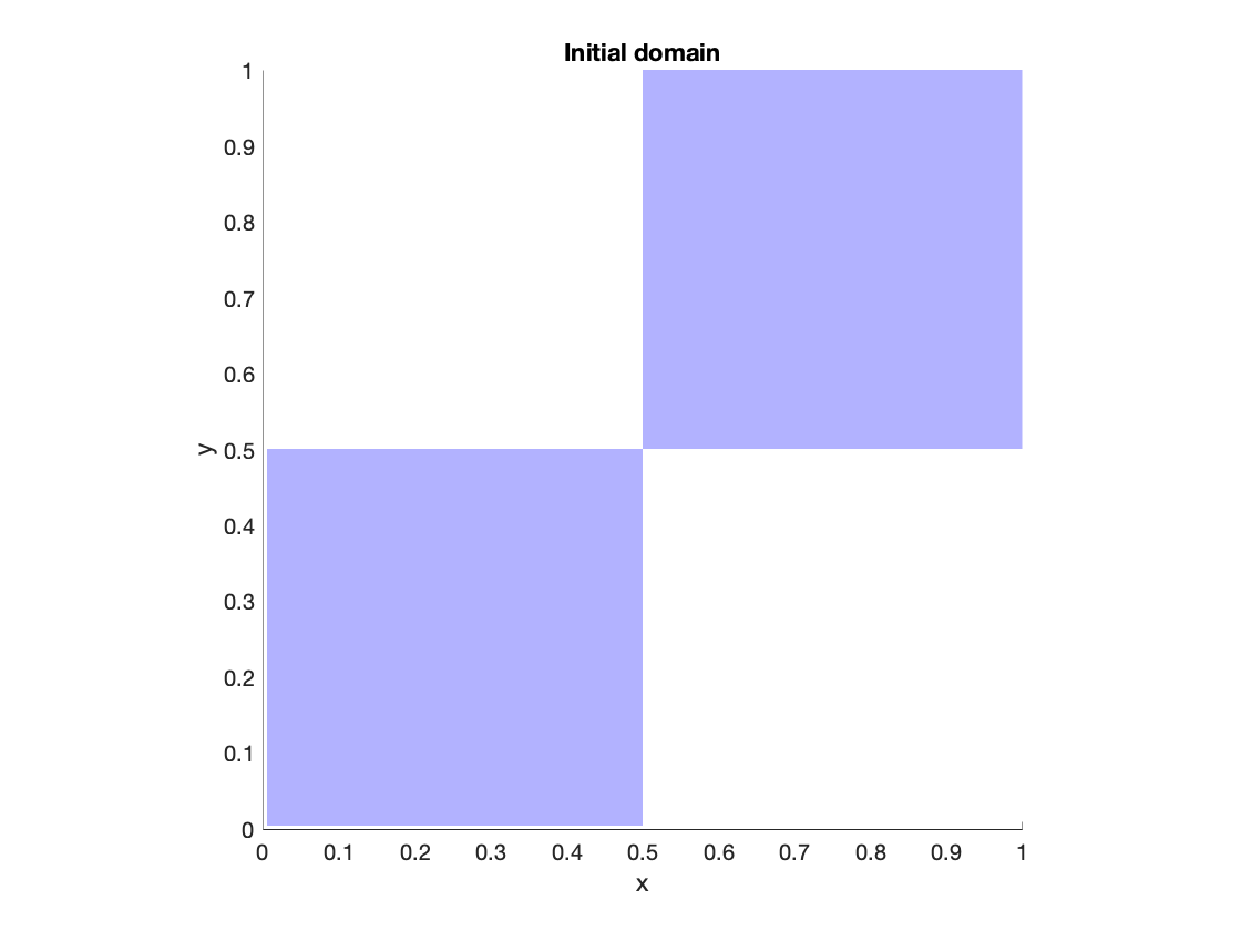
Figure 1: Domain $E_{0}$ chosen to initialize algorithm 3, i.e., $f_{0}=\mathds{1}_{E_{0}}$..

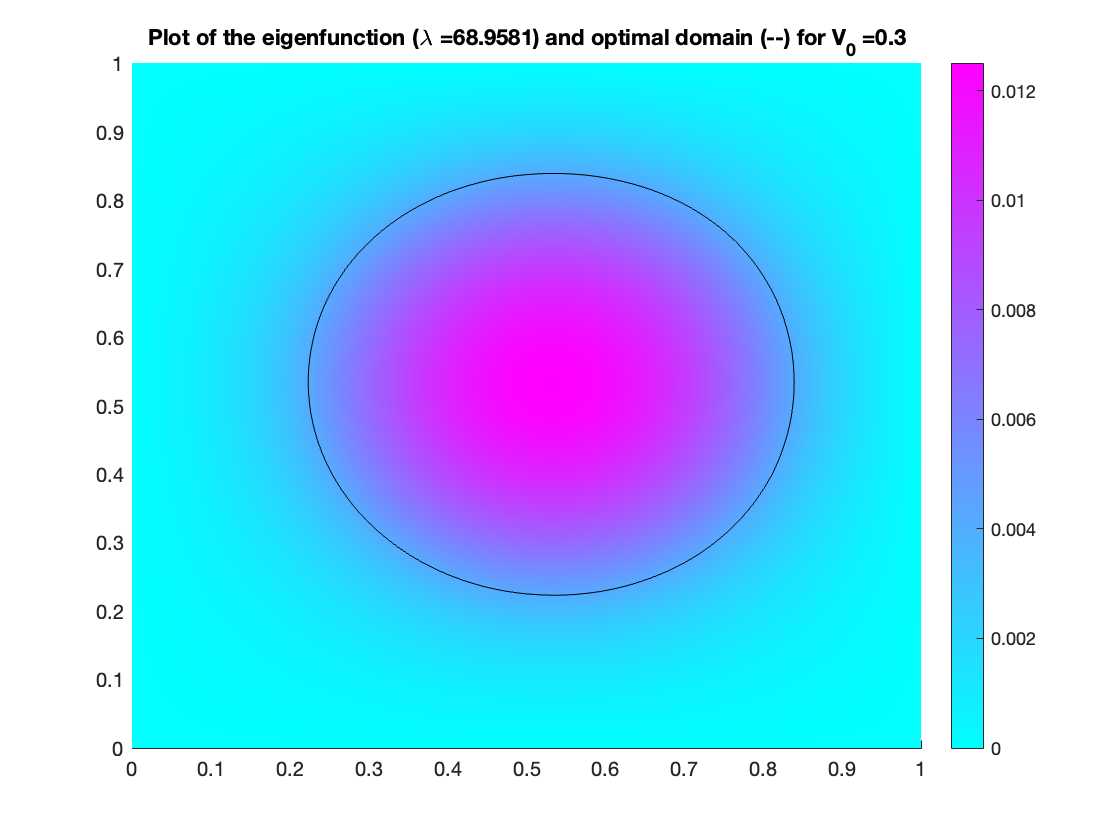
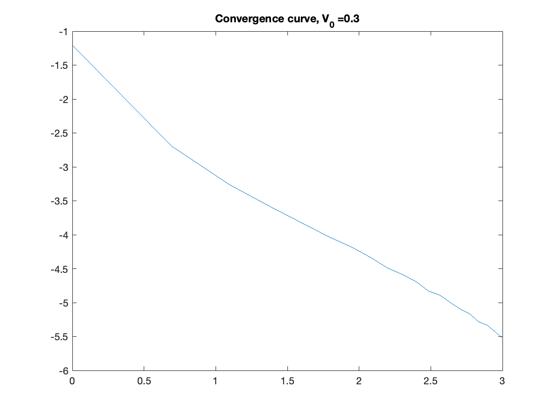
Figure 2: $V_{0}=0.3$. Left: representation of the optimal domain (black contour) and the eigenfunction (warmer colors indicate where the function takes its maximum values). Right: evolution of the quantity $\|f_{k+1}-f_{k}\|_{L^{1}(\Omega)}$ as a function of iterations, on a logarithmic scale.

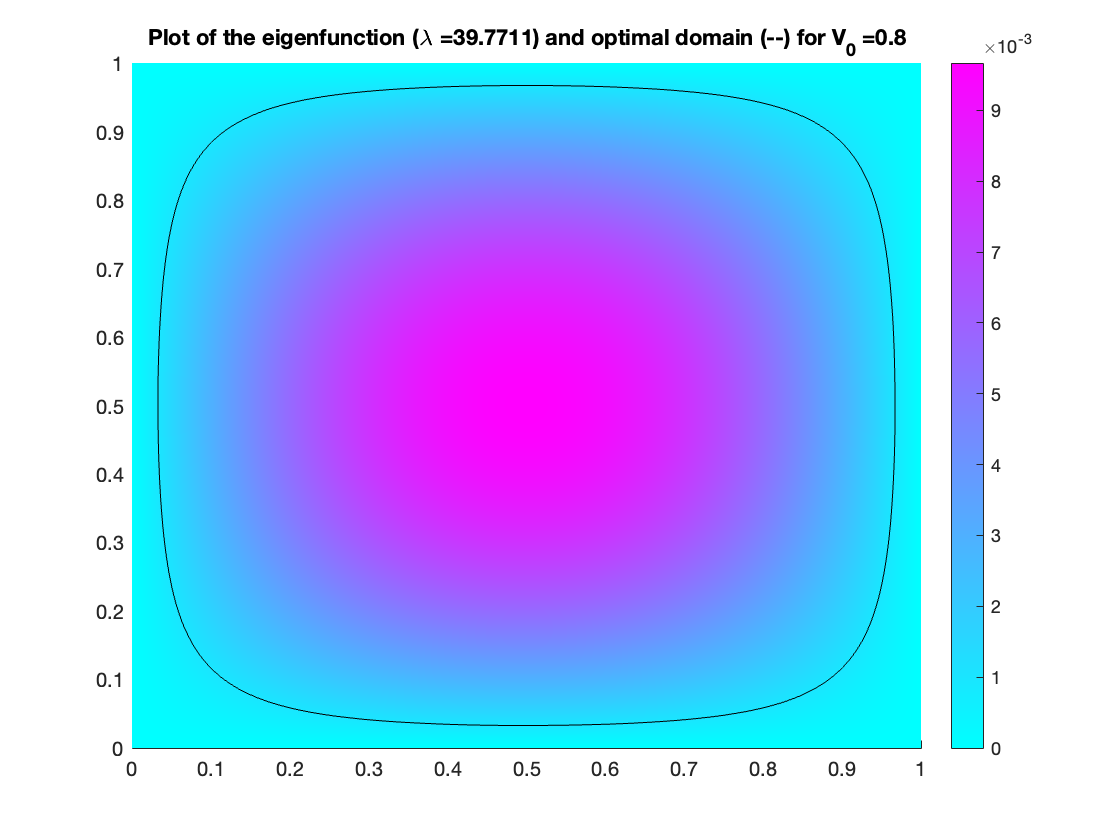
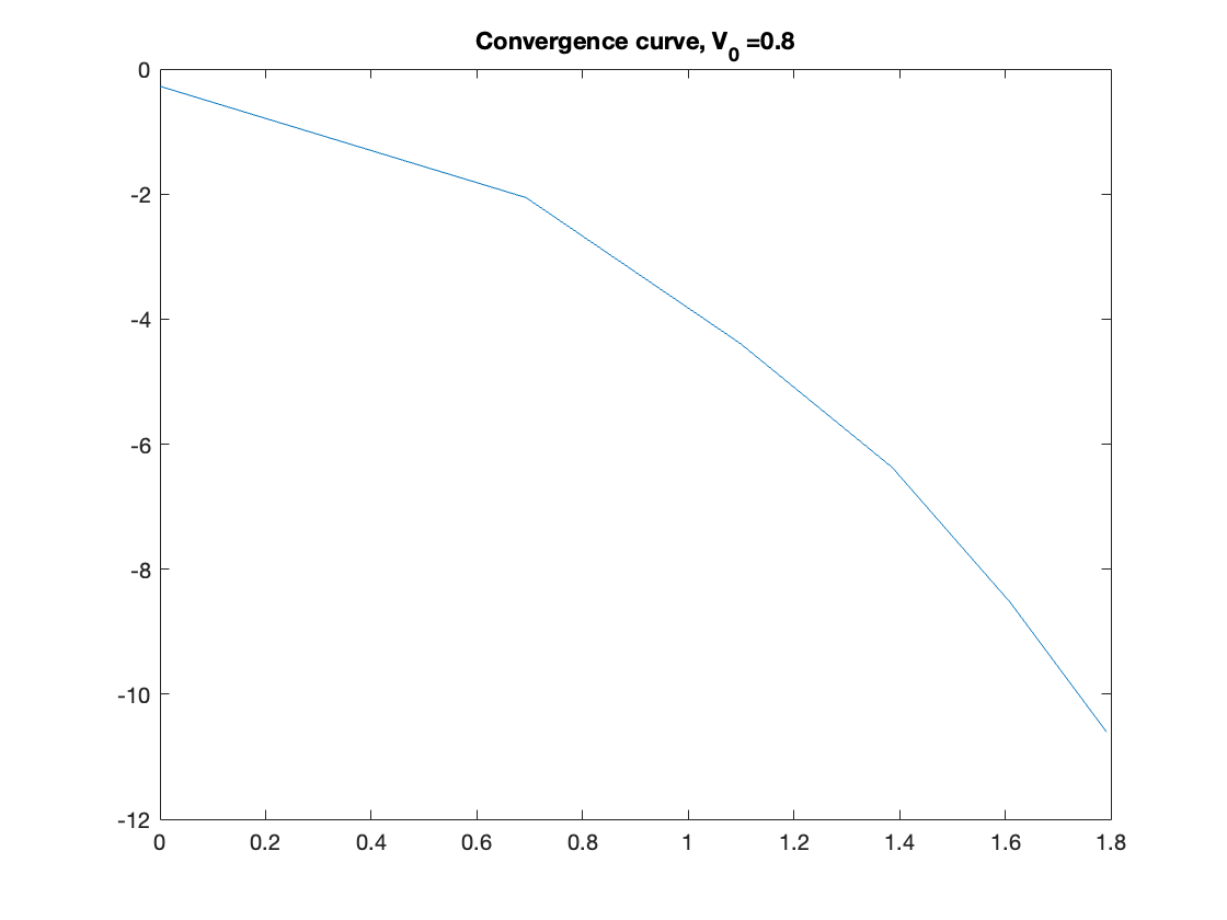
Figure 3: $V_{0}=0.8$. Left: representation of the optimal domain (black contour) and the eigenfunction (warmer colors indicate where the function takes its maximum values). Right: evolution of the quantity $\|f_{k+1}-f_{k}\|_{L^{1}(\Omega)}$ as a function of iterations, on a logarithmic scale.

1.5 Optimisation of non-energetic criteria

The functional and the optimal control problem.

The third and final problem we consider is the optimisation of a non-energetic criterion. We consider, for any $f\in\mathcal{F}(V_{0})$, the solution $u_{f}$ of the Dirichlet problem (1.1) (the same $u_{f}$ we used in the study of the Dirichlet energy). We fix a non-linearity $j=j(x,u)$ satisfying the following regularity assumptions:

$$\begin{cases}j\text{ is $\mathscr{C}^{2}$ in $u$, $\mathscr{C}^{1}$ in $x$}\,,\\ \text{For $k=0,1,2,i=0,1$, for any compact $K\subset\joinrel\subset\textnormal{I\kern-2.10007ptR}$ there holds }\underset{\overline{\Omega}\times K}{\sup}\|\partial_{x^{i}}^{i}\partial^{k}_{u^{k}}j\|_{L^{\infty}({\Omega})}<\infty\,,\\ \text{$j$ is strictly convex in $u$ and for any $u>0$ $\underset{\overline{\Omega}}{\inf}\partial^{2}_{u^{2}}j(x,u)>0$,}\\ \text{$j$ is increasing in $u$ for any $x\in\overline{\Omega}$, for any $u>0$, $\partial_{u}j(x,u)>0$.}\end{cases} \mathbb{H}_{j}$$ ()

The problem under consideration is

$$\framebox{$\displaystyle\max_{f\in\mathcal{F}(V_{0})}\left(J(f):=\int_{\Omega}j(x,u_{f}(x))dx\right).$} \mathbb{P}_{j}$$ ()

We start with a standard result.

Lemma 11.

The problem ($\mathbb{P}_{j}$) has a solution. Furthermore, the map $J$ is strictly convex. In particular any solution $f^{*}$ of ($\mathbb{P}_{\mathrm{Eigen}}$) is a bang-bang function in the sense of Definition 1: there exists $E^{*}\subset{\Omega}$ such that $f^{*}=\mathds{1}_{E^{*}}$, with $\mathrm{Vol}(E^{*})=V_{0}\mathrm{Vol}({\Omega}).$

The switch function and the thresholding algorithm.

We now describe the switch function in the following standard lemma:

Lemma 12.

The map $J$ is Fréchet-differentiable and, for any $f\in\mathcal{F}(V_{0})$, for any admissible perturbation $h$ at $f$ there holds

$$\dot{J}(f)[h]=\int_{\Omega}hp_{f}$$

where $p_{f}$ is the unique solution of

$$\begin{cases}-\Delta p_{f}=\partial_{u}j(x,u_{f})&\text{ in }{\Omega}\,,\\ p_{f}\in W^{1,2}_{0}({\Omega}).\end{cases}$$ (1.5)

Lemma 12 states that the function $p_{f}$ defined in (1.5) is the switch function of the optimal control problem ($\mathbb{P}_{j}$). This allows to describe the thresholding algorithm for ($\mathbb{P}_{j}$).

Algorithm 4 Thresholding algorithm for non-energetic problems eigenvalue

1:Initialisation at $f_{0}\in\mathcal{F}$

2:$k\leftarrow 0$

3:Compute $p_{f_{k}}$

4:Compute $c_{k}$ such that $\mathrm{Vol}(\{p_{f_{k}}>c_{k}\})=V_{0}\mathrm{Vol}({\Omega})$.

5:$f_{k}\leftarrow\mathds{1}_{\{p_{f_{k}}>c_{k}\}}$

6:$k\leftarrow k+1$.

Remark 6 applies here as well. The notion of “critical point” and of “local minimisers”, which were defined for the Dirichlet energy in Definitions 7-8, are identical for non-energetic criteria: it suffices to replace $\mathscr{E}$ with $J$.

Main result.

The main result regarding non-energetic problems is the following convergence theorem:

Theorem III.

Assume $j$ satisfies ($\mathbb{H}_{j}$). There exists ${\varepsilon}>0$ such that, if $1-{\varepsilon}\leqslant V_{0}<1$, for any initialisation $f_{0}\in\mathcal{F}(V_{0})$, the sequence $\{f_{k}\}_{k\in\textnormal{I\kern-1.47005ptN}}$ generated by Algorithm 4 converges strongly in $L^{1}({\Omega})$ to a local minimiser of $J$ in $\mathcal{F}(V_{0})$.

As it is very similar to the proof of Theorem I, the proof of Theorem III is given in [9, Section B].

1.6 The plan for the proof of convergence

As the schemes of proof for Theorems I, II and III are identical and as they are each quite long we now present the general plan. This allows use to single out the relevant elements for each step of the proof.

Consequence of the convexity of the functional.

The first part of the proof of convergence is to use the convexity or concavity properties of the functional (depending on whether we are maximising or minimising). To be more precise, consider a generic functional $\mathcal{G}:\mathcal{F}(V_{0})\to\textnormal{I\kern-2.10007ptR}$ that we seek to minimise in $\mathcal{F}(V_{0})$. Assume $\mathcal{G}$ is Fréchet-differentiable and denote by $-q_{f}$ its switch function at a given $f\in\mathcal{F}(V_{0})$ so that, for any $f$, for any admissible perturbation $h$ at $f$, there holds

$$\dot{\mathcal{G}}(f)[h]=-\int_{\Omega}q_{f}h.$$

Starting from $f_{k}$, we choose $f_{k+1}:=\mathds{1}_{\{q_{f_{k}}>c_{k}\}}$ where $\mathrm{Vol}\left(\{q_{f_{k}}>c_{k}\}\right)=V_{0}\mathrm{Vol}({\Omega})$. If the functional $\mathcal{G}$ is concave, then we have the estimate

$$\mathcal{G}(f_{k+1})-\mathcal{G}(f_{k})\leqslant\dot{\mathcal{G}}(f_{k})(f_{k+1}-f_{k})=-\int_{\Omega}q_{f_{k}}\left(f_{k+1}-f_{k}\right).$$ (1.6)

Thus we can be satisfied with gaining enough control of the first order derivative, which is a linear (in the perturbation $h$) functional.

Consequence of large volume constraints I: quantitative bathtub principle and well-posedness of thresholding algorithms.

This is where the large volume constraint plays a first role. Keeping the same notations as in the previous paragraph, observe that from Lemmata 5-10-12 the switch function $q_{f}$ satisfies a PDE with Dirichlet boundary conditions; as the PDEs involved enjoy a maximum principle, it is expected that, if $V_{0}$ is close enough to 1, then the set $\{q_{f}>c\}$ such that $\mathrm{Vol}(\{q_{f}>c\})=V_{0}$ is close to the boundary, and even $\mathscr{C}^{1}$ close to $\partial{\Omega}$. Moreover, it is expected that by elliptic regularity $q_{f}$ is $\mathscr{C}^{1,\alpha}$ close to $q_{\overline{f}\equiv 1}$, the function associated to $f=1$ (observe that when $V_{0}=1$ the set of admissible controls is reduced to a single point: $\mathcal{F}(V_{0})=\{\overline{f}\equiv 1\}$). Applying the Hopf Lemma to $q_{\overline{f}}$ we may get that, for $V_{0}$ close to 1, the gradient of $q_{f}$ is always non-zero in a neighbourhood of $\partial{\Omega}$. With these two informations combined, we deduce that the level set $\{q_{f}=c_{f}\}$ has zero measure and, hence, that the thresholding algorithm is indeed well defined.

But there is another crucial information we can deduce, and it is that $|{\nabla}q_{f}|\neq 0$ on $\{q_{f}=c_{f}\}$. Combined with the aforementioned regularity of the boundary we are then in a position to apply a quantitative bathtub principle [39, Proposition 26] (see also the related [14]). One information we have not yet given is that the choice of the next iterate $f_{k+1}$ in the thresholding algorithm is that $f_{k+1}$ is actually the unique maximiser of the functional

$$T:\mathcal{F}(V_{0})\ni f\mapsto\mapsto\int_{\Omega}q_{f_{k}}f.$$

With this notation (1.6) rewrites $\mathcal{G}(f_{k+1})-\mathcal{G}(f_{k})\leqslant T(f_{k})-T(f_{k+1})$. The quantitative bathtub principle writes: under certain regularity assumptions, for a certain constant $C>0$,

$$\forall f\in\mathcal{F}(V_{0})\,,T(f)-T(f_{k+1})\leqslant-C\|f_{k+1}-f\|_{L^{1}({\Omega})}^{2}.$$

Assuming that the constant $C$ is uniform in $k$ this would yield

$$G(f_{k+1})-G(f_{k})\leqslant-C\|f_{k+1}-f_{k}\|_{L^{1}({\Omega})}^{2}$$

and, in turn, prove that the sequence $\{f_{k}\}_{k\in\textnormal{I\kern-1.47005ptN}}$ satisfies $\sum_{k\in\textnormal{I\kern-1.47005ptN}}\|f_{k+1}-f_{k}\|_{L^{1}({\Omega})}^{2}<\infty$. Finally, we can prove that this implies that, either the sequence $\{f_{k}\}_{k\in\textnormal{I\kern-1.47005ptN}}$ converges, or it has an infinite number of closure points. To rule the latter possibility out, we use a shape derivation argument.

Consequence of large volume constraints II: shape derivative formalism and coercivity of shape hessians.

We use the shape derivative formalism of Hadamard; see [22, Chapter 5] for a full introduction. We can prove that any closure point of the sequence $\{f_{k}\}_{k\in\textnormal{I\kern-1.47005ptN}}$ is a bang-bang function $f^{*}=\mathds{1}_{E}$ that is also a critical point (in the sense that $\{q_{f^{*}}>c_{f^{*}}\}=E^{*}$). With an abuse of notation, for a bang-bang function $f=\mathds{1}_{E}$, we may define the shape functional

$$\mathcal{G}(E):=\mathcal{G}(\mathds{1}_{E}).$$

To show that possible closure points are isolated, which would allow to conclude, we prove that these closure points are stable in the sense of shapes [16]. Namely, considering a critical shape $E$ and smooth enough vector fields $\Phi$, we define shape Lagrangians (with a Lagrange multiplier $\mu=\mu(E^{*})$ independent of $\Phi$ and encoded by first order optimality conditions)

$$g_{\Phi}(t):=\mathcal{G}\left((\mathrm{Id}+t\Phi)E\right)+\mu\mathrm{Vol}\left((\mathrm{Id}+t\Phi)E\right)$$

so that $g^{\prime}(0)=0$. We then show a coercivity of second order shape derivatives or, in other words, that there exists a constant $C>0$ such that for any $\Phi$

$$g_{\Phi}^{\prime\prime}(0)\geqslant C\|\langle\Phi,\nu\rangle\|_{X(\partial E)}^{2}$$

for some norm $X$. In this case we say the second-order derivative is $X$-coercive. Our main contribution in this paper is to find a procedure to diagonalise these second order shape derivatives by using a new interior Steklov system of eigenvalues and eigenfunctions and to prove that, under large volume constraints, these second-order shape derivatives are indeed coercive with respect to the $L^{2}$-norm. We believe this is of independent interest. Once this is done we can apply the general procedure of [16], adapted in [35, 37, 39] to the setting of optimal control problems, to prove that critical points are isolated.

2 Proof of Theorem I

We begin with the study of ($\mathbb{P}_{\mathrm{Dir}}$).

2.1 First consequences of a large volume constraint

We gather here several crucial properties of the problem under large enough volume constraints. First, we show that when $V_{0}$ is close enough to 1 the level-sets generated by the thresholding algorithm enjoy strong regularity properties.

To state our results in a synthetic way we let, for any $f\in\mathcal{F}(V_{0})$, $\mu_{f,V_{0}}$ be the unique real number such that

$$\frac{\mathrm{Vol}(\{u_{f}>\mu_{f,V_{0}}\})}{\mathrm{Vol}({\Omega})}\leqslant V_{0}\leqslant\frac{\mathrm{Vol}(\{u_{f}\geqslant\mu_{f,V_{0}}\})}{\mathrm{Vol}({\Omega})}.$$

We also define

$$\omega_{f,V_{0}}:=\{u_{f}>\mu_{f,V_{0}}\}.$$

Lemma 13.

There exists ${\varepsilon}_{0}>0$ and $\delta_{0}>0$ such that, for any $V_{0}\in(1-{\varepsilon}_{0};1)$, for any $f\in\mathcal{F}(V_{0})$, we have on the one hand

$$\mathrm{Vol}(\{u_{f}=\mu_{f,V_{0}}\})=0$$

and, on the other hand, the following regularity properties:

1. $\omega_{f,V_{0}}$ has a $\mathscr{C}^{1,\alpha}$ boundary (for any $\alpha\in(0;1)$),

2. $$\min_{\partial\omega_{f,V_{0}}}\left|\frac{\partial u_{f}}{\partial\nu}\right|\geqslant\delta_{0},$$

3. $\partial\omega_{f,V_{0}}$ is locally a graph over $\partial{\Omega}$.

Finally, for any $\alpha\in(0;1)$, $\partial\omega_{f,V_{0}}$ converges to $\partial{\Omega}$ in $\mathscr{C}^{1,\alpha}$ as $V_{0}\to 1$, uniformly in $f\in\mathcal{F}(V_{0})$.

Proof of Lemma 13.

We will proceed in several steps.

Convergence to the torsion function. This lemma rests upon the study of the torsion function $w_{\Omega}$ of ${\Omega}$, defined as the solution of

$$\begin{cases}-\Delta w_{\Omega}=1&\text{ in }{\Omega}\,,\\ w_{\Omega}=0&\text{ on }\partial{\Omega}.\end{cases}$$ (2.1)

By the maximum principle of Hopf there exists $\underline{\delta}>0$ such that

$$\min_{\partial{\Omega}}\left|\frac{\partial w_{\Omega}}{\partial\nu}\right|\geqslant\underline{\delta}.$$ (2.2)

Furthermore, observe that standard $L^{p}$-regularity estimates (see for instance [20, Corollary 9.10]) entail that, for any $p\in[1;+\infty)$, there exists a constant $C_{p}>0$ such that for any $V_{0}\in(0;1)$ and any $f\in\mathcal{F}(V_{0})$

$$\|u_{f}\|_{W^{2,p}({\Omega})}\leqslant C_{p}.$$

From Sobolev embeddings, we deduce that for any $\alpha\in(0;1)$ there exists $H_{\alpha}$ such that for any $V_{0}\in(0;1)$ and any $f\in\mathcal{F}(V_{0})$

$$\|u_{f}\|_{\mathscr{C}^{1,\alpha}({\Omega})}\leqslant H_{\alpha}.$$ (2.3)

From these regularity estimates, we obtain at once the uniform convergence result

$$\forall\alpha\in(0;1)\,,\lim_{V_{0}\to 1}\sup_{f\in\mathcal{F}(V_{0})}\|u_{f}-w_{\Omega}\|_{\mathscr{C}^{1,\alpha}({\Omega})}=0.$$ (2.4)

Behaviour of $\mu_{f,V_{0}}$. Let us now prove that

$$\lim_{V_{0}\to 1}\sup_{f\in\mathcal{F}(V_{0})}|\mu_{f,V_{0}}|=0.$$ (2.5)

Argue by contradiction and assume (2.5) does not hold. Then there exist $\gamma>0$, a sequence $\{V_{k}\}_{k\in\textnormal{I\kern-1.47005ptN}}$ that satisfies $V_{k}\underset{k\to\infty}{\rightarrow}1$ and, for any $k\in\textnormal{I\kern-2.10007ptN}$, a function $f_{k}\in\mathcal{F}(V_{k})$ such that

$$\forall k\in\textnormal{I\kern-2.10007ptN}\,,|\mu_{f_{k},V_{0}}|\geqslant\gamma>0.$$ (2.6)

To obtain a contradiction, we first prove that there exists $\beta_{0}\,,{\varepsilon}_{0}^{\prime}\in(0;1)$ such that

$$\forall V_{0}\in(1-{\varepsilon}_{0}^{\prime};1)\,,\forall f\in\mathcal{F}(V_{0})\,,\beta_{0}w_{\Omega}\leqslant u_{f}\leqslant w_{\Omega}.$$

That $u_{f}\leqslant w_{\Omega}$ simply follows from the Hopf maximum principle as, for any $V_{0}\in(0;1)$ and any $f\in\mathcal{F}(V_{0})$ there holds $-\Delta u_{f}=f\leqslant 1=-\Delta w_{\Omega}$. Now fix $\beta_{0}\in(0;1)$. From (2.4) and (2.2) there exists ${\varepsilon}_{0}^{\prime}>0$ such that for any $V_{0}\in(1-{\varepsilon}_{0}^{\prime};1)$ and any $f\in\mathcal{F}(V_{0})$ we have

$$\beta_{0}\max_{\partial{\Omega}}\left|\frac{\partial w_{\Omega}}{\partial\nu}\right|<\min_{\partial{\Omega}}\left|\frac{\partial u_{f}}{\partial\nu}\right|.$$ (2.7)

As for any $\alpha\in(0;1)$ we have

$$w_{\Omega}\in\mathscr{C}^{1,\alpha}({\Omega})\,,\sup_{V_{0}\in(0;1)\,,{f\in\mathcal{V}_{0}}}\|u_{f}\|_{\mathscr{C}^{1,\alpha}({\Omega})}<\infty$$

we deduce that there exists $r_{0}^{\prime}>0$ small enough such that if we define

$$\Omega(r_{0}^{\prime}):=\left\{x\in{\Omega}\,,\mathrm{dist}(x,\partial{\Omega})\leqslant r_{0}^{\prime}\right\}$$ (2.8)

then (2.7) along with the Dirichlet boundary conditions implies

$$\beta_{0}w_{\Omega}\leqslant u_{f}\text{ in }{\Omega}(r_{0}^{\prime}).$$

From the maximum principle and (2.4) we also conclude that if ${\varepsilon}_{0}^{\prime}>0$ is small enough ($r_{0}^{\prime}>0$ being fixed) we have

$$\beta_{0}w_{\Omega}<u_{f}\text{ in }{\Omega}\backslash\Omega(r_{0}^{\prime}).$$

Thus we do obtain, if ${\varepsilon}_{0}^{\prime}>0$ is small enough that, for any $V_{0}\in(1-{\varepsilon}_{0}^{\prime};1)$, for any $f\in\mathcal{F}(V_{0})$ we have

$$\beta_{0}w_{\Omega}\leqslant u_{f}.$$ (2.9)

Let us now prove that (2.6) can not hold. From (2.9) we deduce that for any $k\in\textnormal{I\kern-2.10007ptN}$ we have

$$\left\{u_{f}\geqslant\mu_{f_{k},V_{k}}\right\}\subset\left\{w_{\Omega}\geqslant\frac{\mu_{f_{k},V_{k}}}{\beta_{0}}\right\}\subset\left\{w_{\Omega}\geqslant\frac{\gamma}{\beta_{0}}\right\}.$$

Consequently we deduce that

$$\forall k\in\textnormal{I\kern-2.10007ptN}\,,\mathrm{Vol}\left(\left\{u_{f}\geqslant\mu_{f_{k},V_{k}}\right\}\right)\leqslant\mathrm{Vol}\left(\left\{w_{\Omega}\geqslant\frac{\gamma}{\beta_{0}}\right\}\right)\leqslant 1-s_{0}$$

for a fixed $s_{0}\in(0;1)$, since $w_{\Omega}>0$ in ${\Omega}$ and $\gamma>0$. This is a contradiction with the definition of $\mu_{f_{k},V_{k}}$, whence the conclusion.

Study of $\omega_{f,V_{0}}$. From (2.2) and the fact that $w_{\Omega}\in\mathscr{C}^{1,\alpha}$ there exists $r_{0}>0$ such that

$$\left|{\nabla}w_{\Omega}\right|\geqslant\frac{\underline{\delta}}{2}\text{ in }{\Omega}(r_{0}^{\prime})$$

where ${\Omega}(r_{0})$ is defined in (2.8). Fix such an $r_{0}>0$. Since $w_{\Omega}>0$ in ${\Omega}$, (2.4)-(2.5) imply that there exists ${\varepsilon}_{0}^{\prime\prime}>0$ such that if $V_{0}\in(1-{\varepsilon}_{0}^{\prime\prime};1)$ then for any $f\in\mathcal{F}(V_{0})$

$$\{u_{f}=\mu_{f,V_{0}}\}\subset{\Omega}(r_{0}).$$

From (2.4) we also have, up to reducing ${\varepsilon}_{0}^{\prime\prime}>0$,

$$\inf_{V_{0}\in(1-{\varepsilon}_{0}^{\prime\prime};1)\,,f\in\mathcal{F}(V_{0})}\left(\inf_{{\Omega}(r_{0})}\left|{\nabla}u_{f}\right|\right)\geqslant\frac{\underline{\delta}}{4}.$$

From the implicit function theorem we deduce first that $\mathrm{Vol}\left(\{u_{f}=\mu_{f,V_{0}}\}\right)=0$, second that for any $\alpha\in(0;1)$, $\omega_{f,V_{0}}$ has a $\mathscr{C}^{1,\alpha}$ boundary and, finally, that there exists $\delta_{0}>0$ such that

$$\min_{\partial\omega_{f,V_{0}}}\left|\frac{\partial u_{f}}{\partial\nu}\right|\geqslant\delta_{0}.$$

Convergence of $\partial\omega_{f,V_{0}}$. We first prove that $\partial\omega_{f,V_{0}}$ is (locally) a graph over $\partial{\Omega}$. Argue by contradiction and assume that there exists a sequence $\{V_{k}\}_{k\in\textnormal{I\kern-1.47005ptN}}$ that converges to 1 and, for any $k\in\textnormal{I\kern-2.10007ptN}$, a function $f_{k}\in\mathcal{F}(V_{k})$, a sequence $\{x_{k}\}_{k\in\textnormal{I\kern-1.47005ptN}}\in\partial{\Omega}^{\textnormal{I\kern-1.47005ptN}}$ and two sequences $\{y_{k,0}\}_{k\in\textnormal{I\kern-1.47005ptN}}$, $\{y_{k,1}\}_{k\in\textnormal{I\kern-1.47005ptN}}$ of points of $\partial\omega_{f_{k},V_{k}}$ such that there exist $(t_{k,i})_{k\in\textnormal{I\kern-1.47005ptN}\,,i=0,1}\in(\textnormal{I\kern-2.10007ptR}_{+}\times\{0,1\})^{\textnormal{I\kern-1.47005ptN}}$ with

$$y_{k,i}=x_{k}-t_{k,i}\nu(x_{k})\,,t_{k,i}\underset{k\to\infty}{\rightarrow}0\,,t_{k,0}<t_{k,1}.$$

We consider a closure point $x_{\infty}$ of $\{x_{k}\}_{k\in\textnormal{I\kern-1.47005ptN}}$. By the intermediate value theorem, for any $k\in\textnormal{I\kern-2.10007ptN}$ there exists $s_{k}\in(t_{k,0};t_{k,1})$ such that, setting $z_{k}:=x_{k}-s_{k}\nu(x_{k})$ we have

$$\langle{\nabla}u_{f}(z_{k}),\nu(x_{k})\rangle=0.$$

Clearly we have $z_{k}\underset{k\to\infty}{\rightarrow}x_{\infty}$ and $\nu(x_{k})\underset{k\to\infty}{\rightarrow}\nu(x_{\infty})$. We obtain from (2.4)

$$\langle{\nabla}w_{\Omega}(x_{\infty})\,,\nu(x_{\infty})\rangle=0,$$

in contradiction with (2.2). Consequently, as $V_{0}\to 1$, for any $f\in\mathcal{F}(V_{0})$, $\partial\omega_{f,V_{0}}$ is a local graph over $\partial{\Omega}$; the fact that it converges to $\partial{\Omega}$ uniformly in $f\in\mathcal{F}(V_{0})$ is a simple consequence of (2.4).

∎

We note the following consequence of Lemma 13: if we denote by $\mathrm{Lip}(\Sigma)$ the Lipschitz-constant of a hypersurface $\Sigma$ then there exists ${\varepsilon}_{0}>0$ and a constant $M$ such that

$$\forall V_{0}\in(1-{\varepsilon}_{0};1)\,,\forall f\in\mathcal{F}(V_{0})\,,\mathrm{Lip}(\partial\omega_{f,V_{0}})+\mathrm{Per}(\omega_{f,V_{0}})\leqslant M.$$ (2.10)

We will use below [11, Lemma 3] to prove that $\omega_{f,V_{0}}$ actually has an analytic boundary, see Lemma 19; this is not necessary for the time being as we do not need analytic regularity.

We conclude with the following information about $\omega_{f,V_{0}}$.

Lemma 14.

There exists ${\varepsilon}_{0}^{\prime}>0$ such that, for any $V_{0}\in(1-{\varepsilon}_{0}^{\prime};1)$, for any $f\in\mathcal{F}(V_{0})$ the boundary $\partial\omega_{f,V_{0}}$ is connected.

Lemma 14.

We argue by contradiction. Then there exists a sequence $\{V_{k}\}_{k\in\textnormal{I\kern-1.47005ptN}}$ converging to 1 and, for any $k\in\textnormal{I\kern-2.10007ptN}$, a function $f_{k}\in\mathcal{F}(V_{k})$ such that $\partial\omega_{f_{k},V_{0}}$ has at least two connected components $\Sigma_{k,1}\,,\Sigma_{k,2}$. We pick, for any $k\in\textnormal{I\kern-2.10007ptN}$, two points $x_{k,i}\in\Sigma_{k,i}$ ($i=1,2$). First of all, for any closure point $y_{i}$ of the sequence $\{x_{k,i}\}_{k\in\textnormal{I\kern-1.47005ptN}}$ we have $y_{i}\in\partial{\Omega}$ ($i=1,2$). This is simply due to the fact that $u_{f_{k}}(x_{k,i})=\mu_{f_{k},V_{0}}\underset{k\to\infty}{\rightarrow}0$. Hence, from (2.4) we have $w_{\Omega}(y_{i})=0$, and we conclude by the maximum principle applied to the torsion function. Consequently, for $k$ large enough, $\partial\omega_{k,i}\subset{\Omega}(r_{0}^{\prime})$ where ${\Omega}(r_{0}^{\prime})$ is defined in (2.8) and $r_{0}^{\prime}$ is small enough to ensure that $\partial\omega_{f,V_{0}}$ is a graph over $\partial{\Omega}$. From the connectedness of $\partial{\Omega}$, we reach the desired contradiction. ∎

From the proof of this lemma we see that the only thing required is for $\partial\omega_{f,V_{0}}$ to be a graph over $\partial{\Omega}$ whence we may choose ${\varepsilon}_{0}={\varepsilon}_{0}^{\prime}$ where ${\varepsilon}_{0}$ is given in Lemma 13.

2.2 Applications of the quantitative bathtub principle

The first step of the proof is to apply the quantitative bathtub principle [39, Proposition 26] (see also [14]). Before we state this result in the form that will be used let us recall the bathtub principle [34, Theorem 1.14]: let $u\in\mathscr{C}^{0}({\Omega})$ and let $V_{0}\in(0;1)$ be such that there exists a unique $\mu_{u,V_{0}}$ such that

$$\mathrm{Vol}(\{u>\mu_{u,V_{0}}\})=V_{0}\mathrm{Vol}({\Omega})=\mathrm{Vol}(\{u\geqslant\mu_{u,V_{0}}\}).$$ (2.11)

If there exists a unique $\mu_{u,V_{0}}$ such that (2.11) is satisfied we define

$$\omega_{u,V_{0}}:=\left\{u>\mu_{u,V_{0}}\right\}.$$ (2.12)

Then:

$$f_{u}:=\mathds{1}_{\omega_{u,V_{0}}}\text{ is the unique solution of }\max_{f\in\mathcal{F}(V_{0})}\int_{\Omega}fu.$$ (2.13)

The goal of the quantitative bathtub principle is to quantify the optimality of $f_{u}$.

Proposition 15.

[39, Proposition 26] Let $\alpha\in(0;1)$. For any triplet of constants $M,P\,,\delta_{1}>0$ there exists a constant $c_{1}>0$ such that the following holds: for any function $u$ satisfying

1. there exists a unique $\mu_{u,V_{0}}$ that satisfies (2.11),

2. $\omega_{u,V_{0}}$ has a $\mathscr{C}^{1}$ boundary and

   $$\inf_{\partial\omega_{u,V_{0}}}\left|\frac{\partial u}{\partial\nu}\right|\geqslant\delta_{1}>0,$$

3. $\|u\|_{\mathscr{C}^{1,\alpha}({\Omega})}\leqslant M$ and $\mathrm{Per}(\omega_{u,V_{0}})\leqslant P,$

then, defining $f_{u}:=\mathds{1}_{\omega_{u,V_{0}}}$

$$\forall f\in\mathcal{F}(V_{0})\,,\int_{\Omega}fu\leqslant\int_{\Omega}f_{u}u-c_{1}\|f-f_{u}\|_{L^{1}({\Omega})}^{2}.$$ (2.14)

Application to the thresholding algorithm.

The goal of this paragraph is to apply Proposition 15 to the sequence generated by the thresholding algorithm.

Lemma 16.

Let ${\varepsilon}_{0},\delta_{0}$ be in the conditions of Lemma 13. For any $V_{0}\in(1-{\varepsilon}_{0};1)$, for any $f_{0}\in\mathcal{F}(V_{0})$, the sequence $\{f_{k}\}_{k\in\textnormal{I\kern-1.47005ptN}}$ is uniquely defined (in the sense that for any $k\in\textnormal{I\kern-2.10007ptN}$ there holds $\mathrm{Vol}\left(\{u_{f_{k}}=\mu_{f_{k},V_{0}}\}\right)=0$) and there holds

$$\sum_{k=0}^{\infty}\|f_{k+1}-f_{k}\|_{L^{1}({\Omega})}^{2}<\infty.$$ (2.15)

Proof of Lemma 16.

Let ${\varepsilon}_{0}\,,\delta_{0}$ in the conditions of Lemma 13. We fix $V_{0}\in(1-{\varepsilon}_{0};1)$. The fact that for any $k\in\textnormal{I\kern-2.10007ptN}$ we have

$$\mathrm{Vol}\left(\{u_{f_{k}}=\mu_{f_{k},V_{0}}\}\right)=0$$

is a conclusion of Lemma 13.

Since ${\Omega}$ is $\mathscr{C}^{2}$, by elliptic regularity, we know that for any $p\in[1;+\infty)$

$$\sup_{k\in\textnormal{I\kern-1.47005ptN}}\|u_{f_{k}}\|_{W^{2,p}({\Omega})}=M_{p}<\infty$$

whence from Sobolev embeddings [33, Theorem 12.5], fixing $s\in(0;1)$, we have

$$\sup_{k\in\textnormal{I\kern-1.47005ptN}}\|u_{f_{k}}\|_{\mathscr{C}^{1,s}({\Omega})}=:M<\infty.$$

Furthermore,

$$\inf_{k\in\textnormal{I\kern-1.47005ptN}}\min_{\partial\omega_{u_{f_{k}},V_{0}}}\left|\frac{\partial u_{f_{k}}}{\partial\nu}\right|\geqslant\delta_{0}>0.$$

Finally, estimate (2.10) allows us to apply Proposition 15 to deduce that there exists a constant $c_{1}>0$ such that

$$\forall k\in\textnormal{I\kern-2.10007ptN}\,,\int_{\Omega}u_{k}f_{k}\leqslant\int_{\Omega}u_{k}f_{k+1}-c_{1}\|f_{k+1}-f_{k}\|_{L^{1}({\Omega})}^{2}$$

or, equivalently,

$$\forall k\in\textnormal{I\kern-2.10007ptN}\,,c_{1}\|f_{k+1}-f_{k}\|_{L^{1}({\Omega})}^{2}\leqslant\int_{\Omega}u_{k}\left(f_{k+1}-f_{k}\right).$$ (2.16)

From the concavity of $\mathscr{E}$ (Lemma 4) we also know that

$$\forall k\in\textnormal{I\kern-2.10007ptN}\,,\mathscr{E}(f_{k+1})-\mathscr{E}(f_{k})\leqslant\dot{\mathscr{E}}(f_{k})[f_{k+1}-f_{k}]=\int_{\Omega}u_{k}\left(f_{k}-f_{k+1}\right).$$

Thus we obtain

$$\forall k\in\textnormal{I\kern-2.10007ptN}\,,c_{1}\|f_{k+1}-f_{k}\|_{L^{1}({\Omega})}^{2}\leqslant\mathscr{E}(f_{k})-\mathscr{E}(f_{k+1}).$$ (2.17)

However, there exists $\underline{E}$ such that

$$\forall V_{0}\in(0;1)\,,\forall f\in\mathcal{F}(V_{0})\,,\underline{E}\leqslant\mathscr{E}(f).$$ (2.18)

This is a direct consequence of the variational formulation of the Dirichlet energy (1.2). Summing the estimates (2.17) for $k\in\textnormal{I\kern-2.10007ptN}$ we get

$$c_{1}\sum_{k=0}^{\infty}\|f_{k+1}-f_{k}\|_{L^{1}({\Omega})}^{2}\leqslant\mathscr{E}(f_{0})-\underline{E}<\infty.$$

As $c_{1}>0$, the proof is concluded. ∎

The purpose of this lemma is to give us more insight into the possible asymptotic behaviours of $\{f_{k}\}_{k\in\textnormal{I\kern-1.47005ptN}}$. We detail this in the next paragraph.

Let us start with a basic lemma:

Lemma 17.

Let ${\varepsilon}_{0}$ be in the conditions of Lemma 13. For any $V_{0}\in(1-{\varepsilon}_{0};1)$, for any initialisation $f_{0}\in\mathcal{F}(V_{0})$, any $L^{\infty}-*$ closure point $f_{\infty}$ of the sequence $\{f_{k}\}_{k\in\textnormal{I\kern-1.47005ptN}}$ generated by the thresholding algorithm is a bang-bang function:

$$\exists E_{\infty}\subset{\Omega}\,,f_{\infty}=\mathds{1}_{E_{\infty}}.$$ (2.19)

Furthermore $E_{\infty}=\{u_{f_{\infty}}>\mu_{u_{f_{\infty}},V_{0}}\}$, which is uniquely defined. In other words, $E_{\infty}$ is a critical set in the sense of Definition 7.

Proof of Lemma 17.

We do not relabel the $L^{\infty}-*$ converging subsequence and write it $\{f_{k}\}_{k\in \textnormal{I\kern-1.47005ptN}}$; its closure point is called $f_{\infty}$. We recall that ${\varepsilon}_{0}$ is given by Lemma 13. By elliptic regularity, for any $p\in[1;+\infty)$,

$$\sup_{k\in\textnormal{I\kern-1.47005ptN}}\|u_{f_{k}}\|_{W^{2,p}({\Omega})}<\infty.$$

By Sobolev embeddings, for any $\alpha\in(0;1)$,

$$u_{f_{k}}\underset{k\to\infty}{\overset{\mathscr{C}^{1,\alpha}({\Omega})}{\longrightarrow}}u_{f_{\infty}}.$$

Define, for any $k\in\textnormal{I\kern-2.10007ptN}$, $\omega_{k}:=\{u_{f_{k}}\geqslant\mu_{u_{f_{k}},V_{0}}\}$. From (2.10) we deduce that $\{\omega_{k}\}_{k\in\textnormal{I\kern-1.47005ptN}}$ satisfies a uniform ${\varepsilon}$-cone property ([22, Remark 2.4.8]). From [22, Theorem 2.4.10] the sequence $\{\omega_{k}\}_{k\in\textnormal{I\kern-1.47005ptN}}$ converges in the $L^{1}$-topology to a measurable subset $\omega_{\infty}$ of ${\Omega}$, with $\mathrm{Vol}(\omega_{\infty})=V_{0}\mathrm{Vol}({\Omega})$; as $f_{k+1}=\mathds{1}_{\omega_{k}}$ we deduce that $f_{\infty}=\mathds{1}_{\omega_{\infty}}$. Moreover, still from [22, Theorem 2.4.10] the sequence $\{\partial\omega_{k}\}_{k\in\textnormal{I\kern-1.47005ptN}}$ converges to $\partial\omega_{\infty}$ in the Hausdorff distance. Consequently, passing to the limit in $\partial\omega_{k}=\{u_{f_{k}}=\mu_{f_{k},V_{0}}\}$ we deduce that $u_{f_{\infty}}$ is constant on $\partial\omega_{\infty}$. $\omega_{\infty}$ is thus necessarily the superlevel set of $u_{f_{\infty}}$ with volume $V_{0}$, which concludes the proof.

∎

Using this result we can provide a simplification of the behaviour of the sequence $\{f_{k}\}_{k\in\textnormal{I\kern-1.47005ptN}}$.

Lemma 18.

Let ${\varepsilon}_{0}$ be chosen as in Lemma 13. For any $V_{0}\in(1-{\varepsilon}_{0};1)$, for any initialisation $f_{0}\in\mathcal{F}(V_{0})$, let $\{f_{k}\}_{k\in\textnormal{I\kern-1.47005ptN}}$ be the sequence generated by the thresholding algorithm. Then:

1. Either $\{f_{k}\}_{k\in\textnormal{I\kern-1.47005ptN}}$ has a unique weak $L^{\infty}-*$ closure point $f_{\infty}$, in which case $f_{k}\underset{k\to\infty}{\rightarrow}f_{\infty}$ strongly in $L^{1}({\Omega})$,

2. Or $\{f_{k}\}_{k\in\textnormal{I\kern-1.47005ptN}}$ has an infinite number of closure points.

Proof of Lemma 18.

Observe that if $\{f_{k}\}_{k\in\textnormal{I\kern-1.47005ptN}}$ has a weak $L^{\infty}-*$ closure point $f_{\infty}$, Lemma 17 ensures that $f_{\infty}$ is an extreme point of $\mathcal{F}(V_{0})$, whereby $f_{\infty}$ is actually a strong $L^{1}$ closure point of the sequence.

We prove that if the sequence $\{f_{k}\}_{k\in\textnormal{I\kern-1.47005ptN}}$ has two distinct closure points $f_{\infty,1}\neq f_{\infty,2}$, then it has infinitely many closure points. First of all, from Lemma 16,

$$\|f_{k+1}-f_{k}\|_{L^{1}({\Omega})}\underset{k\to\infty}{\rightarrow}0.$$ (2.20)

By Lemma 17 there exist $F_{\infty}^{1}\,,F_{\infty}^{2}\subset{\Omega}$ such that

$$f_{\infty,i}=\mathds{1}_{F_{\infty,i}}\quad(i=1,2).$$

Let $\delta_{1}\in(0;\mathrm{dist}_{L^{1}}(F_{\infty,1},F_{\infty,2})/4)$ and define

$$\textnormal{I\kern-2.10007ptN}_{1}:=\{k\in\textnormal{I\kern-2.10007ptN}:\min_{i=1,2}(\|f_{k}-f_{\infty,i}\|_{L^{1}({\Omega})})\geqslant\delta_{1}\}.$$

From (2.20), $\textnormal{I\kern-2.10007ptN}_{1}$ is infinite. We denote it as

$$\textnormal{I\kern-2.10007ptN}_{1}=\{i_{0},\dots,i_{k},\dots\}.$$

The sequence $\{f_{i_{k}}\}_{k\in\textnormal{I\kern-1.47005ptN}}$ contains an $L^{\infty}-*$ converging subsequence, still denoted by $\{f_{i_{k}}\}_{k\in\textnormal{I\kern-1.47005ptN}}$. Let $f_{\infty,3}$ be its closure point and let us show that

$$\min_{i=1,2}(\|f_{\infty,3}-f_{\infty,i}\|_{L^{1}({\Omega})})\geqslant\delta_{1}.$$

We only show

$$\|f_{\infty,3}-f_{\infty,1}\|_{L^{1}({\Omega})}\geqslant\delta_{1}$$ (2.21)

as the same proof would yield that $\|f_{\infty,3}-f_{\infty,2}\|_{L^{1}({\Omega})}\geqslant\delta_{1}$. To prove (2.21) we use in a crucial manner that $f_{\infty,1}$ is a bang-bang function (see Definition 1). Consider $h_{k}:=f_{i_{k}}-f_{\infty,1}$. Then we have

$$h_{k}=h_{k,+}\mathds{1}_{F_{\infty,1}^{c}}-h_{k,-}\mathds{1}_{F_{\infty,1}}$$

with $h_{k,\pm}\geqslant 0$. This is a simple consequence of the fact that $f_{\infty,1}$ is bang-bang. Furthermore, we have

$$\int_{F_{\infty,1}^{c}}h_{k,+}+\int_{F_{\infty,1}}h_{k,-}\geqslant\delta.$$

We consider a weak closure point $h_{\infty,+}$ of $\{h_{k,+}\mathds{1}_{F_{\infty,1}^{c}}\}_{k\in\textnormal{I\kern-1.47005ptN}}$ and a weak closure point $h_{\infty,-}$ of $\{h_{k,-}\mathds{1}_{F_{\infty,1}}\}_{k\in\textnormal{I\kern-1.47005ptN}}$. We obtain

$$\int_{F_{\infty,1}^{c}}h_{\infty,+}+\int_{F_{\infty,1}}h_{\infty,-}\geqslant\delta.$$

Furthermore, by linearity of the weak convergence we have

$$f_{\infty,3}-f_{\infty,1}=h_{\infty,+}\mathds{1}_{F_{\infty,1}^{c}}-h_{\infty,-}\mathds{1}_{F_{\infty,1}}.$$

Consequently

$$\|f_{\infty,3}-f_{\infty,1}\|_{L^{1}({\Omega})}\geqslant\delta,$$

whence the conclusion. Thus we deduce that (2.21) holds and, adapting the reasoning for $f_{\infty,2}$, we obtain that

$$\min_{i=1,2}\left(\|f_{\infty,3}-f_{\infty,i}\|_{L^{1}({\Omega})}\right)\geqslant\delta.$$

By Lemma 17, $f_{\infty,3}$ is a bang-bang function, and $\{f_{k}\}_{k\in\textnormal{I\kern-1.47005ptN}}$ has three distinct closure points. It then suffices to iterate the procedure to construct an infinite sequence of closure points. This concludes the proof.∎

The goal of the next sections.

To obtain the uniqueness of the closure point and the strong convergence to a local minimiser, we need to show that every critical point (in the sense of Definition 7) is actually a local minimiser and that these critical points are isolated. This is done using shape derivatives and diagonalisation of shape hessians.

2.3 Qualitative study of critical points

In this section we give an in-depth analysis of critical points (in the sense of Definition 7). We begin with the analyticity of the boundaries of critical sets.

Regularity of critical sets.

We will be using a shape derivative formalism and compute second order shape derivatives at critical shapes in order to conclude as to their minimality and to obtain a full convergence result for the thresholding algorithm. Doing so requires some regularity (at least $\mathscr{C}^{3}$ for second-order shape derivatives) of the boundary of critical sets. It should be noted that usually this type of regularity is proved for minimal sets (i.e. for $E\subset{\Omega}$ such that $\mathds{1}_{E}$ is a solution of ($\mathbb{P}_{\mathrm{Dir}}$)). A paradigmatic result is the regularity of minimal sets in two dimensions [13]. However, the hard part in proving this regularity is usually obtaining an estimate of the gradient of the state function on the boundary of the optimal set. Working with a large volume constraint allows to bypass this regularity problem, as gradient estimates are readily provided by Lemma 13, and thus enable us to apply [11, Lemma 3, Theorem 8].

Lemma 19.

Let ${\varepsilon}_{0}>0$ be as in Lemma 13. Any critical set $E$ (in the sense of Definition 7) has a compact analytic boundary and, furthermore, is uniformly bounded in the $\mathscr{C}^{2}$ topology.

Proof of Lemma 19.

This proof is an adaptation of [11, Proof of Theorem 8]. Let us first recall the following simpler version of [11, Lemma 3]:

Lemma 20 (Lemma 3, [11]).

Let $h:\textnormal{I\kern-2.10007ptR}\to\textnormal{I\kern-2.10007ptR}$ be a locally bounded function and $w\in\mathscr{C}^{1}({\Omega})$ be a solution of

$$\Delta w=h(w)\text{ in }{\Omega}.$$

Let $x_{0}\in{\Omega}$ be such that ${\nabla}w(x_{0})\neq 0$. There exists a ball $\mathbb{B}(x_{0};r)$ ($r>0$) such that the set $\{x\in{\mathbb{B}}:\,w(x)=w(x_{0})\}$ is an analytic hypersurface of $\textnormal{I\kern-2.10007ptR}^{d}$.

The original version of [11, Lemma 3] also features a dependency of $h$ on ${\nabla}w$; this is not necessary here. Now consider a critical set $E\subset{\Omega}$. Let $u_{\mathds{1}_{E}}$ be the solution of (1.1) with $f=\mathds{1}_{E}$ and let $\mu_{E}$ be such that

$$E=\{u_{\mathds{1}_{E}}>\mu_{E}\}.$$ (2.22)

The fact that (2.22) holds follows from Lemma 13. Defining the (locally bounded) function $h:\eta\mapsto\mathds{1}_{(\mu_{E};+\infty)}(\eta)$, we thus have

$$-\Delta u_{\mathds{1}_{E}}=h(u_{\mathds{1}_{E}}).$$

From Lemma 13, for any $x_{0}\in\partial E=\{x:\,u_{\mathds{1}_{E}}(x)=\mu_{E}\}$, we have

$${\nabla}u_{\mathds{1}_{E}}(x_{0})\neq 0.$$

Applying Lemma 20 we deduce that $\partial E$ is locally analytic. In other words, we may write

$$\partial E=\underset{x\in\partial E}{\bigcup}({\mathbb{B}}(x;r_{x})\cap\partial E)$$

with $r_{x}>0$ for any $x\in\partial E$ and ${\mathbb{B}}(x;r_{x})\cap\partial E$ is an analytic hypersurface of $\textnormal{I\kern-2.10007ptR}^{n}$. As $\partial E$ is compact by continuity of $u_{\mathds{1}_{E}}$, we may extract a finite covering of $\partial E$ and hence conclude that $\partial E$ is a compact analytic hypersurface. To obtain the uniform $\mathscr{C}^{2}$ bounds it suffices to conclude as in [11, Lemma 3, Theorem 8], by using (2.10). ∎

Preliminary considerations about shape derivatives at critical shapes.

We first identify the functional $\mathscr{E}$ with a shape functional $\mathscr{F}$, by defining

$$\mathscr{F}:{\Omega}\supset E\mapsto\mathscr{E}(\mathds{1}_{E}).$$

For any compact $\mathscr{C}^{3}$ subset $E$ of ${\Omega}$ and for any compactly supported vector field $\Phi\in W^{2,\infty}({\Omega};\textnormal{I\kern-2.10007ptR}^{d})$, we can define, for any $t\in(-1;1)$ small enough, the function

$$e_{E,\Phi}(t):=\mathscr{F}\Big{(}(\mathrm{Id}+t\Phi)E\Big{)}.$$

Provided they exists, the first (resp. second) order derivative of $\mathscr{F}$ at $E$ in the direction $\Phi$ is defined as

$$\mathscr{F}^{\prime}(E)[\Phi]=e_{E,\Phi}^{\prime}(0)\,,\text{resp. }\mathscr{F}^{\prime\prime}(E)[\Phi,\Phi]=e_{E,\Phi}^{\prime\prime}(0).$$

We first check that $\mathscr{E}$ is indeed twice differentiable in the sense of shapes.

Lemma 21.

For any $\mathscr{C}^{3}$ subset $E$ of ${\Omega}$, $\mathscr{F}$ is twice differentiable at $E$ in the direction of any compactly supported vector-field $\Phi\in W^{2,\infty}({\Omega};\textnormal{I\kern-2.10007ptR}^{d})$.

As this lemma is proved by a direct adaptation of [41] we omit it here and focus in a subsequent paragraph on the computation of first and second order shape derivatives.

First order shape derivative and definition of the Lagrange multiplier.

In terms of optimality conditions, since we are working with volume constraints, we have to work with the shape derivative of the volume functional. We recall [22, Section 5.9.3, first example] that the map

$${\Omega}\supset E\mapsto\mathrm{Vol}(E)$$

is twice shape differentiable (i.e. differentiable in the direction of any compactly supported vector field $\Phi\in W^{2,\infty}({\Omega})$) at any $\mathscr{C}^{3}$ domain $E$ and that, for any compactly supported vector field $\Phi$, there holds

$$\mathrm{Vol}^{\prime}(E)[\Phi]=\int_{\partial E}\langle\Phi,\nu_{E}\rangle\,,\mathrm{Vol}^{\prime\prime}(E)[\Phi,\Phi]=\int_{\partial E}\mathscr{H}_{E}\langle\Phi,\nu\rangle^{2}$$ (2.23)

where $\nu_{E}$ is the normal vector on $\partial E$ and $\mathscr{H}_{E}$ is the mean curvature of $\partial E$.

For semantical convenience, we introduce the following definition:

Definition 22 (Critical shape).

A $\mathscr{C}^{2}$ shape $E$ is a critical shape for $\mathscr{F}$ if, for any compactly supported $\Phi\in W^{2,\infty}({\Omega})$,

$$\int_{\partial E}\langle\Phi,\nu_{E}\rangle=0\Rightarrow\mathscr{F}^{\prime}(E)[\Phi]=0.$$

In order to exploit second order optimality conditions it is more convenient to use a Lagrange multiplier. If a shape $E$ is critical, then the condition given in Definition 22 rewrites as: there exists a constant $\mu_{E}$ such that, for any compactly supported vector field $\Phi\in W^{2,\infty}({\Omega};\textnormal{I\kern-2.10007ptR}^{d})$,

$$\left(\mathscr{F}+\mu_{E}\mathrm{Vol}\right)^{\prime}(E)[\Phi]=0.$$ (2.24)

Computing this Lagrange multiplier is an important step in our subsequent analysis; to do it we need an expression of the first order derivative.

Lemma 23.

For any $\mathscr{C}^{3}$ shape, for any compactly supported vector field $\Phi\in W^{2,\infty}({\Omega};\textnormal{I\kern-2.10007ptR}^{d})$,

$$\mathscr{F}^{\prime}(E)[\Phi]=-\int_{\partial E}u_{\mathds{1}_{E}}\langle\Phi,\nu_{E}\rangle.$$

Furthermore, the shape derivative of the map $E\mapsto u_{\mathds{1}_{E}}$ at $E$ in the direction $\Phi$ is the unique solution of

$$\begin{cases}-\Delta u_{\Phi}^{\prime}=0&\text{ in }{\Omega}\,,\\ \left\llbracket\partial_{\nu}u_{\Phi}^{\prime}\right\rrbracket=-\langle\Phi,\nu_{E}\rangle&\text{ on }\partial E\end{cases}$$ (2.25)

where $\llbracket\cdot\rrbracket$ denotes the jump of a function across a hypersurface.

Proof of Lemma 23.

To prove this lemma we first need to compute the shape derivative of the map $u\mapsto u_{\mathds{1}_{E}}$. These computations were already carried out (for the shape derivative of the first eigenvalue of the operator $-\Delta-\mathds{1}_{E}$) in details in [39], but we sketch them in the present case for the sake of completeness. Fix $E$ and a compactly supported vector field $\Phi$. Define, for any $t$ such that $|t|$ small enough, $E_{t}:=\mathds{1}_{(\mathrm{Id}+t\Phi)E}$ and $u_{t}$ as the solution of (1.1) with $f=\mathds{1}_{E_{t}}$. The weak formulation of the equation on $u_{t}$ reads:

$$\forall v\in W^{1,2}_{0}({\Omega})\,,\int_{\Omega}\langle{\nabla}u_{t},{\nabla}v\rangle=\int_{E_{t}}v.$$ (2.26)

Taking the derivative of this formulation at $t=0$, it appears that the shape derivative $u_{\Phi}^{\prime}$ satisfies the equation

$$\forall v\in W^{1,2}_{0}({\Omega})\,,\int_{\Omega}\langle{\nabla}u_{\Phi}^{\prime},{\nabla}v\rangle=\int_{\partial E}v\langle\Phi,\nu_{E}\rangle.$$ (2.27)

Alternatively, this rewrites as: $u_{\Phi}^{\prime}$ is the unique solution of the equation

$$\begin{cases}-\Delta u_{\Phi}^{\prime}=0&\text{ in }{\Omega}\,,\\ \left\llbracket\partial_{\nu}u_{\Phi}^{\prime}\right\rrbracket=-\langle\Phi,\nu_{E}\rangle&\text{ on }\partial E\end{cases}$$

exactly as claimed in the statement of the theorem. Now, going back to the definition of $\mathscr{F}$ we obtain

$$\mathscr{F}^{\prime}(E)[\Phi]=\int_{\Omega}\langle{\nabla}u_{\mathds{1}_{E}},{\nabla}u_{\Phi}^{\prime}\rangle-\int_{E}u_{\Phi}^{\prime}-\int_{\partial E}u_{\mathds{1}_{E}}\langle\Phi,\nu_{E}\rangle.$$

Using the weak formulation of (1.1) this gives

$$\mathscr{F}^{\prime}(E)[\Phi]=-\int_{\partial E}u_{\mathds{1}_{E}}\langle\Phi,\nu_{E}\rangle.$$

∎

This expression allows us to prove the following result

Lemma 24.

A shape $E\subset{\Omega}$ is a critical set in the sense of Definition 7 if, and only if it is a critical shape in the sense of Definition 22.

Proof of Lemma 24.

Let us first notice that from Lemma 19, critical shapes in the sense of Definition 7 are analytic and thus in particular $\mathscr{C}^{2}$.

Consider now a critical point $E$ in the sense of Definition 7. By definition there exists a constant $\mu_{E}$ such that $u_{\mathds{1}_{E}}=\mu_{E}$ on $\partial E$. As $E$ is $\mathscr{C}^{2}$ from Lemma 19 we can legitimately compute the first order shape derivative of $\mathscr{F}$ at $E$ in the direction of a fixed compactly supported vector field $\Phi$. By Lemma 23

$$\mathscr{F}^{\prime}(E)[\Phi]=-\int_{\partial E}u_{\mathds{1}_{E}}\langle\Phi,\nu_{E}\rangle=-\mu_{E}\int_{\partial E}\langle\Phi,\nu_{E}\rangle.$$

Hence, if $\int_{\partial E}\langle\Phi,\nu_{E}\rangle=0$ we have $\mathscr{F}^{\prime}(E)[\Phi]=0$ and thus $E$ is a critical shape in the sense of Definition 22.

Conversely, consider a shape $E$ of class $\mathscr{C}^{3}$ that is critical in the sense of Definition 22. As for any compactly supported vector field $\Phi$ such that $\int_{\partial E}\langle\Phi,\nu_{E}\rangle=0$ we must have

$$\int_{\partial E}u_{\mathds{1}_{E}}\langle\Phi,\nu_{E}\rangle=0$$

the fundamental lemma of the calculus of variations implies the existence of a constant $\mu_{E}>0$ such that

$$u_{\mathds{1}_{E}}=\mu_{E}\text{ on }\partial E.$$

From the maximum principle applied to (1.1) we already know that $u_{\mathds{1}_{E}}>0$ in ${\Omega}$, hence $\mu_{E}>0$. Consequently $\partial E\cap\partial{\Omega}=\emptyset$ and $u_{\mathds{1}_{E}}$ is a solution of

$$\begin{cases}-\Delta u_{\mathds{1}_{E}}=1&\text{ in }E\,,\\ u_{E}=\mu_{E}&\text{ on }\partial E\end{cases}\text{ and }\begin{cases}-\Delta u_{\mathds{1}_{E}}=0&\text{ in }{\Omega}\backslash\overline{E}\,,\\ u_{\mathds{1}_{E}}=\mu_{E}&\text{ on }\partial E\,,\\ u_{\mathds{1}_{E}}=0&\text{ on }\partial{\Omega}.\end{cases}$$ (2.28)

As $\partial E\cap\partial{\Omega}=\emptyset$, both $E$ and ${\Omega}\backslash\overline{E}$ are smooth open sets. From the strong maximum principle we deduce that $u_{\mathds{1}_{E}}>\mu_{E}$ in $E$ and that $u_{\mathds{1}_{E}}<\mu_{E}$ in ${\Omega}\backslash\overline{E}$. Thus $E$ is a critical set in the sense of Definition 7. ∎

From this analysis we deduce the following:

Lemma 25.

Assume $E$ is a critical shape in the sense of Definition 22. The associated Lagrange multiplier is $\mu_{E}$ where $E=\{u_{\mathds{1}_{E}}>\mu_{E}\}$ in the sense that

$$\forall\Phi\in W^{2,\infty}({\Omega};\textnormal{I\kern-2.10007ptR}^{d})\,,\Phi\text{ compactly supported }\,,\left(\mathscr{F}+\mu_{E}\mathrm{Vol}\right)^{\prime}(E)[\Phi]=0.$$

To alleviate notations we introduce a notation for the shape Lagrangian:

Definition 26 (Shape Lagrangian).

Let $E$ be a critical shape for $\mathscr{F}$. The associated shape Lagrangian is

$$\mathscr{L}_{E}:=\mathscr{F}+\mu_{E}\mathrm{Vol}$$

where $E=\{u_{\mathds{1}_{E}}>\mu_{E}\}$.

With the above ingredients at hand, we now move to second-order shape derivatives.

First computations and elements for shape hessians.

In the subsequent paragraphs we use indifferently the expressions ”shape hessians” and ”second order shape derivatives”. We begin with an expression of the shape hessian at a critical shape $E$ in the direction $\Phi$.

Lemma 27.

Let $E$ be a critical shape in the sense of Definition 22 and let $\Phi\in W^{2,\infty}({\Omega};\textnormal{I\kern-2.10007ptR}^{d})$ be a compactly supported vector field. The second-order shape derivative of the shape Lagrangian $\mathscr{L}_{E}$ (defined in Definition 26) is given by the expression

$$\mathscr{L}_{E}^{\prime\prime}(E)[\Phi,\Phi]=-\int_{\partial E}u_{\Phi}^{\prime}\langle\Phi,\nu_{E}\rangle-\int_{\partial E}\frac{\partial u_{E}}{\partial\nu}\langle\Phi,\nu_{E}\rangle^{2}$$

where $u_{\Phi}^{\prime}$ solves (2.25).

Proof of Lemma 27.

First of all, since $E$ is a critical shape, it suffices to work with vector fields that are normal to $\partial E$ (see [22, Remark on page 246]). We recall that the formula of Hadamard gives

$$\left.\frac{d}{dt}\right|_{t=0}\int_{\Gamma(t)}f(t)=\int_{\Gamma(0)}f^{\prime}(0)+\int_{\Gamma(0)}\left(\mathscr{H}_{\Gamma(0)}f+\frac{\partial f}{\partial\nu}\right)\langle\Phi,\nu\rangle$$

where $\mathscr{H}_{\cdot}$ denotes the mean curvature of a hypersurface.

Let us start from the fact that, at a given shape $E$ we have (Lemma 23)

$$\mathscr{F}^{\prime}(E)[\Phi]=-\int_{\partial E}u_{\mathds{1}_{E}}\langle\Phi,\nu_{E}\rangle.$$

Applying the formula of Hadamard we obtain

$$\mathscr{F}^{\prime\prime}(E)[\Phi,\Phi]=-\int_{\partial E}u_{\Phi}^{\prime}\langle\Phi,\nu\rangle-\int_{\partial E}\left(\mathscr{H}_{E}u_{\mathds{1}E}+\frac{\partial u_{\mathds{1}_{E}}}{\partial\nu}\right)\langle\Phi,\nu_{E}\rangle^{2}.$$

Taking into account the definition of the Lagrange multiplier (Lemma 25) and (2.23) we finally derive the following expression for the second-order shape derivative of the Lagrangian (see Definition 26)

$$\mathscr{L}_{E}^{\prime\prime}(E)[\Phi,\Phi]=-\int_{\partial E}u_{\Phi}^{\prime}\langle\Phi,\nu\rangle-\int_{\partial E}\frac{\partial u_{\mathds{1}_{E}}}{\partial\nu}\langle\Phi,\nu_{E}\rangle^{2}.$$ (2.29)

∎

The question of coercivity of shape Lagrangians.

The goal of upcoming sections is to provide coercivity results on shape Lagrangians at critical shapes. By coercivity we mean not only that the shape hessian is positive, i.e. that for any compactly supported vector field $\Phi\in W^{2,\infty}({\Omega};\textnormal{I\kern-2.10007ptR}^{d})$ we have

$$\mathscr{L}_{E}^{\prime\prime}(E)[\Phi,\Phi]>0\text{ whenever }\langle\Phi,\nu_{E}\rangle\neq 0\text{ on }\partial E$$

but that we can even quantify this positivity, in the sense that there exists a constant $c_{E}>0$ (independent of $\Phi$) such that

$$\mathscr{L}_{E}^{\prime\prime}(E)[\Phi,\Phi]\geqslant c_{E}\|\langle\Phi,\nu_{E}\rangle\|_{L^{2}(\partial E)}^{2}.$$

This leads to introducing the following definition:

Definition 28 ($L^{2}$-stability).

A critical shape $E$ is said to be $L^{2}$-stable if there exists a constant $c_{E}>0$ such that for any compactly supported vector field $\Phi\in W^{2,\infty}({\Omega};\textnormal{I\kern-2.10007ptR}^{d})$,

$$\mathscr{L}_{E}^{\prime\prime}(E)[\Phi,\Phi]\geqslant c_{E}\|\langle\Phi,\nu_{E}\rangle\|_{L^{2}(\partial E)}^{2}.$$

It should be noted that we can not expect a better coercivity norm than $L^{2}(\partial E)$; when diagonalising the shape hessian we actually will prove the optimality of this norm. While weaker than the usual $H^{\frac{1}{2}}(\partial E)$ norm [16, 17, 23] this is still enough to obtain local quantitative inequalities [39].

Our goal is henceforth to prove the following coercivity result:

Proposition 29.

There exists ${\varepsilon}_{1}>0\,,{\varepsilon}_{1}\leqslant{\varepsilon}_{0}\,,\underline{c}>0$ such that, for any $V_{0}\in(1-{\varepsilon}_{1};1)$, for any critical set $E$ (in the sense of Definition 22), for any compactly supported vector field $\Phi\in W^{2,\infty}({\Omega};\textnormal{I\kern-2.10007ptR}^{d})$,

$$\mathscr{L}_{E}^{\prime\prime}(E)[\Phi,\Phi]\geqslant\underline{c}\|\langle\Phi,\nu\rangle\|_{L^{2}(\partial E)}^{2}.$$

Before we prove this proposition we need to introduce the diagonalisation basis. We consider a fixed critical shape $E\subset{\Omega}$ and work with $V_{0}\in(1-{\varepsilon}_{0};1)$, where ${\varepsilon}_{0}$ is given by Lemma 13. Heuristically, given that $u_{\Phi}^{\prime}$ satisfies (2.25), it is natural to solve the following eigenvalue problem: find $(\lambda,\phi)\in\textnormal{I\kern-2.10007ptR}\times W^{1,2}({\Omega})$ such that

$$\begin{cases}-\Delta\phi=0&\text{ in }E\cup\left(E\right)^{c}\\ \llbracket\partial_{\nu}\phi\rrbracket_{E}=-\lambda\rho\phi&\text{ on }\partial E\,,\\ \int_{\partial E}\phi^{2}>0\,,\\ \phi\in W^{1,2}_{0}({\Omega})\end{cases}$$ (2.30)

where $\rho$ is a weight to be determined. Let us simply consider the eigenvalue problem (2.30) with a weight $\rho\in L^{\infty}(\partial E;[\delta,1/\delta])$ for some small $\delta>0$. To study this spectral problem we introduce the weighted space

$$L^{2}_{\rho}(\partial E):=\left\{f\in L^{2}(\partial E),\int_{\partial E}\rho f^{2}<\infty\right\}=L^{2}(\partial E).$$

The last equality comes from the fact that the weight $\rho$ is uniformly bounded. The only difference here is of course the scalar product; we work with

$$\langle\cdot,\cdot\rangle_{\rho}:(f,g)\mapsto\int_{\partial E}\rho fg.$$

Under these assumptions it is fairly standard to obtain the existence of a spectral basis associated with (2.30). Define the operator $T_{\rho}:L^{2}_{\rho}(\partial E)\to L^{2}(\partial E)$ as follows: for any $f\in L^{2}_{\rho}(\partial E)$ let $v_{f}\in W^{1,2}({\Omega})$ be the unique solution to

$$\begin{cases}-\Delta v_{f}=0&\text{ in }{\Omega}\,,\\ \llbracket\partial_{\nu}v_{f}\rrbracket=-\rho f&\text{ on }\partial E\,,\\ v_{f}\in W^{1,2}_{0}({\Omega}).\end{cases}$$ (2.31)

The fact that for any $f\in L^{2}_{\rho}(\partial E)$ the function $v_{f}$ exists and is unique simply follows by minimising the functional

$$W_{\rho,f}:W^{1,2}_{0}({\Omega})\ni v\mapsto\frac{1}{2}\int_{\Omega}|{\nabla}v|^{2}-\int_{\partial E}\rho vf.$$

Let $\mathrm{Tr}_{E}:W^{1,2}({\Omega})\to L^{2}(\partial E)$ be the trace operator. As $E$ is analytic (Lemma 19) this operator is well-defined. Set

$$T_{\rho}(f):=\mathrm{Tr}_{E}(v_{f}).$$ (2.32)

In particular,

$$\forall f\in L^{2}_{\rho}(\partial E)\,,T_{\rho}(f)\in L^{2}_{\rho}(\partial E).$$

Clearly, $T_{\rho}$ is symmetric, positive and compact. In particular, by the spectral decomposition theorem, there exists a sequence of eigen-elements $\left\{\left(\sigma_{k,\rho}\,,\psi_{k,\rho}\right)\right\}_{k\in\textnormal{I\kern-1.47005ptN}}\in\left(\textnormal{I\kern-2.10007ptR}_{+}^{*}\times L^{2}_{\rho}(\partial E)\right)^{\textnormal{I\kern-1.47005ptN}}$ such that

$$\sigma_{k,\rho}\text{ is non-increasing in $k$ and }\sigma_{k,\rho}\underset{k\to\infty}{\longrightarrow}0,$$

$$\{\psi_{k,\rho}\}_{k\in\textnormal{I\kern-1.47005ptN}}\text{ is an orthonormal basis of $L^{2}_{\rho}(\partial E)$}$$

and

$$\forall k\in\textnormal{I\kern-2.10007ptN}\,,\quad T_{\rho}(\psi_{k,\rho})=\sigma_{k,\rho}\psi_{k,\rho}.$$

We set $\phi_{k,\rho}:=v_{\psi_{k,\rho}}$ to extend it to a function on ${\Omega}$. Hence,

$$\begin{cases}-\Delta\phi_{k,\rho}=0&\text{ in }{\Omega}\,,\\ \llbracket\partial_{\nu}\phi_{k,\rho}\rrbracket=-\rho\psi_{k,\rho}=-\frac{1}{\sigma_{k,\rho}}\rho\phi_{k,\rho}&\text{ on }\partial E\,,\\ \phi_{k,\rho}=0&\text{ on }\partial{\Omega}.\end{cases}$$ (2.33)

We thus obtain, defining

$$\lambda_{k,\rho}:=\frac{1}{\sigma_{k,\rho}}$$

the system

$$\forall k\in\textnormal{I\kern-2.10007ptN}^{*}\,,\begin{cases}-\Delta\phi_{k,\rho}=0&\text{ in }{\Omega}\,,\\ \llbracket\partial_{\nu}\phi_{k,\rho}\rrbracket=-\lambda_{k,\rho}\rho\phi_{k,\rho}&\text{ on }\partial E\,,\\ \phi_{k,\rho}=0&\text{ on }\partial{\Omega}\end{cases}\\ \text{ and }\forall k\,,k^{\prime}\in\textnormal{I\kern-2.10007ptN}^{*}\,,\int_{\partial E}\rho\phi_{k,\rho}\phi_{k^{\prime},\rho}=\delta_{k,k^{\prime}}.$$ (2.34)

The family $\{\phi_{0,\rho}\}\cup\{\phi_{k,\rho}\}_{k\in\textnormal{I\kern-1.47005ptN}^{*}}=\{\phi_{k,\rho}\}_{k\in\textnormal{I\kern-1.47005ptN}}$ is an orthonormal basis of $L^{2}_{\rho}(\partial E)$ for the scalar product $\langle\cdot,\cdot\rangle_{\rho}$.

From the Courant-Fisher principle we have, furthermore, the following characterisation of the first eigenvalue:

$$\lambda_{0,\rho}=\min_{u\in W^{1,2}_{0}({\Omega})\,,\int_{\partial E}u^{2}>0}\frac{\int_{\Omega}|{\nabla}u|^{2}}{\int_{\partial E}\rho u^{2}}.$$ (2.35)

Diagonalisation of $\mathscr{L}_{E}^{\prime\prime}(E)$.

We can now turn back to the expression of the second-order shape derivative of the Lagragian (2.29). We want to determine the weight $\rho$. We use the following notational convention: for any $\Phi\in W^{2,\infty}({\Omega};\textnormal{I\kern-2.10007ptR}^{d})$,

$${\varphi}:=\langle\Phi\,,\nu\rangle\,,\tilde{\varphi}:=\frac{1}{\rho}{\varphi}.$$

The first-order shape derivative $u_{\Phi}^{\prime}$ satisfies

$$\begin{cases}-\Delta u_{\Phi}^{\prime}=0&\text{ in }{\Omega}\,,\\ \left\llbracket\frac{\partial u_{\Phi}^{\prime}}{\partial\nu}\right\rrbracket=-\rho\tilde{\varphi}&\text{ on }\partial E\,,\\ u_{\Phi}^{\prime}=0&\text{ on }\partial{\Omega}.\end{cases}$$ (2.36)

We decompose $\tilde{\varphi}$ in the basis $\{\phi_{k,\rho}\}_{k\in\textnormal{I\kern-1.47005ptN}}$ as

$$\tilde{\varphi}=\sum_{k=0}^{\infty}\alpha_{k,\rho}\phi_{k,\rho}.$$ (2.37)

Thus,

$$u_{\Phi}^{\prime}=\sum_{k=0}^{\infty}\frac{\alpha_{k,\rho}}{\lambda_{k,\rho}}\phi_{k,\rho}.$$

As a conclusion

$$\mathscr{L}_{E}^{\prime\prime}(E)[\Phi,\Phi] =-\int_{\partial E}u_{\Phi}^{\prime}\langle\Phi\,,\nu_{E}\rangle-\int_{\partial E}\partial_{\nu}u_{\mathds{1}_{E}}\langle\Phi,\nu_{E}\rangle^{2}$$

$$=-\int_{\partial E}\rho\tilde{\varphi}u_{\Phi}^{\prime}-\int_{\partial E}\rho^{2}\partial_{\nu}u_{\mathds{1}_{E}}\left(\tilde{\varphi}\right)^{2}.$$

Let us choose

$$\rho_{E}=-\frac{1}{\partial_{\nu}u_{\mathds{1}_{E}}}.$$

From Lemma 13, we have $\rho_{E}\in L^{\infty}([\delta;1/\delta])$ for $\delta$ small enough. Finally, this yields

$$\mathscr{L}_{E}^{\prime\prime}(E)[\Phi,\Phi] =-\int_{\partial E}u_{\Phi}^{\prime}\langle\Phi\,,\nu_{E}\rangle-\int_{\partial E}\partial_{\nu}u_{\mathds{1}_{E}}\langle\Phi,\nu_{E}\rangle^{2}$$

$$=-\int_{\partial E}\rho_{E}\tilde{\varphi}u_{\Phi}^{\prime}-\int_{\partial E}\rho_{E}^{2}\partial_{\nu}u_{\mathds{1}_{E}}\left(\tilde{\varphi}\right)^{2}$$

$$=\sum_{k=0}^{\infty}\alpha_{k,\rho_{E}}^{2}\left(1-\frac{1}{\lambda_{k,\rho_{E}}}\right).$$

In particular, given that the sequence $\{\lambda_{k,\rho_{E}}\}_{k\in\textnormal{I\kern-1.47005ptN}}$ is non-decreasing, we have the estimate from below:

$$\mathscr{L}_{E}^{\prime\prime}(E)[\Phi,\Phi]\geqslant\left(1-\frac{1}{\lambda_{0,\rho_{E}}}\right)\sum_{k=0}^{\infty}\alpha_{k,\rho_{E}}^{2}=\left(1-\frac{1}{\lambda_{0,\rho_{E}}}\right)\|\langle\Phi,\nu_{E}\rangle\|_{L^{2}(\partial E)}^{2}.$$ (2.38)

Hence we have the following sufficient condition for the stability of a critical shape:

Lemma 30.

If $\lambda_{0,\rho_{E}}>1$, then $E$ is stable in the sense of Definition 28.

To prove Proposition 29 we study the asymptotic behaviour of $\lambda_{0,\rho_{E}}$ as $V_{0}\to 1$.

Asymptotic behaviour of $\lambda_{0,\rho_{E}}$ as $V_{0}\to 1$.

We prove here the following lemma:

Lemma 31.

There holds

$$\min_{E\text{ critical shape for the volume constraint $V_{0}$}}\lambda_{0,E}\underset{V_{0}\to 1}{\rightarrow}\infty.$$

Remark 32 (Heuristic approach to Lemma 31).

Assume ${\Omega}=(-1;1)$ and $V_{0}=1-{\varepsilon}$, where ${\varepsilon}>0$ is a small parameter. In this case, we may use the Schwarz rearrangement to obtain that the unique solution of ($\mathbb{P}_{\mathrm{Dir}}$) is $f^{*}=\mathds{1}_{I_{\varepsilon}}$ where

$$I_{\varepsilon}=(-1+{\varepsilon}/2;1-{\varepsilon}/2).$$

Let $u_{\varepsilon}$ be the associated solution of (1.1). Clearly,

$$u_{\varepsilon}\underset{{\varepsilon}\to 0}{\rightarrow}u_{0}$$

in $\mathscr{C}^{1}({\Omega})$, where $u_{0}$ is the solution of (1.1) with $f\equiv 1$. In particular,

$$|u_{\varepsilon}^{\prime}(\pm 1\mp{\varepsilon}/2)|=a_{\varepsilon}\underset{{\varepsilon}\to 0}{\rightarrow}1.$$

Now let us study the lowest eigenvalue $\lambda_{0,\rho_{I_{\varepsilon}}}$ which, for the sake of notational convenience, we rewrite as $\lambda_{0}({\varepsilon})$. But notice the following thing: if we define

$${\varphi}_{0,{\varepsilon}}:x\mapsto\begin{cases}1\text{ if }|x|\leqslant 1-{\varepsilon}/2,\\ \frac{2}{{\varepsilon}a_{\varepsilon}}(1-|x|)\text{ if }1-{\varepsilon}/2\leqslant|x|\leqslant 1\end{cases}$$

it appears that ${\varphi}_{0,{\varepsilon}}$ is an eigenfunction associated with the eigenvalue $\frac{2}{{\varepsilon}}$. As it has a constant sign, and as the eigenfunction associated with the lowest eigenvalue is the only one that has a constant sign, we deduce that

$$\lambda_{0,\rho_{I_{\varepsilon}}}({\varepsilon})=\frac{2}{{\varepsilon}},$$

which indeed goes to $\infty$ as ${\varepsilon}\to 0^{+}$.

The situation is of course more complicated in higher dimensions. Here is a roadmap to prove the same type of results. We already observed in the proof of Lemma 13 that $u_{f}\underset{V_{0}\to 1}{\rightarrow}w$ uniformly in $f$, as ${\varepsilon}\to 0$, where $w$ is the torsion function of the set ${\Omega}$. As ${\Omega}$ has a regular boundary, the Hopf maximum principle entails that

$$\inf_{\partial{\Omega}}\left(-\frac{\partial w}{\partial\nu}\right)=\delta({\Omega})>0.$$

Now consider the set $X^{*}_{\varepsilon}$ of critical shapes. From the definition of criticality, it follows that, for any $E^{*}\in X^{*}$, there exists $\mu(E^{*})$ such that $E^{*}=\{u_{\mathds{1}_{E^{*}}}>\mu(E^{*})\}$. We want to prove that

$$\lim\inf_{{\varepsilon}\to 0^{+}}\min_{E^{*}\in X^{*}_{\varepsilon}}\lambda_{0,\rho_{E^{*}}}=+\infty.$$

We argue by contradiction and assume this is not the case. This gives a sequence ${\varepsilon}\to 0^{+}$ and a sequence $\{E_{\varepsilon}\}_{{\varepsilon}>0}\in\prod_{{\varepsilon}>0}X^{*}_{\varepsilon}$ such that

$$\sup_{\varepsilon}\lambda_{0,\rho_{E^{*}}}\leqslant M_{0}<\infty.$$

By Lemma 13, $E^{*}_{\varepsilon}$ converges in $\mathscr{C}^{1,\alpha}$ to ${\Omega}$ (for any $\alpha<1$). Now observe that, in fact, by a standard comparison principle, we may be satisfied to prove that $\lambda({\varepsilon})\to\infty$ where $\lambda({\varepsilon})$ is defined as

$$\lambda({\varepsilon}):=\inf_{{\varphi}\in W^{1,2}_{0}({\Omega})}\frac{\int_{\Omega}|{\nabla}{\varphi}|^{2}}{\int_{\partial E_{\varepsilon}}{\varphi}^{2}}.$$

This follows from the lower bound on $|\partial_{\nu}u_{\varepsilon}|$ given by Lemma 13. The idea is then that, if the eigenvalues are uniformly bounded, then we should have on the one-hand (up to renormalisation)

$$\int_{E_{\varepsilon}}{\varphi}_{\varepsilon}^{2}=1$$

and, on the other hand, we should have enough regularity on ${\varphi}_{\varepsilon}$ to write

$$\int_{E_{\varepsilon}}{\varphi}_{\varepsilon}^{2}\sim\int_{\partial{\Omega}}{\varphi}_{\varepsilon}^{2}=0.$$

This would be an obvious contradiction.

Proof of Lemma 31.

We first observe that from Lemma 13 and the Rayleigh quotient formulation (2.35) of $\lambda_{0,\rho_{E}}$ we have, for $V_{0}\in(1-{\varepsilon}_{0};{\varepsilon})$,

$$\lambda_{0,\rho_{E}}\geqslant\delta_{0}\min_{u\in W^{1,2}_{0}({\Omega})\,,\int_{\partial E}u^{2}\neq 0}\frac{\int_{\Omega}|{\nabla}u|^{2}}{\int_{\partial E}u^{2}}.$$

Now, argue by contradiction and assume that there exists a sequence ${\varepsilon}\to 0$, a constant $M_{0}>0$, and, for any ${\varepsilon}>0$, a critical set $E_{\varepsilon}$ such that $\mathds{1}_{E_{\varepsilon}}\in\mathcal{F}(V_{0})$ with $V_{0}\in(1-{\varepsilon};1)$ that satisfies

$$\lambda_{0,\rho_{E_{\varepsilon}}}\leqslant M_{0}.$$

Define, for any ${\varepsilon}>0$,

$$\lambda({\varepsilon}):=\min_{u\in W^{1,2}_{0}({\Omega})\,,\int_{\partial E_{\varepsilon}}u^{2}\neq 0}\frac{\int_{\Omega}|{\nabla}u|^{2}}{\int_{\partial E_{\varepsilon}}u^{2}}.$$

As already observed we have $\delta_{0}\lambda({\varepsilon})\leqslant\lambda_{0,\rho_{E_{\varepsilon}}}$ so that the sequence $\{\lambda({\varepsilon})\}_{{\varepsilon}\to 0}$ is uniformly bounded. In other words we have

$$0<\lambda({\varepsilon})\leqslant M_{1}<\infty$$ (2.39)

for some suitable constant $M_{1}$. We define, for any ${\varepsilon}>0$, ${\varphi}_{\varepsilon}$ as the first eigenfunction associated with $\lambda({\varepsilon})$; in other words, ${\varphi}_{\varepsilon}$ solves the equation

$$\begin{cases}-\Delta{\varphi}_{\varepsilon}=0&\text{ in }{\Omega}\,,\\ \left\llbracket\frac{\partial{\varphi}_{\varepsilon}}{\partial\nu}\right\rrbracket=-\lambda({\varepsilon}){\varphi}_{\varepsilon}&\text{ on }\partial E_{\varepsilon}\,,\\ {\varphi}_{\varepsilon}\in W^{1,2}_{0}({\Omega})\,,\\ \int_{\partial E_{\varepsilon}}{\varphi}_{\varepsilon}^{2}=1.\end{cases}$$ (2.40)

Let us prove that if (2.39) holds then:

$$\forall\beta\in(0;1)\,,\exists c_{\beta}\,,\sup_{{\varepsilon}>0}\|{\varphi}_{\varepsilon}\|_{\mathscr{C}^{0,\beta}}\leqslant c_{\beta}.$$ (2.41)

First of all, from the uniform regularity estimates of Lemma 13 and from [33, Theorem 18.34], for any $p\in(1;+\infty)$, there exists a constant $C_{p}$ such that

$$\forall{\varepsilon}>0\,,\|\mathrm{Tr}_{E_{\varepsilon}}\|_{\mathcal{L}(W^{1,p}_{0}({\Omega});W^{1-\frac{1}{p},p}(\partial E_{\varepsilon}))}\leqslant C_{p}.$$

The idea is to use a bootstrap argument as well as the duality method of Stampacchia. Let show how to initialise the bootstrap. As

$$\int_{\Omega}|{\nabla}{\varphi}_{\varepsilon}|^{2}=\lambda({\varepsilon})$$

it follows that

$$\sup_{\varepsilon}\|{\varphi}_{\varepsilon}\|_{W^{\frac{1}{2},2}(\partial E_{\varepsilon})}\leqslant C_{0}M_{1}$$

where $C_{0}$ is a trace embedding constant which only depends on $\sup_{\varepsilon}\mathrm{Lip}(E_{\varepsilon})$. Let $2^{\prime}=\frac{2d}{2d-3}$ be the conjugate Sobolev exponent of 2 on the boundary. Then we have

$$\sup_{\varepsilon}\|{\varphi}_{\varepsilon}\|_{L^{2^{\prime}}(E_{\varepsilon})}<C_{1}.$$

By a bootstrapping argument, we see that it suffices to prove the following regularity Lemma:

Lemma 33.

There exists a constant $C$ that only depends on $\mathrm{Lip}(E)$ and the covering number of $E$ such that the following holds: assume $\psi$ solves

$$\begin{cases}-\Delta\psi=0\,,\\ \llbracket\partial_{\nu}\psi\rrbracket=-p\in L^{q}(\partial E)\end{cases}$$

then

$$\|\psi\|_{W^{1,q}({\Omega})}\leqslant C\|p\|_{L^{q}(\partial E)}.$$

Proof.

Recall that, by standard elliptic estimates (see for instance [1, Theorem 1.1]), for any smooth vector field $F\in\mathscr{C}^{\infty}({\Omega})$, the solution $v_{F}$ of

$$\begin{cases}-\Delta v_{F}=\nabla\cdot F&\text{ in }{\Omega}\,,\\ v_{F}=0&\text{ on }\partial{\Omega}\end{cases}$$

satisfies

$$\|v_{F}\|_{W^{1,r}({\Omega})}\leqslant D_{r}\|F\|_{L^{r}({\Omega})}$$

for some constant $D_{r}=D(r,{\Omega})$.

Now, consider a smooth vector field $F$, then there holds

$$\int_{\Omega}\langle{\nabla}\psi,F\rangle=\int_{\Omega}\langle{\nabla}\psi,{\nabla}v_{F}\rangle=\int_{\partial E}v_{F}p\leqslant C_{E}\|v_{F}\|_{W^{1,r}({\Omega})}\|p\|_{L^{q}(\partial E)}.$$

Here, $C$ is the trace embedding constant; it only depends on $\mathrm{Lip}(E)$ and on the covering number of $\partial E$. Thus we get

$$\int_{\Omega}\langle{\nabla}\psi,F\rangle\leqslant C_{E}D_{r}\|F\|_{L^{r}({\Omega})}\|p\|_{L^{q}(\partial E)}.$$

Thus $\psi\in W^{1,q}({\Omega})$ and

$$\|\psi\|_{W^{1,q}({\Omega})}\leqslant C_{E}D_{r}\|p\|_{L^{q}(\partial E)}.$$

∎

Consequently we deduce by a bootstrap argument that, if (2.39) holds then, for any $p\in[1;+\infty)$,

$$\sup_{{\varepsilon}}\|{\varphi}_{\varepsilon}\|_{W^{1,p}({\Omega})}<\infty.$$

We then conclude by the Sobolev embedding $W^{1,p}({\Omega})\hookrightarrow\mathscr{C}^{0,\beta}({\Omega})$. Thus (2.41) holds.

Finally, to derive a contradiction, we use once again the regularity results of Lemma 13: from (2.41) and the fact that $\partial E_{\varepsilon}$ converges in $\mathscr{C}^{1}$ to $\partial{\Omega}$ we should have

$$1=\int_{\partial E_{\varepsilon}}{\varphi}_{\varepsilon}^{2}\underset{{\varepsilon}\to 0}{\rightarrow}0,$$ (2.42)

an obvious contradiction. This concludes the proof of Lemma 31. ∎

We can now prove the uniform stability result of Proposition 29.

Proof of Proposition 29.

From the lower estimate (2.38) we have, for any critical shape $E$ and any compactly supported vector field

$$\mathscr{L}_{E}^{\prime\prime}(E)[\Phi,\Phi]\geqslant\left(1-\frac{1}{\lambda_{0,\rho_{E}}}\right)\|\langle\Phi,\nu_{E}\rangle\|_{L^{2}(\partial E)}^{2}.$$

From Lemma 31, there exists ${\varepsilon}_{1}>0$ such that, for any $V_{0}\in(1-{\varepsilon}_{1};1)$, for any critical shape $E$,

$$\lambda_{0,\rho_{E}}>2$$

whence, fixing this ${\varepsilon}_{1}$, for any $V_{0}\in(1-{\varepsilon}_{1};1)$, for any critical shape $E$,

$$\mathscr{L}_{E}^{\prime\prime}(E)[\Phi,\Phi]\geqslant 2\|\langle\Phi,\nu_{E}\rangle\|_{L^{2}(\partial E)}^{2}.$$

This finishes the proof. ∎

Local quantitative inequalities around critical shapes.

We now come to the two consequences of the previous analysis. The first one is that critical shapes are $L^{1}$ isolated. The second one is that, whenever $V_{0}$ is close enough to 1, any critical shape is in fact a local $L^{1}$ minimiser. All the results of this section are straightforward adaptations of similar results in [39].

We begin with the first of these results.

Lemma 34.

Let ${\varepsilon}_{1}>0$ be given by Proposition 29. For any $V_{0}\in(1-{\varepsilon}_{1};1)$ the critical shapes are isolated in the sense that

$$\inf_{E,E^{\prime}\text{ critical, }E^{\prime}\neq E}\left|E^{\prime}\Delta E\right|=\delta(V_{0})>0.$$

This is proved exactly as [39, Proposition 23].

Lemma 35.

Let ${\varepsilon}_{1}$ be given by Proposition 29. For any $V_{0}\in(1-{\varepsilon}_{1};1)$, any critical shape $E$ is a local $L^{1}$ minimiser: there exist $c_{E}>0$ and $r_{E}>0$ such that, for any $f\in\mathcal{F}(V_{0})$ with $\|f-\mathds{1}_{E}\|_{L^{1}({\Omega})}\leqslant r_{E}$, there holds

$$\mathscr{E}(f)-\mathscr{E}(\mathds{1}_{E})\geqslant c_{E}\|f-\mathds{1}_{E}\|_{L^{1}({\Omega})}^{2}.$$

This is a straightforward adaptation of the proof of [39, Theorem 1].

2.4 Conclusion of the proof of Theorem I

Proof of Theorem I.

Consider ${\varepsilon}\leqslant{\varepsilon}_{1}$ where ${\varepsilon}_{1}$ is given by Proposition 29. For any $V_{0}\in(1-{\varepsilon};1)$, for any initialisation $f_{0}\in\mathcal{F}(V_{0})$, let $\{f_{k}\}_{k\in\textnormal{I\kern-1.47005ptN}}$ be the sequence generated by the thresholding algorithm. From Lemma 18 the sequence $\{f_{k}\}_{k\in\textnormal{I\kern-1.47005ptN}}$ has either one or infinitely many closure points. From Lemma 17 any closure point $f_{\infty}$ of $\{f_{k}\}_{k\in\textnormal{I\kern-1.47005ptN}}$ is a critical point. From Lemma 34, critical points are isolated. Hence, there exists a unique closure point for the sequence $\{f_{k}\}_{k\in\textnormal{I\kern-1.47005ptN}}$. Call it $f_{\infty}$. From Lemma 35, $f_{\infty}$ is a local minimiser. As any critical point is an extreme point of $\mathcal{F}(V_{0})$ the sequence $\{f_{k}\}_{k\in\textnormal{I\kern-1.47005ptN}}$ converges strongly in $L^{1}({\Omega})$ to $f_{\infty}$. The proof is concluded. ∎

3 Conclusion, generalisations, obstructions

We have thus established the convergence of the thresholding algorithm in three different cases, but under several restrictive assumptions we do not yet know how to bypass. Let us list below certain research questions we plan on tackling in the future.

3.1 Lowering the volume constraint threshold

A first major step that would need to be taken next is the extension of the convergence results established in this paper to all possible volume constraints $V_{0}$. Two remarks are in order in this case. The first one is that one would need an a priori regularity theory. Although this is manageable, in the case of energetic functionals, in the two dimensional case thanks to [13], in higher dimensions, the solutions to the problem might no longer be regular enough to apply the shape derivative formalism put in place here. Second, the algorithm converges at best to a critical point. For low volume constraints, we can not guarantee that such critical points are local minimisers, let alone that they are regular enough (even in dimension 2) to use shape hessians, see [12, Remark 3.20].

3.2 Degenerate optimal control problems

The first major underlying assumption is that all of our optimal control problems have extremal points of the admissible set of controls as solutions. Put otherwise, this amounts to requiring that the switch function has no flat zone. Now, in linear control problems for semilinear equations it is often the case that the optimal controls are not extreme points: the switch function has flat zones, and this requires a fine tuning of the thresholding method used to obtain satisfactory numerical simulations see [42]. At this point it is unclear how one could tackle this question.

3.3 Non-energetic bilinear optimal control problems

There have been many contributions to the qualitative analysis of bilinear optimal control problems in recent years see [38] and the references therein. The problem with this type of queries is that, despite the fact that the thresholding algorithm provides satisfactory simulations, several basic questions would need to be answered: the first one is the regularity of optimal controls. A priori we can not hope for something better than a $\mathscr{C}^{1,\alpha}$ boundary, which is not high enough to apply second order shape derivatives arguments. It may be possible to push the methods of [11] to cover this setting but this is at the moment unclear.

References

• [1] C. Amrouche, C. Conca, A. Ghosh, and T. Ghosh. Uniform ${W}^{1,p}$- estimates for an elliptic operator with Robin boundary condition in a ${C}^{1}$ domain. Calculus of Variations and Partial Differential Equations, 59(2), Mar. 2020.
• [2] S. Amstutz. Analysis of a level set method for topology optimization. Optim. Methods Softw., 26(4-5):555–573, 2011.
• [3] S. Amstutz and H. Andrä. A new algorithm for topology optimization using a level-set method. J. Comput. Phys., 216(2):573–588, 2006.
• [4] G. Barles and C. Georgelin. A simple proof of convergence for an approximation scheme for computing motions by mean curvature. SIAM Journal on Numerical Analysis, 32(2):484–500, apr 1995.
• [5] E. Bednarczuk, M. Pierre, E. Rouy, and J. Sokolowski. Calculating tangent sets to certain sets in functional spaces. Research Report RR-3190, INRIA, 1997.
• [6] J. Bintz and S. Lenhart. Optimal resource allocation for a diffusive population model. Journal of Biological Systems, 28(04):945–976, dec 2020.
• [7] B. Braida, J. Dalphin, C. Dapogny, P. Frey, and Y. Privat. Shape and topology optimization for maximum probability domains in quantum chemistry. Numerische Math., To appear.
• [8] J. Céa, A. Gioan, and J. Michel. Quelques resultats sur l'identification de domaines. Calcolo, 10(3-4):207–232, sep 1973.
• [9] A. Chambolle, I. Mazari-Fouquer, and Y. Privat. Stability of optimal shapes and convergence of thresholding algorithms in linear and spectral optimal control problems. Supplementary material.
• [10] S. Chanillo, D. Grieser, M. Imai, K. Kurata, and I. Ohnishi. Symmetry breaking and other phenomena in the optimization of eigenvalues for composite membranes. Communications in Mathematical Physics, 214(2):315–337, Nov. 2000.
• [11] S. Chanillo, D. Grieser, and K. Kurata. The free boundary problem in the optimization of composite membranes, 2000.
• [12] S. Chanillo and C. Kenig. Weak uniqueness and partial regularity for the composite membrane problem. Journal of the European Mathematical Society, pages 705–737, 2008.
• [13] S. Chanillo, C. E. Kenig, and T. To. Regularity of the minimizers in the composite membrane problem in ${\mathbb{{r}}}^{2}$. Journal of Functional Analysis, 255(9):2299–2320, Nov. 2008.
• [14] A. Cianchi and A. Ferone. A strengthened version of the Hardy-Littlewood inequality. Journal of the London Mathematical Society, 77(3):581–592, Feb. 2008.
• [15] R. Cominetti and J.-P. Penot. Tangent sets of order one and two to the positive cones of some functional spaces. Applied Mathematics and Optimization, 36(3):291–312, nov 1997.
• [16] M. Dambrine and J. Lamboley. Stability in shape optimization with second variation. Journal of Differential Equations, 267(5):3009–3045, Aug. 2019.
• [17] M. Dambrine and M. Pierre. About stability of equilibrium shapes. ESAIM: Mathematical Modelling and Numerical Analysis, 34(4):811–834, July 2000.
• [18] K. Eppler, H. Harbrecht, and R. Schneider. On convergence in elliptic shape optimization. SIAM Journal on Control and Optimization, 46(1):61–83, jan 2007.
• [19] L. C. Evans. Convergence of an algorithm for mean curvature motion. Indiana University mathematics journal, pages 533–557, 1993.
• [20] D. Gilbarg and N. Trudinger. Elliptic Partial Differential Equations of Second Order. Springer Berlin Heidelberg, 1983.
• [21] A. Henrot. Extremum problems for eigenvalues of elliptic operators. Frontiers in Mathematics. Birkhäuser Verlag, Basel, 2006.
• [22] A. Henrot and M. Pierre. Shape Variation and Optimization. European Mathematical Society Publishing House, Feb. 2018.
• [23] A. Henrot, M. Pierre, and M. Rihani. Positivity of the shape Hessian and instability of some equilibrium shapes. Mediterr. J. Math., 1(2):195–214, 2004.
• [24] M. Hintermüller, C.-Y. Kao, and A. Laurain. Principal eigenvalue minimization for an elliptic problem with indefinite weight and Robin boundary conditions. Applied Mathematics & Optimization, 65(1):111–146, dec 2011.
• [25] H. Ishii. A generalization of the Bence, Merriman and Osher algorithm for motion by mean curvature. Curvature flows and related topics, pages 111–127, 1995.
• [26] H. Ishii, G. E. Pires, and P. E. Souganidis. Threshold dynamics type approximation schemes for propagating fronts. Journal of the Mathematical Society of Japan, 51(2), apr 1999.
• [27] C.-Y. Kao, Y. Lou, and E. Yanagida. Principal eigenvalue for an elliptic problem with indefinite weight on cylindrical domains. Math. Biosci. Eng., 5(2):315–335, 2008.
• [28] C.-Y. Kao and S. A. Mohammadi. Extremal rearrangement problems involving Poisson’s equation with Robin boundary conditions. Journal of Scientific Computing, 86(3), feb 2021.
• [29] C.-Y. Kao, S. A. Mohammadi, and B. Osting. Linear convergence of a rearrangement method for the one-dimensional poisson equation. Journal of Scientific Computing, 86(1), jan 2021.
• [30] J. Lamboley, A. Laurain, G. Nadin, and Y. Privat. Properties of optimizers of the principal eigenvalue with indefinite weight and Robin conditions. Calculus of Variations and Partial Differential Equations, 55(6), Dec. 2016.
• [31] T. Laux and F. Otto. Convergence of the thresholding scheme for multi-phase mean-curvature flow. Calculus of Variations and Partial Differential Equations, 55(5):1–74, 2016.
• [32] T. Laux and D. Swartz. Convergence of thresholding schemes incorporating bulk effects. Interfaces and Free Boundaries, 19(2):273–304, 2017.
• [33] G. Leoni. A First Course in Sobolev Spaces. Graduate studies in mathematics. American Mathematical Society, 2nd. edition, 2017.
• [34] E. Lieb and M. Loss. Analysis. American Mathematical Society, Providence, Rhode Island, 2001.
• [35] I. Mazari. Quantitative inequality for the eigenvalue of a Schrödinger operator in the ball. Journal of Differential Equations, 269(11):10181–10238, Nov. 2020.
• [36] I. Mazari. Shape optimization and spatial heterogeneity in reaction-diffusion equations. Theses, Sorbonne Université, July 2020.
• [37] I. Mazari. Quantitative estimates for parabolic optimal control problems under ${L}^{\infty}$ and ${L}^{1}$ constraints in the ball: Quantifying parabolic isoperimetric inequalities. Nonlinear Analysis, 215:112649, Feb. 2022.
• [38] I. Mazari, G. Nadin, and Y. Privat. Optimisation of the total population size for logistic diffusive equations: bang-bang property and fragmentation rate. Communications in Partial Differential Equations, 47(4):797–828, dec 2021.
• [39] I. Mazari and D. Ruiz-Balet. Quantitative stability for eigenvalues of Schrödinger operator, quantitative bathtub principle, and application to the turnpike property for a bilinear optimal control problem. SIAM Journal on Mathematical Analysis, 54(3):3848–3883, jun 2022.
• [40] B. Merriman, J. Bence, and S. Osher. Diffusion generated motion by mean curvature. In L. A. Department of Mathematics, University of California, editor, CAM Report 92-33, 1992.
• [41] F. Mignot, J. Puel, and F. Murat. Variation d’un point de retournement par rapport au domaine. Communications in Partial Differential Equations, 4(11):1263–1297, 1979.
• [42] G. Nadin and A. I. T. Marrero. On the maximization problem for solutions of reaction–diffusion equations with respect to their initial data. Mathematical Modelling of Natural Phenomena, 15:71, 2020.
• [43] O. Pironneau. Optimal Shape Design for Elliptic Systems. Springer Berlin Heidelberg, 1984.
• [44] S. J. Ruuth, B. Merriman, J. Xin, and S. Osher. Diffusion-generated motion by mean curvature for filaments. Journal of Nonlinear Science, 11(6):473–493, 2001.
• [45] D. Swartz and N. K. Yip. Convergence of diffusion generated motion to motion by mean curvature. Communications in Partial Differential Equations, 42(10):1598–1643, sep 2017.
• [46] M. Yousefnezhad, C.-Y. Kao, and S. A. Mohammadi. Optimal chemotherapy for brain tumor growth in a reaction-diffusion model. SIAM Journal on Applied Mathematics, 81(3):1077–1097, jan 2021.