Estimating Quantum Mutual Information Through a Quantum Neural Network

Abstract

We propose a method of quantum machine learning called quantum mutual information neural estimation (QMINE) for estimating von Neumann entropy and quantum mutual information, which are fundamental properties in quantum information theory. The QMINE proposed here basically utilizes a technique of quantum neural networks (QNNs), to minimize a loss function that determines the von Neumann entropy, and thus quantum mutual information, which is believed more powerful to process quantum datasets than conventional neural networks due to quantum superposition and entanglement. To create a precise loss function, we propose a quantum Donsker-Varadhan representation (QDVR), which is a quantum analog of the classical Donsker-Varadhan representation. By exploiting a parameter shift rule on parameterized quantum circuits, we can efficiently implement and optimize the QNN and estimate the quantum entropies using the QMINE technique. Furthermore, numerical observations support our predictions of QDVR and demonstrate the good performance of QMINE.

I Introduction

The concept of quantum mutual information (QMI) in quantum information theory quantifies the amount of information shared between two quantum systems. This extends the classical notion of mutual information to the quantum regime J07 ; NC00 ; W17 . This information measure is fundamental, because it determines the quantum correlation or entanglement between two quantum systems. The information obtained from quantum mutual information can be applied to various fields of quantum information processing such as quantum computation, quantum cryptography, and quantum communication NC00 ; W17 (particularly in quantum channel capacity problems BS04 ; H20 ). They also play a crucial role in quantum machine learning BWP+17 ; CCC+19 , where they measure the information shared between different representations of quantum datasets. Moreover, the gathered information can be used to enhance the efficiency and effectiveness of quantum algorithms in processing quantum data.

Quantum mutual information is expressed as the sum of von Neumann entropies, denoted by $S(\rho)=-{\textnormal{Tr}}(\rho\ln\rho)$ for a quantum state $\rho$, making the determination of the von Neumann entropy BZ17 essential for calculating quantum mutual information. In recent years, the estimation of the von Neumann entropy has garnered significant attention in the field of quantum information theory. Various methods have been proposed to estimate von Neumann entropy, including those exploiting quantum state tomography OW16 , Monte Carlo sampling HGKM10 , and entanglement entropy CCD09 ; GHS21 ; AISW20 ; TV21 ; WZW22 ; WGL+22 ; GL19 ; SH21 . Several studies WGL+22 ; GL19 ; SH21 have utilized quantum query models for entropy estimation and have demonstrated promising quantum speedups. Specifically, Wang et al. WGL+22 proposed that the von Neumann entropy can be estimated with an accuracy of $\varepsilon$ by using $O(\frac{r^{2}}{\varepsilon^{2}})$ queries. However, these query model-based algorithms have practical limitations because a quantum circuit that generates the quantum state must be prepared, and the effectiveness of constructing a quantum query model for the input state remains an open question WZW22 . Thus, we focused on estimating the von Neumann entropy of an unknown quantum state using only identical copies of the state. To the best of our knowledge, no existing quantum algorithms estimate the von Neumann entropy using $O(\text{poly}(r),\text{poly}(\frac{1}{\varepsilon}))$ copies of the quantum state, where $r$ represents the rank of the state.

A mutual information neural estimation (MINE) method is a novel technique that utilizes neural networks to calculate the classical mutual information between two random variables. More precisely, this method optimizes a neural network to estimate mutual information by minimizing the loss function. The loss function is based on the Donsker-Varadhan representation vN96 that provides a lower bound for the well-known Kullback-Leibler (KL) divergence.

Quantum neural networks (QNNs) BBF+20 ; WDK+17 , which are among the most powerful quantum machine learning methods, serve as quantum counterparts to conventional neural networks, and offer several advantages. One notable advantage is the ability to use a quantum state as an input, which is particularly advantageous when calculating quantum mutual information or the von Neumann entropy. We identified two types of QNNs in the literature BBF+20 ; BLSF19 that possess a neural network structure and leverage quantum advantages accompanied by well-defined training procedures. In this study, we employed a parameterized quantum circuit BLSF19 , which is known for its quantum advantages, despite the presence of the barren plateau problem, which requires further investigation MBS+18 .

As a quantum analog of MINE, we propose a quantum mutual information neural estimation (QMINE), which is a method for determining the von Neumann entropy and quantum mutual information through a quantum neural network technique. Similar to the classical case, QMINE uses a quantum neural network to minimize the loss function that evaluates the von Neumann entropy. To generate a loss function that estimates the von Neumann entropy, we present the quantum Donsker-Varadhan representation (QDVR), which is a quantum version of the Donsker-Varadhan representation. QMINE offers the potential for a quantum advantage in estimating the von Neumann entropy facilitated by QDVR. By converting the problem of von Neumann entropy estimation into a quantum machine learning regime, QMINE opens new possibilities. There is also the potential to estimate von Neumann entropy using only $O(\text{poly}(r),\text{poly}(\frac{1}{\varepsilon}))$ copies of the quantum state. However, we acknowledge that further investigation is required owing to the challenging and well-known barren plateau problem, as well as the need for efficient quantum training methods.

The remainder of this paper is organized as follows. In Sec. II, we briefly introduce the basic notions of quantum mutual information, MINE, and parame- trized quantum circuits. In Sec. III, we generalize the Donsker-Varadhan representation to a QDVR, which is the main component of QMINE. We also propose an estimation method for von Neumann entropy using quantum neural networks in Sec.  IV. This implies that it is possible to efficiently obtain the quantum mutual information, and its numerical simulations under the framework of QMINE in Sec.  V. Finally, a discussion and remarks are presented in Sec.  VI, and open questions and possibilities are raised for future research.

Note on concurrent work. The independent and concurrent work GPSW23 appeared on the arXiv a few days after our preprint was uploaded. It introduced a method for estimating von Neumann entropy reminiscent of ours, with Rényi entropy, measured relative (Rényi) entropy, and fidelity. Our work focused on estimating von Neumann entropy with low copy complexity. We reduced the domain in the variation formula but Ref. GPSW23 did not. We believe that limiting the trace and rank in the variation formula is crucial for effective estimation.

II Preliminaries

II.1 Quantum Mutual Information and von Neumann Entropy

Quantum mutual information, also known as von Neumann mutual information, quantifies the relationship between two quantum states. This can be calculated by using the formula (See Fig.  1):

$$I\left(A:B\right)=S\left(\rho^{A}\right)+S\left(\rho^{B}\right)-S\left(\rho^{AB}\right).$$ (1)

Here, $S(\rho)$ represents the von Neumann entropy BZ17 of quantum state $\rho$ in a $d$-dimensional Hilbert space, given by $S\left(\rho\right)=-\text{Tr}\left(\rho\log\rho\right)$. Therefore, estimating the von Neumann entropy enables the estimation of the quantum mutual information.

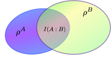
Figure 1: Schematic diagram for the quantum mutual information, $I(A:B)$, between two quantum states $\rho^{A}$ and $\rho^{B}$.

The von Neumann entropy, which is an extension of the Shannon entropy S48 to the quantum domain, can be estimated using quantum circuits and measurements. It is defined as the entropy of the density matrix associated with a quantum state, where the density matrix is a positive semi-definite matrix that represents the state. To estimate the von Neumann entropy, measurements can be performed on multiple copies of the quantum state and the outcomes of these measurements can be utilized. The most straightforward approach is to directly estimate the density matrix and calculate the entropy using its definition. However, estimating the von Neumann entropy can be challenging, particularly for large quantum systems, owing to the difficulty in accurately estimating the density matrix. Furthermore, the estimation accuracy is influenced by the number of measurements conducted and the quality of the quantum hardware employed. However, ongoing research is focused on developing more efficient and precise methods for estimating the von Neumann entropy.

Several methods have been employed to estimate von Neumann entropy, particularly those utilizing the quantum query model WZW22 ; GL19 ; SH21 . In the quantum query model, if the quantum circuit $U$ produces a quantum state $\rho$, it utilizes unitary gates such as $U$, $U^{\dagger}$, and C$U$ (controlled-$U$). However, the quantum circuit must be known to use the query model. The effectiveness of constructing a quantum query model for a given input state remains uncertain WZW22 , prompting us to explore the von Neumann entropy estimation without relying on the quantum query model. In the absence of a query model, our approach solely exploits identical copies of quantum states. Previous studies, such as Acharya et al. AISW20 employed $O(d^{2})$ copies of the quantum state $\rho$, where $d$ denotes the dimension, whereas Wang et al. WZW22 used $O\left(\frac{1}{\varepsilon^{5}\lambda^{2}}\right)$ copies of $\rho$, where $\lambda$ represents the lower bound on all nonzero eigenvalues. To the best of our knowledge, no existing algorithm provides a high-accuracy estimation of the von Neumann entropy by using only $O(\text{poly}(r))$ copies of $\rho$ with rank $r$.

II.2 Mutual Information Neural Estimator

The mutual information neural estimator (MINE) BBR+18 is a method for estimating the mutual information of two random variables by using neural networks. This approach involves selecting functions $T_{\theta}:X\times Y\rightarrow\mathbb{R}$ that are parameterized by neural networks with the parameter $\theta\in\Theta$. Considering $n$ samples, we define the empirical joint and product probability distributions as $p_{XY}^{(n)}$ and $p_{X}^{(n)}\times p_{Y}^{(n)}$, respectively. The MINE strategy is given by:

$$\widehat{I(X:Y)_{n}}=\sup_{\theta\in\Theta}\mathbb{E}_{p_{XY}}\left[T_{\theta}\right]-\log\left(\mathbb{E}_{p_{X}\times p_{Y}}\left[e^{T_{\theta}}\right]\right),$$ (2)

where ${\mathbb{E}}$ is the expected value. Additionally, the Donsker-Varadhan representation is defined as follows: For any probability distribution functions $p$ and $q$,

$$D_{KL}(p||q)=\sup_{T:\Omega\rightarrow\mathbb{R}}\mathbb{E}_{p}[T]-\log\left(\mathbb{E}_{q}\left[e^{T}\right]\right),$$ (3)

where we take the supremum over all the functions $T$.

Using the Donsker-Varadhan representation DV76 , it can be proven that $I\left(X:Y\right)\geq\widehat{I\left(X:Y\right)_{n}}$ and MINE are strongly consistent, meaning that there exists a positive integer $N$ and a choice of neural network parameters $\theta\in\Theta$ such that for all $n\geq N$, $\left|I(X:Y)-\widehat{I(X:Y)_{n}}\right|\leq\varepsilon$. By applying a gradient descent method on the neural network $T_{\theta}$ to maximize $\mathbb{E}_{p_{XY}}[T_{\theta}]-\log\left(\mathbb{E}_{p_{X}\times p_{Y}}\left[e^{T_{\theta}}\right]\right)$, we can obtain $\widehat{I(X:Y)_{n}}$ and estimate the mutual information $I(X:Y)$.

The MINE technique has found applications in various areas of artificial intelligence, such as feature selection, representation learning, and unsupervised learning, using information-theoretic methods. Compared to previous approaches, it provides more accurate and robust estimates of mutual information, leading to significant advancements in the field of artificial intelligence (AI). It is important to recognize that MINE is a relatively new and rapidly evolving field, with ongoing research focused on enhancing and broadening its capabilities. Nonetheless, the MINE technique is widely regarded as a valuable tool in AI and information theory, offering a powerful and flexible approach for estimating the mutual information between variables.

II.3 Parametrized Quantum Circuits

Parameterized quantum circuits (PQCs) BLSF19 are quantum circuits that incorporate adjustable parameters, typically represented as real numbers. These parameters can be fine-tuned to control the behavior of the quantum circuit, thereby providing increased flexibility and optimization potential. Parameterized quantum circuits have extensive applications in quantum machine learning and optimization algorithms, enabling computations that are challenging or even infeasible using classical methods. The key concept is to employ a parameterized quantum circuit as a feature extractor or waveform generator, followed by classical optimization algorithms that iteratively adjust the circuit parameters to minimize the objective function.

By manipulating circuit parameters, one can efficiently learn and represent quantum systems in a compact and adaptable manner. In quantum optimization, parameterized quantum circuits play a crucial role in global minimum search. By encoding the objective function into circuit parameters, quantum effects such as quantum parallelism and quantum tunneling can be harnessed to explore the search space more effectively than classical optimization algorithms. The objective function can be represented as a measurement outcome of the quantum circuit. The quantum circuit can harness superposition and entanglement to explore the search space more effectively than classical optimization algorithms.

One of the core techniques used in quantum optimization procedures for parameterized quantum circuits is the parameter shift rule MNKF18 . The parameter shift rule is a powerful tool in quantum machine learning that enables efficient computation of gradients with respect to the parameters of a quantum circuit.

The fundamental concept behind the parameter shift rule is to employ a quantum circuit with adjustable parameters to perform the measurements. By utilizing the measurement outcome, it is possible to estimate the gradient of a cost function with respect to the circuit parameters. This rule capitalizes on the notion that small variations in the parameters of a quantum circuit can be used to calculate the derivative of the cost function pertaining to these parameters.

The underlying principle involves the preparation of two identical copies of a quantum state, each with slightly different parameter values. By comparing these two quantum states, it was possible to estimate the gradient. More importantly, this method allows the calculation of gradients in a single pass through a quantum circuit, obviating the need for additional measurements. By using multiple samples via measurement, the gradient can be estimated.

If a parameterized quantum circuit is represented as a sequence of unitary gates, it is denoted as

$$U(x;\theta):=\left(\prod_{i=1}^{N}U_{i}(\theta_{i})\right)U_{0}(x).$$

The output of the circuit can then be observed using an observable $\hat{O}$ and the measurement outcome becomes a quantum circuit function. The quantum circuit function is expressed in simplified form as $f(x;\theta_{i})=\langle\psi_{i}|U_{i}^{\dagger}(\theta_{i})\hat{O}_{i+1}U_{i}(\theta_{i})|\psi_{i}\rangle$ for each $i$. The gradient of the quantum circuit function can then be calculated using the parameter shift rule, as follows:

$$\nabla_{\theta_{i}}f(x;\theta_{i})=c\left(\langle\psi_{i}|U_{i}^{\dagger}(\theta_{i}+s)\hat{O}_{i+1}U_{i}(\theta_{i}+s)|\psi_{i}\rangle-\langle\psi_{i}|U_{i}^{\dagger}(\theta_{i}-s)\hat{O}_{i+1}U_{i}(\theta_{i}-s)|\psi_{i}\rangle\right).$$ (4)

The parameter shift rule has been successfully employed in various quantum machine learning algorithms, including quantum neural networks BBF+20 ; BLSF19 and quantum support vector machines RML14 ; HCT+19 , for optimization and training purposes. It is regarded as a valuable tool for developing efficient quantum machine learning algorithms, as it enables the efficient computation of gradients in quantum systems, which is often a challenging task. It is important to note that the parameter shift rule is an approximation, and its accuracy depends on factors such as the choice of parameters, cost function, and the specific quantum circuit. Nevertheless, it has proven to be a useful and efficient technique in the emerging field of quantum machine learning, and our ongoing research focuses on enhancing and expanding its potential capabilities.

III Quantum Donsker-Varadhan Representation

The quantum Donsker-Varadhan representation is a mathematical framework that enables quantum neural networks to estimate the von Neumann entropy. It is a quantum counterpart of the original Donsker-Varadhan representation, with the distinction that QDVR focuses solely on the quantum entropy rather than on the relative entropy. QDVR can be considered as a modified version of the Gibbs variational principle H68 , which restricts the domain to density matrices.

As mentioned previously, MINE BBR+18 exploits the original Donsker-Varadhan representation to estimate classical mutual information using a (classical) neural network. In the context of estimating mutual quantum information, it is natural to consider a quantum version of the Donsker-Varadhan representation. Notably, we need only estimate the components of von Neumann entropy $S(\rho_{A})$, $S(\rho_{B})$, and $S(\rho_{AB})$ to determine the quantum mutual information $I(A:B)$. A variational formula for von Neumann entropy exists as follows:

Theorem 1 (Gibbs Variational Principle H68 ).

Let $f:H^{d\times d}\rightarrow\mathbb{R}$ be a function defined on $d$-dimensional Hermitian matrices $T$ and $\rho$ be a density matrix. Then we have

$$f(T)=-\mbox{$\textnormal{Tr}$}(\rho T)+\log\left(\mbox{$\textnormal{Tr}$}(e^{T})\right).$$ (5)

Thus, for $d$-dimensional Hermitian matrices $T$, the von Neumann entropy is given by:

$$S(\rho)=\inf_{T}f(T),$$ (6)

where the infimum is taken over all Hermitian $T$.

Our objective is to determine the Hermitian matrix $T$ that maximizes $f(T)$. We parameterize $T$ by using $t_{i}\in\mathbb{R}$ and $|\psi_{i}\rangle\in\mathbb{C}^{d}$. We can express $T=\sum_{i=1}^{r}t_{i}|\psi_{i}\rangle\langle\psi_{i}|$, which gives us $f(T)=-\sum_{i=1}^{d}t_{i}\langle\psi_{i}|\rho|\psi_{i}\rangle+\log\left(\sum_{i=1}^{d}e^{t_{i}}\right)$. To compute $f(T)$, we must measure the quantum state $\rho$ using the basis $\{|\psi_{i}\rangle\}_{i=1}^{d}$. Achieving this with an error smaller than $\varepsilon$ requires $O(\frac{\sigma^{2}}{\varepsilon^{2}})$ samples of $\rho$, where $\sigma:=\text{Var}(\{t_{i}\})$. However, the number of required samples of $\rho$ can become substantial because of the broad domain of $T$, which encompasses all Hermitian matrices. Therefore, reducing the size of this domain is imperative.

Lemma 2.

For all Hermitian matrices $T$, the function $f$ holds that

$$f(T)=f(T+cI)$$ (7)

for a constant $c$.

Proof.

For any $T\in H^{d\times d}$, we have

$$f(T+cI) =-\text{Tr}(\rho(T+cI))+\log\left(\text{Tr}(e^{T+cI})\right)$$

$$=-\text{Tr}(\rho T)-c\text{Tr}(\rho)+\log\left(e^{c}\text{Tr}(e^{T})\right)$$

$$=-\text{Tr}(\rho T)-\log\left(\text{Tr}(e^{T})\right)$$

$$=f(T).$$

Thus, $f(T)=f(T+cI)$ for a constant $c$. ∎

Proposition 1 (Domain Reduction).

Let $f:H^{d\times d}\rightarrow\mathbb{R}$ be a function defined on $d$-dimensional Hermitian matrices and let $\rho$ be a density matrix. Then,

$$S(\rho)=\inf_{T}f(T)$$ (8)

for $d$-dimensional ‘positive’ Hermitian matrices $T$.

Proof.

For any Hermitian matrix $T\in H^{d\times d}$, let $c=\max_{|\psi_{i}\rangle\in\mathbb{C}^{d}}(-\langle\psi_{i}|T|\psi_{i}\rangle)$. From Lemma 2, there exists a positive Hermitian matrix $T_{0}=T+cI$ such that $f(T)=f(T_{0})$. Therefore, we can reduce the domain of $T$ to a positive Hermitian matrix. ∎

Now, we only need to search for the space of the positive Hermitian matrices to find the optimal $T$. The computational complexity of copying $\rho$ to calculate $f(T)$ depends on $T$. To reduce this complexity, we need to specify and limit the trace of $T$.

Lemma 3.

A positive Hermitian matrix $T_{0}$ with rank $r$ exists that satisfies $\mbox{$\textnormal{Tr}$}(T_{0})\leq 2rn+r\log\left(\frac{1}{\varepsilon}\right)$ such that

$$\left|S(\rho)-f(T_{0})\right|<\varepsilon,$$ (9)

where $\rho$ is an $r$-rank density matrix.

Proof.

See the details of the proof in Appendix VII.1. ∎

Proposition 2 (Quantum Donsker-Varadhan Representation).

Let $f:H^{d\times d}\rightarrow\mathbb{R}$ be a function defined on $d$-dimensional Hermitian matrices, and let $\rho$ be an $r$-rank density matrix.

$$g(T)=-\mbox{$\textnormal{Tr}$}\left(c\rho T\right)+\log\left(\mbox{$\textnormal{Tr}$}(e^{cT})\right),$$ (10)

where $c\geq 2rn+r\log\left(\frac{1}{\varepsilon}\right)$. Then,

$$\left|S(\rho)-\inf(g(T))\right|<\varepsilon$$ (11)

for any $d$-dimensional $r$-rank density matrix $T$.

Proof.

By using Lemma 2 and Lemma 3, there exists an $r$-rank positive Hermitian matrix $T_{0}$ with $\text{Tr}(T_{0})=c$ such that $|S(\rho)-f(T_{0})|<\varepsilon$. Thus, $T_{1}=\frac{T_{0}}{c}$ is an $r$-rank density matrix, and $|S(\rho)-g(T_{1})|<\varepsilon$. From Theorem 1, $S(\rho)\leq g(T)$ for all density matrices $T$. Therefore, $\left|S(\rho)-\inf(g(T))\right|\leq\left|S(\rho)-g(T_{1})\right|<\varepsilon$. This completes the proof. ∎

According to the quantum Donsker-Varadhan representation in Proposition 2, we only need to search within the space of the density matrices. By calculating $g(T)$ with an error of $\varepsilon$, the complexity of copying $\rho$ is $O(\frac{c^{2}}{\varepsilon^{2}})$. Next, we plan to determine the optimal density matrix $T$ that minimizes $g(T)$. In the next section, we will use quantum neural networks to determine the optimal $T$.

IV Von Neumann Entropy Estimation with Quantum Neural Networks

We now explain the estimation of von Neumann entropy using quantum neural networks, specifically focusing on parameterized quantum circuits as an example. Our approach is inspired by the work of Liu et al. LMZW21 , who utilized variational autoregressive networks and quantum circuits to address problems in quantum statistical mechanics. To achieve this, specific values are assigned to the variables in $T$ by defining $t$ as a set of real numbers, $\{t_{i}|t_{i}\in\mathbb{R}\}$ and $|\psi_{i}\rangle$ as complex vectors in $\mathbb{C}^{d}$. Additionally, let us assume that the rank of $\rho$ is denoted by $r$, and we define $T=\sum^{r}_{i=1}t_{i}|\psi_{i}\rangle\langle\psi_{i}|$.

Consequently, the function $g(T)$ becomes $g(T)=-c\sum^{r}_{i=1}t_{i}\langle\psi_{i}|\rho|\psi_{i}\rangle+\log\left(d-r+\sum^{r}_{i=1}e^{ct_{i}}\right)$. We can introduce a unitary operator $U$ that transforms $|\psi_{i}\rangle$ into $|i\rangle$, and represent this unitary operator using a set of parameters $\theta$ as $U(\theta)$ as follows:

$$g(T)=-c\sum^{r}_{i=1}t_{i}\langle i|U(\theta)\rho U^{\dagger}(\theta)|i\rangle+\log\left(d-r+\sum^{r}_{i=1}e^{ct_{i}}\right).$$ (12)

By considering $U(\theta)$ as a quantum neural network and $\rho$ as its input, we can obtain the network output by computing $U(\theta)\rho U^{\dagger}(\theta)$. To accurately calculate $g(T)$ with an error rate less than $\varepsilon$, it is necessary to measure the output of the quantum neural network $O\left(\frac{\text{Var}({ct_{i}})^{2}}{\varepsilon^{2}}\right)=O\left(\frac{c^{2}}{\varepsilon^{2}}\right)$ times.

Our objective was to optimize the parameters to determine the infimum of $g(T)$. For example, let us consider a parameterized quantum circuit BLSF19 with Pauli gates as a quantum neural network $U(\theta)=\prod^{k}_{i=1}U(\theta_{i})$, where $U(\theta_{i})=e^{-i\frac{\theta_{i}}{2}P_{i}}$. By applying the parameter shift rule MNKF18 , we observe that

$$\nabla_{\theta}g(t,\theta)=\frac{1}{2}\left[g\left(t,\theta+\frac{\pi}{2}\right)-g\left(t,\theta-\frac{\pi}{2}\right)\right],$$ (13)

and

$$\frac{\partial g(t,\theta)}{\partial t_{i}}=-c\langle i|U(\theta)\rho U^{\dagger}(\theta)|i\rangle+\frac{ce^{ct_{i}}}{d-r+\sum^{r}_{i=1}e^{ct_{i}}}.$$ (14)

To satisfy the conditions $t_{i}\geq 0$ and $\sum^{r}_{i=1}t_{i}=1$, we choose $t_{i}=\left(\prod^{i-1}_{j=1}\sin^{2}\varphi_{j}\right)\left(\cos^{2}\varphi_{i}\right)$. We can apply gradient descent to $\varphi_{j}$ and $\theta_{i}$ to optimize the quantum circuit. To calculate the gradient, we require $O\left(\frac{c^{2}}{\varepsilon^{2}}\times\left(\text{\# of parameters in QNN}\right)\right)$ copies of $\rho$. Therefore, to obtain $\inf\left(g\left(T\right)\right)$ and estimate $S\left(\rho\right)$ with an error of less than $\varepsilon$, we require

$$O \left(\frac{c^{2}}{\varepsilon^{2}}\times\left(\text{\# of parameters in QNN}\right)\times\left(\text{\# of trainings in QNN}\right)\right)$$

$$=O\left(\frac{r^{2}}{\varepsilon^{2}}\left(n^{2}+\log^{2}\left(\frac{1}{\varepsilon}\right)\right)n_{\text{params}}n_{\text{train}}\right)$$ (15)

copies of $\rho$.

Analytic gradient measurements in convex loss functions require $O(\frac{n^{3}}{\varepsilon^{2}})$ copies of $\rho$ to converge to a solution with $O(\varepsilon)$ close to the optimum HN21 . In general, situations that involve parameterized quantum circuits may have nonconvex loss functions, but many algorithms still utilize parameterized quantum circuits and achieve quantum speedups. We anticipate that quantum speedup can be achieved by employing parameterized quantum circuits with analytic gradient measurements in QMINE and estimating the von Neumann entropy using $O(\text{poly}(r))$ copies of $\rho$. In future research, we will investigate the relationships between $n_{\text{train}}$ and $n_{\text{params}}$, and the performance of this approach. The key point is to transform the quantum mutual information estimation problem into a quantum neural network problem.

V Numerical Simulations

We demonstrated the performance of QMINE in estimating the quantum mutual information of random density matrices through numerical simulations of a quantum circuit. Our goal is to show that QMINE can estimate quantum mutual information with low error. We also analyze the rank and trainable parameters, and conducted simulations to support the results on QDVR.

V.1 Rank Analysis

Based on QDVR, we establish that if the rank of the density matrix $\rho$ is $r$, then setting the rank of the parameter matrix $T$ to $r$ is sufficient. Thus, we aim to determine the optimal $T$ that estimates the von Neumann entropy. To investigate the effect of rank, we experimented with the rank of $T$ by letting $r=\text{rank}(\rho)$ and $k=\text{rank}(T)$. In this analysis, we simulate the scenario with $N=5,D=30,r=8$, and $c\leq 80$, where $N$ is the number of qubits, $D$ is the circuit depth, $r$ is the rank of the density matrix, $c$ is calculated using QDVR (details are provided in Appendix VII.2). Figure 2 shows that when $k\geq r$, the result of QMINE converges to the correct value, whereas when $k<r$, it converges at a high error rate. This phenomenon has also been observed in other cases. These results support the QDVR’s claim that the rank of the optimal solution $T$ is $r$. Because convergence is faster when $k=r$ than when $k>r$, it is best to use QMINE with $k=r$.

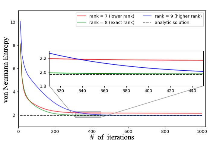
Figure 2: We compare the performance of different approaches. The green curve represents QMINE with the exact rank, which exhibited the best performance. It converges rapidly with low error. However, the red curve represents QMINE with a lower rank, which converges with a high error. Finally, the blue curve represents QMINE with a higher rank, which converges with low error but at a slower pace.

V.2 Number of Trainable Parameters on Quantum Circuit Analysis

We analyzed the performance of QMINE by varying the depth of the quantum circuit. In our simulations, we used $N=5$, $D=30$, $r=k=8$, and $c\leq 80$. The experimental results confirmed that as the depth of the circuit and the number of parameters increased, the estimation accuracy of QMINE improved. Fig. 3 illustrates the results, showing that a circuit depth of 20 achieved the best performance. It converged rapidly with a lower error compared to a depth of 30, which converged at a slower rate despite having a similar error. These findings emphasize the importance of choosing an appropriate circuit depth (i.e., number of parameters) in QMINE. The copy complexity is determined by the number of parameters ($n_{\text{params}}$) and the number of training iterations ($n_{\text{train}}$). Therefore, when applying QMINE in various situations, it is crucial to select the correct circuit depth. We plan to investigate this aspect in future studies.

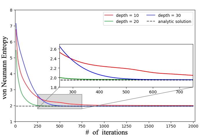
Figure 3: The green line in the graph, representing a circuit depth of 20 with 400 parameters, exhibits the best performance. It converges quickly with a low error-rate. However, the red line, representing a depth of 10 with 200 parameters, converges with a high error-rate. The blue line, corresponding to a depth of 30 with 600 parameters, achieves a low error but it takes a longer-time to converge.

V.3 Estimating Quantum Mutual Information

We estimated the quantum mutual information of a random density matrix using simulations with $N=4$ qubits. For each tested random density matrix, we achieved error rates ranging from $0.1\%$ to $1\%$. Additional details can be found in Appendix VII.2.

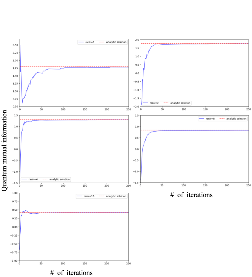
Figure 4: Estimation result of the quantum mutual information of a random density matrix.

VI Conclusions

We have addressed the quantum Donsker-Varadhan representation, which is a mathematical framework for estimating von Neumann entropy. The QDVR allows us to find the optimal $T$ by searching only within the density matrices, resulting in low copy complexity for calculations. By optimizing the quantum neural network using QDVR and the parameter shift rule, we can estimate von Neumann entropy and subsequently estimate the quantum mutual information. The number of copies of $\rho$ required is approximately $O\left(\frac{r^{2}}{\varepsilon^{2}}\left(n^{2}+\log^{2}\left(\frac{1}{\varepsilon}\right)\right)n_{\text{params}}\cdot n_{\text{train}}\right)$.

Through the numerical simulations, we demonstrated that the quantum mutual information neural estimation (QMINE) performs well, and it aligns with the results of quantum Donsker-Varadhan representation. The rank analysis supported the results of QDVR, whereas the circuit depth analysis emphasized the importance of selecting an appropriate circuit depth. In addition, we estimated the quantum mutual information and achieved a low error rate. The key finding of this study is the conversion of the quantum mutual information and von Neumann entropy estimation problem into a quantum neural network problem. In future, we suggest investigating the specifics of $n_{\text{params}}$ and $n_{\text{train}}$ pertaining to the quantum neural network problem. This will be explored in future studies.

Data availability

Our manuscript has no associated data.

Conflict of Interest

The authors have no conflicts to disclose.

VII Appendix

VII.1 Proof of Lemma 3

Here, we provide an explicit proof of Lemma 3 and details of the numerical simulation results.

For given $\rho=\sum^{r}_{i=1}p_{i}|\psi_{i}\rangle\!\langle\psi_{i}|$, let us define $T_{0}=\sum^{r}_{i=1}t_{i}|\psi_{i}\rangle\!\langle\psi_{i}|$ with $t_{i}=\begin{cases}\log(\frac{p_{i}}{k}),&{\textnormal{if}}\;\;p_{i}\geq k;\\ 0,&{\textnormal{if}}\;\;p_{i}<k\end{cases}$ and $k=\frac{\varepsilon}{d^{2}}$. Then, the bound on the value of $\left|S\left(\rho\right)-f\left(T_{0}\right)\right|$ can be derived as:

$$\left|S\left(\rho\right)-f\left(T_{0}\right)\right| =\left|S\left(\rho\right)+\mbox{$\textnormal{Tr}$}\left(\rho T_{0}\right)-\log\left(\mbox{$\textnormal{Tr}$}(e^{T_{0}})\right)\right|$$

$$=\left|\sum^{r}_{i=1}p_{i}\log\left(\frac{1}{p_{i}}\right)+\sum_{p_{i}\geq k}p_{i}\log\left(\frac{p_{i}}{k}\right)-\log\left(\sum_{p_{i}<k}1+\sum_{p_{i}\geq k}\frac{p_{i}}{k}\right)\right|$$

$$=\left|\sum_{p_{i}<k}p_{i}\log\left(\frac{1}{p_{i}}\right)+\sum_{p_{i}\geq k}p_{i}\log\left(\frac{1}{k}\right)-\log\left(\sum_{p_{i}<k}1+\sum_{p_{i}\geq k}\frac{p_{i}}{k}\right)\right|$$

$$=\left|\sum_{p_{i}<k}p_{i}\log\left(\frac{1}{p_{i}}\right)+\sum_{p_{i}\geq k}p_{i}\log\left(\frac{1}{k}\right)-\log\left(\frac{1}{k}\right)+\log\left(\frac{1}{k}\right)-\log\left(\sum_{p_{i}<k}1+\sum_{p_{i}\geq k}\frac{p_{i}}{k}\right)\right|$$

$$=\left|\sum_{p_{i}<k}p_{i}\log\left(\frac{k}{p_{i}}\right)-\log\left(\sum_{p_{i}<k}k+\sum_{p_{i}\geq k}p_{i}\right)\right|$$

$$=\left|\sum_{p_{i}<k}p_{i}\log\left(\frac{1}{p_{i}}\right)+\sum_{p_{i}<k}p_{i}\log\left(\frac{1}{k}\right)+\log\left(1+\sum_{p_{i}<k}\left(k-p_{i}\right)\right)\right|$$

$$\leq 2dk\log\left(\frac{1}{k}\right)+dk=\frac{2\varepsilon^{2}\left(2\log d+\log\left(\frac{1}{\varepsilon}\right)\right)}{d}+\frac{\varepsilon}{d}$$

$$<\varepsilon.$$

That is, $\left|S(\rho)-f(T_{0})\right|<\varepsilon$. Finally, $\mbox{$\textnormal{Tr}$}\left(T_{0}\right)$ is estimated as

$$\mbox{$\textnormal{Tr}$}\left(T_{0}\right) =\sum_{p_{i}\geq k}\log\left(\frac{p_{i}}{k}\right)\leq\sum_{p_{i}\geq k}\log\left(\frac{1}{k}\right)$$

$$\leq r\log\left(\frac{1}{k}\right)=2r\log d+r\log\left(\frac{1}{\varepsilon}\right)$$

$$=2rn+r\log\left(\frac{1}{\varepsilon}\right).$$

This implies that there exists a positive Hermitian matrix $T_{0}$ such that $\mbox{$\textnormal{Tr}$}(T_{0})=O(rn+r\log\left(\frac{1}{\varepsilon}\right))$ and $\left|S\left(\rho\right)-f\left(T_{0}\right)\right|<\varepsilon$. $\square$

VII.2 Details on Numerical Simulations

To support our observations, we explain the details of the numerical simulations for estimating the quantum mutual information, which can be expressed as the sum of von Neumann entropies as follows:

$$I\left(A:B\right) =S(\rho^{A})+S(\rho^{B})-S(\rho^{AB})$$

$$=S\left(\rho^{A}\otimes\rho^{B}\right)-S(\rho^{AB}).$$

To obtain quantum mutual information, we adopted an alternative and simple strategy. By exploiting QMINE (suggested in Sec.  IV), we directly estimate $S(\rho^{A}\otimes\rho^{B})$ and $S(\rho^{AB})$. That is, we address $S(\rho^{A}\otimes\rho^{B})$ rather than estimating $S(\rho^{A})$ or $S(\rho^{B})$. This method reduces the number of resource copies required for simulations.

We used four-qubit for this simulation and the results of our experiment are summarized in Table 1. To show that QMINE can estimate the quantum mutual information for various density matrices, we present the results of the estimation, where the rank of $\rho_{AB}$ is different.

Rank	QMI	Estimation results	Error-rate (%)
1	1.8048002	1.7946120	$0.565$
2	1.7631968	1.7493981	$0.783$
4	1.3031208	1.2902124	$0.991$
8	0.8440226	0.8376048	$0.760$
16	0.4172888	0.4163618	$0.222$

Table 1: Estimations of quantum mutual information using the QMINE method

References

- (1) G. Jaeger, “Quantum Information: An Overview,” Springer-Verlag, New York (2007).
- (2) M. A. Nielsen and I. L. Chuang, “Quantum Computation and Quantum Information,” Cambridge University Press (2000).
- (3) M. M. Wilde, “Quantum Information Theory,” Cambridge University Press (2013).
- (4) C. H. Bennett and P. W. Shor, “Quantum Channel Capacities,” Scienc 303, 1784 (2004).
- (5) A. S. Holevo, “Quantum channel capacities,” Quantum Electron. 50, 440 (2020).
- (6) J. Biamonte, P. Wittek, N. Pancotti, P. Rebentrost, N. Wiebe, and S. Lloyd, “Quantum machine learning,” Nature 549, 195 (2017).
- (7) G. Carleo, I. Cirac, K. Cranmer, L. Daudet, M. Schuld, N. Tishby, L. Vogt-Maranto, and L. Zdeborová, “Machine learning and the physical sciences,” Rev. Mod. Phys. 91, 045002 (2019).
- (8) I. Bengtsson and K. Życzkowski, “Geometry of quantum states: an introduction to quantum entanglement,” Cambridge University Press (2017).
- (9) R. O’Donnell and J. Wright, “Efficient quantum tomography,” Proceeding of the 48th Annual ACM Symposium on Theory of Computing, pp. 899–912 (2016).
- (10) M. B. Hastings, I. González, A. B. Kallin, and R. G. Melko, “Measuring Renyi Entanglement Entropy in Quantum Monte Carlo Simulations,” Phys. Rev. Lett. 104, 157201 (2010).
- (11) P. Calabrese, J. Cardy, and B. Doyon, “Entanglement entropy in extended quantum systems,” J. Phys. A: Math. Theor. 42, 500301 (2009).
- (12) T. Gur, M.-H. Hsieh, and S. Subramanian, “Sublinear quantum algorithms for estimating von Neumann entropy,” arXiv:2111.11139.
- (13) J. Acharya, I. Issa, N. V. Shende, and A. B. Wagner, “Estimating Quantum Entropy,” IEEE Journal on Selected Areas in Information Theory 1, 454 (2020).
- (14) K. C. Tan and T. Volkoff, “Variational quantum algorithms to estimate rank, quantum entropies, fidelity, and Fisher information via purity minimization,” Phys. Rev. Res. 3, 033251 (2021).
- (15) Y. Wang, B. Zhao, and X. Wang, “Quantum algorithms for estimating quantum entropies,” arXiv:2203.02386.
- (16) Q. Wang, J. Guan, J. Liu, Z. Zhang, and M. Ying, “New Quantum Algorithms for Computing Quantum Entropies and Distances,” arXiv:2203.13522.
- (17) A. Gilyén, and T. Li, “Distributional property testing in a quantum world,” arXiv:1902.00814.
- (18) S. Subramanian and M.-H. Hsieh, “Quantum algorithm for estimating -Renyi entropies of quantum states,” Phys. Rev. A 104, 022428 (2021).
- (19) J. von Neumann, “Mathematische grundlagen der quantenmechanik,” Springer-Verlag (1996).
- (20) K. Beer, D. Bondarenko, T. Farrelly, T. J. Osborne, R. Salzmann, D. Scheiermann, and R. Wolf, “Training deep quantum neural networks,” Nat. Commun. 11, 808 (2020).
- (21) K. H. Wan, O. Dahlsten, H. Kristjánsson, R. Gardner, and M. S. Kim, “Quantum generalisation of feedforward neural networks,” npj Quantum Inf. 3, 36 (2017).
- (22) M. Benedetti, E. Lloyd, S. Sack, and M. Fiorentini, “Parameterized quantum circuits as machine learning models,” Quantum Sci. Technol. 4, 043001 (2019).
- (23) J. R. McClean, S. Boixo, V. N. Smelyanskiy, R. Babbush, and H. Neven, “Barren plateaus in quantum neural network training landscapes,” Nat. Commun. 9, 4812 (2018).
- (24) Z. Goldfeld, D. Patel, S. Sreekumar, and M. M. Wilde, “Quantum Neural Estimation of Entropies,” arXiv:2307.01171.
- (25) C. E. Shannon, “A mathematical theory of communication,” Bell Syst. Tech. J. 27, 379 & 623 (1948).
- (26) M. I. Belghazi, A. Baratin, S. Rajeswar, S. Ozair, Y. Bengio, A. Courville, and R. D. Hjelm, “MINE: Mutual Information Neural Estimation,” arXiv:1801.04062.
- (27) M. D. Donsker, and S. R. S. Varadhan, “Asymptotic evaluation of certain Markov process expectations for large time—III,” Commun. Pure & App. Math. 29, 389 (1976).
- (28) K. Mitarai, M. Negoro, M. Kitagawa, and K. Fujii, “Quantum circuit learning,” Phys. Rev. A 98, 032309 (2018).
- (29) P. Rebentrost, M. Mohseni, and S. Lloyd, “Quantum Support Vector Machine for Big Data Classification,” Phys. Rev. Lett. 113, 130503 (2014).
- (30) V. Havlíček, A. D. Córcoles, K. Temme, A. W. Harrow, A. Kandala, J. M. Chow, and J. M. Gambetta, “Supervised learning with quantum-enhanced feature spaces,” Nature 567, 209 (2019).
- (31) A. Huber, “Variational Principles in Quantum Statistical Mechanics,” Mathematical Methods in Solid State and Superfluid Theory: Scottish Universities? Summer School, pp. 364–392 (1968).
- (32) J.-G. Liu, L. Mao, P, Zhang, and L. Wang, “Solving quantum statistical mechanics with variational autoregressive networks and quantum circuits,” Mach. Learn.: Sci. Technol. 2, 025011 (2021).
- (33) A. W. Harrow and J. C. Napp, “Low-Depth Gradient Measurements Can Improve Convergence in Variational Hybrid Quantum-Classical Algorithms,” Phys. Rev. Lett. 126, 140502 (2021).