A class of non linear adaptive time-frequency transforms

Abstract

This paper introduces a couple of new time-frequency transforms, designed to adapt their scale to specific features of the analyzed function. Such an adaptation is implemented via so-called focus functions, which control the window scale as a function of the time variable, or the frequency variable. In this respect, these transforms are non-linear, which makes the analysis more complex than usual.

Under appropriate assumptions, some norm control can be obtained for both transforms in $\textit{L}^{2}(\mathbb{R})$ spaces, which extend the classical continuous frame norm control and guarantees well-definedness on $\textit{L}^{2}$. Given the non-linearity of the transforms, the existence of inverse transforms is not guaranteed anymore, and is an open question. However, the results of this paper represent a first step towards a more general theory.

Besides mathematical results, some elementary examples of time and frequency focus functions are provided, which can serve as staring point for concrete applications.

1 Introduction

1.1 Context and purpose

Time-frequency transforms and generalisations (wavelets and others) have long been used in various theoretical and applied domains. Besides quadratic transforms (Wigner distributions and generalizations), linear transforms such as the Gabor/STFT [1, 2] and wavelet transforms [3, 1, 4, 5] generally enjoy simple and useful invertibility properties, and therefore allow describing functions and signals as linear combination of building blocks, called time-frequency atoms. The time (and frequency/scale) resolution of the latter is given by the construction rule: constant time and frequency resolution for Gabor/STFT, generated by translations and modulations, and constant relative frequency resolution for wavelets, generated by translations and rescalings. See also [6, 7, 8] for alternative constructions that implement other scaling rules. Variants were also considered in specific applied domains, such as the Stockwell transform [9] in geophysics, which is very close to the constant $Q$ transform [10, 11] we consider below, and the continuous wavelet transform.

In several application domains, in particular audio signal processing, it has been shown that adapting the scale of time-frequency atoms to the content of the signal can provide more efficient signal descriptions. The window size tunes the time-frequency resolution of the analysis. The latter is constrained by the uncertainty principle, which can be given various quantitative formulations (see [12, 13] and references therein), and which basically states that precision in time domain is possible at the price of precision loss in frequency domain, and vice versa. The problem of tuning time-frequency resolution as a function of time or frequency has been addressed by various authors, in various contexts, mostly with pre-defined dependence. As a motivation, even though there is no complete consensus on psycho-physical aspects of human perception, it is known to involve several non-linear effects [14], and it has been claimed that this non-linearity allows going beyond time-frequency uncertainty in terms of localisation [15]. Such strategy has been successfully implemented in some advanced audio coders such as AAC (see [16] for a short account), which can switch dynamically between short and long local cosine windows. Another possible motivation can be hyper-resolution (separation of close locally harmonic components in signals). However, the adaptation is often driven by prior heuristic computations, and the inversion of the corresponding transforms (if any) results from ad hoc adaptations. To our knowledge, the non-linear problem where the time-frequency resolution is adapted to the analysed function, has not been considered from the mathematical point of view so far.

The goal of the present paper is to introduce and study such adaptive time-frequency transforms, able to adapt their time-frequency resolution to the analysed function. This is done here by introducing a focus function $f\mapsto\sigma_{f}$ which adapts the shape (size, bandwidth etc…) of the analyse window to specific properties of the analysed signal $f$. Stepping away from fixed time-frequency resolution complexifies significantly the analysis. The purpose of this article is to introduce properly the non linear transforms, prove that this class of transform are well defined on $L^{2}$ and provide explicit, signal-dependent, lower and upper bounds for their norm (which depends on the choice of focus function). We first introduce in Section 2 a generalisation of a constant Q transform studied in [11, 17], and prove an isometry result, using notations and ideas that will be useful for the rest of the paper. Section 3 introduces our first adaptive transform $M^{\nu}$ that associates with a signal $f$ a focus function $\sigma_{f}^{\nu}:\,\omega\mapsto\sigma^{\nu}_{f}(\omega)$ defined in the frequency domain. We then prove in Theorem 3.8 the well-definedness of $M^{\nu}$ as a map from $L^{2}(\mathbb{R})$ into $L^{2}(\mathbb{R}^{2})$ and obtain a norm control of the form $c_{f}\|f\|\leq\|M^{\nu}f\|\leq C_{f}\|f\|$, with explicit constants $c_{f},C_{f}$, under suitable assumptions on the focus function $\sigma_{f}^{\nu}$. In section 4 we introduce a time-focused transform $M^{\tau}$ which associates with a signal $f$ a focus function of $\sigma_{f}^{\tau}:\,t\mapsto\sigma^{\tau}_{f}(t)$ defined in the time domain. We prove similar norm control and $L^{2}$ well-definedness results, using a suitable non linear kernel. We also give in Sections 3 and 4 explicit examples of focus functions which may be of interest in applications, and illustrate their behaviour on toy examples in the Appendix. Section 5 is devoted to conclusions and perspectives.

1.2 Notations

We first introduce or recall a few notations. We will often use the notation $C([a,b],X)$ for the space of continuous functions from $\mathbb{R}$ into $X$, supported in $[a,b]$. More generally, given $A\subset\mathbb{R}^{\mathbb{R}}$ we denote by $A_{c}$ the subspace of functions in $A$ with compact support, and by $A_{0}$ the subspace of functions in $A$ which vanish at infinity. We define $A+c:=\{f+c,f\in A\}$ for $c\in\mathbb{R}$ and $A^{+}$ denotes the subspace of non-negative valued functions on $A$.

Given an open interval $I$ in $\mathbb{R}$, $C^{n}(I)$ stands for the space of function which are $n$ times derivable on $I$, and $C^{\infty}(I)=\cap_{n\geqslant 0}C^{n}(I)$, furthermore we denote by $C_{p}(I)$ the space of piecewise continuous functions on $I$. Finally, we denote by $\mathcal{E}$ the space of step functions, and by $\mathcal{E}([a,b])$ the space of step function with support included in $[a,b]$.

We recall that $L^{p}(\mathbb{R}^{d})$ is the set of $p-$integrable functions (quotiented out by the classical equivalence relationship), for $p>1$. The shorter notation $L^{p}$ refers to $L^{p}(\mathbb{R})$. When no measure is specified it means that we are working with the Lebesgue measure, otherwise we write $L^{p}(\mathbb{R}^{d},d\mu)$ with $d\mu$ a regular enough measure on $\mathbb{R}^{d}$. For functions of several variables, we use the notation $\mathbb{R}^{d}_{t}$ to specify that $t\in\mathbb{R}^{d}$. The notation $L^{p}(\mathbb{R}^{d}_{t},L^{q}(\mathbb{R}^{l}_{x}))$ stands for functions $f$ for which the above mixed norm is finite

$$\|f\|_{L^{p}_{t}L^{q}_{x}}:=\left(\int_{\mathbb{R}^{d}}\left(\int_{\mathbb{R}^{l}}|f(x,t)|^{q}dx\right)^{p/q}dt\right)^{1/p}\ .$$ (1)

When there is no risk of confusion, $d$ and $l$ will be omitted and we will simply write $L^{p}_{t}L^{q}_{x}$. More generally, for given two normed functional spaces $A(\mathbb{R}^{d})$ and $B(\mathbb{R}^{l})$ then $A_{t}B_{x}=A(\mathbb{R}^{d}_{t},B(\mathbb{R}^{l}_{x}))$ is the set of function $f:\mathbb{R}^{d}\times\mathbb{R}^{l}\rightarrow\mathbb{C}$ for which the above mixed norm is finite,

$$\|f\|_{A_{t}B_{x}}:=\|\|f(x,t)\|_{B_{x}}\|_{A_{t}}\ .$$ (2)

Given $f\in L^{p}$ its Fourier transform is either written $\mathcal{F}(f)$ or $\hat{f}$ and defined by the following convention if $f\in L^{1}$,

$$\mathcal{F}(f)(\omega):=\int_{\mathbb{R}^{d}}f(x)e^{-2i\pi x\cdot\omega}dx\ ,$$ (3)

for any $\omega\in\mathbb{R}^{d}$ for which the right hand side is well-defined.

2 A generalised constant Q transform

Before introducing frequency and time focus, we first introduce a slight generalisation of a standard constant Q transform (CQT for short). We consider the general framework of continuous time-frequency/time-scale transforms, the prototype of which is given by the Short Time Fourier Transform (STFT, see [2] for a detailed exposition) and the continuous wavelet transforms [3]. The constant $Q$ transform was introduced in a discrete context [10] and revisited more recently [11, 17], we give below a slightly more general version adapted to the continuous setting.

The purpose of this section is to introduce the first tools used for our non linear transform but also some methods and computations that will be directly applied in section 3.

2.1 Definition of the time-frequency atoms

The time-frequency atoms are built from a reference waveform $h$, which will be assumed continuous and compactly supported in the Fourier domain. From this, time-frequency atoms $h_{t,\textit{u}}$ are generated as

$$\forall x,t,\textit{u}\in\mathbb{R}\ ,\quad\ h_{t,u}(x):=\sqrt{\gamma(u)}e^{2i\pi\gamma(u)x}h(\gamma(u)x-t)\ ,$$ (4)

where u is a frequency index, mapped to a frequency variable by the function $\gamma$.

Remark 1.

To make sense from a physical point of view, the variable $t$ has to be seen as a dimensionless time variable, therefore $\gamma(\textit{u})$ has to be understood as a dimensionless frequency.

The frequency function $\gamma$ is assumed to be a positive, increasing $C^{1}$ diffeomorphism, such that $\lim_{u\to-\infty}\gamma(u)=0$ and $\lim_{u\to+\infty}\gamma(u)=+\infty$. In [17, 11], $\gamma$ was given an exponential form, we consider here a slightly more general such scale function.

For technical reasons, the reference waveform $h$ will also be supposed to be symmetric with respect to $-1$ in the Fourier domain, which suggests to write $h$ as

$$\forall x\in\mathbb{R},\ h(x)=h_{r}(x)e^{-2i\pi x}\ ,$$ (5)

where $h_{r}$ can be chosen real valued. An example of such a reference waveform could be a shifted version of frequency domain Hann, or raised cosine

$$\hat{h}(\xi)=\mathds{1}_{[-3,1]}(\xi)\cos^{2}(\tfrac{\pi}{2}\xi)\ ,$$ (6)

whose form in the time domain reads

$$h(x)=\frac{\sin(4\pi x)}{4\pi x(1-4x^{2})}e^{-2i\pi x}\ .$$ (7)

We can now introduce the generalised Viennese constant Q transform [11]. Let $f\in C_{c}(\mathbb{R})$, then we define the transform through inner products with time-frequency atoms,

$$\forall t,\textit{u}\in\mathbb{R},\ Lf(t,\textit{u}):=\langle f,h_{t,\textit{u}}\rangle_{L^{2}_{x}}\ .$$ (8)

The normalisation by $\sqrt{\gamma}$ ensures norm conservation, i.e. $\|h_{t,\textit{u}}\|_{L^{2}_{x}}=\|h\|_{L^{2}_{x}}$ for any $t,\textit{u}\in\mathbb{R}$. However such normalisation leads us to work in the modified $L^{2}(d\mu)$ space where the measure is defined by $d\mu(t,\textit{u}):=\tfrac{\gamma^{\prime}(\textit{u})}{\gamma(\textit{u})}d\textit{u}dt$. The pointwise definition on $L^{2}$ is guaranteed by the fact that by assumption, $h$ is continuous and compactly supported in the frequency domain, therefore $h\in L^{2}$.

In order to determine the first norm control we need to compute the Fourier transform of the atoms and for the sake of simplicity let us introduce the auxiliary function $\beta_{\xi}$ defined by

$$\beta_{\xi}(\textit{u}):=\gamma(\textit{u})^{-1}\xi-1\ .$$ (9)

Now the Fourier transform of the atoms reads

$$\mathcal{F}(h_{t,\textit{u}})(\xi)=\sqrt{\gamma(\textit{u})}\int_{\mathbb{R}}e^{-2i\pi x(\xi-\gamma(\textit{u}))}h(\gamma(\textit{u})x-t)dx\ .$$ (10)

Using the change of variable $y=\gamma(\textit{u})x-t$, we obtain

$$\mathcal{F}(h_{t,\textit{u}})(\xi) =\frac{1}{\sqrt{\gamma(\textit{u})}}\int_{\mathbb{R}}e^{-2i\pi\beta_{\xi}(\textit{u})(y+t)}h(y)dy$$ (11)

$$=\frac{1}{\sqrt{\gamma(\textit{u})}}e^{-2i\pi\beta_{\xi}(\textit{u})t}\hat{h}(\beta_{\xi}(\textit{u}))\ .$$ (12)

2.2 Admissibility condition and norm equality

Given these definitions and notations, we can now state the first results, namely the well-definedness of the operator from $L^{2}(\mathbb{R},dx)$ into $L^{2}(\mathbb{R}^{2},d\mu)$ and an explicit expression for the norm of the transform. Such results are summed up in the following Proposition.

Proposition 1.

Let $\gamma$ be a $C^{1}$ diffeomorphism such that $\lim_{\textit{u}\to-\infty}\gamma(\textit{u})=0$ and $\lim_{\textit{u}\to+\infty}\gamma(\textit{u})=+\infty$, and $h$ being a continuous and compactly supported in the Fourier domain. Assume that $h$ satisfies the following admissibility conditions

$$0<c_{h}:=\int_{-1}^{+\infty}\frac{|\hat{h}(y)|^{2}}{y+1}dy=\int_{-\infty}^{-1}\frac{|\hat{h}(y)|^{2}}{-y-1}dy<\infty\ .$$ (13)

Then for any $f\in L^{2}(\mathbb{R},dx)$ we have

$$\|Lf\|^{2}_{L^{2}(\mathbb{R}^{2},d\mu)}=c_{h}\|f\|_{L^{2}(dx)}^{2}\ .$$ (14)

Notice that the right hand side equality in the above admissibility condition can be satisfied whenever $\hat{h}$ is symmetric with respect to -1, which is a simple and easy to fulfil condition.

Proof 2.1.

Let $f\in C_{c}^{\infty}$. Using Fubini’s lemma we obtain

$$\|Lf\|_{L^{2}(d\mu)}^{2}=\int\bar{\hat{f}}(\xi)\hat{f}(\xi^{\prime})\hat{h}(\beta_{\xi}(\textit{u}))\bar{\hat{h}}(\beta_{\xi^{\prime}}(\textit{u}))\frac{1}{\gamma(\textit{u})}e^{-2i\pi(\gamma(\textit{u})^{-1}(\xi-\xi^{\prime}))t}d\xi d\xi^{\prime}\frac{\gamma^{\prime}(\textit{u})}{\gamma(\textit{u})}d\textit{u}dt\ .$$

By inverse Fourier transform this gives us that

$$\|Lf\|_{L^{2}(d\mu)}^{2} =\int_{\mathbb{R}}|\hat{f}(\xi)|^{2}\int_{\mathbb{R}}\frac{\gamma^{\prime}(\textit{u})}{\gamma(\textit{u})}|\hat{h}(\beta_{\xi}(\textit{u}))|^{2}d\textit{u}d\xi$$

which concludes the first step of the proof. For the second part, let us set $y:=\beta_{\xi}(\textit{u})$. Hence $\textit{u}=\gamma^{-1}(\frac{\xi}{y+1})$ and $d\textit{u}=-\frac{\gamma^{2}(\textit{u})}{\xi\gamma^{\prime}(\textit{u})}dy$. Since the limits $\lim_{\textit{u}\to\pm\infty}\beta_{\xi}(\textit{u})$ depend on the sign of $\xi$ we have to split the integral in two terms.

$$\|Lf\|_{L^{2}}^{2} =\int_{\mathbb{R}}|\hat{f}(\xi)|^{2}\int_{\mathbb{R}}\frac{\gamma^{\prime}(\textit{u})}{\gamma(\textit{u})}|\hat{h}(\beta_{\xi}(\textit{u}))|^{2}d\textit{u}d\xi$$

$$=\underset{=:(a)}{\underbrace{\int_{\mathbb{R}^{+}}|\hat{f}(\xi)|^{2}\int_{\mathbb{R}}\frac{\gamma^{\prime}(\textit{u})}{\gamma(\textit{u})}|\hat{h}(\beta_{\xi}(\textit{u}))|^{2}d\textit{u}d\xi}}+\underset{=:(b)}{\underbrace{\int_{\mathbb{R}^{-}}|\hat{f}(\xi)|^{2}\int_{\mathbb{R}}\frac{\gamma^{\prime}(\textit{u})}{\gamma(\textit{u})}|\hat{h}(\beta_{\xi}(\textit{u}))|^{2}d\textit{u}d\xi}}\ .$$

For the first term $(a)$ we have $y(\textit{u})=\frac{\xi}{\gamma(\textit{u})}-1$ so $\lim_{u\to-\infty}y(u)=+\infty$ and $\lim_{u\to+\infty}y(u)=-1$ thus by the same change of variables as above we have

$$(a) =\int_{\mathbb{R}^{+}}|\hat{f}(\xi)|^{2}\int_{-1}^{+\infty}\frac{\gamma^{\prime}(\textit{u})}{\gamma^{\prime}(\textit{u})}\frac{\gamma^{2}(\textit{u})}{\xi\gamma(\textit{u})}|\hat{h}(y)|^{2}dy$$

$$=\int_{\mathbb{R}^{+}}|\hat{f}(\xi)|^{2}d\xi\int_{-1}^{+\infty}\frac{|\hat{h}(y)|^{2}}{y+1}dy=c_{h}\int_{\mathbb{R}^{+}}|\hat{f}(\xi)|^{2}d\xi\ .$$

The evaluation of the second term $(b)$ is similar but - due to the fact that $\lim_{u\to-\infty}y(u)=-\infty$ and $\lim_{u\to+\infty}=-1$ - we obtain at the end

$$(b)=\int_{\mathbb{R}^{-}}|\hat{f}(\xi)|^{2}d\xi\int_{-\infty}^{-1}\frac{-|\hat{h}(y)|^{2}}{y+1}dy=c_{h}\int_{\mathbb{R}^{-}}|\hat{f}(\xi)|^{2}d\xi\ .$$

This gives us after the change of variables $y^{\prime}:=-2-y$ and by condition (13),

$$(b)=\int_{\mathbb{R}^{-}}|\hat{f}(\xi)|^{2}d\xi\int_{-1}^{+\infty}\frac{|\hat{h}(y)|^{2}}{y+1}dy\ ,$$

which allows us to conclude by summing up the two terms and by density of $C_{c}^{\infty}$ in $L^{2}$.

One purpose of such result is to guarantee the existence of a left inverse operator thanks to the classical Hilbertian analysis result, which we quote here for the sake of completeness.

Proposition 1 (Proposition 2.17 from [18]).

Let $H,H^{\prime}$ be $\mathbb{K}-$Hilbert spaces and $T:H\rightarrow H^{\prime}$ and linear map. Then we have the existence of a left inverse if and only if $T$ is an isometry, furthermore such inverse is the conjugate map $T^{*}=\overline{T^{t}}$.

Following this idea we can compute the proper inverse operator which is given as follows. Such result is similar to the one we can find in the classical time frequency transforms.

Proposition 2 (Inversion formula).

The following inversion formula is true in $L^{2}$.

$$f=\frac{1}{c_{h}}\int Lf(t,\textit{u})h_{t,\textit{u}}\,d\mu(\textit{u},t)\ .$$ (15)

Remark 2.2.

1. The admissibility condition (13) is reminiscent of the continuous wavelet transform (CWT). Indeed, expressed in terms of $h_{r}$ defined in (5), $Lf$ is actually a CWT of $f$ with wavelet $h_{r}$ as defined in (5), combined with a frequency scaling $\gamma$ that may differ from the usual $\gamma(\textit{u})=2^{\textit{u}}$. The admissibility condition then becomes the usual wavelet admissibility condition on $h_{r}$.

2. Like the STFT and the continuous wavelet transform, alternative inversion formulas can be obtained by using different windows for the analysis and the synthesis, say $h$ as before and $w$. With the very same calculations as above, one obtains

   $$f=\frac{1}{c_{hw}}\int Lf(t,\textit{u})w_{t,\textit{u}}\,d\mu(t,\textit{u})\ ,$$

   with

   $$c_{hw}=\int_{-1}^{\infty}\frac{\overline{\hat{h}}(y)\hat{w}(y)}{y+1}dy=\int_{-\infty}^{-1}\frac{\overline{\hat{h}}(y)\hat{w}(y)}{-y-1}dy\ ,$$

   assuming $c_{hw}$ is nonzero and the corresponding integrals converge.

3 Time frequency transform with frequency focus

3.1 Definition of the transform

We now introduce the frequency focus effect, generated by the associated frequency focus function $\sigma^{\nu}$. The role of the focus function is to modify the shape of the analysis waveforms, in a way that depends on some local behaviour of the analysed signal $f$. Starting from the construction described in Section 2, the time-frequency atoms $h_{t,\textit{u}}$ are locally rescaled using a so called focus function $\sigma^{\nu}_{f}$, which depends on $f$. This yields new atoms that will be denoted by $h_{t,\textit{u},\sigma^{\nu}_{f}}$, $t$ denoting time and $u$ being the frequency scaling .

Assumptions

As in the previous section, $\gamma$ is assumed to be a positive, increasing $C^{1}$ diffeomorphism that maps $\mathbb{R}$ onto $\mathbb{R}_{+}$. The focus functions $\sigma^{\nu}_{f}$ of $f\in L^{2}(\mathbb{R})$ will be assumed to be at least piecewise continuous, larger than 1 and such that $\sigma_{f}^{\nu}-1$ is compactly supported. To sum up

$$\forall f\in L^{2}(\mathbb{R}),\ \sigma^{\nu}_{f}\in C_{p,c}^{+}(\mathbb{R})+1\ .$$ (16)

Atoms and transform

Given these notations, the Viennese constant-Q transform with frequency focus effect (or frequency-Marseillan transform) $M^{\nu}$ can be defined for $f\in C_{c}$ by

$$\forall t,\textit{u}\in\mathbb{R}\ ,\quad\ M^{\nu}f(t,\textit{u}):=\langle f,h_{t,\textit{u},\sigma^{\nu}_{f}}\rangle_{L^{2}_{x}}\ ,$$ (17)

the time-frequency atoms being defined by

$$\forall x,t,\textit{u}\in\mathbb{R}\,,\quad h_{t,\textit{u},\sigma_{f}^{\nu}}(x):=\sigma_{f}^{\nu}(\textit{u})\sqrt{\gamma(\textit{u})}e^{2i\pi\gamma(\textit{u})x}h((\gamma(\textit{u})x-t)\sigma_{f}^{\nu}(\textit{u}))\ .$$ (18)

Remark 3.3.

In order to keep constant $L^{2}$ norm for the atoms, we should normalize them by $\sqrt{\sigma_{f}}$ instead of $\sigma_{f}$, however with such normalisation $d\mu$ will not be a measure anymore which goes beyond the borders of our study.

The main purpose of the section is to establish that $M^{\nu}$ can be extended to a well defined map from $L^{2}(\mathbb{R},dx)\rightarrow L^{2}(\mathbb{R}^{2},d\mu)$ satisfying a norm control similar to a frame bound control. The pointwise definition of $M^{\nu}f(t,\textit{u})$ on $L^{2}$ is still guaranteed by the fact that $h\in L^{2}$. Regarding the definition from $L^{2}$ into $L^{2}(\mathbb{R}^{2},d\mu)$ we can raise that $M^{\nu}$ is well defined from $C_{c}$ into $L^{2}$ and then extend the control by the use of the Fatou’s lemma.

By computations similar as the previous section, we obtain the following Fourier transform of the atoms,

$$\mathcal{F}(h_{t,\textit{u},\sigma^{\nu}(\textit{u})})(\xi)=\frac{1}{\sqrt{\gamma(\textit{u})}}\hat{h}\left(\beta_{\xi}(\textit{u})/\sigma^{\nu}(\textit{u})\right)e^{-2i\pi\beta_{\xi}(\textit{u})t}\ .$$ (19)

Sometimes, if there are no ambiguities we will write $h_{t,\textit{u},f}$ instead of $h_{t,\textit{u},\sigma_{f}}$ and $h_{t,\textit{u},n}$ instead of $h_{t,\textit{u},\sigma_{f_{n}}}$ for a certain sequence $(f_{n})_{n}$.

3.2 Example and ideas of the frequency focus function

Defining and studying specific frequency focus functions is not a main goal of this paper. We can however provide a toy example that could be of interest in some specific situations.

Example 3.4 (Resolving close frequencies).

Imagine a function $f$ of interest contains several harmonic components (i.e. sine waves) with more or less close frequencies. When consecutive frequencies are too close, a wideband window will not be able to separate them, which would suggest to increase the frequency precision in the neighborhood of these frequencies. A prototypical choice for frequency focus function in such a context could be

$$\sigma_{f}^{\nu}(\textit{u})=1+\frac{\|V_{g}f(\cdot,\textit{u})\|_{L^{1}(dt)}}{\|V_{g}f(\cdot,\textit{u})\|_{L^{2}(dt)}}\,\varphi(\textit{u})\ ,$$ (20)

where $\varphi$ is compactly supported in some interval $[-\textit{u}_{0},\textit{u}_{0}]$ for some cutoff frequency $\textit{u}_{0}$ ($\varphi$ can be a multiple of the indicator function of that interval, or the hearing threshold in psycho-physical applications), and $V_{g}$ is the ordinary STFT, with gaussian window [2].
The ratio of $L^{1}$ to $L^{2}$ norms is known as a a measure of spread, or diversity (it takes small values when the corresponding function is more concentrated, and is closely related to a specific Renyi entropy, see [13]). When $f$ contains several sine waves in the neighbourhood of u, which are not separated by the gaussian window, some beats appear in the function $t\mapsto V_{g}f(t,\textit{u})$, which yields smaller $L^{1}/L^{2}$ norm values, and therefore small values for $\sigma_{f}^{\nu}(\textit{u})$.

Illustrations with a suitably post-processed version of this choice, on a toy signal example, is provided in Appendix A.1.

3.3 Kernel and norm relationship

To prove the main result we first derive a norm relationship involving a certain non-negative valued kernel $K_{\sigma}$, so that the study of the norm of $M^{\nu}f$ will be determined by the norm $\|K_{\sigma}\|_{\infty}$.

Proposition 3.

Let us assume that $h$ satisfies the same admissibility condition as in Proposition 1. Then we have

$$\|M^{\nu}f\|_{L^{2}(d\mu)}^{2}=\int_{\mathbb{R}}|\hat{f}(\xi)|^{2}K_{\sigma_{f}^{\nu}}(\xi)d\xi\ ,$$ (21)

where the kernel $K_{\sigma_{f}^{\nu}}(\xi)$ is defined by

$$K_{\sigma_{f}^{\nu}}(\xi):=\int_{-1}^{+\infty}\left|\hat{h}\left(\frac{y}{\sigma_{f}^{\nu}\circ\gamma^{-1}(|\frac{\xi}{y+1}|)}\right)\right|^{2}\frac{dy}{|y+1|}\ .$$ (22)

Remark 3.5.

Since $\sigma\circ\gamma^{-1}(|\frac{\xi}{y+1}|)=1$ for $y$ big enough or close enough to $-1$, thanks to the admissiblity condition on $h$ (see equation 13) the convergence of $K_{\sigma}$ is guaranteed.

Proof 3.6.

Introducing $\sigma(\textit{u})$ in the proof of Proposition 1 gives us

$$\|M^{\nu}f\|^{2}_{L^{2}} =\int\bar{\hat{f}}(\xi)\hat{f}(\xi^{\prime})\frac{1}{\gamma(\textit{u})}\hat{h}(\beta_{\xi}(\textit{u})/\sigma_{f}^{\nu}(\textit{u}))\bar{\hat{h}}(\beta_{\xi^{\prime}}(\textit{u})/\sigma_{f}^{\nu}(\textit{u}))e^{-2i\pi\gamma(\textit{u})^{-1}(\xi-\xi^{\prime})t}d\xi d\xi^{\prime}d\mu(\textit{u},t)$$

$$=\int|\hat{f}(\xi)|^{2}\frac{\gamma^{\prime}(\textit{u})}{\gamma(\textit{u})^{2}}|\hat{h}(\beta_{\xi}(\textit{u})/\sigma_{f}^{\nu}(\textit{u})|^{2}d\xi d\textit{u}$$

$$=(1)+(2)\ ,$$

where

$$(1) :=\int_{0}^{+\infty}|\hat{f}(\xi)|^{2}\int_{-\infty}^{+\infty}\frac{\gamma^{\prime}(\textit{u})}{\gamma(\textit{u})^{2}}|\hat{h}(\beta_{\xi}(\textit{u})/\sigma_{f}^{\nu}(\textit{u})|^{2}d\textit{u}d\xi,$$

$$(2) :=\int_{-\infty}^{0}|\hat{f}(\xi)|^{2}\int_{-\infty}^{+\infty}\frac{\gamma^{\prime}(\textit{u})}{\gamma(\textit{u})^{2}}|\hat{h}(\beta_{\xi}(\textit{u})/\sigma_{f}^{\nu}(\textit{u})|^{2}d\textit{u}d\xi\ .$$

Using the same change of variable $y=\beta_{\xi}(\textit{u})$ in both cases and taking care of the signs we get (1) and in (2) the sign of $\xi/(y+1)$ is still non negative as $\xi\leqslant 0$ and $y\leqslant-1$ so we obtain

$$(1) =\int_{0}^{+\infty}|\hat{f}(\xi)|^{2}\int_{-1}^{+\infty}\left|\hat{h}\left(\frac{y}{\sigma_{f}^{\nu}\circ\gamma^{-1}(\frac{\xi}{y+1})}\right)\right|^{2}\frac{dy}{y+1}d\xi,$$

$$(2) =-\int_{-\infty}^{0}|\hat{f}(\xi)|^{2}\int_{-\infty}^{-1}\left|\hat{h}\left(\frac{y}{\sigma_{f}^{\nu}\circ\gamma^{-1}(\frac{\xi}{y+1})}\right)\right|^{2}\frac{dy}{y+1}d\xi$$

$$=\int_{-\infty}^{0}|\hat{f}(\xi)|^{2}\int_{-\infty}^{-1}\left|\hat{h}\left(\frac{y}{\sigma_{f}^{\nu}\circ\gamma^{-1}(|\frac{\xi}{y+1}|)}\right)\right|^{2}\frac{dy}{|y+1|}d\xi.$$

Using a symmetry argument similar to the proof of proposition (1), and summing both terms we obtain the expected formula.

Remark 3.7.

If $\sigma$ is fixed and independent of $f$, the time-frequency atoms $h_{t,\omega,\sigma(\omega)}$ form a continuous frame of $L^{2}(\mathbb{R})$ in the terminology of [7, 19]. We will see that in the general case, the assumptions made on $\sigma$ allow one to stay in a tractable situation.

From now, the goal is to obtain upper and lower bounds for the kernel $K_{\sigma}$.

3.4 Main result : the $L^{2}$ norm control

The main result of this section is the following theorem 3.8 which is a generalisation to non linear transform with adaptive window of the classical frame control.

Theorem 3.8.

Let $f\in L^{2}(\mathbb{R})$ and $\sigma^{\nu}_{f}\in C_{c}^{+}(\mathbb{R})\cap C_{p}+1$ with support included in $[a,b]$, $a\leqslant b$. Then we have

$$c_{a,b}\|f\|_{L^{2}(dx)}\leqslant\|M^{\nu}f\|_{L^{2}(d\mu)}\leqslant C_{a,b}\|f\|_{L^{2}(dx)},$$ (23)

where the constants $c_{a,b}$ and $C_{a,b}$ are given by

$$C_{a,b}^{2}:=\int_{-1}^{+\infty}|\hat{h}(y)|^{2}\frac{dy}{y+1}+\|\hat{h}\|_{\infty}^{2}\ln\left(\frac{\gamma(b)}{\gamma(a)}\right)<+\infty,$$ (24)

and

$$c_{a,b}^{2}:=\inf_{\xi_{0}\in\mathbb{R}}\{r^{-}(\xi_{0})+r^{+}(\xi_{0})\}>0,$$ (25)

with

$$r^{-}(\xi):=\int_{-1}^{-1+|\xi|/\gamma(b)}\frac{|\hat{h}(y)|^{2}}{y+1}dy\ ,\quad r^{+}(\xi):=\int_{-1+|\xi|/\gamma(a)}^{+\infty}\frac{|\hat{h}(y)|^{2}}{y+1}dy\ .$$ (26)

Remark 3.9.

We can raise that if $\sigma$ is fixed (i.e.  independent of $f$) then we obtain the classical bound control from linear time frequency operators since $c_{a,b}$ and $C_{a,b}$ only depend on $\sigma$ and not directly on $f$. More precisely they only depend on the support of $\sigma$.

Proof 3.10.

Even though $\sigma_{f}$ is supposed to be piecewise continuous, the idea of the proof is to control the sup norm of the kernel $K_{\kappa}$ when $\kappa\in\mathcal{E}_{c}^{+}+1$ with $\mathcal{E}$ the set of step functions and $\kappa$ close enough to $\sigma$. Everything will be defined correctly in the next section. The reason of such idea is because for step functions $\kappa$ the kernel $K_{\kappa}$ is easy to estimate. Thus by using the control for step functions and proving a continuity result of $K_{\kappa}$ for functions $\kappa\rightarrow\sigma$ we will be able to prove our control for continuous (pr piecewise continuous) focus functions $\sigma_{f}$.

3.5 Proof of the theorem 3.8 : approach by step functions

3.5.1 Decomposition lemma

We introduce the decomposition lemma 3.11 that is a key part of the study of the kernel onto step functions. Indeed it turns out that when $\kappa\in\mathcal{E}^{+}([a,b])+1$, then $K_{\kappa}$ can be expressed in quite a simple way which yields ’easy’ estimates depending only on the support $[a,b]$ and $h$.

Lemma 3.11 (Decomposition of the Kernel).

Let $\kappa(x):=1+\lambda\mathds{1}_{[a,b]}(x)$, $a<b$ and $\lambda\geqslant 0$, thus

$$\forall\xi\in\mathbb{R},\qquad K_{\kappa}(\xi)=\int_{[-1,+\infty)\backslash[\beta_{|\xi|}(b),\beta_{|\xi|}(a)]}\frac{|\hat{h}(y)|^{2}}{|y+1|}\,dy\ +\ \int_{\beta_{|\xi|}(b)}^{\beta_{|\xi|}(a)}\frac{|\hat{h}(\tfrac{y}{1+\lambda})|^{2}}{|y+1|}\,dy\ .$$ (27)

Proof 3.12.

If $\xi=0$ then the lemma is clearly true, so let us assume $\xi\not=0$. Now let us raise that $\sigma\circ\gamma^{-1}(\textit{u})=1+\mathds{1}_{[\gamma(a),\gamma(b)]}(\textit{u})$ thus $\sigma\circ\gamma^{-1}(|\tfrac{\xi}{y+1}|)=1+\mathds{1}_{[\gamma(a),\gamma(b)]}(|\tfrac{\xi}{y+1}|)$. In order to have $\sigma\circ\gamma^{-1}(|\tfrac{\xi}{y+1}|)=1+\lambda$ there are two possible situations : either $-1+\frac{\xi}{\gamma(b)}\leqslant y\leqslant-1+\frac{\xi}{\gamma(a)}$ (case (1)) or $-1-\frac{\xi}{\gamma(a)}\leqslant y\leqslant-1-\frac{\xi}{\gamma(b)}$ (case (2)). Since $y\geqslant-1$ only one case is possible at the time. When $\xi>0$ case (2) is not possible but (1) is, so we have the desired decomposition

$$K_{\kappa}(\xi)=\int_{[-1,+\infty)\backslash[\beta_{\xi}(b),\beta_{\xi}(a)]}\frac{|\hat{h}(y)|^{2}}{|y+1|}\,dy+\int_{\beta_{\xi}(b)}^{\beta_{\xi}(a)}\frac{|\hat{h}(\tfrac{y}{1+\lambda})|^{2}}{|y+1|}\,dy\ .$$ (28)

However if $\xi<0$ only case (2) is possible and thus the decomposition is

$$K_{\kappa}(\xi)=\int_{[-1,+\infty)\backslash[\beta_{-\xi}(b),\beta_{-\xi}(a)]}\frac{|\hat{h}(y)|^{2}}{|y+1|}\,dy+\int_{\beta_{-\xi}(b)}^{\beta_{-\xi}(a)}\frac{|\hat{h}(\tfrac{y}{1+\lambda})|^{2}}{|y+1|}\,dy\ .$$ (29)

Combining both decompositions yields the result.

Following the same ideas we can easily generalise the decomposition lemma to more complex step functions.

Lemma 3.13.

Lets $\kappa(x):=1+\sum_{i=0}^{n}\lambda_{i}\mathds{1}_{[a_{i},b_{i}]}(x)$ with $\lambda_{i}\geqslant 0$ and $a_{i}\leqslant b_{i}\leqslant a_{i+1}$. Then we have

$$\forall\xi\in\mathbb{R}\,,\quad\ K_{\kappa}(\xi)=\int_{[-1,+\infty)\backslash[\beta_{|\xi|}(b),\beta_{|\xi|}(a)]}\frac{|\hat{h}(y)|^{2}}{|y+1|}dy+\sum_{i=0}^{n}\int_{\beta_{|\xi|}(b_{i})}^{\beta_{|\xi|}(a_{i})}\frac{|\hat{h}(\tfrac{y}{1+\lambda_{i}})|^{2}}{|y+1|}dy\ .$$ (30)

Besides giving us an important decomposition of the integral it also gives us the symmetry properties of our object, and will then allow us to restrain to $\xi\geqslant 0$ all computations which involve this decomposition (as long as they are symmetric on $\xi$ on their others parts).

3.5.2 Upper bound control

Before introducing the general upper bound result we first prove a weaker result that concerns function of the form : $\kappa(\textit{u})=1+\lambda\mathds{1}_{[a,b]}(\textit{u})$.

Proposition 4.

Let $a<b$ and $\kappa(\textit{u})=1+\lambda\mathds{1}_{[a,b]}(\textit{u})$, then we have

$$\forall\xi,\ K_{\kappa}(\xi)\leqslant\int_{-1}^{+\infty}\frac{|\hat{h}(y)|^{2}}{|y+1|}dy+\|\hat{h}\|_{L^{\infty}}^{2}\ln\left(\frac{\gamma(b)}{\gamma(a)}\right).$$ (31)

Proof 3.14.

Using Lemma 3.11 we obtain for $\xi\geqslant 0$

$$K_{\kappa}(\xi) =\int_{[-1,+\infty)\backslash[-1+\frac{\xi}{\gamma(b)},-1+\frac{\xi}{\gamma(a)}]}\frac{|\hat{h}(y)|^{2}}{|y+1|}dy+\int_{-1+\frac{\xi}{\gamma(b)}}^{-1+\frac{\xi}{\gamma(a)}}\frac{|\hat{h}(\tfrac{y}{1+\lambda})|^{2}}{|y+1|}dy$$ (32)

$$\leqslant\int_{-1}^{+\infty}\frac{|\hat{h}(y)|^{2}}{|y+1|}dy+\|\hat{h}\|_{L^{\infty}}^{2}\int_{-1+\frac{\xi}{\gamma(b)}}^{-1+\frac{\xi}{\gamma(a)}}\frac{1}{|y+1|}dy$$ (33)

$$=\int_{-1}^{+\infty}\frac{|\hat{h}(y)|^{2}}{|y+1|}dy+\|\hat{h}\|_{L^{\infty}}^{2}\ln\left(\frac{\gamma(b)}{\gamma(a)}\right).$$ (34)

The same computation can be performed in the case $\xi<0$.

The norm $\|\hat{h}\|_{L^{\infty}}$ is easy to control since it is below $\|h\|_{L^{1}}$. What is interesting with this first result is the fact that the control is independent of $\lambda$. The result is easy to generalise, by splitting the integral into as many terms as there are subdivisions. This gives Proposition 5 below.

Proposition 5.

Let $(a_{i})_{0\leqslant i\leqslant n},(b_{i})_{0\leqslant i\leqslant n}$ such that $a_{i+1}>b_{i}$, $(\lambda_{i})_{0\leqslant i\leqslant n}\in(\mathbb{R}_{+}^{*})^{n+1}$ and $\sigma(x)=1+\sum_{i=0}^{n}\lambda_{i}\mathds{1}_{[a_{i},b_{i}]}(x)$ then

$$\forall\xi\in\mathbb{R},\ K_{\sigma}(\xi)\leqslant\int_{-1}^{+\infty}\frac{|\hat{h}(y)|^{2}}{|y+1|}dy+\|\hat{h}\|_{L^{\infty}}^{2}\sum_{i=0}^{n}\ln\left(\frac{\gamma(b_{i})}{\gamma(a_{i})}\right)\ .$$ (35)

A consequence of such control is that there exists a constant $C^{+}_{a,b}$ that depends on the window $h$ and on $a,b$ such that for any $\kappa\in\mathcal{E}^{+}([a,b])+1$ we have

$$\|K_{\kappa}\|_{\infty}\leqslant C_{a,b}^{2}:=\int_{-1}^{+\infty}\frac{|\hat{h}(y)|^{2}}{|y+1|}dy+\|\hat{h}\|_{L^{\infty}}^{2}\ln\left(\frac{\gamma(b)}{\gamma(a)}\right)\ .$$ (36)

Proof 3.15.

The proof is the same as the previous one except that Lemma 3.13 is used and the contribution of every sub-interval $[-1+\xi/\gamma(b_{i}),-1+\xi/\gamma(a_{i})]$ has to be controlled.

Even though it is not the best possible control, this bound is strong enough for our purpose in Theorem 3.8. A stronger control for a specific $\kappa$ could be the following one but since it depends too much on the values of $(a_{i}),(b_{i}),(\lambda_{i})$ we will not use it later.

Proposition 6.

Let $\kappa(x)=\sum_{i=0}^{n}\lambda_{i}\mathds{1}_{[a_{i},b_{i}]}(x)$ with $\lambda_{i}\geqslant 0$ and $a_{i+1}\geqslant b_{i}$, then

$$\forall\xi\in\mathbb{R},\quad|K_{\kappa}(\xi)|\leqslant\int_{-1}^{+\infty}\frac{|\hat{h}(y)|^{2}}{y+1}dy+\max_{0\leqslant i\leqslant n}\sup_{[B_{i}^{\xi},A_{i}^{\xi}]}\{|\hat{h}(y)|^{2}\}\sum_{j=0}^{n}\ln\left(\frac{\gamma(b_{j})}{\gamma(a_{j})}\right)\ ,$$ (37)

where $A_{i}^{\xi}=\frac{-1+\xi/\gamma(a_{i})}{1+\lambda_{i}},B_{i}^{\xi}=\frac{-1+\xi/\gamma(b_{i})}{1+\lambda_{i}}$.

Proof 3.16.

We use the same decomposition as previously, thus letting $0\leqslant i\leqslant n$ we have

$$\int_{-1+\xi/\gamma(b_{i})}^{-1+\xi/\gamma(a_{i})}\frac{|\hat{h}(\tfrac{y}{1+\lambda_{i}})|^{2}}{y+1}dy \leqslant\sup_{[B_{i}^{\xi},A_{i}^{\xi}]}\{|\hat{h}(y)|^{2}\}\ln\left(\frac{\gamma(b_{i})}{\gamma(a_{i})}\right)$$ (38)

and taking the max over $0\leqslant i\leqslant n$, summing the log and keeping the rest $\int|\hat{h}(y)|^{2}/(y+1)dy$ we obtain the desired result.

3.5.3 Lower bound control

The following result guarantees the existence of a positive lower bound that only depends on the support of the focus function.

Proposition 7.

Let $a<b\in\mathbb{R}$ and $\kappa\in\mathcal{E}([a,b],\mathbb{R}^{+})+1$, for any $\xi\in\mathbb{R}$ we define

$$r^{-}(\xi):=\int_{-1}^{-1+|\xi|/\gamma(b)}\frac{|\hat{h}(y)|^{2}}{y+1}dy$$ (39)

and

$$r^{+}(\xi):=\int_{-1+|\xi|/\gamma(a)}^{+\infty}\frac{|\hat{h}(y)|^{2}}{y+1}dy\ .$$ (40)

Then we have

$$\inf_{\xi}|K_{\kappa}(\xi)|\geqslant\inf_{\xi_{0}\in\mathbb{R}}\{r^{-}(\xi_{0})+r^{+}(\xi_{0})\}=:c_{a,b}^{2}\ .$$ (41)

Furthermore, under our hypothesis $c_{a,b}>0$.

Proof 3.17.

A separation trick similar to what was done in Lemma 3.11 gives us, for any $\xi\in\mathbb{R}$,

$$K_{\kappa}(\xi) =\int_{-1}^{-1+|\xi|/\gamma(b)}\frac{|\hat{h}(y)|^{2}}{y+1}dy$$

$$+\int_{-1+|\xi|/\gamma(b)}^{-1+|\xi|/\gamma(a)}\left|\hat{h}\left(\frac{y}{\kappa\circ\gamma^{-1}(|\frac{\xi}{y+1}|)}\right)\right|^{2}\frac{dy}{|y+1|}$$

$$+\int_{-1+|\xi|/\gamma(a)}^{+\infty}\frac{|\hat{h}(y)|^{2}}{y+1}dy.$$

Hence by taking the $\inf$ we obtain the expected control, furthermore by continuity of $r^{\pm}(\xi)$ and by positivity at every $\xi\in\mathbb{R}$ and at the limits at $\pm\infty$ of at least $r^{+}$ or $r^{-}$ we can conclude on the positivity of $c_{a,b}$.

3.5.4 Continuity and general norm control

We recall that a function $f:\mathbb{R}\rightarrow\mathbb{C}$ is uniformly continuous if

$$\forall\varepsilon>0,\,\exists\delta(\varepsilon)>0,\,\forall x,y\in\mathbb{R},\,|x-y|\leqslant\delta(\varepsilon)\Rightarrow|f(x)-f(y)|\leqslant\varepsilon\ .$$ (42)

Of course there is no uniqueness of $\delta(\varepsilon)$ but we can take anyone that satisfies equation (42). We can now state the continuity result that is the key point of the whole section.

Proposition 8 (Continuity of the Kernel).

Assume that $|\hat{h}|\in C_{0}(\mathbb{R})$, then $|\hat{h}|^{2}$ is uniformly continuous with constant $\delta(\varepsilon)>0$ for $\varepsilon>0$. And let $\sigma\in C([a,b])^{+}\cap C_{p}+1$. Then there exists $\xi_{0}(\varepsilon)>0$ such that for any $\kappa\in\mathcal{E}([a,b])+1$ satisfying $\kappa(x)\leqslant\sigma(x)$ and

$$\|\sigma-\kappa\|_{\infty}\leqslant\tilde{\delta}(\varepsilon):=\frac{\delta(\varepsilon)\gamma(a)}{\xi_{0}(\varepsilon)}\ ,$$ (43)

we have

$$\|K_{\sigma}-K_{\kappa}\|_{\infty}\leqslant\varepsilon\ln\left(\frac{\gamma(b)}{\gamma(a)}\right)\ .$$ (44)

Proof 3.18.

Let us first raise that for $\sigma\in C^{+}([a,b])+1$ and $\kappa\in\mathcal{E}^{+}([a,b])+1$ then we have for any $\xi\in\mathbb{R}$,

$$|K_{\sigma}(\xi)-K_{\kappa}(\xi)|=\left|\int_{-1+\frac{|\xi|}{\gamma(b)}}^{-1+\frac{|\xi|}{\gamma(a)}}\left|\hat{h}\left(\frac{y}{\sigma\circ\gamma^{-1}(\frac{\xi}{y+1})}\right)\right|^{2}-\left|\hat{h}\left(\frac{y}{\kappa\circ\gamma^{-1}(\frac{\xi}{y+1})}\right)\right|^{2}\frac{dy}{y+1}\right|\ .$$

Therefore, for a fixed $\xi$ we will be working on bounded intervals, which will be is important for the rest of the proof. The main idea is the following : consider the quantity $|K_{\kappa}(\xi)-K_{\sigma}(\xi)|$ in two cases. The first one will be for $\xi\geqslant\xi_{0}$ large enough such that the integrated quantity will be small because $\hat{h}$ tends to infinity at $\pm\infty$. The second case will be for $\kappa$ close enough with respect to $\varepsilon$ and $\xi_{0}$ so that the difference in the integral will be small enough.

Since $|\hat{h}|$ tends to $0$ at $\pm\infty$ we have the existence of $y_{0}(\varepsilon)$ such that for any $|y|\geqslant y_{0}$ the quantity $|\hat{h}(y)|^{2}\leqslant\varepsilon/2$. Hence there exist $\xi_{0}(\varepsilon)$ such that $\xi_{0}/\gamma(b)\geqslant 1$ and $\frac{\xi_{0}/\gamma(b)-1}{\|\sigma\|_{\infty}}\geqslant y_{0}(\varepsilon)$. Furthermore since for any $\xi\geqslant\xi_{0}$ and any $y\in[-1+\frac{\xi}{\gamma(b)},-1+\frac{\xi}{\gamma(a)}]$ we have

$$\frac{y}{\sigma\circ\gamma^{-1}(\frac{|\xi|}{y+1})}\geqslant\frac{\frac{|\xi|}{\gamma(b)}-1}{\|\sigma\|_{\infty}}\geqslant\frac{\frac{|\xi_{0}|}{\gamma(b)}-1}{\|\sigma\|_{\infty}}\geqslant y_{0}(\varepsilon)\ ,$$ (45)

then we have the following control

$$|K_{\sigma}(\xi)-K_{\kappa}(\xi)| \leqslant\varepsilon\int_{-1+\frac{|\xi|}{\gamma(b)}}^{-1+\frac{|\xi|}{\gamma(a)}}\frac{dy}{y+1}$$

$$\leqslant\varepsilon\ln\left(\frac{\gamma(b)}{\gamma(a)}\right)\ .$$

This concludes the first part of the proof. Now for such $\xi_{0}$ fixed lets take $\tilde{\delta}(\varepsilon):=\frac{\delta(\varepsilon)\gamma(a)}{\xi_{0}(\varepsilon)}$ and $\kappa$ satisfying the hypothesis of the proposition. Then for any $|\xi|\leqslant\xi_{0}$ and $y\in[-1+\frac{|\xi|}{\gamma(b)},-1+\frac{|\xi|}{\gamma(a)}]$ we have

$$\left|\frac{y}{\sigma\circ\gamma^{-1}(\frac{|\xi|}{y+1})}-\frac{y}{\kappa\circ\gamma^{-1}(\frac{|\xi|}{y+1})}\right| =|y|\frac{|\kappa\circ\gamma^{-1}(\frac{|\xi|}{y+1})-\sigma\circ\gamma^{-1}(\frac{|\xi|}{y+1})|}{\kappa\circ\gamma^{-1}(\frac{|\xi|}{y+1})\sigma\circ\gamma^{-1}(\frac{|\xi|}{y+1})}$$

$$\leqslant|y|\tfrac{\delta(\varepsilon)\gamma(a)}{\xi_{0}}$$

$$\leqslant\left|-1+\tfrac{|\xi|}{\gamma(a)}\right|\,\tfrac{\delta(\varepsilon)\gamma(a)}{\xi_{0}}$$

$$\leqslant\delta(\varepsilon).$$

Hence for $|\xi|\leqslant\xi_{0}$ (and the assumptions on $\kappa$ made in Proposition  8) we obtain by uniform continuity of $\hat{h}$,

$$|K_{\sigma}(\xi)-K_{\kappa}(\xi)|\leqslant\varepsilon\ln\left(\frac{\gamma(b)}{\gamma(a)}\right).$$

The $|\hat{h}|^{2}$ uniform continuity hypothesis is neither absurd nor a constraint. Indeed if $h$ is in $L^{1}$ then by Riemann-Lebesgue lemma and property of the Fourier transform we have that $\hat{h}\in C_{0}$ and so is $|\hat{h}|^{2}$. Having that leads to the uniform continuity of $|\hat{h}|^{2}$.

The following Lemma 3.19 results from the lower and upper bounds of the triangular inequality.

Lemma 3.19.

Let $\sigma\in C^{+}([a,b])+1$ and $\kappa\in\mathcal{E}^{+}([a,b])+1$, then for any $\xi\in\mathbb{R}$,

$$|K_{\kappa}(\xi)|-|K_{\sigma}(\xi)-K_{\kappa}(\xi)|\leqslant|K_{\sigma}(\xi)|\leqslant|K_{\sigma}(\xi)-K_{\kappa}(\xi)|+|K_{\kappa}(\xi)|.$$ (46)

Putting together Lemma 3.19, Proposition 8, Proposition 7 and Proposition 5 yields Theorem  3.8.

4 The non linear time focused operator

4.1 Atoms and time focused transform

Let us now introduce and study the second nonlinear transform of interest here, namely the time focused transform, which involves a focus function defined in the time domain. Even though the ideas behind the transform are the same as the ones developed for frequency focus, the definition and the method used to prove the needed results are completely different from the one used in Section 3.

Assumptions

One of the first differences with the frequency focused operator are the assumptions on the frequency function $\gamma$. In this section $\gamma$ is a $C^{1}$ symmetrical diffeomorphism satisfying $\lim_{t\to-\infty}\gamma(t)=-\infty$ and $\lim_{t\to+\infty}\gamma(t)=+\infty$. A prototypical $\gamma$ could be hyperbolic sinus shape like, i.e. very precise around $0$ (low frequencies) and less precise for high values (high frequencies).

We will assume the window $h$ to be continuous (at least piecewise) and with compact support of size $l\in\mathbb{R}^{+}_{*}$. An example of such window would be the Hamming window. About the focus function of $f$ - written $\sigma_{f}^{\tau}$ - we will assume it to be grater than $1$, continuous (at least piecewise) and only vanishing at infinity (not necessarily with compact support), i.e.

$$\forall f\in L^{2}(\mathbb{R}),\ \sigma^{\tau}_{f}\in C^{+}_{p,0}(\mathbb{R})+1.$$ (47)

In order to lighten the notations we will sometimes omit the subscript $\tau$ when there are no ambiguities.

Remark 4.20.

Whereas in the previous transforms $Lf$ and $M^{\nu}$ the second variable $u$ is a ’frequency index’, here $\omega$ is directly a frequency and the meaning of $\gamma$ is a bit different in this section. The function $\gamma$ is still homogeneous to a frequency, however it models a non linearity in the precision of the analysis along the frequency axis.

Atoms and transform definition

Given hypotheses we can define the time focused atoms .

$$\forall x,t,\omega\in\mathbb{R},\ h_{t,\omega,\sigma_{f}^{\tau}}(x):=\sqrt{\gamma^{\prime}(\omega)\sigma(t)}e^{2i\pi\gamma(\omega)x}h(\sigma_{f}^{\tau}(t)(x-t))\ ,$$ (48)

and the transform of a given signal $f\in L^{2}$ by

$$\forall t,\omega\in\mathbb{R},\ M^{\tau}f(t,\omega):=\langle f,h_{t,\omega,\sigma_{f}^{\tau}}\rangle_{L^{2}_{x}}.$$ (49)

The pointwise definition of the scalar product is guaranteed by the fact that $h(\sigma(t)(x-t))$ is a compactly supported function of $x$.

Sometimes, if there are no ambiguities we will write $h_{t,\omega,f}$ instead of $h_{t,\omega,\sigma_{f}}$ and $h_{t,\omega,n}$ instead of $h_{t,\omega,\sigma_{f_{n}}}$ for a certain sequence $(f_{n})_{n}$.

Density result

In order to justify as much as possible the validity of our further computations we will prove the following density result which state that if we take a $L^{2}$ function $f$ and a $C_{c}$ function $f_{\varepsilon}$ as close as possible in $L^{2}$ to $f$ then the norm of $M^{\tau}f$ will be controlled by the norm of $M^{\tau}f_{\varepsilon}$ which is finite thanks to basic integration rules.

Lemma 4.21.

Let $f\in L^{2}$ and $(f_{n})_{n}\in(C_{c})^{\mathbb{N}}$ be such that $f_{n}\rightarrow f$ in $L^{2}$ and $\sigma(f_{n})=:\sigma_{n}\rightarrow\sigma(f)$ in $L^{\infty}$ then

$$\forall\varepsilon>0,\exists N\in\mathbb{N},\forall n\geqslant N,\left|\|M^{\tau}f\|_{L^{2}}-\|M^{\tau}f_{n}\|_{L^{2}}\right|\leqslant\varepsilon\ .$$ (50)

Proof 4.22.

We have

$$\left|\|M^{\tau}f_{n}\|^{2}_{L^{2}}-\|M^{\tau}f\|^{2}_{L^{2}}\right| =\left|\iint_{\mathbb{R}^{2}}|\langle f_{n},h_{t,\omega,n}\rangle|^{2}d\omega dt-\iint_{\mathbb{R}^{2}}|\langle f,h_{t,\omega,f}\rangle|^{2}d\omega dt\right|$$

$$=\left|\int_{\mathbb{R}}A(t)dt+\int_{\mathbb{R}}B(t)dt\right|,$$

with

$$A(t) :=\int_{\mathbb{R}}\sigma_{f}(t)h^{2}(\sigma_{f}(t)(x-t))\left(|f_{n}(x)|^{2}-|f(x)|^{2}\right)dx\ .$$

Hence

$$\int_{\mathbb{R}}|A(t)|dt\leqslant\|\sigma_{f}\|_{\infty}\|h(\sigma_{f}(t)(x-t))\|_{L^{\infty}_{x,t}}\varepsilon\ .$$

Similarly

$$B(t):=\int_{\mathbb{R}}\sigma_{n}(t)|f_{n}(x)|^{2}\left(h^{2}(\sigma_{n}(t)(x-t))-h^{2}(\sigma_{f}(t)(x-t))\right)dx\ ,$$

thus

$$\int_{\mathbb{R}}|B(t)|dt\leqslant(\|\sigma_{f}\|_{\infty}+\varepsilon)(\|f\|_{L^{2}}+\varepsilon)^{2}2l\varepsilon\ .$$

The result alone does not allow us to extend directly the well-definedness from $C_{c}$ to $L^{2}$. However we will see that combined with the upper bound control proved in Proposition 10 it will allow us to conclude about the well-definedness of $M^{\tau}$ on $L^{2}$.

4.2 Example and ideas of the time focus function

Again, it is not the goal of the current paper to discuss in details explicit choices for the focus functions that would be relevant in specific applications. We only provide a simple and generic example that could be of interest (a more sophisticated alternative, developed in the context of audio compression, can be found in [20]).

Example 4.23 (Adaptation to transient events).

As already mentioned in the introduction, a fairly natural idea is to increase the time resolution of the analysis when the analysed signal has faster variations. This requires a heuristics to measure such speed of variations. As in Example 3.4, a ratio of suitably chosen norms can be used for that purpose. Using frequency content as a measure of speed of variations, one may consider the quantity

$$\sigma_{f}^{\tau}(t):=1+\sqrt{\frac{\int_{\mathbb{R}}|\omega|^{2n}|V_{g}f(t,\omega)|^{2}d\omega}{\int_{\mathbb{R}}|V_{g}f(t,\omega)|^{2}d\omega}}\varphi(t)\ ,$$ (51)

with $V_{g}f$ the STFT of $f$ with gaussian window $g(x):=e^{-x^{2}/2a^{2}}$ with variance $a^{2}$, and $\varphi$ an additional function, which can ensure constant support and appropriate normalisation. The rationale is to use the ratio to measure some frequency content of the signal around time $t$ (as an average frequency variable, weighted by the spectrogram at time $t$). The higher the average frequency, the larger the time focus, and smaller the adapted window. A toy example is given in Appendix A.2 that shows the ability of such functions to detect transient events in a signal and therefore adapt the scale of a window in the time focused transform.

4.3 Norm relationship and time kernel

Following the same ideas as in Section 3 we will determine an equality of the $L^{2}$ norm of $Mf$ and introduce a certain time dependent kernel. Beside being useful for the rest of the study the equality guarantees the well-definedness of the transform on $L^{2}$.

However one main difference with the frequency kernel is that we will be able to have an explicit expression or at least a way easier to manipulate expression of the kernel. The first result gives us the norm relationship in Fourier.

Proposition 9.

Using the previous definition, for $f\in C_{c}$ we have then

$$\|M^{\tau}f\|_{L^{2}}^{2}=\iint_{\mathbb{R}^{2}}\hat{f}(\xi)\bar{\hat{f}}(\xi^{\prime})K_{\sigma_{f}^{\tau}}(\xi-\xi^{\prime})d\xi d\xi^{\prime},$$ (52)

where the time kernel is

$$K_{\sigma_{f}^{\tau}}(u):=\iint_{\mathbb{R}^{2}}e^{-2i\pi ut}\bar{\hat{h}}(z)\hat{h}\left(z-\tfrac{u}{\sigma_{f}^{\tau}(t)}\right)\,dzdt\ .$$ (53)

Proof 4.24.

In order to make notations lighter we use $\sigma$ for $\sigma_{f}^{\tau}$. The computations are quite similar than the one used in the proofs of the frequency focus.

$$\|M^{\tau}f\|_{L^{2}}^{2} =\iint_{\mathbb{R}^{2}}|\langle\hat{f},\hat{h}_{t,\omega,\sigma}\rangle|^{2}dtd\omega$$

$$=\iiiint_{\mathbb{R}^{4}}\hat{f}(\xi)\bar{\hat{f}}(\xi^{\prime})\bar{\hat{h}}_{t,\omega,\sigma}(\xi)\hat{h}_{t,\omega,\sigma}(\xi^{\prime})d\xi d\xi^{\prime}dtd\omega$$

$$=\iint_{\mathbb{R}^{2}}\hat{f}(\xi)\bar{\hat{f}}(\xi^{\prime})\underset{=:K_{\sigma}(\xi,\xi^{\prime})}{\underbrace{\iint_{\mathbb{R}^{2}}\bar{\hat{h}}_{t,\omega,\sigma}(\xi)\hat{h}_{t,\omega,\sigma}(\xi^{\prime})dtd\omega}}d\xi d\xi^{\prime}$$

We have

$$K_{\sigma}(\xi,\xi^{\prime}):=\iint_{\mathbb{R}^{2}}\frac{\gamma^{\prime}(\omega)}{\sigma(t)}e^{-2i\pi(\xi-\xi^{\prime})t}\bar{\hat{h}}\left(\tfrac{\xi-\gamma(\omega)}{\sigma(t)}\right)\hat{h}\left(\tfrac{\xi^{\prime}-\gamma(\omega)}{\sigma(t)}\right)\,d\omega dt\ .$$

Hence, by setting $y(\omega)=-\frac{\gamma(\omega)}{\sigma(t)}$ we obtain

$$K_{\sigma}(\xi,\xi^{\prime}) =\iint_{\mathbb{R}^{2}}\bar{\hat{h}}\left(\tfrac{\xi}{\sigma(t)}+y\right)\hat{h}\left(\tfrac{\xi^{\prime}}{\sigma(t)}+y\right)\,e^{-2i\pi(\xi-\xi^{\prime})t}\,dydt$$

$$=\iint_{\mathbb{R}^{2}}e^{-2i\pi(\xi-\xi^{\prime})t}\bar{\hat{h}}(z)\hat{h}\left(z-\tfrac{\xi-\xi^{\prime}}{\sigma(t)}\right)\,dzdt\ .$$

The last equality holds by applying the changing of variable $z=y+\frac{\xi}{\sigma(t)}$. And now since the kernel is a function of $\xi-\xi^{\prime}$ we can deduce the expected result.

Corollary 4.25.

We have for $f\in C_{c}(\mathbb{R})$,

$$\|M^{\tau}f\|_{L^{2}}^{2}=\int_{\mathbb{R}}|f|^{2}(t)\mathcal{F}^{-1}(K_{\sigma_{f}^{\tau}})(t)dt.$$ (54)

Proof 4.26.

The proof use the Plancherel equality and the fact that the Fourier transform of a convolution product is the product of the Fourier transform. It is an elementary computation

$$\|M^{\tau}f\|_{L^{2}}^{2} =\iint_{\mathbb{R}^{2}}\hat{f}(\xi)\bar{\hat{f}}(\xi^{\prime})K_{\sigma}(\xi-\xi^{\prime})d\xi d\xi$$

$$=\int_{\mathbb{R}}\hat{f}(\xi)\int_{\mathbb{R}}\bar{\hat{f}}(\xi^{\prime})K_{\sigma}(\xi-\xi^{\prime})d\xi^{\prime}d\xi$$

$$=\langle\hat{f},K_{\sigma}\ast\bar{\hat{f}}\rangle_{L^{2}_{\xi}}$$

$$=\int_{\mathbb{R}}f(t)\mathcal{F}^{-1}\left(K_{\sigma}\ast\bar{\hat{f}}\right)(t)dt$$

$$=\int_{\mathbb{R}}|f|^{2}(t)\mathcal{F}^{-1}(K_{\sigma})(t)dt.$$

Now we can see that the problem can be solved by controlling the kernel $K_{\sigma}$. In order to obtain such control we can introduce the explicit formula of $\mathcal{F}^{-1}(K_{\sigma})$.

$$\forall t\in\mathbb{R},\ \mathcal{F}^{-1}(K_{\sigma})(t)=\int_{\mathbb{R}}\sigma(x)|h(\sigma(x)(x-t))|^{2}dx.$$ (55)

4.4 Main result : norm control

The rest of the section is dedicated to the proof of Theorem 4.27 below. This result is the analogous control that we have in section 3 with Theorem 3.8.

Theorem 4.27.

Let $f\in L^{2}(\mathbb{R})$ and $\sigma_{f}^{\tau}$ be a time focus parameter, then

$$c_{f}\|f\|_{L^{2}}\leqslant\|M^{\tau}f\|_{L^{2}_{t,\omega}}\leqslant C_{f}\|f\|_{L^{2}}\ ,$$ (56)

where

$$c_{f}^{2}=\inf_{t\in\mathbb{R}}\left\{\int_{-m}^{m}|h(x\sigma_{f}^{\tau}(x+t))|^{2}dx\right\}>0\ ;\ m:=\min\{1/\|\sigma_{f}^{\tau}\|_{\infty},1\}$$ (57)

and

$$C_{f}^{2}=\int_{\mathbb{R}}\frac{|h(\sigma_{f}^{\tau}(t)t)|^{2}}{\sigma_{f}^{\tau}(t)}dt<\infty$$

This result is the same kind than the one obtained in the frequency focus situation. And still interesting, even though the control depends on the signal the dependence is made through the focus parameter $\sigma_{f}^{\nu}$. Hence it leads to the ideas of further studies about the control of this parameter which could help us to inverse such non linear operator.

We will see that the proof of such theorem 4.27 is way more direct than the frequency one. In the sens that we do not need to work on approximation of $\sigma$ by steps function.

4.5 Upper bound control

In order to prove the upper bound control - which by the way guarantees the well-definedness in $L^{2}(\mathbb{R})\rightarrow L^{2}(\mathbb{R}^{2})$ of our operator - we will control the $L^{1}$ norm of the previously introduced kernel $K_{\sigma}$. Until we extend the result to $L^{2}$, $f$ denotes a $C_{c}$ function.

Lemma 4.28 ($L^{1}$ norm control).

Let $\sigma(t)$ be a focus function and $h$ be a window function, as defined in Section 4.1. Let the time kernel $K_{\sigma}(u)$ be defined as in equation (53). Then

$$\int_{\mathbb{R}}K_{\sigma}(u)du=\int_{\mathbb{R}}|h(\sigma(t)t)|^{2}\frac{dt}{\sigma(t)}\ .$$ (58)

Proof 4.29.

We have by Fubini’s theorem and setting $u^{\prime}=z-\tfrac{u}{\sigma(t)}$,

$$\int_{\mathbb{R}}K_{\sigma}(u)du =\iint_{\mathbb{R}^{2}}\bar{\hat{h}}(z)\int_{\mathbb{R}}e^{-2i\pi ut}\hat{h}(z-\tfrac{u}{\sigma(t)})dudzdt$$

$$=\iint_{\mathbb{R}^{2}}\bar{\hat{h}}(z)\int_{\mathbb{R}}e^{-2i\pi\sigma(t)t(z-u)}\hat{h}(u)du\frac{dt}{\sigma(t)}dz$$

$$=\iint_{\mathbb{R}^{2}}\bar{\hat{h}}(z)e^{-2i\pi\sigma(t)tz}\int_{\mathbb{R}}\hat{h}(u)e^{2i\pi\sigma(t)tu}dudz\frac{dt}{\sigma(t)}$$

$$=\iint_{\mathbb{R}^{2}}\bar{\hat{h}}(z)e^{-2i\pi\sigma(t)tz}h(\sigma(t)t)dz\frac{dt}{\sigma(t)}$$

$$=\int_{\mathbb{R}}|h(\sigma(t)t)|^{2}\frac{dt}{\sigma(t)}$$

From Lemma 4.28 we obtain the upper norm control by introducing a weighed window $H_{f}$ which lightens a bit the notations.

Proposition 10 (Upper bound).

Let $f\in L^{2}(\mathbb{R})$ and set the weighed window

$$H_{f}(t):=\frac{|h(\sigma_{f}(t)t)|}{\sqrt{\sigma_{f}(t)}},$$ (59)

then we have

$$\|Mf\|_{L^{2}}\leqslant\|f\|_{L^{2}}\|H_{f}\|_{L^{2}}.$$ (60)

Proof 4.30.

For the moment let us assume $f\in C_{c}$. For any $f,g\in L^{2}$ the dual equality

$$\int_{\mathbb{R}}f(t)\hat{g}(t)dt=\int_{\mathbb{R}}\hat{f}(\omega)g(\omega)d\omega$$

gives

$$\|Mf\|_{L^{2}}^{2}=\int_{\mathbb{R}}\mathcal{F}(|f|^{2})(\omega)K_{\sigma}(\omega)d\omega\ .$$

As $f\in L^{2}$ we have $\mathcal{F}(|f|^{2})\in L^{\infty}$, hence by using Lemma 4.28 for the second member

$$\int_{\mathbb{R}}\mathcal{F}(|f|^{2})(\omega)K_{\sigma}(\omega)d\omega \leqslant\|\mathcal{F}(|f|^{2})\|_{L^{\infty}}\int_{\mathbb{R}}|h(\sigma(t)t)|^{2}\frac{dt}{\sigma(t)},$$

$$\leqslant\||f|^{2}\|_{L^{1}}\|H_{f}\|_{L^{2}}^{2}$$

$$=\|f\|_{L^{2}}^{2}\|H_{f}\|_{L^{2}}^{2}.$$

By the definition of $H_{f}$ and taking its $L^{2}$ norm we obtain the bound in Proposition 10. Therefore the upper bound $C_{f}$ in Theorem 4.27 equals $\|H_{f}\|_{L^{2}}$.

We will now extend the result to $L^{2}$. Let $f\in L^{2}$ and introduce a sequence $(f_{n})_{n}$ with $f_{n}\in C_{c}$, converging to $f$ in $L^{2}$ and such that $\sigma(f_{n})$ converges to $\sigma(f)$ in $L^{\infty}$. We know by Lemma 4.21 that

$$\left|\|M^{\tau}f\|_{L^{2}}-\|M^{\tau}f_{n}\|_{L^{2}}\right|\rightarrow 0$$ (61)

However we know by the upper bound control that

$$\|M^{\tau}f_{n}\|_{L^{2}}\leqslant C_{n}\|f_{n}\|_{L^{2}}\leqslant\sup_{n}\{C_{n}\}\|f_{n}\|_{L^{2}}$$ (62)

Since $\sigma(f_{n})$ converges in $L^{\infty}$ we know that $\sup_{n}\{C_{n}\}<\infty$. Hence $(\|M^{\tau}f_{n}\|)_{n}$ is bounded, and Lemma 4.21 guarantees that the $L^{2}$ norm of $M^{\tau}f$ for $f\in L^{2}$ is finite and controlled by $\|f\|_{L^{2}}C_{f}$.

The homogeneity is respected in those results, indeed $\|Mf\|_{L^{2}}^{2}$ depends quadratically on $h$, i.e.  for any $\lambda\in\mathbb{C}$ we have $\|M_{\lambda h}f\|_{L^{2}}^{2}=\lambda^{2}\|M_{h}f\|_{L^{2}}^{2}$, so that $M_{\lambda h}f$ also satisfies Proposition 10.

The following norm control is not necessary at this point but may be useful in future work so it is presented here.

Proposition 11 ($L^{2}$ norm control).

We keep the same hypothesis and notations of the time kernel 53, thus we have

$$\|K_{\sigma}\|_{L^{2}}^{2}=\|h\|_{L^{2}}^{2}\int_{\mathbb{R}}|h(\sigma(t)t)|^{2}\frac{dt}{\sigma^{2}(t)}.$$ (63)

Proof 4.31.

Using Fubini’s lemma we obtain

$$\|K_{\sigma}\|_{L^{2}}^{2}=\iiiint_{\mathbb{R}^{4}}e^{-2i\pi(u-u^{\prime})t}|\hat{h}(z)|^{2}\hat{h}(z-\tfrac{u}{\sigma(t)})\bar{\hat{h}}(z-\tfrac{u^{\prime}}{\sigma(t)})dudu^{\prime}dtdz$$

We set then $x:=\tfrac{u}{\sigma(t)}$ and $x^{\prime}=\tfrac{u^{\prime}}{\sigma(t)}$ which gives

$$\|K_{\sigma}\|_{L^{2}}^{2} =\iint_{\mathbb{R}^{2}}\underset{(1)}{\underbrace{\left(\int_{\mathbb{R}}e^{-2i\pi x\sigma(t)t}\hat{h}(z-x)dx\right)}}\underset{(2)}{\underbrace{\left(\int_{\mathbb{R}}e^{2i\pi x^{\prime}\sigma(t)t}\bar{\hat{h}}(z-x^{\prime})dx^{\prime}\right)}}|\hat{h}(z)|^{2}\frac{dt}{\sigma^{2}(t)}dz.$$

We set $x_{2}=z-x$ and hence we recognise the inverse Fourier transform formula

$$(1) =\int_{\mathbb{R}}e^{-2i\pi(z-x_{2})\sigma(t)t}\hat{h}(x_{2})dx_{2}$$

$$=e^{-2i\pi z\sigma(t)t}h(\sigma(t)t).$$

Furthermore $(2)=\overline{(1)}$. Thus when we gather all the members we obtain by Fourier isometry

$$\|K_{\sigma}\|_{L^{2}}^{2} =\iint_{\mathbb{R}^{2}}|h(\sigma(t)t)|^{2}|\hat{h}(z)|^{2}dz\frac{dt}{\sigma^{2}(t)}$$

$$=\|h\|_{L^{2}}^{2}\int_{\mathbb{R}}|h(\sigma(t)t)|^{2}\frac{dt}{\sigma^{2}(t)}.$$

4.6 Lower bound control

The following proposition gives a strictly positive lower bound for the norm, in the case of non zero signals.

Proposition 12 (Lower bound).

Let $\sigma$ be as previously. There exists $c=c(\sigma)>0$ which depends on $\sigma$ such that

$$\forall t\in\mathbb{R},\ \mathcal{F}^{-1}(K_{\sigma})(t)>c\ ,$$ (64)

with

$$c:=\inf_{t\in\mathbb{R}}\left\{\int_{-m}^{m}|h(x\sigma(x+t))|^{2}dx\right\}\ ,$$ (65)

where $m:=l/\|\sigma\|_{\infty}$ and $l\in\bar{\mathbb{R}}$ being such that $\text{supp}(h)\subset[-l,l]$.

Proof 4.32.

Let us introduce the weighted norm function

$$\forall t\in\mathbb{R},\ H(t):=\int_{-m}^{m}|h(x\sigma(x+t))|^{2}dx\ .$$ (66)

Let $t\in\mathbb{R}$. Since $\sigma(x)\geqslant 1$ for any $x\in\mathbb{R}$, by using equation (55) we have

$$\mathcal{F}^{-1}(K_{\sigma})(t) \geqslant\int_{\mathbb{R}}|h(\sigma(x)(x-t))|^{2}dx$$

$$=\int_{\mathbb{R}}|h(\sigma(x+t)x)|^{2}dx\ .$$

Furthermore, if $|x|\geqslant l/\|\sigma\|_{\infty}$ then $h(x\sigma(x+t))=0$ and thus

$$\int_{\mathbb{R}}|h(\sigma(x+t)x)|^{2}dx=\int_{-m}^{m}|h(\sigma(x+t)x)|^{2}dx\ .$$ (67)

Hence we have

$$\forall t\in\mathbb{R},\ \mathcal{F}^{-1}(K_{\sigma})(t)\geqslant H(t).$$ (68)

Now let us prove that $\inf_{t}H(t)=:c>0$. We obviously have $H(t)>0$ for any $t\in\mathbb{R}$ furthermore by the use of the dominated convergence theorem we also have $\lim_{\pm\infty}H(t)>0$. And since $H(t)$ is continuous (still the use of the dominated convergence theorem) we can conclude that there exists $c=c(\sigma)>0$ such that

$$\inf_{t\in\mathbb{R}}H(t)=c>0\ .$$ (69)

5 Conclusion

We introduced in this paper new time-scale-frequency transforms that can adapt themselves to the analysed signal, through the frequency domain and time domain focus functions $\sigma^{\nu}$ and $\sigma^{\tau}$. These adapt dynamically the scale/bandwidth of analysis windows as a function of frequency or time, leading to non-linear transforms. Under suitable assumptions on focus functions, we could prove first important results on the transforms such as the well-definedness on $L^{2}$, and norm controls similar to the one obtained in the linear case.

We stress that due to the non-linearity of the transform, those controls cannot be understood in terms of operator norms. Exploring the ways to define norms on general map on Banach spaces (in our case $L^{2}$) would be an interesting perspective. A first way could be to follow [21], where generalised operator norms are introduced, which cover the non-linear case. For $F:L^{2}(\mathbb{R})\rightarrow L^{2}(\mathbb{R}^{2})$, define

$$\rho(F):=\max\left\{\sup_{f\not=0}\frac{\|F(f)\|_{L^{2}}}{\|f\|_{L^{2}}},\|F(0)\|_{L^{2}}\right\}\in[0,+\infty]\ .$$ (70)

It is quite easy to see from theorem 4.27 that the time-focus transform $M^{\tau}$ satisfies

$$\rho(M^{\tau})\leqslant\|h\|_{L^{\infty}}|\text{supp}(h)|^{1/2}\ ,$$ (71)

and has therefore a finite norm in the above sense. However at this point the control from Theorem 3.8 does not allow us to conclude a similar control for $\rho(M^{\nu})$.

An alternative is to define the norm of $F$ as its Lipschitz constant (since continuity and boundedness coincide in the case of linear operators), i.e.  the existence of a constant $C(F)$ such that

$$\forall f_{1},f_{2}\in L^{2}\ ,\quad\|F(f_{1})-F(f_{2})\|_{L^{2}(\mathbb{R}^{2})}\leqslant C(F)\|f_{1}-f_{2}\|_{L^{2}(\mathbb{R})}\ .$$ (72)

Proving the existence of such Lipschitz constants for $M^{\nu}$ and $M^{\tau}$ would ensure their uniform continuity. We saw in Lemma 4.21 that the time-focus transform has a local continuity property (under some hypothesis) and Proposition 8 can in a certain way give us the local continuity of the frequency-focus transform. However none of the two results is strong enough to prove the existence of a Lipschitz constant that satisfies equation (72).

We plan to study this question in the future. We also plan to investigate in which conditions there is a constant $c(M)$ such as

$$\forall f_{1},f_{2}\in L^{2}\ ,\quad c(M)\|f_{1}-f_{2}\|_{L^{2}(\mathbb{R})}\leqslant\|Mf_{1}-Mf_{2}\|_{L^{2}(\mathbb{R}^{2})}\ .$$ (73)

Such property would guarantee injectivity of the non-linear transform.

A main further goal will be to study the invertibility of such non-linear transforms. From our results, inverse transforms can be obtained if both the transform $M_{f}$ and the focus function $\sigma_{f}$ are known, but not in situations where only the transform $M_{f}$ is known. A first step would be to analyze in which conditions an approximate inverse can be obtained when an approximation of the focus function is available. This may open the door to iterative inversion methods.

Last but not least, we plan to head to concrete applications of this approach, in particular in the context of audio perception modelling. For that, we plan to investigate further focus functions that could be relevant in applications, starting from the toy models described in the appendix. Another key milestone will be the construction of a discrete theory, which will require appropriate sampling schemes (depending on the focus functions), probably in the spirit of [22, 23].

Conflicts of interest

On behalf of all authors, the corresponding author states that there is no conflict of interest.

Appendix A Appendix

We provide in this Appendix illustrations of the frequency and time focus functions introduced in the core of the paper. We stress that these do not intend to address specific applied problems, but simply to show that such focus functions can indeed be designed and achieve well targeted goals.

A.1 An example of frequency focus function

We revisit here Example 3.4, and illustrate the behaviour of a frequency focus function similar to (20) on a toy example of harmonic signal, involving sine waves with close frequencies in the low frequency range, and sine waves with better separated frequencies in the high frequency range. A spectrogram (square modulus of STFT) with suitably chosen analysis window is displayed in Figure 1. The spectrogram was computed using LTFATpy [24], the Python port of the Large Time-Frequency Analysis Toolbox [25]. Clearly, the window choice for the STFT allows separation of sine waves in the high frequency part of the spectrogram, while in the low-frequency range these sine waves are mixed by the window, resulting in beating phenomenon (oscillations of the modulus due to interference between sine waves). Clearly enough, these two different behaviours result from a suitable choice of the STFT window scale.

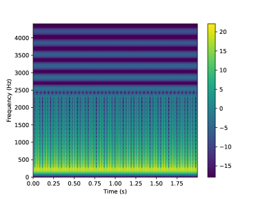
Figure 1: Spectrogram of a harmonic signal involving sine waves with close frequencies in the low frequency range, and sine waves with better separated frequencies in the high frequency range.

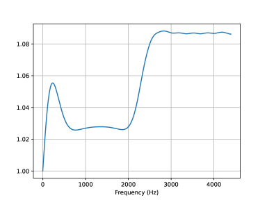
Figure 2: Frequency focus function based upon a ratio $L^{2}/L^{1}$ norms, for the signal whose spectrogram is displayed in Figure 1

The prototypical frequency focus function introduced in (20) turns out to be insufficient to produce the expected behaviour, because of spurious oscillations (not shown here). The latter can be suppressed by appropriate low-pass filtering. After such filtering and normalisation, on obtains a focus function as given in Figure 2. The latter can be suitably rescaled to match a prescribed range, and thresholded to achieve the support property assumed in its definition. Since it is not the objective of this paper to provide realistic choices for applications, we d’on’t address such a fine tuning here.

As can be seen on Figure 2, the frequency focus function takes lower values in the low-frequency part of the signal spectrum. This implies that the window in the frequency-focused transform will have larger scale, therefore smaller frequency bandwidth, which will provide the desired adaptation to the signal if the aim is to better separate sine waves.

Remark A.33.

Other more explicit illustrations can also be obtained since all calculations rely on Gaussian integrals which are tractable. In our opinion this does not bring more insight than the numerical examples in the Appendix, we then refrain from following this avenue.

A.2 An example of time focus function

We now revisit Example 4.23, and illustrate the behaviour of a time focus function similar to (51) on another toy example, consisting in coloured noise with additional randomly located spikes with random amplitude. A realisation of such a random signal (involving 10 random peaks, out of which some are not visible because they are hidden by the background noise) is plotted in Figure 3. Its spectrogram (not shown here) exhibits a clear frequency decay (as a result of the choice of noise) away from the spike locations (which do not decay in the frequency domain). The time focus function used here is designed to capture such a behaviour, which we illustrate below.

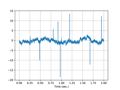
Figure 3: Gaussian coloured noise with randomly located spikes, with random amplitudes.

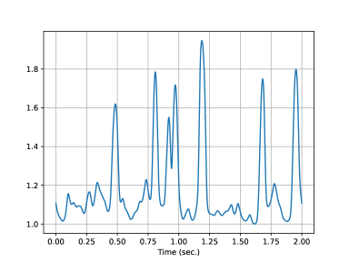
Figure 4: Time focus function for the spike+noise signal plotted in Figure 3.

We display in Figure 4 the corresponding time focus function, as defined in (51). The focus function presents clear maxima near 7 time instants, which turn out to coincide with the locations of the 7 neatly visible spikes (out of 10 generated spikes, the other 3 having smaller amplitude). The function was rescaled to achieve the prescribed minimal value of 1; again further post-processing is possible to achieve the support condition of the definition, we refrained from doing it as this would require an extra thresholding parameter, such a fine tuning being irrelevant at this stage.

References

- \bibcommenthead
- Daubechies [1992] Daubechies, I.: Ten Lectures on Wavelets. CBMS-NSF Regional Conference Series in Applied Mathematics, vol. 61. Society for Industrial and Applied Mathematics, USA (1992). https://doi.org/10.1137/1.9781611970104.fm
- Gröchenig [2013] Gröchenig, K.: Foundations of Time-frequency Analysis. Springer, Boston, MA (2013). https://doi.org/10.1007/978-1-4612-0003-1
- Grossmann and Morlet [1984] Grossmann, A., Morlet, J.: Decomposition of Hardy functions into square integrable wavelets of constant shape. SIAM Journal on Mathematical Analysis 15(4), 723–736 (1984) https://doi.org/10.1137/0515056
- Mallat [2008] Mallat, S.: A Wavelet Tour of Signal Processing, Third Edition: The Sparse Way. Academic Press, Inc., USA (2008). https://doi.org/10.1016/B978-0-12-374370-1.X0001-8
- Meyer [1993] Meyer, Y.: Wavelets and Operators. Cambridge Studies in Advanced Mathematics, vol. 1. Cambridge University Press, Cambridge, UK (1993). https://doi.org/10.1017/CBO9780511623820
- Kalisa and Torrésani [1993] Kalisa, C., Torrésani, B.: N-dimensional affine Weyl-Heisenberg wavelets. Annales de l’I.H.P. Physique théorique 59(2), 201–236 (1993) https://eudml.org/doc/76620
- Ali et al. [2000] Ali, S.T., Antoine, J.-P., Gazeau, J.-P.: Coherent States, Wavelets and Their Generalizations. Springer, New York, Berlin, Heidelberg (2000). https://doi.org/10.1007/978-1-4614-8535-3
- Fornasier [2007] Fornasier, M.: Banach frames for -modulation spaces. Applied and Computational Harmonic Analysis 22(2), 157–175 (2007) https://doi.org/10.1016/j.acha.2006.05.008
- Stockwell et al. [1996] Stockwell, R.G., Mansinha, L., Lowe, R.P.: Localization of the complex spectrum: the S transform. IEEE Transactions on Signal Processing 44(4), 998–1001 (1996) https://doi.org/10.1109/78.492555
- Brown [1991] Brown, J.C.: Calculation of a constant Q spectral transform. The Journal of the Acoustical Society of America 89(1), 425–434 (1991) https://doi.org/10.1121/1.400476
- Velasco et al. [2011] Velasco, G.A., Holighaus, N., Dörfler, M., Grill, T.: Constructing an invertible constant-Q transform with non-stationary Gabor frames. Proceedings of DAFX11, Paris 33 (2011)
- Folland and Sitaram [1997] Folland, G.B., Sitaram, A.: The uncertainty principle: A mathematical survey. Journal of Fourier Analysis and Applications 3, 207–238 (1997) https://doi.org/10.1007/BF02649110
- Ricaud and Torrésani [2013] Ricaud, B., Torrésani, B.: Refined support and entropic uncertainty inequalities. IEEE Transactions on Information Theory 59(7), 4272–4279 (2013) https://doi.org/10.1109/TIT.2013.2249655
- Oxenham [2018] Oxenham, A.J.: How we hear: The perception and neural coding of sound. Annual Review of Psychology 69(1), 27–50 (2018) https://doi.org/10.1146/annurev-psych-122216-011635 . PMID: 29035691
- Oppenheim and Magnasco [2013] Oppenheim, J.N., Magnasco, M.O.: Human time-frequency acuity beats the Fourier uncertainty principle. Phys. Rev. Lett. 110, 044301 (2013) https://doi.org/10.1103/PhysRevLett.110.044301
- Brandenburg [1999] Brandenburg, K.: MP3 and AAC Explained. In: Audio Engineering Society Conference: 17th International Conference: High-Quality Audio Coding (1999). http://www.aes.org/e-lib/browse.cfm?elib=8079
- Holighaus et al. [2012] Holighaus, N., Dörfler, M., Velasco, G.A., Grill, T.: A framework for invertible, real-time constant-Q transforms. IEEE Transactions on Audio, Speech, and Language Processing 21(4), 775–785 (2012) https://doi.org/10.1109/TASL.2012.2234114
- Conway [2019] Conway, J.B.: A Course in Functional Analysis. Graduate Texts in Mathematics, vol. 96. Springer, New York, Berlin, Heidelberg (2019). https://doi.org/10.1007/978-1-4757-4383-8
- Dahlke et al. [2008] Dahlke, S., Fornasier, M., Rauhut, H., Steidl, G., Teschke, G.: Generalized coorbit theory, banach frames, and the relation to -modulation spaces. Proceedings of the London Mathematical Society 96(2), 464–506 (2008) https://doi.org/10.1112/plms/pdm051 https://londmathsoc.onlinelibrary.wiley.com/doi/pdf/10.1112/plms/pdm051
- Molla and Torrésani [2004] Molla, S., Torrésani, B.: Determining local transientness of audio signals. IEEE Signal Processing Letters 11(7), 625–628 (2004) https://doi.org/10.1109/LSP.2004.830110
- Wei [2020] Wei, W.H.: On the development of nonlinear operator theory. Functional Analysis and Its Applications 54, 49–52 (2020) https://doi.org/10.1134/S0016266320010062
- Balazs et al. [2011] Balazs, P., Dörfler, M., Jaillet, F., Holighaus, N., Velasco, G.: Theory, implementation and applications of nonstationary Gabor frames. Journal of Computational and Applied Mathematics 236(6), 1481–1496 (2011) https://doi.org/10.1016/j.cam.2011.09.011
- Dörfler and Matusiak [2015] Dörfler, M., Matusiak, E.: Nonstationary Gabor frames - approximately dual frames and reconstruction errors. Advances in Computational Mathematics 41(2), 293–316 (2015) https://doi.org/10.1007/s10444-014-9358-z
- Arrivault and Jaillet [2018] Arrivault, D., Jaillet, F.: The Large Time-Frequency Toolbox (LTFAT) in Python. https://pypi.org/project/ltfatpy/. LabEx Archimede, LIS, I2M, Aix-Marseille Université. Accessed: 2023-06-20 (2018)
- Průša et al. [2014] Průša, Z., Søndergaard, P.L., Holighaus, N., Wiesmeyr, C., Balazs, P.: The Large Time-Frequency Analysis Toolbox 2.0. In: Sound, Music, and Motion. LNCS, pp. 419–442. Springer, New York, Berlin, Heidelberg (2014). https://doi.org/10.1007/978-3-319-12976-1_25