Neural State-Dependent Delay Differential Equations

Abstract

Discontinuities and delayed terms are encountered in the governing equations of a large class of problems ranging from physics, engineering, medicine to economics. These systems are impossible to be properly modelled and simulated with standard Ordinary Differential Equations (ODE), or any data-driven approximation including Neural Ordinary Differential Equations (NODE). To circumvent this issue, latent variables are typically introduced to solve the dynamics of the system in a higher dimensional space and obtain the solution as a projection to the original space. However, this solution lacks physical interpretability. In contrast, Delay Differential Equations (DDEs) and their data-driven, approximated counterparts naturally appear as good candidates to characterize such complicated systems. In this work we revisit the recently proposed Neural DDE by introducing Neural State-Dependent DDE (SDDDE), a general and flexible framework featuring multiple and state-dependent delays. The developed framework is auto-differentiable and runs efficiently on multiple backends. We show that our method is competitive and outperforms other continuous-class models on a wide variety of delayed dynamical systems.

[1] organization=Université Paris-Saclay, CNRS, addressline=Laboratoire Interdisciplinaire des Sciences du Numérique, postcode=91405, city=Orsay, country=France

[2] organization=Université Paris-Saclay, CNRS, Inria, addressline=Laboratoire Interdisciplinaire des Sciences du Numérique, postcode=91405, city=Orsay, country=France

1 Introduction

In many applications, one assumes the time-dependent system under consideration satisfies a Markov property; that is, future states of the system are entirely defined from the current state and are independent of the past. In this case, the system is satisfactorily described by an ordinary or a partial differential equation. However, the principle of Markovianity is often only a first approximation to the true situation and a more realistic model would include past states of the system. Describing such systems has fueled the extensive development of the theory of delay differential equations (DDE) (Minorsky, 1942; Myshkis, 1949; Hale, 1963). This development has given rise to many practical applications: in the modelling of molecular kinetics (Roussel, 1996) as well as for diffusion processes (Epstein, 1990), in physics for modeling semiconductor lasers (Vladimirov et al., 2004), in climate research for describing the El Ninõ current (Ghil et al., 2008; Keane et al., 2019) and tsunami forecasting (Wu et al., 2022), to list only a few.

At the same time, the blooming of machine learning in recent years boosted the development of new algorithms aimed at modelling and predicting the behaviour of dynamical systems governing phenomena commonly found in a wide variety of fields ranging from physics to engineering or medicine. Among these novel strategies, the introduction of Neural Ordinary Differential Equations (NODEs) (Chen et al., 2018) has contributed to further deepening the analysis of continuous dynamical systems modelling based on neural networks. Indeed, NODEs are a family of neural networks that can be seen as the continuous extension of Residual Networks (He et al., 2016), where the dynamics of a vector – hereafter often identified with the state of a physical system – $\mathbf{x}(t)\in\mathbb{R}^{d}$ at time $t$ is given by the parameterized network $\mathbf{f}_{\theta}$:

$$\frac{d\mathbf{x}(t)}{dt}\equiv\dot{\mathbf{x}}(t)=\mathbf{f}_{\theta}(\mathbf{x}(t),t),\quad\mathbf{x}(0)=\mathbf{x}_{0}.$$ (1)

NODEs have been successfully applied to various tasks, such as normalizing flows (Kelly et al., 2020; Grathwohl et al., 2018), handling irregularly sampled time data (Rubanova et al., 2019; Kidger et al., 2020), and image segmentation (Pinckaers and Litjens, 2019).

Table 1: Comparison with existing works that deals with DDEs. Our implementation deals with a wider range of delays

delay types	$\tau$’s definition	Neural DDE	NPCDDEs	Neural Laplace	Neural SDDDE
References	-	Zhu et al. (2021)	Zhu et al. (2022)	Holt et al. (2022)	This work
Constant	$\tau=a$	$\surd$	$\times$	$\surd$	$\surd$
Piece-wise constant	$\tau=\lfloor\frac{t-a}{a}\rfloor a$	$\times$	$\surd$	$\surd$	$\surd$
Time-dependent	$\tau=f(t)$	$\times$	$\times$	$\surd$	$\surd$
State-Dependent	$\tau=f(t,x(t))$	$\times$	$\times$	$\times$	$\surd$
Continuous	$\tau=\int_{0}^{t}f(s,x(s))ds$	$\times$	$\times$	$\times$	$\times$

1.1 Related works

Starting from this groundbreaking work, numerous extensions of the NODE framework enabled to extend the range of applications; among them, the augmented version, usually referred to as Augmented Neural ODEs (ANODEs) by Dupont et al. (2019), was able to alleviate NODEs’ expressivity bottleneck by augmenting the dimension of the space allowing the model to learn more complex functions using simpler flows (Dupont et al., 2019). Let $\mathbf{a}(t)\in\mathbb{R}^{p}$ denotes a point in the augmented space, the ODE problem is formulated as

$$\frac{d}{dt}\begin{bmatrix}\mathbf{x}(t)\\ \mathbf{a}(t)\end{bmatrix}=\mathbf{f}_{\theta}\left(\begin{bmatrix}\mathbf{x}(t)\\ \mathbf{a}(t)\end{bmatrix},t\right),\quad\begin{bmatrix}\mathbf{x}(0)\\ \mathbf{a}(0)\\ \end{bmatrix}=\begin{bmatrix}\mathbf{x}_{0}\\ \mathbf{0}\end{bmatrix}.$$ (2)

By introducing this new variable $\mathbf{a}(t)$ ANODE overcomes the inability of NODE to represent particular classes. However, this comes with the cost of lifting the data into a higher dimensional space, hence losing its interpretability. Among the techniques proposed for circumventing the limitations rising from the modelling of non-Markovian systems, the Neural Laplace model (Holt et al., 2022) proposes a unified framework that solves differential equations (DE): it learns DE solutions in the Laplace domain. The Neural Laplace model cascades 3 steps: first a network $\mathbf{h}_{\gamma}$ encodes the trajectory, then the so-called Laplace representation network $\mathbf{g}_{\beta}$ learns the dynamics in the Laplace domain to finally map it back to the temporal domain with an inverse Laplace transform (ILT). With the state $\mathbf{x}$ sampled $T$ times at arbitrary time instants, $\mathbf{h}_{\gamma}$ gives a latent initial condition representation vector $\mathbf{p}\in\mathbb{R}^{K}$:

$$\mathbf{p}=\mathbf{h}_{\gamma}((\mathbf{x}(t_{1}),t_{1}),\dots,(\mathbf{x}(t_{T}),t_{T})),$$ (3)

that is fed to the network $\mathbf{g}_{\beta}$ to get the Laplace transform

$$\mathbf{F}(\mathbf{s})=v\left(\mathbf{g}_{\beta}(\mathbf{p},u(\mathbf{s}))\right),$$ (4)

with $u$ a stereographic projector and $v$ its inverse. Ultimately, an ILT step is applied to reconstruct state $\widehat{\mathbf{x}}$ from the learnt $\mathbf{F}(\mathbf{s})$.

1.2 Delay differential equations through neural networks and present work

In alternative to the aforementioned techniques, one may directly attack the DDE problem by working within the framework of neural network-based DDEs. Despite the success of the NODEs philosophy, the extension to DDEs has barely been studied yet, possibly owing to the challenges in applying backpropagation through DDE solvers due to the discontinuities. Very recently, Zhu et al. (2021) first introduced a neural network based DDE with one single constant delay:

$$\dot{\mathbf{x}}(t)=\mathbf{f}_{\theta}(t,\mathbf{x}(t),\mathbf{x}(t-\tau)),\quad\tau\in\mathbb{R}$$ (5)

$$\mathbf{x}(t<0)=\mathbf{\phi}(t),$$

where $\phi(t)$ is the system’s history function, $\tau$ a constant delay and $\mathbf{f}_{\theta}$ a parameterized network. Soon after, the same authors proposed Neural Piece-Wise Constant Delays Differential Equations (NPCDDEs) model in Zhu et al. (2022), where the problem is defined as

$$\dot{\mathbf{x}}(t)=\mathbf{f}_{\theta_{k}}(t,\mathbf{x}(t),\mathbf{x}(t-\lfloor\frac{t-\beta_{1}}{\beta_{1}}\rfloor\beta_{1}),\dots,\mathbf{x}(t-\lfloor\frac{t-\beta_{k}}{\beta_{k}}\rfloor\beta_{k}),\quad$$ (6)

$$\mathbf{x}(t<0)=\mathbf{\phi}(t),\quad\forall i\in\{1,2,\ldots,k\},\,\beta_{i}\in\mathbb{R}.$$

Compared to NODE and its augmented counterpart, neural network-based DDEs do not require an augmentation to a higher dimensional space in order to be a universal approximator, thus preserving physical interpretability of the state vector and allowing the detection of the time delays. Nonetheless, the current declination of Neural DDE models only deals with a single constant delay or several piece-wise constant delays, thus lacking generalization since it does not handle arbitrary delays. Moreover, to the best of our knowledge, no machine learning library or open-sourced code exists to model not only these very specific types of DDEs but also any generic DDEs.

In this work, we introduce Neural State-Dependent DDE (SDDDE) model: an open-source, robust python DDE solver . Neural SDDDE is written in JAX (which is auto-differentiable and hardware agnostic) and is based on a general framework that pushes the envelope of Neural DDEs by handling DDEs with several delays in a more generic way. The implementation further encompasses general time- and state-dependent delay systems which extends the reach of Zhu et al. (2022).

In the remainder of the paper, we briefly introduce the framework in §2, together with a brief overview of the algorithms. Implementation and methodologies are further discussed in §3. Experiments and comparisons with the state-of-the-art techniques are detailed in 4, using as benchmark numerous time-delayed models of incremental complexity. Our solver is shown below to compare favorably with the current models on DDEs systems. Conclusions and outlook finalize the article in §5.

2 Neural State-Dependent DDEs

In this section, we present the Neural State-Dependent DDE (SDDDE) model, which can handle multiple types of delays. It is important to note that this approach is not capable of handling delays that are continuous in the sense of delays that are expressed with integrals as can be found in integro-differential equations. The types of delays that can be handled are listed in Table 1. We add that $f$ defined in Table 1 must be a scalar valued function.

2.1 Definition

We now formally introduce the family of Neural SDDDEs. Such a system is defined as

$$\dot{\mathbf{x}}(t)=\mathbf{f}_{\theta}(t,\mathbf{x}(t),\mathbf{x}(t-\tau_{1}),\dots,\mathbf{x}(t-\tau_{k}))$$ (7)

$$\tau_{i}=\tau_{i}(t,\mathbf{x}(t)),\quad\forall i\in[1,2,\ldots,k]$$

$$\mathbf{x}(t<0)=\mathbf{\phi}(t),$$

where $\mathbf{\phi}:\mathbb{R}^{-}\rightarrow\mathbb{R}^{d}$ is the history function, $\tau_{i}:\mathbb{R}\times\mathbb{R}^{d}\rightarrow\mathbb{R}$ a delay function and $\mathbf{f}_{\theta}:[0,T]^{k}\times\mathbb{R}^{d}\rightarrow\mathbb{R}^{d}$ a parameterized network. Most of the time, $\mathbf{f}_{\theta}$, $\tau_{i}$ and $\mathbf{\phi}$ have additional properties like smoothness. By differential order of an equation we mean the order of the highest derivative and by difference order we mean one less than the number of distinct arguments involved (Bellman and Cooke, 1963). Hence, Eq. (7) is of first differential order and $k$ difference order. For a complete overview of DDE theory we refer the reader to Bellen and Zennaro (2013) and Bellman and Cooke (1963).

2.2 Challenges with DDE integration

Three problems arise in DDEs that can cause numerical difficulties. First, discontinuities may occur in various derivatives of the solution. This is due to the presence of delayed terms. In general, there is a derivative jump (or breaking point) at the initial time point $t=0$ since

$$\dot{\mathbf{\phi}}(t=0^{-})\neq\dot{\mathbf{x}}(t=0^{+})\;.$$

Moreover, the history function $\phi$ may also have discontinuities. Discontinuities can then arise and propagate from the history function and initial point (by a discontinuity, we mean a jump in $\boldsymbol{\mathbf{x}}$ or one of its derivatives). Second, a delay may vanish wtih time, i.e., $\tau_{i}\rightarrow 0$. This issue may force the solver to take too many small steps. Authors from Zivari-Piran and Enright (2010) transform the DDE problem into a discontinuous initial value problem (IVP). This enables the problem to transfer ODE properties like uniqueness, existence, stiffness and bounds to DDEs. Third, a delay can be negative and make the integration scheme implicit.

As seen above DDEs can yield discontinuities because of the nature of the history function $\phi$ and the initial time point $t=0$. This shows that DDEs possess a richer dynamical structure than ODEs. The presence of delayed terms may drastically change the qualitative behavior of the solution and act as a stabilizer as well as a destabilizer for models governed by ODEs, linking DDEs to control theory (Kiss and Röst, 2017).

2.3 Uniqueness and existence of solutions to DDEs

For clarity, we now state Bellman’s theorem proving existence and uniqueness of solution to DDEs with constant delays. This result can be adapted to time-dependent delays (Balachandran, 1989) and to the more general case of state-dependent delays (Driver, 1962).

Theorem 1.

Bellman and Cooke (1963) — Local existence
Suppose that $\phi(t)$ is continuous for $0\leq t\leq\omega$, with $m_{\phi}=\max_{0\leq t\leq\omega}\left|\phi(t)\right|$, and that $f(u,v)$ satisfies a Lipschitz condition

$$\left|f(u_{1},v_{1})\right|+\left|f(u_{2},v_{2})\right|<c_{4}(\left|u_{1}-u_{2}\right|+\left|v_{1}-v_{2}\right|)$$ (8)

for $(u_{1},v_{1})$ and $(u_{2},v_{2})$ in a region $N$ such that

$$N:\left|u\right|+\left|v\right|\leq c_{1}\;.$$

Let $c_{2}$ denote the maximum of the (continuous) function $\left|f(u,v)\right|$ for $(u,v)$ in $N$. Then if $2m_{\phi}<c_{1}$, there exists a unique continuous solution $x(t)$ of

$$\dot{x}(t)=f(x(t),x(t-\omega)),\quad t>\omega$$ (9)

$$x(t)=\phi(t),\quad 0\leq t\leq\omega$$

for $0\leq t\leq\omega+c_{3}$, where $c_{3}<(c_{1}-2m_{\phi})/2c_{2}$.

Proof of such a theorem can be found in the book of Bellman and Cooke (1963). The richer structure of DDEs comes with the price of not having a global existence theorem like ODEs, unless requiring certain additional hypotheses.

2.4 Pseudo code for DDE solver

The pseudo code of the DDE solver implemented by Zivari-Piran and Enright (2010) is detailed in Algorithm 1, where the general outline of one integration step of a DDE is shown; the DDE solver is illustrated in Algorithm 2. For sake of simplicity, we suppose for the pseudo code a single time delay DDE since the general case does not differ from it.

2.5 Reverse-mode automatic differentiation of DDE solutions

Backpropagation remains the most challenging technicality when training continuous-depth networks. Authors of Zivari-Piran and Enright (2010) model DDEs as a discontinuous initial value problem (IVP). This approach is also followed in Julia’s implementation (Widmann and Rackauckas, 2022). We follow the same idea of seeing DDEs as several different ODEs defined on specific time intervals that follow one another. This way of thinking allows us to use off-the-shelf ODE solvers as long as discontinuity points are consistently detected during integration. Finally, writing the DDE solver within an auto-differentiable framework allows to train neural networks via gradient descent.

Algorithm 1 Pseudo code for one DDE numerical integration step

  Input: Vector field $\mathbf{f}(t,\mathbf{x},\mathbf{x}(t-\tau))$ Integration bound $t_{n}$, $t_{n+1}$ Interpolated estimated solution $\hat{\mathbf{x}}(t)$ in $[t_{0};t_{n}]$ Set of detected discontinuities $\Lambda=\{\lambda_{-m},\dots,\lambda_{0},\dots,\lambda_{r}\}$.

  if $t_{n+1}-t_{n}>\min(\Lambda)$ then

     Declare the interpolant $\Pi_{n}=\hat{\mathbf{x}}$ of $\mathbf{x}(t-\tau)$ in $[t_{n};t_{n+1}]$

     while the interpolant $\Pi_{n}$ has not converged do

        Define $\mathbf{f}_{\rm ODE}(t,\mathbf{x})=\mathbf{f}(t,\mathbf{x},\Pi_{n}(t))$

        Step the solver $\mathbf{x}(t_{n+1})=ODESolve(\hat{\mathbf{x}}(t_{n}),\mathbf{f}_{\rm ODE},t_{n},t_{n+1})$

        Update $\Pi_{n}$ using the computed solution $\mathbf{x}(t_{n+1})$.

     end while

  else

     Define $\mathbf{f}_{\rm ODE}(t,\mathbf{x})=\mathbf{f}(t,\mathbf{x},\hat{\mathbf{x}}(t-\tau))$

     Step the solver $\mathbf{x}(t_{n+1})=ODESolve(\hat{\mathbf{x}}(t_{n}),\mathbf{f}_{\rm ODE},t_{n},t_{n+1})$

  end if

  Determine next time step $t_{\text{next}}$ from solver

  if step is accepted then

     Return updated $\hat{\mathbf{x}}(t)$, next integration bounds $t_{n+1},t_{\text{next}}$ and $\Lambda$.

  else

     Check for discontinuities in $[t_{n};t_{n+1}]$

     if a discontinuity is found, $\lambda_{r+1}$ then

        Return same $\hat{\mathbf{x}}(t)$, next integration bounds $t_{n},\lambda_{r+1}$ and $\Lambda\cup\{\lambda_{r}\}$ .

     else

        Return same $\hat{\mathbf{x}}(t)$, next integration bounds $t_{n}$, $t_{next}$ and $\Lambda$.

     end if

  end if

  Output: Interpolated estimated solution Next integration bounds Updated set of discontinuities

Algorithm 2 Pseudo code for DDE solver

  Input: Vector field $\mathbf{f}(t,\mathbf{x},\mathbf{x}(t-\tau))$ Integration bound $t_{0}$, $t_{F}$ History function $\phi(t)$ Set of initial discontinuities $\Lambda=\{\lambda_{-m},\dots,\lambda_{0}\}$.

  Choose an initial $dt$

  Declare $t_{n}=t_{0},t_{n+1}=t_{0}+dt$

  Declare interpolated estimated solution $\hat{\mathbf{x}}(t)=\phi(t)$ in $[t_{n};t_{n+1}]$

  repeat

     Algorithm 1

  until $t_{n+1}=t_{F}$

3 Methods

In the following, we discuss similarities, drawbacks and benefits of Neural SDDDE compared with the following models: NODE, ANODE and Neural Laplace. Compared to these techniques, we recall that Neural SDDDE is a direct method for solving DDEs, specifically designed to handle delayed systems; it does not require lifting of the problem to higher-dimensional spaces, with the benefit of preserving physical interpretability. This is not the case for ANODE, the augmented version of ODE, where flexibility is obtained by introducing an higher dimentional space. Lastly, Neural Laplace can solve a broader class of differential equations, although with some limitations that we pinpoint in the following.

3.1 Model comparison

From the theoretical viewpoint, the Laplace transformation is often a tool used in proofs on DDEs (Bellman and Cooke, 1963) since it allows to transform linear functional equations in $\mathbf{f}(\mathbf{x}(t))$ involving derivative and differences into linear equations involving only $\mathbf{F}(\mathbf{s})$. Thus, time-dependent and constant delay DDEs are transformed into linear equations of $\mathbf{F}(\mathbf{s})$ using the Laplace transform. This transformation enables Neural Laplace to bypass the explicit definition of delays, whereas Neural SDDDE needs the delays to be specified unless the vector flow $\mathbf{f}$ and delays are learnt jointly. These observations tie Neural Laplace to Neural SDDDE as they can be seen as similar models but living in different domains. However, a limitation of Laplace transformation-based approaches is that they are not defined for DDEs with state-dependent delays, thus limiting the class of time-delayed equation that one can solve with this technique.

Neural Laplace is a model that needs memory initialized latent variables, i.e., a long portion of the trajectory needs to be fed in order to get a reasonable representation of the latent variable. In contrast, by design, NODE and ANODE require information only at the initial time to predict the system dynamics. From this viewpoint, Neural SDDDE is somewhat a hybrid approach since a history function $\phi(t)$ is required. $\phi$ needs to be provided for $t\in[-\tau_{\mathrm{max}},0]$, where $\tau_{\mathrm{max}}$ is the maximum delay encountered during integration. This is more restricting than solely relying on an initial condition $\mathbf{x}(0)$ but far less than memory-based latent variables methods. Moreover, the training and testing schemes for Neural Laplace is constrained by this very same observation since future events can only be predicted after a certain observation time. This also makes the length of the trajectory to feed to Neural Laplace a hyperparameter to tune. This is not the case with NODE, ANODE and our approach.

3.2 Memory and computational complexity

Neural SDDDEs rely on an ODE solver, thus function evaluations are associated with the same computational cost as NODEs. However, Neural SDDDE has some extra constraints making the method more computationally involved. Hereafter, we compare the complexity of these two schemes; we define $S$ as the number of stages in the Runge-Kutta (RK) scheme used for the time-integration, $N$ the total number of integration steps, and $d$ the state’s dimension.

Memory complexity

DDE integration necessitates keeping a record of all previous states in memory due to the presence of delayed terms. This is because at any given time $t$, the DDE solver must be able to accurately determine $\mathbf{x}(t-\tau)$ through interpolation of the stored state history. This extra amount of extra memory needed depends on the solver used. For example, the additional memory required when using a RK solver for one trajectory is $O(SNd)$. The model’s memory footprint is not affected by the number of delays.

Time complexity

In comparison to NODE, the solution estimate $\widehat{\mathbf{x}}$ needs to be evaluated for each delayed state argument, i.e., $\mathbf{x}(t-\tau_{i})$. The cost of evaluating the interpolant is small compared to the cost of computing its coefficients. Similarly, the time complexity is conditioned by the solver used. For example, for a RK scheme, the coefficient computation scales linearly with the number of stages. Hence, Neural SDDDE adds a time cost $O(SD\,d)$ compared to NODE for each vector field function evaluation.

4 Experiments

We evaluate and compare the Neural SDDDE on several dynamical systems listed below coming from biology and population dynamics. We show that Neural SDDDE outperforms a variety of continuous-depth models and demonstrates its capabilities in simulating state-dependent delayed systems.

4.1 Dynamical systems

We pick different dynamical systems that exhibit specific delays since it is our main focus. Some systems are taken from Holt et al. (2022) for comparison.

One constant time-delay system

We consider the delayed Lotka-Volterra from Bahar and Mao (2004), that simulates population dynamics:

$$\dot{x}(t)=\frac{1}{2}x(t)(1-y(t-\tau))$$ (10)

$$\dot{y}(t)=-\frac{1}{2}y(t)(1-x(t-\tau)).$$

The delay is fixed to $\tau=0.2$, we integrate in the time range $[0,30]$ and define the constant history function $\phi(t)=(x_{0},y_{0})$ $\forall t<0$ with $x_{0}$ and $y_{0}$ uniformly sampled from $[0.1,2]$.

Chaotic system with one constant time delay

We choose a chaotic setting of the Mackey-Glass system (Mackey and Glass, 1977) that mimics pathological behavior in certain biological contexts:

$$\dot{x}(t)=\beta\frac{x(t-\tau)}{1+x(t-\tau)^{n}}-\gamma x(t),$$ (11)

with $\beta=0.25$, $n=10$ and $\gamma=0.1$. The delay is fixed to $\tau=10$. We integrate in the time range $[0,80]$ and define the constant history function $\phi(t)=x_{0}$ where $x_{0}$ is uniformly sampled from $[0.1,1.0]$.

Time-dependent delay system

Here, the delay is time dependent:

$$\dot{x}(t)=x(t)(1-x(t-\tau(t))),$$ (12)

with $\tau(t)=2+\sin(t)$. We integrate in the time range $[0,40]$ and define the constant history function $\phi(t)=x_{0}$, where $x_{0}$ is uniformly sampled from $[0.1,2.0]$.

State-dependent time-delay system

In this example, we consider the 1-D state-dependent Mackey Glass system from Dads et al. (2022) with a state-dependent delay:

$$\dot{x}(t)=-\alpha(t)x(t)+\beta(t)\frac{x^{2}(t-\tau(x))}{1+x^{2}(t-\tau(x))}+\gamma(t)$$ (13)

$$\text{with}\quad\alpha(t) =4+\sin(t)+\sin(\sqrt{2t})+\frac{1}{1+t^{2}}$$ (14)

$$\beta(t) =\gamma(t)=\sin(t)+\sin(\sqrt{2t})+\frac{1}{1+t^{2}}$$

and $\tau(x)=\frac{1}{2}\cos{x(t)}$. The model is defined on the time range $[0,10]$ and the constant history function is $\phi(t)=x_{0}$ with $x_{0}$ uniformly sampled from $[0.1,1]$.

Delayed Diffusion Equation

Finally, we choose the delayed PDE taken from Arino et al. (2009). Such dynamics can for example model single species growth in a food-limited environment.

$$\frac{\partial u}{\partial t}(x,t)=D\frac{\partial^{2}u}{\partial x^{2}}(x,t)+ru(x,t)\left(1-u(x,t-\tau)\right),$$ (15)

where $D=0.01,r=0.9$ and $\tau=2$. We integrate in the time range $[0,4]$, the spatial domain is $\mathcal{D}_{x}=[0,1]$ with periodic boundary conditions and define the history function $\phi(x,t)=a\sin{x}e^{-0.01t}$ where $a$ is uniformly sampled from $[0.1,4.0]$. The spatial mesh is created with $dx=0.01$.

Data generation

For all the systems listed in this section, data generation information is gathered in  C along with information of the step history function generation in D.

	NODE	ANODE	Neural Laplace	Neural SDDDE
Lokta-Volterra	$.00288\pm.00148$	$.0132\pm.0081$	$.275\pm.178$	$\mathbf{.00265\pm.00074}$
Mackey-Glass	$.668\pm 1.22$	$.00355\pm.00383$	$.0123\pm.0093$	$\mathbf{.000159\pm.000189}$
Time Dependent DDE	$1.01\pm.435$	$.00729\pm.00235$	$.0144\pm.0037$	$\mathbf{.00148\pm.00087}$
State-Dependent DDE	$.0363\pm.0015$	$.00107\pm.00076$	$.00379\pm.00110$	$\mathbf{.000149\pm.000007}$
Delay Diffusion	$.00117\pm.00020$	$.000200\pm.000052$	$\mathbf{.0000737\pm.0000106}$	$.000300\pm.000043$

Table 2: Test MSE averaged over 5 runs of each experiments with their standard deviation. Best result bolded.

4.2 Evaluation

We assess the performance of the models with their ability to predict future states of a given system. The metric used is the mean square error (MSE) in all cases. Neural Laplace predicts only after a burn-in time since a part of the observed trajectory is used to learn a latent initial condition vector $\mathbf{p}$. Since NODE, ANODE and Neural SDDDE can be seen as initial value problems (IVPs) we produce trajectories from initial conditions and compute the MSE with respect to the whole trajectory. On each DDE system, to judge the quality of each model, we elaborate two additional experiments alongside with the test set predictions. By modifying the history function $\phi(t)$ we change the behavior of the system and hence generate new trajectories. The first experiment puts each model in a pure extrapolation regime ; the constant value of the history function $\phi(t)=\mathbf{x}_{0}$ is sampled outside the range of the training and testing data. This allows to see the models’ extrapolation capabilities. The second assessment is more a hybrid approach where the history function is a step function:

$$\phi(t) =\begin{cases}\mathbf{x}_{0}&t\leq t_{\text{jump}}\\ \mathbf{x}_{1}&\text{otherwise}\end{cases}$$

$$t_{\text{jump}} \sim\mathcal{U}(-\tau_{\text{max}},0),\quad\mathbf{x}_{0},\mathbf{x}_{1}\sim\mathcal{U}(c_{0},c_{1})$$

where $t_{\text{jump}}$ is the largest delay in the system and $c_{0},c_{1}$ are system specific randomly sampled values (see D for more details). Not only can the nature of the history step function change but can also have its domain function outside of the training and test data (extrapolation regime).

As a reminder, to produce outputs, NODE and ANODE need an initial condition, Neural SDDDE the history function and Neural Laplace a portion of the trajectory. To ensure comparison in our experiments, we opt to give Neural Laplace the same information as Neural SDDDE, specifically the history function. This could be seen as a restriction of Neural Laplace since in its authors give 50% of the trajectory to produce outputs. Therefore, we propose another small experiment: on one dynamical system, Neural SDDDE is compared with Neural Laplace which is given more than just the history function.

As stated previously, Neural Laplace does not need to define delays thanks to the Laplace transformation compared to Neural SDDDE. This is why we provide one last experiment: for the Mackey-Glass system, several delays are provided to the vector field of Neural SDDDE. The model will have to learn the system’s dynamics with the panel of provided delays.

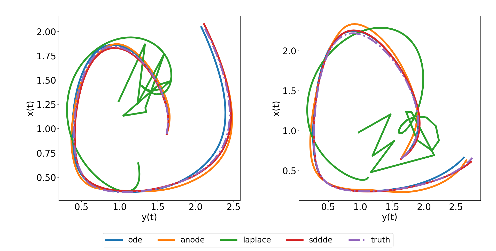
(a) Lotka Volterra randomly sampled test trajectory plots

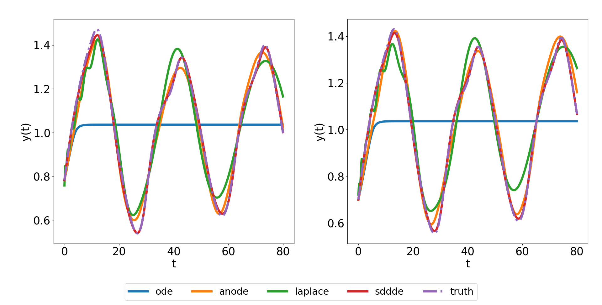
(b) Mackey-Glass randomly sampled test trajectory plots

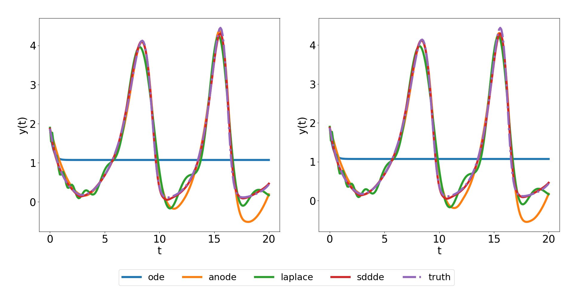
(c) Time Dependent DDE randomly sampled test trajectory plots

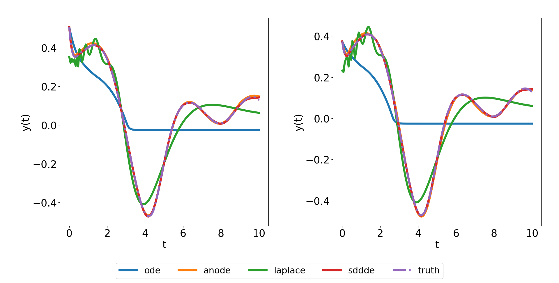
(d) State Dependent DDE randomly sampled test trajectory plots

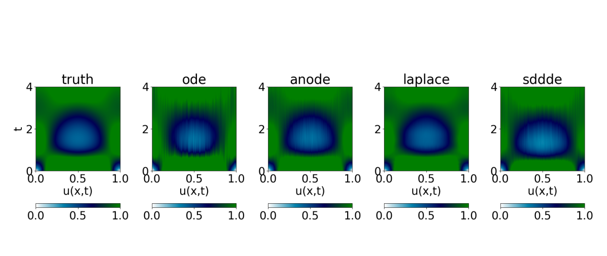
(e) Diffusion Delay PDE randomly sampled from the testset

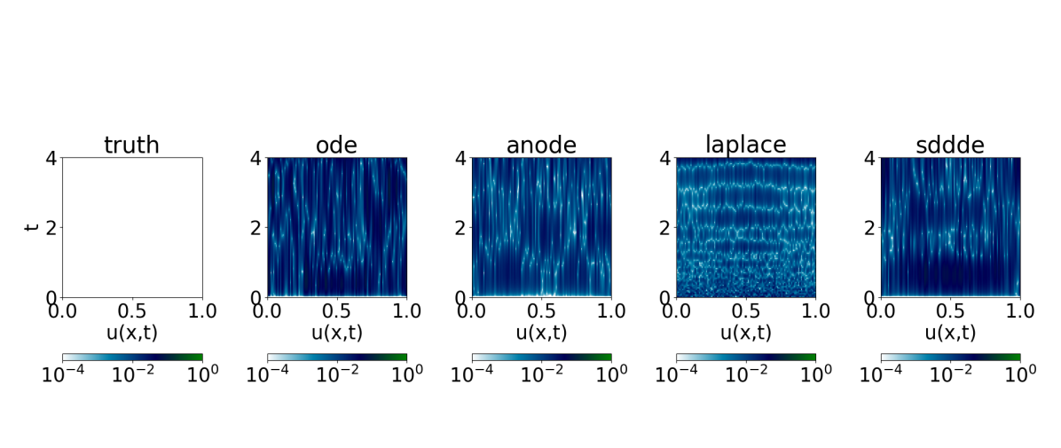
(f) Absolute error of Diffusion Delay PDE randomly sampled from the testset

Figure 1: Randomly test trajectory plots of Lotka-Volterra, Mackey-Glass, Time, State Dependent DDEs and Diffusion Delay PDE

4.3 Results

Test errors for each experiments are reported in Table 2. Complementary information are included in the Appendix References for what concerns the implementation and the training process; training curves are plotted in  A, model and training hyperparameters are given in B.

Testset prediction

Neural SDDDE almost consistently outperforms each model over all DDE systems mentioned in section 4 and plots are provided with Figure 1. Neural Laplace seems to suffer from the Runge phenomenon where its most evident example is the State-Dependent DDE (Figure 1(d)) but also in the Mackey-Glass DDE (Figure 1(b)). This is most likely due to the query algorithm that does not span enough the Laplace domain. Not surprisingly, Neural ODE is the most limited model: all over predicts only the dynamics’ mean trajectory of the dynamical systems under consideration except for the Lotka Volterra dataset where it reproduces the correct dynamics (Figure 1(a)). ANODE gives satisfactory results except in the Time Dependent DDE (1(c)). Finally, Neural SDDDE out of all the models provide the best outcome. Regarding the Diffusion Delay PDE, the PDE’s evolution is predicted with an absolute error going as high as $10^{-2}$ with all models as seen in Figure 1(e). The absolute error is also displayed in Figure 1(f): it depicts the discrepancy between models. Neural Laplace yields more errors for a given time steps across all the spatial domain compared to IVP models that have errors more localized in specific spatial regions.

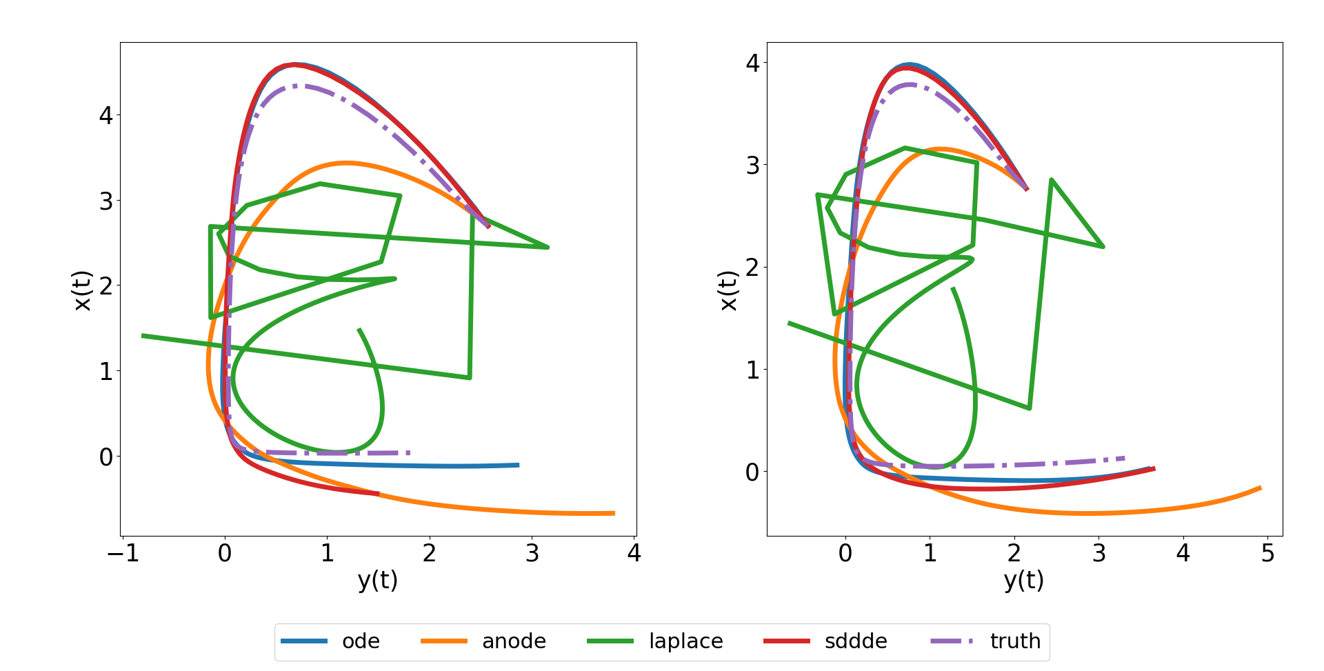
(a) Lotka Volterra randomly sampled extrapolated trajectory plots

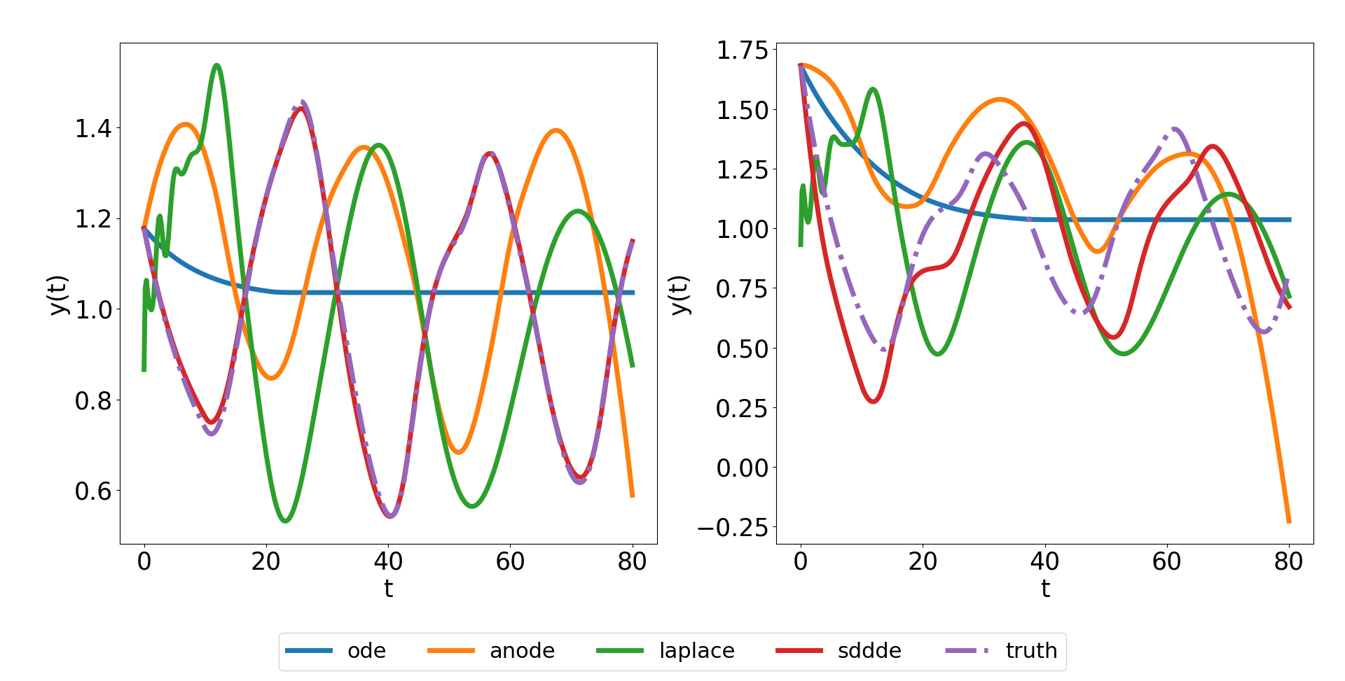
(b) Mackey-Glass randomly sampled extrapolated trajectory plots

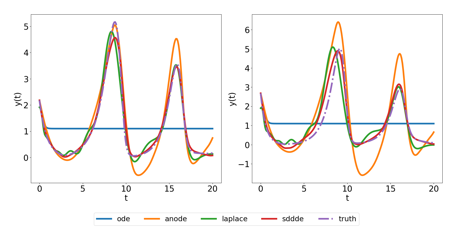
(c) Time Dependent DDE randomly sampled extrapolated trajectory plots

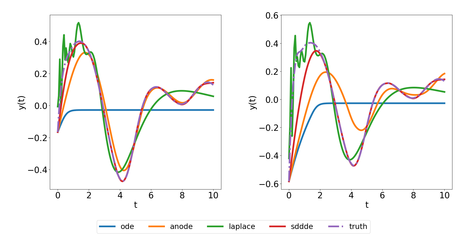
(d) State Dependent DDE randomly sampled extrapolated trajectory plots

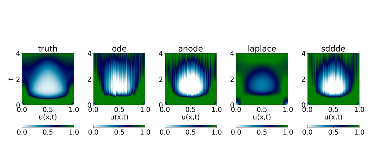
(e) Diffusion Delay PDE randomly sampled from the extrapolated testset

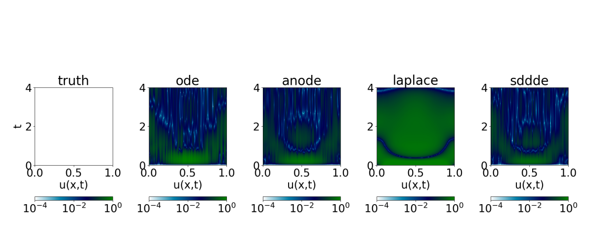
(f) Absolute error of Diffusion Delay PDE randomly sampled from the extrapolated testset

Figure 2: Randomly extrapolated trajectory plots of Lotka-Volterra, Mackey-Glass, Time, State Dependent DDEs and Diffusion Delay PDE

Extrapolation regime prediction

This experiment really challenges model generalization capabilities. Overall, on certain datasets, some models can extrapolate with new constant history functions that are not too far out from the function domain of history functions used during training; more in details, trajectories were generated with $\phi(t)=x_{0}\in[a,b]$: some models are able to exhibit adequate predictions for history functions that have a value near the bounds of $[a,b]$. For example, for the Mackey-Glass system (Figure 2(b)), Neural SDDDE predictions are good up to values of $x_{0}\approx 1.2$. For values higher than $x_{0}\approx 1.4$ (during training $\phi(t)=x_{0}\in[0.1,1]$) overall variations are captured but the amplitudes are off. On the same Figure 2(b), Neural Laplace yields anti-phase results along with what seems to be Runge phenomenon. For the Time Dependent system (Figure 2(c)), Neural Laplace yields better results: trajectories possess the overall dynamical trend with some amplitude discrepancy. Regarding performances of NODE and ANODE, results are quite heterogeneous, most of them fail apart for some exceptions discussed below. For the State-Dependent DDE (Figure 2(d)), ANODE produces satisfactory trajectories. This can be explained because the system at hand has almost periodic solutions thus easier to learn. For the Lotka Volterra dataset (Figure 2(a)), IVP models (ANODE, NODE, Neural SDDDE) across the board yield realistic results even though the system’s dynamics is not captured perfectly. For the Diffusion Delay PDE, overfitting is observed for Neural Laplace. Out of all the IVP models, Neural SDDDE predicts the best possible outcome compared to NODE and ANODE.

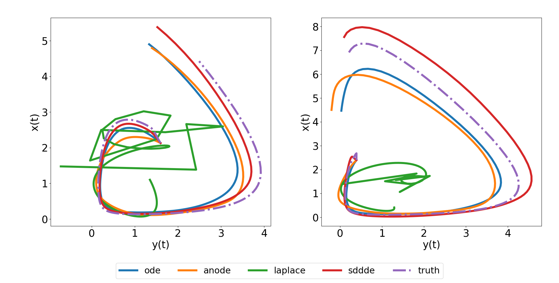
(a) Lotka Volterra randomly sampled from history step function

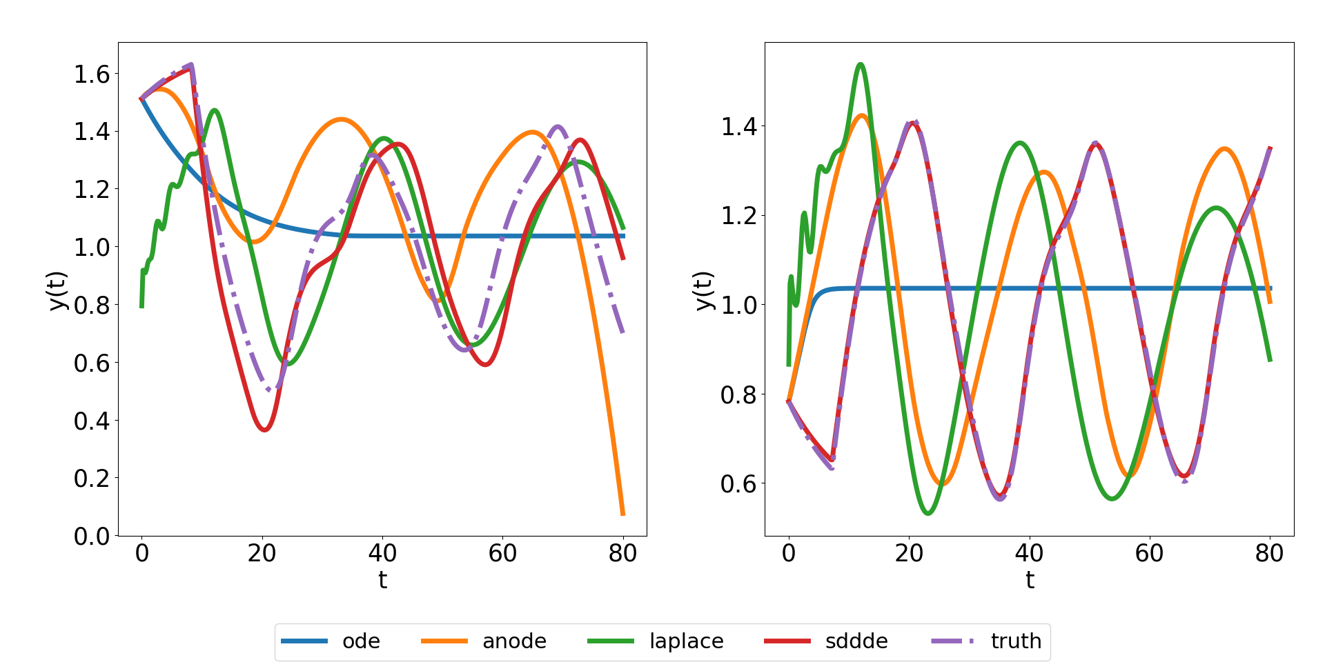
(b) Mackey-Glass randomly sampled from history step function

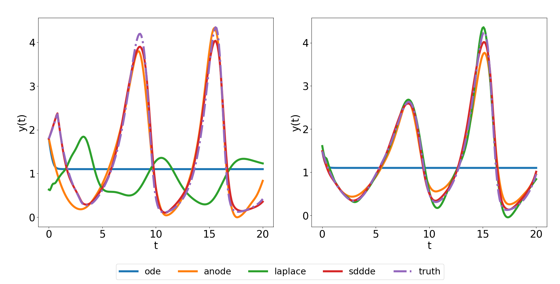
(c) Time Dependent DDE randomly sampled from history step function

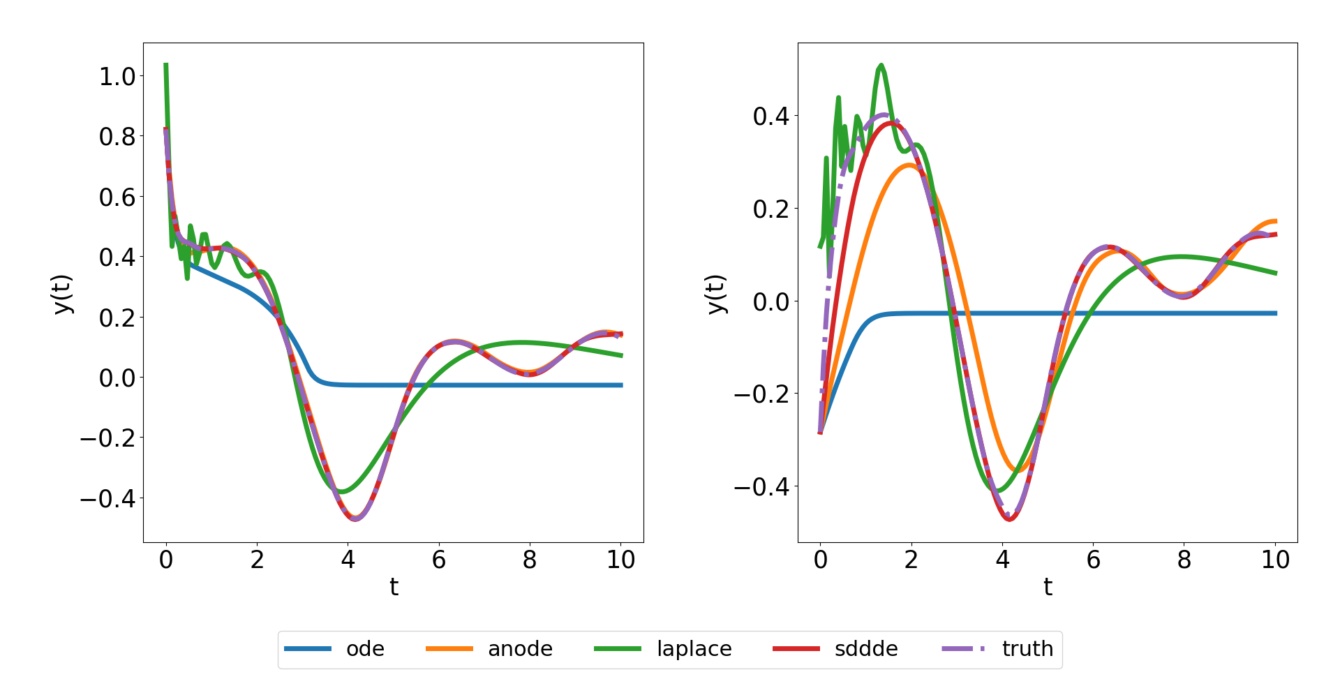
(d) State Dependent DDE randomly sampled from history step function

Figure 3: Randomly sampled trajectory plots from other history step function experiment of Lotka-Volterra, Mackey-Glass, Time, State Dependent DDEs and Diffusion Delay PDE

Step history function prediction

This third experiment also demonstrates how the modification of the history function leads to changes in the transient regime and impacts later dynamics. For example, the plots in Figure 3(b) exhibits a monotonic change at $t\approx 10$ (it appeared because we added a new discontinuity jump in the history function) that never appeared beforehand and Neural SDDDE captures it to some extent. Neural Laplace fails to generate adequate trajectories apart from the State-Dependent DDE already discussed in the previous paragraph. Regarding the other IVP models exhibit the same performance as in the previous paragraph. By studying the effect of such a new history function on the Diffusion Delay PDE, we saw that the system’s dynamics is not changed substantially, therefore, we decided to omit this system’s comparison.

	NODE	ANODE	Neural Laplace	Neural SDDDE
$\alpha=0$	$1.01\pm.435$	$.00729\pm.00235$	$.0144\pm.00368$	$\mathbf{.00148\pm.000872}$
$\alpha=0.02$	$.720\pm.00254$	$.0128\pm.002377$	$.00881\pm.00254$	$\mathbf{.000906\pm.000441}$
$\alpha=0.05$	$4.032\pm 4.225$	$.03655\pm.0349$	$.00977\pm.00146$	$\mathbf{.00250\pm.000951}$
$\alpha=0.1$	$1.597\pm 1.100$	$.0223\pm.00634$	$.0154\pm.00501$	$\mathbf{.0121\pm.00534}$
$\alpha=0.2$	$1.02\pm.282$	$.0321\pm.00319$	$.0273\pm.00704$	$\mathbf{.0186\pm.00524}$

Table 3: Test MSE with the noiseless data averaged over 5 runs of each Time Dependent DDE noise experiments with their standard deviation. Best result bolded.

Increasing trajectory fed for Neural Laplace

In this trial, instead of only giving the history function to Neural Laplace we provide 50% of the trajectory to construct its latent initial condition representation vector $\mathbf{p}$ during training as in its original paper. Thus, the first half of the trajectory is injected in Neural Laplace to predict the second half. We choose to train the model on the Time Dependent DDE along with the same training procedure (see B). We provide the training loss for this new setup in Figure 7 where Neural Laplace achieves the lowest training data. Provided the test MSE of Table 2, we choose to only compare the test MSE of Neural SDDDE and Neural Laplace in Table 4. By comparing Figure 4 and 1(c) one can clearly note that the Runge phenomenon are almost absent and predictions are almost as good as Neural SDDDE. This confirms that, in general, Neural Laplace needs more than the history function in order to correctly simulate DDEs.

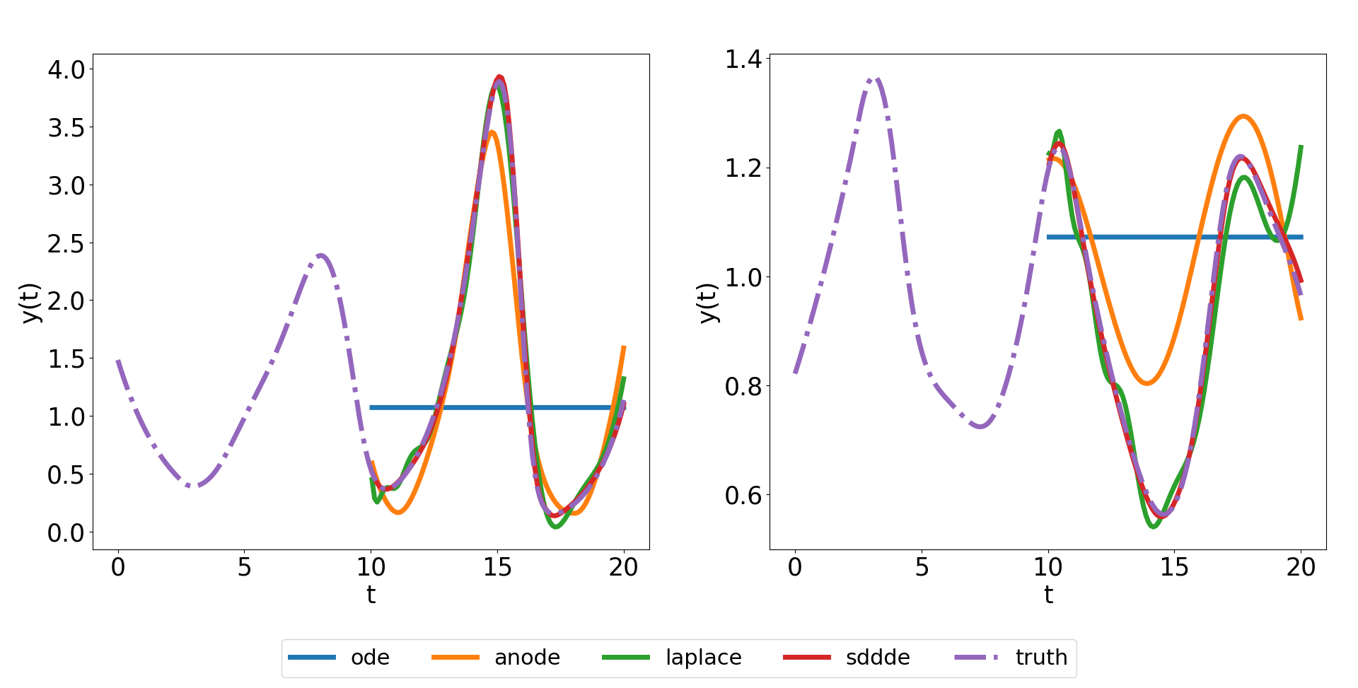
Figure 4: Time-dependent DDE randomly sampled testset trajectories where 50% of data is fed to Neural Laplace

	Neural Laplace	Neural SDDDE
Test MSE	$\mathbf{.000543\pm.000235}$	$.00148\pm.00087$

Table 4: Time Dependent test MSE averaged over 5 runs of each experiments with their standard deviation. Best result bolded.

Noise analysis

We conduct a noise study on one of the datasets, the Time Dependent DDE system. Each data point is added Gaussian noise that is scaled with a certain factor $\alpha$ of the trajectory’s variance. The model is then trained with this noisy data and evaluated on the noiseless testset. In our experiment, we selected 4 scaling factors $\alpha$: $0.02,0.05,0.1$ and $0.2$. Results in Table 3 show that our model is robust to noisy data and almost consistently outperforms other models. Additionally, results from Table 3 show that adding a small amount of noise (here $\alpha=0.02$) makes the learning process more robust, a common result in Machine Learning (Morales et al., 2007; You et al., 2019).

Giving several delays to choose from

We now consider the case where Neural SDDDE is instantiated with a certain number of delays but only a subset of them correspond to the delayed terms of the system considered in hand. Figure 5 demonstrates that Neural SDDDE is able to provide accurate dynamics for the Mackey-Glass DDE where the delays provided were $\left\{5.0,10.0,15.0\right\}$ (The training procedure is the same as depicted in B).

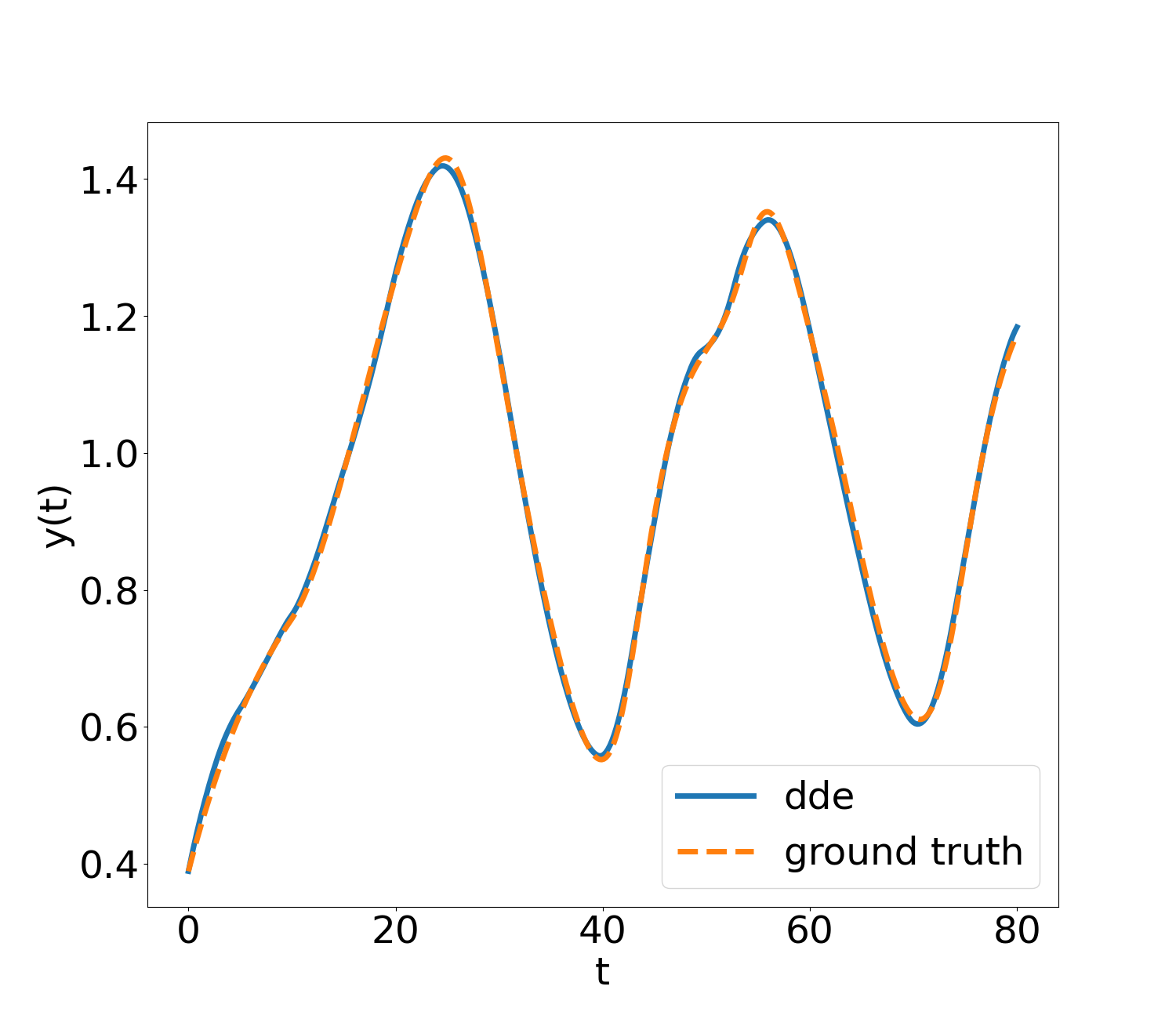
Figure 5: Randomly sampled test set of Mackey-Glass system where several delays were provided

5 Conclusion and Future work

In this paper, we introduced Neural State-Dependent Delays Differential Equations (Neural SDDDE), an auto-differentiable framework for solving Delay Differential Equations (DDEs) with multiple and state-dependent delays via neural networks. This open-source, robust python DDE solver is written in JAX, hardware agnostic and pushes the current envelope of Neural DDEs by handling the delays in a more generic way. To the best of our knowledge, no machine learning library or open-sourced code are available to model in general fashion DDEs.

The need for such a tool rises in modelling and prediction of dynamical systems describing real-life problems is apparent. Indeed, many systems are modelled leveraging the Markovianity property, but this is often only an approximation of more realistic descriptions where the effects of past states affect the current ones. So far, standard ways to data-drive dynamical models via neural networks are by circumventing these limitations with lifting the state to a higher dimensional space – for instance applying the augmented version of Neural ODE (ANODE) – or considering different paradigms such as Neural Laplace. From the theoretical viewpoint, with respect to ANODEs, Neural DDEs preserve physical interpretability of the state vector and allow the detection of the time delays. With respect to Neural Laplace, a technique encompassing a broad number of different DEs, Neural DDEs are capable of handling delays that are state-dependent and do not necessitate a large amount of data for the initialization of the training. Finally, as already mentioned, the current toolbox generalizes the current envelope of DDEs, where only a single constant delay or several piece-wise constant delays can be handled.

In this work, NODEs, the augmented version ANODE and Neural Laplace are used for benchmarking Neural SDDDE using several numerical experiments of incremental complexity, including the Lokta-Volterra and Mackey-Glass models, time- and state- dependent models, and a system characterized by delay diffusion. The dynamics of these models is correctly reproduced for all these cases by Neural SDDDE. Moreover, we have shown that Neural SDDDE performs well compared these with established methods in terms of accuracy and reliability, and is highly effective in modeling DDEs, in particular state-dependent ones when given the delays.

In future research, we plan to expand upon this approach by studying an equivalent version of ANODE with Neural SDDDEs, along with the examination of DDEs of neutral type (NDDEs). Moreover, we believe this flexible and versatile tool may provide a valuable contribution to several fields such as control theory where time-delay are often considered. In particular, it may prove useful in learning a model for partially observed systems whose dynamics of observables can be learned, under mild conditions, from their time-history.

Appendix A Training procedure

Each model is trained with the hyperparameters in B. Loss curves averaged over 5 runs are displayed for each experiment. Plots are with semi-log scales.

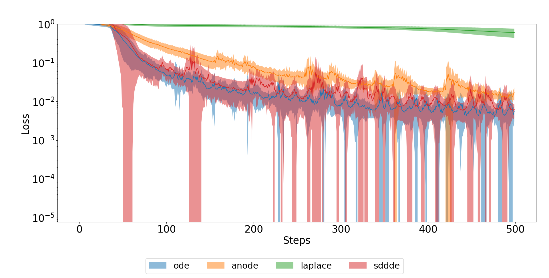
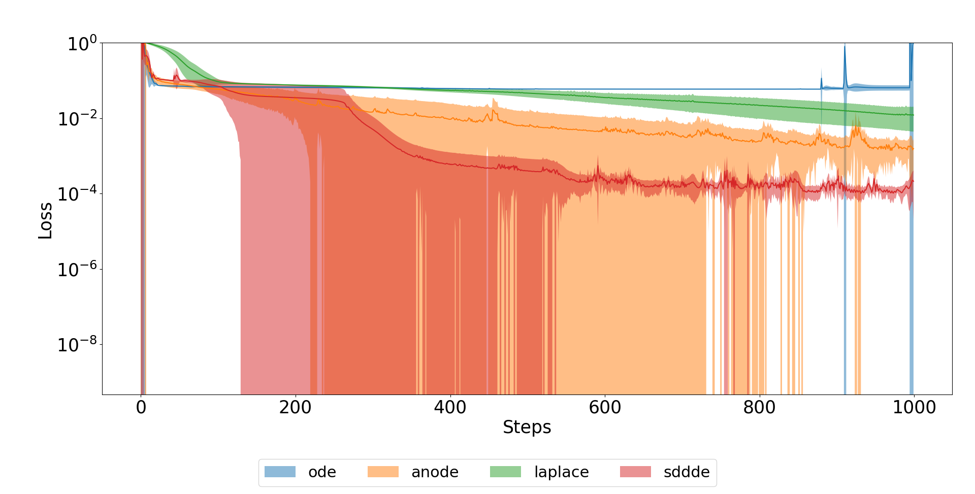
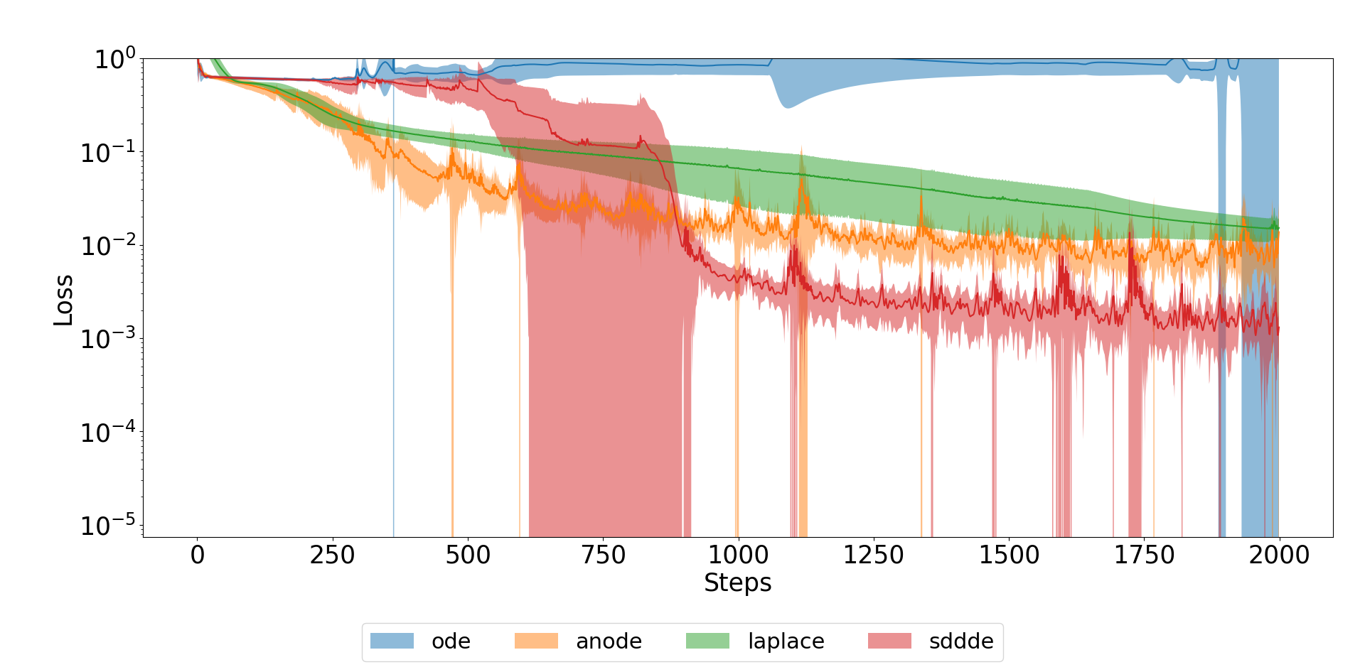
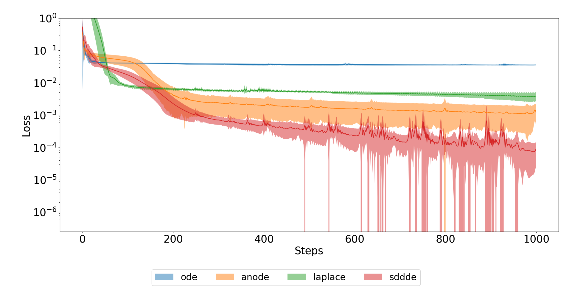
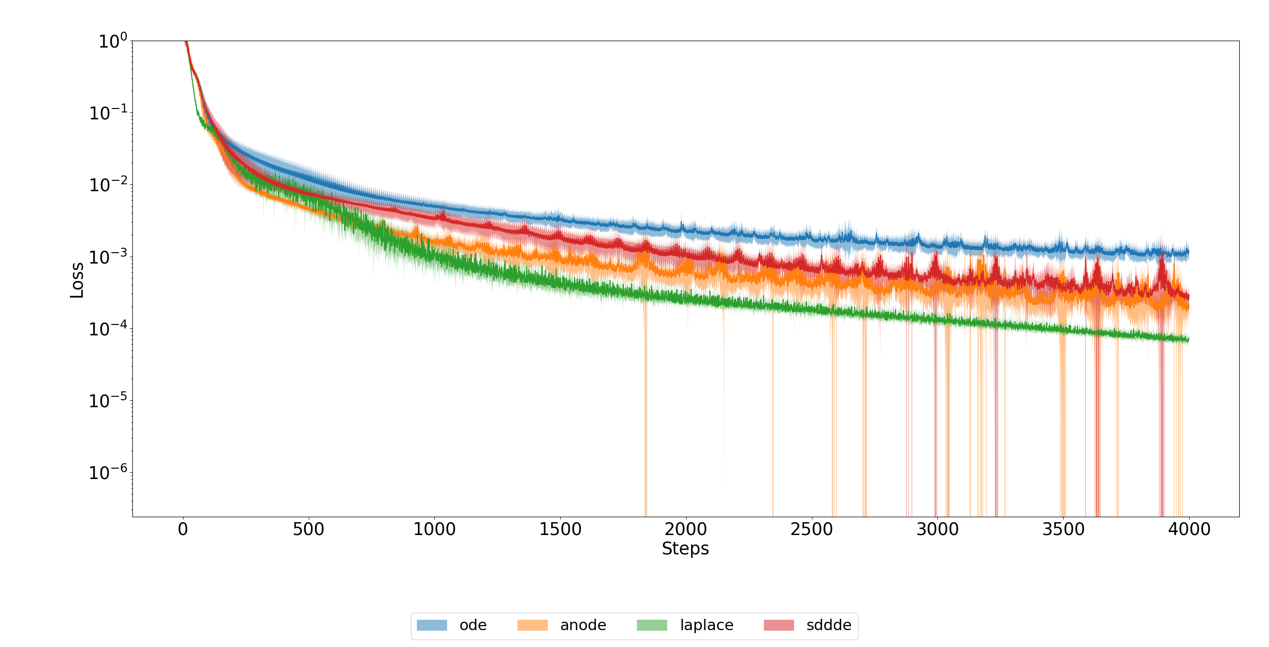
Figure 6: Training losses for all experiments (Lotka Volterra, Mackey-Glass, Time Dependent DDE, State Dependent DDE and Diffusion Delay PDE)

We provide the training loss of Neural Laplace where 50% of the trajectory is fed to the model in Figure 7.

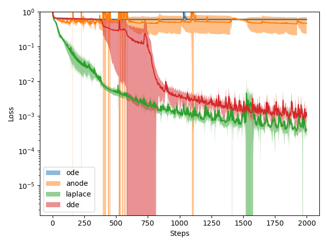
Figure 7: Time Dependent DDE training curve where 50% of data is fed to Neural Laplace

Appendix B Model hyperparameters

Table 5 sums up the MLP architecture of each IVP model (ie NODE, ANODE and Neural DDE) for each dynamical systems. ANODE has an arbitrary augmented state of dimension 10 except for the PDE that has 100. Neural Laplace’s architecture is the default one taken from the official implementation for all systems. The learning rate and the number of epochs are the same for all models. The optimizer used is AdaBelief (Zhuang et al., 2020). Table 6 gives the number of parameters for each model.

	width	depth	activation	epochs	$l_{r}$
Lokta-Volterra	64	3	relu	500	.001
Mackey-Glass	64	3	relu	1000	.001
Time Dependent DDE	64	3	relu	2000	.001
State Dependent DDE	64	3	relu	1000	.001
Diffusion PDE DDE	128	3	relu	500	.0001

Table 5: Model and training hyperparameters

	NODE	ANODE	Neural DDE	Neural Laplace
Lokta-Volterra	8642	9958	8771	17194
Mackey-Glass	8513	9815	8578	17194
Time Dependent DDE	8513	9815	8578	17194
State Dependent DDE	8513	9815	8642	17194
Diffusion PDE DDE	58852	84552	71653	17194

Table 6: Number of parameters for each DDE system

Appendix C Data generation parameters

We expose in Table 7 the parameters used for each dataset generation. The start integration time is always $T_{0}=0$. $T_{F}$ refers to the end time integration. NUM_STEPS equally spaced points are sampled in $[T_{0},T_{F}]$. The specific delays DELAYS and the constant history function $\phi(t)$ function domain are given. Each training dataset is comprised of $256$ datapoints and the testset of $32$ datapoints. We used our own DDE solver to generate the data (Dopri5 ODE solver (Dormand and Prince, 1980) was used.). We then double-checked and compared its validity with Julia’s DDE solver .$\mathcal{U}$ refers to the uniform distribution. For example, Mackey Glass’ constant history function value is uniformly sampled between 0.1 and 1.0. For the Diffusion Delay PDE the history function value in the column $\phi(t)$ refers to the constant $a$ defined in Section 4.1.

	$T_{F}$	num_steps	delays	$\phi(t)$
Lokta-Volterra	15.0	200	0.2	$\mathcal{U}(0.1,2.0)$
Mackey-Glass	80.0	400	10.0	$\mathcal{U}(0.1,1.0)$
Time Dependent DDE	20.0	200	$2\sin(t)$	$\mathcal{U}(0.1,2.0)$
State Dependent DDE	10.0	150	$0.5\cos(\mathbf{x}(t))$	$\mathcal{U}(0.1,1.0)$
Diffusion PDE DDE	4.0	100	$1.0$	$\mathcal{U}(0.1,4.0)$

Table 7: Dataset generation information

Appendix D Experiment parameters for history step function

In table 8 we give the parameters used for each experiment. EXTRAPOLATED $\phi(t)$ indicates the possible value of the constant history function (first experiment). $\tau_{\text{max}}$ and $c_{0},c_{1}$ are described in evaluation’s section 4.2 (second experiment). For the Diffusion Delay PDE, as stated in Section 4.2, the other history step function is omitted. Figure 8 clearly shows how the modification of the history function can drastically change the nature of the dynamics.

	extrapolated $\phi(t)$	$\tau_{\text{max}}$	$c_{0}$	$c_{1}$
Lokta-Volterra	$\mathcal{U}(2.0,3.0)$	$0.2$	$0.1$	$3.0$
Mackey-Glass	$\mathcal{U}(1.0,2.0)$	$10.0$	$0.1$	$2.0$
Time Dependent DDE	$\mathcal{U}(2.0,3.0)$	$3.0$	$0.1$	$3.0$
State Dependent DDE	$\mathcal{U}(-1.0,0.1)$	$1/2$	$-1.0$	$1.0$

Table 8: System specific values for each testing experiment

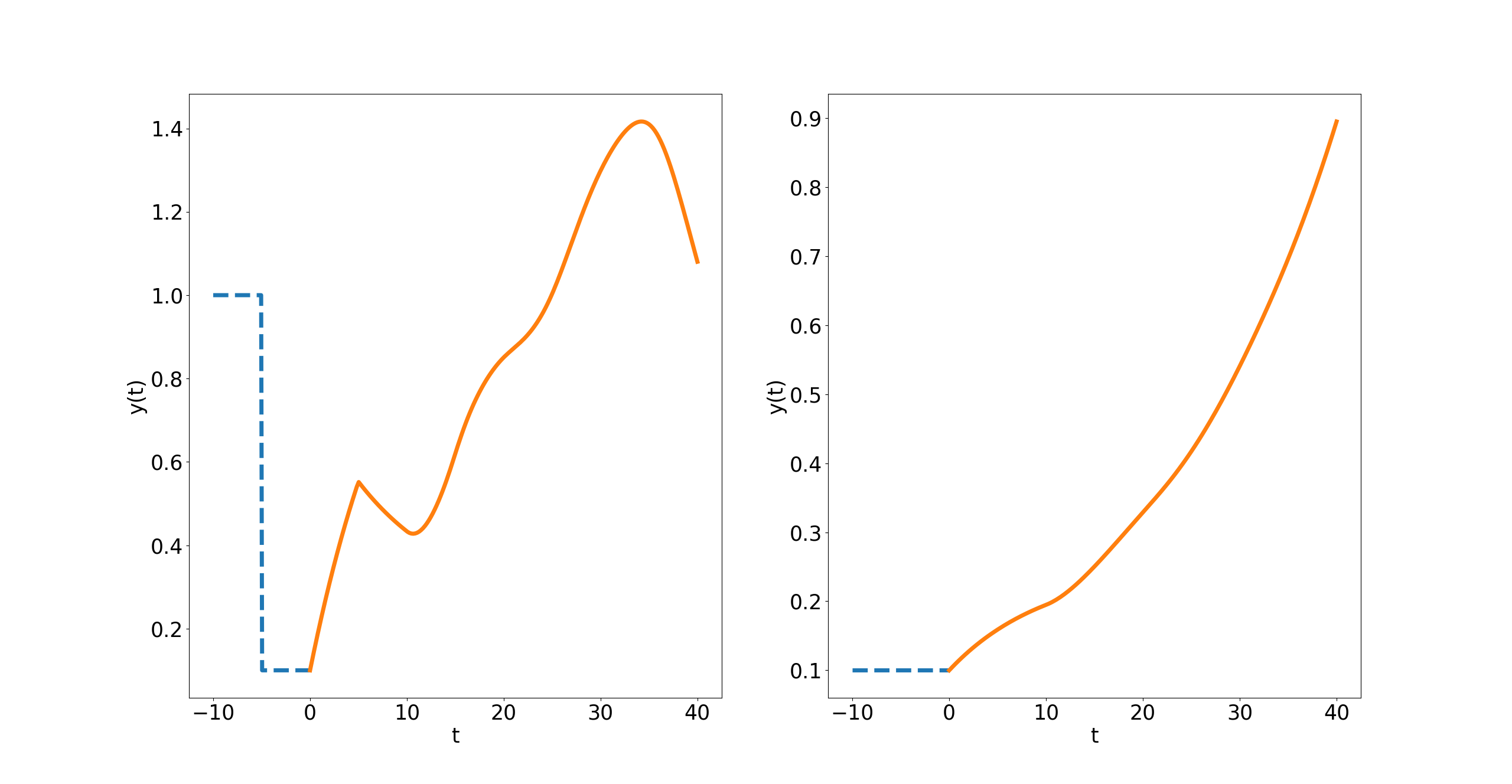
Figure 8: Different history functions (dotted blue line) for Mackey Glass system

References

- Arino et al. (2009) Arino, O., Hbid, M., Dads, E., 2009. Delay Differential Equations and Applications: Proceedings of the NATO Advanced Study Institute held in Marrakech, Morocco, 9-21 September 2002. Nato Science Series II:, Springer Netherlands.
- Bahar and Mao (2004) Bahar, A., Mao, X., 2004. Stochastic delay Lotka–Volterra model. Journal of Mathematical Analysis and Applications 292, 364–380.
- Balachandran (1989) Balachandran, K., 1989. An existence theorem for nonlinear delay differential equations. Journal of Applied Mathematics and Simulation 2, 85–89.
- Bellen and Zennaro (2013) Bellen, A., Zennaro, M., 2013. Numerical methods for delay differential equations. Oxford University Press.
- Bellman and Cooke (1963) Bellman, R.E., Cooke, K.L., 1963. Differential-Difference Equations. RAND Corporation, Santa Monica, CA.
- Chen et al. (2018) Chen, R.T., Rubanova, Y., Bettencourt, J., Duvenaud, D.K., 2018. Neural ordinary differential equations. Advances in neural information processing systems 31.
- Dads et al. (2022) Dads, E.A., Es-sebbar, B., Lhachimi, L., 2022. Almost periodicity in time-dependent and state-dependent delay differential equations. Mediterranean Journal of Mathematics 19, 259.
- Dormand and Prince (1980) Dormand, J.R., Prince, P.J., 1980. A family of embedded Runge-Kutta formulae. Journal of computational and applied mathematics 6, 19–26.
- Driver (1962) Driver, R.D., 1962. Existence and stability of solutions of a delay-differential system. Archive for Rational Mechanics and Analysis 10, 401–426.
- Dupont et al. (2019) Dupont, E., Doucet, A., Teh, Y.W., 2019. Augmented neural ODEs. Advances in Neural Information Processing Systems 32.
- Epstein (1990) Epstein, I.R., 1990. Differential delay equations in chemical kinetics: Some simple linear model systems. The Journal of Chemical Physics 92, 1702–1712.
- Ghil et al. (2008) Ghil, M., Zaliapin, I., Thompson, S., 2008. A delay differential model of ENSO variability: parametric instability and the distribution of extremes. Nonlinear Processes in Geophysics 15, 417–433.
- Grathwohl et al. (2018) Grathwohl, W., Chen, R.T., Bettencourt, J., Sutskever, I., Duvenaud, D., 2018. Ffjord: Free-form continuous dynamics for scalable reversible generative models.
- Hale (1963) Hale, J.K., 1963. A stability theorem for functional-differential equations. Proceedings of the National Academy of Sciences 50, 942–946.
- He et al. (2016) He, K., Zhang, X., Ren, S., Sun, J., 2016. Deep residual learning for image recognition, in: Proceedings of the IEEE conference on computer vision and pattern recognition, pp. 770–778.
- Holt et al. (2022) Holt, S.I., Qian, Z., van der Schaar, M., 2022. Neural Laplace: Learning diverse classes of differential equations in the Laplace domain, in: International Conference on Machine Learning, PMLR. pp. 8811–8832.
- Keane et al. (2019) Keane, A., Krauskopf, B., Dijkstra, H.A., 2019. The effect of state dependence in a delay differential equation model for the El Niño southern oscillation. Philosophical Transactions of the Royal Society A 377, 20180121.
- Kelly et al. (2020) Kelly, J., Bettencourt, J., Johnson, M.J., Duvenaud, D.K., 2020. Learning differential equations that are easy to solve. Advances in Neural Information Processing Systems 33, 4370–4380.
- Kidger et al. (2020) Kidger, P., Morrill, J., Foster, J., Lyons, T., 2020. Neural controlled differential equations for irregular time series, in: Advances in Neural Information Processing Systems, pp. 6696–6707.
- Kiss and Röst (2017) Kiss, G., Röst, G., 2017. Controlling Mackey–Glass chaos. Chaos: An Interdisciplinary Journal of Nonlinear Science 27, 114321.
- Mackey and Glass (1977) Mackey, M.C., Glass, L., 1977. Oscillation and chaos in physiological control systems. Science 197, 287–289. doi:10.1126/science.267326.
- Minorsky (1942) Minorsky, N., 1942. Self-excited oscillations in dynamical systems possessing retarded actions. Journal of Applied Mechanics .
- Morales et al. (2007) Morales, N., Gu, L., Gao, Y., 2007. Adding noise to improve noise robustness in speech recognition, in: Proceedings of the Annual Conference of the International Speech Communication Association, INTERSPEECH, pp. 930–933. doi:10.21437/Interspeech.2007-335.
- Myshkis (1949) Myshkis, A.D., 1949. General theory of differential equations with retarded arguments. Uspekhi Matematicheskikh Nauk 4, 99–141.
- Pinckaers and Litjens (2019) Pinckaers, H., Litjens, G., 2019. Neural ordinary differential equations for semantic segmentation of individual colon glands.
- Roussel (1996) Roussel, M.R., 1996. The use of delay differential equations in chemical kinetics. The Journal of Physical Chemistry 100, 8323–8330.
- Rubanova et al. (2019) Rubanova, Y., Chen, R., Duvenaud, D., 2019. Latent ODEs for irregularly-sampled time series (2019).
- Vladimirov et al. (2004) Vladimirov, A.G., Turaev, D., Kozyreff, G., 2004. Delay differential equations for mode-locked semiconductor lasers. Optics letters 29, 1221–1223.
- Widmann and Rackauckas (2022) Widmann, D., Rackauckas, C., 2022. DelayDiffEq: Generating delay differential equation solvers via recursive embedding of ordinary differential equation solvers.
- Wu et al. (2022) Wu, F., Hong, S., Rim, D., Park, N., Lee, K., 2022. Mining causality from continuous-time dynamics models: An application to tsunami forecasting. arXiv:2210.04958.
- You et al. (2019) You, Z., Ye, J., Li, K., Xu, Z., Wang, P., 2019. Adversarial noise layer: Regularize neural network by adding noise, in: 2019 IEEE International Conference on Image Processing (ICIP), pp. 909–913.
- Zhu et al. (2021) Zhu, Q., Guo, Y., Lin, W., 2021. Neural delay differential equations. arXiv:2102.10801.
- Zhu et al. (2022) Zhu, Q., Shen, Y., Li, D., Lin, W., 2022. Neural piecewise-constant delay differential equations. arXiv:2201.00960.
- Zhuang et al. (2020) Zhuang, J., Tang, T., Ding, Y., Tatikonda, S., Dvornek, N., Papademetris, X., Duncan, J.S., 2020. Adabelief optimizer: Adapting stepsizes by the belief in observed gradients. arXiv:2010.07468.
- Zivari-Piran and Enright (2010) Zivari-Piran, H., Enright, W.H., 2010. An efficient unified approach for the numerical solution of delay differential equations. Numerical Algorithms 53, 397–417.