Splitting Approach for Solving Multi-Component Transport Models with Maxwell-Stefan-Diffusion

Abstract

In this paper, we present splitting algorithms to solve multicomponent transport models with Maxwell-Stefan-diffusion approaches. The multicomponent models are related to transport problems, while we consider plasma processes, in which the local thermodynamic equilibrium and weakly ionized plasma-mixture models are given. Such processes are used for medical and technical applications. These multi-component transport modelling equations are related to convection-diffusion-reactions equations, which are wel-known in transport processes. The multicomponent transport models can be derived from the microscopic multi-component Boltzmann equations with averaging quantities and leads into the macroscopic mass, momentum and energy equations, which are nearly Navier-Stokes-like equations. An additional extension of the multicomponent diffusion term is based on the Maxwell-Stefan approach. Such an approach allows to derive a diffusivity matrix, while the molecular force are balanced and relate all individual species velocities. The Maxwell-Stefan diffusion approach is nonlinear, while we need additional balancing equations. Such additional nonlinear equations are solved with iterative schemes. We concentrate on solving the mass conservation equations of the Navier-Stokes-like equations. Here, we consider splitting approaches with non-iterative and iterative schemes. The splitting approaches are effective methods to decompose delicate multicomponent transport models, while the different operators in the transport models can be solved with optimal numerical solvers. We discuss the benefits of the decomposition into the convection, diffusion and reaction parts, which allows to use fast numerical solvers for each part. Additional, we concentrate on the nonlinear parts of the multicomponent diffusion, which can be effectively solved with iterative splitting approaches In the numerical experiments, we see the benefit of combining iterative splitting methods with nonlinear solver methods, while these methods can relax the nonlinear terms. In the outview, we discuss the future investigation of the next steps in our multicomponent diffusion approaches.

Keywords: Splitting approach, Multicomponent Transport Model, Maxwell-Stefan-diffusion, iterative splitting methods, nonlinear solvers.

I Introduction

In this paper, we concentrate on applying splitting approaches to multicomponent transport models with Maxwell-Stefan-Diffusion, [10]. The modelling equations can be derived from the linearized Boltzmann equations with approximated collision-terms to Navier-Stokes-like equations, while we apply the Chapman-Enskog expansion and averaging techniques concerning particle density, particle flux and particle kinetic energy, see [7] and [8].

In our modelling problem, we consider a simplified plasma model, which considers only heavy particles, which can be modelled as following:

The distribution function of the heavy particles are given as $f_{i}({\bf x},{\bf c}_{i},t)$, while ${\bf x}$ is the three-dimensional spatial coordinate, ${\bf c}_{i}$ is the velocity of the molecule and $t$ is the time. The heavy-particle species distribution are given as:

$${\cal D}_{i}(f_{i})={\cal S}_{i}(f_{i})+{\cal C}_{i}(f_{i}),\;i\in I$$ (1)

where ${\cal S}_{i}(f_{i})$ is the scattering source term, ${\cal C}_{i}(f_{i})$ is the reactive source term and ${\cal D}_{i}(f_{i})$ is the differential operator, see [7]. By applying Chapman-Enskog expansion, we apply the first-order perturbed distribution function to the linearized Boltzmann equations and obtain with the averaging quantities of the particle density the macroscopic equation (mass-conservation). The mass conservation is given as:

$$\frac{\partial\rho_{i}}{\partial t}+\nabla_{\mathbb{x}}\cdot(\rho_{i}\mathbb{v})+\nabla_{\mathbb{x}}(\rho_{i}{\cal V}_{i})=m_{i}\omega_{i}^{0},\;i\in I,$$ (2)

while $\rho_{i}$ is the mass density of $i$, ${\mathbb{v}}$ is the mean velocity, ${\cal V}_{i}$ is the species diffusion velocities and $\omega_{i}^{0}$ is the zero-th order production rate of species $i$, see [7].

We apply the Maxwell-Stefan approach and consider 3 species, then the transport model of the species, see the derivation in [2], which is given as:

$$\partial_{t}\xi_{i}-\nabla\cdot({\bf v}\xi_{i})+\nabla\cdot N_{i}=S_{i},\;1\leq i\leq 3,$$ (3)

$$\sum_{j=1}^{3}N_{j}=0,$$ (4)

$$\frac{\xi_{2}N_{1}-\xi_{1}N_{2}}{D_{12}}+\frac{\xi_{3}N_{1}-\xi_{1}N_{3}}{D_{13}}=-\nabla\xi_{1},$$ (5)

$$\frac{\xi_{1}N_{2}-\xi_{2}N_{1}}{D_{12}}+\frac{\xi_{3}N_{2}-\xi_{2}N_{3}}{D_{23}}=-\nabla\xi_{2},$$ (6)

where $\xi_{i}$ are the mole fractions and $N_{i}$ is the molar flux of species $i$, see [1] and [2]. The velocity ${\bf v}$ is given by the Navier-Stokes equation and we assume to deal with a first simplified model with a constant velocity. Furthermore, the kinetic term or reaction term $S_{i}$ is given as:

$$S_{i}=\sum_{j=1}^{3}\lambda_{i,j}\xi_{j},$$ (7)

where $\lambda_{i,j}$ are the reaction-rates. The domain is given as $\Omega\in{I\!\!R}^{d},d\in{I\!\!N}^{+}$ with $\xi_{i}\in C^{2}$.

II Methods

We apply Operator splitting techniques to decompose the delicate full differential equations, see [3] and [4]. We decompose into a diffusion, a reaction and a convection part, see [5] and [6]. We apply the following splitting approach to our problem, we compute $n=1,\ldots,N$, $t_{0},t_{1},\ldots,t_{n}$ time-steps:

• The first step is given as (Diffusion step):

  $$\partial_{t}\tilde{\xi}_{i}+\nabla\cdot N_{i}=0,\;1\leq i\leq 3,\;\mbox{for}\;t\in[t^{n},t^{n+1}],$$ (8)

  $$\sum_{j=1}^{3}N_{j}=0,$$ (9)

  $$\frac{\tilde{\xi}_{2}N_{1}-\tilde{\xi}_{1}N_{2}}{D_{12}}+\frac{\tilde{\xi}_{3}N_{1}-\xi_{1}N_{3}}{D_{13}}=-\nabla\xi_{1},$$ (10)

  $$\frac{\tilde{\xi}_{1}N_{2}-\tilde{\xi}_{2}N_{1}}{D_{12}}+\frac{\tilde{\xi}_{3}N_{2}-\tilde{\xi}_{2}N_{3}}{D_{23}}=-\nabla\tilde{\xi}_{2},$$ (11)

  $$\tilde{\xi}_{i}(t^{n})=\xi_{i}(t^{n}),\;i=1,2,3,\;t\in[t^{n},t^{n+1}],$$ (12)

• the next step is given as (Reaction step):

  $$\partial_{t}\hat{\xi}_{i}=S_{i},\;1\leq i\leq 3,\mbox{for}\;t\in[t^{n},t^{n+1}],$$ (13)

  $$\hat{\xi}_{i}(t^{n})=\tilde{\xi}_{i}(t^{n+1}),\;i=1,2,3.$$ (14)

• and the next step is given as (Convection step):

  $$\partial_{t}\xi_{i}=\nabla\cdot({\bf v}\xi_{i}),\;1\leq i\leq 3,\mbox{for}\;t\in[t^{n},t^{n+1}],$$ (15)

  $$\xi_{i}(t^{n})=\hat{\xi}_{i}(t^{n+1}),\;i=1,2,3.$$ (16)

In the following section, we will discuss the results of the methods in an application.

III Results

We apply model of a hydrogen plasma, see [10], which we have simplified in a mass-transport model. We deal with the species $H,H_{2},H_{2}^{+}$, which we are heavy particles. We take into account the following reactions, which are given as:

$$H_{2}+e\;\underleftrightarrow{\lambda_{1}}\;H_{2}^{+}+2e,$$ (17)

$$H_{2}+e\;\underleftrightarrow{\lambda_{2}}\;2H+e,$$ (18)

where the electron temperature is given as $T_{e}=17400\;[K]$ and the gas temperature values remain constant $T_{h}=600\;[K]$.

The simplified three component system is given as:

$$\partial_{t}\xi_{i}-v\partial_{x}\xi_{i}+\partial_{x}N_{i}=0,\;1\leq i\leq 3,$$ (19)

$$\sum_{j=1}^{3}N_{j}=0,$$ (20)

$$\frac{\xi_{2}N_{1}-\xi_{1}N_{2}}{D_{12}}+\frac{\xi_{3}N_{1}-\xi_{1}N_{3}}{D_{13}}=-\partial_{x}\xi_{1},$$ (21)

$$\frac{\xi_{1}N_{2}-\xi_{2}N_{1}}{D_{12}}+\frac{\xi_{3}N_{2}-\xi_{2}N_{3}}{D_{23}}=-\partial_{x}\xi_{2},$$ (22)

where the domain is given as $\Omega\in{I\!\!R}^{d},d\in{I\!\!N}^{+}$ with $\xi_{i}\in C^{2}$.

The parameters and the initial and boundary conditions used as following:

• $v=0.01$ (means we have a small convection instead of the diffusion)

• $D_{12}=D_{13}=0.833$ (means $\alpha=0$) and $D_{23}=0.168$ (uphill diffusion, semi-degenerated Duncan and Toor experiment)

• $D_{12}=0.0833,D_{13}=0.680$ and $D_{23}=0.168$ (asymptotic behavior, Duncan and Toor experiment)

• $J=140$ (spatial grid points)

• The time-step-restriction for the explicit method is given as:
  $\Delta t\leq(\Delta x)^{2}\max\{\frac{1}{2\{D_{12},D_{13},D_{23}\}}\}$

• The spatial domain is $\Omega=[0,1]$, the time-domain $[0,T]=[0,1]$

• The initial conditions are:

  $$\xi_{1}^{in}(x)=\left\{\begin{array}[]{l l}0.8&\mbox{if}\;0\leq x<0.25,\\ 1.6(0.75-x)&\mbox{if}\;0.25\leq x<0.75,\\ 0.0&\mbox{if}\;0.75\leq x\leq 1.0,\end{array}\right.,$$ (26)

  $$\xi_{2}^{in}(x)=0.2,\;\mbox{for all}\;x\in\Omega=[0,1],$$ (27)

• The boundary conditions are of no-flux type:

  $$N_{1}=N_{2}=N_{3}=0,\mbox{on}\;\partial\Omega\times[0,1],$$ (28)

The numerical solutions of the three hydrogen plasma in experiment 3 with the uphill diffusion 1.

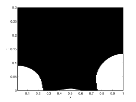
Figure 1: The upper figure presents the result in the space time region, the lower figure presents the the 3D plot of the second component and.

IV Conclusions and Contributions

We present the coupled model for a multi-component transport model simplified plasma processes. The Maxwell-Stefan diffusion approach is considered and solved with additional iterative methods. The nonlinear partial differential equations are splitted into a convection-, diffusion- and reaction part and solved separately with optimal spatial discretization and time-integrator methods. The numerical algorithms are presented and their numerical convergences can be shown, see [6]. Although iterative splitting methods have the benefit of relaxing the nonlinearities and can be used additional with their splitting approaches. They are more accurate than noniterative splitting approaches. The implicit behavior of iterative methods allows larger time-steps to be used and they could accelerate the solver process. In the future we aim to study the numerical analysis of the different combined schemes and enlarge to real-life examples with more species and additional momentum- and energy equations.

References

- [1] D. Bothe. On the Maxwell-Stefan approach to multicomponent diffusion. Parabolic Problems, Progress in Nonlinear Differential Equations and Their Applications, 80, 81–93, 2011
- [2] L. Boudin, B. Grec and F. Salvarani. A mathematical and numerical analysis of the Maxwell-Stefan diffusion equations, Discrete and Continuous Dynamical Systems Series B, 17(5), 1427–1440 2012.
- [3] J. Geiser. Iterative Operator-Splitting Methods with higher order Time-Integration Methods and Applications for Parabolic Partial Differential Equations. Journal of Computational and Applied Mathematics, Elsevier, Amsterdam, The Netherlands, 217, 227-242, 2008.
- [4] J. Geiser. Iterative Splitting Methods for Differential Equations. Chapman & Hall/CRC Numerical Analysis and Scientific Computing Series, edited by Magoules and Lai, 2011.
- [5] J. Geiser. Picard’s iterative method for nonlinear multicomponent transport equations. Cogent Mathematics, 3:1158510, 2016.
- [6] J. Geiser. Multicomponent and Multiscale Systems: Theory, Methods, and Applications in Engineering. Springer International Publishing, Springer International Publishing Switzerland, 2016.
- [7] V. Giovangigli. Multicomponent Flow Modeling. MESST Series. Birkhauser, Boston, 1999.
- [8] V. Giovangigli, B. Graille, T.E. Magin, and M. Massot. Multicomponent transport in weakly ionized mixtures. Plasma Sources Sci. Technol., 19(3):034003, 2010.
- [9] C.T. Kelley. Iterative Methods for Linear and Nonlinear Equations. SIAM Frontiers in Applied Mathematics, no. 16, SIAM, Philadelphia, 1995.
- [10] T.K. Senega and R.P. Brinkmann. A multi-component transport model for non-equilibrium low-temperature low-pressure plasmas. Journal of Physics D: Applied Physics, 39, 1606–1618, 2006.