Design from Policies: Conservative Test-Time Adaptation for Offline Policy Optimization

Abstract

In this work, we decouple the iterative bi-level offline RL (value estimation and policy extraction) from the offline training phase, forming a non-iterative bi-level paradigm and avoiding the iterative error propagation over two levels. Specifically, this non-iterative paradigm allows us to conduct inner-level optimization (value estimation) in training, while performing outer-level optimization (policy extraction) in testing. Naturally, such a paradigm raises three core questions that are not fully answered by prior non-iterative offline RL counterparts like reward-conditioned policy: $\mathtt{Q1}$) What information should we transfer from the inner-level to the outer-level? $\mathtt{Q2}$) What should we pay attention to when exploiting the transferred information for safe/confident outer-level optimization? $\mathtt{Q3}$) What are the benefits of concurrently conducting outer-level optimization during testing? Motivated by model-based optimization (MBO), we propose DROP (Design fROm Policies), which fully answers the above questions. Specifically, in the inner-level, DROP decomposes offline data into multiple subsets and learns an MBO score model ($\mathtt{A1}$). To keep safe exploitation to the score model in the outer-level, we explicitly learn a behavior embedding and introduce a conservative regularization ($\mathtt{A2}$). During testing, we show that DROP permits test-time adaptation, enabling an adaptive inference across states ($\mathtt{A3}$). Empirically, we find that DROP, compared to prior non-iterative offline RL counterparts, gains an average improvement probability of more than 80%, and achieves comparable or better performance compared to prior iterative baselines.

1 Introduction

Offline reinforcement learning (RL) [37, 40] describes a task of learning a policy from static offline data. Due to the overestimation of values at out-of-distribution (OOD) state-actions, recent iterative offline RL methods introduce various policy/value regularization to avoid deviating from the offline data distribution in the training phase. Then, these methods directly deploy the learned policy in an online environment to test its performance. To unfold our following analysis, we term this kind of learning procedure as iterative bi-level offline RL (Figure 1 left), where the inner-level optimization refers to trying to eliminate the OOD issue, the outer-level optimization refers to trying to infer an optimal policy that will be employed at testing. Here, we use the "iterative" term to emphasize that the inner-level and outer-level are iteratively optimized in the training phase. However, due to the iterative error exploitation and propagation [6] over the two levels, performing such an iterative bi-level optimization completely in training often struggles to learn a stable policy/value function.

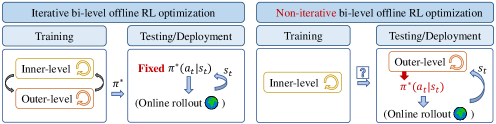
Figure 1: Framework of (iterative and non-iterative) bi-level offline RL optimization, where the inner-level optimization refers to regularizing the policy/value function (for OOD issues) and the outer-level refers to updating the policy for reward maximizing. The "" transferred from inner-level to outer-level depends on the specific choice of algorithm used (see different choices for  in Table 1).

In this work, we thus advocate for non-iterative bi-level optimization (Figure 1 right) that decouples the bi-level optimization from the training phase, i.e., performing inner-level optimization (eliminating OOD) in training and performing outer-level optimization (maximizing return) in testing. Intuitively, incorporating the outer-level optimization into the testing phase can eliminate the iterative error propagation over the two levels, i.e., there is no iteratively learned value function that bootstraps off of itself and thus propagates errors further. Then, three core questions are: $\mathtt{Q1}$) What information ("") should we transfer from the inner-level to the outer-level? $\mathtt{Q2}$) What should we pay special attention to when exploiting "" for safe/confident outer-level optimization? $\mathtt{Q3}$) Notice that the outer-level optimization and the testing rollout form a new loop, what new benefit does this give us?

Intriguingly, prior works under such a non-iterative framework have proposed to transfer ("" in $\mathtt{Q1}$) filtered trajectories [10], a reward-conditioned policy [14, 34], and the Q-value estimation of the behavior policy [6, 24], all of which, however, partially address the above questions (we will discuss these works in Section 3.4). In this work, we thus propose a new alternative method that transfers an embedding-conditioned score model (Q-value) and we will show that this method sufficiently answers the raised questions and benefits most from the non-iterative bi-level framework.

Before introducing our method, we introduce a conceptually similar task (to the non-iterative bi-level optimization) — offline model-based optimization (MBO [62]), which aims to discover, from static input-score pairs, a new design input that will lead to the highest score. Typically, offline MBO first learns a score model that maps the input to its score via supervised regression (corresponding to inner-level optimization), and then conducts inference with the learned score model (as ""), for instance, by optimizing the input against the learned score model via gradient ascent (corresponding to the outer-level). To enable this MBO implementation in offline RL, we are required to decompose an offline RL task into multiple sub-tasks, each of which thus corresponds to a behavior policy-return (parameters-return) pair. However, there are practical optimization difficulties when using high-dimensional policy’s parameter space (as input for the score model) to learn such a score model (inner-level) and conduct inference (outer-level). At inference, directly extrapolating the learned score model ("") also tends to drive the high-dimensional candidate policy parameters towards OOD, invalid, and low-scoring parameters [32], as these are falsely and over-optimistically scored by the learned score model in inner-level optimization.

To tackle these problems, we suggest $\mathtt{A1}$) learning low-dimensional embeddings for those sub-tasks decomposed in the MBO implementation, over which we estimate an embedding-conditioned Q-value ("" in $\mathtt{Q1}$), and $\mathtt{A2}$) introducing a conservative regularization, which pushes down the predicted scores on OOD embeddings. Intuitively, this conservation aims to avoid over-optimistic exploitation and protect against producing unconfident embeddings when conducting outer-level optimization ($\mathtt{Q2}$). Meanwhile, we suggest $\mathtt{A3}$) conducting test-time adaptation, which means we can dynamically adjust the inferred embeddings across testing states (aka deployment adaptation). We name our method DROP (Design fROm Policies). Compared with standard offline MBO for parameter design [62], test-time adaptation in DROP leverages the sequential structure of RL tasks, rather than simply conducting inference at the beginning of testing rollout. Empirically, we demonstrate that DROP can effectively extrapolate a better policy that benefits from the non-iterative framework by answering the raised questions, and achieves better performance compared to state-of-the-art offline RL algorithms.

2 Preliminaries

Reinforcement learning. We model the interaction between agent and environment as a Markov Decision Process (MDP) [61], denoted by the tuple $(\mathcal{S},\mathcal{A},P,R,p_{0})$, where $\mathcal{S}$ is the state space, $\mathcal{A}$ is the action space, $P:\mathcal{S}\times\mathcal{A}\times\mathcal{S}\to[0,1]$ is the transition kernel, $R:\mathcal{S}\times\mathcal{A}\to\mathbb{R}$ is the reward function, and $p_{0}:\mathcal{S}\to[0,1]$ is the initial state distribution. Let $\pi\in\Pi:=\{\pi:\mathcal{S}\times\mathcal{A}\to[0,1]\}$ denotes a policy. In RL, we aim to find a stationary policy that maximizes the expected discounted return $J(\pi):=\mathbb{E}_{\tau\sim\pi}\left[\sum_{t=0}^{\infty}\gamma^{t}R(\mathbf{s}_{t},\mathbf{a}_{t})\right]$ in the environment, where $\tau=\left(\mathbf{s}_{0},\mathbf{a}_{0},r_{0},\mathbf{s}_{1},\mathbf{a}_{1},\dots\right)$, $r_{t}=R(\mathbf{s}_{t},\mathbf{a}_{t})$, is a sample trajectory and $\gamma\in(0,1)$ is the discount factor. We also define the state-action value function $Q^{\pi}(\mathbf{s},\mathbf{a}):=\mathbb{E}_{\tau\sim\pi}\left[\sum_{t=0}^{\infty}\gamma^{t}R(\mathbf{s}_{t},\mathbf{a}_{t})|\mathbf{s}_{0}=\mathbf{s},\mathbf{a}_{0}=\mathbf{a}\right]$, which describes the expected discounted return starting from state $\mathbf{s}$ and action $\mathbf{a}$ and following $\pi$ afterwards, and the state value function $V^{\pi}(\mathbf{s})=\mathbb{E}_{\mathbf{a}\sim\pi(\mathbf{a}|\mathbf{s})}\left[Q^{\pi}(\mathbf{s},\mathbf{a})\right]$. To maximize $J(\pi)$, the actor-critic algorithm alternates between policy evaluation and improvement. Given initial $Q^{0}$ and $\pi^{0}$, it iterates

$$Q^{k+1} \leftarrow\arg\min_{Q}\ \ \mathbb{E}_{(\mathbf{s},\mathbf{a},\mathbf{s}^{\prime})\sim\mathcal{D}^{+},\mathbf{a}^{\prime}\sim\pi^{k}(\mathbf{a}^{\prime}|\mathbf{s}^{\prime})}\left[(R(\mathbf{s},\mathbf{a})+\gamma Q^{k}(\mathbf{s}^{\prime},\mathbf{a}^{\prime})-Q(\mathbf{s},\mathbf{a}))^{2}\right],$$ (1)

$$\pi^{k+1} \leftarrow\arg\max_{\pi}\ \ \mathbb{E}_{\mathbf{s}\sim\mathcal{D}^{+},\mathbf{a}\sim\pi(\mathbf{a}|\mathbf{s})}\left[Q^{k+1}(\mathbf{s},\mathbf{a})\right],$$ (2)

where the value function (critic) $Q(\mathbf{s},\mathbf{a})$ is updated by minimizing the mean squared Bellman error with an experience replay $\mathcal{D}^{+}$ and, following the deterministic policy gradient theorem [59], the policy (actor) $\pi(\mathbf{a}|\mathbf{s})$ is updated to maximize the estimated $Q^{k+1}(\mathbf{s},\pi(\mathbf{a}|\mathbf{s}))$.

Offline reinforcement learning. In offline RL [40], the agent is provided with a static data $\mathcal{D}=\left\{\tau\right\}$ which consists of trajectories collected by running some data-generating policies. Note that here we denote static offline data $\mathcal{D}$, distinguishing from the experience replay $\mathcal{D}^{+}$ in the online setting. Unlike the online RL problem where the experience $\mathcal{D}^{+}$ in Equation 1 can be dynamically updated, the agent in offline RL is not allowed to interact with the environment to collect new experience data. As a result, naively performing policy evaluation as in Equation 1 may query the estimated $Q^{k}(\mathbf{s}^{\prime},\mathbf{a}^{\prime})$ on actions that lie far outside of the static offline data $\mathcal{D}$, resulting in pathological value $Q^{k+1}(\mathbf{s},\mathbf{a})$ that incurs large error. Further, iterating policy evaluation and improvement will cause the inferred policy $\pi^{k+1}(\mathbf{a}|\mathbf{s})$ to be biased towards OOD actions with erroneously overestimated values.

Offline model-based optimization. Model-based optimization (MBO) [63] aims to find an optimal design input $\mathbf{x}^{*}$ with a given score function $f^{*}:\mathcal{X}\to\mathcal{Y}\subset\mathbb{R}$, i.e., $\mathbf{x}^{*}=\arg\max_{\mathbf{x}}f^{*}(\mathbf{x})$. Typically, we can repeatedly query the oracle score model $f^{*}$ for new candidate design, until it produces the best design. However, we often do not have the oracle score function $f^{*}$ but are provided with a static offline dataset $\{(\mathbf{x},y)\}$ of labeled input-score pairs. To track such a design from data question, we can fit a parametric model ${f}$ to the static offline data $\{(\mathbf{x},y)\}$ via the empirical risk minimization (ERM): ${f}\leftarrow\arg\min_{{f}}\mathbb{E}_{(\mathbf{x},y)}\left[\left({f}(\mathbf{x})-y\right)^{2}\right]$. Then, starting from the best point in the dataset, we can perform gradient ascent on the design input and set the inferred optimal design $\mathbf{x}^{*}=\mathbf{x}^{\circ}_{K}:=\mathrm{GradAscent}_{f}(\mathbf{x}_{0}^{\circ},K)$, where

$${\mathbf{x}}^{\circ}_{k+1}\leftarrow\mathbf{x}^{\circ}_{k}+\eta\nabla_{\mathbf{x}}{f}(\mathbf{x})|_{\mathbf{x}=\mathbf{x}^{\circ}_{k}},\text{\ for \ }k=0,\dots,K-1.$$ (3)

For simplicity, we will omit subscript $f$ in $\mathrm{GradAscent}_{f}$. Since the aim is to find a better design beyond all the designs in the dataset while directly optimizing score model $f$ with ERM can not ensure new candidates (OOD designs/inputs) receive confident scores, one crucial requirement of offline MBO is thus to conduct confident extrapolation.

3 DROP: Design from Policies

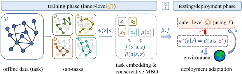
Figure 2: Overview of DROP. Given offline dataset $\mathcal{D}$, we decompose the data into $N$ ($=4$ in the diagram) subsets $\mathcal{D}_{\left[N\right]}$. Over the decomposed sub-tasks, we learn a task embedding $\phi(\mathbf{z}|n)$ and conduct conservative MBO by learning a score model $f(\mathbf{s},\mathbf{a},\mathbf{z})$ and $N$ behavior policies (modeled by a contextual policy $\beta(\mathbf{a}|\mathbf{s},\mathbf{z})$). During test-time, at state $\mathbf{s}$, we perform test-time adaptation by adapting the policy (contextual variable) with $\pi^{*}(\mathbf{a}|\mathbf{s})=\beta\left(\mathbf{a}|\mathbf{s},\mathbf{z}^{*}\right)$, where $\mathbf{z}^{*}=\arg\max_{\mathbf{z}}f(\mathbf{s},\beta(\mathbf{a}|\mathbf{s},\mathbf{z}),\mathbf{z})$.

We present our framework in Figure 2. In Sections 3.1 and 3.2, we will answer questions $\mathtt{Q1}$ and $\mathtt{Q2}$, setting a learned MBO score model as "" ($\mathtt{A1}$) and introducing a conservative regularization over the score model ($\mathtt{A2}$). In Section 3.3, we will answer $\mathtt{Q3}$, where we show that conducting outer-level optimization during testing can produce an adaptive embedding inference across states ($\mathtt{A3}$).

3.1 Task Decomposition

Our core idea is to explore MBO in the non-iterative bi-level offline RL framework (Figure 1 right), while capturing the sequential characteristics of RL tasks and answering the raised questions ($\mathtt{Q1}$, $\mathtt{Q2}$, and $\mathtt{Q3}$). To begin with, we first decompose the offline data $\mathcal{D}$ into $N$ offline subsets $\mathcal{D}_{[N]}:=\{\mathcal{D}_{1},\dots,\mathcal{D}_{N}\}$. In other words, we decompose an offline task, learning with $\mathcal{D}$, into multiple offline sub-tasks, learning with $\mathcal{D}_{n}\in\mathcal{D}_{[N]}$ respectively. Then, for sub-task $n\in[1,N]$, we can perform behavior cloning (BC) to fit a parametric behavior policy $\beta_{n}:\mathcal{S}\times\mathcal{A}\to[0,1]$ to model the corresponding offline subset $\mathcal{D}_{n}$:

$$\beta_{n}\leftarrow\arg\max_{\beta_{n}}\mathbb{E}_{(\mathbf{s},\mathbf{a})\sim\mathcal{D}_{n}}\big{[}\log\beta_{n}(\mathbf{a}|\mathbf{s})\big{]}.$$ (4)

Additionally, such a decomposition also comes with the benefit that it provides an avenue to exploit the hybrid modes in offline data $\mathcal{D}$, because that $\mathcal{D}$ is often collected using hybrid data-generating behavior policies [18], which suggests that fitting a single behavior policy may not be optimal to model the multiple modes of the offline data distribution (see Appendix A for empirical evidence). In real-world tasks, it is also often the case that offline data exhibit hybrid behaviors. Thus, to encourage the emergence of diverse sub-tasks that capture distinct behavior modes, we perform a simple task decomposition according to the returns of trajectories in $\mathcal{D}$, heuristically ensuring that trajectories in the same sub-task share similar returns and trajectories from different sub-tasks have distinct returns.

3.2 Task Embedding and Conservative MBO

Naive MBO over behavior policies. Benefiting from the above offline task decomposition, we can conduct MBO over a set of input-score ($\mathbf{x},y$) pairs, where we model the (parameters of) behavior policies $\beta_{n}$ as the design input $\mathbf{x}$ and the corresponding expected returns at initial states $J(\beta_{n})$ as the score $y$. Note that, ideally, evaluating behavior policy $\beta_{n}$, i.e., calculating $J(\beta_{n})\equiv\mathbb{E}_{\mathbf{s}_{0}}\left[V^{\beta_{n}}(\mathbf{s}_{0})\right]$, with subset $\mathcal{D}_{n}$ will never trigger the overestimation of values in the inner-level optimization. By introducing a score model $f:\Pi\to\mathbb{R}$ and setting it as the transfer information "" in $\mathtt{Q1}$, we can then perform outer-level policy inference with

$$\pi^{*}(\mathbf{a}|\mathbf{s}) \leftarrow\arg\max_{\pi}\ {f}\left(\pi\right),\text{\ where\ }{f}=\arg\min_{f}\ \mathbb{E}_{n}\left[\big{(}f(\beta_{n})-J(\beta_{n})\big{)}^{2}\right].$$ (5)

However, directly performing optimization-based inference (outer-level optimization), $\max_{\pi}{f}\left(\pi\right)$, will quickly find an invalid input for which the learned score model ${f}$ outputs erroneously large values ($\mathtt{Q2}$). Furthermore, it is particularly severe if we perform the inference directly over the parameters of policy networks, accounting for the fact that the parameters of behavior policies lie on a narrow manifold in a high-dimensional parametric space.

Task embedding. To enable feasible out-level policy inference, we propose to decouple MBO techniques from high-dimensional policy parameters. We achieve this by learning a latent embedding space $\mathcal{Z}$ with an information bottleneck ($\mathrm{dim}(\mathcal{Z})\ll\min(N,\mathrm{dim}({\Pi}))$). As long as the high-dimensional parameters of behavior policies can be inferred from the embedding $\mathbf{z}\in\mathcal{Z}$, we can use $\mathbf{z}$ to represent the corresponding sub-task (or the behavior policy). Formally, we learn a deterministic task embedding $\phi:\mathbb{R}^{N}\to\mathcal{Z}$ and a contextual behavior policy $\beta:\mathcal{S}\times\mathcal{Z}\times\mathcal{A}\to[0,1]$ that replaces $N$ separate behavior policies in Equation 4:

$$\beta(\mathbf{a}|\mathbf{s},\mathbf{z}),\phi(\mathbf{z}|n)\leftarrow\arg\max_{\beta,\phi}\ \mathbb{E}_{\mathcal{D}_{n}\sim\mathcal{D}_{[N]}}\mathbb{E}_{(\mathbf{s},\mathbf{a})\sim\mathcal{D}_{n}}\left[\log\beta(\mathbf{a}|\mathbf{s},\phi(\mathbf{z}|n))\right],$$ (6)

Conservative MBO. In principle, by substituting the learned task embedding $\phi(\mathbf{z}|n)$ and contextual behavior policy $\beta(\mathbf{a}|\mathbf{s},\mathbf{z})$ into Equation 5, we can then conduct MBO over the embedding space: first learning $f:\mathcal{Z}\to\mathbb{R}$ with $\min_{f}\mathbb{E}_{n,\phi(\mathbf{z}|n)}\left[\left(f(\mathbf{z})-J(\beta_{n})\right)^{2}\right]$, and then setting the optimal embedding with $\mathbf{z}^{*}=\arg\max_{\mathbf{z}}{f}(\mathbf{z})$ and the corresponding optimal policy with $\pi^{*}(\mathbf{a}|\mathbf{s})=\beta(\mathbf{a}|\mathbf{s},\mathbf{z}^{*})$. However, we must deliberate a new OOD issue in the $\mathcal{Z}$-space, stemming from the original distribution shift in the parametric space when directly optimizing Equation 5.

Motivated by the energy model [38] and the conservative regularization [35], we introduce a conservative score model objective, additionally regularizing the scores of OOD embeddings $\mu(\mathbf{z})$:

$${f} \leftarrow\arg\min_{f}\ \mathbb{E}_{n,\phi(\mathbf{z}|n)}\left[\big{(}f(\mathbf{z})-J(\beta_{n})\big{)}^{2}\right],\text{\ s.t. \ }\mathbb{E}_{\mu(\mathbf{z})}\left[f(\mathbf{z})\right]-\mathbb{E}_{n,\phi(\mathbf{z}|n)}\left[f(\mathbf{z})\right]\leq\eta,$$ (7)

where we set $\mu(\mathbf{z})$ to be the uniform distribution over $\mathcal{Z}$-space. Intuitively, as long as the scores of OOD embeddings $\mathbb{E}_{\mu(\mathbf{z})}\left[f(\mathbf{z})\right]$ is lower than that of in-distribution embeddings $\mathbb{E}_{n,\phi(\mathbf{z}|n)}\left[f(\mathbf{z})\right]$ (up to a threshold $\eta$), conducting embedding inference with $\mathbf{z}^{*}=\arg\max_{\mathbf{z}}{f}(\mathbf{z})$ would produce the best and confident solution, avoiding towards OOD embeddings that are far away from the training set.

Now we have reframed the non-iterative bi-level offline RL problem as one of offline MBO: in the inner-level optimization ($\mathtt{Q1}$), we set the practical choice for "" as the learned score model $f$ ($\mathtt{A1}$); in the outer-level optimization ($\mathtt{Q2}$), we introduce task embedding and conservative regularization to avoid over-optimistic exploitation when exploiting $f$ for policy/embedding inference ($\mathtt{A2}$). In the next section, we will show how to slightly change the form of the score model $f$, so as to leverage the sequential characteristic (loop in Figure 1) of RL tasks and answer the left $\mathtt{Q3}$.

3.3 Test-time Adaptation

Recalling that we update ${f}(\mathbf{z})$ to regress the value at initial states $\mathbb{E}_{\mathbf{s}_{0}}\left[V^{\beta_{n}}(\mathbf{s}_{0})\right]$ in Equation 7, we then conduct outer-level inference with $\mathbf{z}^{*}=\arg\max_{\mathbf{z}}{f}(\mathbf{z})$ and rollout the $z^{*}$-conditioned policy $\pi^{*}(\mathbf{a}|\mathbf{s}):=\beta(\mathbf{a}|\mathbf{s},\mathbf{z}^{*})$ until the end of testing/deployment rollout episode. In essence, such an inference can produce a confident extrapolation over the distribution of behavior policy embeddings. Going beyond the outer-level policy/embedding inference only at the initial states, we propose that we can benefit from performing inference at any rollout state in deployment ($\mathtt{A3}$).

To enable test-time adaptation, we model the score model with $f:\mathcal{S}\times\mathcal{A}\times\mathcal{Z}\to\mathbb{R}$, taking a state-action as an extra input. Then, we encourage the score model to regress the values of behavior policies over all state-action pairs, $\min_{f}\mathbb{E}_{n,\phi(\mathbf{z}|n)}\mathbb{E}_{(\mathbf{s},\mathbf{a})\sim\mathcal{D}_{n}}\left[\left(f(\mathbf{s},\mathbf{a},\mathbf{z})-Q^{\beta_{n}}(\mathbf{s},\mathbf{a})\right)^{2}\right]$. For simplicity, instead of learning a separate value function $Q^{\beta_{n}}$ for each behavior policy, we learn the score model directly with the TD-error used for learning the value function $Q^{\beta_{n}}(\mathbf{s},\mathbf{a})$ as in Equation 1, together with the conservative regularization in Equation 7:

$${f}\leftarrow\arg\min_{f}\mathbb{E}_{\mathcal{D}_{n}\sim\mathcal{D}_{[N]}}\mathbb{E}_{(\mathbf{s},\mathbf{a},\mathbf{s}^{\prime},\mathbf{a}^{\prime})\sim\mathcal{D}_{n}}\left[\left(R(\mathbf{s},\mathbf{a})+\gamma\bar{f}(\mathbf{s}^{\prime},\mathbf{a}^{\prime},\phi(\mathbf{z}|n))-f(\mathbf{s},\mathbf{a},\phi(\mathbf{z}|n))\right)^{2}\right],$$ (8)

$$\text{\ s.t. \ }\mathbb{E}_{n,\mu(\mathbf{z})}\mathbb{E}_{\mathbf{s}\sim\mathcal{D}_{n},\mathbf{a}\sim\beta(\mathbf{a}|\mathbf{s},\mathbf{z})}\left[f(\mathbf{s},\mathbf{a},\mathbf{z})\right]-\mathbb{E}_{n,\phi(\mathbf{z}|n)}\mathbb{E}_{\mathbf{s}\sim\mathcal{D}_{n},\mathbf{a}\sim\beta(\mathbf{a}|\mathbf{s},\mathbf{z})}\left[f(\mathbf{s},\mathbf{a},\mathbf{z})\right]\leq\eta,$$

where $\bar{f}$ denotes a target network and we update the target $\bar{f}$ with soft updates: $\bar{f}=(1-\upsilon)\bar{f}+\upsilon f$.

In test-time, we thus can dynamically adapt the outer-level optimization, setting the inferred optimal policy $\pi^{*}(\mathbf{a}|\mathbf{s})=\beta(\mathbf{a}|\mathbf{s},\mathbf{z}^{*}(\mathbf{s}))$, where $z^{*}(\mathbf{s})=\arg\max_{z}{f}\big{(}\mathbf{s},\beta(\mathbf{a}|\mathbf{s},\mathbf{z}),\mathbf{z}\big{)}$. Specifically, at any state $\mathbf{s}$ in the test-time, we can perform gradient ascent to find the optimal behavior embedding: $z^{*}(\mathbf{s})=\mathbf{z}^{\circ}_{K}(\mathbf{s}):=\mathrm{GradAscent}(\mathbf{s},\mathbf{z}_{0}^{\circ},K)$, where $\mathbf{z}_{0}^{\circ}$ is the starting point and for $k=0,1\dots,K-1$,

$$\mathbf{z}^{\circ}_{k+1}(\mathbf{s}) \leftarrow\mathbf{z}^{\circ}_{k}(\mathbf{s})+\eta\nabla_{\mathbf{z}}{f}(\mathbf{s},\beta(\mathbf{a}|\mathbf{s},\mathbf{z}),\mathbf{z}))|_{\mathbf{z}=\mathbf{z}^{\circ}_{k}}.$$ (9)

Table 1: Comparison of non-iterative bi-level offline RL methods, where we use $\mathsf{R}(\tau)$ to represent the return of a sampling trajectory $\tau$ and use $\mathsf{R}(\mathbf{s},\mathbf{a})$ to represent the expected return of trajectories starting from $(\mathbf{s},\mathbf{a})$. The checkmark in $\mathtt{A2}$ indicates whether the exploitation to "" is regularized for outer-level optimization and that in $\mathtt{A3}$ indicates whether test-time adaptation is supported.

	Inner-level	Outer-level	"" in $\mathtt{A1}$	$\mathtt{A2}$	$\mathtt{A3}$
F-BC	BC over filtered $\tau$ with high $\mathsf{R}(\tau)$	—	$\pi(\mathbf{a}|\mathbf{s})$	✗	✗
RvS-R [14]	$\min_{\pi}-\mathbb{E}\left[\log\pi(\mathbf{a}|\mathbf{s},\mathsf{R}(\tau))\right]$	handcraft $\mathsf{R}_{\text{target}}$	$\pi(\mathbf{a}|\mathbf{s},\cdot)$	✗	✗
Onestep [6]	$\min_{Q}\mathcal{L}(Q(\mathbf{s},\mathbf{a}),\mathsf{R}(\mathbf{s},\mathbf{a}))$	$\arg\max_{{\color[rgb]{0,0,1}\mathbf{a}}}Q_{\beta}(\mathbf{s},\beta(\mathbf{a}|\mathbf{s}))$	$Q_{\beta}(\mathbf{s},\mathbf{a})$	✗	✔
COMs [62]	$\min_{f}\mathcal{L}(f(\beta_{\tau}),\mathsf{R}(\tau))$	$\arg\max_{{\color[rgb]{0,0,1}\beta}}f(\beta)$	$f(\beta)$	✔	✗
DROP (ours)	$\min_{f}\mathcal{L}(f(\mathbf{s},\mathbf{a},\mathbf{z}),\mathsf{R}(\mathbf{s},\mathbf{a},\mathbf{z}))$	$\arg\max_{{\color[rgb]{0,0,1}\mathbf{z}}}f(\mathbf{s},\beta(\mathbf{a}|\mathbf{z}),\mathbf{z})$	$f(\mathbf{s},\mathbf{a},\mathbf{z})$	✔	✔

3.4 Connection to Prior Non-iterative Offline Methods

In Table 1, we summarize the comparison with prior representative non-iterative offline RL methods. Intuitively, our DROP (using returns to decompose $\mathcal{D}$) is similar in spirit to F-BC and RvS-R [14], both of which use return $\mathsf{R}(\tau)$ to guide the inner-level optimization. However, both F-BC and RvS-R leave $\mathtt{Q2}$ unanswered. In outer-level, F-BC can not enable policy extrapolation, which heavily relies on the data quality in offline tasks. RvS-R needs to handcraft a target return (as the contextual variable for $\pi(\mathbf{a}|\mathbf{s},\cdot)$), which also probably triggers the potential distribution mismatch between the hand-crafted contextual variable (i.e., the desired return) and the actual rollout return induced by the learned policy when conditioning on the given contextual variable.

Diving deeper into the bi-level optimization, we can also find DROP combines the advantages of Onestep [6] and COMs [62], where Onestep answers $\mathtt{Q3}$  and performs outer-level optimization in action space ($\arg\max_{{\color[rgb]{0,0,1}\mathbf{a}}}$), COMs answers $\mathtt{Q2}$ and performs that in parameter space ($\arg\max_{{\color[rgb]{0,0,1}\beta}}$), while our DROP answers both $\mathtt{Q2}$ and $\mathtt{Q3}$ and performs that in embedding space ($\arg\max_{{\color[rgb]{0,0,1}\mathbf{z}}}$). Specifically, DROP thus allows us to ($\mathtt{A2}$) conduct safe extrapolation in outer-level and ($\mathtt{A3}$) perform test-time adaptation in testing rather than simply conducting outer-level optimization at initial states as in COMs.

3.5 Practical Implementation

Algorithm 1 DROP (Training)

Require: Dataset of trajectories: $\mathcal{D}=\{\tau\}$.

1:  Decompose $\mathcal{D}$ into $N$ sub-sets $\mathcal{D}_{[N]}$.

2:  Initialize $\phi(\mathbf{z}|n)$, $\beta(\mathbf{a}|\mathbf{s},\mathbf{z})$, and $f(\mathbf{s},\mathbf{a},\mathbf{z})$.

3:  while not converged do

4:     Sample a sub-task: $\mathcal{D}_{n}\sim\mathcal{D}_{[N]}$.

5:     Learn $\phi$, $\beta$, and $f$ with Equations 6 and 8.

6:  end while

Return: $\beta(\mathbf{a}|\mathbf{s},\mathbf{z})$ and $f(\mathbf{s},\mathbf{a},\mathbf{z})$.

Algorithm 2 DROP (Testing/Deployment)

Require: Env, $\beta(\mathbf{a}|\mathbf{s},\mathbf{z})$, and $f(\mathbf{s},\mathbf{a},\mathbf{z})$.

1:  $\mathbf{s}_{0}$ = Env.Reset().

2:  while not done do

3:     Test-time adaptation: $\mathbf{z}^{*}(\mathbf{s}_{t})=\arg\max_{\mathbf{z}}f(\mathbf{s}_{t},\beta(\mathbf{a}_{t}|\mathbf{s}_{t},\mathbf{z}),\mathbf{z})$.

4:     Sample action: $\mathbf{a}_{t}\sim\beta(\mathbf{a}_{t}|\mathbf{s}_{t},\mathbf{z}^{*}(\mathbf{s}_{t}))$.

5:     Step Env: $\mathbf{s}_{t+1}\sim P(\mathbf{s}_{t+1}|\mathbf{s}_{t},\mathbf{a}_{t})$.

6:  end while

We now summarize the DROP algorithm (see Algorithm 1 for the training phase and Algorithm 2 for the testing phase). During training (inner-level optimization), we alternate between updating $\phi(\mathbf{z}|n)$, $\beta(\mathbf{a}|\mathbf{s},\mathbf{z})$, and $f(\mathbf{s},\mathbf{a},\mathbf{z})$, wherein we update $\phi$ with both maximum likelihood loss and TD-error loss in Equations 6 and 8. During testing (outer-level optimization), we use the gradient ascent as specified in Equation 9 to infer the optimal embedding $z^{*}$. Instead of simply sampling a single starting point $\mathbf{z}_{0}^{\circ}$, we choose $N$ starting points corresponding to all the embeddings $\{\mathbf{z}_{n}\}$ of sub-tasks, and then choose the optimal $\mathbf{z}^{*}(\mathbf{s})$ from those updated embeddings for which the learned $f$ outputs the highest score, i.e., $\mathbf{z}^{*}(\mathbf{s})=\arg\max_{\mathbf{z}}\ f(\mathbf{s},\beta(\mathbf{a}|\mathbf{s},\mathbf{z}),\mathbf{z})$ s.t. $\mathbf{z}\in\{\mathrm{GradAscent}(\mathbf{s},\mathbf{z}_{n},K)|n=1,\dots,N\}$. Then, we sample action from $\pi^{*}(\mathbf{a}|\mathbf{s}):=\beta(\mathbf{a}|\mathbf{s},\mathbf{z}^{*}(\mathbf{s}))$.

4 Related Work

Offline RL. In offline RL, learning with offline data is prone to exploiting OOD state-actions and producing over-estimated values, which makes vanilla iterative policy/value optimization challenging. To eliminate the problem, a number of methods have been explored, in essence, by either introducing a policy/value regularization in the iterative loop or trying to eliminate the iterative loop itself.

Iterative methods: Sticking with the normal iterative updates in RL, offline policy regularization methods aim to keep the learning policy to be close to the behavior policy under a probabilistic distance [8, 19, 30, 33, 45, 46, 52, 54, 58, 67, 73]. Some works also conduct implicit policy regularization with variants of importance sampling [39, 47, 51]. Besides regularizing policy, it is also feasible to constrain the substitute value function in the iterative loop. Methods constraining the value function aim at mitigating the over-estimation, which typically introduces pessimism to the prediction of the Q-values [9, 27, 35, 41, 48, 49] or penalizes the value with an uncertainty quantification [3, 5, 56, 68], making the value for OOD state-actions more conservative. Similarly, another branch of model-based methods [29, 71, 72, 57] also perform iterative bi-level updates, alternating between regularized evaluation and improvement. Different from this iterative paradigm, DROP only evaluates values of behavior policies in the inner-level optimization, avoiding the potential overestimation for values of learning policies and eliminating error propagation between two levels.

Non-iterative methods: Another complementary line of work studies how to eliminate the iterative updates, which simply casts RL as a weighted or conditional imitation learning problem ($\mathtt{Q1}$). Derived from the behavior-regularization RL [22, 64], the former conducts weighted behavior cloning: first learning a value function for the behavior policy, then weighing the state-action pairs with the learned values or advantages [1, 12, 66, 54]. Besides, some works propose an implicit behavior policy regularization that similarly does not estimate values of new learning policies: initializing the learning policy with a behavior policy [50] or performing only a "one-step" update (policy improvement) over the behavior policy [20, 24, 75]. For the latter, this branch method typically builds upon the hindsight information matching [4, 15, 28, 36, 44, 43, 55, 65], assuming that the future trajectory information can be useful to infer the middle decision that leads to the future and thus relabeling the trajectory with the reached states or returns. Due to the simplicity and stability, RvS-based methods advocate for learning a goal-conditioned or reward-conditioned policy with supervised regression [10, 13, 14, 21, 25, 42, 60, 69]. However, these works do not fully exploit the non-iterative framework and fail to answer the raised questions, which either does not regularize the inner-level optimization when exploiting "" in outer-level ($\mathtt{Q2}$), or does not support test-time adaptation ($\mathtt{Q3}$).

Offline MBO. Similar to offline RL, the main challenge of MBO is to reason about uncertainty and OOD values [7, 16], since a direct gradient-ascent against the learned score model can easily produce invalid inputs that are falsely and highly scored. To counteract the effect of model exploitation, prior works introduce various techniques, including normalized maximum likelihood estimation [17], model inversion networks [32], local smoothness prior [70], and conservative objective models (COMs) [62]. Compared to COMs, DROP shares similarities with the conservative model, but instantiates on the embedding space instead of the parameter space. Such difference is nontrivial, not only because DROP avoids the adversarial optimization employed in COMs, but also because DROP allows test-time adaptation, enabling dynamical inference across states at testing.

5 Experiments

In this section, we present our empirical results. We first give examples to illustrate the test-time adaptation. Then we evaluate DROP against prior offline RL algorithms on the D4RL benchmark. Finally, we provide the computation cost regarding the test-time adaptation protocol. For more offline-to-online fine-tuning results, ablation studies w.r.t. the decomposition rules and the conservative regularization, and training details on the hyper-parameters, we refer the readers to the appendix.

Illustration of test-time adaptation. To better understand the test-time adaptation of DROP, we include four comparisons that exhibit different embedding inference rules at testing/deployment:

(1) DROP-Best: At initial state $\mathbf{s}_{0}$, we choose the best embedding from those embeddings of behavior policies, ${\color[rgb]{0,0,0}\mathbf{z}^{*}_{0}(\mathbf{s}_{0})}=\arg\max_{z}{f}(\mathbf{s}_{0},\beta(\mathbf{a}_{0}|\mathbf{s}_{0},\mathbf{z}),\mathbf{z})$ s.t. $\mathbf{z}\in\mathbf{z}_{[N]}:=\{\mathbf{z}_{1},\dots,\mathbf{z}_{N}\}$, and keep this embedding fixed for the entire episode, i.e., setting $\pi^{*}(\mathbf{a}_{t}|\mathbf{s}_{t})=\beta(\mathbf{a}_{t}|\mathbf{s}_{t},{\color[rgb]{0,0,0}\mathbf{z}^{*}_{0}(\mathbf{s}_{0})})$.

(2) DROP-Grad: At initial state $\mathbf{s}_{0}$, we conduct inference (gradient ascent on starting point $\mathbf{z}^{*}_{0}(\mathbf{s}_{0})$) with ${\color[rgb]{0,0,0}\mathbf{z}^{*}(\mathbf{s}_{0})}=\arg\max_{z}{f}(\mathbf{s}_{0},\beta(\mathbf{a}_{0}|\mathbf{s}_{0},\mathbf{z}),\mathbf{z})$, and keep ${\color[rgb]{0,0,0}\mathbf{z}^{*}(\mathbf{s}_{0})}$ fixed throughout the test rollout.

(3) DROP-Best-Ada: We adapt the policy by setting $\pi^{*}(\mathbf{a}_{t}|\mathbf{s}_{t})=\beta(\mathbf{a}_{t}|\mathbf{s}_{t},{\color[rgb]{0,0,0}\mathbf{z}^{*}_{0}(\mathbf{s}_{t})})$, where we choose the best embedding $\mathbf{z}^{*}_{0}(\mathbf{s}_{t})$ directly from those embeddings of behavior policies for which the score model outputs the highest score, i.e., ${\color[rgb]{0,0,0}\mathbf{z}^{*}_{0}(\mathbf{s}_{t})}=\arg\max_{\mathbf{z}}f(\mathbf{s}_{t},\beta(\mathbf{a}_{t}|\mathbf{s}_{t},\mathbf{z}),\mathbf{z})$ s.t. $\mathbf{z}\in\mathbf{z}_{[N]}$.

(4) DROP-Grad-Ada (as described in Section 3.5): We set $\pi^{*}(\mathbf{a}_{t}|\mathbf{s}_{t})$$=\beta(\mathbf{a}_{t}|\mathbf{s}_{t},{\color[rgb]{0,0,0}\mathbf{z}^{*}(\mathbf{s}_{t})})$ and choose the best embedding ${\color[rgb]{0,0,0}\mathbf{z}^{*}(\mathbf{s}_{t})}$ from those updated embeddings of behavior policies, i.e., ${\color[rgb]{0,0,0}\mathbf{z}^{*}(\mathbf{s}_{t})}=\arg\max_{\mathbf{z}}f(\mathbf{s}_{t},\beta(\mathbf{a}_{t}|\mathbf{s}_{t},\mathbf{z}),\mathbf{z})$ s.t. $\mathbf{z}\in\{\mathrm{GradAscent}(\mathbf{s}_{t},\mathbf{z}_{n},K)|n=1,\dots,N\}$.

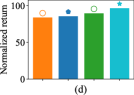
Figure 3: Visualization of the embedding inference (a, b, c1, c2) and performance comparison (d). $\mathbf{z}_{[N]}$ denotes embeddings of all behavior policies. $\mathbf{z}^{*}_{0}(\mathbf{s}_{0})$, $\mathbf{z}^{*}(\mathbf{s}_{0})$, $\mathbf{z}^{*}_{0}(\mathbf{s}_{t})$, and $\mathbf{z}^{*}(\mathbf{s}_{t})$ denote the selected embeddings in DROP- Best, Grad, Best-Ada, and Grad-Ada implementations respectively.

In Figure 3, we visualize the four different inference rules and report the corresponding performance in the halfcheetah-medium-expert task [18]. In Figure 3 (a), we set the starting point as the best embedding $\mathbf{z}^{*}_{0}(\mathbf{s}_{0})$ in $\mathbf{z}_{[N]}$, and perform gradient ascent to find the optimal $\mathbf{z}^{*}_{0}(\mathbf{s}_{0})$ for DROP-Grad. In Figure 3 (b), we can find that at different time steps, DROP-Best-Ada chooses different embeddings for $\beta(\mathbf{a}_{t}|\mathbf{s}_{t},\cdot)$. Intuitively, performing such a dynamical embedding inference enables us to combine different embeddings, thus stitching behavior policies at different states. Further, in Figure 3 (c1, c2), we find that performing additional inference (with gradient ascent) in DROP-Grad-Ada allows to extrapolate beyond the embeddings of behavior policies, and thus results in sequential composition of new embeddings (policies) across different states. For practical impacts of these different inference rules, we provide the performance comparison in Figure 3 (d), where we can find that performing gradient-based optimization (*-Grad-*) outperforms the natural selection among those embeddings of behavior policies/sub-tasks (*-Best-*), and rollout with adaptive embedding inference (DROP-*-Ada) outperforms that with fixed embeddings (DROP-Best and DROP-Grad). In subsequent experiments, if not explicitly stated, DROP takes the DROP-Grad-Ada implementation by default.

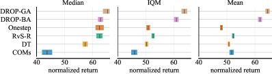
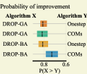
Figure 4: (Left) Aggregate metrics [2] on 12 D4RL tasks. Higher median, IQM, and mean scores are better. (Right) Each row shows the probability of improvement that the algorithm X on the left outperforms algorithm Y on the right. The CIs are estimated using the percentile bootstrap (95%) with stratified sampling. For all results of our method, we average the normalized returns across 5 seeds; for each seed, we run 10 evaluation episodes. (GA: Grad-Ada. BA: Best-Ada.)

Empirical performance on benchmark tasks. We evaluate DROP on a number of tasks from the D4RL dataset and make comparisons with prior non-iterative offline RL counterparts.

As suggested by Agarwal et al. [2], we provide the aggregate comparison results to account for the statistical uncertainty. In Figure 4, we report the median, IQM [2], and mean scores of DROP and prior non-iterative offline baselines in 12 D4RL tasks (see individual comparison results in Appendix C). We can find our DROP (Best-Ada and Grad-Ada) consistently outperforms prior non-iterative baselines in both median, IQM, and mean metrics. Compared to the most related baseline Onestep and COMs (see Table 1), we provide the probability of performance improvement in Figure 4 right. We can find that DROP-Grad-Ada shows a robust performance improvement over Onestep and COMs, with an average improvement probability of more than 80%.

Comparison with latent policy methods. Note that one additional merit of DROP is that it naturally accounts for hybrid modes in $\mathcal{D}$ by conducting task decomposition in inner-level, we thus compare DROP to latent policy methods (PLAS [74] and LAPO [11]) that use conditional variational autoencoder (CVAE) to model offline data and also account for multi-modes in offline data. Essentially, both our DROP and baselines (PLAS and LAPO) learn a latent policy in the inner-level optimization, except that we adopt the non-iterative bi-level learning while baselines are instantiated under the iterative paradigm. By answering $\mathtt{Q3}$, DROP permits test-time adaptation, enabling us to dynamically stitch "skills"(latent behaviors/embeddings as shown in Figure 3) and thus encouraging high-level abstract exploitation in testing. However, the aim of introducing the latent policy in PLAS and LAPO is to regularize the inner-level optimization, which fairly answers $\mathtt{Q2}$ in the iterative offline counterpart but can not provide the potential benefit (test-time adaptation) by answering $\mathtt{Q3}$.

Table 2: Comparison in AntMaze and Gym-MuJoCo domains (v2). Results are averaged over 5 seeds; for each seed, we run 10 evaluation episodes. u: umaze (antmaze). um: umaze-medium. ul: umaze-large. p: play. d: diverse. wa: walker2d. ho: hopper. ha: halfcheetah. r: random. m: medium.

	u	u-d	um-p	um-d	ul-p	ul-d	wa-r	ho-r	ha-r	wa-m	ho-m	ha-m	mean
CQL	74.0	84.0	61.2	53.7	15.8	14.9	-0.2	8.3	22.2	82.1	71.6	49.8	44.8
IQL	87.5	62.2	71.2	70.0	39.6	47.5	5.4	7.9	13.1	77.9	65.8	47.8	49.7
PLAS	70.7	45.3	16.0	0.7	0.7	0.3	9.2	6.7	26.5	75.5	51.0	44.5	28.9
LAPO	86.5	80.6	68.5	79.2	48.8	64.8	1.3	23.5	30.6	80.8	51.6	46.0	55.2
DROP	90.5	92.2	74.1	82.9	57.2	63.3	5.2	20.8	32.0	82.1	74.9	52.4	60.6
DROP std	$\pm 2.4$	$\pm 1.7$	$\pm 3.9$	$\pm 3.5$	$\pm 5.5$	$\pm 2.4$	$\pm 1.6$	$\pm 0.3$	$\pm 2.5$	$\pm 5.2$	$\pm 2.8$	$\pm 2.2$

Note in our naive DROP implementation, we heuristically use the return to conduct task decomposition (motivated by RvS-R), while PLAS and LAPO take each trajectory as a sub-task and use CVAE to learn the latent policy. For a fair comparison, here we also adopt CVAE to model the offline data and afterward take the learned latent embedding in CVAE as the embedding of behaviors, instead of conducting return-guided task decomposition. We provide implementation details (DROP+CVAE) in Appendix A.4 and the comparison results in Table 2 (taking DROP-Grad-Ada implementation). We can observe that our DROP consistently achieves better performance than PLAS in all tasks, and performs better or comparably to LAPO in 10 out of 12 tasks. Additionally, we also provide the results of CQL and IQL [31]. We can find that DROP also leads to significant improvement in performance, consistently demonstrating the competitive performance of DROP against state-of-the-art offline iterative/non-iterative baselines.

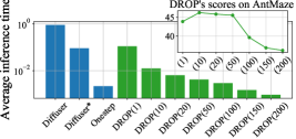
Figure 5: Computation cost across different models and DROP implementations with varying inference time intervals. The number in parenthesis denotes the inference time intervals. In top-right, we also provide the average performance of DROP on AntMaze tasks when using different inference time intervals. (Diffuser* denotes the warm-start implementation of Diffuser.)

Computation cost. One limitation of DROP is that conducting test-time adaptation at each state is usually expensive for inference time. To reduce the computation cost, we find that we can resample (infer) the best embedding $\mathbf{z}^{*}$ after a certain time interval, i.e., $\mathbf{z}^{*}$ does not necessarily need to be updated at each testing state. In Figure 5, we plot the average inference time versus different models and DROP implementations with varying inference time intervals. We see that compared to Diffuser (one offline RL method that also supports test-time adaptation, see quantitative performance comparison in Table 4) [26], DROP can achieve significantly lower computation costs. In Figure 5 top-right, we also illustrate the trade-off between performance and runtime budget as we vary the inference time intervals. We find that by choosing a suitable time interval, we can reduce the inference cost with only a modest drop in performance: DROP(50) brings less computational burden while providing stable performance.

Table 3: Comparison to "distilled" DROP (D-DROP), using Grad-Ada and CVAE implementation.

wa-r ho-r ha-r wa-m ho-m ha-m CQL -0.2 8.3 22.2 82.1 71.6 49.8 IQL 5.4 7.9 13.1 77.9 65.8 47.8 D-DROP 4.5 18.9 27.8 84.2 67.1 50.9 DROP 5.2 20.8 32.0 82.1 74.9 52.4

Comparison to a "distilled" DROP implementation. Our answer to $\mathtt{Q3}$ is that we conduct outer-level optimization in the testing phase. Similarly, we can design a "distilled" DROP implementation: we keep the same treatment as DROP for $\mathtt{Q1}$and $\mathtt{Q2}$, but we perform outer-level optimization on the existing offline data instead of on the testing states, i.e., conducting optimization in $\mathbf{z}$-space for all states in the dataset. Then, we can "distill" the resulting contextual policy and the inferred $\mathbf{z}^{*}$ into a fixed rollout policy. As shown in Table 3, we can see that such a "distilled" DROP implementation achieves competitive performance, approaching DROP’s overall score and slightly outperforming CQL and IQL, which further supports the superiority afforded by the non-iterative offline RL paradigm versus the iterative one.

Table 4: Comparison to adaptive baselines (APE-V and Diffuser). DROP uses Grad-Ada and CVAE implementation.

wa-mr ho-mr ha-mr wa-me ho-me ha-me APE-V 82.9 98.5 64.6 110.0 105.7 101.4 Diffuser 70.6 93.6 37.7 106.9 103.3 88.9 DROP 83.5 96.3 50.9 109.3 107.2 102.2

Comparison to adaptive baselines. One merit of DROP resides in its test-time adaptation ability across rollout states. Thus, here we compare DROP with two offline RL methods that also support test-time adaptation: 1) APE-V [23] learns an uncertainty-adaptive policy and dynamically updates a contextual belief vector at test states, and 2) Diffuser [26] employs a score/return function to guide the diffusion denoising process, i.e., score-guided action sampling. As shown in Table 4, we can see that in medium-replay (mr) and medium-expert (me) domains (v2), DROP can achieve comparable results to APE-V, with a clear improvement over Diffuser.

6 Discussion

In this work, we introduce non-iterative bi-level offline RL, and based on this paradigm, we raise three questions ($\mathtt{Q1}$, $\mathtt{Q2}$, and $\mathtt{Q3}$). To answer that, we reframe the offline RL problem as one of MBO and learn a score model ($\mathtt{A1}$), introduce embedding learning and conservative regularization ($\mathtt{A2}$), and propose test-time adaptation in testing ($\mathtt{A3}$). We evaluate DROP on various tasks, showing that DROP gains comparable or better performance compared to prior methods.

Limitations. DROP also has several limitations. First, the offline data decomposition dominates the following bi-level optimization, and thus choosing a suitable decomposition rule is a crucial requirement for policy inference (see experimental analysis in Appendix A.2). An exciting direction for future work is to study generalized task decomposition rules (e.g., our DROP+CVAE implementation). Second, we find that when the number of sub-tasks is too large, the inference is unstable, where adjacent checkpoint models exhibit larger variance in performance (such instability also exists in prior offline RL methods, discovered by Fujimoto and Gu [19]). One natural approach to this instability is conducting online fine-tuning (see Appendix A.3 for our empirical studies).

Going forward, we believe our work suggests a feasible alternative for generalizable offline robotic learning: by decomposing a single robotic dataset into multiple subsets, offline policy inference can benefit from performing MBO and the test-time adaptation protocol.

Appendix

Appendix A More Experiments

A.1 Single Behavior Policy v.s. Multiple Behavior Policies

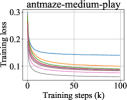
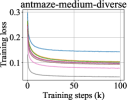
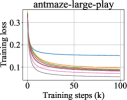
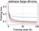
Figure 6: Learning curves of behavior cloning on AntMaze suites (*-v2) in D4RL, where the x-axis denotes the training steps, and the y-axis denotes the training loss. The number $N$ in the legend denotes the number of sub-tasks. If $N=1$, we learn a single behavior policy for the whole offline dataset.

In Figure 6, we provide empirical evidence that learning a single behavior policy (using BC) is not sufficient to characterize the whole offline dataset, and multiple behavior policies (conducting task decomposition) deliver better resilience to characterize the offline data than a single behavior policy.

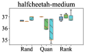
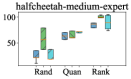
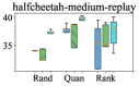
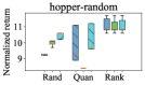
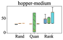
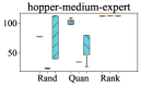
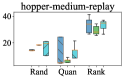
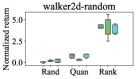
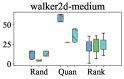
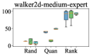
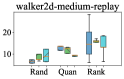
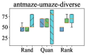
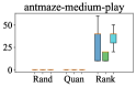
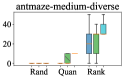
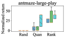
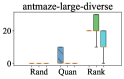
Figure 7: Comparison of three different decomposition rules on D4RL MuJoCo-Gym suite (*-v0) and AntMaze suite (*-v2), where "Rand", "Quan" and "Rank" denote the Random, Quantization, and Rank decomposition rules respectively. We can find across 18 tasks (AntMaze and MuJoCo-Gym suites) and 3 embedding inference methods (DROP-Grad, DROP-Best-Ada, and DROP-Grad-Ada), Rank is more stable and yields better performance compared with the other two decomposition rules.

A.2 Decomposition Rules

In DROP algorithm, we explicitly decompose an offline task into multiple sub-tasks, over which we then reframe the offline policy learning problem as one of offline model-based optimization. In this section, we discuss three different designs for the task decomposition rule.

Random$(N,M)$: We decomposition offline dataset $\mathcal{D}:=\{\tau\}$ into $N$ subsets, each of which contains at most $M$ trajectories that are randomly sampled from the offline dataset.

Quantization$(N,M)$: Leveraging the returns of trajectories in offline data, we first quantize offline trajectories into $N$ bins, and then randomly sample at most $M$ trajectories (as a sub-task) from each bin. Specifically, in the $i$-th bin, the quantized trajectories $\{\tau_{i}\}$ satisfy $\mathrm{R}_{\text{min}}+\Delta*i<\mathrm{Return}(\tau_{i})\leq\mathrm{R}_{\text{min}}+\Delta*(i+1)$, where $\Delta=\frac{(\mathrm{R}_{\text{max}}-\mathrm{R}_{\text{min}})}{N}$, $\mathrm{Return}(\tau_{i})$ denotes the return of trajectory $\tau_{i}$, and $\mathrm{R}_{\text{max}}$ and $\mathrm{R}_{\text{min}}$ denote the maximum and minimum trajectory returns in the offline dataset respectively.

Rank$(N,M)$: We first rank the offline trajectories descendingly based on their returns, and then sequentially sample $M$ trajectories for each subset. (We adopt this decomposition rule in main paper.)

In Figure 7, we provide the comparison of the above three decomposition rules (see the selected number of sub-tasks and the number of trajectories in each sub-task in Table 9). We can find that across a variety of tasks, the decomposition rule has a fundamental impact on the subsequent model-based optimization. Across different tasks and different embedding inference rules, Random and Quantization decomposition rules tend to exhibit large performance fluctuations, which reveals the importance of choosing a suitable task decomposition rule. In our paper, we adopt the Rank decomposition rule, as it demonstrates a more robust performance shown in Figure 7. In Appendix A.4, we adopt the conditional variational auto-encoder (CVAE) to conduct automatic task decomposition (treating each trajectory in offline dataset as an individual task) and we find such implementation (DROP+CVAE) can further improve DROP’s performance. In future work, we also encourage better decomposition rules to decompose offline tasks so as to enable more effective model-based optimization for offline RL tasks.

Comparison with filtered behavior cloning.

We also note that the Rank decomposition rule leverages more high-quality (high-return) trajectories than the other two decomposition rules (Random and Quantization). Thus, a natural question to ask is, is the performance of Rank better than that of Random and Quantization due to the presence of more high-quality trajectories in the decomposed sub-tasks? That is, whether DROP (using the Rank decomposition rule) only conducts behavioral cloning over those high-quality trajectories, thus leading to better performance.

To answer the above question, we compare DROP (using the Rank decomposition rule) with filtered behavior cloning (F-BC), where the latter (F-BC) performs behavior cloning after filtering for trajectories with high returns. We provide the comparison results in Table 5. We can find that in AntMaze tasks, the overall performance of DROP is higher than that of F-BC. For the MuJoCo-Gym suite, DROP-based methods outperform F-BC on these offline tasks that contain plenty of sub-optimal trajectories, including the random, medium, and medium-replay domains. This result indicates that DROP can leverage embedding inference (extrapolation) to find a better policy beyond all the behavior policies in sub-tasks, which is more effective than simply performing imitation learning on a subset of the dataset.

Table 5: Comparison between our DROP (using the Rank decomposition rule) and filtered behavior cloning (F-BC) on D4RL AntMaze and MuJoCo suites (*-v2). We take the baseline results of BC and F-BC from Emmons et al. [14], where F-BC is trained over the top $10\%$ trajectories, ordered by the returns. Our DROP results are computed over 5 seeds and 10 episodes for each seed.

Tasks		BC	F-BC	DROP-Grad	DROP-Best-Ada	DROP-Grad-Ada
antmaze-umaze		54.6	60	72 $\pm$ 17.2	78 $\pm$ 11.7	80 $\pm$ 12.6
antmaze-umaze-diverse		45.6	46.5	48 $\pm$ 22.3	62 $\pm$ 16	66 $\pm$ 12
antmaze-medium-play		0	42.1	24 $\pm$ 10.2	34 $\pm$ 12	30 $\pm$ 21
antmaze-medium-diverse		0	37.2	20 $\pm$ 19	24 $\pm$ 12	30 $\pm$ 16.7
antmaze-large-play-		0	28	24 $\pm$ 8	36 $\pm$ 17.4	42 $\pm$ 17.2
antmaze-large-diverse		0	34.3	14 $\pm$ 8	20 $\pm$ 14.1	26 $\pm$ 13.6
halfcheetah	random	2.3	2	2.3 $\pm$ 0	2.3 $\pm$ 0	2.3 $\pm$ 0
hopper	random	4.8	4.1	5.1 $\pm$ 0.8	5.4 $\pm$ 0.7	5.5 $\pm$ 0.6
walker2d	random	1.7	1.7	2.8 $\pm$ 1.7	3 $\pm$ 1.6	3 $\pm$ 1.8
halfcheetah	medium	42.6	42.5	42.4 $\pm$ 0.7	42.9 $\pm$ 0.4	43.1 $\pm$ 0.4
hopper	medium	52.9	56.9	57.5 $\pm$ 6.4	60.3 $\pm$ 6.1	59.5 $\pm$ 5.1
walker2d	medium	75.3	75	76.5 $\pm$ 2.4	75.8 $\pm$ 3	79.1 $\pm$ 1.4
halfcheetah	medium-replay	36.6	40.6	39.5 $\pm$ 1	40.4 $\pm$ 0.8	40.3 $\pm$ 1.2
hopper	medium-replay	18.1	75.9	48 $\pm$ 17.7	83.4 $\pm$ 6.5	87.4 $\pm$ 2.1
walker2d	medium-replay	26	62.5	37.4 $\pm$ 13.5	60.9 $\pm$ 7.4	61.9 $\pm$ 2.3

A.3 Online Fine-tuning

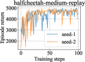
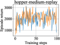
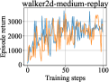
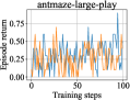
Figure 8: Learning curves of DROP, where the x-axis denotes the training steps (k), the y-axis denotes the evaluation return (using DROP-Best embedding inference rule). We only show two seeds for legibility.

Online fine-tuning (checkpoint-level).

In Figure 8, we show the learning curves of DROP-Best on four DR4L tasks. We can find that DROP exhibits a high variance (in performance) across training steps, which means the performance of the agent may be dependent on the specific stopping point chosen for evaluation (such instability also exists in prior offline RL methods, Fujimoto and Gu [19]).

To choose a suitable stopping checkpoint over which we perform the DROP inference (DROP-Grad, DROP-Best-Ada and DROP-Grad-Ada), we propose to conduct checkpoint-level online fine-tuning (see Algorithm 3 in Section B for more details): we evaluate each of the latest $T$ checkpoint models and choose the best one that leads to the highest episode return.

In Figure 9, we show the total normalized returns across all the tasks in each suite (including Maze2d, AntMaze, and MuJoCo-Gym). We can find that in most tasks, fine-tuning (FT) can guarantee performance improvement. However, we also find such fine-tuning causes negative impacts on performance in AntMaze(*-v0) suite. The main reason is that, in this checkpoint-level fine-tuning, we choose the "suitable" checkpoint model using the DROP-Best embedding inference rule, while we adopt the other three embedding inference rules (DROP-Grad, DROP-Best-Ada and DROP-Grad-Ada) at the test time. Such a finding also implies that the success of DROP’s test-time adaptation is not entirely dependent on the best embedding across sub-tasks (i.e., the best embedding ${\color[rgb]{0,0,0}\mathbf{z}^{*}_{0}(\mathbf{s}_{0})}$ in DROP-Best), but requires switching between some "suboptimal" embeddings (using DROP-Best-Ada) or extrapolating new embeddings (using DROP-Grad-Ada).

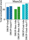
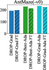
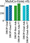
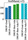
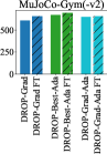
Figure 9: Total normalized returns across all the tasks in Maze2d, AntMaze, and MuJoCo-Gym suites.

Online fine-tuning (embedding-level).

Beyond the above checkpoint-level fine-tuning procedure, we can also conduct embedding-level online fine-tuning: we aim to choose a suitable gradient update step for the gradient-based embedding inference rules (including DROP-Grad and DROP-Grad-Ada). Similar to the checkpoint-level fine-tuning, we first conduct the test-time adaptation procedure (DROP-Grad and DROP-Grad-Ada) over a set of gradient update steps, and then choose the best step that leads to the highest episode return (see Algorithm 4 in Section B for more details).

In Table 6, we compare our DROP (DROP-Grad and DROP-Grad-Ada) to three offline RL methods (AWAC [53], CQL [35] and IQL [31]), reporting the initial performance and the performance after online fine-tuning. We can find that the embedding-level fine-tuning (0.3M) enables a significant improvement in performance. The fine-tuned DROP-Grad-Ada (0.3M) outperforms the AWAC and CQL counterparts in most tasks, even though we take fewer rollout steps to conduct the online fine-tuning (baselines take $1$M online rollout steps, while DROP-based fine-tuning takes $0.3$M steps). However, there is still a big gap between the fine-tuned IQL and the embedding-level fine-tuned DROP (0.3M). Considering that there remain $0.7$M online steps in the comparison, we further conduct "parametric-level" fine-tuning (updating the parameters of the policy network) for our DROP-Grad-Ada on medium-* and large-* tasks, we can find which achieves competitive fine-tuning performance even compared with IQL.

Table 6: Online fine-tuning results (initial performance $\to$ performance after online fine-tuning). The baseline results of AWAC, CQL, and IQL are taken from Kostrikov et al. [31], where they run $1$M online steps to fine-tune the learned policy. For our DROP method (DROP-Grad and DROP-Grad-Ada), we run $0.3$M ($=6_{\text{checkpoint}}\times 50_{K_{\text{max}}}\times 1000_{\text{steps per episode}}$) online steps to fine-tune (embedding-level) the policy, i.e., aiming to find the optimal gradient ascent step that is used to infer the contextual embedding $\mathbf{z}^{*}(\mathbf{s}_{0})$ or ${\color[rgb]{0,0,0}\mathbf{z}^{*}(\mathbf{s}_{t})}$ for $\pi^{*}(\mathbf{a}_{t}|\mathbf{s}_{t}):=\beta(\mathbf{a}_{t}|\mathbf{s}_{t},\cdot)$ (see Algorithm 4 for the details). Moreover, for medium-* and large-* tasks, we conduct additional parametric-level fine-tuning, with $0.7$M online steps to update the policy’s parameters.

Task (*-v0)	CQL	IQL	DROP-Grad	DROP-Grad-Ada
umaze	70.1  $\to$99.4	86.7  $\to$96	70 $\to$96$\pm$ 1.2	76 $\to$98$\pm$ 0
umaze-diverse	31.1  $\to$99.4	75      $\to$ 84	54 $\to$ 88 $\pm$ 8	66 $\to$94$\pm$ 4.9
medium-play	0 23    $\to$  0	72     $\to$95	20 $\to$ 56 $\pm$ 8.9	30 $\to$ 50 $\pm$ 6.3   $\to$94$\pm$ 2.9
medium-diverse	23     $\to$ 32.3	68.3  $\to$92	12 $\to$ 44 $\pm$ 4.9	22 $\to$ 38 $\pm$ 4.9   $\to$96$\pm$ 0.8
large-play	1     $\to$ 0	25.5  $\to$ 46	16 $\to$ 38 $\pm$ 8.9	16 $\to$ 40 $\pm$ 6.3   $\to$53$\pm$ 1.3
large-diverse	1     $\to$ 0	42.6  $\to$60.7	20 $\to$ 40 $\pm$ 13.6	22 $\to$ 46 $\pm$ 10.2 $\to$58$\pm$ 4.5
	$\underbrace{\to}_{\text{1M}}$	$\underbrace{\to}_{\text{1M}}$	$\underbrace{\to}_{\text{0.3M}}$	$\underbrace{\to}_{\text{0.3M}}$               $\underbrace{\to}_{\text{0.7M}}$

A.4 DROP + CVAE Implementation

CVAE-based embedding learning. Similar to LAPO [11] and PLAS [74], we adopt the conditional variational auto-encoder (CVAE) to model offline data. Specifically, we learn the contextual policy and behavior embedding:

$$\beta(\mathbf{a}|\mathbf{s},\mathbf{z}),\phi(\mathbf{z}|\mathbf{s}) \leftarrow\arg\max_{\beta,\phi}\ \mathbb{E}_{(\mathbf{s},\mathbf{a})\sim\mathcal{D}}\mathbb{E}_{(\mathbf{z})\sim\phi(\mathbf{z}|\mathbf{s})}\big{[}\log\beta(\mathbf{a}|\mathbf{s},\mathbf{z})\big{]}-\text{KL}(\phi(\mathbf{z}|\mathbf{s})\|p(\mathbf{z})).$$ (10)

Then, we learn the score model $f$ with the TD-error and the conservative regularization:

$${f}\leftarrow\arg\min_{f}\mathbb{E}_{(\mathbf{s},\mathbf{a},\mathbf{s}^{\prime},\mathbf{a}^{\prime})\sim\mathcal{D}}\left[\left(R(\mathbf{s},\mathbf{a})+\gamma\bar{f}(\mathbf{s}^{\prime},\mathbf{a}^{\prime},\phi(\mathbf{z}|\mathbf{s}))-f(\mathbf{s},\mathbf{a},\phi(\mathbf{z}|\mathbf{s}))\right)^{2}\right],$$ (11)

$$\text{\ s.t. \ }\mathbb{E}_{\mathbf{s}\sim\mathcal{D},\mathbf{z}\sim\mu(\mathbf{z}),\mathbf{a}\sim\beta(\mathbf{a}|\mathbf{s},\mathbf{z})}\left[f(\mathbf{s},\mathbf{a},\mathbf{z})\right]-\mathbb{E}_{{\mathbf{s}\sim\mathcal{D},\mathbf{z}\sim\phi(\mathbf{z}|\mathbf{s}),\mathbf{a}\sim\beta(\mathbf{a}|\mathbf{s},\mathbf{z})}}\left[f(\mathbf{s},\mathbf{a},\mathbf{z})\right]\leq\eta,$$

where $\bar{f}$ denotes a target network and $\mu(\mathbf{z})$ denotes the uniform distribution over the $\mathcal{Z}$-space.

In testing, we also dynamically adapt the outer-level optimization, setting policy inference with $\pi^{*}(\mathbf{a}|\mathbf{s})=\beta(\mathbf{a}|\mathbf{s},\mathbf{z}^{*}(\mathbf{s}))$, where $z^{*}(\mathbf{s})=\arg\max_{z}{f}\big{(}\mathbf{s},\beta(\mathbf{a}|\mathbf{s},\mathbf{z}),\mathbf{z}\big{)}$.

A.5 Ablation Study

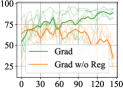
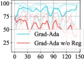
Figure 10: Ablation on the conservative regularization. The y-axis represents the normalize return, and the x-axis represents the number of gradient-ascent steps used for embedding inference at deployment. We plot each random seed as a transparent line; the solid line corresponds to the average across 5 seeds.

Note that our embedding inference depends on the learned score model $f$. Without proper regularization, such inference will lead to out-of-distribution embeddings that are erroneously high-scored ($\mathtt{Q2}$). Here we conduct an ablation study to examine the impact of the conservative regularization used for learning the score model.

In Figure 10, we compare DROP-Grad and DROP-Grad-Ada to their naive implementation (w/o Reg) that ablates the regularization on halfcheetah-medium-expert. We can find that removing the conservative regularization leads to unstable performance when changing the update steps of gradient-based optimization. However, we empirically find that in some tasks such a naive implementation (w/o Reg) does not necessarily bring unstable inference (Appendix C). Although improper gradient update step leads to faraway embeddings, to some extent, embedding-conditioned behavior policy can correct such deviation.

Appendix B Implementation Details

For the practical implementation of DROP, we parameterize the task embedding function $\phi(\mathbf{z}|n)$, the contextual behavior policy $\beta(\mathbf{a}|\mathbf{s},\mathbf{z})$, and the score model $f(\mathbf{s},\mathbf{a},\mathbf{z})$ with neural networks. For Equation 8 in the main paper, we construct a Lagrangian and solve the optimization through primal-dual gradient descent. For the choice of $\mu(\mathbf{z})$, we simply set $\mu(\mathbf{z})$ to be the uniform distribution over the $\mathcal{Z}$-space and empirically find that such uniform sampling can effectively avoid the out-of-distribution extrapolation at inference.

Lagrangian relaxation.

To optimize the constrained objective in Equation 8 in the main paper, we construct a Lagrangian and solve the optimization through primal-dual gradient descent,

$$\min_{f}\max_{\lambda>0}\quad \ \mathbb{E}_{\mathcal{D}_{n}\sim\mathcal{D}_{[N]}}\mathbb{E}_{(\mathbf{s},\mathbf{a},\mathbf{s}^{\prime},\mathbf{a}^{\prime})\sim\mathcal{D}_{n}}\left[\left(R(\mathbf{s},\mathbf{a})+\gamma\bar{f}(\mathbf{s}^{\prime},\mathbf{a}^{\prime},\phi(\mathbf{z}|n))-f(\mathbf{s},\mathbf{a},\phi(\mathbf{z}|n))\right)^{2}\right]+$$

$$\ \lambda\left(\mathbb{E}_{n,\mu(\mathbf{z})}\mathbb{E}_{\mathbf{s}\sim\mathcal{D}_{n},\mathbf{a}\sim\beta(\mathbf{a}|\mathbf{s},\mathbf{z})}\left[f(\mathbf{s},\mathbf{a},\mathbf{z})\right]-\mathbb{E}_{n,\phi(\mathbf{z}|n)}\mathbb{E}_{\mathbf{s}\sim\mathcal{D}_{n},\mathbf{a}\sim\beta(\mathbf{a}|\mathbf{s},\mathbf{z})}\left[f(\mathbf{s},\mathbf{a},\mathbf{z})\right]-\eta\right).$$

This unconstrained objective implies that if the expected difference in scores of out-of-distribution embeddings and in-distribution embeddings is less than a threshold $\eta$, $\lambda$ is going to be adjusted to $0$, on the contrary, $\lambda$ is likely to take a larger value, used to punish the over-estimated value function. This objective encourages that out-of-distribution embeddings score lower than in-distribution embeddings, thus performing embedding inference will not lead to these out-of-distribution embeddings that are falsely and over-optimistically scored by the learned score model.

In our experiments, we tried five different values for the Lagrange threshold $\eta$ ($1.0$, $2.0$, $3.0$, $4.0$, and $5.0$). We did not observe a significant difference in performance across these values. Therefore, we simply set $\eta=2.0$.

Hyper-parameters.

In Table 7, we provide the hyper-parameters of the task embedding $\phi(\mathbf{z}|\mathbf{s})$, the contextual behavior policy $\beta(\mathbf{a}|\mathbf{s},\mathbf{z})$, and the score function $f(\mathbf{s},\mathbf{a},\mathbf{z})$. For the gradient ascent update steps (used for embedding inference), we set $K=100$ for all the embedding inference rules in experiments.

Table 7: Hyper-parameters of the task embedding function $\phi(\mathbf{z}|\mathbf{s})$, the contextual behavior policy $\beta(\mathbf{a}|\mathbf{s},\mathbf{z})$, and the score function $f(\mathbf{s},\mathbf{a},\mathbf{z})$. The task embedding function $\phi(\mathbf{z}|\mathbf{s})$: $\mathbf{z}\leftarrow\text{Enc\_0}(n)$. The contextual behavior policy $\beta(\mathbf{a}|\mathbf{s},\mathbf{z})$: $\mathbf{a}\leftarrow\text{Enc\_2}(\mathbf{z},\text{Enc\_1}(\mathbf{s}))$. The score function $f(\mathbf{s},\mathbf{a},\mathbf{z})$: $f\leftarrow\text{Enc\_4}(\mathbf{z},\text{Enc\_3}(\mathbf{s},\mathbf{a}))$.

	Enc_0	Enc_1	Enc_2	Enc_3	Enc_4
Optimizer	Adam	Adam	Adam	Adam	Adam
Hidden layer	2	2	3	2	3
Hidden dim	512	512	512	512	512
Activation function	ReLU	ReLU	ReLU	ReLU	ReLU
Learning rate	1.00E-03	1.00E-03	1.00E-03	1.00E-03	1.00E-03
Mini-batch size	1024	1024	1024	1024	1024

In Table 9, we provide the number of sub-tasks, the number of trajectories in each sub-task, and the dimension of the embedding for each sub-task (behavior policy). The selection of hyperparameter N is based on two evaluation metrics: (1) the fitting loss of the decomposed behavioral policies to the offline data, and (2) the testing performance of DROP. Specifically,

• (Step1) Over a hyperparameter (the number of sub-tasks) set, we conduct the hyperparameter search using the fitting loss of behavior policies, then we choose/filter the four best hyperparameters;

• (Step2) We follow the normal practice of hyperparameter selection and tune the four hypermeters selected in Step1 by interacting with the simulator to estimate the performance of DROP under each hyperparameter setting.

Table 8: Hyperparameter (the number of sub-tasks) set.

tasks	the number of sub-tasks
Antmaze	500 (v0), 150 (v2)
Gym-mujoco	10, 20, 50, 100, 200, 500, 800, 1000
Adroit	10, 20, 50, 100, 200, 500, 800, 1000

We provide the hyperparameter sets in Table 8. In Step2, we tune the (filtered) hyperparameters using 1 seed, then evaluate the best hyperparameter by training on an additional 4 seeds and finally report the results on the 5 total seeds (see next "evaluation protocol"). In Antmaze domain, a single fixed N works well for many tasks; while in Gym-mujoco and Adroit domains, we did not find a fixed N that provides good results for all tasks in the corresponding domain in D4RL, thus we use the above hyperparameter selection rules (Step1 and Step2) to choose the number.

Baseline details.

For the comparison of our method to prior iterative offline RL methods, we consider the v0 versions of the datasets in D4RL. We take the baseline results of BEAR, BCQ, CQL, and BRAC-p from the D4RL paper [18], and take the results of TD3+BC from their origin paper [19]. For the comparison of our method to prior non-iterative offline RL method, we use the v2 versions of the dataset in D4RL. All the baseline results of behavior cloning (BC), Decision Transform (DT), RvS-R, and Onestep are taken from Emmons et al. [14]. In our implementation of COMs, we take the parameters (neural network weights) of behavior policies as the design input for the score model; and during testing, we conduct parameters inference (outer-level optimization) with 200 steps gradient ascent over the learned score function, then the rollout policy is initialized with the inferred parameters. For the specific architecture, we instantiate the policy network with $\mathrm{dim}(\mathcal{S})$ input units, two layers with 64 hidden units, and a final output layer with $\mathrm{dim}(\mathcal{A})$.

Evaluation protocol.

We evaluate our results over 5 seeds. For each seed, instead of taking the final checkpoint model produced by a training loop, we take the last $T$ ($T$ = 6 in our experiments) checkpoint models, and evaluate them over 10 episodes for each checkpoint. That is to say, we report the average of the evaluation scores over $5_{\text{seed}}\times 6_{\text{checkpoint}}\times 10_{\text{episode}}$ rollouts.

Algorithm 3 DROP: Online fine-tuning (checkpoint-level)

Require: Env, last $T$ checkpoint models: $\beta_{t}(\mathbf{a}|\mathbf{s},\mathbf{z})$ and $f_{t}(\mathbf{s},\mathbf{a},\mathbf{z})$ ($t=1,\cdots,T$).

1:  $R_{\text{MAX}}=-\infty$.

2:  $\beta_{\text{best}}\leftarrow\text{None}$.

3:  $f_{\text{best}}\leftarrow\text{None}$.

4:  while $t=1,\cdots,T$ do

5:     $\mathbf{s}_{0}$ = Env.Reset().

6:     ${\color[rgb]{0,0,0}\mathbf{z}^{*}_{0}(\mathbf{s}_{0})}$ $\leftarrow$ Conduct embedding inference with DROP-Best.

7:     Return $\leftarrow$ Evaluate $\beta_{t}$ and $f_{t}$ on Env, setting $\pi^{*}(\mathbf{a}|\mathbf{s})=\beta(\mathbf{a}|\mathbf{s},{\color[rgb]{0,0,0}\mathbf{z}^{*}_{0}(\mathbf{s}_{0})})$.

8:     if $R_{\text{MAX}}<\text{Return}$ then

9:        Update the best checkpoint models: $\beta_{\text{best}}\leftarrow\beta_{t}$, $f_{\text{best}}\leftarrow f_{t}$.

10:        Update the optimal return: $R_{\text{MAX}}\leftarrow\text{Return}$.

11:     end if

12:  end while

Return: $\beta_{\text{best}}$ and $f_{\text{best}}$.

Online fine-tuning (checkpoint-level): Instead of re-training the learned (final) policy with online rollouts, we fine-tune our policy with enumerated trial-and-error over the last $T$ checkpoint models (Algorithm 3). Specifically, for each seed, we run the last $T$ checkpoint models in the environment over one episode for each checkpoint. The checkpoint model which achieves the maximum episode return is returned. In essence, this fine-tuning procedure imitates the online RL evaluation protocol: if the current policy is unsatisfactory, we can use checkpoints of previous iterations of the policy.

Algorithm 4 DROP: Online fine-tuning (embedding-level)

Require: Env, last $T$ checkpoint models: $\beta_{t}(\mathbf{a}|\mathbf{s},\mathbf{z})$ and $f_{t}(\mathbf{s},\mathbf{a},\mathbf{z})$ ($t=1,\cdots,T$).

1:  $R_{\text{MAX}}=-\infty$.

2:  $\beta_{\text{best}}\leftarrow\text{None}$.

3:  $f_{\text{best}}\leftarrow\text{None}$.

4:  $k_{\text{best}}\leftarrow 0$.

5:  while $t=1,\cdots,T$ do

6:     while $k=1,\cdots,K_{\text{max}}$ do

7:        $\mathbf{s}_{0}$ = Env.Reset(). # Conduct embedding inference with DROP-Grad or DROP-Grad-Ada

8:        Return $\leftarrow$ Evaluate $\beta_{t}$ and $f_{t}$ on Env, setting $\pi^{*}(\mathbf{a}|\mathbf{s})=\beta(\mathbf{a}|\mathbf{s},{\color[rgb]{0,0,0}\mathbf{z}^{*}(\mathbf{s}_{0})})$ or $\beta(\mathbf{a}|\mathbf{s},{\color[rgb]{0,0,0}\mathbf{z}^{*}(\mathbf{s})})$, where we conduct $k$ gradient ascent steps to obtain ${\color[rgb]{0,0,0}\mathbf{z}^{*}(\mathbf{s}_{0})}$ or ${\color[rgb]{0,0,0}\mathbf{z}^{*}(\mathbf{s})}$.

9:        if $R_{\text{MAX}}<\text{Return}$ then

10:           Update the best checkpoint models: $\beta_{\text{best}}\leftarrow\beta_{t}$, $f_{\text{best}}\leftarrow f_{t}$.

11:           Update the best gradient update step: $k_{\text{best}}\leftarrow k$.

12:           Update the optimal return: $R_{\text{MAX}}\leftarrow\text{Return}$.

13:        end if

14:     end while

15:  end while

Return: $\beta_{\text{best}}$, $f_{\text{best}}$ and $k_{\text{best}}$.

Online fine-tuning (embedding-level): The embedding-level fine-tuning aims to find a suitable gradient ascent step that is used to conduct the embedding inference in DROP-Grad or DROP-Grad-Ada. Thus, we enumerate a list of gradient update steps and pick the best update step (according to the episode returns).

Codebase.

Our code is based on d3rlpy: https://github.com/takuseno/d3rlpy. We provide our source code in the supplementary material.

Computational resources.

The experiments were run on a computational cluster with 22x GeForce RTX 2080 Ti, and 4x NVIDIA Tesla V100 32GB for 20 days.

Table 9: The number ($N$) of sub-tasks, the number ($M$) of trajectories in each sub-task, and the dimension ($\mathrm{dim}(\mathbf{z})$) of the embedding for each sub-task.

Domain	Task Name	Parameters (*-v0)			Parameters (*-v2)
		$N$	$M$	$\mathrm{dim}(\mathbf{z})$	$N$	$M$	$\mathrm{dim}(\mathbf{z})$
Maze 2D	umaze	500	5	5
	medium	150	50	5
	large	100	15	5
Antmaze	umaze	500	50	5	150	50	5
	umaze-diverse	500	50	5	150	50	5
	Medium-play	500	50	5	150	50	5
	Medium-diverse	500	50	5	150	50	5
	Large-play	500	50	5	150	50	5
	Large-diverse	500	50	5	150	50	5
halfcheetah	random	1000	1	5	1000	1	5
	medium	100	2	5	100	2	5
	medium-expert	1000	1	5	1000	1	5
	medium-replay	50	10	5	50	10	5
hopper	random	100	2	5	100	2	5
	medium	100	5	5	100	5	5
	medium-expert	100	2	5	100	2	5
	medium-replay	50	5	5	10	30	5
walker2d	random	500	2	5	500	2	5
	medium	50	5	5	50	5	5
	medium-expert	50	5	5	50	5	5
	medium-replay	1000	5	5	10	50	5
door	cloned	1000	2	5
	expert	500	5	5
	human	50	3	5
hammer	cloned	1000	1	5
	expert	500	5	5
	human	20	3	5
pen	cloned	500	5	5
	expert	500	5	5
	human	50	5	5
relocate	cloned	500	5	5
	expert	500	5	5
	human	50	4	5

Appendix C Additional Results

Comparison with iterative offline RL baselines.

Here, we compare the performance of DROP (Grad, Best-Ada, and Grad-Ada ) to iterative offline RL baselines (BEAR [33], BCQ [20], CQL [35], BRAC-p [67], and TD3+BC [19]) that perform iterative bi-level offline RL paradigm with (explicit or implicit) value/policy regularization in inner-level. In Table 10, we present the results for AntMaze, Gym-MuJoCo, and Adroit suites in standard D4RL benchmark (*-v0), where we can find that DROP-Grad-Ada performs comparably or surpasses prior iterative bi-level works on most tasks: outperforming (or comparing) these policy regularized methods (BRAC-p and TD3+BC) on 25 out of 33 tasks and outperforming (or comparing) these value regularized algorithms (BEAR, BCQ, and CQL) on 19 out of 33 tasks.

Ablation studies.

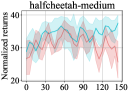
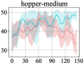
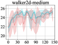
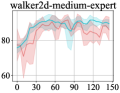
Figure 11: The performance comparison of DROP-Grad-Ada and DROP-Grad-Ada w/o Reg, where we ablate the conservative regularization for the w/o Reg implementation. The y-axis denotes the normalized return, the x-axis denotes the number of gradient-ascent steps used for embedding inference at deployment.

In Figure 11, we provide more results for the ablation of the conservative regularization term in Equation 8 in the main paper. We can find that for the halfcheetah-medium and hopper-medium tasks, the performance of DROP-Grad-Ada w/o Reg depends on the choice of the gradient update steps, showing that too small or too large number of gradient update step deteriorates the performance. Such a result is also consistent with COMs [62], which also observes the sensitivity of naive gradient update (i.e., w/o Reg) to the number of update steps used for design input inference. By comparison, the conservative score model learned with DROP-Grad-Ada exhibits more stable and robust performance to the gradient update steps.

Further, we also find that in walker2d-medium and walker2d-medium-expert tasks, the naive gradient update (w/o Reg) does not affect performance significantly across a wide range of gradient update steps. The main reason is that although the excessive gradient updates lead to faraway embeddings, conditioned on the inferred embeddings, the learned contextual behavior policy can safeguard against the embeddings distribution shift. Compared to prior model-based optimization that conducts direct gradient optimization (inference) over the design input itself, such "self-safeguard" is a special merit in the offline RL domain as long as we reframe the offline RL problem as one of model-based optimization and conduct inference over the embedding space. Thus, we encourage the research community to pursue further into this model-based optimization view for the offline RL problem.

Table 10: Comparison of our method to prior offline methods that perform iterative (regularized) RL paradigm on D4RL. We take the baseline results of BEAR, BCQ, CQL, and BRAC-p from Fu et al. [18], and the results of TD3-BC from Fujimoto and Gu [19]. For all results of our method (DROP), we average the normalized returns across 5 seeds; for each seed, we run 10 evaluation episodes. For proper comparison, we use $\blacktriangle$ and $\blacktriangle$ to denote DROP (*-Ada) achieves comparable or better performance compared with value and policy regularized offline RL methods respectively.

Task Name		Value Reg.			Policy Reg.		DROP-
		BEAR	BCQ	CQL	BRAC-p	TD3+BC	Grad	Best-Ada	Grad-Ada
antmaze	umaze	73.0	78.9	74.0	50.0	–	72.0$\blacktriangle$	78.0$\blacktriangle$$\blacktriangle$	80.0$\blacktriangle$$\blacktriangle$
	umaze-diverse	61.0	55.0	84.0	40.0	–	48.0$\blacktriangle$	62.0$\blacktriangle$$\blacktriangle$	66.0$\blacktriangle$$\blacktriangle$
	medium-play	0.0	0.0	61.2	0.0	–	24.0$\blacktriangle$	34.0$\blacktriangle$$\blacktriangle$	30.0$\blacktriangle$$\blacktriangle$
	medium-diverse	8.0	0.0	53.7	0.0	–	20.0$\blacktriangle$	24.0$\blacktriangle$$\blacktriangle$	30.0$\blacktriangle$$\blacktriangle$
	large-play	0.0	6.7	15.8	0.0	–	24.0$\blacktriangle$	36.0$\blacktriangle$$\blacktriangle$	42.0$\blacktriangle$$\blacktriangle$
	large-diverse	0.0	2.2	14.9	0.0	–	14.0$\blacktriangle$	20.0$\blacktriangle$$\blacktriangle$	26.0$\blacktriangle$$\blacktriangle$
halfcheetah	random	25.1	2.2	35.4	24.1	10.2	2.3$\blacktriangle$	2.3$\blacktriangle$$\blacktriangle$	2.3$\blacktriangle$$\blacktriangle$
	medium	41.7	40.7	44.4	43.8	42.8	42.4$\blacktriangle$	42.9$\blacktriangle$$\blacktriangle$	43.1$\blacktriangle$$\blacktriangle$
	medium-expert	53.4	64.7	62.4	44.2	97.9	86.6$\blacktriangle$	88.5$\blacktriangle$$\blacktriangle$	88.9$\blacktriangle$$\blacktriangle$
	medium-replay	38.6	38.2	46.2	45.4	43.3	39.5$\blacktriangle$	40.4$\blacktriangle$$\blacktriangle$	40.3$\blacktriangle$$\blacktriangle$
hopper	random	11.4	10.6	10.8	11.0	11.0	5.1$\blacktriangle$	5.4$\blacktriangle$$\blacktriangle$	5.5$\blacktriangle$$\blacktriangle$
	medium	52.1	54.5	58.0	32.7	99.5	57.5$\blacktriangle$	60.3$\blacktriangle$$\blacktriangle$	59.5$\blacktriangle$$\blacktriangle$
	medium-expert	96.3	110.9	98.7	1.9	112.2	103.5$\blacktriangle$	102.5$\blacktriangle$$\blacktriangle$	105.9$\blacktriangle$$\blacktriangle$
	medium-replay	33.7	33.1	48.6	0.6	31.4	48.0$\blacktriangle$	83.4$\blacktriangle$$\blacktriangle$	87.4$\blacktriangle$$\blacktriangle$
walker2d	random	7.3	4.9	7.0	-0.2	1.4	2.8$\blacktriangle$	3.0$\blacktriangle$$\blacktriangle$	3.0$\blacktriangle$$\blacktriangle$
	medium	59.1	53.1	79.2	77.5	79.7	76.5$\blacktriangle$	75.8$\blacktriangle$$\blacktriangle$	79.1$\blacktriangle$$\blacktriangle$
	medium-expert	40.1	57.5	111.0	76.9	101.1	107.5$\blacktriangle$	106.8$\blacktriangle$$\blacktriangle$	106.9$\blacktriangle$$\blacktriangle$
	medium-replay	19.2	15.0	26.7	-0.3	25.2	37.4$\blacktriangle$	60.9$\blacktriangle$$\blacktriangle$	61.9$\blacktriangle$$\blacktriangle$
door	cloned	-0.1	0.0	0.4	-0.1	–	0.5$\blacktriangle$	2.5$\blacktriangle$$\blacktriangle$	2.7$\blacktriangle$$\blacktriangle$
	expert	103.4	99.0	101.5	-0.3	–	98.6$\blacktriangle$	102.2$\blacktriangle$$\blacktriangle$	102.6$\blacktriangle$$\blacktriangle$
	human	-0.3	0.0	9.9	-0.3	–	3.3$\blacktriangle$	1.9$\blacktriangle$$\blacktriangle$	3.0$\blacktriangle$$\blacktriangle$
hammer	cloned	0.3	0.4	2.1	0.3	–	0.3$\blacktriangle$	0.3$\blacktriangle$$\blacktriangle$	0.3$\blacktriangle$$\blacktriangle$
	expert	127.3	107.2	86.7	0.3	–	65.7$\blacktriangle$	73.3$\blacktriangle$$\blacktriangle$	77.7$\blacktriangle$$\blacktriangle$
	human	0.3	0.5	4.4	0.3	–	1.1$\blacktriangle$	0.3$\blacktriangle$$\blacktriangle$	2.1$\blacktriangle$$\blacktriangle$
pen	cloned	26.5	44.0	39.2	1.6	–	76.7$\blacktriangle$	77.1$\blacktriangle$$\blacktriangle$	82.4$\blacktriangle$$\blacktriangle$
	expert	105.9	114.9	107.0	-3.5	–	113.1$\blacktriangle$	118.6$\blacktriangle$$\blacktriangle$	116.7$\blacktriangle$$\blacktriangle$
	human	-1.0	68.9	37.5	8.1	–	71.1$\blacktriangle$	85.2$\blacktriangle$$\blacktriangle$	81.5$\blacktriangle$$\blacktriangle$
relocate	cloned	-0.3	-0.3	-0.1	-0.3	–	0.1$\blacktriangle$	0.5$\blacktriangle$$\blacktriangle$	0.2$\blacktriangle$$\blacktriangle$
	expert	98.6	41.6	95.0	-0.3	–	2.5$\blacktriangle$	6.2$\blacktriangle$$\blacktriangle$	5.4$\blacktriangle$$\blacktriangle$
	human	-0.3	-0.1	0.2	-0.3	–	0.0$\blacktriangle$	0.0$\blacktriangle$$\blacktriangle$	0.0$\blacktriangle$$\blacktriangle$

References

- Abdolmaleki et al. [2018] Abbas Abdolmaleki, Jost Tobias Springenberg, Yuval Tassa, Remi Munos, Nicolas Heess, and Martin Riedmiller. Maximum a posteriori policy optimisation. arXiv preprint arXiv:1806.06920, 2018.
- Agarwal et al. [2021] Rishabh Agarwal, Max Schwarzer, Pablo Samuel Castro, Aaron C Courville, and Marc Bellemare. Deep reinforcement learning at the edge of the statistical precipice. Advances in neural information processing systems, 34:29304–29320, 2021.
- An et al. [2021] Gaon An, Seungyong Moon, Jang-Hyun Kim, and Hyun Oh Song. Uncertainty-based offline reinforcement learning with diversified q-ensemble. Advances in Neural Information Processing Systems, 34, 2021.
- Andrychowicz et al. [2017] Marcin Andrychowicz, Filip Wolski, Alex Ray, Jonas Schneider, Rachel Fong, Peter Welinder, Bob McGrew, Josh Tobin, OpenAI Pieter Abbeel, and Wojciech Zaremba. Hindsight experience replay. Advances in neural information processing systems, 30, 2017.
- Bai et al. [2022] Chenjia Bai, Lingxiao Wang, Zhuoran Yang, Zhihong Deng, Animesh Garg, Peng Liu, and Zhaoran Wang. Pessimistic bootstrapping for uncertainty-driven offline reinforcement learning. arXiv preprint arXiv:2202.11566, 2022.
- Brandfonbrener et al. [2021] David Brandfonbrener, Will Whitney, Rajesh Ranganath, and Joan Bruna. Offline rl without off-policy evaluation. Advances in Neural Information Processing Systems, 34:4933–4946, 2021.
- Brookes et al. [2019] David Brookes, Hahnbeom Park, and Jennifer Listgarten. Conditioning by adaptive sampling for robust design. In International conference on machine learning, pages 773–782. PMLR, 2019.
- Cang et al. [2021] Catherine Cang, Aravind Rajeswaran, Pieter Abbeel, and Michael Laskin. Behavioral priors and dynamics models: Improving performance and domain transfer in offline rl. arXiv preprint arXiv:2106.09119, 2021.
- Chebotar et al. [2021] Yevgen Chebotar, Karol Hausman, Yao Lu, Ted Xiao, Dmitry Kalashnikov, Jake Varley, Alex Irpan, Benjamin Eysenbach, Ryan Julian, Chelsea Finn, et al. Actionable models: Unsupervised offline reinforcement learning of robotic skills. arXiv preprint arXiv:2104.07749, 2021.
- Chen et al. [2021] Lili Chen, Kevin Lu, Aravind Rajeswaran, Kimin Lee, Aditya Grover, Misha Laskin, Pieter Abbeel, Aravind Srinivas, and Igor Mordatch. Decision transformer: Reinforcement learning via sequence modeling. Advances in neural information processing systems, 34, 2021.
- Chen et al. [2022] Xi Chen, Ali Ghadirzadeh, Tianhe Yu, Yuan Gao, Jianhao Wang, Wenzhe Li, Bin Liang, Chelsea Finn, and Chongjie Zhang. Latent-variable advantage-weighted policy optimization for offline rl. arXiv preprint arXiv:2203.08949, 2022.
- Chen et al. [2019] Xinyue Chen, Zijian Zhou, Zheng Wang, Che Wang, Yanqiu Wu, and Keith Ross. Bail: Best-action imitation learning for batch deep reinforcement learning. arXiv preprint arXiv:1910.12179, 2019.
- Ding et al. [2019] Yiming Ding, Carlos Florensa, Pieter Abbeel, and Mariano Phielipp. Goal-conditioned imitation learning. Advances in neural information processing systems, 32, 2019.
- Emmons et al. [2021] Scott Emmons, Benjamin Eysenbach, Ilya Kostrikov, and Sergey Levine. Rvs: What is essential for offline rl via supervised learning? arXiv preprint arXiv:2112.10751, 2021.
- Eysenbach et al. [2020] Ben Eysenbach, Xinyang Geng, Sergey Levine, and Russ R Salakhutdinov. Rewriting history with inverse rl: Hindsight inference for policy improvement. Advances in neural information processing systems, 33:14783–14795, 2020.
- Fannjiang and Listgarten [2020] Clara Fannjiang and Jennifer Listgarten. Autofocused oracles for model-based design. Advances in Neural Information Processing Systems, 33:12945–12956, 2020.
- Fu and Levine [2021] Justin Fu and Sergey Levine. Offline model-based optimization via normalized maximum likelihood estimation. arXiv preprint arXiv:2102.07970, 2021.
- Fu et al. [2020] Justin Fu, Aviral Kumar, Ofir Nachum, George Tucker, and Sergey Levine. D4RL: datasets for deep data-driven reinforcement learning. CoRR, abs/2004.07219, 2020. URL https://arxiv.org/abs/2004.07219.
- Fujimoto and Gu [2021] Scott Fujimoto and Shixiang Shane Gu. A minimalist approach to offline reinforcement learning. Advances in Neural Information Processing Systems, 34, 2021.
- Fujimoto et al. [2019] Scott Fujimoto, David Meger, and Doina Precup. Off-policy deep reinforcement learning without exploration. In International Conference on Machine Learning, pages 2052–2062. PMLR, 2019.
- Furuta et al. [2021] Hiroki Furuta, Yutaka Matsuo, and Shixiang Shane Gu. Generalized decision transformer for offline hindsight information matching. arXiv preprint arXiv:2111.10364, 2021.
- Geist et al. [2019] Matthieu Geist, Bruno Scherrer, and Olivier Pietquin. A theory of regularized markov decision processes. In Kamalika Chaudhuri and Ruslan Salakhutdinov, editors, Proceedings of the 36th International Conference on Machine Learning, ICML 2019, 9-15 June 2019, Long Beach, California, USA, volume 97 of Proceedings of Machine Learning Research, pages 2160–2169. PMLR, 2019.
- Ghosh et al. [2022] Dibya Ghosh, Anurag Ajay, Pulkit Agrawal, and Sergey Levine. Offline rl policies should be trained to be adaptive. In International Conference on Machine Learning, pages 7513–7530. PMLR, 2022.
- Gulcehre et al. [2021] Caglar Gulcehre, Sergio Gómez Colmenarejo, Ziyu Wang, Jakub Sygnowski, Thomas Paine, Konrad Zolna, Yutian Chen, Matthew Hoffman, Razvan Pascanu, and Nando de Freitas. Regularized behavior value estimation. arXiv preprint arXiv:2103.09575, 2021.
- Janner et al. [2021] Michael Janner, Qiyang Li, and Sergey Levine. Offline reinforcement learning as one big sequence modeling problem. Advances in neural information processing systems, 34, 2021.
- Janner et al. [2022] Michael Janner, Yilun Du, Joshua B Tenenbaum, and Sergey Levine. Planning with diffusion for flexible behavior synthesis. arXiv preprint arXiv:2205.09991, 2022.
- Jin et al. [2021] Ying Jin, Zhuoran Yang, and Zhaoran Wang. Is pessimism provably efficient for offline rl? In International Conference on Machine Learning, pages 5084–5096. PMLR, 2021.
- Kang et al. [2023] Yachen Kang, Diyuan Shi, Jinxin Liu, Li He, and Donglin Wang. Beyond reward: Offline preference-guided policy optimization. arXiv preprint arXiv:2305.16217, 2023.
- Kidambi et al. [2020] Rahul Kidambi, Aravind Rajeswaran, Praneeth Netrapalli, and Thorsten Joachims. Morel: Model-based offline reinforcement learning. Advances in neural information processing systems, 33:21810–21823, 2020.
- Kostrikov et al. [2021a] Ilya Kostrikov, Rob Fergus, Jonathan Tompson, and Ofir Nachum. Offline reinforcement learning with fisher divergence critic regularization. In International Conference on Machine Learning, pages 5774–5783. PMLR, 2021a.
- Kostrikov et al. [2021b] Ilya Kostrikov, Ashvin Nair, and Sergey Levine. Offline reinforcement learning with implicit q-learning. arXiv preprint arXiv:2110.06169, 2021b.
- Kumar and Levine [2020] Aviral Kumar and Sergey Levine. Model inversion networks for model-based optimization. Advances in Neural Information Processing Systems, 33:5126–5137, 2020.
- Kumar et al. [2019a] Aviral Kumar, Justin Fu, Matthew Soh, George Tucker, and Sergey Levine. Stabilizing off-policy q-learning via bootstrapping error reduction. Advances in Neural Information Processing Systems, 32, 2019a.
- Kumar et al. [2019b] Aviral Kumar, Xue Bin Peng, and Sergey Levine. Reward-conditioned policies. arXiv preprint arXiv:1912.13465, 2019b.
- Kumar et al. [2020] Aviral Kumar, Aurick Zhou, George Tucker, and Sergey Levine. Conservative q-learning for offline reinforcement learning. Advances in Neural Information Processing Systems, 33:1179–1191, 2020.
- Lai et al. [2023] Yao Lai, Jinxin Liu, Zhentao Tang, Bin Wang, HAO Jianye, and Ping Luo. Chipformer: Transferable chip placement via offline decision transformer. ICML, 2023. URL https://openreview.net/pdf?id=j0miEWtw87.
- Lange et al. [2012] Sascha Lange, Thomas Gabel, and Martin Riedmiller. Batch reinforcement learning. In Reinforcement learning, pages 45–73. Springer, 2012.
- LeCun et al. [2006] Yann LeCun, Sumit Chopra, Raia Hadsell, M Ranzato, and F Huang. A tutorial on energy-based learning. Predicting structured data, 1(0), 2006.
- Lee et al. [2021] Jongmin Lee, Wonseok Jeon, Byungjun Lee, Joelle Pineau, and Kee-Eung Kim. Optidice: Offline policy optimization via stationary distribution correction estimation. In International Conference on Machine Learning, pages 6120–6130. PMLR, 2021.
- Levine et al. [2020] Sergey Levine, Aviral Kumar, George Tucker, and Justin Fu. Offline reinforcement learning: Tutorial, review, and perspectives on open problems. arXiv preprint arXiv:2005.01643, 2020.
- Li et al. [2022] Jinning Li, Chen Tang, Masayoshi Tomizuka, and Wei Zhan. Dealing with the unknown: Pessimistic offline reinforcement learning. In Conference on Robot Learning, pages 1455–1464. PMLR, 2022.
- Lin et al. [2022] Qinjie Lin, Han Liu, and Biswa Sengupta. Switch trajectory transformer with distributional value approximation for multi-task reinforcement learning. arXiv preprint arXiv:2203.07413, 2022.
- Liu et al. [2021] Jinxin Liu, Hao Shen, Donglin Wang, Yachen Kang, and Qiangxing Tian. Unsupervised domain adaptation with dynamics-aware rewards in reinforcement learning. Advances in Neural Information Processing Systems, 34:28784–28797, 2021.
- Liu et al. [2022a] Jinxin Liu, Donglin Wang, Qiangxing Tian, and Zhengyu Chen. Learn goal-conditioned policy with intrinsic motivation for deep reinforcement learning. In Proceedings of the AAAI Conference on Artificial Intelligence (AAAI), volume 36, pages 7558–7566, 2022a.
- Liu et al. [2022b] Jinxin Liu, Hongyin Zhang, and Donglin Wang. Dara: Dynamics-aware reward augmentation in offline reinforcement learning. arXiv preprint arXiv:2203.06662, 2022b.
- Liu et al. [2023] Jinxin Liu, Ziqi Zhang, Zhenyu Wei, Zifeng Zhuang, Yachen Kang, Sibo Gai, and Donglin Wang. Beyond ood state actions: Supported cross-domain offline reinforcement learning. arXiv preprint arXiv:2306.12755, 2023.
- Liu et al. [2019] Yao Liu, Adith Swaminathan, Alekh Agarwal, and Emma Brunskill. Off-policy policy gradient with state distribution correction. arXiv preprint arXiv:1904.08473, 2019.
- Ma et al. [2021a] Xiaoteng Ma, Yiqin Yang, Hao Hu, Qihan Liu, Jun Yang, Chongjie Zhang, Qianchuan Zhao, and Bin Liang. Offline reinforcement learning with value-based episodic memory. arXiv preprint arXiv:2110.09796, 2021a.
- Ma et al. [2021b] Yecheng Ma, Dinesh Jayaraman, and Osbert Bastani. Conservative offline distributional reinforcement learning. Advances in Neural Information Processing Systems, 34, 2021b.
- Matsushima et al. [2020] Tatsuya Matsushima, Hiroki Furuta, Yutaka Matsuo, Ofir Nachum, and Shixiang Gu. Deployment-efficient reinforcement learning via model-based offline optimization. arXiv preprint arXiv:2006.03647, 2020.
- Nachum et al. [2019] Ofir Nachum, Bo Dai, Ilya Kostrikov, Yinlam Chow, Lihong Li, and Dale Schuurmans. Algaedice: Policy gradient from arbitrary experience. arXiv preprint arXiv:1912.02074, 2019.
- Nair et al. [2020a] Ashvin Nair, Murtaza Dalal, Abhishek Gupta, and Sergey Levine. Accelerating online reinforcement learning with offline datasets. arXiv preprint arXiv:2006.09359, 2020a.
- Nair et al. [2020b] Ashvin Nair, Abhishek Gupta, Murtaza Dalal, and Sergey Levine. Awac: Accelerating online reinforcement learning with offline datasets. arXiv preprint arXiv:2006.09359, 2020b.
- Peng et al. [2019] Xue Bin Peng, Aviral Kumar, Grace Zhang, and Sergey Levine. Advantage-weighted regression: Simple and scalable off-policy reinforcement learning. arXiv preprint arXiv:1910.00177, 2019.
- Pong et al. [2018] Vitchyr Pong, Shixiang Gu, Murtaza Dalal, and Sergey Levine. Temporal difference models: Model-free deep rl for model-based control. arXiv preprint arXiv:1802.09081, 2018.
- Rezaeifar et al. [2021] Shideh Rezaeifar, Robert Dadashi, Nino Vieillard, Léonard Hussenot, Olivier Bachem, Olivier Pietquin, and Matthieu Geist. Offline reinforcement learning as anti-exploration. arXiv preprint arXiv:2106.06431, 2021.
- Rigter et al. [2022] Marc Rigter, Bruno Lacerda, and Nick Hawes. Rambo-rl: Robust adversarial model-based offline reinforcement learning. arXiv preprint arXiv:2204.12581, 2022.
- Siegel et al. [2020] Noah Y Siegel, Jost Tobias Springenberg, Felix Berkenkamp, Abbas Abdolmaleki, Michael Neunert, Thomas Lampe, Roland Hafner, Nicolas Heess, and Martin Riedmiller. Keep doing what worked: Behavioral modelling priors for offline reinforcement learning. arXiv preprint arXiv:2002.08396, 2020.
- Silver et al. [2014] David Silver, Guy Lever, Nicolas Heess, Thomas Degris, Daan Wierstra, and Martin Riedmiller. Deterministic policy gradient algorithms. In International conference on machine learning, pages 387–395. PMLR, 2014.
- Srivastava et al. [2019] Rupesh Kumar Srivastava, Pranav Shyam, Filipe Mutz, Wojciech Jaśkowski, and Jürgen Schmidhuber. Training agents using upside-down reinforcement learning. arXiv preprint arXiv:1912.02877, 2019.
- Sutton and Barto [2018] Richard S Sutton and Andrew G Barto. Reinforcement learning: An introduction. MIT press, 2018.
- Trabucco et al. [2021] Brandon Trabucco, Aviral Kumar, Xinyang Geng, and Sergey Levine. Conservative objective models for effective offline model-based optimization. In International Conference on Machine Learning, pages 10358–10368. PMLR, 2021.
- Trabucco et al. [2022] Brandon Trabucco, Xinyang Geng, Aviral Kumar, and Sergey Levine. Design-bench: Benchmarks for data-driven offline model-based optimization. arXiv preprint arXiv:2202.08450, 2022.
- Vieillard et al. [2020] Nino Vieillard, Tadashi Kozuno, Bruno Scherrer, Olivier Pietquin, Rémi Munos, and Matthieu Geist. Leverage the average: an analysis of KL regularization in reinforcement learning. In Hugo Larochelle, Marc’Aurelio Ranzato, Raia Hadsell, Maria-Florina Balcan, and Hsuan-Tien Lin, editors, Advances in Neural Information Processing Systems 33: Annual Conference on Neural Information Processing Systems 2020, NeurIPS 2020, December 6-12, 2020, virtual, 2020.
- Wan et al. [2021] Michael Wan, Jian Peng, and Tanmay Gangwani. Hindsight foresight relabeling for meta-reinforcement learning. arXiv preprint arXiv:2109.09031, 2021.
- Wang et al. [2020] Ziyu Wang, Alexander Novikov, Konrad Zolna, Jost Tobias Springenberg, Scott Reed, Bobak Shahriari, Noah Siegel, Josh Merel, Caglar Gulcehre, Nicolas Heess, et al. Critic regularized regression. arXiv preprint arXiv:2006.15134, 2020.
- Wu et al. [2019] Yifan Wu, George Tucker, and Ofir Nachum. Behavior regularized offline reinforcement learning. arXiv preprint arXiv:1911.11361, 2019.
- Wu et al. [2021] Yue Wu, Shuangfei Zhai, Nitish Srivastava, Joshua Susskind, Jian Zhang, Ruslan Salakhutdinov, and Hanlin Goh. Uncertainty weighted actor-critic for offline reinforcement learning. arXiv preprint arXiv:2105.08140, 2021.
- Yang et al. [2022] Rui Yang, Yiming Lu, Wenzhe Li, Hao Sun, Meng Fang, Yali Du, Xiu Li, Lei Han, and Chongjie Zhang. Rethinking goal-conditioned supervised learning and its connection to offline rl. arXiv preprint arXiv:2202.04478, 2022.
- Yu et al. [2021a] Sihyun Yu, Sungsoo Ahn, Le Song, and Jinwoo Shin. Roma: Robust model adaptation for offline model-based optimization. Advances in Neural Information Processing Systems, 34, 2021a.
- Yu et al. [2020] Tianhe Yu, Garrett Thomas, Lantao Yu, Stefano Ermon, James Y Zou, Sergey Levine, Chelsea Finn, and Tengyu Ma. Mopo: Model-based offline policy optimization. Advances in Neural Information Processing Systems, 33:14129–14142, 2020.
- Yu et al. [2021b] Tianhe Yu, Aviral Kumar, Rafael Rafailov, Aravind Rajeswaran, Sergey Levine, and Chelsea Finn. Combo: Conservative offline model-based policy optimization. Advances in neural information processing systems, 34:28954–28967, 2021b.
- Zhang et al. [2021] Chi Zhang, Sanmukh Kuppannagari, and Prasanna Viktor. Brac+: Improved behavior regularized actor critic for offline reinforcement learning. In Asian Conference on Machine Learning, pages 204–219. PMLR, 2021.
- Zhou et al. [2020] Wenxuan Zhou, Sujay Bajracharya, and David Held. Plas: Latent action space for offline reinforcement learning. arXiv preprint arXiv:2011.07213, 2020.
- Zhuang et al. [2023] Zifeng Zhuang, Kun Lei, Jinxin Liu, Donglin Wang, and Yilang Guo. Behavior proximal policy optimization. arXiv preprint arXiv:2302.11312, 2023.