Quantum fluctuations lead to glassy electron dynamics in a good metal

Abstract

One of the central challenges in condensed matter physics is to comprehend systems that have strong disorder and strong interactions. In the strongly localized regime, their subtle competition engenders glassy electrons, which ceases to exist well before the insulator-to-metal transition is approached as a function of doping. Here, we report on the discovery of glassy electron dynamics deep inside the good metal regime of an electron-doped quantum paraelectric system: KTaO₃. We reveal that upon excitation of electrons from defect states to the conduction band, the excess injected carriers in the conduction band relax in a stretched exponential manner with a large relaxation time, and the system evinces simple aging phenomena - a telltale sign of glass. Most significantly, we observe a critical slowing down of carrier dynamics below 35 K, concomitant with the onset of quantum paraelectricity in the undoped KTaO₃. Our combined investigation using second harmonic generation technique, density functional theory and phenomenalogical modeling demonstrates quantum fluctuation-stabilized soft polar modes as the impetus for the glassy behavior. This study addresses one of the most fundamental questions regarding the potential promotion of glassiness by quantum fluctuations and opens a route for exploring glassy dynamics of electrons in a well-delocalized regime.

Introduction: The notion of glassy dynamics associated with the electronic degree of freedom in condensed matter systems was first envisaged by Davies, Lee and Rice in 1982 [1]. Building heavily on Anderson’s seminal work on the localization of wave functions in random disordered media [2], it was predicted that, in a disordered insulator with highly localized electronic states, the interplay between disorder and long-range Coulomb interaction (Fig. 1a) should precipitate electronic frustration in real space. Such a scenario would result in a rugged energy landscape with numerous metastable states, leading to the emergence of electron glass [3, 4, 5]. This hypothesis was soon tested on various strongly localized electronic systems, including granular metals, crystalline and amorphous oxides, and later, it was also extended to doped semiconductors and two-dimensional electron gases [6, 3, 4, 5, 7]. The typical relaxation time in these systems ranges from a few seconds to several hours, making them an obvious choice for studying glassy physics in laboratory timescales. What makes these systems even more intriguing is the array of perturbations that one can use to effectively drive them away from equilibrium [4]. Moreover, electron glasses are highly susceptible to quantum effects, making them an ideal platform for investigating the potential role of quantum fluctuations in the formation or melting of glasses, which has remained a pervasive problem in the field of glass [8, 9].

In the antithetical regime of highly delocalized electrons i.e. in a metal, the screening effect significantly reduces the strength of the electron-electron and electron-impurity interactions. Consequently, such system generally possesses a non-degenerate ground state with a well-defined Fermi surface. As a result, the dynamics of glassy behavior, which involves the existence of multiple, competing ground states, is incompatible with the behavior of metals. In fact, the manifestation of glassiness fades away considerably prior to the transition from insulator to metal, and there is an absolute lack of any substantiated indication of the presence of glassiness within a good metal regime [3] where quasi-particle mean free path is larger than the electron’s wavelength.

In this work, we report on the discovery of glassy dynamics of conduction electrons in an electron-doped quantum paraelectric system, namely KTaO₃, in a good metal regime. Even more surprising observation is that glassiness is found to appear in a regime where quantum fluctuations are inherently present in the system. In pristine KTaO₃, the quantum fluctuations associated with the zero point motion of the atoms prohibits the onset of ferroelectric order below 35 K (Fig. 1b), and the system’s properties are typically governed by the presence of associated low energy transverse optical phonon (Fig. 1c) popularly known as soft polar mode [13]. Our combined transport and optical second harmonic generation measurements find that properties associated with the soft polar mode are preserved even deep inside the metallic regime. Most importantly, such soft modes are found to be directly responsible for emergent glassy dynamics at low temperatures, which is further corroborated by our theoretical calculations. Our observation is one of the rarest examples where quantum fluctuation, which is generally considered as a bottleneck for glass formation [8, 9], is ultimately accountable for the appearance of glassy dynamics in a good metallic phase.

Demonstration of good metallic behavior: Several successful attempts have been made in recent times to introduce free carriers in the bulk as well as at the surface or interface of KTaO₃ [14, 15, 16, 17]. For the current investigation, metallic samples have been prepared by introducing oxygen vacancies in pristine single crystalline (001) oriented KTaO₃ substrate (for details see methods section and references  [11, 18]). These samples were found to exhibit quantum oscillations below 10 K, which is signature of a good metal with well defined Fermi surface. To further testify this, we have also computed temperature-dependent mean free path of electrons ($l_{e}$) within Drude–Boltzmann picture. Fig. 1c shows the corresponding plots for degenerate and non-degenerate case. A dotted vertical line marks the temperature above which $l_{e}$ becomes shorter than the inverse of Fermi wave-vector ($k_{F}$) and the sample crosses over from normal metal to a bad metal phase [12]. In the current work, observation of glassy dynamics is inherently constrained to temperatures which is much lower than crossover temperature to bad metal phase and hence for all practical purposes our electron doped KTaO₃ system can be considered as a good metal with well-defined scattering.

Demonstration of glassy dynamics: Oxygen vacancy creation in KTaO₃ not only adds free electrons but also leads to the formation of highly localized defect states. To determine the exact position of the defect states, valence band spectrum has been mapped out by using hard X-ray photoelectron spectroscopy (HAXPES) at P22 beamline of PETRA III, DESY (see methods for more details). Apart from the well-defined quasi-particle peak, mid-gap states centered at 1.6-1.8 eV is observed (Fig. 2a), which arises due to the clustering of oxygen vacancies [18].

In this work, we utilize these defect states to perturb the system by selective excitation of trapped electrons to the conduction band via sub-bandgap light illumination. Subsequently, the system’s response is studied by monitoring the temporal evolution of the electrical resistance at a fixed temperature (see inset of Fig. 2a for transport measurement set-up). For each measurement, the sample was first cooled down to the desired temperature. Once the temperature stabilizes, the system was driven out of equilibrium by shining light for half an hour, thereafter resistance relaxation was observed for the next 1.5 hours in dark condition. For the next measurement, the sample was heated to room temperature where the original resistance is recovered. Fig. 2b shows one set of data recorded with green light ($\lambda$=527 nm) at several fixed temperatures ranging from 15 K to 150 K.

At first glance, Fig. 2b reveals a striking temperature dependence of the photo-doping effect (also see Supplementary Information Section 1 and Supplementary Fig. 1) and the way the system relaxes after turning off the light is also found to be strongly temperature dependent. Further analysis reveals that in the off-stage, the resistance relaxes in a stretched exponential manner [exp(-($t$/$\tau$)^β) where $\tau$ is the relaxation time and $\beta$ (stretching exponent) $<$ 1 (Fig. 2c)], signifying the presence of multiple relaxation channels for the electron-hole recombination [20]. The microscopic origin behind the spatial separation of electron-hole pair and resultant non-exponential relaxation will be discussed later. The temperature evolution of $\beta$ and $\tau$ obtained from the fitting further reveals a substantial increase in relaxation time followed by constant $\beta\approx$ 0.5 below 35 K (Fig. 2c). This observation is remarkable given the fact that this crossover temperature precisely coincides with the onset of quantum fluctuation in undoped KTaO₃. Such stretched exponential relaxation with $\beta$ less than 1 is very often considered as a signature of glassy dynamics and has been observed in variety of systems [4, 21, 22].

One critical test to confirm a glassy phase is the observation of aging phenomenon wherein the system’s response depends on its age [23]. More precisely, older systems are found to relax more slowly than younger ones. To examine this, we prepared the system of desired age by tuning the duration of light illumination ($t$${}_{\text{ill}}$), and measurements similar to that shown in Fig. 2b were performed at 15 K (Fig. 3a ). For further analysis, we only focus on relaxation after turning off the light. In Fig. 3b we plot the change in resistance in the off-stage ($\Delta$$R$${}_{\text{off}}$) normalized with a total drop in resistance ($\Delta$$R$${}_{\text{ill}}$) at the end of illumination. Evidently, with increasing $t$${}_{\text{ill}}$ system’s response becomes more and more sluggish. More precisely, $\tau$ obtained from the fitting is found to scale linearly with $t$${}_{\text{ill}}$ (inset of Fig. 3c). This is the defining criteria for simple or full aging [23] which is more clear in Fig. 3c where all the curves can be collapsed to a universal curve by normalizing the abscissa by $t$${}_{\text{ill}}$. A careful look at Fig. 3c reveals that for larger values of $t$${}_{\text{ill}}$, curves start to deviate from the universal scaling. This is much clear in Fig. 3d which contains a similar set of scaling data for another sample with a different carrier concentration. Such an observation is consistent with the criteria for aging that $t$${}_{\text{ill}}$ should be much less than the time required to reach the new equilibrium under perturbation. As evident from Fig. 3a and inset of Fig. 3d, above a critical value of $t$${}_{\text{ill}}$ there is little change in resistance upon shining the light any further. This signifies that the system is closer to its new equilibrium and hence aging ceases to hold at a higher $t$${}_{\text{ill}}$.

Presence of polar nano regions & importance of quantum fluctuations: As mentioned earlier, the glassy behavior of electrons in conventional electron glasses results from the competition between disorder and Coulomb interactions and is only applicable in strongly localized regime [3, 4, 5]. As glassiness is observed within a good metal regime ($k_{F}$$l_{e}$$>$1) in our oxygen-deficient KTaO₃ samples, we need to find other processes responsible for the electron-hole separation and complex glassy relaxations in the present case. In the context of electron doping in another well-studied quantum paraelectric SrTiO₃, a large lattice relaxation (LLR) model involving deep trap levels [24] has been associated as a dominant cause for prohibiting electron-hole recombination [25, 26]. However, our analysis of $\tau$ vs. $T$ (Supplementary Information Section 4 and Supplementary Fig. 4) does not support the applicability of the LLR model in the present case. In sharp contrast, we will conclusively demonstrate here that the effective charge separation in such systems directly correlates with the appearance of polar nano regions (PNRs), which arise as a direct consequence of the defect dipoles present in a highly polarizable lattice of quantum paraelectric [27].

In an ordinary dielectric host, an electric dipole can polarize the lattice only in its immediate vicinity and the correlation length ($r_{c}$) is generally of the order of unit cell length which further remains independent of temperature [6]. However the situation is drastically different in highly polarizable hosts such as KTaO₃ where the magnitude of $r_{c}$ is controlled by the polarizability of the lattice which is inversely proportional to the soft mode frequency ($\omega$_s). Since $\omega$_s decreases with decreasing temperature, $r_{c}$ becomes large at lower temperatures. As a result, PNRs spanning several unit cells are formed around the defect dipole which is randomly distributed in the lattice (Fig. 4a).

While PNRs are quite well established in the insulating regime (Supplementary Information Section 5 and Supplementary Fig. 5), they are expected to vanish in the metals due to screening effects from free electrons. Surprisingly, several recent experiments have reported that PNRs can exist even in the metallic regime [29, 30, 31, 32, 33]. Motivated by these results, we have carried out temperature-dependent optical second harmonic generation (SHG) measurement (Fig. 4b) which is a powerful technique to probe PNRs [9]. Fig. 4c shows the temperature evolution of SHG intensity which is directly proportional to the volume density of PNRs. As evident, no appreciable SHG signal is observed at room temperature, however a strong signal enhancement is observed below 150 K, signifying the appearance of PNR below 150 K in our metallic sample. Since this onset temperature exactly coincides with the temperature below which an appreciable photo-doping effect is observed in our photo conductivity measurements (Supplementary Information Section 6 and Supplementary Fig. 6), we believe that the internal electric field generated around such PNRs is the major cause behind driving apart the photo-generated electron-hole pairs in real space. Another notable observation is that the SHG intensity is independent of the temperature below 35 K. Since $r_{c}\propto\omega_{s}^{-1}$ [13], our SHG measurement establishes that quantum fluctuation stabilized soft polar mode is retained even in metallic KTaO₃ [35].

We have also conducted an investigation into the primary defect dipoles responsible for the creation of PNRs in our samples. Considering that our samples were prepared through high-temperature annealing within an evacuated sealed quartz tube [18], there is a possibility of K vacancies due to its high volatility. The presence of a certain degree of K vacancy has been indeed observed in our HAXPES measurements (Supplementary Information Section 7 and Supplementary Fig. 7). It is widely established that, in $AB$O₃ systems, the off-centering of substitute $B$ atom ($B$ antisite-like defect) in the presence of $A$ atom vacancy leads to a macroscopic polarization even in a non-polar matrix  [36, 37, 9, 38, 39]. Our density functional theory calculations (details are in the method section) considering Ta antisite-like defect has found significant Ta off-centering along [100] and [110] in the presence of K vacancy (Fig. 4d). Further, we have also computed induced polarization in the system following the modern theory of polarization where the change in macroscopic electric polarization is represented by a Berry phase [12, 15, 42, 13, 44] and the non-zero Berry curvature i.e., Berry phase per unit area, is taken as a signature of finite polarization in the material. In Fig.4e, f, we have plotted the Berry curvature in the plane $k_{z}=0$ ($\Omega_{xy}(\mathbf{k})$) for the Ta off-centering along [110] and [100], respectively. From the figure, it is clear that the large contributions to the Berry curvature are due to the avoided crossings of bands at the Fermi surface (see inset of Fig. 4f) which are induced by spin-orbit coupling.

Phenomenological model to understand glassy dynamics: We now discuss a possible mechanism for the emergent glassy dynamics in a metal where conduction electrons coexist with PNRs. Since the glassiness in the present case is observed in the dynamical relaxation of excess injected carriers in the conduction band, it is necessary to have a thorough understanding of the relaxation processes happening against the backdrop of randomly oriented PNRs. In indirect-band semiconductors like KTaO₃ which have strong electron-lattice and defect-lattice coupling, the relaxation should be predominantly nonradiative and manifest itself as the emission of several low-energy phonons [45]. Further, since inter-band electron-phonon matrix element due to acoustic phonons are negligible, the electron-hole recombination may primarily involve soft polar modes at low temperatures, although it is not the lowest energy phonon [46]. While such a multi-phonon inter-band transition could lead to multichannel relaxation with large time scales [45], it can never give rise to collective glassy behavior.

Instead, we suggest the following scenario for the observed glassiness. As was previously mentioned, there is clear evidence that the internal electric field around PNRs has a significant impact on electron-hole recombination in our sample. It has been demonstrated previously [27] that the random interactions between PNRs (in the limit of dilute defect dipoles) leads to a dipole glass at low temperatures in KTaO₃. Electrons and holes being charged particles would immediately couple to the complex electric field from the dipole glass and hence there is a chance that the glassy background of PNRs can induce glassiness to the free carriers in the system.

In order to study such a possibility, we consider a theoretical model with the Hamiltonian,

$$H =H_{el}+H_{gl}+H_{el-gl},$$ (1)

where $H_{el}=-\sum_{ij}t_{ij}c_{i}^{\dagger}c_{j}-\varepsilon_{0}\sum_{\alpha}f_{\alpha}^{\dagger}f_{\alpha}$ ($\varepsilon_{0}>0$) describes the electronic part in terms of creation and annihilation operators $c_{i}^{\dagger},c_{i}$ ($i=1,\cdots,N_{c}$) and $f_{\alpha}^{\dagger},f_{\alpha}$ ($\alpha=1,\cdots,N_{f}$) of the $N_{c}$ conduction and $N_{f}$ impurity electronic states, respectively. For our calculations, we consider various lattices and corresponding hopping amplitudes $t_{ij}$ to describe several different energy dispersions for the conduction band, e.g., a band with semicircular DOS $g(\epsilon)=(1/2\pi)\sqrt{W^{2}-\omega^{2}}\theta(W-|\omega|)$ with band width $W$ [$\theta(x)$ is heaviside step function] (Fig. 5(a)), and a flat band with width $W=0$, as discussed in the Supplementary Information Section 9. We take a flat impurity band at energy $-\varepsilon_{0}$, separated by a gap $\Delta=\varepsilon_{0}-W/2$ from the conduction band minimum. We set the chemical potential $\mu=0$, at the centre of conduction band (Fig. 5(a)).

To model the dynamics of the glassy background, which may result from either a single PNR or randomly-distributed coupled assembly of PNRs, we consider a system with $N_{g}$ degrees of freedom $\{x_{\mu}\}$ (Supplementary Information Section 9). These position-like variables, related to the electric dipoles inside the PNRs, can be thought of as a multi-coordinate generalization of the usual single configuration coordinate  [24, 45, 26] for a defect or impurity in semiconductors. Such single coordinate defect model, though can give rise to very slow relaxation of photoresistivity [24, 45, 26], is unlikely to lead to collective aging phenomena seen in our experiment. For our model, we thus assume a collective glassy background that gives rise to a two-step relaxation, $C_{gl}(t)=\langle x_{\mu}(t)x_{\mu}(0)\rangle=A\exp(-t/\tau_{s})+B\exp[-(t/\tau_{\alpha})^{\beta}]$ as a function of time $t$, for the dynamical correlation of $x_{\mu}$ at temperature $T$. The relaxation consists of a short-time exponential decay with the time scale $\tau_{s}$ and a long-time stretched exponential $\alpha$-relaxation with time scale $\tau_{\alpha}(T)$ and stretching exponent $\beta$ [47, 48]. We assume that $\tau_{s}$ is temperature independent, whereas $\tau_{\alpha}$ increases with decreasing temperature. We also vary the coefficients $A(T)$ and $B(T)$ with $T$ such that the relative strength of the stretched exponential part increases at lower temperatures (Supplementary Information Section 9).

The glassy PNRs lead to a transition between the conduction band and impurity state via a coupling $H_{el-gl}=\sum_{i\alpha\mu}(V_{i\alpha\mu}c_{i}^{\dagger}f_{\alpha}+\mathrm{h.c})x_{\mu}$, where we take $V_{i\alpha\mu}$ as Gaussian complex random numbers to keep the model solvable. The coupling can arise either due to direct coupling of the electric field of the PNR to the electrons, or indirectly via coupling between PNR and electrons mediated by phonons, e.g., the soft polar optical phonon mode.

To gain an analytical understanding of the electron-hole recombination dynamics we consider a limit where there are no backactions of the conduction electrons on the impurity electrons and the glass (Supplementary Information Section 9).

The description of the relaxation of the photo-excited electrons requires the consideration of the out-of-equilibrium quantum dynamics, which is beyond the scope of this paper. Instead, we consider an equilibrium dynamical correlation, namely the (connected) density-density correlation function $C_{el}(t)=\langle n_{i}(t)n_{i}(0)\rangle-\langle n_{i}(0)\rangle^{2}$ as a function of time $t$ for the density $n_{i}=c_{i}^{\dagger}c_{i}$ of the conduction electron. The correlation function $C_{el}(t)$ can be computed exactly at a temperature $T$ in the toy model (Eq. (1)). In the limit of no backaction of the conduction electrons, the electronic correlation function can be written as a convolution of the spectral function of the glass (Supplementary Information Section 9). As a result, the glass spectral function, which contains the information of the multiple time-scales and their non-trivial temperature dependence, may directly induce glassiness in the electronic relaxation.

To verify the above scenario, we numerically compute $C_{el}(t)$ for two-step glass correlation functions $C_{gl}(t)$, shown in Fig. 5(b) (upper panel) for three temperatures $T=0.5,0.3,0.1\ll\Delta$, where the temperature dependence is parameterized by $B(T)$ ($A=1-B$) and $\tau_{\alpha}(T)$ (Fig. 5(b) (lower panel)). We take a temperature independent exponent $\beta=0.5$ and $\tau_{\alpha}(T)\sim T^{-2.8}$, consistent with our experimental results (Fig. 2(c)). Here $\tau_{s}^{-1}$ ($\tau_{s}$) is set as the unit of energy (time) ($\hbar=1$). The calculated $C_{el}(t)$ is plotted in Fig. 5(c) for a flat conduction band ($W=0$) (upper panel) and a semicircular conduction band DOS with $W=0.01$, and electron-glass coupling $V=0.3$. As shown in Fig. 5(c), we find that for a local glassy bath, whose bandwidth is comparable or larger than the electronic energy scales $W$ and $\Delta$, the complex glassy correlation, namely the two-step relaxation with long and non-trivial temperature-dependent time scale, is also manifested in the electronic relaxation.

Outlook: While we do observe complex relaxations in such a toy model, these are still weak in contrast to the actual experimental results. We expect that a more realistic theory considering the direct coupling with a real space distribution of PNRs embedded in the sea of conduction electrons would yield a strong glass. This would further demand intricate knowledge about the nature of interactions in the presence of PNRs which is still a subject of debate. Interestingly, these questions form the basis for understanding the nature of conduction in an interesting class of materials known as polar metals [49, 31, 32], and hence we believe that our finding of glassy relaxations in presence of PNRs will be crucial in building the theory of conduction in quantum critical polar metals. Further, the observation of glassy dynamics deep inside the good metallic regime is in sharp contrast with the conventional semiconductors where glassy relaxation ceases to exist just before the insulator- metal transition (IMT) is approached from the insulating side. This raises the question about the envisaged role of glassy freezing of electrons as a precursor to IMT apart from the Anderson and Mott localization [50, 3].

Methods

Sample preparation: Oxygen deficient KTaO₃ single crystals were prepared by heating as received 001 oriented pristine KTaO₃ substrate (from Princeton Scientific Corp.) in a vacuum sealed quartz tube in presence of titanium wire. For more details we refer to our previous work  [11, 18].

Dielectric measurement: Temperature-dependent dielectric measurement was performed in a close cycle cryostat using an impedance analyzer from Keysight Technology Instruments (model No. E49908).

Transport measurement: All the transport measurements were carried out in an ARS close cycle cryostat in van der Pauw geometry using a dc delta mode with a Keithley 6221 current source and a Keithley 2182A nanovoltmeter and also using standard low-frequency lock-in technique. Ohmic contacts were realized by ultrasonically bonding aluminum wire or by attaching gold wire with silver paint.

Light set-up: Light of the desired wavelength was passed through the optical window of the cryostat. A home-built setup consisting of a diffuser and lens was used to make light fall homogeneously over the sample (see inset of Fig. 2a ). Commercially available light-emitting diodes from Thor Labs were used as a light source. Incident power on the sample was measured with a laser check handheld power meter from coherent (Model No: 54-018).

HAXPES measurement: Near Fermi level and K 2p core level spectra were collected at Hard X-ray Photoemission Spectroscopy (HAXPES) beamline (P22) of PETRA III, DESY, Hamburg, Germany using a high-resolution Phoibos electron analyzer [51]. Au Fermi level and Au 4f core level spectra collected on a gold foil (mounted on the same sample holder) were used as a reference for making the correction to the measured kinetic energy. The chamber pressure during the measurement was $\sim$ 10^-10 Torr. An open cycle Helium flow cryostat was used to control the sample temperature.

Second harmonic generation measurement: SHG measurements were performed under reflection off the sample at a 45-degree incidence angle. A $p$-polarised 800 nm beam from a Spectra-Physics Spirit-NOPA laser was used as the fundamental beam (pulse width: 300 fs, repetition rate: 1 MHz), and was focused on the sample surface. The $p$-polarised SHG intensity generated by the sample, was measured by a photo multiplier tube. The sample temperature was controlled by a helium-cooled Janis 300 cryostat installed with a heating element.

Density functional theory: The noncolinear density functional theory calculations were carried out using the QUANTUM ESPRESSO package[52]. In this calculation optimized norm-conserving pseudopotentials [53, 54, 55] were used and for the exchange-correlation functional [56] we have incorporated Perdew, Burke and Ernzerhof generalized gradient approximation (PBE-GGA). For the unit cell, the Brillouin zone was sampled with $8\crossproduct 8\crossproduct 8$ $k$-points. The wave functions were expanded in plane waves with an energy up to 90 Ry. Since the effect of SOC in KTaO₃ is quite remarkable, we have employed full-relativistic pseudopotential for the Ta atom. The structural relaxations were performed until the force on each atom was reduced to 0.07 eV/$\mathrm{\SIUnitSymbolAngstrom}$. The Berry phase calculations are carried out as implemented in the Wannier90 code [16, 58]. We have used a $41\times 41$ 2D k-mesh for the Berry curvature calculations. No significant change in the result is observed on increasing the k-mesh up to $101\times 101$ (see Supplementary Information Section 8 for further details).

Data availability

The data that support the findings of this work are available from the corresponding authors upon reasonable request.

Competing interests

The authors declare no competing interests.

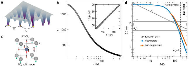
Figure 1: Electron glass, quantum paraelectricity and temperature dependence of electron’s mean free path in KTaO_3-δ a. A schematic to describe the concept of electron glass in a disordered insulator with highly localized electronic states. Here the solid colored cones represent the random disorder potential and yellow-filled circles represent electrons trapped in them. Disorder tries to make the distribution of doped carriers random, however long-range Coulomb interactions ($U_{1}$, $U_{2}$) try to make the distribution homogeneous leading to electronic frustration. b. Temperature dependent dielectric constant ($\epsilon$) of pristine (001) oriented KTaO₃ single crystal recorded at an AC frequency of 10 MHz. Sitting on the verge of quantum critical point, KTaO₃ is long known for its peculiar dielectric properties wherein the onset of quantum fluctuation leads to a marked departure from classical paraelectric behavior below 35 K leading to saturation of $\epsilon$ at low temperature. This crossover entails an interesting non-classical $T^{2}$ dependence of the inverse of $\epsilon$ below 35 K (shown in the inset) which can be taken as a sign of the onset of quantum paraelectricity [10]. c. Unit cell of pristine KTaO₃ along with the transverse optical soft mode. d. In the Drude-Boltzman picture, conductivity ($\sigma$) of metal is given by $\sigma$=$n$$e$²$\tau$/$m$^∗=$e$²($k_{F}$)²$l_{e}$/3$\pi$²$\hbar$ where $n$ is the carrier density, $\tau$ is scattering time constant, $k_{F}$ is Fermi wave vector, $m$^∗ is the effective mass of electrons and $l_{e}$ is the electron’s mean free path. $l_{e}$ calculated using this formula for a sample with $n$=5.7$\crossproduct$10¹⁷ cm^-3 has been shown by a blue curve. At such a dilute limit, the Fermi surface has little anisotropy (see our previous work  [11]), keeping this in mind $k_{F}$ has been calculated by effectively mapping the ellipsoidal Fermi surface onto a spherical Fermi surface. As evident from the plot, above $\sim$140 K, $l_{e}$ becomes shorter than the inverse of $k_{F}$ and the system enters into a bad metal phase. Further, at such dilute density and with $m$^∗=0.56 $m_{e}$ the Fermion degeneracy temperature is found to be 68 K. Above this temperature, electrons become non-degenerate and the modified $l_{e}$ is given by $l^{\prime}_{e}$$\sim$ $l_{e}$ $n$^-1/3/$\Lambda$ [12] where $\Lambda$ is the de Broglie thermal wavelength given by $\Lambda$=$h$/$\sqrt{2\pi m^{*}k_{B}T}$. The orange curve shows the calculated $l_{e}$ for the non-degenerate case. As evident, this exercise only shifts the curve to a little higher temperature, however, the conclusions remain the same.

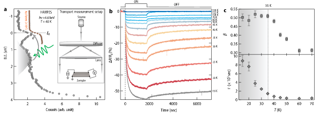
Figure 2: HAXPES and transport measurements under light a. Near Fermi level electronic states measured at 40 K using hard X-ray photoemission spectroscopy on the KTaO_3-δ sample. Binding energy was corrected by taking Au Fermi level as a reference. In the figure, Au Fermi level intensity has been reduced by thousand times and shifted rightward for comparison. Inset shows a home-built setup for transport measurement under light illumination (see methods for more details). Green arrow shows the incoming photon which excites trapped electrons to the conduction band (shown with slate-gray color). b. Temporal evolution of resistance under green light illumination ($\lambda$ = 527 nm, power = 145 $\mu$ watt) for 30 minutes measured at several fixed temperatures. After 30 minutes, resistance relaxation was observed in dark for the next 1.5 hours. For comparative analysis, change in resistance has been converted into relative percentage change ($\Delta$$R$/$R_{0}$)$\crossproduct$100. Additional measurements with red light have been shown in Supplementary Information Section 2 and Supplementary Fig. 2. c. Temperature dependence of stretching exponent ($\beta$) and relaxation time ($\tau$) obtained from fitting of resistance relaxation in light off stage with a stretched exponential function. We further emphasize that, while the value $\beta$ has been obtained by fitting the data for 1.5 hours, the same value is obtained even when the data is fitted for a longer period of up to 24 hours (Supplementary Information Section 3 and Supplementary Fig. 3).

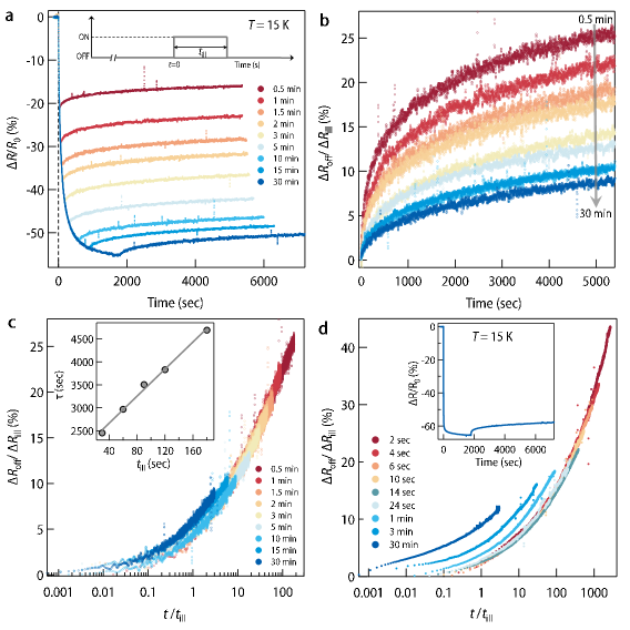
Figure 3: Aging phenomena a. Relative percentage change in resistance ($\Delta$$R$/$R_{0}$)$\crossproduct$100 measured at 15 K for different $t$${}_{\text{ill}}$ ranging from 0.5 min to 30 min. Thereafter, resistance relaxation was observed for the next 1.5 hours in every case. b. Temporal evolution of resistance relaxation in off-stage for different values of $t$${}_{\text{ill}}$. Since the amount of doping depends on the duration of light illumination, the change in resistance in the off-stage ($\Delta$$R$${}_{\text{off}}$) has been normalized with a total drop in resistance ($\Delta$$R$${}_{\text{ill}}$) at the end of illumination [19]. c. Upon re-scaling the time axis with $t$${}_{\text{ill}}$, all the curves in off-stage (except $t$${}_{\text{ill}}$ = 30 min) are found to fall on a universal curve. Inset shows the linear relationship between $\tau$ and $t$${}_{\text{ill}}$ which is the defining criteria for simple/full aging. d. Simple aging observed for another sample at 15 K. Inset shows one representative resistance relaxation data at 15 K.

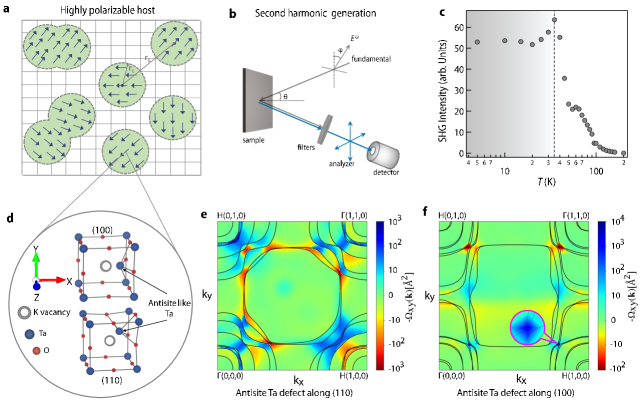
Figure 4: Polar nano regions, second harmonic generation measurement and density functional theory a. A schematic depicting real space random distribution of polar nano regions in a highly polarizable host lattice. b. A schematic of the experimental setup for measuring optical second harmonic generation signal in reflection geometry (for more details see methods section). c. Temperature-dependent SHG intensity measured on KTaO_3-δ sample. d. A portion of the relaxed structure of supercell of size 2$\crossproduct$2$\crossproduct$2 of KTaO₃ with Ta off-centering along the (100) and (110) direction around K vacancy. For more details, see the methods section and Supplementary Information Section 8 and Supplementary Fig. 8. e. Plot of Berry curvature $\Omega_{xy}(\mathbf{k})$ (shown in color-map) for $k_{z}=0$ and bands (solid contours) intersecting the Fermi surface for the system having an antisite-like Ta defect along (110) direction. f. Same as e. for the system with an antisite-like Ta defect along (100) direction. The inset shows the spin-orbit induced avoided crossing of bands yielding large contributions to the Berry curvature. We get average polarization of 5.8 $\mu C/cm^{2}$ and 11.1 $\mu C/cm^{2}$ for Ta²⁺ antisite-like defect along (110) and (100) respectively for the supercell of size $2\crossproduct 2\crossproduct 2$. We also note that, we do not observe any polarization in pristine KTaO₃.

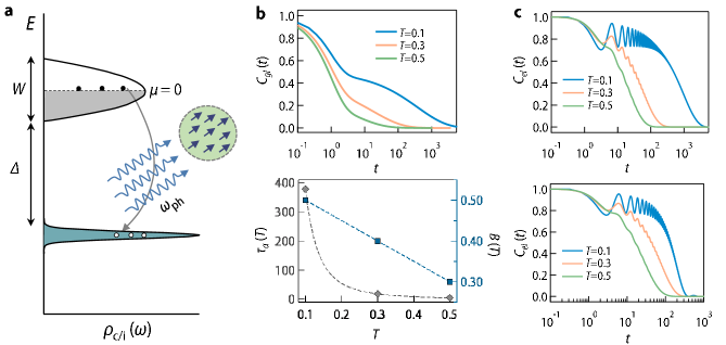
Figure 5: Theoretical calculations a. A schematic of band diagram considered for computing inter band transitions when the conduction electron is coupled to glassy background from randomly oriented polar nano regions. b. (Upper panel) The glass correlation function $C_{gl}(t)$ vs. $t$ for three temperatures for $\tau_{s}(T)=1$, $b=0.5$. (Lower panel) Plot of $\tau_{\alpha}(T)\sim T^{-2.8}$ vs. $T$ (left y axis, in units of $\tau_{s}$) and $B(T)$ (right y axis) vs. $T$ ($A=1-B$) for three temperatures. c. (upper panel) The density-density correlation function of conduction electron $C_{el}(t)$ vs. $t$ for three temperatures for flat ($W=0$) conduction band. (lower panel) $C_{el}(t)$ vs. $t$ for three temperatures for semicircular conduction band with $W=0.01$

.

Supplementary Information

List of contents

Section 1. Sheet resistance vs temperature plot.

Section 2. Experiment with red light.

Section 3. Long-time relaxation of persistence photo-resistance.

Section 4. Deviation of persistence photo-resistance relaxation time ($\tau$) from activated behavior at low temperature.

Section 5. Dielectric loss in pristine KTaO₃.

Section 6. Correspondence between the appearance of polar nano regions and photo-doping effect.

Section 7. Presence of potassium vacancy.

Section 8. Berry phase calculations.

Section 9. Toy model of complex inter-band electronic relaxation mediated by a glassy bath.

Supplementary Section 1: Sheet resistance vs temperature plot.

As depicted in Fig. 2b of the main text, shining light above 150 K does not have any noticeable effect. This observation is further supported by the plot shown in Supplementary Fig. 1, where we compare the $R_{S}$ vs $T$ curve obtained in the dark taken in the cooling run with the measurement conducted during the heating run after exposing the sample to green light (power= 145 $\mu$ Watt) for 30 minutes at 10 K. It is evident from the plot that the two curves converge around 150 K, indicating a lack of any significant photo-doping above 150 K.

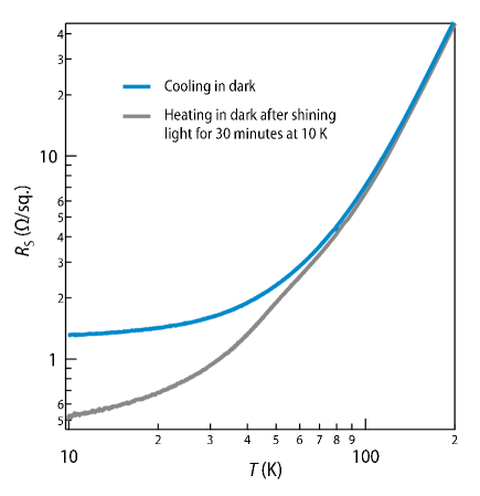
Supplementary Figure 1: Temperature dependent sheet resistance ($R$${}_{\text{S}}$) of oxygen-deficient KTaO₃ sample ($n$=5.7$\crossproduct$10¹⁷ cm^-3) taken in a cooling run in dark (sky blue curve). The slate-gray color curve shows data taken in a heating run after shining light for 30 minutes at 10 K.

Supplementary Section 2: Experiment with red light.

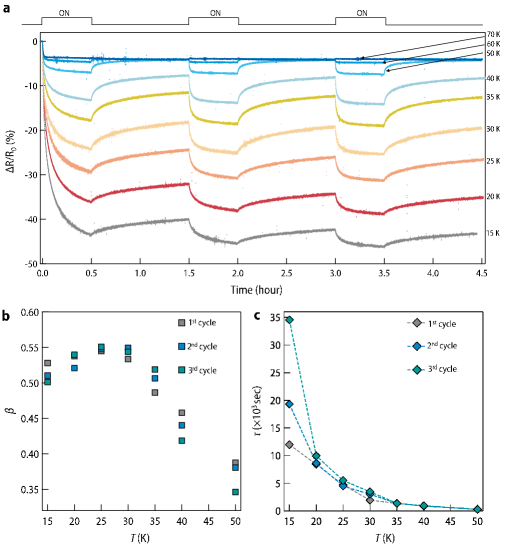
Supplementary Figure 2: a. Temporal evolution of resistance under red light illumination ($\lambda$ = 650 nm, power = 60 $\mu$ watt) for 30 minutes measured at several fixed temperatures. After 30 minutes, resistance relaxation was observed in dark for the next one hour. This measurement was repeated for 3 consecutive cycles. For comparative analysis, change in resistance has been converted into relative percentage change ($\Delta$$R$/$R_{0}$)$\crossproduct$100. b. Temperature dependence of stretching exponent ($\beta$) obtained from fitting of resistance relaxation in light off stage with a stretched exponential function for all three cycles. c. Temperature dependence of corresponding relaxation time ($\tau$) for all three cycles.

In the main text, we have presented all the measurements conducted using the green light. In this section, we provide an additional set of data obtained in three consecutive cycles (see Supplementary Fig. 2a) using a red light of wavelength $\lambda$ = 650 nm, power = 60 $\mu$ Watt). As evident from Supplementary Fig. 2b and 2c, similar to the data obtained with green light, we observe a constant value of stretching exponent ($\beta$) followed by a significant enhancement in relaxation time ($\tau$) below 35 K. This observation aligns with the findings from the measurements using green light and suggests that the behavior observed is not specific to a particular wavelength of light.

Supplementary Section 3. Long-time relaxation of persistence photo-resistance.

In Fig. 2c of the main text and Supplementary Fig. 2b, the value of the stretching exponent was determined by fitting the resistance relaxation during the off-stage, which lasted for 1.5 hours. To ensure that the resistance relaxation was substantial enough to yield a reliable fitting, we conducted an additional measurement where the resistance relaxation was observed for an entire day (see Supplementary Fig. 3). It is important to emphasize that even when the data is fitted for an extended period of up to 24 hours, the same value of $\beta$ = 0.5 is obtained.

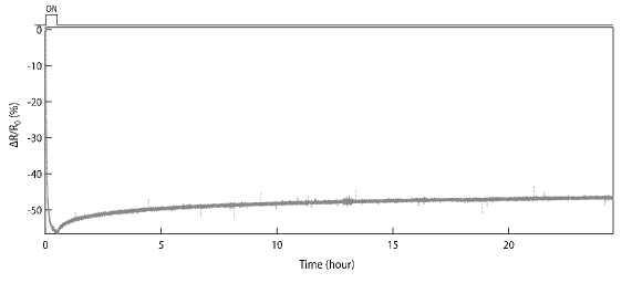
Supplementary Figure 3: Temporal evolution of resistance under green light illumination ($\lambda$ = 527 nm, power = 145 $\mu$ Watt) for 30 minutes measured at 15 K. After 30 minutes, resistance relaxation was observed in dark for the next 24 hours. For comparative analysis, change in resistance has been converted into relative percentage change ($\Delta$$R$/$R_{0}$)$\crossproduct$100.

Supplementary Section 4. Deviation of persistence photo-resistance relaxation time ($\tau$) from activated behavior at low temperature.

In the large lattice relaxation (LLR) model, the recombination of electron-hole pairs occurs through the thermal excitation of electrons over an energy barrier. This process is an activated process of the Arrhenius type. To validate this model, we have plotted ln $\tau$ against 1000/$T$ in Supplementary Fig. 4. It is evident from the plot that the data does not exhibit the expected linear behavior at low temperatures signifying that the LLR model can not account for our experimental observations.

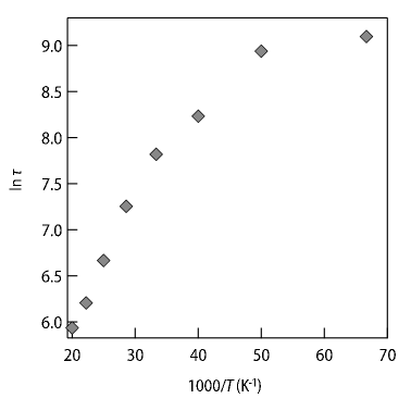
Supplementary Figure 4: Arrhenius plot of photo-resistance relaxation time ($\tau$). As evident, a clear deviation from activation behavior is observed below 35 K.

Supplementary Section 5. Dielectric loss in pristine KTaO₃.

In its ideal form, KTaO₃ is perfectly centrosymmetric and hence, should not possess any electric dipole moment. However, the presence of impurities and disorder can disrupt the crystal’s inversion symmetry, leading to the development of permanent electric dipoles [1, 2, 3, 4, 5]. In highly polarizable host such as KTaO₃, these dipoles polarize the surrounding lattice leading to formation of polar nano regions (PNRs) [6]. Under an applied AC electric field, these PNRs act as a source of dielectric losses, which can be observed as a peak in the loss tangent (tan $\delta$ = $\epsilon$${}^{{}^{\prime\prime}}$/$\epsilon$${}^{{}^{\prime}}$, where $\epsilon$${}^{{}^{\prime}}$ and $\epsilon$${}^{{}^{\prime\prime}}$ are the real and imaginary parts of the complex dielectric function, respectively).

Our temperature-dependent measurement of dielectric function indeed reveals the presence of PNRs even in our pristine KTaO₃ single crystal (see inset of Supplementary Fig. 5). Further, frequency-dependent measurements reveal that the dielectric loss is an activated process emphasizing that the PNRs in pristine crystals are very dilute and independent and hence their relaxation can be approximated by a single Debye-like process.

Supplementary Figure 5: Arrhenius plot of dielectric relaxation frequency ($f$) for pristine KTaO₃. Inset shows the dielectric loss tangent (tan $\delta$) around 54 K at $f$ = 50 kHz.

Supplementary Section 6. Correspondence between the appearance of polar nano regions and photo-doping effect.

In order to study the correlation between PNRs and photo-doping effect, we have compared the temperature-dependent total SHG intensity with the fraction of resistance (in terms of relative percentage change ($\Delta$$R$/$R_{0}$)$\crossproduct$100) which has not been recovered at the end of 1.5 hours after turning off the light. We call this quantity the persistence photo resistance denoted with the symbol $\delta$. See the inset of the bottom panel of Supplementary Fig. 6 for the definition of $\delta$. As evident, the appearance of finite signal in SHG exactly coincides with the $\delta$, strongly signifying the direct role of PNRs behind the effective electron-hole separation of our samples.

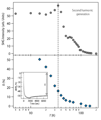
Supplementary Figure 6: (upper panel) Temperature-dependent SHG intensity measured on oxygen deficient KTaO₃ sample. (lower panel) Temperature dependence of persistence photo resistance ($\delta$) in terms of relative percentage change at the end of 1.5 hours after turning off the light (see the inset of the lower panel for the definition of $\delta$).

Supplementary Section 7. Presence of potassium vacancy.

To investigate the presence of potassium vacancy in our oxygen-deficient KTaO₃ sample, K 2p core levels were collected at the Hard X-ray Photoemission Spectroscopy (HAXPES) beamline (P22) at PETRA III, DESY. Supplementary Fig. 7a shows one representative experimental data (recorded with an incident photon energy of 5800 eV at room temperature) along with its fitting with the convolution of Lorentzian and Gaussian functions. It is evident from the figure that, in addition to the K 2p 3/2 peak at 292.65 eV arising from the lattice, there is an extra peak appearing at 293.1 eV. It has been previously shown that the presence of an additional peak at a higher binding energy is a characteristic feature of a potassium vacancy in the system [7]. In order to further understand the potassium vacancy profile in our sample, we have carried out measurements with varying photon energy from 3500 eV to 5800 eV (see Table I for the values of mean free path (MFP) and mean escape depth (MED)). As evident from Supplementary Fig. 7b, there are hardly any significant alterations in the line shape of the spectra as the photon energy was increased. This observation indicates that the potassium vacancy profile is homogeneous throughout the bulk of the sample.

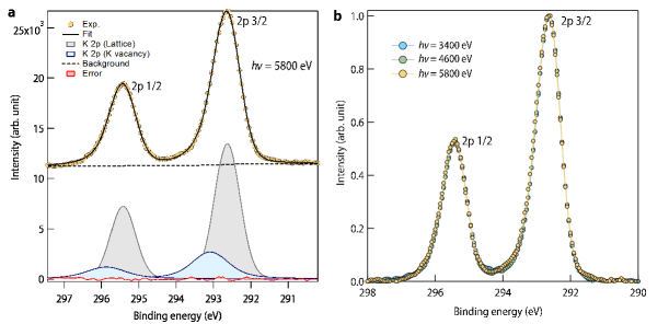
Supplementary Figure 7: a Deconvolution of K2p core level spectrum (for oxygen-deficient KTaO₃ sample) by using the convolution of Lorentzian and Gaussian function. This data was recorded at room temperature with photon energy $h$$\nu$ = 5800 eV. Yellow-filled circles denote the experimental data and a solid black line denotes the simulated spectra. Curves filled with gray and sky blue color correspond to the lattice potassium and potassium vacancy respectively. The dashed black line denotes the Shirley background and the red-filled curve corresponds to the difference between the experimental data and simulated spectra. b K 2p core level spectra recorded with varying incident photon energy. All the spectra were recorded at room temperature.

Photon energy (eV)	MFP (nm)	MED (nm)
3400	5.1	15.3
4600	6.4	19.2
5800	7.7	23.1

Table 1: Table of mean free path (MFP) and mean escape depth (MED) with increasing photon energy. MFP was calculated from the formula $m$(K.E.)^γ where K.E. is the kinetic energy of the ejected electrons and the values of $m$ and $\gamma$ were taken to be 0.12 and 0.75 respectively [8]. Further, MED was roughly assumed to be 3 times MFP which would roughly account for 95 percent of the total collected intensity.

Supplementary Section 8. Berry phase calculations.

We have investigated the probable mechanism for the realization of PNRs theoretically using noncollinear density functional (DFT) theory. Antisite defect in perovskite materials like SrTiO₃ (STO) and complex perovskite oxides (Ca, Sr)₃Mn₂O₇ is known for causing macroscopic polarization in the system [9, 10]. Due to the similarities in the electronic properties of STO and KTO, we expect KTO to develop polarization due to antsite defects. We have created Ta antisite defect in a supercell of size $2\crossproduct 2\crossproduct 2$ conventional unit cell. In our calculations, the Ta off-centering is considered along (100) and (110) directions. The relaxed structures are shown in Supplementary Fig. 8a. In Supplementary Fig. 8b we have shown the band structure of the system with Ta antisite defect along (110). The red solid lines are the bands calculated using DFT within PBE-GGA[11]. In order to calculate the macroscopic polarization in the system, we use the modern theory of polarization. The change in electronic contribution to the polarization $\Delta P$ is defined as [12, 13]

$$\Delta P=-\dfrac{e}{2\pi}\phi$$ (2)

where $\phi$ is the Berry phase, which is the integral of the Berry curvature over a surface $S$ bounded by a closed path in $k-$space, i.e., [14]

$$\phi=\int_{S}\Omega(\mathbf{k})d\mathbf{k}$$ (3)

One can calculate Berry curvature using Bloch states $u_{n}(\mathbf{k})$ as

$$\Omega_{\alpha\beta}(\mathbf{k})=\sum_{n}f_{n}(\mathbf{k})\Omega_{n,\alpha\beta}(\mathbf{k})=\sum_{n}-2f_{n}(\mathbf{k})\text{Im}\innerproduct{\partialderivative{u_{n}(\mathbf{k})}{k_{\alpha}}}{\partialderivative{u_{n}(\mathbf{k})}{k_{\beta}}}$$ (4)

where $\alpha,\beta$ are the cartesian indices and $f_{n}(\mathbf{k})$ is the occupation number of the state $n$. Ta antisite defects in KTO have a partially occupied band. As it well known, taking derivatives of $u_{n}(\mathbf{k})$ in a finite-difference scheme in the presence of band crossing and avoided crossing becomes difficult. We followed the procedure described by X. Wang et. al. [15] for the calculation of Berry curvature using Wannier functions as implemented in the Wannier90 code [16]. In Supplementary Fig. 8b, we have shown the Wannier interpolated bands in black dotted lines. From the figure, it is clear that both the set of bands calculated using DFT and Wannier interpolation match very well near the Fermi level. In Supplementary Fig. 8c, we have shown the total Berry curvature for the antisite Ta defect along (110) in the plane $k_{z}=0$ calculated using 2D k-mesh of size $41\crossproduct 41$ (top panel) and $101\crossproduct 101$ (bottom panel). While there are small quantitative differences, the qualitative features in both the panels remain the same.

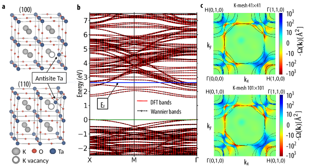
Supplementary Figure 8: a. The relaxed structure of KTaO₃ (KTO) with Ta off-centering along the (100) and (110) direction around K vacancy (antisitelike Ta defect) for a supercell of size 2$\crossproduct$2$\crossproduct$2. b. Bandstructure plot for (110) direction antisitelike Ta defect calculated using density functional theory within PBE-GGA (shown in red solid lines) and Wannier interpolated bands (shown in black dotted lines). The blue solid line is the Fermi energy. c. Plot of total Berry curvature in the plane $k_{z}=0$ (in log scale) for the (110) antisitelike Ta defect structure calculated on a 2D k-mesh of sample-size $41\crossproduct 41$ (top panel) and $101\crossproduct 101$ (bottom panel).

Supplementary Section 9. Toy model of complex inter-band electronic relaxation mediated by a glassy bath.

As discussed in the main text, we consider the following model of coupled electron (el)-glass (gl) system.

$$H =H_{el}+H_{gl}+H_{el-gl}$$ (5a)

$$H_{el} =-\sum_{i,j=1}^{N_{c}}t_{ij}c_{i}^{\dagger}c_{j}-\varepsilon_{0}\sum_{\alpha=1}^{N_{f}}f_{\alpha}^{\dagger}f_{\alpha},~{}~{}~{}~{}(\varepsilon_{0}>0)$$ (5b)

$$H_{gl} =\sum_{\mu=1}^{N_{g}}\frac{p_{\mu}^{2}}{2m}+U(\{x_{\mu}\})$$ (5c)

$$H_{el-gl} =\sum_{i\alpha\mu}(V_{i\alpha\mu}c_{i}^{\dagger}f_{\alpha}+\mathrm{h.c.})x_{\mu}$$ (5d)

The electronic part consists of a conduction band and a flat impurity band at energy $-\varepsilon_{0}$. We consider three different energy dispersions for the conduction band, corresponding to different lattices and hopping amplitudes $t_{ij}$, namely – (1) a flat band or $\delta$ function density of states (DOS) with bandwidth $W=0$, (2) a semicircular DOS, $g(\epsilon)=(1/2\pi)\sqrt{W^{2}-\omega^{2}}\theta(W-|\omega|)$ with band width $W$ [$\theta(x)$ is heaviside step function], e.g., corresponding to a Bethe lattice, and (3) DOS corresponding to three-dimensional (3d) simple cubic lattice with nearest-neighbour hopping $W/12$. The band gap between the conduction band minimum and the impurity band is $\Delta=\varepsilon_{0}-W/2$. We set the chemical potential at the center of the conduction band, i.e., $\mu=0$, as appropriate for a metallic system (see Fig. 5(a) of main text).

The Hamiltonian $H_{gl}$ for a set of particles with positions $\{x_{\mu}\}$, and their canonically conjugate momenta $p_{\mu}$ ($[x_{\mu},p_{\nu}]=\imath\delta_{\mu\nu}$ with $\hbar=1$) models the dynamics of a local glassy background. The exact form of the inter-particle interaction $U(\{x_{\mu}\})$ is not crucial for our calculations. However, as an example, we take $U(\{x_{\mu}\})=\sum_{\mu<\nu<\gamma}J_{\mu\nu\gamma}x_{\mu}x_{\nu}x_{\gamma}$ with the spherical constraint $\sum_{\mu}x_{\mu}^{2}=N_{g}$, corresponding a well-known solvable model for glasses, namely the infinite-range spherical $p$-spin glass model with $p=3$-spin coupling [17]. Here, $J_{\mu\nu\gamma}$ is real Gaussian random number with zero mean and variance $\overline{J^{2}_{\mu\nu\gamma}}=3!J^{2}/2N_{g}^{2}$, where the overline denotes averaging over different realizations of $J_{\mu\nu\gamma}$. The particular scaling with $N_{g}$ ensures extensive free energy in the thermodynamic limit $N_{g}\to\infty$. The $p$-spin glass model, with both quantum [17] and classical dissipative [18] dynamics, undergoes a glass transition at temperature $T_{g}\sim J$. For temperature $T\gtrsim T_{g}$, the model gives rise to a supercooled liquid regime, like standard structural glasses [19], with complex two-step relaxation for the dynamical correlation function

$$C_{gl}(t) =\overline{\langle x_{\mu}(t)x_{\mu}(0)\rangle}=Ae^{-|t|/\tau_{s}}+Be^{-(|t|/\tau_{\alpha})^{\beta}}$$ (6)

, having a short-time exponential decay, and long-time stretched exponential decay.

To obtain a solvable model for the coupled el-gl system, we also take the coupling $V_{i\alpha\mu}$ between the glass, and the conduction and impurity electronic states, infinite range. Here $V_{i\alpha\mu}$ is a complex Gaussian random number with zero mean and variance $\overline{|V_{i\alpha\mu}|^{2}}=V/(N_{c}N_{f}N_{g})^{1/3}$. The particular scaling ensures a well-defined thermodynamic limit $N_{c},N_{f},N_{g}\to\infty$ with finite ratios $p_{f}=N_{f}/N_{c}$ and $p_{g}=N_{g}/N_{c}$. The ratios allow us tune the backaction of one part of the system on the other. For example, for simplicity, and to gain an analytical understanding, as discussed below, we take $p_{f},p_{g}\gg 1$, such that the back actions of the conduction electrons on the impurity electrons and the glass are negligible. We expect our main conclusions to be valid for $p_{f},p_{g}\approx 1$, i.e., when the backaction is substantial.

For the above-disordered model (Supplementary Eq. (5)), using the standard replica method [20, 17], we calculate the disorder-averaged connected equilibrium dynamical density-density correlation function for the conduction electrons, $C_{el}(t)=\overline{\langle n_{i}(t)n_{i}(0)\rangle}-\langle n_{i}(0)\rangle^{2}$, at temperature $T\ll\Delta$. Here $n_{i}=c_{i}^{\dagger}c_{i}$ is the conduction electron density. The correlation function $C_{el}(t)$ captures the relaxation of the thermally excited electrons in the conduction band at a finite temperature.

We obtain the replicated partition function, $Z^{n}=\int\mathcal{D}(\bar{c},c)\mathcal{D}(\bar{f},f)\mathcal{D}x\exp(-S[\bar{c},c,\bar{f},f,x])$, as coherent-state imaginary-time path integral over the fermionic Grassmann fields $\{\bar{c}_{ia},c_{ia},\bar{f}_{\alpha a},f_{\alpha a}\}$ and position variables $\{x_{ia}\}$, with replica index $a=1,\cdots,n$ and the action,

$$S_{n} =\int_{0}^{1/T}d\tau\sum_{ij,a}\bar{c}_{ia}(\tau)[(\partial_{\tau}-\mu)\delta_{ij}-t_{ij}]c_{ja}(\tau)+\int_{0}^{1/T}d\tau\sum_{\alpha,a}\bar{f}_{\alpha a}(\tau)(\partial_{\tau}-\mu-\varepsilon_{0})f_{\alpha a}(\tau)$$

$$+\int_{0}^{1/T}d\tau\bigg{[}\frac{1}{2}\sum_{\mu,a}[m({\partial_{\tau}x_{\mu a}})^{2}+zx_{\mu a}^{2}]+\sum_{\mu\nu\gamma,a}J_{\mu\nu\gamma}x_{\mu a}(\tau)x_{\nu a}(\tau)x_{\gamma a}(\tau)\bigg{]}$$

$$+\int_{0}^{1/T}d\tau\sum_{i\alpha\mu,a}[V_{i\alpha\mu}\bar{c}_{ia}(\tau)f_{\alpha a}(\tau)x_{\mu a}(\tau)+\mathrm{h.c.}],$$ (7)

where the Lagrange’s multiplier $z(\tau)$ imposes the spherical constraint on $x_{\mu a}(\tau)$. After averaging over the distributions of $J_{\mu\nu\gamma}$ and $V_{i\alpha\mu}$, we obtain $\overline{Z^{n}}$ and the corresponding action as

$$\tilde{S}_{n} =\int_{0}^{1/T}d\tau\sum_{ij,a}\bar{c}_{ia}(\tau)[(\partial_{\tau}-\mu)\delta_{ij}-t_{ij}]c_{ja}(\tau)+\int_{0}^{1/T}d\tau\sum_{\alpha,a}\bar{f}_{\alpha a}(\tau)(\partial_{\tau}-\mu-\varepsilon_{0})f_{\alpha a}(\tau)$$

$$+\frac{1}{2}\int^{1/T}_{0}d\tau\sum_{\mu a}x_{\mu a}(\tau)(-m\partial^{2}_{\tau}+z)x_{\mu a}(\tau)+N_{c}\int d\tau d\tau^{\prime}\sum_{ab}\bigg{[}V^{2}(p_{f}p_{g})^{1/3}G_{ab}(\tau,\tau^{\prime})\mathcal{G}_{ba}(\tau^{\prime},\tau)Q_{ab}(\tau,\tau^{\prime})$$

$$-\frac{J^{2}p_{g}}{4}Q^{3}_{ab}(\tau,\tau^{\prime})\bigg{]},$$ (8)

where we have introduced the large $N$-fields,

$$G_{ab}(\tau,\tau^{\prime}) =-\frac{1}{N_{c}}\sum_{i}c_{ia}(\tau)\bar{c}_{ib}(\tau^{\prime})$$ (9a)

$$\mathcal{G}_{ab}(\tau,\tau^{\prime}) =-\frac{1}{N_{f}}\sum_{\alpha}f_{\alpha a}(\tau)\bar{f}_{\alpha b}(\tau^{\prime})$$ (9b)

$$Q_{ab}(\tau,\tau^{\prime}) =\frac{1}{N_{g}}\sum_{\mu}x_{\mu a}(\tau)x_{\mu b}(\tau^{\prime})$$ (9c)

To promote the above as fluctuating dynamical fields, conjugate fields $\Sigma_{ba}(\tau^{\prime},\tau)$, $\sigma_{ba}(\tau^{\prime},\tau)$ and $\Pi_{ab}(\tau,\tau^{\prime})$ are introduced for $G,~{}\mathcal{G}$ and $Q$, respectively, e.g., by using the relation

$$\int\mathcal{D}G\prod_{a\tau,b\tau^{\prime}}\delta(N_{c}G_{ab}(\tau,\tau^{\prime})+\sum_{i}c_{ia}(\tau)\bar{c}_{ib}(\tau^{\prime}))=\int\mathcal{D}G\mathcal{D}\Sigma e^{-\int d\tau d\tau^{\prime}\Sigma_{ba}(\tau^{\prime},\tau)[N_{c}G_{ab}(\tau,\tau^{\prime})+\sum_{i}c_{ia}(\tau)\bar{c}_{ib}(\tau^{\prime})]}=1$$ (10)

As a result, we can now integrate out the fields $(\bar{c},c)$, $(\bar{f},f)$, and $x$. Assuming replica diagonal ansatz, e.g., $G_{ab}(\tau,\tau^{\prime})=\delta_{ab}G(\tau,\tau^{\prime})$, we obtain $\overline{Z^{n}}=\int\mathcal{D}(G,\mathcal{G},Q,\Sigma,\sigma,\Pi)e^{-nS_{eff}}$ and the effective action

$$S_{\rm eff} =-N_{c}\int d\epsilon g(\epsilon)\Tr\ln\big(-\partial_{\tau}+\mu-\epsilon-\Sigma\big{missing})-N_{f}\Tr\ln\big(-\partial_{\tau}+\mu+\varepsilon_{0}-\sigma\big{missing})+$$

$$\frac{N_{g}}{2}\Tr\ln\big(-m\partial^{2}_{\tau}+z-\Pi\big{missing})-N_{c}\int d\tau d\tau^{\prime}\big{[}\Sigma(\tau,\tau^{\prime})G(\tau^{\prime},\tau)+p_{f}\sigma(\tau,\tau^{\prime})\mathcal{G}(\tau^{\prime},\tau)+\frac{p_{g}J^{2}}{4}Q(\tau,\tau^{\prime})^{3}$$

$$-\frac{p_{g}}{2}\Pi(\tau,\tau^{\prime})Q(\tau^{\prime},\tau)-V^{2}(p_{f}p_{g})^{1/3}G(\tau,\tau^{\prime})\mathcal{G}(\tau^{\prime},\tau)Q(\tau,\tau^{\prime})\big{]}$$ (11)

In the large $N_{c}$ limit, the saddle point solution is obtained by varying the above action with respect to $G,\Sigma,\mathcal{G},\sigma,Q,\Pi$ and setting the variations to zero. Due to time-translation invariance at equilibrium, e.g., $G(\tau,\tau^{\prime})=G(\tau-\tau^{\prime})$ and $z(\tau)=z$. As a result, we can write the saddle point equations in the following form after performing a Matsubara Fourier transform first, e.g., $G(\tau-\tau^{\prime})\to G(\imath\omega_{n})$ with fermionic Matsubara frequency $\omega_{n}$, and then doing an analytical continuation, $G(\imath\omega_{n})\to G_{R}(\omega+\imath 0^{+}$), to real frequencies, where $G_{R}$ is the retarded Green’s function.

$$G_{R}(\omega) =\int d\epsilon g(\epsilon)\frac{1}{\omega+\mu-\epsilon-\Sigma_{R}(\omega)}$$ (12a)

$$\mathcal{G}_{R}^{-1}(\omega) =\omega+\mu+\varepsilon_{0}-\sigma_{R}(\omega)$$ (12b)

$$Q_{R}^{-1}(\omega) =-m\omega^{2}+z-\Pi_{R}(\omega)$$ (12c)

$$\Sigma(\tau) =V^{2}(p_{f}p_{g})^{1/3}\mathcal{G}(\tau)Q(\tau)$$ (12d)

$$\sigma(\tau) =V^{2}p_{g}^{1/3}p_{f}^{-2/3}G(\tau)Q(\tau)$$ (12e)

$$\Pi(\tau) =\frac{3J^{2}}{2}Q^{3}(\tau)+V^{2}p_{f}^{1/3}p_{g}^{-2/3}G(\tau)\mathcal{G}(-\tau)$$ (12f)

In the limit $p_{f},p_{g}\gg 1$, we can approximate $\sigma(\tau)\approx 0$ and $\Pi(\tau)\approx(3J^{2}/2)Q^{3}(\tau)$, and neglect the back action of the conduction electrons on the impurity states and the glass.

In this limit, following the numerical procedure similar to that in reference [21, 22], we can numerically solve the above self-consistency equations for various conduction electron DOS $g(\epsilon)$ to obtain the retarded functions $G_{R}(\omega)$ and $Q_{R}(\omega)$, whereas the retarded Green’s function of the impurity band is given by $\mathcal{G}_{R}(\omega)=(\omega+\imath 0^{+}+\mu+\varepsilon_{0})^{-1}$. However, instead of self-consistently solving for $Q_{R}(\omega)$, we use the Supplementary Eq. (6) to obtain the spectral function of the glass from the fluctuation-dissipation relation

$$\rho_{gl}(\omega) =-\frac{1}{\pi}\mathrm{Im}Q_{R}(\omega)=-\frac{1}{\pi}\tanh\left(\frac{\omega}{2T}\right)C_{gl}(\omega),$$ (13)

where $C_{gl}(\omega)=\int_{-\infty}^{\infty}dte^{\imath\omega t}C_{gl}(t)$. As a result, the conduction electron self-energy can be obtained as

$$\Sigma_{R}(\omega) =V^{2}\int d\omega_{1}d\omega_{2}\rho_{f}(\omega_{1})\rho_{gl}(\omega_{2})\frac{n_{F}(\omega_{1})n_{B}(\omega_{2})-n_{F}(-\omega_{1})n_{B}(-\omega_{2})}{\omega-\omega_{1}-\omega_{2}+\imath 0^{+}},$$ (14)

where $n_{F}(\omega)$ and $n_{B}(\omega)$ are Fermi and Bose functions, respectively, and $\rho_{f}(\omega)=\delta(\omega+\varepsilon_{0})$ is the spectral function of the impurity electrons. Here we have redefined $V^{2}(p_{f}p_{g})^{1/3}$ as $V^{2}$. Thus, using $\Sigma_{R}(\omega)$ in Supplementary Eq. (12a), we can obtain the conduction electron Green’s function $G_{R}(\omega)$.

.1 Density density correlation function

To capture the manifestation of the glassy relaxation in the electron-hole recombination process we look into the connected density-density correlator $C_{el}(t)=\langle n_{i}(t)n_{i}(0)\rangle-\langle n_{i}(0)\rangle^{2}$, which captures the relaxation of the thermally excited carriers at temperature $T$. $C_{el}(t)$ can be obtained from the imaginary-time correlation function $C_{el}(\tau)=\langle n(\tau)n(0)\rangle-\langle n(0)\rangle^{2}$, where $n(\tau)=(1/N_{c})\sum_{i}c^{\dagger}_{i}(\tau)c(\tau)$. In the large-$N_{c}$ limit, the connected correlator is given by the bubble diagram and can be expressed as $C_{el}(\tau)=G(\tau)G(-\tau)$. Performing Matsubara Fourier transformation and then analytically continuing $i\Omega_{n}\to\omega+i0^{+}$, where $\Omega_{m}$ is bosonic Matsubara frequency, we can obtain the retarded correlator

$$C_{el,R}(\omega)=\int d\omega_{1}d\omega_{2}\rho_{c}(\omega_{1})\rho_{c}(\omega_{2})\bigg{(}\frac{n_{F}(\omega_{1})n_{F}(-\omega_{2})-n_{F}(-\omega_{1})n_{F}(\omega_{2})}{\omega_{1}-\omega_{2}-\omega_{n}-i0^{+}}\bigg{)},$$ (15)

where $\rho_{c}(\omega)=-(1/\pi)\mathrm{Im}G_{R}(\omega)$ is the conduction electron spectral function. Using the fluctuation-dissipation theorem, we can relate $C_{el,R}(\omega)$ to the Fourier transform of the real-time density-density correlation function $C_{el}(t)$ as $C_{el}(\omega)=\coth(\omega/2T)\text{Im}C_{el,R}(\omega)$. Finally, performing the inverse Fourier transform we obtain the real-time density-density correlation function $C_{el}(t)=\int^{\infty}_{-\infty}(d\omega/2\pi)e^{-i\omega t}C_{el}(\omega)$. We show the results for the numerically computed $C_{el}(t)$ in Fig. 5(c) of the main text for (1) a flat conduction band ($W=0$), and (2) a semicircular conduction band DOS, using $C_{gl}(t)$ from Supplementary Eq. (6) (Fig. 5(b), main text). For the latter, we take a temperature-independent stretching exponent $\beta=0.5$ and the $\alpha$-relaxation time $\tau_{\alpha}(T)$, which varies as $\sim T^{-2.8}$, consistent with our experimental results (Fig. 2(c), main text). We also vary the coefficient $B(T)\leq 1$ such that it increases with decreasing temperature, while $A(T)=1-B(T)$. This leads to a more dominant long-time stretched exponential part in $C_{gl}(t)$ at lower temperatures, compared to the short-time exponential decay in Supplementary Eq. (6). In Supplementary Fig. 9, we show the results for the conduction band energy dispersion corresponding to a nearest-neighbour tight binding model on a simple cubic lattice. We can see that in all the cases the glassy relaxation of the bath influences the relaxation of the conduction electrons leading complex and temperature dependent relaxation profile for $C_{el}(t)$.

We can obtain a simple analytical understanding of the above results as follows. From Supplementary Eq. (14), we can obtain for $\mu=0$

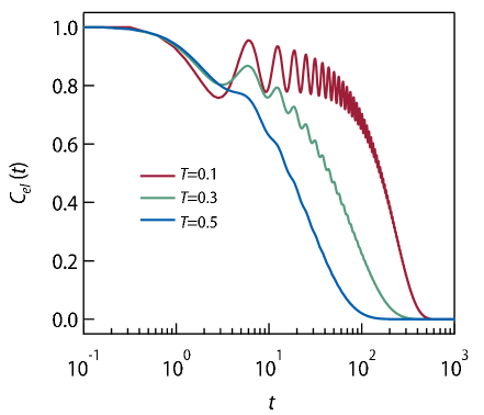
Supplementary Figure 9: The density-density correlation function of conduction electron $C_{el}(t)$ vs. $t$ for three temperatures corresponding to a nearest-neighbour tight binding model on a simple cubic lattice

$$\gamma(\omega)={\rm Im}\Sigma_{R}(\omega) =-\pi V^{2}\rho_{gl}(\omega+\varepsilon_{0})\big{(}n_{F}(-\varepsilon_{0})+n_{B}(-\varepsilon_{0}-\omega)\big{)}$$ (16)

Thus, by defining $k(\omega)=\mathrm{Re}\Sigma_{R}(\omega)$, we obtain from Eq.(12a)

$${\rm Im}G_{R}(\omega) =\int d\epsilon g(\epsilon)\frac{\gamma(\omega)}{(\omega-\epsilon-k(\omega))^{2}+\gamma(\omega)^{2}}$$ (17)

As a result, from Supplementary Eq. (15) we get

$${\rm Im}C_{el,R}(\omega) =\int d\omega_{1}\rho_{c}(\omega_{1})\rho_{c}(\omega_{1}-\omega)\big{(}n_{F}(\omega_{1})-n_{F}(\omega_{1}-\omega)\big{)}$$ (18)

The above can be expressed as

$${\rm Im}C_{R}(\omega) =\frac{1}{\pi^{2}}\int d\epsilon_{1}d\epsilon_{2}g(\epsilon_{1})g(\epsilon_{2})\int d\omega_{1}\bigg{[}\frac{\gamma(\omega_{1})}{(\omega_{1}-\epsilon_{1}-k(\omega_{1}))^{2}+\gamma(\omega_{1})^{2}}$$

$$\frac{\gamma(\omega_{1}-\omega)}{(\omega_{1}-\omega-\epsilon_{2}-k(\omega_{1}-\omega))^{2}+\gamma(\omega_{1}-\omega)^{2}}\bigg{]}\big{(}n_{F}(\omega_{1})-n_{F}(\omega_{1}-\omega)\big{)}$$ (19)

Thus,

$$C_{el}(t)=\int_{-\infty}^{\infty}d\omega_{1}d\omega e^{-\imath\omega t}\rho_{gl}(\omega_{1}+\varepsilon_{0})\rho_{gl}(\omega_{1}+\varepsilon_{0}-\omega)F(\omega,\omega_{1})$$ (20)

can be written as a convolution over the glass spectral function $\rho_{gl}(\omega)$, where

$$F(\omega,\omega_{1}) =\frac{V^{4}}{2\pi}\int d\epsilon_{1}d\epsilon_{2}\frac{g(\epsilon_{1})g(\epsilon_{2})\coth\left(\omega/2T\right)[n_{F}(\omega_{1})-n_{F}(\omega_{1}-\omega)]}{[(\omega_{1}-\epsilon_{1}-k(\omega_{1}))^{2}+\gamma(\omega_{1})^{2}][(\omega_{1}-\omega-\epsilon_{2}-k(\omega_{1}-\omega))^{2}+\gamma(\omega_{1}-\omega)^{2}]}$$

$$\big{(}n_{F}(-\varepsilon_{0})+n_{B}(-\varepsilon_{0}-\omega_{1})\big{)}\big{(}n_{F}(-\varepsilon_{0})+n_{B}(-\varepsilon_{0}-\omega_{1}+\omega)\big{)}$$ (21)

The spectral function of the glass contains the information about the multiple time scales and the non-trivial temperature dependence of the glassy relaxation. Thus if appropriate conditions on the electronic energy scales $W$ and $\varepsilon_{0}$ ($\Delta$) are made relative to the energy scales of the glass, e.g., $\tau_{s}^{-1}$ and $\tau_{\alpha}^{-1}$, then the complex relaxation of the conduction electrons can be obtained. We numerically find that these conditions are met if the glassy bath is broad, i.e., the bandwidth of the glass is comparable or larger than the electronic energy scales.

References

- [1] Davies, J. H., Lee, P. A. & Rice, T. M. Electron glass. Phys. Rev. Lett. 49, 758–761 (1982). URL https://link.aps.org/doi/10.1103/PhysRevLett.49.758.
- [2] Anderson, P. W. Absence of diffusion in certain random lattices. Phys. Rev. 109, 1492–1505 (1958). URL https://link.aps.org/doi/10.1103/PhysRev.109.1492.
- [3] Dobrosavljevic, V., Trivedi, N. & Valles Jr, J. M. Conductor insulator quantum phase transitions (Oxford University Press, 2012).
- [4] Pollak, M., Ortuño, M. & Frydman, A. The electron glass (Cambridge University Press, 2013).
- [5] Amir, A., Oreg, Y. & Imry, Y. Electron glass dynamics. Annual Review of Condensed Matter Physics 2, 235–262 (2011). URL https://doi.org/10.1146/annurev-conmatphys-062910-140455.
- [6] Kar, S., Raychaudhuri, A. K., Ghosh, A., Löhneysen, H. v. & Weiss, G. Observation of non-gaussian conductance fluctuations at low temperatures in si:p(b) at the metal-insulator transition. Phys. Rev. Lett. 91, 216603 (2003). URL https://link.aps.org/doi/10.1103/PhysRevLett.91.216603.
- [7] Mahmood, F., Chaudhuri, D., Gopalakrishnan, S., Nandkishore, R. & Armitage, N. P. Observation of a marginal fermi glass. Nature Physics 17, 627–631 (2021). URL https://doi.org/10.1038/s41567-020-01149-0.
- [8] Pastor, A. A. & Dobrosavljević, V. Melting of the electron glass. Phys. Rev. Lett. 83, 4642–4645 (1999). URL https://link.aps.org/doi/10.1103/PhysRevLett.83.4642.
- [9] Markland, T. E. et al. Quantum fluctuations can promote or inhibit glass formation. Nature Physics 7, 134–137 (2011). URL https://doi.org/10.1038/nphys1865.
- [10] Rowley, S. E. et al. Ferroelectric quantum criticality. Nature Physics 10, 367–372 (2014). URL https://doi.org/10.1038/nphys2924.
- [11] Ojha, S. K. et al. Oxygen vacancy-induced topological hall effect in a nonmagnetic band insulator. Advanced Quantum Technologies 3, 2000021 (2020). URL https://doi.org/10.1002/qute.202000021.
- [12] Lin, X. et al. Metallicity without quasi-particles in room-temperature strontium titanate. npj Quantum Materials 2, 41 (2017). URL https://doi.org/10.1038/s41535-017-0044-5.
- [13] Chandra, P., Lonzarich, G. G., Rowley, S. E. & Scott, J. F. Prospects and applications near ferroelectric quantum phase transitions: a key issues review. Reports on Progress in Physics 80, 112502 (2017). URL https://doi.org/10.1088/1361-6633/aa82d2.
- [14] Gupta, A. et al. Ktao3—the new kid on the spintronics block. Advanced Materials 34, 2106481 (2022). URL https://doi.org/10.1002/adma.202106481.
- [15] Changjiang, L. et al. Two-dimensional superconductivity and anisotropic transport at ktao3 (111) interfaces. Science 371, 716–721 (2021). URL https://doi.org/10.1126/science.aba5511.
- [16] Ren, T. et al. Two-dimensional superconductivity at the surfaces of ktao3 gated with ionic liquid. Science Advances 8, eabn4273 (XXXX). URL https://doi.org/10.1126/sciadv.abn4273.
- [17] Ojha, S. K., Mandal, P., Kumar, S. & Middey, S. Anomalous dissipation in ktao (111) interface superconductor in the absence of external magnetic field. arXiv preprint arXiv:2206.10361 (2022).
- [18] Ojha, S. K. et al. Oxygen vacancy induced electronic structure modification of . Phys. Rev. B 103, 085120 (2021). URL https://link.aps.org/doi/10.1103/PhysRevB.103.085120.
- [19] Lee, M. et al. The electron glass in a switchable mirror: relaxation, ageing and universality. Journal of Physics: Condensed Matter 17, L439–L444 (2005). URL https://doi.org/10.1088/0953-8984/17/43/l02.
- [20] Johnston, D. C. Stretched exponential relaxation arising from a continuous sum of exponential decays. Phys. Rev. B 74, 184430 (2006). URL https://link.aps.org/doi/10.1103/PhysRevB.74.184430.
- [21] Du, X., Li, G., Andrei, E. Y., Greenblatt, M. & Shuk, P. Ageing memory and glassiness of a driven vortex system. Nature Physics 3, 111–114 (2007). URL https://doi.org/10.1038/nphys512.
- [22] Vidal Russell, E. & Israeloff, N. E. Direct observation of molecular cooperativity near the glass transition. Nature 408, 695–698 (2000). URL https://doi.org/10.1038/35047037.
- [23] Amir, A., Oreg, Y. & Imry, Y. On relaxations and aging of various glasses. Proceedings of the National Academy of Sciences 109, 1850–1855 (2012). URL https://doi.org/10.1073/pnas.1120147109.
- [24] Lang, D. V. & Logan, R. A. Large-lattice-relaxation model for persistent photoconductivity in compound semiconductors. Phys. Rev. Lett. 39, 635–639 (1977). URL https://link.aps.org/doi/10.1103/PhysRevLett.39.635.
- [25] Tarun, M. C., Selim, F. A. & McCluskey, M. D. Persistent photoconductivity in strontium titanate. Phys. Rev. Lett. 111, 187403 (2013). URL https://link.aps.org/doi/10.1103/PhysRevLett.111.187403.
- [26] Kumar, D., Hossain, Z. & Budhani, R. C. Dynamics of photogenerated nonequilibrium electronic states in -ion-irradiated . Phys. Rev. B 91, 205117 (2015). URL https://link.aps.org/doi/10.1103/PhysRevB.91.205117.
- [27] Vugmeister, B. E. & Glinchuk, M. D. Dipole glass and ferroelectricity in random-site electric dipole systems. Rev. Mod. Phys. 62, 993–1026 (1990). URL https://link.aps.org/doi/10.1103/RevModPhys.62.993.
- [28] Samara, G. A. The relaxational properties of compositionally disordered abo¡sub¿3¡/sub¿perovskites. Journal of Physics: Condensed Matter 15, R367–R411 (2003). URL https://doi.org/10.1088/0953-8984/15/9/202.
- [29] Bussmann-Holder, H. . S. A. . B. G. . R. K. . S. K. . U. C.-E. o. I. N.-R., AnnetteAU . Keller, Conducting Filaments in Reduced SrTiO3: Mode Softening, L. P. & Metallicity (2020). URL https://doi.org/10.3390/cryst10060437.
- [30] Lu, H. et al. Tunneling hot spots in ferroelectric srtio3. Nano Letters 18, 491–497 (2018). URL https://doi.org/10.1021/acs.nanolett.7b04444.
- [31] Wang, J. et al. Charge transport in a polar metal. npj Quantum Materials 4, 61 (2019). URL https://doi.org/10.1038/s41535-019-0200-1.
- [32] Rischau, C. W. et al. A ferroelectric quantum phase transition inside the superconducting dome of sr1- xcaxtio3- . Nature Physics 13, 643–648 (2017). URL https://doi.org/10.1038/nphys4085.
- [33] Salmani-Rezaie, S., Ahadi, K. & Stemmer, S. Polar nanodomains in a ferroelectric superconductor. Nano Letters 20, 6542–6547 (2020). URL https://doi.org/10.1021/acs.nanolett.0c02285.
- [34] Jang, H. W. et al. Ferroelectricity in strain-free thin films. Phys. Rev. Lett. 104, 197601 (2010). URL https://link.aps.org/doi/10.1103/PhysRevLett.104.197601.
- [35] Bäuerle, D., Wagner, D., Wöhlecke, M., Dorner, B. & Kraxenberger, H. Soft modes in semiconducting srtio3: Ii. the ferroelectric mode. Zeitschrift für Physik B Condensed Matter 38, 335–339 (1980). URL https://doi.org/10.1007/BF01315325.
- [36] Gopalan, V., Dierolf, V. & Scrymgeour, D. A. Defect–domain wall interactions in trigonal ferroelectrics. Annual Review of Materials Research 37, 449–489 (2007). URL https://doi.org/10.1146/annurev.matsci.37.052506.084247.
- [37] Lee, D. et al. Emergence of room-temperature ferroelectricity at reduced dimensions. Science 349, 1314–1317 (2015). URL https://doi.org/10.1126/science.aaa6442.
- [38] Choi, M., Oba, F. & Tanaka, I. Role of ti antisitelike defects in . Phys. Rev. Lett. 103, 185502 (2009). URL https://link.aps.org/doi/10.1103/PhysRevLett.103.185502.
- [39] Klyukin, K. & Alexandrov, V. Effect of intrinsic point defects on ferroelectric polarization behavior of . Phys. Rev. B 95, 035301 (2017). URL https://link.aps.org/doi/10.1103/PhysRevB.95.035301.
- [40] King-Smith, R. D. & Vanderbilt, D. Theory of polarization of crystalline solids. Phys. Rev. B 47, 1651–1654 (1993). URL https://link.aps.org/doi/10.1103/PhysRevB.47.1651.
- [41] Wang, X., Yates, J. R., Souza, I. & Vanderbilt, D. Ab initio calculation of the anomalous hall conductivity by wannier interpolation. Phys. Rev. B 74, 195118 (2006). URL https://link.aps.org/doi/10.1103/PhysRevB.74.195118.
- [42] Yao, Y. et al. First principles calculation of anomalous hall conductivity in ferromagnetic bcc fe. Phys. Rev. Lett. 92, 037204 (2004). URL https://link.aps.org/doi/10.1103/PhysRevLett.92.037204.
- [43] Resta, R. Macroscopic polarization in crystalline dielectrics: the geometric phase approach. Rev. Mod. Phys. 66, 899–915 (1994). URL https://link.aps.org/doi/10.1103/RevModPhys.66.899.
- [44] Resta, R. Polarization as a Berry Phase. Europhysics News 28, 18–20 (1997). URL https://www.europhysicsnews.org/articles/epn/pdf/1997/01/epn19972801p18.pdf.
- [45] Pelant, I. & Valenta, J. Luminescence spectroscopy of semiconductors (OUP Oxford, 2012).
- [46] Perry, C. H. et al. Phonon dispersion and lattice dynamics of from 4 to 1220 k. Phys. Rev. B 39, 8666–8676 (1989). URL https://link.aps.org/doi/10.1103/PhysRevB.39.8666.
- [47] Reichman, D. R. & Charbonneau, P. Mode-coupling theory. Journal of Statistical Mechanics: Theory and Experiment 2005, P05013 (2005). URL https://dx.doi.org/10.1088/1742-5468/2005/05/P05013.
- [48] Kob, W. The mode-coupling theory of the glass transition (1997). eprint cond-mat/9702073.
- [49] Shi, Y. et al. A ferroelectric-like structural transition in a metal. Nature Materials 12, 1024–1027 (2013). URL https://doi.org/10.1038/nmat3754.
- [50] Dobrosavljević, V., Tanasković, D. & Pastor, A. A. Glassy behavior of electrons near metal-insulator transitions. Phys. Rev. Lett. 90, 016402 (2003). URL https://link.aps.org/doi/10.1103/PhysRevLett.90.016402.
- [51] Schlueter, C. et al. The new dedicated haxpes beamline p22 at petraiii. AIP Conference Proceedings 2054, 040010 (2019). URL https://doi.org/10.1063/1.5084611.
- [52] Giannozzi, P. et al. Advanced capabilities for materials modelling with quantum espresso. Journal of Physics: Condensed Matter 29, 465901 (2017). URL http://stacks.iop.org/0953-8984/29/i=46/a=465901.
- [53] Hamann, D. R. Optimized norm-conserving vanderbilt pseudopotentials. Phys. Rev. B 88, 085117 (2013). URL https://link.aps.org/doi/10.1103/PhysRevB.88.085117.
- [54] Schlipf, M. & Gygi, F. Optimization algorithm for the generation of oncv pseudopotentials. Computer Physics Communications 196, 36 – 44 (2015). URL http://www.sciencedirect.com/science/article/pii/S0010465515001897.
- [55] Scherpelz, P., Govoni, M., Hamada, I. & Galli, G. Implementation and validation of fully relativistic gw calculations: Spin–orbit coupling in molecules, nanocrystals, and solids. Journal of Chemical Theory and Computation 12, 3523–3544 (2016).
- [56] Perdew, J. P., Burke, K. & Ernzerhof, M. Generalized gradient approximation made simple. Phys. Rev. Lett. 77, 3865–3868 (1996). URL https://link.aps.org/doi/10.1103/PhysRevLett.77.3865.
- [57] Pizzi, G. et al. Wannier90 as a community code: new features and applications. Journal of Physics: Condensed Matter 32, 165902 (2020). URL https://dx.doi.org/10.1088/1361-648X/ab51ff.
- [58] Marzari, N., Mostofi, A. A., Yates, J. R., Souza, I. & Vanderbilt, D. Maximally localized wannier functions: Theory and applications. Rev. Mod. Phys. 84, 1419–1475 (2012). URL https://link.aps.org/doi/10.1103/RevModPhys.84.1419.

References

- [1] Grenier, P., Bernier, G., Jandl, S., Salce, B. & Boatner, L. A. Fluorescence and ferroelectric microregions in ktao3. Journal of Physics: Condensed Matter 1, 2515 (1989). URL https://dx.doi.org/10.1088/0953-8984/1/14/007.
- [2] Geifman, I. N. & Golovina, I. S. Discussion about the nature of polarized microregions in ktao3. Ferroelectrics 199, 115–120 (1997). URL https://doi.org/10.1080/00150199708213433.
- [3] Voigt, P. & Kapphan, S. Experimental study of second harmonic generation by dipolar configurations in pure and li-doped ktao3 and its variation under electric field. Journal of Physics and Chemistry of Solids 55, 853–869 (1994). URL https://www.sciencedirect.com/science/article/pii/0022369794900108.
- [4] Grenier, P., Jandl, S., Blouin, M. & Boatner, L. A. Study of ferroelectric microdomains due to oxygen vacancies in ktao3. Ferroelectrics 137, 105–111 (1992). URL https://doi.org/10.1080/00150199208015942.
- [5] Trybuła, Z., Miga, S., Łoś, S., Trybuła, M. & Dec, J. Evidence of polar nanoregions in quantum paraelectric ktao3. Solid State Communications 209-210, 23–26 (2015). URL https://www.sciencedirect.com/science/article/pii/S0038109815000782.
- [6] Samara, G. A. The relaxational properties of compositionally disordered abo¡sub¿3¡/sub¿perovskites. Journal of Physics: Condensed Matter 15, R367–R411 (2003). URL https://doi.org/10.1088/0953-8984/15/9/202.
- [7] Kubacki, J., Molak, A., Rogala, M., Rodenbücher, C. & Szot, K. Metal–insulator transition induced by non-stoichiometry of surface layer and molecular reactions on single crystal ktao3. Surface Science 606, 1252–1262 (2012). URL https://www.sciencedirect.com/science/article/pii/S0039602812001252.
- [8] Pal, B., Mukherjee, S. & Sarma, D. D. Probing complex heterostructures using hard x-ray photoelectron spectroscopy (haxpes). Journal of Electron Spectroscopy and Related Phenomena 200, 332–339 (2015). URL https://www.sciencedirect.com/science/article/pii/S0368204815001334.
- [9] Jang, H. W. et al. Ferroelectricity in strain-free thin films. Phys. Rev. Lett. 104, 197601 (2010). URL https://link.aps.org/doi/10.1103/PhysRevLett.104.197601.
- [10] Miao, L. et al. Double-bilayer polar nanoregions and mn antisites in (ca, sr)3mn2o7. Nature Communications 13, 4927 (2022). URL https://doi.org/10.1038/s41467-022-32090-w.
- [11] Perdew, J. P., Burke, K. & Ernzerhof, M. Generalized gradient approximation made simple. Phys. Rev. Lett. 77, 3865–3868 (1996). URL https://link.aps.org/doi/10.1103/PhysRevLett.77.3865.
- [12] King-Smith, R. D. & Vanderbilt, D. Theory of polarization of crystalline solids. Phys. Rev. B 47, 1651–1654 (1993). URL https://link.aps.org/doi/10.1103/PhysRevB.47.1651.
- [13] Resta, R. Macroscopic polarization in crystalline dielectrics: the geometric phase approach. Rev. Mod. Phys. 66, 899–915 (1994). URL https://link.aps.org/doi/10.1103/RevModPhys.66.899.
- [14] Berry, M. V. Quantal phase factors accompanying adiabatic changes. Proceedings of the Royal Society of London. A. Mathematical and Physical Sciences 392, 45–57 (1984). URL https://royalsocietypublishing.org/doi/abs/10.1098/rspa.1984.0023. eprint https://royalsocietypublishing.org/doi/pdf/10.1098/rspa.1984.0023.
- [15] Wang, X., Yates, J. R., Souza, I. & Vanderbilt, D. Ab initio calculation of the anomalous hall conductivity by wannier interpolation. Phys. Rev. B 74, 195118 (2006). URL https://link.aps.org/doi/10.1103/PhysRevB.74.195118.
- [16] Pizzi, G. et al. Wannier90 as a community code: new features and applications. Journal of Physics: Condensed Matter 32, 165902 (2020). URL https://dx.doi.org/10.1088/1361-648X/ab51ff.
- [17] Cugliandolo, L. F., Grempel, D. R. & da Silva Santos, C. A. Imaginary-time replica formalism study of a quantum spherical p-spin-glass model. Phys. Rev. B 64, 014403 (2001). URL https://link.aps.org/doi/10.1103/PhysRevB.64.014403.
- [18] Crisanti, A. & Sommers, H. J. The sphericalp-spin interaction spin glass model: the statics. Zeitschrift fur Physik B Condensed Matter 87, 341–354 (1992).
- [19] Kob, W. The Mode-Coupling Theory of the Glass Transition. arXiv e-prints cond–mat/9702073 (1997). eprint cond-mat/9702073.
- [20] Marinari, E., Parisi, G. & Ritort, F. Replica field theory for deterministic models. ii. a non-random spin glass with glassy behaviour 27, 7647 (1994). URL https://dx.doi.org/10.1088/0305-4470/27/23/011.
- [21] Banerjee, S. & Altman, E. Solvable model for a dynamical quantum phase transition from fast to slow scrambling. Phys. Rev. B 95, 134302 (2017). URL https://link.aps.org/doi/10.1103/PhysRevB.95.134302.
- [22] Bera, S., Venkata Lokesh, K. Y. & Banerjee, S. Quantum-to-classical crossover in many-body chaos and scrambling from relaxation in a glass. Phys. Rev. Lett. 128, 115302 (2022). URL https://link.aps.org/doi/10.1103/PhysRevLett.128.115302.