Quantifying total correlations in quantum systems through the Pearson correlation coefficient

Abstract

Conventionally, the total correlations within a quantum system are quantified through distance-based expressions such as the relative entropy or the square-norm. Those expressions imply that a quantum state can contain both classical and quantum correlations. In this work, we provide an alternative method to quantify the total correlations through the Pearson correlation coefficient. Using this method, we argue that a quantum state can be correlated in either a classical or a quantum way, i.e., the two cases are mutually exclusive. We also illustrate that, at least for the case of two-qubit systems, the distribution of the correlations among certain locally incompatible pairs of observables provides insight in regards to whether a system contains classical or quantum correlations. Finally, we show how correlations in quantum systems are connected to the general entropic uncertainty principle.

I Introduction

The correlation between two random variables in classical probability theory is typically measured via either the Pearson correlation coefficient (PCC) [1, 2] or the mutual information (MI) [3]. Given two probability distributions for two random variables, the PCC expression is based on the first and second statistical moments of the distributions, whilst the MI expression is based on the Kullback–Leibler divergence between the joint and marginal distributions. The two measures can be thought of as reciprocal to each other.

In quantum systems the quantification of correlations is predominately based on measures that generalize or modify the concept of MI, e.g., for the quantification of entanglement the Kullback–Leibler divergence is substituted by the notion of relative entropy [4, 5]. On the other hand, PCC has been only recently used in the quantum context in order to witness entanglement [6, 7] and to construct Bell inequalities [8, 9, 7].

In this work, we introduce a PCC-based expression that quantifies the total correlations in a quantum system, generalizing previous works [10, 11] that were based on the covariance. This method complements the existing methods, by offering an alternative way to quantify correlations. The main advantage of this new method is the insight it provides in regards to the type of correlations existent in the quantum system, based on the distribution of correlations among certain pairs of observables. Finally, the role of the uncertainty principle in regards to the type of correlations in quantum systems is revealed.

The paper is structured as follows. Section II provides preliminary information about quantum systems, the notion of complementarity, and the different ways that correlations can be measured. In Section III the new method for quantifying the total correlations in a quantum system is introduced, followed by Section IV, where the special family of two-qubit states is studied. Finally, the work is concluded in Section VI.

II Preliminaries

II.1 Quantum Systems

A pure state is represented by a normalized vector $\ket{\psi}$ in the Hilbert space $\mathscr{H}_{d}$, with $d=\dim{\mathscr{H}}_{d}$ (infinite-dimensional states are not considered in this work). A mixed state is represented by a positive unit-trace operator $S$ that belongs in the set of all linear operators $\mathfrak{L}(\mathscr{H}_{d})$. The mixed state $S$ can be non-uniquely written as a convex combination of pure states, i.e., $S=\sum_{i=0}^{d-1}p_{i}\outerproduct{\psi_{i}}{\psi_{i}}$. An observable, associated with a physical property, is represented by a Hermitian operator, $\mathit{X}=\sum_{i=0}^{d-1}x_{i}\outerproduct{x_{i}}{x_{i}}\in\mathfrak{L}(\mathscr{H}_{d})$, where $\{\ket{x_{i}}\}_{i=0}^{d-1}$ is an orthonormal basis in $\mathscr{H}_{d}$. The eigenspectrum $\{x_{i}\}_{i=0}^{d-1}$ corresponds to the outcomes of the sharp (rank-1 projective) measurements $\{\outerproduct{x_{i}}{x_{i}}\}_{i=0}^{d-1}$, occurring with probabilities $\mathbb{P}_{S}(x_{i})\coloneqq\bra{x_{i}}S\ket{x_{i}}$. For an operator $\mathit{X}$, sample space $\mathbbol{\Omega}_{\mathit{X}}$ is the set of mutually exclusive and collectively exhaustive measurement outcomes. The Shannon entropy of an observable $\mathit{X}$ is defined as $\mathbb{H}_{S}(\mathit{X})\coloneqq-\sum_{i=0}^{d-1}\mathbb{P}_{S}(x_{i})\log\mathbb{P}_{S}(x_{i})$.

II.2 Complementarity

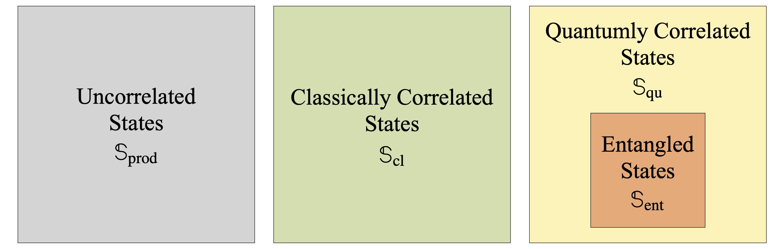
Figure 1: Schematic representation of different sets of states (not in scale). The totality of states is divided into three disjoint sets: uncorrelated (product) states in gray, classically correlated states in green, and quantumly correlated states in yellow. Entangled states are a subset of quantumly correlated states, and separable states are the ones that are not entangled.

The general entropic uncertainty principle between two non-degenerate observables $\mathit{X}$ and $\mathit{Y}$ that act on the same Hilbert space $\mathfrak{L}(\mathscr{H}_{d})$ is expressed by the following relation [12, 13]:

$$\mathbb{H}_{S}(\mathit{X})+\mathbb{H}_{S}(\mathit{Y})\geqslant-\log\Big(\max\limits_{i,j}|\innerproduct{x_{i}}{y_{j}}|^{2}\Big{missing}).$$ (1)

The term $-\log\big(\max_{i,j}|\innerproduct{x_{i}}{y_{j}}|^{2}\big{missing})\in[0,\log d]$ quantifies the incompatibility between the two observables, and the uncertainty principle asserts that the more certainty we have for the outcome of one observable the more uncertainty we have for the outcomes of the other, and vice versa (for other measures of incompatibility between the two observables see Refs. [14, 15]). Systems that contain only compatible observables are considered classical, while quantum systems can contain both compatible and incompatible observables. Two maximally incompatible observables are called complementary [16], denoted as $\mathit{X}\natural\mathit{Y}$, and have mutually unbiased bases (MUB), i.e.,

$$|\mbox{$\langle x_{i}|y_{j}\rangle$}|^{2}=\frac{1}{d}\quad\forall\,i,j\in\{0,\cdots,d-1\}.$$ (2)

The maximum number of pairwise complementary observables in $\mathfrak{L}(\mathscr{H}_{d})$ is equal to the maximum number of MUB in $\mathscr{H}_{d}$. For a Hilbert space $\mathscr{H}_{d}$, complete is called a set of MUB when it has $d+1$ elements. It is an open question whether a complete set of MUB exists for arbitrary dimensions [17], however it is known that the maximum number of MUB for any Hilbert space cannot exceed $d+1$, and that a complete set can always be found when $d$ is a power of a prime number  [18, 19, 20]. For example, when $d=2$ the Pauli matrices constitute a complete set of three pairwise complementary observables. For complementary observables in higher dimensions see Refs. [21, 22]. The significance of MUB can be seen by the fact that measurements on them provide enough information to fully reconstruct a state [23, 24, 25].

II.3 Correlations in Quantum Systems

Any bipartite state $S\in\mathfrak{L}(\mathscr{H}_{n})\otimes\mathfrak{L}(\mathscr{H}_{m})$ can be written in the Fano form [26, 27] as follows:

$$S=\frac{1}{d^{2}}\Bigg{(}\mathit{I}_{d}\otimes\mathit{I}_{d}+\sum_{i=1}^{d^{2}-1}n_{i}\mathit{\Lambda}_{i} \otimes\mathit{I}_{d}+\sum_{j=1}^{d^{2}-1}s_{j}\mathit{I}_{d}\otimes\mathit{\Lambda}_{j}$$

$$+\sum_{i,j=1}^{d^{2}-1}t_{ij}\mathit{\Lambda}_{i}\otimes\mathit{\Lambda}_{j}\Bigg{)},$$ (3)

where $d=\min\{n,m\}$ and $\{\mathit{\Lambda}_{i}\}_{i=1}^{d^{2}-1}$ is a Hermitian operator basis with $\mathrm{tr}(\mathit{\Lambda}_{i})=0$ and $\mathrm{tr}(\mathit{\Lambda}_{i}\mathit{\Lambda}_{j})=d\delta_{ij}$.

Quantifying correlations in quantum systems is a challenging task given that, unlike in classical systems, there are different types of correlations [28, 29]. More specifically, in regards to correlations there are two types of bipartite states: (i) uncorrelated states,

$$S_{\text{prod}}\coloneqq S^{(\text{A})}\otimes S^{(\text{B})},$$ (4)

also known as product states, and (ii) correlated states. Correlated states can be further classified as either: (i) classically correlated [30, 31, 32], that take the form:

$$S_{\text{cl}}\coloneqq\sum_{i,j}p_{ij}\outerproduct{e_{i}}{e_{i}}\otimes\outerproduct{h_{j}}{h_{j}},$$ (5)

where $\sum_{i,j}p_{ij}=1$, and $\{\ket{e_{i}}\}$, $\{\ket{h_{j}}\}$ being orthonormal bases, or (ii) quantumly correlated.

Remark 1.

A pure product state is considered classically correlated since it can be retrieved by taking the limit $p_{k\ell}\rightarrow 1$ in Eq. (5). This corresponds to the case where both parties have always the exact same state, and thus a pair of observables that contains perfectly correlated measurement outcomes can always be found.

Every classically correlated state can be written in the form of a separable state, i.e.,

$$S_{\text{sep}}\coloneqq\sum_{i}p_{i}S_{i}^{(\text{A})}\otimes S_{i}^{(\text{B})},$$ (6)

where $\sum_{i}p_{i}=1$, while the converse is not always true. Finally, quantumly correlated states that are not separable are called entangled [33] (see Refs. [34, 35] for a review of entanglement theory). In Fig. 1 we schematically represent all possible types of correlations in quantum systems. Note that the clear dichotomy between classically and quantumly correlated states is not a distinction that all authors accept. For example, as we discuss in the section II.3.1, an alternative view is that a state can be partially classically correlated and partially quantumly correlated.

Below, we introduce the two main ways correlations can be quantified in quantum systems.

II.3.1 Relative Entropy

One way—that we refer to as geometrical—to quantify the different types of correlations for a given bipartite state $S$ is by invoking a distant measure, e.g., relative entropy [4, 5] which for two states $S_{i}$ and $S_{j}$ is defined as

$$\mathbb{H}(S_{i}\|S_{j})\coloneqq\mathrm{tr}[S_{i}(\log_{2}S_{i}-\log_{2}S_{j})],$$ (7)

and minimize it over a certain class of states.

Based on this approach, quantum correlations, viz., discord, are measured as the minimum relative entropy of the state over all classically correlated states, $\mathrm{Q}(S)\coloneqq\min_{S_{\text{cl}}}\mathbb{H}(S\|S_{\text{cl}})$, [38], and entanglement as the minimum relative entropy of the state over all separable states, viz., relative entropy of entanglement, $\mathrm{E}(S)\coloneqq\min_{S_{\text{sep}}}\mathbb{H}(S\|S_{\text{sep}})$, [39]. The total correlations are measured as the minimum distance of the state over all uncorrelated states, which is equal to the mutual information $\mathbb{I}_{S}(\text{A}:\text{B})$, i.e. [38]

$$\mathrm{T}(S)\coloneqq\min_{S_{\text{prod}}}\mathbb{H}(S\|S_{\text{prod}})=\mathbb{H}(S\|S^{(\text{A})}\otimes S^{(\text{B})})\equiv\mathbb{I}_{S}(\text{A}:\text{B}).$$ (8)

Classical correlations are defined as $\mathrm{C}(S)\coloneqq\mathbb{H}(S\|\tilde{S}_{\text{prod}})-\mathbb{H}(S\|\tilde{S}_{\text{cl}})$, where $\tilde{S}_{\text{cl}}$ is the closest classical state to $S$, and $\tilde{S}_{\text{prod}}$ is the closest product state to $\tilde{S}_{\text{cl}}$.

Using this approach the total correlations of a state can be computed analytically, but this is not the case for classical correlations, quantum correlations, and entanglement (relative entropy of entanglement), for which in general no simple analytical expression is currently known. Note that this method implies that a quantum state can be partially correlated in a classical way and partially correlated in a quantum way, an idea that leads to the following issue.

Remark 2.

The total correlations measured through $\mathrm{T}(S)$ are not in general equal to the sum of the classical and quantum correlations: $\mathrm{C}(S)+\mathrm{Q}(S)$ [38]. An extra quantity to offset this imbalance can be introduced which however lacks a physical meaning.

II.3.2 Pearson Correlation Coefficient

A different way—that we refer to as statistical—to quantify the amount of correlations within a bipartite state is the Pearson correlation coefficient (PCC) [6]. Contrary to the geometrical method, which is calculated through the quantum states that comprise a quantum system, the PCC is directly calculated through pairs of observables that can be measured in a quantum system. In particular, for two observables that act on two different Hilbert spaces, $\mathit{A}\in\mathfrak{L}(\mathscr{H}_{d})$ and $\mathit{B}\in\mathfrak{L}(\mathscr{H}_{d})$, that have sample spaces of equal cardinality, the PCC is defined as

$$\mathbb{C}\mathrm{or}_{S}(\mathit{A},\mathit{B})\coloneqq\frac{\mathbb{C}\mathrm{ov}_{S}(\mathit{A},\mathit{B})}{\sqrt{\mathbb{V}_{S}(\mathit{A})\mathbb{V}_{S}(\mathit{B})}},$$ (9)

with $\mathbb{C}\mathrm{ov}_{S}(\mathit{A},\mathit{B})\coloneqq\mathbb{E}_{S}(\mathit{A}\otimes\mathit{B})-\mathbb{E}_{S}(\mathit{A})\mathbb{E}_{S}(\mathit{B})$ denoting the covariance between $\mathit{A}$ and $\mathit{B}$. $\mathbb{E}_{S}(\mathit{A})$, $\mathbb{E}_{S}(\mathit{B})$, and $\mathbb{E}_{S}(\mathit{A}\otimes\mathit{B})$ are the expectation values of $\mathit{A}$, $\mathit{B}$, and $\mathit{A}\otimes\mathit{B}$, respectively, and finally $\mathbb{V}_{S}(\mathit{A})$ and $\mathbb{V}_{S}(\mathit{B})$ the variances of $\mathit{A}$ and $\mathit{B}$, respectively. For an arbitrary observable $\mathit{X}$ the expectation value is defined as $\mathbb{E}_{S}(\mathit{X})\coloneqq\mathrm{tr}(S\mathit{X})$ and the variance as $\mathbb{V}_{S}(\mathit{X})\coloneqq\mathbb{E}_{S}(\mathit{X}^{2})-\mathbb{E}_{S}(\mathit{X})^{2}$. The range of the PCC lies within $[-1,1]$, where $+1$ implies perfect correlation and $-1$ perfect anti-correlation. For independent subsystems the PCC is zero for any pair of observables.

In both classical and quantum regimes the PCC quantifies only linear relationships between random variables and observables, respectively. General monotonic relationships are quantified by the Spearman rank correlation coefficient [40], which is defined classically as the PCC between random variables with ranked values, and in the quantum context we can immediately generalize it as the PCC between observables with ranked eigenspectra, i.e., eigenspectra that can be ranked in an ascending or a descending order. Note that for two dimensional observables the PCC coincides with the Spearman rank correlation coefficient.

III Total Correlations Through PCC

Figure 2: The bipartite states $S$ is measured in one Hilbert space by an observable $\mathit{A}_{i}$, with $k\in\{1,2,\cdots,v\}$ and in the other Hilbert space by an observable $\mathit{B}_{i}$, with $k\in\{1,2,\cdots,v\}$. Within each Hilbert space the observables are complementary, i.e., $\mathit{A}_{i}\natural\mathit{A}_{j}$ and $\mathit{B}_{i}\natural\mathit{B}_{j}$.

In this section we propose a method to quantify the total correlations in a quantum system based on the PCC. For an arbitrary bipartite state there are in general multiple pairs of observables that can be potentially correlated with each other. In order to capture all the available information in the state with the minimum amount of measurements, we consider the maximum set of complementary observables in the Hilbert space of each side as seen in Fig. 2. Also, in order to capture any possible type of correlations, i.e., not only linear, we consider observables with ordered eigenspectra. Thus, for the ordered observables $\{(\mathit{A}_{i},\mathit{B}_{i})\}_{i=1}^{v}$, where $v$ is the cardinality of the maximum set of pairwise complementary observables in the Hilbert space $\mathfrak{L}(\mathscr{H}_{d})$, the sum of the correlations of a bipartite state $S$ is

$$\sum_{i=1}^{v}|\mathbb{C}\mathrm{or}_{S}(\mathit{A}_{i},\mathit{B}_{i})|.$$ (10)

In Ref. [41] it was shown that for a specific set of observables and for certain families of states a sum of the PCC values is connected to the entanglement measure Negativity [42, 43, 44].

Even though it is reasonable for correlations to depend on the measured observables, in quantum information theory, expressions that quantify correlations are typically defined in such a way so they are invariant under local unitary transformations. Thus, we define the measure for total correlations as follows

$$\mathbb{R}_{S}(\text{A}:\text{B})\coloneqq\max_{\{\mathit{A}_{i},\mathit{B}_{i}\}}\sum_{i=1}^{v}|\mathbb{C}\mathrm{or}_{S}(\mathit{A}_{i},\mathit{B}_{i})|,$$ (11)

where the maximization is taken over all possible pairs of complementary observables.

Remark 3.

When the maximum number of complementary observables is not known, $v$ is substituted by the maximum known cardinality of the set of complementary observables, and the above expression becomes a lower bound of the total correlations.

It can be easily seen that for any bipartite state the total correlations are at least as large as the maximum correlations of a single pair of observables, i.e., $\mathbb{R}_{S}(\text{A}:\text{B})\geqslant\max_{\{\mathit{A},\mathit{B}\}}|\mathbb{C}\mathrm{or}_{S}(\mathit{A},\mathit{B})|$. In the section below we focus on two-dimensional bipartite states, that we refer to as two-qubit states, and show what is the implication when this inequality becomes an equality.

IV Total correlations in two-Qubit States

Let us focus in this section on two-qubit states and two-dimensional observables. Given that the absolute PCC value is invariant under affine transformations, without loss of generality we can always consider observables that have dichotomic outcomes: $\pm 1$. Complementary observables with such eigenvalues are always orthogonal to each other [7], so any triplet of them constitutes a Hermitian operator basis.

Theorem 1.

A necessary condition for a two-qubit state to be classically correlated is the ability of its total correlations to be concentrated using local unitary operations in a single pair of observables, i.e.,

$$\mathbb{R}_{S}(\text{A}:\text{B})=\max_{\{\mathit{A},\mathit{B}\}}|\mathbb{C}\mathrm{or}_{S}(\mathit{A},\mathit{B})|.$$ (12)

Proof.

Every classically correlated two-qubit state [see Eq. (5)] can be diagonalized through local unitary operations (which leave the total correlations invariant), so it can take the following form:

$$S_{\text{cl}}=\frac{1}{4}\big{(}\mathit{I}_{2}\otimes\mathit{I}_{2}+n_{3}\mathit{\Lambda}_{3}\otimes\mathit{I}_{2}+s_{3}\mathit{I}_{2}\otimes\mathit{\Lambda}_{3}+t_{33}\mathit{\Lambda}_{3}\otimes\mathit{\Lambda}_{3}\big{)},$$ (13)

where $\mathit{\Lambda}_{3}=\begin{bmatrix}1&0\\ 0&-1\end{bmatrix}$.

The PCC for two arbitrary observables $(\mathit{A},\mathit{B})$ is equal to

$$\mathbb{C}\mathrm{or}_{S_{\text{cl}}}(\mathit{A},\mathit{B})=\frac{\frac{t_{33}-n_{3}s_{3}}{4}\mathrm{tr}(\mathit{A}\mathit{\Lambda}_{3})\mathrm{tr}(\mathit{B}\mathit{\Lambda}_{3})}{\sqrt{\left[1-\frac{n_{i}^{2}}{4}\mathrm{tr}(\mathit{A}\mathit{\Lambda}_{3})^{2}\right]\left[1-\frac{s_{i}^{2}}{4}\mathrm{tr}(\mathit{B}\mathit{\Lambda}_{3})^{2}\right]}},$$ (14)

since $\mathbb{E}_{S_{\text{cl}}}(\mathit{A}\otimes\mathit{I}_{2})=\frac{1}{2}n_{3}\mathrm{tr}\left(\mathit{A}\mathit{\Lambda}_{3}\right)$, $\mathbb{E}_{S_{\text{cl}}}(\mathit{I}_{2}\otimes\mathit{B})=\frac{1}{2}s_{3}\mathrm{tr}\left(\mathit{B}\mathit{\Lambda}_{3}\right)$, and $\mathbb{E}_{S_{\text{cl}}}(\mathit{A}\otimes\mathit{B})=\frac{1}{4}t_{33}\mathrm{tr}\left(\mathit{A}\mathit{\Lambda}_{3}\right)\mathrm{tr}\left(\mathit{B}\mathit{\Lambda}_{3}\right)$. Given that $\mathrm{tr}(\mathit{A}\mathit{\Lambda}_{3})\in[-2,2]$ and $\mathrm{tr}(\mathit{B}\mathit{\Lambda}_{3})\in[-2,2]$, we have

$$\max_{\{\mathit{A},\mathit{B}\}}|\mathbb{C}\mathrm{or}_{S_{\text{cl}}}(\mathit{A},\mathit{B})|=\frac{|t_{33}-n_{3}s_{3}|}{\sqrt{\left(1-n_{3}^{2}\right)\left(1-s_{3}^{2}\right)}},$$ (15)

that is reachable when $\mathit{A}=\mathit{\Lambda}_{3}$ and $\mathit{B}=\mathit{\Lambda}_{3}$.

For the sum of correlations we have

$$\sum_{i=1}^{3}\frac{|t_{33}{-}n_{3}s_{3}||\mathrm{tr}(\mathit{A}_{i}\mathit{\Lambda}_{3})\mathrm{tr}(\mathit{B}_{i}\mathit{\Lambda}_{3})|}{4\sqrt{\left[1{-}\frac{n_{3}^{2}}{4}\mathrm{tr}(\mathit{A}_{i}\mathit{\Lambda}_{3})^{2}\right]\left[1{-}\frac{s_{3}^{2}}{4}\mathrm{tr}(\mathit{B}_{i}\mathit{\Lambda}_{3})^{2}\right]}}$$ (16a)

$$\leqslant\frac{|t_{33}-n_{3}s_{3}|}{4\sqrt{(1-n_{3}^{2})(1-s_{3}^{2})}}\sum_{i=1}^{3}|\mathrm{tr}(\mathit{A}_{i}\mathit{\Lambda}_{3})\mathrm{tr}(\mathit{B}_{i}\mathit{\Lambda}_{3})|.$$ (16b)

Using the Cauchy-Schwarz inequality, we obtain

$$\sum_{i=1}^{3}|\mathrm{tr}(\mathit{A}_{i}\mathit{\Lambda}_{3})\mathrm{tr}(\mathit{B}_{i}\mathit{\Lambda}_{3})|\leqslant\sqrt{\sum_{i=1}^{3}\mathrm{tr}(\mathit{A}_{i}\mathit{\Lambda}_{3})^{2}\sum_{i=1}^{3}\mathrm{tr}(\mathit{B}_{i}\mathit{\Lambda}_{3})^{2}},$$ (17)

which, due to the Parseval’s identity, is simplified to

$$\sum_{i=1}^{3}|\mathrm{tr}(\mathit{A}_{i}\mathit{\Lambda}_{3})\mathrm{tr}(\mathit{B}_{i}\mathit{\Lambda}_{3})|\leqslant 4.$$ (18)

Thus, the maximum sum of correlations is equal to

$$\mathbb{R}_{S_{\text{cl}}}(\text{A}:\text{B})=\frac{|t_{33}-n_{3}s_{3}|}{\sqrt{(1-n_{3}^{2})(1-s_{3}^{2})}},$$ (19)

that is reachable when $\mathit{A}_{i}=\mathit{B}_{i}=\mathit{\Lambda}_{i}$ for every $i\in\{1,2,3\}$, which completes the proof. ∎

The above result implies the following sufficient condition for a two-qubit state to be quantumly correlated.

Corollary 1.

A sufficient condition for a two-qubit state to be quantumly correlated is its total correlations to be over one.

Proof.

Based on Theorem 1 any classically correlated two-qubit state can concentrate its total correlations into a single pair of observables. However, the correlations of every single pair cannot exceed one. Thus, it is easy to see that if the total correlations of a state exceed one then the state must be quantumly correlated. ∎

Figure 3: In panel (a) the total correlations of Werner states $S_{\text{W}}$ and Horodecki states $S_{\text{H}}$ [see Eqs. (27) and (28)] are quantified by the PCC-based measure $\mathbb{R}_{S}(\text{A}:\text{B})$ and the mutual information $\mathbb{I}_{S}(\text{A}:\text{B})$. In panels (b)-(f) specific points are isolated and analyzed in terms of the PCC of each observable pair. It is clear that the PCC provides in general more granularity indicating how the correlations are distributed among the pairs of observables in the system, but more importantly it can detect classical correlations which are not identified by the mutual information as seen in panel (c).

Let us consider now two-qubit states written in the special form

$$S_{\text{sf}}=\frac{1}{4}\bigg{(}\mathit{I}_{2}\otimes\mathit{I}_{2}+n_{k}\mathit{\Lambda}_{k}\otimes\mathit{I}_{2}+s_{k}\mathit{I}_{2}\otimes\mathit{\Lambda}_{k}+\sum_{i=1}^{3}\lambda_{i}\mathit{\Lambda}_{i}\otimes\mathit{\Lambda}_{i}\bigg{)},$$ (20)

where $\{\mathit{\Lambda_{k}}\}_{k=1}^{3}$ are the Pauli matrices. When $n_{k}=s_{k}=0$ the states are in the so-called standard form [45]. Those are the states that become maximally mixed when one of the two parts is traced out, and are also known as Bell-diagonal states, since they can be written as a mixture of the four Bell states. A two-qubit state in the standard form is classically correlated if and only if it has only one non-zero coefficient $\lambda_{k}$ [36]. The more general state in Eq. (20) becomes classically correlated when there is only one non-zero coefficient $\lambda_{i}$ and the coefficients $n_{k}$ and $s_{k}$ have the same index value as the non-zero $\lambda$ coefficient, e.g., see Eq. (13).

Theorem 2.

A necessary and sufficient condition for a two-qubit state in the special form to be classically correlated is the ability of its total correlations to be concentrated using local unitary operations in a pair of observables, i.e.,

$$\mathbb{R}_{S_{\text{sf}}}(\text{A}:\text{B})=\max_{\{\mathit{A},\mathit{B}\}}|\mathbb{C}\mathrm{or}_{S_{\text{sf}}}(\mathit{A},\mathit{B})|.$$ (21)

Proof.

The necessity of this condition directly follows from Theorem 1, so we only need to prove the sufficiency of it. Consider two observables decomposed as follows: $\mathit{A}=a_{0}\mathit{I}_{2}+\sum_{k=1}^{3}a_{k}\,\mathit{\Lambda}_{k}$ and $\mathit{B}=b_{0}\mathit{I}_{2}+\sum_{k=1}^{3}b_{k}\,\mathit{\Lambda}_{k}$. Then, we can represent each observable as a normalized column vector $\ket{a}=[a_{1},a_{2},a_{3}]$ and $\ket{b}=[b_{1},b_{2},b_{3}]$. For two-qubit states the PCC can be re-written as [7]

$$\mathbb{C}\mathrm{or}_{S}(\mathit{A},\mathit{B})=\frac{\bra{a}\mathit{C}\ket{b}}{\sqrt{1-\innerproduct{a}{n}^{2}}\sqrt{1-\innerproduct{b}{s}^{2}}},$$ (22)

where $\mathit{C}$ is a matrix with elements $c_{ij}=\sum_{i,j=1}^{3}t_{ij}-n_{i}s_{j}$ [see Eq. (II.3)], and $\ket{n}$ and $\ket{s}$ the column vectors $[n_{1},n_{2},n_{3}]$ and $[s_{1},s_{2},s_{3}]$, respectively. Then, we have

$$\mathbb{C}\mathrm{or}_{S}(\mathit{A},\mathit{B})\leqslant\frac{\bra{a}\mathit{C}\ket{b}}{\sqrt{1-\innerproduct{n}{n}^{2}}\sqrt{1-\innerproduct{s}{s}^{2}}},$$ (23)

since $\innerproduct{a}{n}^{2}\leqslant\sum_{i=1}^{3}\innerproduct{a_{i}}{n}^{2}=\sum_{i=1}^{3}n_{i}^{2}=\innerproduct{n}{n}$, and analogously $\mbox{$\langle b|s\rangle$}^{2}\leqslant\innerproduct{s}{s}$. Recalling that the spectral norm is defined as ${\left|\kern-1.07639pt\left|\kern-1.07639pt\left|\mathit{C}\right|\kern-1.07639pt\right|\kern-1.07639pt\right|}_{2}=\max_{\bigl{\{}\mbox{$\langle a|$},\mbox{$|b\rangle$}\bigl{\}}}|\bra{a}\mathit{C}\ket{b}|$ [46], we obtain

$$\max_{\{\mathit{A},\mathit{B}\}}|\mathbb{C}\mathrm{or}_{S}(\mathit{A},\mathit{B})|=\frac{{\left|\kern-1.07639pt\left|\kern-1.07639pt\left|\mathit{C}\right|\kern-1.07639pt\right|\kern-1.07639pt\right|}_{2}}{\sqrt{1-\innerproduct{n}{n}^{2}}\sqrt{1-\innerproduct{s}{s}^{2}}},$$ (24)

where ${\left|\kern-1.07639pt\left|\kern-1.07639pt\left|\mathit{C}\right|\kern-1.07639pt\right|\kern-1.07639pt\right|}_{2}$ is equal to the maximum singular value of $\mathit{C}$. It was also shown in Ref. [7], that for two-qubit states we have

$$\mathbb{R}_{S}(\mathit{A}_{i}:\mathit{B}_{i})=\frac{{\left|\kern-1.07639pt\left|\kern-1.07639pt\left|\mathit{C}\right|\kern-1.07639pt\right|\kern-1.07639pt\right|}_{\text{tr}}}{\sqrt{1-\innerproduct{n}{n}^{2}}\sqrt{1-\innerproduct{s}{s}^{2}}},$$ (25)

where ${\left|\kern-1.07639pt\left|\kern-1.07639pt\left|\mathit{C}\right|\kern-1.07639pt\right|\kern-1.07639pt\right|}_{\text{tr}}$ denotes the trace norm of $\mathit{C}$, i.e., the sum of its singular values [46].

Thus, for two-qubit states in the special form the condition $\mathbb{R}_{S_{\text{sf}}}(\mathit{A}_{i}:\mathit{B}_{i})=\max_{\{\mathit{A},\mathit{B}\}}|\mathbb{C}\mathrm{or}_{S_{\text{sf}}}(\mathit{A},\mathit{B})|$ is equivalent to the condition ${\left|\kern-1.07639pt\left|\kern-1.07639pt\left|\mathit{C}\right|\kern-1.07639pt\right|\kern-1.07639pt\right|}_{\text{tr}}={\left|\kern-1.07639pt\left|\kern-1.07639pt\left|\mathit{C}\right|\kern-1.07639pt\right|\kern-1.07639pt\right|}_{2}$, i.e.,

$$\sum_{i=1}^{3}|\lambda_{i}-n_{i}s_{i}|=\max\{\lambda_{1}-n_{1}s_{1},\lambda_{2}-n_{2}s_{2},\lambda_{3}-n_{3}s_{3}\},$$ (26)

that is true only when the state is classically correlated, which completes the proof. ∎

Remark 4.

Eq. (26) shows that the maximum correlations (individual and total) in two-qubit states in the special form are achieved when the measurements are made in the Hermitian operator basis that the state is decomposed in Eq. (20).

V Discussion

In Fig. 3 we compare the two ways total correlations can be quantified: through the expression $\mathbb{R}_{S}(\text{A}:\text{B})$ and through mutual information $\mathbb{I}_{S}(\text{A}:\text{B})$. We pick two states for this comparison: the state

$$S_{\text{W}}\coloneqq p\mathit{\Phi}+(1-p)\mathit{I}_{4},$$ (27)

namely the Werner state, where $\mathit{\Phi}=\outerproduct{\phi}{\phi}$ is the Bell state with $\ket{\phi}=(\ket{00}+\ket{11})/\sqrt{2}$, and the state

$$S_{\text{H}}\coloneqq p\mathit{\Phi}+(1-p)\mathit{\Pi}_{0},$$ (28)

which is a variation of the so-called Horodecki state, where $\mathit{\Pi}_{0}=\outerproduct{00}{00}$. In panel (a) we plot the total correlations for both states through both methods. Note that the three optimal pairs of observables in Eq. (11) for both states are: $(\mathit{\Lambda_{1},\mathit{\Lambda}_{1}})$, $(\mathit{\Lambda_{2},\mathit{\Lambda}_{2}})$, and $(\mathit{\Lambda_{3},\mathit{\Lambda}_{3}})$, due to Remark 4. When $p=1$ both states are in the Bell state $\mathit{\Phi}$, so both expressions reach their maximum value. In panel (f) we focus on the value $p=1$, for which the PCC of all three pairs reaches unity. For $1/3<p\leqslant 1$, $S_{\text{W}}$ is entangled, and focusing in particular in the case for $p=1/3$ we see in panel (d) that the PCC’s of all three pairs are equal to 1/3, summing up to 1, which is the separability threshold. On the other hand, the corresponding value $\mathbb{I}_{S_{\text{W}}}(\text{A}:\text{B})\simeq 0.21$ for $p=1/3$ does not constitute a separability bound. $S_{\text{H}}$ is entangled for any $p>0$, which is also reflected in panel (a) since $\mathbb{R}_{S_{\text{H}}}(\text{A}:\text{B})$ is always above the unity threshold. In panel (e) we see that $S_{\text{H}}$ for $p=1/3$ has perfect correlations for one of the three observable pairs while for the other two the correlations are equal to 1/3. In that case $\mathbb{I}_{S_{\text{H}}}(\text{A}:\text{B})\simeq 0.75$. When $p=0$, $S_{\text{W}}$ becomes the maximally mixed state, and both $\mathbb{R}_{S_{\text{W}}}(\text{A}:\text{B})$ and $\mathbb{I}_{S_{\text{W}}}(\text{A}:\text{B})$ become equal to zero. In panel (b) we see how all PCC’s vanish for $p=0$ for $S_{\text{W}}$. Interestingly, the two expressions provide different perspectives for $S_{\text{H}}$ with $p=0$, since $\mathbb{R}_{S_{\text{H}}}(\text{A}:\text{B})=1$ and $\mathbb{I}_{S_{\text{H}}}(\text{A}:\text{B})=0$. In that case $S_{\text{H}}=\mathit{\Pi}_{0}$ is a classically correlated state (see Remark 1), and as seen in panel (c) the PCC-based expression captures that fact, where the PCC of one of the three pairs is equal to one, which is the maximum value for classical correlations, while the other two are zero. Examples like this, provide evidence that the expression $\mathbb{R}_{S}(\text{A}:\text{B})$ is more appropriate for the quantification of total correlations than $\mathbb{I}_{S}(\text{A}:\text{B})$.

As we discussed in Remark 2, assessing correlations through distance-based measures leads to an issue, which can be avoided all together if we abandon the assumption that quantum states can simultaneously be classically and quantumly correlated. Using our method, the notion of correlation remains the same regardless of the system [given by Eq. (9)], and then the distinction between classical and quantum correlated states depends on whether multiple pairs of observables are simultaneously correlated (recall that the pairs of observables are not arbitrary but within each partition the considered observables are mutually incompatible as seen in Fig. 2). For example the states in panels (c) and (d) have the same total correlations, however, the state in panel (c) is a classically correlated state because only one pair of observables is correlated, but the state in panel (d) is a quantumly correlated state since all three pairs are correlated.

More broadly, our analysis suggests that different types of correlations appear as different distributions of the PCC values between pairs of observables. For the special case of two-qubit states in the special form, we were able to show that the maximum total correlations can be concentrated in a single pair of observables if and only if the state is classically correlated. Numerical analysis provides us evidence that the same condition should hold for any two-qubit quantum state, even though a rigorous proof is currently missing. For higher-dimensional states it is yet unclear how exactly the distribution of the PCC values is related to the nature of the correlations in the system, and more work is needed in this direction.

It is now clear how classical and quantum correlations are connected to the uncertainty principle, i.e., complementarity, and why entanglement is commonly referred to as a “stronger type of correlation” in comparison to the classical ones. Perfect correlations between two observables can exist in both classical and quantum systems. However, the fundamental difference between the two types of correlations is that in quantum systems multiple pairs of observables can be simultaneously correlated (even perfectly) while being locally incompatible (see Fig. 2), a phenomenon that is impossible in classical systems, where observables are necessarily locally compatible.

VI Conclusions

In this work, we introduced a framework for the quantification of total correlations in quantum systems through the Pearson correlation coefficient. For two-qubit states in particular, we showed how quantum correlations are connected to the uncertainty principle, and how classically and quantumly correlated states can be distinguished based on the correlations between two specific sets of observables. These sets correspond to two locally complementary observables, which are also useful for other tasks, such as quantum state estimation [23, 24, 25], entanglement detection [47, 6], quantum cryptography [48, 49], quantum retrodiction [50, 51]. An interesting future path of this work would be to show that the condition in Theorem 1 is not only necessary but also sufficient, and potentially extend this result to higher-dimensional and/or multi-partite quantum states.

VII Acknowledgements

This work is supported by the National Science Foundation under grant number NSF CNS 2106887 on “U.S.-Ireland R&D Partnership: Collaborative Research: CNS Core: Medium: A unified framework for the emulation of classical and quantum physical layer networks”, the NSF QuIC-TAQS program “QuIC-TAQS: Deterministically Placed Nuclear Spin Quantum Memories for Entanglement Distribution” under grant number NSF OMA 2137828, the NSF CAREER: First Principles Design of Error-Corrected Solid-State Quantum Repeaters under grant number #1944085, the Australian Research Council Centre of Excellence CE170100012, Laureate Fellowship FL150100019, and the Australian Government Research Training Program Scholarship.

References

- Pearson and Galton [1895] K. Pearson and F. Galton, VII. Note on regression and inheritance in the case of two parents, Proc. R. Soc. Lond. 58, 347 (1895).
- Rényi [2007] A. Rényi, Probability Theory, 1st ed. (Dover Publications, Mineola, NY, 2007).
- Cover and Thomas [2006] T. M. Cover and J. A. Thomas, Elements of Information Theory, 2nd ed. (John Wiley & Sons, Inc., Hoboken, NJ 07030, 2006).
- Umegaki [1962] H. Umegaki, Conditional expectation in an operator algebra. iv. entropy and information, Kodai Math. J. 14 (1962).
- Vedral [2002] V. Vedral, The role of relative entropy in quantum information theory, Rev. Mod. Phys. 74, 197 (2002).
- Maccone et al. [2015] L. Maccone, D. Bruß, and C. Macchiavello, Complementarity and correlations, Phys. Rev. Lett. 114, 130401 (2015).
- [7] S. Tserkis et al. (manuscript under review) .
- Pozsgay et al. [2017] V. Pozsgay, F. Hirsch, C. Branciard, and N. Brunner, Covariance Bell inequalities, Phys. Rev. A 96, 062128 (2017).
- Huang and Vontobel [2021] Y. Huang and P. O. Vontobel, Sets of marginals and pearson-correlation-based chsh inequalities for a two-qubit system, in 2021 IEEE International Symposium on Information Theory (ISIT) (IEEE, 2021) pp. 1338–1343.
- Kothe and Björk [2007] C. Kothe and G. Björk, Entanglement quantification through local observable correlations, Phys. Rev. A 75, 012336 (2007).
- Abascal and Björk [2007] I. S. Abascal and G. Björk, Bipartite entanglement measure based on covariance, Phys. Rev. A 75, 062317 (2007).
- Kraus [1987] K. Kraus, Complementary observables and uncertainty relations, Phys. Rev. D 35, 3070 (1987).
- Maassen and Uffink [1988] H. Maassen and J. B. M. Uffink, Generalized entropic uncertainty relations, Phys. Rev. Lett. 60, 1103 (1988).
- Heinosaari et al. [2016] T. Heinosaari, T. Miyadera, and M. Ziman, An invitation to quantum incompatibility, J. Phys. A Math. Theor. 49, 123001 (2016).
- Gühne et al. [2023] O. Gühne, E. Haapasalo, T. Kraft, J.-P. Pellonpää, and R. Uola, Colloquium: Incompatible measurements in quantum information science, Rev. Mod. Phys. 95, 011003 (2023).
- Schwinger [1960] J. Schwinger, Unitary operator bases, Proc. Nat. Acad. Sci. 46, 570 (1960).
- Horodecki et al. [2022] P. Horodecki, L. Rudnicki, and K. Życzkowski, Five open problems in quantum information theory, PRX Quantum 3, 010101 (2022).
- Ivonovic [1981] I. D. Ivonovic, Geometrical description of quantal state determination, J. Phys. A Math. Gen. 14, 3241 (1981).
- Wootters and Fields [1989] W. K. Wootters and B. D. Fields, Optimal state-determination by mutually unbiased measurements, Ann. Phys. 191, 363 (1989).
- Bandyopadhyay et al. [2002] S. Bandyopadhyay, P. O. Boykin, V. Roychowdhury, and F. Vatan, A new proof for the existence of mutually unbiased bases, Algorithmica 34, 512 (2002).
- Lawrence [2004] J. Lawrence, Mutually unbiased bases and trinary operator sets for qutrits, Phys. Rev. A 70, 012302 (2004).
- Brierley et al. [2010] S. Brierley, S. Weigert, and I. Bengtsson, All mutually unbiased bases in dimensions two to five, Quantum Info. Comput. 10, 803–820 (2010).
- Adamson and Steinberg [2010] R. B. A. Adamson and A. M. Steinberg, Improving quantum state estimation with mutually unbiased bases, Phys. Rev. Lett. 105, 030406 (2010).
- Fernández-Pérez et al. [2011] A. Fernández-Pérez, A. B. Klimov, and C. Saavedra, Quantum process reconstruction based on mutually unbiased basis, Phys. Rev. A 83, 052332 (2011).
- Petz and Ruppert [2012] D. Petz and L. Ruppert, Efficient quantum tomography needs complementary and symmetric measurements, Rep. Math. Phys. 69, 161 (2012).
- Fano [1983] U. Fano, Pairs of two-level systems, Rev. Mod. Phys. 55, 855 (1983).
- Schlienz and Mahler [1995] J. Schlienz and G. Mahler, Description of entanglement, Phys. Rev. A 52, 4396 (1995).
- Adesso et al. [2016] G. Adesso, T. R. Bromley, and M. Cianciaruso, Measures and applications of quantum correlations, J. Phys. A Math. Theor. 49, 473001 (2016).
- Modi et al. [2012] K. Modi, A. Brodutch, H. Cable, T. Paterek, and V. Vedral, The classical-quantum boundary for correlations: Discord and related measures, Rev. Mod. Phys. 84, 1655 (2012).
- Henderson and Vedral [2001] L. Henderson and V. Vedral, Classical, quantum and total correlations, J. of Phys. A: Math. Gen. 34, 6899 (2001).
- Ollivier and Zurek [2001] H. Ollivier and W. H. Zurek, Quantum discord: A measure of the quantumness of correlations, Phys. Rev. Lett. 88, 017901 (2001).
- Oppenheim et al. [2002] J. Oppenheim, M. Horodecki, P. Horodecki, and R. Horodecki, Thermodynamical approach to quantifying quantum correlations, Phys. Rev. Lett. 89, 180402 (2002).
- Werner [1989] R. F. Werner, Quantum states with einstein-podolsky-rosen correlations admitting a hidden-variable model, Phys. Rev. A 40, 4277 (1989).
- Horodecki et al. [2009] R. Horodecki, P. Horodecki, M. Horodecki, and K. Horodecki, Quantum entanglement, Rev. Mod. Phys. 81, 865 (2009).
- Plenio and Virmani [2014] M. B. Plenio and S. S. Virmani, An introduction to entanglement theory, in Quantum Information and Coherence, edited by E. Andersson (Springer International Publishing, Cham, 2014) pp. 173–209.
- Dakić et al. [2010] B. Dakić, V. Vedral, and C. Brukner, Necessary and sufficient condition for nonzero quantum discord, Phys. Rev. Lett. 105, 190502 (2010).
- Bellomo et al. [2012] B. Bellomo, G. L. Giorgi, F. Galve, R. Lo Franco, G. Compagno, and R. Zambrini, Unified view of correlations using the square-norm distance, Phys. Rev. A 85, 032104 (2012).
- Modi et al. [2010] K. Modi, T. Paterek, W. Son, V. Vedral, and M. Williamson, Unified view of quantum and classical correlations, Phys. Rev. Lett. 104, 080501 (2010).
- Vedral et al. [1997] V. Vedral, M. B. Plenio, M. A. Rippin, and P. L. Knight, Quantifying entanglement, Phys. Rev. Lett. 78, 2275 (1997).
- Spearman [1906] C. Spearman, ‘Footrule’ for measuring correlation, Br. J. Psychol. 2, 89 (1906).
- Simanraj Sadana [2022] D. H. U. S. Simanraj Sadana, Som Kanjilal, Relating an entanglement measure with statistical correlators for two-qudit mixed states using only a pair of complementary observables, Preprint at arXiv:2201.06188 (2022).
- Życzkowski et al. [1998] K. Życzkowski, P. Horodecki, A. Sanpera, and M. Lewenstein, Volume of the set of separable states, Phys. Rev. A 58, 883 (1998).
- Lee et al. [2000] J. Lee, M. S. Kim, Y. J. Park, and S. Lee, Partial teleportation of entanglement in a noisy environment, J. Mod. Opt. 47, 2151 (2000).
- Vidal and Werner [2002] G. Vidal and R. F. Werner, Computable measure of entanglement, Phys. Rev. A 65, 032314 (2002).
- Leinaas et al. [2006] J. M. Leinaas, J. Myrheim, and E. Ovrum, Geometrical aspects of entanglement, Phys. Rev. A 74, 012313 (2006).
- Horn and Johnson [2013] R. A. Horn and C. R. Johnson, Matrix Analysis, 2nd ed. (Cambridge University Press, New York, NY, 2013).
- Spengler et al. [2012] C. Spengler, M. Huber, S. Brierley, T. Adaktylos, and B. C. Hiesmayr, Entanglement detection via mutually unbiased bases, Phys. Rev. A 86, 022311 (2012).
- Bennett and Brassard [1984] C. H. Bennett and G. Brassard, Quantum cryptography: Public key distribution and coin tossing, Proceedings of the IEEE International Conference on Computers, Systems and Signal Processing, Bangalore , 175 (1984).
- Cerf et al. [2002] N. J. Cerf, M. Bourennane, A. Karlsson, and N. Gisin, Security of quantum key distribution using -level systems, Phys. Rev. Lett. 88, 127902 (2002).
- Englert and Aharonov [2001] B.-G. Englert and Y. Aharonov, The mean king’s problem: prime degrees of freedom, Phys. Lett. A 284, 1 (2001).
- Reimpell and Werner [2007] M. Reimpell and R. F. Werner, Meaner king uses biased bases, Phys. Rev. A 75, 062334 (2007).