Computational Asymmetries in Robust Classification

Abstract

In the context of adversarial robustness, we make three strongly related contributions. First, we prove that while attacking ReLU classifiers is $\mathit{NP}$-hard, ensuring their robustness at training time is $\Sigma^{2}_{P}$-hard (even on a single example). This asymmetry provides a rationale for the fact that robust classifications approaches are frequently fooled in the literature. Second, we show that inference-time robustness certificates are not affected by this asymmetry, by introducing a proof-of-concept approach named Counter-Attack (CA). Indeed, CA displays a reversed asymmetry: running the defense is $\mathit{NP}$-hard, while attacking it is $\Sigma_{2}^{P}$-hard. Finally, motivated by our previous result, we argue that adversarial attacks can be used in the context of robustness certification, and provide an empirical evaluation of their effectiveness. As a byproduct of this process, we also release UG100, a benchmark dataset for adversarial attacks.

1 Introduction

Adversarial attacks, i.e. algorithms designed to fool machine learning models, represent a significant threat to the applicability of such models in real-world contexts (Brown et al., 2017; Brendel et al., 2019; Wu et al., 2020). Despite years of research effort, countermeasures (i.e. “defenses”) to adversarial attacks are frequently fooled by applying small tweaks to existing techniques (Carlini & Wagner, 2016, 2017a; He et al., 2017; Hosseini et al., 2019; Tramer et al., 2020; Croce et al., 2022). We argue that this pattern is due to differences between the fundamental mathematical problems that defenses and attacks need to tackle, and we investigate this topic by providing three contributions.

First, we prove a set of theoretical results about the complexity of attack and training-time defense problems, including the fact that attacking a ReLU classifier is $\mathit{NP}$-hard in the general case, while finding a parameter set that makes a ReLU classifier robust on even a single input is $\Sigma_{2}^{P}$-hard. To the best of our knowledge, this is the first complexity bound for general ReLU classifiers, and the main contribution of this work. We also provide more general bounds for non-polynomial classifiers, and show in particular that an $A$-time classifier can be attacked in $\mathit{NP}^{A}$ time. Instead of using a PAC-like formalization, we rely on a worst-case semantic of robustness. This approach results in a formalization that is both more easier to deal with and independent of data distribution assumptions, while still providing a rationale for difficulties in training robust classifiers that are well-known in the related literature. Our proofs also lay the ground work for identifying tractable classes of defenses.

Second, we prove by means of an example that inference-time defenses can sidestep the asymmetry. Our witness is a proof-of-concept approach, referred to as Counter-Attack (CA), that evaluates robustness on the fly for a specific input (w.r.t. to a maximum distance $\varepsilon$) by running an adversarial attack. Properties enjoyed by this technique are likely to extend to other inference-time defense methods, if they are based on similar principles. Notably, when built over an exact attack, generating a certificate is $\mathit{NP}$-hard in the worst case, $\varepsilon$-bounded attacks are impossible, and attacking using perturbations of magnitude $\varepsilon^{\prime}>\varepsilon$ is $\Sigma_{2}^{P}$-hard. On the other hand, using a non-exact attack results in partial guarantees (no false positives for heuristic attacks, no false negatives for bounding techniques).

Finally, since our results emphasize the connection between verification and attack problems, we provide an empirical investigation of the use of heuristic attacks for verification. We found heuristic attacks to be high-quality approximators for exact decision boundary distances: a pool of seven heuristic attacks provided an accurate (average over-estimate between 2.04% and 4.65%) and predictable (average $R^{2}>0.99$) approximation of the true optimum for small-scale Neural Networks trained on the MNIST and CIFAR10 datasets. We release our benchmarks and adversarial examples (both exact and heuristic) in a new dataset, named UG100.

Overall, we hope our contributions can support future research by highlighting potential structural challenges, pointing out key sources of complexity, inspiring research on heuristics and tractable classes, and suggesting alternative perspectives on how to build robust classifiers.

2 Background and Formalization

In this section, we introduce key definitions (adapted from Dreossi et al. (2019)) that we will use to frame our results. Our aim is to capture the key traits shared by most of the literature on adversarial attacks, so as to identify properties that are valid under broad assumptions.

Adversarial Attacks and Robustness

We start by defining the concept of adversarial example, which intuitively represents a modification of a legitimate input that is so limited as to be inconsequential for a human observer, but sufficient to mislead a target model. Formally, let $f:X\to\{1,\dots,N\}$ be a discrete classifier. Let $B_{p}({\bm{x}},\varepsilon)=\{{\bm{x}}^{\prime}\in X\,|\,\|{\bm{x}}-{\bm{x}}^{\prime}\|_{p}\leq\varepsilon\}$ be a $L^{p}$ ball of radius $\varepsilon$ and center ${\bm{x}}$. Then we have:

Definition 2.1 (Adversarial Example).

Given an input ${\bm{x}}$, a threshold $\varepsilon$, and a $L^{p}$ norm, an adversarial example is an input ${\bm{x}}^{\prime}\in B_{p}({\bm{x}},\varepsilon)$ such that $f({\bm{x}}^{\prime})\in C({\bm{x}})$, where $C({\bm{x}})\subseteq\{1,\dots,N\}\setminus\{f({\bm{x}})\}$.

This definition is a simplification compared to human perception, but it is adequate for a sufficiently small $\varepsilon$, and it is adopted in most of the relevant literature. An adversarial attack can then be viewed as an optimization procedure that attempts to find an adversarial example. We define an adversarial attack for a classifier $f$ as a function $a_{f,p}:X\to X$ that solves the following optimization problem:

$$\operatorname*{arg\,min}_{{\bm{x}}^{\prime}\in X}\{\|{\bm{x}}^{\prime}-{\bm{x}}\|_{p}\mid f({\bm{x}}^{\prime})\in C({\bm{x}})\}$$ (1)

The attack is considered successful if the returned solution ${\bm{x}}^{\prime}=a_{f,p}({\bm{x}})$ also satisfies $\|{\bm{x}}^{\prime}-{\bm{x}}\|_{p}\leq\varepsilon$. We say that an attack is exact if it solves Equation 1 to optimality (or, in the case of its decision variant, if it succeeds if and only if a solution exists); otherwise, we say that the attack is heuristic. An attack is said to be targeted if $C({\bm{x}})=C_{t,y^{\prime}}({\bm{x}})=\{y^{\prime}\}$ with $y^{\prime}\neq f({\bm{x}})$; it is instead untargeted if $C_{u}({\bm{x}})=\{1,\dots,N\}\setminus\{f({\bm{x}})\}$. We define the decision boundary distance $d_{p}^{*}({\bm{x}})$ of a given input ${\bm{x}}$ as the minimum $L^{p}$ distance between ${\bm{x}}$ and another input ${\bm{x}}^{\prime}$ such that $f({\bm{x}})\neq f({\bm{x}}^{\prime})$. This is also the value of $\|a_{f,p}({\bm{x}})-{\bm{x}}\|_{p}$ for an exact, untargeted, attack.

Intuitively, a classifier is robust w.r.t. an example ${\bm{x}}$ iff ${\bm{x}}$ cannot be successfully attacked. Formally:

Definition 2.2 (($\varepsilon$, $p$)-Local Robustness).

A discrete classifier $f$ is ($\varepsilon$, $p$)-locally robust w.r.t. an example ${\bm{x}}\in X$ iff $\forall{\bm{x}}^{\prime}\in B_{p}({\bm{x}},\varepsilon)$ we have $f({\bm{x}}^{\prime})=f({\bm{x}})$.

Under this definition, finding a parameter set ${\bm{\theta}}$ that makes a classifier $f_{\bm{\theta}}$ robust on ${\bm{x}}_{0}$ can be seen as solving the following constraint satisfaction problem:

$$\text{find }{\bm{\theta}}\text{ s. t. }\forall{\bm{x}}^{\prime}\in B_{p}({\bm{x}}_{0},\varepsilon).f_{\bm{\theta}}(x^{\prime})=f_{\bm{\theta}}(x)$$ (2)

which usually features an additional constraint on the minimum clean accuracy of the model (although we make no assumptions on this front). Note that classifiers are usually expected to be robust on more than one point. However, we will show that the computational asymmetry exists even if we require robustness on a single point.

A common optimization reformulation of Equation 2, which enforces robustness and accuracy, is the nested optimization problem used for adversarial training in Madry et al. (2018). Specifically, if we have a single ground truth data point $\langle{\bm{x}}_{0},y\rangle$, the optimization problem is:

$$\operatorname*{arg\,min}_{{\bm{\theta}}}\max_{{\bm{x}}^{\prime}\in B_{p}({\bm{x}}_{0},\varepsilon)}\mathcal{L}({\bm{\theta}},{\bm{x}}^{\prime},y_{0})$$ (3)

where $\mathcal{L}$ is a proxy for $f_{\bm{\theta}}({\bm{x}}^{\prime})=y$ (e.g. the cross entropy loss between $f_{\bm{\theta}}({\bm{x}}^{\prime})$ and $y$). The link between $\exists\forall$ queries (such as that in Equation 2 and nested optimization problems (such as that in Equation 3) underlies the intuition of several of our theoretical results (see Section 3.1).

ReLU Networks and FSFP Spaces

Additionally, our results rely on definitions of ReLU networks and FSFP spaces.

Definition 2.3 (ReLU network).

A ReLU network is a composition of sum, multiplication by a constant, and ReLU activation, where $ReLU:\mathbb{R}\to\mathbb{R}_{0}^{+}$ is defined as $ReLU(x)=max(x,0)$.

Note that any hardness result for ReLU classifiers also extends to general classifiers.

Fixed-Size Fixed-Precision (FSFP) spaces, on the other hand, capture two common assumptions about real-world input spaces: all inputs can be represented with the same number of bits and there exists a positive minorant of the distance between inputs.

Definition 2.4 (Fixed-Size Fixed-Precision space).

Given a real $p>0$, a space $X\subseteq\mathbb{R}^{n}$ is FSFP if there exists a $\nu\in\mathbb{N}$ such that $\forall{\bm{x}}.|r({\bm{x}}^{\prime})|\leq\nu$ (where $|r({\bm{x}})|$ is the size of the representation of ${\bm{x}}$) and there exists a $\mu\in\mathbb{R}$ such that $\mu>0$ and $\forall{\bm{x}},{\bm{x}}^{\prime}\in X.\left(\|{\bm{x}}^{\prime}-{\bm{x}}\|_{p}<\mu\implies{\bm{x}}={\bm{x}}^{\prime}\right)$.

Examples of FSFP spaces include most image encodings, as well as 32-bit and 64-bit IEE754 tensors. Examples of non-FSFP spaces include the set of all rational numbers in an interval. Similarly to ReLU networks, hardness results for FSFP spaces also apply to more general spaces.

$\Sigma_{2}^{P}$ Complexity

Several of our theoretical results concern complexity classes in the Polynomial Hierarchy such as $\Sigma_{2}^{P}$. $\Sigma_{2}^{P}$ is the class of problems that can be solved in $\mathit{NP}$ time if we have an oracle that solves an $\mathit{NP}$-time problem in $O(1)$. $\Sigma_{2}^{P}$-hard problems include finding a strong Nash equilibrium (Gottlob et al., 2011) and $\mathit{co}\Pi_{2}\text{3SAT}$ (Stockmeyer, 1976). A notable conjecture is the Polynomial Hierarchy conjecture (Stockmeyer, 1976), a generalization of the $\mathit{P}\neq\mathit{NP}$ conjecture which states that the Polynomial Hierarchy does not collapse (i.e. $P\subsetneq\mathit{NP}\subsetneq\Sigma_{2}^{P}\subsetneq\Sigma_{3}^{P}\dots$). In other words, under broad assumptions, we cannot solve a $\Sigma_{2}^{P}$-hard problem efficiently even if we can solve $\mathit{NP}$-hard problems in constant time.

3 An Asymmetrical Setting

In this section, we prove the existence of a structural asymmetry between the computational classes of attack and training-time defense problems (barring the collapse of the Polynomial Hierarchy) by studying their decision versions. While the asymmetry is worst-case in nature, it holds under broad assumptions and provides an explanation for why attacks seem to outperform defenses in practice.

3.1 Intuition

The intuition behind our theorems consists in three main observations:

• ReLU networks, due to their expressive power, are capable of computing input-output relations that are at least as complex as Boolean formulae;

• Attacking usually requires solving an optimization problem, whose decision variant (finding any adversarial example) can be expressed as an $\exists$ query;

• Training a robust classifier, on the other hand, usually requires solving a nested optimization problem, whose decision variant (finding any robust parameter set) can be expressed as an $\exists\forall$ query.

From these considerations, we show that solving $3\text{SAT}$ can be reduced to attacking the ReLU classifier that computes the corresponding Boolean formula, and thus that attacking a ReLU classifier is $NP$-hard (Theorem 3.1).

We then prove that, given a 3CNF formula $z({\bm{x}},{\bm{y}})$, it is possible to build a ReLU classifier $f_{{\bm{x}}}({\bm{y}})$ (where ${\bm{x}}$ are parameters and ${\bm{y}}$ are inputs) that computes the same formula. We use this result to prove that $co\Pi_{2}3\text{SAT}$ (a subclass of $TQBF$ that is known to be $\Sigma_{2}^{P}$-hard) can be reduced to finding a parameter set that makes $f$ robust, which means that the latter is $\Sigma_{2}^{P}$-hard (Theorem 3.7).

Note that, when performing the reductions, we choose the ReLU networks that we need to solve the corresponding problem without considering how likely they are to arise in natural settings. This approach (which is common in proofs by reduction) allows us to study the worst-case complexity of both tasks without making assumptions on the training distribution or the specifics of the learning algorithm. Studying the average-case complexity of such tasks would of course be of great importance, however: 1) such an approach would require to introduce assumptions about the training distribution; and 2) despite the recent advancements in fields such as PAC learning, average case proof in this setting are still very difficult to obtain except in very specific cases (see Section 3.4). We hope that our theoretical contributions will allow future researchers to extend our work to average-case results.

In short, while our theorems rely on specific instances of ReLU classifiers, they capture very general phenomena: ReLU networks can learn functions that are at least as complex as Boolean formulae, and robust training requires solving a nested optimization problem. The proofs thus provide an intuition on the formal mechanisms that underly the computational asymmetries, while at the same time outlining directions for studying tractable classes (since both $3SAT$ and $TQBF$ are extensively studied in the literature).

3.2 Preliminaries

We begin by extending the work of Katz et al. (2017), who showed that proving linear properties of ReLU networks is $\mathit{NP}$-complete. Specifically, we prove that the theorem holds even in the special case of adversarial attacks:

3.0

Theorem 3.1 (Untargeted $L^{\infty}$ attacks against ReLU classifiers are $\mathit{NP}$-complete).

Let $U\mathchar 45\relax{}ATT_{p}$ be the set of all tuples $\langle{\bm{x}},\varepsilon,f\rangle$ such that:

$$\exists{\bm{x}}^{\prime}\in B_{p}({\bm{x}},\varepsilon).f({\bm{x}}^{\prime})\neq f({\bm{x}})$$ (4)

where ${\bm{x}}\in X$, $X$ is a FSFP space and $f$ is a ReLU classifier. Then $U\mathchar 45\relax{}ATT_{\infty}$ is $\mathit{NP}$-complete.

Corollary 3.2.

For every $0<p\leq\infty$, $U\mathchar 45\relax{}ATT_{p}$ is $\mathit{NP}$-complete.

Corollary 3.3.

Targeted $L^{p}$ attacks (for $0<p\leq\infty)$ against ReLU classifiers are $\mathit{NP}$-complete.

Corollary 3.4.

Theorem 3.1 holds even if we consider the more general set of polynomial-time classifiers w.r.t. the size of the tuple.

A consequence of Theorem 3.1 is that the complementary task of attacking, i.e. proving that no adversarial example exists (which is equivalent to proving that the classifier is locally robust on an input), is $\mathit{coNP}$-complete.

We then provide a more general upper bound that holds for classifiers in any complexity class:

Theorem 3.5 (Untargeted $L^{p}$ attacks against $A$-time classifiers are in $NP^{A}$).

Let $A$ be a complexity class, let $f$ be a classifier, let $Z_{f}=\{\langle{\bm{x}},y\rangle\mid y=f({\bm{x}}),{\bm{x}}\in X\}$ and let $U\mathchar 45\relax{}ATT_{p}(f)=\{\langle{\bm{x}},\varepsilon,g\rangle\in U\mathchar 45\relax{}ATT^{\prime}_{p}\mid g=f\}$, where $U\mathchar 45\relax{}ATT^{\prime}_{p}$ is the same as $U\mathchar 45\relax{}ATT_{p}$ but without the ReLU classifier restriction. If $Z_{f}\in A$, then for every $0<p\leq\infty$, $U\mathchar 45\relax{}ATT_{p}(f)\in NP^{A}$.

Corollary 3.6.

For every $0<p\leq\infty$, if $Z_{f}\in\Sigma_{n}^{P}$, then $U\mathchar 45\relax{}ATT_{p}(f)\in\Sigma_{n+1}^{P}$.

As a consequence, if $Z_{f}\in P$, then $U\mathchar 45\relax{}ATT_{p}(f)\in NP$. Informally, Theorem 3.1 establishes that, under broad assumptions, evaluating and attacking a general classifier are in complexity classes that are strongly conjectured to be distinct, with the attack problem being the harder one. Note that, in some special cases, one can obtain polynomial-time classifiers with polynomial-time attacks by placing additional restrictions on the input distribution and/or the structure of the classifier. Refer to Section 3.4 for an overview of such approaches.

3.3 Complexity of Robust Training

We then proceed to prove our main result, i.e. that finding a robust parameter set, as formalized by our semantic, is in a distinct complexity class compared to the attack problem.

Theorem 3.7 (Finding a set of parameters that make a ReLU network $(\varepsilon,p)$-locally robust on an input is $\Sigma_{2}^{P}$-complete).

Let $PL\mathchar 45\relax{}ROB_{p}$ be the set of tuples $\langle{\bm{x}},\varepsilon,f_{\bm{\theta}},v\rangle$ such that:

$$\exists{\bm{\theta}}^{\prime}.\left(v_{f}({\bm{\theta}}^{\prime})=1\implies\forall{\bm{x}}^{\prime}\in B_{p}({\bm{x}},\varepsilon).f_{{\bm{\theta}}^{\prime}}({\bm{x}}^{\prime})=f_{{\bm{\theta}}^{\prime}}({\bm{x}})\right)$$ (5)

where ${\bm{x}}\in X$, $X$ is a FSFP space and $v_{f}$ is a polynomial-time function that is 1 iff the input is a valid parameter set for $f$. Then $PL\mathchar 45\relax{}ROB_{\infty}$ is $\Sigma_{2}^{P}$-complete.

Corollary 3.8.

$PL\mathchar 45\relax{}ROB_{p}$ is $\Sigma_{2}^{P}$-complete for all $0<p\leq\infty$.

Corollary 3.9.

Theorem 3.7 holds even if, instead of ReLU classifiers, we consider the more general set of polynomial-time classifiers w.r.t. the size of the tuple.

The $\Sigma_{2}^{P}$ complexity class includes $\mathit{NP}$ and is conjectured to be strictly harder (as part of the Polynomial Hierarchy conjecture). In other words, if the Polynomial Hierarchy conjecture holds, robustly training a general ReLU classifier is strictly harder than attacking it. Note that our results hold in the worst-case, meaning there can be specific circumstances under which guaranteed robustness could be achieved with reasonable effort. However, in research fields where similar asymmetries are found, they tend to translate into practically meaningful difficulty gaps: for example, $\exists\forall$ Quantified Booolean Formula problems (which are $\Sigma_{2}^{P}$-complete) are in practice much harder to solve than pure SAT problems (which are $\mathit{NP}$-complete).

We conjecture this is also the case for our result, as it mirrors the key elements in the SAT/TQBF analogy. First, generic classifiers can learn (and are known to learn) complex input-output mappings with many local optima. Second, while attacks rely on existential quantification (finding an example), achieving robustness requires addressing a universally quantified problem (since we need to guarantee the same prediction on all neighboring points).

3.4 Relevance of the Result and Related Work

In this section we discuss the significance of our results, both on the theoretical and the practical side.

Theoretical Relevance

As we mentioned, results about polynomial-time attack and/or robustness certificates are available, but under restrictive assumptions. For example, Mahloujifar & Mahmoody (2019) showed that there exist exact polynomial-time attacks against classifiers trained on product distributions. Similarly, Awasthi et al. (2019) showed that for degree-2 polynomial threshold functions there exists a polynomial-time algorithm that either proves that the model is robust or finds an adversarial example.

Other complexity lower bounds also exist, but again they apply under specific conditions. Degwekar et al. (2019), extending the work of Bubeck et al. (2018) and Bubeck et al. (2019), showed that there exist certain cryptography-inspired classification tasks such that learning a classifier with a robust accuracy of 99% is as hard as solving the Learning Parity with Noise problem (which is $\mathit{NP}$-hard). On the other hand, Song et al. (2021) showed that learning a single periodic neuron over noisy isotropic Gaussian distributions in polynomial time would imply that the Shortest Vector Problem (conjectured to be $\mathit{NP}$-hard) can be solved in polynomial time.

Finally, Garg et al. (2020) provided an average-case complexity analysis, by introducing assumptions on the data-generation process. In particular, by requiring attackers to provide a valid cryptographic signature for inputs, it is possible to prevent attacks with limited computational resources from fooling the model in polynomial time.

Compared to the above results, both Theorem 3.1 and Theorem 3.7 apply to a wider class of models. In fact, to the best of our knowledge, Theorem 3.7 is the first robust training complexity bound for general ReLU classifiers.

Empirical Relevance

Theorems 3.1 and 3.7 imply that training-time defenses can be strictly (and significantly) harder than attacks. This result is consistent with a recurring pattern in the literature where new defenses are routinely broken. For example, defensive distillation (Papernot et al., 2016) was broken by Carlini & Wagner (2016). Carlini also showed that several adversarial example detectors (Carlini & Wagner, 2017a), as well as model-based purifiers (Carlini & Wagner, 2017b) can be fooled. Similarly, He et al. (2017) showed that ensembles of weak defenses can be fooled, while the defense of Roth et al. (2019) was fooled by Hosseini et al. (2019). Finally, Tramer et al. (2020) and Croce et al. (2022) broke a variety of adaptive defenses.

While our theorems formally hold only in the worst case, they rely at their core on two properties that can be expected to be practically relevant, and namely: 1) that NNs can learn response surfaces that are as complex as Boolean formulas, and 2) that robustness involves universal rather then existential quantification. For this reason, we think that the asymmetry we identified can provide valuable insight into a large body of empirical work.

3.5 Additional Sources of Asymmetry

On top of our identified structural difference, there are additional factors that may provide an advantage to the attacker, despite the fact that they lack a formal characterization at the moment of writing. We review them in this section, both as promising directions for future theoretical research, and since awareness of them can support efforts to build more robust defenses.

First, the attacker can gather information about the target model, e.g. by using genuine queries (Papernot et al., 2017), while the defender does not have such an advantage. As a result, the defender often needs to either make assumptions about adversarial examples (Hendrycks & Gimpel, 2017; Roth et al., 2019) or train models to identify common properties (Feinman et al., 2017; Grosse et al., 2017). These assumptions can be exploited, such as in the case of Carlini & Wagner (2017a), who generated adversarial examples that did not have the expected properties.

Second, the attacker can focus on one input at the time, while the defender has to guarantee robustness on a large subset of the input space. This weakness can be exploited: for example, MagNet (Meng & Chen, 2017) relies on a model of the entire genuine distribution, which can be sometimes inaccurate. Carlini & Wagner (2017b) broke MagNet by searching for examples that were both classified differently and mistakenly considered genuine.

Finally, defenses cannot significantly compromise the accuracy of a model. Adversarial training, for example, often reduces the clean accuracy of the model (Madry et al., 2018), leading to a trade-off between accuracy and robustness.

All of these factors can, depending on the application context, exacerbate the effects of the structural asymmetry; for this reason, minimizing their impact represents another important research direction.

4 Sidestepping the Asymmetry

An important aspect of our theoretical results is that they apply only to building robust classifiers at training time. This leaves open the possibility to sidestep the asymmetry by focusing on defenses that operate at inference time. Here, we prove that this indeed the case by means of an example, and characterize its properties since they can be expected to hold for other systems based on the same principles.

Our witness is a proof-of-concept robustness checker, called Counter-Attack (CA), that relies on adversarial attacks to compute robustness certificates at inference time, w.r.t. to a maximum $p$-norm $\varepsilon$. CA can compute certificates in $\mathit{NP}$-time, and attacking it beyond its intended certification radius is $\Sigma_{2}^{P}$-hard, proving that inference-time defenses can flip the attack-defense asymmetry. While an argument can be made that CA is usable as it is, our main aim is to pave the ground for future approaches with the same strengths, and hopefully having better scalability.

4.1 Inference-Time Defenses can Flip the Asymmetry: the Case of Counter-Attack

The main idea in CA is to evaluate robustness on a case-by-case basis, flagging inputs as potentially unsafe if a robust answer cannot be provided. Specifically, given a norm-order $p$ and threshold $\varepsilon$, CA operates as follows:

• For a given input ${\bm{x}}$, we determine if the model is $(\varepsilon,p)$-locally robust by running an untargeted adversarial attack on $x$;

• If the attack succeeds, we flag the input.

In a practical usage scenario, flagged inputs would then be processed by a slower, but more robust, model (e.g. a human) or rejected; this behavior is similar to that of approaches for learning with rejection, but with a semantic tied to adversarial robustness.

Similarly, it is possible to draw comparisons between robust transductive learning (e.g. the work of Chen et al. (2021)) and CA. While the two techniques use different approaches, we believe that parts of our analysis might be adapted to study existing applications of transductive learning to robust classification. Refer to Appendix G for a more in-depth comparison.

Finally, note that the flagging rate depends on the model robustness: a model that is locally robust on the whole input distribution would have a flagging rate of 0, while in the opposite case all inputs would be flagged. As a consequence, this form of inference-time defense is best thought of as a complement to training-time robustness approaches, designed to catch those cases that are hard to handle due to Theorem 3.7. A technique such as CA would indeed benefit from most advances in the field of adversarial robustness: training-time defenses for a better flagging rate, and attack algorithms for more effective and efficient certificates.

4.2 Formal Properties

The formal properties of the CA approach depend on the kind of attack used to perform the robustness check. Specifically, when used with an exact attack, such as those from Carlini et al. (2017) and Tjeng et al. (2019), CA provides formal robustness guarantees for an arbitrary $p$ and $\varepsilon$:

Theorem 4.1.

Let $0<p\leq\infty$ and let $\varepsilon>0$. Let $f:X\to\{1,\dots,N\}$ be a classifier and let $a$ be an exact attack. Let $f_{CA}^{a}:X\to\{1,\dots,N\}\cup\{\star\}$ be defined as:

$$f_{CA}^{a}({\bm{x}})=\begin{cases}f({\bm{x}})&\|a_{f,p}({\bm{x}})-{\bm{x}}\|_{p}>\varepsilon\\ \star&\text{otherwise}\end{cases}$$ (6)

Then $\forall{\bm{x}}\in X$ an $L^{p}$ attack on ${\bm{x}}$ with radius greater than or equal to $\varepsilon$ and with $\star\not\in C({\bm{x}})$ fails.

The notation $f^{a}_{CA}({\bm{x}})$ refers to the classifier $f$ combined with CA, relying on attack $a$. The condition $\star\not\in C({\bm{x}})$ requires that the input generated by the attack should not be flagged by CA. Intuitively, CA guarantees robustness due to the fact that, if ${\bm{x}}^{\prime}$ is an adversarial example for an input ${\bm{x}}$, ${\bm{x}}$ is also an adversarial example for ${\bm{x}}^{\prime}$, which means that ${\bm{x}}^{\prime}$ will be flagged.

Due to the properties of $L^{p}$ norms, CA also guarantees a degree of robustness against attacks with a different norm:

Corollary 4.2.

Let $1\leq p\leq\infty$ and let $\varepsilon>0$. Let $f$ be a classifier on inputs with $n$ elements that uses CA with norm $p$ and radius $\varepsilon$. Then for all inputs and for all $1\leq r<p$, $L^{r}$ attacks of radius greater than or equal to $\varepsilon$ and with $\star\not\in C({\bm{x}})$ will fail. Similarly, for all inputs and for all $r>p$, $L^{r}$ attacks of radius greater than or equal to $n^{\frac{1}{r}-\frac{1}{p}}\varepsilon$ and with $\star\not\in C({\bm{x}})$ will fail (treating $\frac{1}{\infty}$ as 0).

Note that since the only expensive step in CA consists in applying an adversarial attack to an input, the complexity is the same as that of a regular attack.

Attacking with a Higher Radius

In addition to robustness guarantees for a chosen $\varepsilon$, CA provides a form of computational robustness even beyond its intended radius. To prove this statement, we first formalize the task of attacking CA (referred to as Counter-CA, or CCA). This involves finding, given a starting point ${\bm{x}}$, an input ${\bm{x}}^{\prime}\in B_{p}({\bm{x}},\varepsilon^{\prime})$ that is adversarial but not flagged by CA, i.e. such that $f({\bm{x}}^{\prime})\in C({\bm{x}})\land\forall{\bm{x}}^{\prime\prime}\in B_{p}({\bm{x}}^{\prime},\varepsilon).f({\bm{x}}^{\prime\prime})=f({\bm{x}}^{\prime})$. Note that, for $\varepsilon^{\prime}\leq\varepsilon$, no solution exists, since ${\bm{x}}\in B_{p}({\bm{x}}^{\prime},\varepsilon)$ and $f({\bm{x}})\neq f({\bm{x}}^{\prime})$.

Theorem 4.3 (Attacking CA with a higher radius is $\Sigma_{2}^{P}$-complete).

Let $CCA_{p}$ be the set of all tuples $\langle{\bm{x}},\varepsilon,\varepsilon^{\prime},C,f\rangle$ such that:

$$\begin{gathered}\exists{\bm{x}}^{\prime}\in B_{p}({\bm{x}},\varepsilon^{\prime}).\\ \left(f({\bm{x}}^{\prime})\in C({\bm{x}})\land\forall{\bm{x}}^{\prime\prime}\in B_{p}({\bm{x}}^{\prime},\varepsilon).f({\bm{x}}^{\prime\prime})=f({\bm{x}}^{\prime})\right)\end{gathered}$$ (7)

where ${\bm{x}}\in X$, $X$ is a FSFP space, $\varepsilon^{\prime}>\varepsilon$, $f({\bm{x}})\not\in C({\bm{x}})$ $f$ is a ReLU classifier and whether an output is in $C({\bm{x}}^{*})$ for some ${\bm{x}}^{*}$ can be decided in polynomial time. Then $CCA_{\infty}$ is $\Sigma_{2}^{P}$-complete.

Corollary 4.4.

$CCA_{p}$ is $\Sigma_{2}^{P}$-complete for all $0<p\leq\infty$.

Corollary 4.5.

Theorem 4.3 also holds if, instead of ReLU classifiers, we consider the more general set of polynomial-time classifiers w.r.t. the size of the tuple.

In other words, under our assumptions, fooling CA can be harder than running it, thus flipping the computational asymmetry. Corollary 3.6 also implies that it is impossible to obtain a better gap between running the model and attacking it, from a Polynomial Hierarchy point of view (e.g. a $P$-time model that is $\Sigma_{2}^{P}$-hard to attack). Note that, due to the worst-case semantic of Theorem 4.3, fooling CA can be expected to be easy in practice when $\varepsilon^{\prime}\gg\varepsilon$: this is however a very extreme case, where the threshold might have been poorly chosen or the adversarial examples might be very different from genuine examples.

Partial Robustness

While using exact attacks with CA is necessary for the best formal behavior, the approach remains capable of providing partial guarantees when used with either heuristic or lower-bounding approaches.

In particular, if a heuristic attack returns an example ${\bm{x}}^{\prime}$ with $\|{\bm{x}}-{\bm{x}}^{\prime}\|_{p}\leq\varepsilon$, then $f$ is guaranteed to be locally non-robust on ${\bm{x}}$. However, a heuristic attack failing to find an adversarial example does not guarantee that the model is locally robust.

Conversely, if we replace the attack with an optimization method capable of returning a lower bound $lb({\bm{x}})$ on the decision boundary distance (e.g. a Mathematical Programming solver), we get the opposite result: if the method proves that $lb({\bm{x}})>\varepsilon$, then $f$ is locally robust on $x$, but $f$ might be robust even if the method fails to prove it.

In other words, with heuristic attacks false positives are impossible, while with lower-bound methods false negatives are impossible. Note that these two methods can be combined to improve scalability while retaining some formal guarantees.

These considerations provide further motivation for research in heuristic attacks, since every improvement in that field could lead to more reliable or faster robustness “certificates”. Additionally, they emphasize the potential of lower bounding techniques (e.g. guaranteed approximation algorithms) as efficient certification tools. Finally, while we think that CA is an interesting technique per-se, we reiterate that the main appeal of the approach is to prove by means of an example that it is possible to circumvent the computational asymmetry we identified. We hope that future work will expand on this research direction, developing approaches that are both more efficient and with more formal guarantees.

5 An Evaluation of Adversarial Attacks as Certification Tools

CA highlights an interesting aspect of adversarial attacks: since attacking a classifier and certifying its local robustness are complementary tasks, adversarial attacks can be used to build inference-time certification techniques. This observation raises interest in evaluating existing (heuristic) attack algorithms in terms of their ability to serve as defenses (of which CA is just one of many possible applications). For example, in contexts where provable robustness is too resource-intensive, one could use sufficiently powerful heuristic attacks to determine with great accuracy if the model is locally robust (but without formal guarantees).

From this point of view, it should be noted that checking robustness only requires evaluating the decision boundary distance, and not necessarily finding the adversarial example that is closest to an input ${\bm{x}}$, i.e. the optimal solution of Equation 1. As a consequence, an attack does not need to perform well to be usable as a defense, but just to come predictably close to the decision boundary. For example, an algorithm that consistently overestimates the decision boundary distance by a 10% factor would be as good as an exact attack for many practical purposes, since we could simply apply a correction to obtain an exact estimate. This kind of evaluation is natural when viewing the issue from the perspective of our CA method, but to the best of our knowledge it has never been observed in the literature.

In this section, we thus empirically evaluate the quality of heuristic attacks. Specifically, we test whether $\|{\bm{x}}-{\bm{x}}_{h}\|_{p}$, where ${\bm{x}}_{h}$ is an adversarial example found by a heuristic attack, is predictably close to the true decision boundary distance $d_{p}^{*}({\bm{x}})$. To the best of our knowledge, the only other work that performed a somewhat similar evaluation is Carlini et al. (2017), which evaluated the optimality of the Carlini & Wagner attack on 90 MNIST samples for a $\sim$20k parameter network.

Consistently with Athalye et al. (2018) and Weng et al. (2018), we focus on the $L^{\infty}$ norm. Additionally, we focus on pools of heuristic attacks. The underlying rationale is that different adversarial attacks should be able to cover for their reciprocal blind spots, providing a more reliable estimate. Since this evaluation is empirical, it requires sampling from a chosen distribution, in our case specific classifiers and the MNIST (LeCun et al., 1998) and CIFAR10 (Krizhevsky et al., 2009) datasets. This means that the results are not guaranteed for other distributions, or for other defended models: studying how adversarial attacks fare in these cases is an important topic for future work.

Experimental Setup

We randomly selected $\sim$2.3k samples each from the test set of two datasets, MNIST and CIFAR10. We used three architectures per dataset (named A, B and C), each trained in three settings, namely standard training, PGD adversarial training (Madry et al., 2018) and PGD adversarial training with ReLU loss and pruning (Xiao et al., 2019) (from now on referred to as ReLU training), for a total of nine configurations per dataset.

Since our analysis requires computing exact decision boundary distances, and size and depth both have a strong adverse impact on solver times, we used small and relatively shallow networks with parameters between $\sim$2k and $\sim$80k. For this reason, the natural accuracy for standard training are significantly below the state of the art (89.63% - 95.87% on MNIST and 47.85% - 55.81% on CIFAR10). Adversarial training also had a negative effect on natural accuracies (84.54% - 94.24% on MNIST and 45.19% - 51.35% on CIFAR10), similarly to ReLU training (83.69% - 93.57% on MNIST and 32.27% - 37.33% on CIFAR10). Note that using reachability analysis tools for NNs, such as (Gehr et al., 2018), capable of providing upper bounds on the decision boundary in a reasonable time would not be sufficient for our goal: indeed both lower and upper bounds on the decision boundary distance could be arbitrarily far from $d^{*}({\bm{x}})$, thus preventing us from drawing any firm conclusion.

We first ran a pool of heuristic attacks on each example, namely BIM (Kurakin et al., 2017), Brendel & Bethge (Brendel et al., 2019), Carlini & Wagner (Carlini & Wagner, 2017c), Deepfool (Moosavi-Dezfooli et al., 2016), Fast Gradient (Goodfellow et al., 2015) and PGD (Madry et al., 2018), in addition to simply adding uniform noise to the input. Our main choice of attack parameters (from now on referred to as the “strong” parameter set) prioritizes finding adversarial examples at the expense of computational time. For each example, we considered the nearest feasible adversarial example found by any attack in the pool. We then ran the exact solver-based attack MIPVerify (Tjeng et al., 2019), which is able to find the nearest adversarial example to a given input. The entire process (including test runs) required $\sim$45k core-hours on an HPC cluster. Each node of the cluster has 384 GB of RAM and features two Intel CascadeLake 8260 CPUs, each with 24 cores and a clock frequency of 2.4GHz. We removed the examples for which MIPVerify crashed in at least one setting, obtaining 2241 examples for MNIST and 2269 for CIFAR10. We also excluded from our analysis all adversarial examples for which MIPVerify did not find optimal bounds (atol = 1e-5, rtol = 1e-10), which represent on average 11.95% of the examples for MNIST and 16.30% for CIFAR10. Additionally, we ran the same heuristic attacks with a faster parameter set (from now on referred to as the “balanced” set) on a single machine with an AMD Ryzen 5 1600X six-core 3.6 GHz processor, 16 GBs of RAM and an NVIDIA GTX 1060 6 GB GPU. The process took approximately 8 hours. Refer to Appendix H for a more comprehensive overview of our experimental setup.

Distance Approximation

Across all settings, the mean distance found by the strong attack pool is 4.09±2.02% higher for MNIST and 2.21±1.16% higher for CIFAR10 than the one found by MIPVerify. For 79.81±15.70% of the MNIST instances and 98.40±1.63% of the CIFAR10 ones, the absolute difference is less than 1/255, which is the minimum distance in 8-bit image formats. The balanced attack pool performs similarly, finding distances that are on average 4.65±2.16% higher for MNIST and 2.04±1.13% higher for CIFAR10. The difference is below 1/255 for 77.78±16.08% of MNIST examples and 98.74±1.13% of CIFAR10 examples. We compare the distances found by the strong attack pool for MNIST A and CIFAR10 (using standard training) with the true decision bound distances in Figure 1. Refer to Appendix J for the full data.

For all datasets, architectures and training techniques there appears to be a strong, linear, correlation between the distance of the output of the heuristic attacks and the true decision boundary distance. We chose to measure this by training a linear regression model linking the two distances. For the strong parameter set, we find that the average $R^{2}$ across all settings is 0.992±0.004 for MNIST and 0.997±0.003 for CIFAR10. The balanced parameter set performs similarly, achieving an $R^{2}$ of 0.990±0.006 for MNIST and 0.998±0.002 for CIFAR10. From these results, we conjecture that increasing the computational budget of heuristic attacks does not necessarily improve predictability, although further tests would be needed to confirm such a claim. Note that such a linear model can also be used to correct decision boudary distance overestimates in the context of heuristic CA. Another (possibly more reliable) procedure would consist in using quantile fitting; results for this approach are reported in Appendix I.

(a) MNIST A

(b) CIFAR10 A

Figure 1: Distances of the nearest adversarial example found by the strong attack pool compared to those found by MIPVerify on MNIST A and CIFAR10 A with standard training. The black line represents the theoretical optimum. Note that no samples are below the black line.

Attack Pool Ablation Study

Due to the nontrivial computational requirements of running several attacks on the same input, we now study whether it is possible to drop some attacks from the pool without compromising its predictability. Specifically, we consider all possible pools of size $n$ (with a success rate of 100%) and pick the one with the highest average $R^{2}$ value over all architectures and training techniques. As shown in Figure 2, adding attacks does increase predictability, although with diminishing returns. For example, the pool composed of the Basic Iterative Method, the Brendel & Bethge Attack and the Carlini & Wagner attack achieves on its own a $R^{2}$ value of 0.988±0.004 for MNIST+strong, 0.986±0.005 for MNIST+balanced, 0.935±0.048 for CIFAR10+strong and 0.993±0.003 for CIFAR10+balanced. Moreover, dropping both the Fast Gradient Sign Method and uniform noise leads to negligible ($\ll 0.001$) absolute variations in the mean $R^{2}$. These findings suggest that, as far as consistency is concerned, the choice of attacks represents a more important factor than the number of attacks in a pool. Refer to Appendix K for a more in-depth overview of how different attack selections affect consistency and accuracy.

Efficient Attacks

We then explore if it is possible to increase the efficiency of attacks by optimizing for fast, rather than accurate, results. We pick three new parameter sets (namely Fast-100, Fast-1k and Fast-10k) designed to find the nearest adversarial examples within the respective number of calls to the model. We find that while Deepfool is not the strongest adversarial attack (see Appendix J), it provides adequate results in very few model calls. For details on these results see Appendix L.

(a) MNIST

(b) CIFAR10

Figure 2: Best mean $R^{2}$ value in relation to the number of attacks in the pool.

UG100 Dataset

We collect all the adversarial examples found by both MIPVerify and the heuristic attacks into a new dataset, which we name UG100. UG100 can be used to benchmark new adversarial attacks. Specifically, we can determine how strong an attack is by comparing it to both the theoretical optimum and heuristic attack pools. Another potential application involves studying factors that affect whether adversarial attacks perform sub-optimally.

6 Conclusion

In this work, we provided three contribution in the context of adversarial robustness.

First, we proved that attacking a ReLU classifier is $\mathit{NP}$-hard, while training a robust model of the same type is $\Sigma_{2}^{P}$-hard. This result implies that defending is in the worst case harder than attacking; moreover, due to the broad applicability assumptions and the structure of its proof, it represents a reasonable explanation for the difficulty gap often encountered when building robust classifiers. The intuition behind our proofs can also help to pave the way for research into more tractable classes.

Second, we showed how inference-time techniques can sidestep the aforementioned computational asymmetry, by introducing a proof-of-concept defense called Counter Attack (CA). The central idea in CA is to check robustness by relying on adversarial attacks themselves: this strategy provides robustness guarantees, can invert the computational asymmetry, and may serve as the basis for devising more advanced inference-time defenses.

Finally, motivated by the last observation, we provided an empirical evaluation of heuristic attacks in terms of their ability to consistently approximate the decision boundary distance. We found that state-of-the-art heuristic attacks are indeed very reliable approximators of the decision boundary distance, suggesting that even heuristic attacks might be used in defensive contexts.

Our theoretical results highlight a structural challenge in adversarial ML, one that could be sidestepped through not only our CA approach, but potentially many more. Additionally, we showed that adversarial attacks can also play a role in asymmetry-free robustness, thus opening up new research directions on their defensive applications. We hope that our observations, combined with our formal analysis and our UG100 benchmark, can serve as the starting point for future research into these two important areas.

Appendix A Proof Preliminaries

A.1 Notation

We use $f_{i}$ to denote the $i$-th output of a network. We define $f$ as

$$f({\bm{x}})=\arg\max_{i}\{f_{i}({\bm{x}})\}$$ (8)

for situations where multiple outputs are equal to the maximum, we use the class with the lowest index.

A.2 $\mu$ Arithmetic

Given two FSFP spaces $X$ and $X^{\prime}$ with distance minorants $\mu$ and $\mu^{\prime}$, we can compute new positive minorants after applying functions to the spaces as follows:

• Sum of two vectors: $\mu_{X+X^{\prime}}=min(\mu,\mu^{\prime})$;

• Multiplication by a constant: $\mu_{\alpha X}=|\alpha|\mu$;

• ReLU: $\mu_{ReLU(X)}=\mu$.

Since it is possible to compute the distance minorant of a space transformed by any of these functions in polynomial time, it is also possible to compute the distance minorant of a space transformed by any composition of such functions in polynomial time.

A.3 Functions

We now provide an overview of several functions that can be obtained by using linear combinations and ReLUs.

$\max$

Carlini et al. (2017) showed that we can implement the $\max$ function using linear combinations and ReLUs as follows:

$$\max(x,y)=ReLU(x-y)+y$$ (9)

We can also obtain an $n$-ary version of $\max$ by chaining multiple instances together.

$step$

If $X$ is a FSFP space, then the following scalar function:

$$step_{0}(x)=\frac{1}{\mu}\left(ReLU(x)-ReLU(x-\mu)\right)$$ (10)

is such that $\forall i.\forall{\bm{x}}\in X$, $step_{0}(x_{i})$ is 0 for $x_{i}\leq 0$ and 1 for $x_{i}>0$.

Similarly, let $step_{1}$ be defined as follows:

$$step_{1}(x)=\frac{1}{\mu}\left(ReLU(x+\mu)-ReLU(x)\right)$$ (11)

Note that $\forall i.\forall{\bm{x}}\in X$, $step_{1}(x_{i})=0$ for $x_{i}<0$ and $step_{1}(x_{i})=1$ for $x_{i}\geq 0$.

Boolean Functions

We then define the Boolean functions $not:\{0,1\}\to\{0,1\}$, $and:\{0,1\}^{2}\to\{0,1\}$, $or:\{0,1\}^{2}\to\{0,1\}$ and $if:\{0,1\}^{3}\to\{0,1\}$ as follows:

$$not(x) =1-x$$ (12)

$$and(x,y) =step_{1}(x+y-2)$$ (13)

$$or(x,y) =step_{1}(x+y)$$ (14)

$$if(a,b,c) =or(and(not(a),b),and(a,c))$$ (15)

where $if(a,b,c)$ returns $b$ if $a=0$ and $c$ otherwise.

Note that we can obtain $n$-ary variants of $and$ and $or$ by chaining multiple instances together.

$cnf_{3}$

Given a set ${\bm{z}}=\{\{z_{1,1},\dots,z_{1,3}\},\dots,\{z_{n,1},z_{n,3}\}\}$ of Boolean atoms (i.e. $z_{i,j}({\bm{x}})=x_{k}$ or $\lnot x_{k}$ for a certain $k$) defined on an $n$-long Boolean vector ${\bm{x}}$, $cnf_{3}({\bm{z}})$ returns the following Boolean function:

$$cnf^{\prime}_{3}({\bm{x}})=\bigwedge_{i=1,\dots,n}\bigvee_{j=1,\dots,3}z_{i,j}({\bm{x}})$$ (16)

We refer to ${\bm{z}}$ as a 3CNF formula.

Since $cnf^{\prime}_{3}$ only uses negation, conjunction and disjunction, it can be implemented using respectively $neg$, $and$ and $or$. Note that, given ${\bm{z}}$, we can build $cnf^{\prime}_{3}$ in polynomial time w.r.t. the size of ${\bm{z}}$.

Comparison Functions

We can use $step_{0}$, $step_{1}$ and $neg$ to obtain comparison functions as follows:

$$geq(x,k) =step_{1}(x-k)$$ (17)

$$gt(x,k) =step_{0}(x,k)$$ (18)

$$leq(x,k) =not(gt(x,k))$$ (19)

$$lt(x,k) =not(geq(x,k))$$ (20)

$$eq(x,k) =and(geq(x,k),leq(x,k))$$ (21)

Moreover, we define $open:\mathbb{R}^{3}\to\{0,1\}$ as follows:

$$open(x,a,b)=and(gt(x,a),lt(x,b))$$ (22)

Appendix B Proof of Theorem 3.1

B.1 $U\mathchar 45\relax{}ATT_{\infty}\in NP$

To prove that $U\mathchar 45\relax{}ATT_{\infty}\in NP$, we show that there exists a polynomial certificate for $U\mathchar 45\relax{}ATT$ that can be checked in polynomial time. The certificate is the value of ${\bm{x}}^{\prime}$, which will have a representation of the same size as ${\bm{x}}$ (due to the FSFP space assumption) and can be checked by verifying:

• $\|{\bm{x}}-{\bm{x}}^{\prime}\|_{\infty}\leq\varepsilon$, which can be checked in linear time;

• $f_{\bm{\theta}}({\bm{x}}^{\prime})\neq f({\bm{x}})$, which can be checked in polynomial time.

B.2 $U\mathchar 45\relax{}ATT_{\infty}$ is $NP$-Hard

We will prove that $U\mathchar 45\relax{}ATT_{\infty}$ is $NP$-Hard by showing that $3SAT\leq U\mathchar 45\relax{}ATT_{\infty}$.

Given a set of 3CNF clauses ${\bm{z}}=\{\{z_{11},z_{12},z_{13}\},\dots,\{z_{m1},z_{m2},z_{m3}\}\}$ defined on $n$ Boolean variables $x_{1},\dots,x_{n}$, we construct the following query $q({\bm{z}})$ for $U\mathchar 45\relax{}ATT_{\infty}$:

$$q({\bm{z}})=\langle{\bm{x}}^{(s)},\frac{1}{2},f\rangle$$ (23)

where ${\bm{x}}^{(s)}=\left(\frac{1}{2},\dots,\frac{1}{2}\right)$ is a vector with $n$ elements. Verifying $q({\bm{z}})\in U\mathchar 45\relax{}ATT_{\infty}$ is equivalent to checking:

$$\exists{\bm{x}}^{\prime}\in B_{\infty}\left(x_{s},\frac{1}{2}\right).f({\bm{x}}^{\prime})\neq f({\bm{x}}^{(s)})$$ (24)

Note that ${\bm{x}}\in B_{\infty}\left({\bm{x}}^{(s)},\frac{1}{2}\right)$ is equivalent to ${\bm{x}}\in[0,1]^{n}$.

Truth Values

We will encode the truth values of $\hat{{\bm{x}}}$ as follows:

$$x^{\prime}_{i}\in\left[0,\frac{1}{2}\right]\iff\hat{x}_{i}=0$$ (25)

$$x^{\prime}_{i}\in\left(\frac{1}{2},1\right]\iff\hat{x}_{i}=1$$ (26)

We can obtain the truth value of a scalar variable by using $isT(x_{i})=gt\left(x_{i},\frac{1}{2}\right)$. Let $bin({\bm{x}})=or(isT(x_{1}),\dots,isT(x_{n}))$.

Definition of $f$

We define $f$ as follows:

$$f_{1}({\bm{x}}) =and(not(isx^{(s)}({\bm{x}})),cnf^{\prime}_{3}(bin({\bm{x}})))$$ (27)

$$f_{0}({\bm{x}}) =not(f_{1}({\bm{x}}))$$ (28)

where $cnf^{\prime}_{3}=cnf_{3}({\bm{z}})$ and $isx^{(s)}$ is defined as follows:

$$isx^{(s)}({\bm{x}})=and\left(eq\left(x_{1},\frac{1}{2}\right),\dots,eq\left(x_{n},\frac{1}{2}\right)\right)$$ (29)

Note that $f$ is designed such that $f({\bm{x}}^{(s)})=0$, while for ${\bm{x}}^{\prime}\neq{\bm{x}}^{(s)}$, $f({\bm{x}}^{\prime})=1$ iff the formula ${\bm{z}}$ is true for the variable assignment $bin({\bm{x}}^{\prime})$.

Lemma B.1.

${\bm{z}}\in 3SAT\implies q({\bm{z}})\in U\mathchar 45\relax{}ATT_{\infty}$

Proof.

Let ${\bm{z}}\in 3SAT$. Therefore $\exists{\bm{x}}^{*}\in\{0,1\}^{n}$ such that $cnf_{3}({\bm{z}})({\bm{x}}^{*})=1$. Since $bin({\bm{x}}^{*})={\bm{x}}^{*}$ and ${\bm{x}}^{*}\neq{\bm{x}}^{(s)}$, $f({\bm{x}}^{*})=1$, which means that it is a valid solution for Equation 24. From this we can conclude that $q({\bm{z}})\in U\mathchar 45\relax{}ATT_{\infty}$. ∎

Lemma B.2.

$q({\bm{z}})\in U\mathchar 45\relax{}ATT_{\infty}\implies{\bm{z}}\in 3SAT$

Proof.

Since $q({\bm{z}})\in U\mathchar 45\relax{}ATT_{\infty}$, $\exists{\bm{x}}^{*}\in[0,1]^{n}\setminus\{{\bm{x}}^{(s)}\}$ that is a solution to Equation 24 (i.e. $f({\bm{x}}^{*})=1$). Then $cnf^{\prime}_{3}(bin({\bm{x}}^{*}))=1$, which means that there exists a $\hat{{\bm{x}}}$ (i.e. $bin({\bm{x}}^{*})$) such that $cnf^{\prime}_{3}(\hat{{\bm{x}}})=1$. From this we can conclude that ${\bm{z}}\in 3SAT$. ∎

Since:

• $q({\bm{z}})$ can be computed in polynomial time;

• ${\bm{z}}\in 3SAT\implies q({\bm{z}})\in U\mathchar 45\relax{}ATT_{\infty}$;

• $q({\bm{z}})\in U\mathchar 45\relax{}ATT\implies{\bm{z}}\in 3SAT$.

we can conclude that $3SAT\leq U\mathchar 45\relax{}ATT_{\infty}$.

B.3 Proof of Corollary 3.2

B.3.1 $U\mathchar 45\relax{}ATT_{p}\in NP$

The proof is identical to the one for $U\mathchar 45\relax{}ATT_{\infty}$.

B.3.2 $U\mathchar 45\relax{}ATT_{p}$ is $NP$-Hard

The proof that $q({\bm{z}})\in U\mathchar 45\relax{}ATT_{p}\implies{\bm{z}}\in 3SAT$ is very similar to the one for $U\mathchar 45\relax{}ATT_{\infty}$. Since $q({\bm{z}})\in U\mathchar 45\relax{}ATT_{p}$, we know that $\exists{\bm{x}}^{*}\in B_{p}({\bm{x}}^{(s)},\varepsilon)\setminus\{{\bm{x}}^{(s)}\}.f({\bm{x}}^{*})=1$, which means that there exists a $\hat{{\bm{x}}}$ (i.e. $bin({\bm{x}}^{*})$) such that $cnf^{\prime}_{3}(\hat{{\bm{x}}})=1$. From this we can conclude that ${\bm{z}}\in 3SAT$.

The proof that ${\bm{z}}\in 3SAT\implies q({\bm{z}})\in U\mathchar 45\relax{}ATT_{p}$ is slightly different, due to the fact that since ${\bm{x}}^{*}\not\in B_{p}({\bm{x}}^{(s)},\frac{1}{2})$ we need to use a different input to prove that $\exists{\bm{x}}^{\prime}\in B_{p}({\bm{x}}^{(s)}).f({\bm{x}}^{\prime})=1$.

Let $0<p<\infty$. Given a positive integer $n$ and a real $0<p<\infty$, let $\rho_{p,n}(r)$ be a positive minorant of the $L^{\infty}$ norm of a vector on the $L^{p}$ sphere of radius $r$. For example, for $n=2$, $p=2$ and $r=1$, any positive value less than or equal to $\frac{\sqrt{2}}{2}$ is suitable. Note that, for $0<p<\infty$ and $n,r>0$, $\rho_{p,n}(r)<r$.

Let ${\bm{z}}\in 3SAT$. Therefore $\exists{\bm{x}}^{*}\in\{0,1\}^{n}$ such that $cnf_{3}({\bm{z}})({\bm{x}}^{*})=1$. Let ${\bm{x}}^{**}$ be defined as:

$$x^{**}_{i}=\begin{cases}\frac{1}{2}-\rho_{p,n}\left(\frac{1}{2}\right)&x^{*}_{i}=0\\ \frac{1}{2}+\rho_{p,n}\left(\frac{1}{2}\right)&x^{*}_{i}=1\end{cases}$$ (30)

By construction, ${\bm{x}}^{**}\in B_{p}\left({\bm{x}}^{(s)},\rho_{p,n}\left(\frac{1}{2}\right)\right)$. Additionally, $bin({\bm{x}}^{**})={\bm{x}}^{*}$, and since we know that ${\bm{z}}$ is true for the variable assignment ${\bm{x}}^{*}$, we can conclude that $f({\bm{x}}^{**})=1$, which means that ${\bm{x}}^{**}$ is a valid solution for Equation 24. From this we can conclude that $q({\bm{z}})\in U\mathchar 45\relax{}ATT_{p}$.

B.4 Proof of Corollary 3.3

The proof is identical to the proof of Theorem 3.1 (for $p=\infty$) and Corollary 3.2 (for $0<p<\infty$), with the exception of requiring $f({\bm{x}}^{\prime})=1$.

B.5 Proof of Corollary 3.4

The proof that attacking a polynomial-time classifier is in $NP$ is the same as that for Theorem 3.1.

Attacking a polynomial-time classifier is $NP$-hard due to the fact that the ReLU networks defined in the proof of Theorem 3.1 are polynomial-time classifiers. Since attacking a general polynomial-time classifier is a generalization of attacking a ReLU polynomial-time classifier, the problem is $NP$-hard.

Appendix C Proof of Theorem 3.5

Proving that $U\mathchar 45\relax{}ATT_{p}(f)\in NP^{A}$ means proving that it can be solved in polynomial time by a non-deterministic Turing machine with an oracle that can solve a problem in $A$. Since $Z_{f}\in A$, we can do so by picking a non-deterministic Turing machine with access to an oracle that solves $Z_{f}$. We then generate non-deterministically the adversarial example and return the output of the oracle. Due to the FSFP assumption, we know that the size of this input is the same as the size of the starting point, which means that it can be generated non-deterministically in polynomial time. Therefore, $U\mathchar 45\relax{}ATT_{p}(f)\in NP^{A}$.

C.1 Proof of Corollary 3.6

Follows directly from Theorem 3.5 and the definition of $\Sigma_{n}^{P}$.

Appendix D Proof of Theorem 3.7

D.1 Preliminaries

$\Pi_{2}^{P}3SAT$ is the set of all ${\bm{z}}$ such that:

$$\forall\hat{{\bm{x}}}\exists\hat{{\bm{y}}}.R(\hat{{\bm{x}}},\hat{{\bm{y}}})$$ (31)

where $R(\hat{{\bm{x}}},\hat{{\bm{y}}})=cnf_{3}({\bm{z}})(\hat{x}_{1},\dots,\hat{x}_{n},\hat{y}_{1},\dots,\hat{y}_{n})$.

Stockmeyer (1976) showed that $\Pi_{2}3SAT$ (also known as $\forall\exists 3SAT$) is $\Pi_{2}^{P}$-complete. Therefore, $co\Pi_{2}{}3SAT$, which is defined as the set of all ${\bm{z}}$ such that:

$$\exists\hat{{\bm{x}}}\forall\hat{{\bm{y}}}\lnot R(\hat{{\bm{x}}},\hat{{\bm{y}}})$$ (32)

is $\Sigma_{2}^{P}$-complete.

D.2 $PL\mathchar 45\relax{}ROB_{\infty}\in\Sigma_{2}^{P}$

$PL\mathchar 45\relax{}ROB_{\infty}\in\Sigma_{2}^{P}$ if there exists a problem $A\in P$ and a polynomial $q$ such that $\forall\Gamma=\langle{\bm{x}},\varepsilon,f_{\bm{\theta}},v_{f}\rangle$:

$$\Gamma\in PL\mathchar 45\relax{}ROB\iff\exists{\bm{y}}.|{\bm{y}}|\leq q(|\Gamma|)\land(\forall{\bm{z}}.(|{\bm{z}}|\leq q(|\Gamma|)\implies\langle\Gamma,{\bm{y}},{\bm{z}}\rangle\in A))$$ (33)

This can be proven by setting ${\bm{y}}={\bm{\theta}}^{\prime}$, ${\bm{z}}={\bm{x}}^{\prime}$ and $A$ as the set of triplets $\langle\Gamma,{\bm{\theta}}^{\prime},{\bm{x}}^{\prime}\rangle$ such that all of the following are true:

• $v_{f}({\bm{\theta}}^{\prime})=1$;

• $\|{\bm{x}}-{\bm{x}}^{\prime}\|_{\infty}\leq\varepsilon$;

• $f_{\bm{\theta}}({\bm{x}})=f_{\bm{\theta}}({\bm{x}}^{\prime})$.

Since all properties can be checked in polynomial time, $A\in P$ and thus $PL\mathchar 45\relax{}ROB_{\infty}\in\Sigma_{2}^{P}$.

D.3 $PL\mathchar 45\relax{}ROB_{\infty}$ is $\Sigma_{2}^{P}$-Hard

We will prove that $PL\mathchar 45\relax{}ROB_{\infty}$ is $\Sigma_{2}^{P}$-hard by showing that $co\Pi_{2}{}3SAT\leq PL\mathchar 45\relax{}ROB_{\infty}$.

Let $n_{\hat{{\bm{x}}}}$ be the length of $\hat{{\bm{x}}}$ and let $n_{\hat{{\bm{y}}}}$ be the length of $\hat{{\bm{y}}}$.

Given a set ${\bm{z}}$ of 3CNF clauses, we construct the following query $q({\bm{z}})$ for $PL\mathchar 45\relax{}ROB$:

$$q({\bm{z}})=\langle{\bm{x}}^{(s)},\frac{1}{2},f_{\bm{\theta}},v_{f}\rangle$$ (34)

where ${\bm{x}}^{(s)}=\left(\frac{1}{2},\dots,\frac{1}{2}\right)$ is a vector with $n_{\hat{{\bm{y}}}}$ elements and $v_{f}({\bm{\theta}})=1\iff{\bm{\theta}}\in\{0,1\}^{n_{\hat{{\bm{x}}}}}$. Note that ${\bm{\theta}}^{\prime}\in\{0,1\}^{n_{\hat{{\bm{x}}}}}$ can be checked in polynomial time w.r.t. the size of the input.

Truth Values

We will encode the truth values of $\hat{{\bm{x}}}$ as a set of binary parameters ${\bm{\theta}}^{\prime}$, while we will encode the truth values of $\hat{{\bm{y}}}$ using ${\bm{x}}^{\prime}$ through the same technique mentioned in Section B.2.

Definition of $f_{\bm{\theta}}$

We define $f_{\bm{\theta}}$ as follows:

• $f_{{\bm{\theta}},1}({\bm{x}})=and(not(isx^{(s)}({\bm{x}})),cnf_{3}^{\prime\prime}({\bm{\theta}},{\bm{x}}))$, where $cnf_{3}^{\prime\prime}$ is defined over ${\bm{\theta}}$ and $bin({\bm{x}})$ using the same technique mentioned in Section B.2 and $isx^{(s)}({\bm{x}})=and_{i=1,\dots,n}eq(x_{i},\frac{1}{2})$;

• $f_{{\bm{\theta}},0}({\bm{x}})=not(f_{{\bm{\theta}},1}({\bm{x}}))$.

Note that $f_{\bm{\theta}}({\bm{x}}^{(s)})=0$ for all choices of ${\bm{\theta}}$. Additionally, $f_{\bm{\theta}}$ is designed such that:

$$\forall{\bm{x}}^{\prime}\in B_{\infty}\left({\bm{x}}^{(s)},\frac{1}{2}\right)\setminus\{{\bm{x}}^{(s)}\}.\forall{\bm{\theta}}^{\prime}.\left(v_{f}({\bm{\theta}}^{\prime})=1\implies(f_{{\bm{\theta}}^{\prime}}({\bm{x}}^{\prime})=1\iff R({\bm{\theta}}^{\prime},bin({\bm{x}}^{\prime})))\right)$$ (35)

Lemma D.1.

${\bm{z}}\in co\Pi_{2}{}3SAT\implies q({\bm{z}})\in PL\mathchar 45\relax{}ROB_{\infty}$

Proof.

Since ${\bm{z}}\in co\Pi_{2}{}3SAT$, there exists a Boolean vector ${\bm{x}}^{*}$ such that $\forall\hat{{\bm{y}}}.\lnot R({\bm{x}}^{*},\hat{{\bm{y}}})$.

Then both of the following statements are true:

• $v_{f}({\bm{x}}^{*})=1$, since ${\bm{x}}^{*}\in\{0,1\}^{n_{\hat{{\bm{x}}}}}$;

• $\forall{\bm{x}}^{\prime}\in B_{\infty}({\bm{x}}^{(s)},\varepsilon).f_{{\bm{x}}^{*}}({\bm{x}}^{\prime})=0$, since $f_{{\bm{x}}^{*}}({\bm{x}}^{\prime})=1\iff R({\bm{x}}^{*},bin({\bm{x}}^{\prime}))$;

Therefore, ${\bm{x}}^{*}$ is a valid solution for Equation 5 and thus $q({\bm{z}})\in PL\mathchar 45\relax{}ROB_{\infty}$. ∎

Lemma D.2.

$q({\bm{z}})\in PL\mathchar 45\relax{}ROB_{\infty}\implies{\bm{z}}\in co\Pi_{2}{}3SAT$

Proof.

Since $q({\bm{z}})\in PL\mathchar 45\relax{}ROB_{\infty}$, there exists a ${\bm{\theta}}^{*}$ such that:

$$v_{f}({\bm{\theta}})=1\land\forall{\bm{x}}^{\prime}\in B_{\infty}({\bm{x}}^{(s)},\varepsilon).f_{{\bm{\theta}}^{*}}({\bm{x}}^{\prime})=f_{{\bm{\theta}}^{*}}({\bm{x}}^{(s)})$$ (36)

Note that ${\bm{\theta}}^{*}\in\{0,1\}^{n_{\hat{{\bm{x}}}}}$, since $v_{f}({\bm{\theta}}^{*})=1$. Moreover, $\forall\hat{{\bm{y}}}.\lnot R({\bm{\theta}}^{*},\hat{{\bm{y}}})$, since $bin(\hat{{\bm{y}}})=\hat{{\bm{y}}}$ and $f_{{\bm{\theta}}^{*}}(\hat{{\bm{y}}})=1\iff R({\bm{\theta}}^{*},\hat{{\bm{y}}})$.

Therefore, ${\bm{\theta}}^{*}$ is a valid solution for Equation 32, which implies that ${\bm{z}}\in co\Pi_{2}{}3SAT$.

∎

Since:

• $q({\bm{z}})$ can be computed in polynomial time;

• ${\bm{z}}\in co\Pi_{2}{}3SAT\implies q({\bm{z}})\in PL\mathchar 45\relax{}ROB_{\infty}$;

• $q({\bm{z}})\in PL\mathchar 45\relax{}ROB_{\infty}\implies{\bm{z}}\in co\Pi_{2}{}3SAT$.

we can conclude that $co\Pi_{2}{}3SAT\leq PL\mathchar 45\relax{}ROB_{\infty}$.

D.4 Proof of Corollary 3.8

D.4.1 $PL\mathchar 45\relax{}ROB_{p}\in\Sigma_{2}^{P}$

The proof is identical to the one for $PL\mathchar 45\relax{}ROB_{\infty}$.

D.4.2 $PL\mathchar 45\relax{}ROB_{p}$ is $\Sigma_{2}^{P}$-Hard

We follow the same approach used in the proof for Corollary 3.2.

Proof of $q({\bm{z}})\in PL\mathchar 45\relax{}ROB_{p}\implies{\bm{z}}\in co\Pi_{2}{}3SAT$

If $q({\bm{z}})\in PL\mathchar 45\relax{}ROB_{p}$, it means that $\exists{\bm{\theta}}^{*}.\left(v_{f}({\bm{\theta}}^{*})=1\implies\forall{\bm{x}}^{\prime}\in B_{p}\left({\bm{x}}^{(s)},\frac{1}{2}\right).f({\bm{x}}^{\prime})=0\right)$. Then $\forall\hat{{\bm{y}}}$, there exists a corresponding input ${\bm{y}}^{**}\in B_{p}\left({\bm{x}}^{(s)},\frac{1}{2}\right)$ defined as follows:

$$y^{**}_{i}=\begin{cases}\frac{1}{2}-\rho_{p,n}\left(\frac{1}{2}\right)&\hat{y}_{i}=0\\ \frac{1}{2}+\rho_{p,n}\left(\frac{1}{2}\right)&\hat{y}_{i}=1\end{cases}$$ (37)

such that $e^{(y)}(y^{**})=\hat{y}$. Since ${\bm{y}}^{**}\in B_{p}\left({\bm{x}}^{(s)},\frac{1}{2}\right)$, $cnf_{3}^{\prime\prime}({\bm{\theta}}^{*},bin({\bm{y}}^{**}))=0$, which means that $R({\bm{\theta}}^{*},\hat{{\bm{y}}})$ is false. In other words, $\exists{\bm{\theta}}^{*}.\forall\hat{{\bm{y}}}.\lnot R({\bm{\theta}}^{*},\hat{{\bm{y}}})$, i.e. ${\bm{z}}\in co\Pi_{2}{}3SAT$.

Proof of ${\bm{z}}\in co\Pi_{2}{}3SAT\implies q({\bm{z}})\in PL\mathchar 45\relax{}ROB_{p}$

The proof is very similar to the corresponding one for Theorem 3.7.

If ${\bm{z}}\in co\Pi_{2}{}3SAT$, then $\exists\hat{{\bm{x}}}^{*}.\forall\hat{{\bm{y}}}.\lnot R(\hat{{\bm{x}}},\hat{{\bm{y}}})$. Set ${\bm{\theta}}^{*}=\hat{{\bm{x}}}^{*}$. We know that $f_{\bm{\theta}}^{*}({\bm{x}}^{(s)})=0$. We also know that $\forall{\bm{x}}^{\prime}\in B_{p}\left({\bm{x}}^{(s)},\frac{1}{2}\right)\setminus\{{\bm{x}}^{(s)}\}.\left(f_{{\bm{\theta}}^{*}}({\bm{x}})=1\iff cnf_{3}^{\prime\prime}({\bm{\theta}}^{*},{\bm{x}}^{\prime})=1\right)$. In other words, $\forall{\bm{x}}^{\prime}\in B_{p}\left({\bm{x}}^{(s)},\frac{1}{2}\right)\setminus\{{\bm{x}}^{(s)}\}.\left(f_{{\bm{\theta}}^{*}}({\bm{x}}^{\prime})=1\iff R({\bm{\theta}}^{*},bin({\bm{x}}^{\prime}))\right)$. Since $R({\bm{\theta}}^{*},\hat{{\bm{y}}})$ is false for all choices of $\hat{{\bm{y}}}$, $\forall{\bm{x}}^{\prime}\in B_{p}\left({\bm{x}}^{(s)},\frac{1}{2}\right)\setminus\{{\bm{x}}^{(s)}\}.f_{{\bm{\theta}}^{*}}({\bm{x}}^{\prime})=0$. Given the fact that $f_{{\bm{\theta}}^{*}}({\bm{x}}^{(s)})=0$, we can conclude that ${\bm{\theta}}^{*}$ satisfies Equation 5.

D.5 Proof of Corollary 3.9

Similarly to the proof of Corollary 3.4, it follows from the fact that ReLU classifiers are polynomial-time classifiers (w.r.t. the size of the tuple).

Appendix E Proof of Theorem 4.1

There are two cases:

• $\forall{\bm{x}}^{\prime}\in B_{p}({\bm{x}},\varepsilon).f({\bm{x}}^{\prime})=f({\bm{x}})$: then the attack fails because $f({\bm{x}})\not\in C({\bm{x}})$;

• $\exists{\bm{x}}^{\prime}\in B_{p}({\bm{x}},\varepsilon).f({\bm{x}}^{\prime})\neq f({\bm{x}})$: then due to the symmetry of the $L^{p}$ norm ${\bm{x}}\in B_{p}({\bm{x}}^{\prime},\varepsilon)$. Since $f({\bm{x}})\neq f({\bm{x}}^{\prime})$, ${\bm{x}}$ is a valid adversarial example for ${\bm{x}}^{\prime}$, which means that $f({\bm{x}}^{\prime})=\star$. Since $\star\not\in C({\bm{x}})$, the attack fails.

E.1 Proof of Corollary 4.2

Assume that $\forall{\bm{x}}.||{\bm{x}}||_{r}\geq\eta||{\bm{x}}||_{p}$ and fix ${\bm{x}}^{(s)}\in X$. Let ${\bm{x}}^{\prime}\in B_{r}({\bm{x}}^{(s)},\eta\varepsilon)$ be an adversarial example. Then $||{\bm{x}}^{\prime}-{\bm{x}}^{(s)}||_{r}\leq\eta\varepsilon$, and thus $\eta||{\bm{x}}^{\prime}-{\bm{x}}^{(s)}||_{p}\leq\eta\varepsilon$. Dividing by $\eta$, we get $||{\bm{x}}^{\prime}-{\bm{x}}^{(s)}||_{p}\leq\varepsilon$, which means that ${\bm{x}}^{(s)}$ is a valid adversarial example for ${\bm{x}}^{\prime}$ and thus ${\bm{x}}^{\prime}$ is rejected by $p$-CA.

We now proceed to find the values of $\eta$.

E.1.1 $1\leq r<p$

We will prove that $||{\bm{x}}||_{r}\geq||{\bm{x}}||_{p}$.

Case $p<\infty$

Consider ${\bm{e}}=\frac{{\bm{x}}}{||{\bm{x}}||_{p}}$. ${\bm{e}}$ is such that $||{\bm{e}}||_{p}=1$ and for all $i$ we have $|{\bm{e}}_{i}|\leq 1$. Since $r<p$, for all $0\leq t\leq 1$ we have $|t|^{p}\leq|t|^{r}$. Therefore:

$$||{\bm{e}}||_{r}=\left(\sum_{i=1}^{n}|{\bm{e}}_{i}|^{r}\right)^{1/r}\geq\left(\sum_{i=1}^{n}|{\bm{e}}_{i}|^{p}\right)^{1/r}=||{\bm{e}}||^{p/r}_{p}=1$$ (38)

Then, since $||{\bm{e}}||_{r}\geq 1$:

$$||{\bm{x}}||_{r}=||\;||{\bm{x}}||_{p}{\bm{e}}||_{r}=||{\bm{x}}||_{p}||{\bm{e}}||_{r}\geq||{\bm{x}}||_{p}$$ (39)

Case $p=\infty$

Since $||{\bm{x}}||_{r}\geq||{\bm{x}}||_{p}$ for all $r<p$ and since the expressions on both sides of the inequality are compositions of continuous functions, as $p\to\infty$ we get $||{\bm{x}}||_{r}\geq||{\bm{x}}||_{\infty}$.

E.1.2 $r>p$

We will prove that $||{\bm{x}}||_{r}\geq n^{\frac{1}{r}-\frac{1}{p}}||{\bm{x}}||_{p}$.

Case $r<\infty$

Hölder’s inequality states that, given $\alpha,\beta\geq 1$ such that $\frac{1}{\alpha}+\frac{1}{\beta}=1$ and given $f$ and $g$, we have:

$$||fg||_{1}\leq||f||_{\alpha}||g||_{\beta}$$ (40)

Setting $\alpha=\frac{r}{r-p}$, $\beta=\frac{r}{p}$, $f=(1,\dots,1)$ and $g=\left(x_{1}^{p},\dots,x_{n}^{p}\right)$, we know that:

• $||fg||_{1}=\sum_{i=1}^{n}(1\cdot x_{i}^{p})=||{\bm{x}}||_{p}^{p}$;

• $||f||_{\alpha}=\left(\sum_{i=1}^{n}1\right)^{1/\alpha}=n^{1/\alpha}$;

• $||g||_{\beta}=\left(\sum_{i=1}x_{i}^{pr/p}\right)^{p/r}=\left(\sum_{i=1}x_{i}^{r}\right)^{p/r}=||{\bm{x}}||_{r}^{p}$.

Therefore $||{\bm{x}}||_{p}^{p}\leq n^{1/\alpha}||{\bm{x}}||_{r}^{p}$. Raising both sides to the power of $1/p$, we get $||{\bm{x}}||_{p}\leq n^{1/(p\alpha)}||{\bm{x}}||_{r}$. Therefore:

$$||{\bm{x}}||_{p}\leq n^{(r-p)/(pr)}||{\bm{x}}||_{r}=n^{\frac{1}{p}-\frac{1}{r}}||{\bm{x}}||_{r}$$ (41)

Dividing by $n^{\frac{1}{p}-\frac{1}{r}}$ we get:

$$n^{\frac{1}{r}-\frac{1}{p}}||{\bm{x}}||_{p}\leq||{\bm{x}}||_{r}$$ (42)

Case $r=\infty$

Since the expressions on both sides of the inequality are compositions of continuous functions, as $r\to\infty$ we get $||{\bm{x}}||_{\infty}\geq n^{-\frac{1}{p}}||x||_{p}$.

Appendix F Proof of Theorem 4.3

F.1 $CCA_{\infty}\in\Sigma_{2}^{P}$

$CCA_{\infty}\in\Sigma_{2}^{P}$ iff there exists a problem $A\in P$ and a polynomial $p$ such that $\forall\Gamma=\langle{\bm{x}},\varepsilon,\varepsilon^{\prime},C,f\rangle$:

$$\Gamma\in CCA_{\infty}\iff\exists{\bm{y}}.|{\bm{y}}|\leq p\left(|\Gamma|\right)\land\left(\forall{\bm{z}}.(|{\bm{z}}|\leq p(|\Gamma|)\implies\langle\Gamma,{\bm{y}},{\bm{z}}\rangle\in A)\right)$$ (43)

This can be proven by setting ${\bm{y}}={\bm{x}}^{\prime}$,${\bm{z}}={\bm{x}}^{\prime\prime}$ and $A$ as the set of all triplets $\langle\Gamma,{\bm{x}}^{\prime},{\bm{x}}^{\prime\prime}\rangle$ such that all of the following are true:

• $\|{\bm{x}}-{\bm{x}}^{\prime}\|_{\infty}\leq\varepsilon^{\prime}$

• $f({\bm{x}}^{\prime})\in C({\bm{x}})$

• $\|{\bm{x}}^{\prime\prime}-{\bm{x}}^{\prime}\|_{\infty}\leq\varepsilon$

• $f({\bm{x}}^{\prime\prime})=f({\bm{x}}^{\prime})$

Since all properties can be checked in polynomial time, $A\in P$.

F.2 $CCA_{\infty}$ is $\Sigma_{2}^{P}$-Hard

We will show that $CCA_{\infty}$ is $\Sigma_{2}^{P}$-hard by proving that $co\Pi_{2}{}3SAT\leq CCA_{\infty}$.

First, suppose that the length of $\hat{{\bm{x}}}$ and $\hat{{\bm{y}}}$ differ. In that case, we pad the shortest one with additional variables that will not be used.

Let $n$ be the maximum of the lengths of $\hat{{\bm{x}}}$ and $\hat{{\bm{y}}}$.

Given a set ${\bm{z}}$ of 3CNF clauses, we construct the following query $q({\bm{z}})$ for $CCA_{\infty}$:

$$q({\bm{z}})=\langle{\bm{x}}^{(s)},\gamma,\frac{1}{2},C_{u},h\rangle$$ (44)

where $\frac{1}{4}<\gamma<\frac{1}{2}$ and ${\bm{x}}^{(s)}=\left(\frac{1}{2},\dots,\frac{1}{2}\right)$ is a vector with $n$ elements. Verifying $q({\bm{z}})\in CCA_{\infty}$ is equivalent to checking:

$$\exists{\bm{x}}^{\prime}\in B\left(x_{s},\frac{1}{2}\right).\left(h({\bm{x}}^{\prime})\neq h({\bm{x}})\land\left(\forall{\bm{x}}^{\prime\prime}\in B\left({\bm{x}}^{\prime},\frac{1}{4}\right).\;h({\bm{x}}^{\prime\prime})=h({\bm{x}}^{\prime})\right)\right)$$ (45)

Note that ${\bm{x}}^{\prime}\in[0,1]^{n}$.

Truth Values

We will encode the truth values of $\hat{{\bm{x}}}$ and $\hat{{\bm{y}}}$ as follows:

$$\begin{split}x^{\prime\prime}_{i}\in\left(0,\frac{1}{4}\right)&\iff\hat{x}_{i}=0\land\hat{y}_{i}=0\\ x^{\prime\prime}_{i}\in\left(\frac{1}{4},\frac{1}{2}\right)&\iff\hat{x}_{i}=0\land\hat{y}_{i}=1\\ x^{\prime\prime}_{i}\in\left(\frac{1}{2},\frac{3}{4}\right)&\iff\hat{x}_{i}=1\land\hat{y}_{i}=0\\ x^{\prime\prime}_{i}\in\left(\frac{3}{4},1\right)&\iff\hat{x}_{i}=1\land\hat{y}_{i}=1\\ \end{split}$$ (46)

Let $e_{\hat{{\bm{x}}}i}({\bm{x}})=gt\left(x_{i},\frac{1}{2}\right)$. Let:

$$e_{\hat{{\bm{y}}}i}({\bm{x}})=or\left(open\left(x_{i},\frac{1}{4},\frac{1}{2}\right),open\left(x_{i},\frac{3}{4},1\right)\right)$$ (47)

Note that $e_{\hat{{\bm{x}}}i}(x^{\prime\prime}_{i})$ returns the truth value of $\hat{x}_{i}$ and $e_{\hat{{\bm{y}}}i}(x^{\prime\prime}_{i})$ returns the truth value of $\hat{y}_{i}$ (as long as the input is within one of the ranges described in Equation 46).

Invalid Encodings

All the encodings other than the ones described in Equation 46 are not valid. We define $inv_{F}$ as follows:

$$inv_{F}({\bm{x}})=or_{i=1,\dots,n}or(out(x_{i}),edge(x_{i}))$$ (48)

where $out(x_{i})=or(leq(x_{i},0),geq(x_{i},1))$ and

$$edge(x_{i})=or\left(eq\left(x_{i},\frac{1}{4}\right),eq\left(x_{i},\frac{1}{2}\right),eq\left(x_{i},\frac{3}{4}\right)\right)$$ (49)

On the other hand, we define $inv_{T}$ as follows:

$$inv_{T}({\bm{x}})=or_{i=1,\dots,n}eq\left(x_{i},\frac{1}{2}\right)$$ (50)

Definition of $h$

Let $g$ be a Boolean formula defined over $e^{(x)}({\bm{x}})$ and $e^{(y)}({\bm{x}})$ that returns the value of $R$ (using the same technique as $cnf^{\prime}_{3}$).

We define $h$ as a two-class classifier, where:

$$h_{1}({\bm{x}})=or(inv_{T}({\bm{x}}),and(not(inv_{F}({\bm{x}})),g({\bm{x}})))$$ (51)

and $h_{0}({\bm{x}})=not(h_{1}({\bm{x}}))$.

Note that:

• If $x_{i}=\frac{1}{2}$ for some $i$, the top class is 1; therefore, $h({\bm{x}}^{(s)})=1$;

• Otherwise, if ${\bm{x}}$ is not a valid encoding, the top class is 0;

• Otherwise, the top class is 1 if $R(e^{(x)}({\bm{x}}),e^{(y)}({\bm{x}}))$ is true and 0 otherwise.

Lemma F.1.

${\bm{z}}\in co\Pi_{2}{}3SAT\implies q({\bm{z}})\in CCA_{\infty}$

Proof.

If ${\bm{z}}\in co\Pi_{2}{}3SAT$, then there exists a Boolean vector ${\bm{x}}^{*}$ such that $\forall\hat{{\bm{y}}}.\lnot R({\bm{x}}^{*},\hat{{\bm{y}}})$.

We now prove that setting ${\bm{x}}^{\prime}={\bm{x}}^{*}$ satisfies Equation 7. First, note that $h({\bm{x}}^{*})=0$, which satisfies $h({\bm{x}}^{\prime})\neq h({\bm{x}})$. Then we need to verify that $\forall{\bm{x}}^{\prime\prime}\in B_{\infty}({\bm{x}}^{*},\gamma).h({\bm{x}})=0$.

For every ${\bm{x}}^{\prime\prime}\in B_{\infty}({\bm{x}}^{*},\gamma)$, we know that ${\bm{x}}^{\prime\prime}\in\left([-\gamma,\gamma]\cup[1-\gamma,1+\gamma]\right)^{n}$. There are thus two cases:

• ${\bm{x}}^{\prime\prime}$ is not a valid encoding, i.e. $x^{\prime\prime}_{i}\leq 0\lor x^{\prime\prime}_{i}\geq 1\lor x^{\prime\prime}_{i}\in\left\{\frac{1}{4},\frac{3}{4}\right\}$ for some $i$. Then $h({\bm{x}}^{\prime\prime})=0$. Note that, since $\gamma<\frac{1}{2}$, $\frac{1}{2}\not\in[-\gamma,\gamma]\cup[1-\gamma,1+\gamma]$, so it is not possible for ${\bm{x}}^{\prime\prime}$ to be an invalid encoding that is classified as 1;

• ${\bm{x}}^{\prime\prime}$ is a valid encoding. Then, since $\gamma<\frac{1}{2}$, $e^{(x)}({\bm{x}}^{\prime\prime})={\bm{x}}^{*}$. Since $h({\bm{x}}^{\prime\prime})=1$ iff $R(e^{(x)}({\bm{x}}^{\prime\prime}),e^{(y)}({\bm{x}}^{\prime\prime}))$ is true and since $R({\bm{x}}^{*},\hat{{\bm{y}}})$ is false for all choices of $\hat{{\bm{y}}}$, $h({\bm{x}}^{\prime\prime})=0$.

Therefore, ${\bm{x}}^{*}$ satisfies Equation 45 and thus $q({\bm{z}})\in CCA_{\infty}$.

∎

Lemma F.2.

$q({\bm{z}})\in CCA_{\infty}\implies{\bm{z}}\in co\Pi_{2}{}3SAT$

Proof.

Since $q({\bm{z}})\in CCA$, there exists a ${\bm{x}}^{*}\in B\left({\bm{x}}^{(s)},\frac{1}{2}\right)$ such that $h({\bm{x}}^{*})\neq h({\bm{x}}^{(s)})$ and $\forall{\bm{x}}^{\prime\prime}\in B_{\infty}({\bm{x}}^{*},\gamma).h({\bm{x}}^{\prime\prime})=h({\bm{x}}^{\prime})$. We will prove that $e^{(x)}({\bm{x}}^{*})$ is a solution to $co\Pi_{2}{}3SAT$.

Since $h({\bm{x}}^{(s)})=1$, $h({\bm{x}}^{*})=0$, which means that $\forall{\bm{x}}^{\prime\prime}\in B_{\infty}({\bm{x}}^{*},\gamma).h({\bm{x}}^{\prime\prime})=0$.

We know that ${\bm{x}}^{*}\in B_{\infty}\left({\bm{x}}^{(s)},\frac{1}{2}\right)=[0,1]^{n}$. We first prove by contradiction that ${\bm{x}}^{*}\in\left([0,\frac{1}{2}-\gamma)\cup(\frac{1}{2}+\gamma,1]\right)^{n}$. If $x^{*}_{i}\in[\frac{1}{2}-\gamma,\frac{1}{2}+\gamma]$ for some $i$, then the vector ${\bm{x}}^{(w)}$ defined as follows:

$$x^{(w)}_{j}=\begin{cases}\frac{1}{2}&i=j\\ x^{*}_{i}&\text{otherwise}\end{cases}$$ (52)

is such that ${\bm{x}}^{(w)}\in B_{\infty}(x^{*}_{i},\gamma)$ and $h\left({\bm{x}}^{(w)}\right)=1$ (since $inv_{T}\left({\bm{x}}^{(w)}\right)=1$). This contradicts the fact that $\forall{\bm{x}}^{\prime\prime}\in B_{p}({\bm{x}}^{*},\gamma).h({\bm{x}})=0$. Therefore, ${\bm{x}}^{*}\in\left([0,\frac{1}{2}-\gamma)\cup(\frac{1}{2}+\gamma,1]\right)^{n}$.

As a consequence, $\forall{\bm{x}}^{\prime\prime}\in B_{\infty}({\bm{x}}^{*},\gamma).e^{(x)}({\bm{x}}^{\prime\prime})=e^{(x)}({\bm{x}}^{*})$.

We now prove that $\forall\hat{{\bm{y}}}^{*}.\exists{\bm{x}}^{\prime\prime*}\in B_{\infty}({\bm{x}}^{*},\gamma)$ such that $e^{(y)}({\bm{x}}^{\prime\prime*})=\hat{{\bm{y}}}^{*}$. We can construct such ${\bm{x}}^{\prime\prime*}$ as follows. For every $i$:

• If $e^{(x)}({\bm{x}}^{*})=0$ and $e^{(y)}({\bm{x}}^{*})=0$, set ${\bm{x}}^{\prime\prime*}_{i}$ equal to a value in $\left(0,\frac{1}{4}\right)$;

• If $e^{(x)}({\bm{x}}^{*})=0$ and $e^{(y)}({\bm{x}}^{*})=1$, set ${\bm{x}}^{\prime\prime*}_{i}$ equal to a value in $\left(\frac{1}{4},\gamma\right)$;

• If $e^{(x)}({\bm{x}}^{*})=1$ and $e^{(y)}({\bm{x}}^{*})=0$, set ${\bm{x}}^{\prime\prime*}_{i}$ equal to a value in $\left(1-\gamma,\frac{3}{4}\right)$;

• If $e^{(x)}({\bm{x}}^{*})=1$ and $e^{(y)}({\bm{x}}^{*})=1$, set ${\bm{x}}^{\prime\prime*}_{i}$ equal to a value in $\left(\frac{3}{4},1\right)$.

By doing so, we have obtained a ${\bm{x}}^{\prime\prime*}$ such that ${\bm{x}}^{\prime\prime*}\in B_{\infty}({\bm{x}}^{*},\gamma)$ and $e^{(y)}({\bm{x}}^{\prime\prime*})=\hat{{\bm{y}}}^{*}$.

Since:

• $e^{(x)}({\bm{x}}^{\prime\prime})=e^{(x)}({\bm{x}}^{*})$ for all ${\bm{x}}^{\prime\prime}$;

• $h({\bm{x}}^{\prime\prime})=0$ for all ${\bm{x}}^{\prime\prime}$;

• $h({\bm{x}}^{\prime\prime})=1$ iff $R(e^{(x)}({\bm{x}}^{\prime\prime})),e^{(y)}({\bm{x}}^{\prime\prime}))$ is true;

$R(e^{(x)}({\bm{x}}^{*}),\hat{{\bm{y}}}^{*})$ is false for all choices of $\hat{{\bm{y}}}^{*}$. In other words, $\hat{{\bm{x}}}^{*}$ is a solution to Equation 32 and thus ${\bm{z}}\in co\Pi_{2}{}3SAT$.

∎

Since:

• $q({\bm{z}})$ can be computed in polynomial time;

• ${\bm{z}}\in co\Pi_{2}{}3SAT\implies q({\bm{z}})\in CCA_{\infty}$;

• $q({\bm{z}})\in CCA_{\infty}\implies{\bm{z}}\in co\Pi_{2}{}3SAT$;

we can conclude that $co\Pi_{2}{}3SAT\leq CCA$.

F.3 Proof of Corollary 4.4

The proof of $CCA_{p}\in\Sigma_{2}^{P}$ is the same as the one for Theorem 4.3.

For the hardness proof, we follow a more involved approach compared to those for Corollaries 3.2 and 3.8.

First, let $\varepsilon_{\rho_{p,n}}$ be the value of epsilon such that $\rho_{p,n}\left(\varepsilon_{\rho_{p,n}}\right)=\frac{1}{2}$. In other words, $B_{p}({\bm{x}}^{(s)},\varepsilon_{\rho_{p,n}})$ is an $L^{p}$ ball that contains $[0,1]^{n}$, while the intersection of the corresponding $L^{p}$ sphere and $[0,1]^{n}$ is the set $\{0,1\}^{n}$ (for $p<\infty$).

Let $inv^{\prime}_{T}({\bm{x}})$ be defined as follows:

$$inv^{\prime}_{T}({\bm{x}})=or_{i=1,\dots,n}\left(or\left(eq\left(x_{i},\frac{1}{2}\right),leq(x_{i},0),geq(x_{i},1)\right)\right)$$ (53)

Let $inv^{\prime}_{F}({\bm{x}})$ be defined as follows:

$$inv^{\prime}_{F}({\bm{x}})=or_{i=1,\dots,n}\left(or\left(eq\left(x_{i},\frac{1}{4}\right),eq\left(x_{i},\frac{3}{4}\right)\right)\right)$$ (54)

We define $h^{\prime}$ as follows:

$$h^{\prime}_{1}=or(inv^{\prime}_{T}({\bm{x}}),and(not(inv^{\prime}_{F}({\bm{x}})),g({\bm{x}}))$$ (55)

with $h^{\prime}_{0}({\bm{x}})=not(h^{\prime}_{1}({\bm{x}}))$.

Note that:

• If $x_{i}\in(-\infty,0]\cup\{\frac{1}{2}\}\cup[1,\infty)$ for some $i$, then the top class is 1;

• Otherwise, if ${\bm{x}}$ is not a valid encoding, the top class is 0;

• Otherwise, the top class is 1 if $R(e^{(x)}({\bm{x}}),e^{(y)}({\bm{x}}))$ is true and 0 otherwise.

Finally, let $\frac{1}{8}<\gamma^{\prime}<\frac{1}{4}$. Our query is thus:

$$q({\bm{z}})=\langle{\bm{x}}^{(s)},\gamma^{\prime},\frac{1}{2},C_{u},h^{\prime}\rangle$$ (56)

Proof of ${\bm{z}}\in co\Pi_{2}{}3SAT\implies q({\bm{z}})\in CCA_{p}$

If ${\bm{z}}\in co\Pi_{2}{}3SAT$, then $\exists{\bm{x}}^{*}.\forall\hat{{\bm{y}}}.\lnot R({\bm{x}}^{*},\hat{{\bm{y}}})$. Let ${\bm{x}}^{**}$ be defined as follows:

$$x^{**}_{i}=\begin{cases}\frac{1}{4}&x^{*}_{i}=0\\ \frac{3}{4}&x^{*}_{i}=1\end{cases}$$ (57)

Note that:

• ${\bm{x}}^{**}\in B_{p}\left({\bm{x}}^{(s)},\varepsilon_{\rho_{p,n}}\right)$;

• $e^{(x)}({\bm{x}}^{**})={\bm{x}}^{*}$;

• $f({\bm{x}}^{**})=0$, since ${\bm{x}}^{**}\in\{\frac{1}{4},\frac{3}{4}\}^{n}$;

• Since $\gamma^{\prime}<\frac{1}{4}$, there is no $i$ such that $\exists{\bm{x}}^{\prime\prime}\in B_{p}({\bm{x}}^{**},\gamma^{\prime}).x^{\prime\prime}_{i}\in(-\infty,0]\cup\left\{\frac{1}{2}\right\}\cup[1,\infty)$;

• For all ${\bm{x}}^{\prime\prime}\in B_{p}({\bm{x}}^{**},\gamma^{\prime})$:

  • If ${\bm{x}}^{\prime\prime}$ is not a valid encoding (i.e. $x^{\prime\prime}_{i}\in\{\frac{1}{4},\frac{3}{4}\}$ for some $i$), then $h^{\prime}({\bm{x}}^{\prime\prime})=0$;

  • Otherwise, $h^{\prime}({\bm{x}}^{\prime\prime})=1$ iff $R(e^{(x)}({\bm{x}}^{\prime\prime}),e^{(y)}({\bm{x}}^{\prime\prime}))$ is true.

Therefore, since $\forall\hat{{\bm{y}}}.\lnot R({\bm{x}}^{*},\hat{{\bm{y}}})$, we know that $\forall{\bm{x}}^{\prime\prime}\in B_{p}({\bm{x}}^{**},\gamma^{\prime}).f({\bm{x}}^{\prime\prime})=0$. In other words, ${\bm{x}}^{**}$ is a solution to Equation 7.

Proof of $q({\bm{z}})\in CCA_{p}\implies{\bm{z}}\in co\Pi_{2}{}3SAT$

If $q({\bm{z}})\in CCA_{p}$, then we know that $\exists{\bm{x}}^{*}\in B_{p}\left({\bm{x}}^{(s)},\varepsilon_{\rho_{p,n}}\right).\left(h^{\prime}({\bm{x}}^{*})\neq h({\bm{x}}^{(s)})\land\forall{\bm{x}}^{\prime\prime}\in B_{p}({\bm{x}}^{*},\gamma^{\prime}).h^{\prime}({\bm{x}}^{\prime\prime})=h^{\prime}({\bm{x}}^{*})\right)$. In other words, $\exists{\bm{x}}^{*}\in B_{p}\left({\bm{x}}^{(s)},\varepsilon_{\rho_{p,n}}\right).\left(h^{\prime}({\bm{x}}^{*})=0\land\forall{\bm{x}}^{\prime\prime}\in B_{p}({\bm{x}}^{*},\gamma^{\prime}).h^{\prime}({\bm{x}}^{\prime\prime})=0\right)$.

We will first prove by contradiction that ${\bm{x}}^{*}\in\left((\gamma^{\prime},\frac{1}{2}-\gamma^{\prime})\cup(\frac{1}{2}+\gamma^{\prime},1-\gamma^{\prime})\right)^{n}$.

First, suppose that $x^{*}_{i}\in(-\infty,0)\cup(1,\infty)$ for some $i$. Then $h^{\prime}(x^{*})=0$ due to the fact that $inv_{T}(x^{*})=1$.

Second, suppose that $x^{*}_{i}\in[0,\gamma^{\prime}]\cup[1-\gamma^{\prime},1]$ for some $i$. Then ${\bm{x}}^{(w)}$, defined as follows:

$$x^{(w)}_{j}=\begin{cases}0&i=j\land x^{*}_{i}\in[0,\gamma^{\prime}]\\ 1&i=j\land x^{*}_{i}\in[1-\gamma^{\prime},1]\\ x^{*}_{j}&j\neq i\end{cases}$$ (58)

is such that ${\bm{x}}^{(w)}\in B_{p}({\bm{x}}^{*},\gamma^{\prime})$ but $h^{\prime}({\bm{x}}^{(w)})=1$.

Finally, suppose that $x^{*}_{i}\in[\frac{1}{2}-\gamma,\frac{1}{2}+\gamma]$ for some $i$. Then ${\bm{x}}^{(w)}$, defined as follows:

$$x^{(w)}_{j}=\begin{cases}\frac{1}{2}&i=j\\ x^{*}_{j}&\text{otherwise}\end{cases}$$ (59)

is such that ${\bm{x}}^{(w)}\in B_{p}({\bm{x}}^{*},\gamma^{\prime})$ but $h^{\prime}({\bm{x}}^{(w)})=1$.

Therefore, ${\bm{x}}^{*}\in\left((\gamma^{\prime},\frac{1}{2}-\gamma^{\prime})\cup(\frac{1}{2}+\gamma^{\prime},1-\gamma^{\prime})\right)^{n}$.

As a consequence $\forall{\bm{x}}^{\prime\prime}\in B_{p}({\bm{x}}^{*},\gamma^{\prime}).e^{(x)}({\bm{x}}^{\prime\prime})=e^{(x)}({\bm{x}}^{\prime})$.

From this, due to the fact that $\gamma^{\prime}>\frac{1}{8}$ and that $p>0$, we can conclude that for all $\hat{{\bm{y}}}$, there exists a ${\bm{x}}^{\prime\prime}\in B_{p}({\bm{x}}^{*},\gamma^{\prime})$ such that:

$$\begin{split}x^{\prime\prime}_{i}\in\left(0,\frac{1}{4}\right)&\text{ for }x^{*}_{i}\in\left(\gamma^{\prime},\frac{1}{2}-\gamma^{\prime}\right),\hat{y}_{i}=0\\ x^{\prime\prime}_{i}\in\left(\frac{1}{4},\frac{1}{2}\right)&\text{ for }x^{*}_{i}\in\left(\gamma^{\prime},\frac{1}{2}-\gamma^{\prime}\right),\hat{y}_{i}=1\\ x^{\prime\prime}_{i}\in\left(\frac{1}{2},\frac{3}{4}\right)&\text{ for }x^{*}_{i}\in\left(\frac{1}{2}+\gamma^{\prime},1-\gamma^{\prime}\right),\hat{y}_{i}=0\\ x^{\prime\prime}_{i}\in\left(\frac{3}{4},1\right)&\text{ for }x^{*}_{i}\in\left(\frac{1}{2}+\gamma^{\prime},1-\gamma^{\prime}\right),\hat{y}_{i}=1\end{split}$$ (60)

In other words, for all $\hat{{\bm{y}}}$ there exists a corresponding ${\bm{x}}^{\prime\prime}\in B_{p}({\bm{x}}^{*},\gamma^{\prime})$ such that $e^{(y)}({\bm{x}}^{\prime\prime})=\hat{{\bm{y}}}$.

Therefore, since $h^{\prime}({\bm{x}}^{\prime\prime})=1$ iff $R(e^{(x)}({\bm{x}}^{\prime\prime}),e^{(y)}({\bm{x}}^{\prime\prime}))$ is true and since $\forall{\bm{x}}^{\prime\prime}\in B_{p}({\bm{x}}^{*},\gamma^{\prime}).h^{\prime}({\bm{x}}^{\prime\prime})=0$, we can conclude that $\forall\hat{{\bm{y}}}.\lnot R(e^{(x)}({\bm{x}}^{*}),\hat{{\bm{y}}})$. In other words, ${\bm{z}}\in co\Pi_{2}{}3SAT$.

F.4 Proof of Corollary 4.5

Similarly to the proof of Corollary 3.4, it follows from the fact that ReLU classifiers are polynomial-time classifiers (w.r.t. the size of the tuple).

Appendix G Relation with Robust Transductive Learning

In this section, we outline the similarities between transductive approaches to robust learning (taking the work of Chen et al. (2021) as an example) and CA: the former fixes the input and adapts the model at inference time, while the latter fixes the model and solves an optimization problem in the input space. In particular, the approach by Chen et al. involves adapting the model at test time to a set $U$ of user-provided (and potentially adversarially corrupted) inputs. For the sake of clarity, we rewrite the adaptation task as follows:

$$\operatorname*{arg\,min}_{\bm{\theta}}\mathcal{L}_{d}(f_{\bm{\theta}},U)$$ (61)

where $\mathcal{L}_{d}$ is an unsupervised adaptation loss, and define $\Gamma(U)=f_{{\bm{\theta}}^{*}}$, where ${\bm{\theta}}^{*}$ is the solution to Equation 61. Attacking this technique thus involves solving the following constrained optimization problem (adapted from Equation 6 of the original paper):

$$\operatorname*{arg\,max}_{U^{\prime}\in N(U)}\mathcal{L}_{a}(f_{{\bm{\theta}}^{*},U^{\prime}})\text{ s.t. }{\bm{\theta}}^{*}=\operatorname*{arg\,min}_{\bm{\theta}}\mathcal{L}_{d}(f_{\bm{\theta}},U^{\prime})$$ (62)

where $\mathcal{L}_{a}$ is the loss for the adversarial objective. Chen then provides an alternative formulation (Equation 8 of the original paper) that is more tractable from a formal point of view; however, our adapted equation is a good starting point for our comparison. In particular, as in our work, attacking the approach by Chen et al. requires solving a problem that involves nested optimization, and therefore the same “core” of complexity. With this formulation, the connections between Chen et al. and CA become clear:

• Both approaches use an optimization problem at inference time that is parameterized over the input (thus avoiding the second informal asymmetry mentioned in Section 3.5);

• Attacks against both approaches lead to nested optimization problems.

We therefore conjecture that it should be possible to extend the result from our Theorem 4.3 to the approach by Chen et. al. However, there are some differences between the work of Chen et al. and ours that will likely need to be addressed in a formal proof:

• The former is designed with transductive learning in mind, while the latter is intended for “regular” classification (i.e. where the model is fixed);

• The former is meant to be used with arbitrarily large sets of inputs, while the latter only deals with one input at the time;

• The former uses two different losses ($\mathcal{L}_{d}$ and $\mathcal{L}_{a}$), which can potentially make theoretical analyses more complex;

• There are several possible ways to adapt a model to a given $U$, and a proof would likely have to consider a sufficiently “interesting” subset of such techniques.

We hope that our theoretical findings will encourage research into such areas.

Appendix H Full Experimental Setup

All our code is written in Python + PyTorch (Paszke et al., 2019), with the exception of the MIPVerify interface, which is written in Julia. When possible, most experiments were run in parallel, in order to minimize execution times.

Models

All models were trained using Adam (Kingma & Ba, 2014) and dataset augmentation. We performed a manual hyperparameter and architecture search to find a suitable compromise between accuracy and MIPVerify convergence. The process required approximately 4 months. When performing adversarial training, following (Madry et al., 2018) we used the final adversarial example found by the Projected Gradient Descent attack, instead of the closest. To maximize uniformity, we used for each configuration the same training and pruning hyperparameters (when applicable), which we report in Table 1. We report the chosen architectures in Figures 2(e) and 2(h), while Table 4 outlines their accuracies and parameter counts.

UG100

The first 250 samples of the test set of each dataset were used for hyperparameter tuning and were thus not considered in our analysis. For our G100 dataset, we sampled uniformly across each ground truth label and removed the examples for which MIPVerify crashed. Figure 2(j) details the composition of the dataset by ground truth label.

Attacks

For the Basic Iterative Method (BIM), the Fast Gradient Sign Method (FGSM) and the Projected Gradient Descent (PGD) attack, we used the implementations provided by the AdverTorch library (Ding et al., 2019). For the Brendel & Bethge (B&B) attack and the Deepfool (DF) attack, we used the implementations provided by the Foolbox Native library (Rauber et al., 2020). The Carlini & Wagner and the uniform noise attacks were instead implemented by the authors. We modified the attacks that did not return the closest adversarial example found (i.e. BIM, Carlini & Wagner, Deepfool, FGSM and PGD) to do so. For the attacks that accept $\varepsilon$ as a parameter (i.e. BIM, FGSM, PGD and uniform noise), for each example we first performed an initial search with a decaying value of $\varepsilon$, followed by a binary search. In order to pick the attack parameters, we first selected the strong set by performing an extensive manual search. The process took approximately 3 months. We then modified the strong set in order to obtain the balanced parameter set. We report the parameters of both sets (as well as the parameters of the binary and $\varepsilon$ decay searches) in Table 6.

MIPVerify

We ran MIPVerify using the Julia library MIPVerify.jl and Gurobi (Gurobi Optimization, LLC, 2022). Since MIPVerify can be sped up by providing a distance upper bound, we used the same pool of adversarial examples utilized throughout the paper. For CIFAR10 we used the strong parameter set, while for MNIST we used the strong parameter set with some differences (reported in Table 7). Since numerical issues might cause the distance upper bound computed by the heuristic attacks to be slightly different from the one computed by MIPVerify, we ran a series of exploratory runs, each with a different correction factor (1.05, 1.25, 1.5, 2), and picked the first factor that caused MIPVerify to find a feasible (but not necessarily optimal) solution. If the solution was not optimal, we then performed a main run with a higher computational budget. We provide the parameters of MIPVerify in Table 8. We also report in Table 9 the percentage of tight bounds for each combination.

Table 1: Training and pruning hyperparameters.

Parameter Name	Value
	MNIST	CIFAR10
Common Hyperparameters
Epochs	425
Learning Rate	1e-4
Batch Size	32	128
Adam $\beta$	(0.9, 0.999)
Flip %	50%
Translation Ratio	0.1
Rotation (deg.)	15°
Adversarial Hyperparameters (Adversarial and ReLU only)
Attack	PGD
Attack #Iterations	200
Attack Learning Rate	0.1
Adversarial Ratio	1
$\varepsilon$	0.05	2/255
ReLU Hyperparameters (ReLU only)
L1 Regularization Coeff.	2e-5	1e-5
RS Loss Coeff.	1.2e-4	1e-3
Weight Pruning Threshold	1e-3
ReLU Pruning Threshold	90%

Table 2: MNIST Architectures.

Input
Flatten
Linear (in = 784, out = 100)
ReLU
Linear (in = 100, out = 10)
Output

(c)

Input
Conv2D (in = 1, out = 4, 5x5 kernel, stride = 3, padding = 0)
ReLU
Flatten
Linear (in = 256, out = 10)
Output

(d)

Input
Conv2D (in = 1, out = 8, 5x5 kernel, stride = 4, padding = 0)
ReLU
Flatten
Linear (in = 288, out = 10)
Output

(e)

Table 3: CIFAR10 architectures.

Input
Conv2D (in = 3, out = 8, 3x3 kernel, stride = 2, padding = 0)
ReLU
Flatten
Linear (in = 1800, out = 10)
Output

(f)

Input
Conv2D (in = 3, out = 20, 5x5 kernel, stride = 4, padding = 0)
ReLU
Flatten
Linear (in = 980, out = 10)
Output

(g)

Input
Conv2D (in = 3, out = 8, 5x5 kernel, stride = 4, padding = 0)
ReLU
Conv2D (in = 8, out = 8, 3x3 kernel, stride = 2, padding = 0)
ReLU
Flatten
Linear (in = 72, out = 10)
Output

(h)

Table 4: Parameter counts and accuracies of trained models.

Architecture	#Parameters	Training	Accuracy
MNIST A	79510	Standard	95.87%
		Adversarial	94.24%
		ReLU	93.57%
MNIST B	2674	Standard	89.63%
		Adversarial	84.54%
		ReLU	83.69%
MNIST C	3098	Standard	90.71%
		Adversarial	87.35%
		ReLU	85.67%
CIFAR10 A	18234	Standard	53.98%
		Adversarial	50.77%
		ReLU	32.85%
CIFAR10 B	11330	Standard	55.81%
		Adversarial	51.35%
		ReLU	37.33%
CIFAR10 C	1922	Standard	47.85%
		Adversarial	45.19%
		ReLU	32.27%

Table 5: Ground truth labels of the UG100 dataset.

Ground Truth	Count	%
0	219	9.77%
1	228	10.17%
2	225	10.04%
3	225	10.04%
4	225	10.04%
5	220	9.82%
6	227	10.13%
7	221	9.86%
8	225	10.04%
9	226	10.08%

(i)

Ground Truth	Count	%
Airplane	228	10.05%
Automobile	227	10.00%
Bird	228	10.05%
Cat	228	10.05%
Deer	226	9.96%
Dog	227	10.00%
Frog	227	10.00%
Horse	227	10.00%
Ship	225	9.92%
Truck	226	9.96%

(j)

Table 6: Parameters of heuristic attacks.

Attack	Parameter Name	MNIST		CIFAR10
		Strong	Balanced	Strong	Balanced
BIM	Initial Search Factor	0.75
	Initial Search Steps	30
	Initial Search Factor	0.75
	Binary Search Steps	20
	#Iterations	2k	200	5k	200
	Learning Rate	1e-3	1e-2	1e-5	1e-3
Brendel & Bethge	Initial Attack	Blended Noise
	Overshoot	1.1
	LR Decay	0.75
	LR Decay Every n Steps	50
	#Iterations	5k	200	5k	200
	Learning Rate	1e-3	1e-3	1e-5	1e-3
	Momentum	0.8
	Initial Directions	1000
	Init Steps	1000
Carlini & Wagner	Minimum $\tau$	1e-5
	Initial $\tau$	1
	$\tau$ Factor	0.95	0.9	0.99	0.9
	Initial Const	1e-5
	Const Factor	2
	Maximum Const	20
	Reduce Const	False
	Warm Start	True
	Abort Early	True
	Learning Rate	1e-2	1e-2	1e-5	1e-4
	Max Iterations	1k	100	5k	100
	$\tau$ Check Every n Steps	1
	Const Check Every n Steps	5
Deepfool	#Iterations	5k
	Candidates	10
	Overshoot	1e-5
FGSM	Initial Search Factor	0.75
	Initial Search Steps	30
	Initial Search Factor	0.75
	Binary Search Steps	20
PGD	Initial Search Factor	0.75
	Initial Search Steps	30
	Initial Search Factor	0.75
	Binary Search Steps	20
	#Iterations	5k	200	5k	200
	Learning Rate	1e-4	1e-3	1e-4	1e-3
Uniform Noise	Initial Search Factor	0.75
	Initial Search Steps	30
	Initial Search Factor	0.75
	Binary Search Steps	20
	Runs	8k	200	8k	200

Table 7: Parameter set used to initialize MIPVerify for MNIST. All other parameters are identical to the strong MNIST attack parameter set.

Attack Name	Parameter Name	Value
BIM	#Iterations	5k
	Learning Rate	1e-5
Brendel & Bethge	Learning Rate	1e-3
Carlini & Wagner	Tau Factor	0.99
	Learning Rate	1e-3
	#Iterations	5k

Table 8: Parameters of MIPVerify.

Parameter Name	Value
	Exploration	Main
Absolute Tolerance	1e-5
Relative Tolerance	1e-10
Threads	1
Timeout (s)	120	7200
Tightening Absolute Tolerance	1e-4
Tightening Relative Tolerance	1e-10
Tightening Timeout (s)	20	240
Tightening Threads	1

Table 9: MIPVerify bound tightness statistics.

Architecture	Training	% Tight
MNIST A	Standard	95.40%
	Adversarial	99.60%
	ReLU	82.46%
MNIST B	Standard	74.61%
	Adversarial	85.68%
	ReLU	75.55%
MNIST C	Standard	86.21%
	Adversarial	97.28%
	ReLU	95.63%
CIFAR10 A	Standard	81.18%
	Adversarial	82.50%
	ReLU	92.73%
CIFAR10 B	Standard	56.32%
	Adversarial	58.88%
	ReLU	81.67%
CIFAR10 C	Standard	100.00%
	Adversarial	100.00%
	ReLU	100.00%

Appendix I Quantile-Based Calibration

The error correction model in CA can be empirically calibrated so as to control the chance of false positives (i.e. inputs wrongly reported as not robust) and false negatives (i.e. non-robust inputs reported as being robust).

Given the strong correlation that we observed between the distance of heuristic adversarial examples and the true decision boundary distance, using a linear model $b_{\alpha}$ seems a reasonable choice. Under this assumption, the correction model depends only on the distance between the original example and the adversarial one, i.e. on $\|{\bm{x}},a({\bm{x}})\|$. This property allows us to rewrite the main check performed by CA as:

$$||{\bm{x}}-a({\bm{x}}))||_{p}-b({\bm{x}})=\alpha_{1}||{\bm{x}}-a({\bm{x}})||_{p}+\alpha_{0}\leq\varepsilon$$ (63)

where $a({\bm{x}})$ is the adversarial example found by the attack $a$ for the input ${\bm{x}}$. The parameters $\alpha_{1},\alpha_{0}$ can then be obtained via quantile regression (Koenker & Bassett Jr, 1978) by using the true decision boundary distance (i.e. $d_{p}^{*}(x)$) as a target.

The approach provides a simple, interpretable mechanism to control how conservative the detection check should be: with a small quantile, CA will tend to underestimate the decision boundary distance, leading to fewer missed detections, but more false alarms; using a high quantile will lead to the opposite behavior.

We test this type of buffer using 5-fold cross-validation on each configuration. Specifically, we calibrate the model using 1%, 50% and 99% as quantiles. Tables 10, 11, 12 and 13 provide a comparison between the expected quantile and the average true quantile of each configuration on the validation folds. Additionally, we plot in Figures 3, 4, 5, 6, 7 and 8 the mean $F_{1}$ score in relation to the choice of $\varepsilon$.

Table 10: Expected vs true quantile for MNIST strong with 5-fold cross validation.

Architecture	Training	Expected Quantile	True Quantile
A	Standard	1.00%	0.99±1.02%
		50.00%	49.93±2.35%
		99.00%	95.60±3.77%
	Adversarial	1.00%	1.11±0.53%
		50.00%	50.25±1.58%
		99.00%	89.84±6.42%
	ReLU	1.00%	1.11±0.45%
		50.00%	50.02±1.72%
		99.00%	91.95±5.64%
B	Standard	1.00%	1.07±0.48%
		50.00%	49.80±0.76%
		99.00%	97.76±0.71%
	Adversarial	1.00%	1.22±1.01%
		50.00%	49.88±4.63%
		99.00%	98.10±0.36%
	ReLU	1.00%	1.04±0.77%
		50.00%	49.98±3.17%
		99.00%	97.69±1.41%
C	Standard	1.00%	1.07±0.37%
		50.00%	50.17±1.64%
		99.00%	98.73±0.42%
	Adversarial	1.00%	1.05±0.29%
		50.00%	49.87±3.58%
		99.00%	99.00±0.47%
	ReLU	1.00%	1.06±0.67%
		50.00%	50.02±1.85%
		99.00%	93.99±3.51%

Table 11: Expected vs true quantile for MNIST balanced with 5-fold cross validation.

Architecture	Training	Expected Quantile	True Quantile
A	Standard	1.00%	1.30±0.79%
		50.00%	49.98±3.10%
		99.00%	93.99±2.59%
	Adversarial	1.00%	0.97±0.40%
		50.00%	50.12±1.14%
		99.00%	90.44±1.90%
	ReLU	1.00%	1.02±0.31%
		50.00%	50.02±1.05%
		99.00%	95.10±2.82%
B	Standard	1.00%	1.03±0.36%
		50.00%	49.98±0.70%
		99.00%	98.88±0.45%
	Adversarial	1.00%	1.17±0.97%
		50.00%	50.17±4.54%
		99.00%	98.69±0.59%
	ReLU	1.00%	1.04±0.49%
		50.00%	50.34±2.49%
		99.00%	98.73±0.53%
C	Standard	1.00%	1.07±0.33%
		50.00%	49.98±0.91%
		99.00%	98.88±0.55%
	Adversarial	1.00%	1.10±0.37%
		50.00%	50.12±4.15%
		99.00%	99.00±0.35%
	ReLU	1.00%	1.06±0.67%
		50.00%	50.12±2.67%
		99.00%	98.62±0.50%

Table 12: Expected vs true quantile for CIFAR10 strong with 5-fold cross validation.

Architecture	Training	Expected Quantile	True Quantile
A	Standard	1.00%	1.09±0.86%
		50.00%	50.09±1.84%
		99.00%	98.82±0.63%
	Adversarial	1.00%	1.05±0.23%
		50.00%	49.86±3.59%
		99.00%	98.90±0.62%
	ReLU	1.00%	0.97±0.41%
		50.00%	49.93±3.42%
		99.00%	97.66±1.35%
B	Standard	1.00%	0.98±0.18%
		50.00%	49.91±1.18%
		99.00%	98.84±0.56%
	Adversarial	1.00%	0.91±0.48%
		50.00%	50.00±3.58%
		99.00%	98.69±0.72%
	ReLU	1.00%	1.10±0.72%
		50.00%	49.98±2.21%
		99.00%	98.85±0.61%
C	Standard	1.00%	0.93±0.60%
		50.00%	50.00±1.86%
		99.00%	98.71±0.71%
	Adversarial	1.00%	1.09±0.17%
		50.00%	50.14±2.63%
		99.00%	98.27±0.81%
	ReLU	1.00%	1.01±0.62%
		50.00%	50.02±2.09%
		99.00%	96.17±2.40%

Table 13: Expected vs true quantile for CIFAR10 balanced with 5-fold cross validation.

Architecture	Training	Expected Quantile	True Quantile
A	Standard	1.00%	0.95±0.61%
		50.00%	50.32±2.38%
		99.00%	98.87±0.59%
	Adversarial	1.00%	1.05±0.23%
		50.00%	50.23±2.65%
		99.00%	98.81±0.96%
	ReLU	1.00%	4.14±5.32%
		50.00%	50.37±1.02%
		99.00%	94.62±2.87%
B	Standard	1.00%	1.07±0.46%
		50.00%	49.91±2.78%
		99.00%	98.93±0.73%
	Adversarial	1.00%	1.13±0.57%
		50.00%	50.18±2.05%
		99.00%	98.82±0.71%
	ReLU	1.00%	1.23±0.38%
		50.00%	50.11±0.38%
		99.00%	98.77±0.51%
C	Standard	1.00%	0.98±0.50%
		50.00%	50.09±2.21%
		99.00%	98.85±0.43%
	Adversarial	1.00%	1.09±0.26%
		50.00%	49.96±2.72%
		99.00%	98.86±0.32%
	ReLU	1.00%	1.01±0.36%
		50.00%	49.93±1.60%
		99.00%	97.93±0.63%

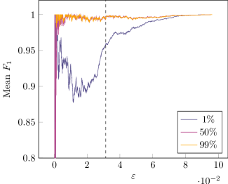
(a)

(b)

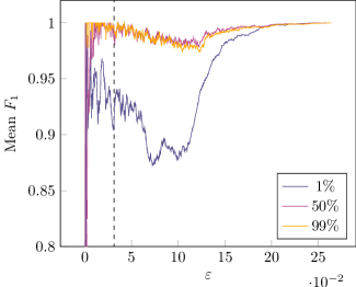
(c)

(d)

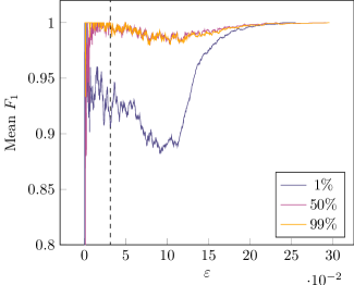
(e)

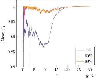
(f)

Figure 3: $F_{1}$ scores in relation to $\varepsilon$ for MNIST A for each considered percentile. For ease of visualization, we set the graph cutoff at $F_{1}=0.8$. We also mark 8/255 (a common choice for $\varepsilon$) with a dotted line.

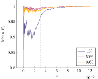
(a)

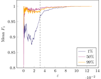
(b)

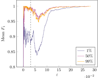
(c)

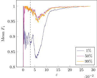
(d)

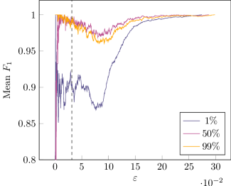
(e)

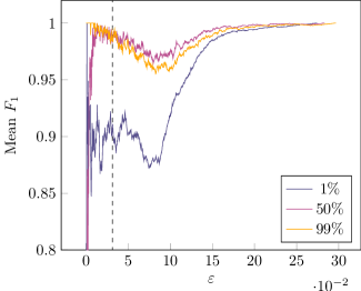
(f)

Figure 4: $F_{1}$ scores in relation to $\varepsilon$ for MNIST B for each considered percentile. For ease of visualization, we set the graph cutoff at $F_{1}=0.8$. We also mark 8/255 (a common choice for $\varepsilon$) with a dotted line.

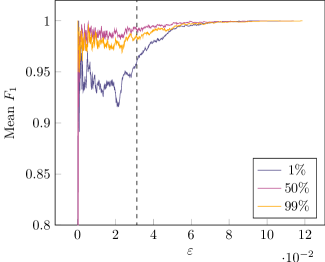
(a)

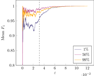
(b)

(c)

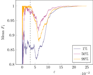
(d)

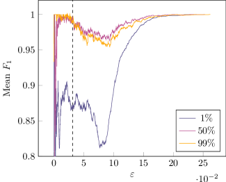
(e)

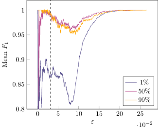
(f)

Figure 5: $F_{1}$ scores in relation to $\varepsilon$ for MNIST C for each considered percentile. For ease of visualization, we set the graph cutoff at $F_{1}=0.8$. We also mark 8/255 (a common choice for $\varepsilon$) with a dotted line.

(a)

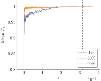
(b)

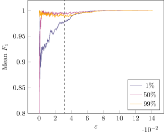
(c)

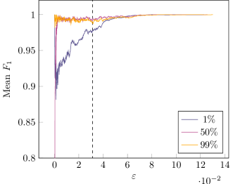
(d)

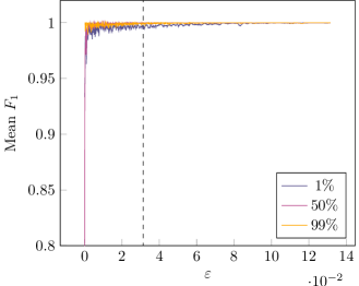
(e)

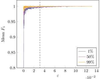
(f)

Figure 6: $F_{1}$ scores in relation to $\varepsilon$ for CIFAR10 A for each considered percentile. For ease of visualization, we set the graph cutoff at $F_{1}=0.8$. We also mark 8/255 (a common choice for $\varepsilon$) with a dotted line.

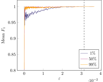
(a)

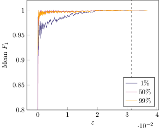
(b)

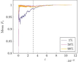
(c)

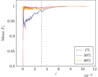
(d)

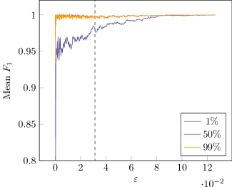
(e)

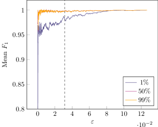
(f)

Figure 7: $F_{1}$ scores in relation to $\varepsilon$ for CIFAR10 B for each considered percentile. For ease of visualization, we set the graph cutoff at $F_{1}=0.8$. We also mark 8/255 (a common choice for $\varepsilon$) with a dotted line.

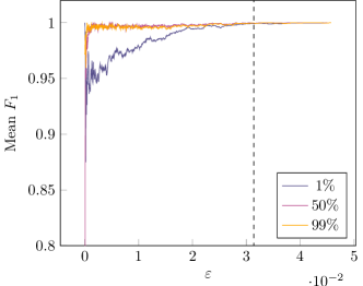
(a)

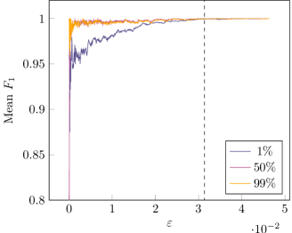
(b)

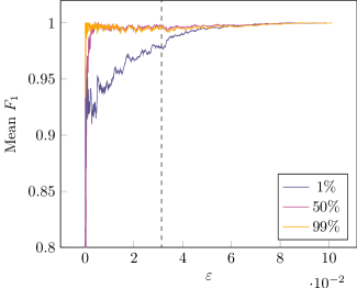
(c)

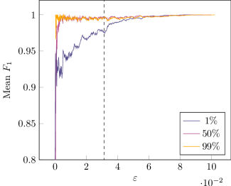
(d)

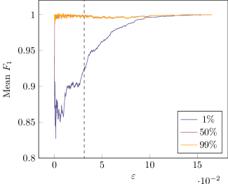
(e)

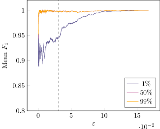
(f)

Figure 8: $F_{1}$ scores in relation to $\varepsilon$ for CIFAR10 C for each considered percentile. For ease of visualization, we set the graph cutoff at $F_{1}=0.8$. We also mark 8/255 (a common choice for $\varepsilon$) with a dotted line.

Appendix J Additional Results

Tables 14, 15, 16 and 17 detail the performance of the various attack sets on every combination, while Figures 9, 10, 11, 12, 13 and 14 showcase the relation between the true and estimated decision boundary distances.

Table 14: Performance of the strong attack set on MNIST.

Architecture	Training	Success Rate	Difference	% Below 1/255	$\mathbf{R^{2}}$
MNIST A	Standard	100.00%	1.51%	98.16%	0.996
	Adversarial	100.00%	2.48%	81.43%	0.994
	ReLU	100.00%	2.14%	84.33%	0.995
MNIST B	Standard	100.00%	3.38%	97.36%	0.995
	Adversarial	100.00%	4.34%	75.09%	0.991
	ReLU	100.00%	4.80%	68.02%	0.992
MNIST C	Standard	100.00%	4.52%	96.92%	0.996
	Adversarial	100.00%	8.76%	48.78%	0.981
	ReLU	100.00%	4.84%	68.24%	0.988

Table 15: Performance of the balanced attack set on MNIST.

Architecture	Training	Success Rate	Difference	% Below 1/255	$\mathbf{R^{2}}$
MNIST A	Standard	100.00%	1.68%	97.94%	0.995
	Adversarial	100.00%	2.87%	77.64%	0.993
	ReLU	100.00%	2.55%	80.86%	0.993
MNIST B	Standard	100.00%	4.09%	96.55%	0.995
	Adversarial	100.00%	4.90%	72.60%	0.988
	ReLU	100.00%	5.53%	62.96%	0.989
MNIST C	Standard	100.00%	5.43%	96.04%	0.995
	Adversarial	100.00%	9.50%	48.43%	0.977
	ReLU	100.00%	5.28%	66.96%	0.986

Table 16: Performance of the strong attack set on CIFAR10.

Architecture	Training	Success Rate	Difference	% Below 1/255	$\mathbf{R^{2}}$
CIFAR10 A	Standard	100.00%	1.62%	100.00%	0.999
	Adversarial	100.00%	4.42%	95.88%	0.995
	ReLU	100.00%	0.26%	100.00%	1.000
CIFAR10 B	Standard	100.00%	1.44%	100.00%	0.999
	Adversarial	100.00%	3.17%	97.69%	0.997
	ReLU	100.00%	1.38%	98.81%	0.999
CIFAR10 C	Standard	100.00%	2.11%	100.00%	0.999
	Adversarial	100.00%	3.10%	97.14%	0.996
	ReLU	100.00%	2.35%	96.12%	0.990

Table 17: Performance of the balanced attack set on CIFAR10.

Architecture	Training	Success Rate	Difference	% Below 1/255	$\mathbf{R^{2}}$
CIFAR10 A	Standard	100.00%	1.71%	100.00%	0.999
	Adversarial	100.00%	4.18%	96.57%	0.995
	ReLU	100.00%	0.18%	100.00%	1.000
CIFAR10 B	Standard	100.00%	1.53%	100.00%	0.999
	Adversarial	100.00%	2.92%	98.46%	0.996
	ReLU	100.00%	1.19%	98.94%	0.999
CIFAR10 C	Standard	100.00%	2.06%	100.00%	0.999
	Adversarial	100.00%	3.12%	97.28%	0.996
	ReLU	100.00%	1.45%	97.44%	0.995

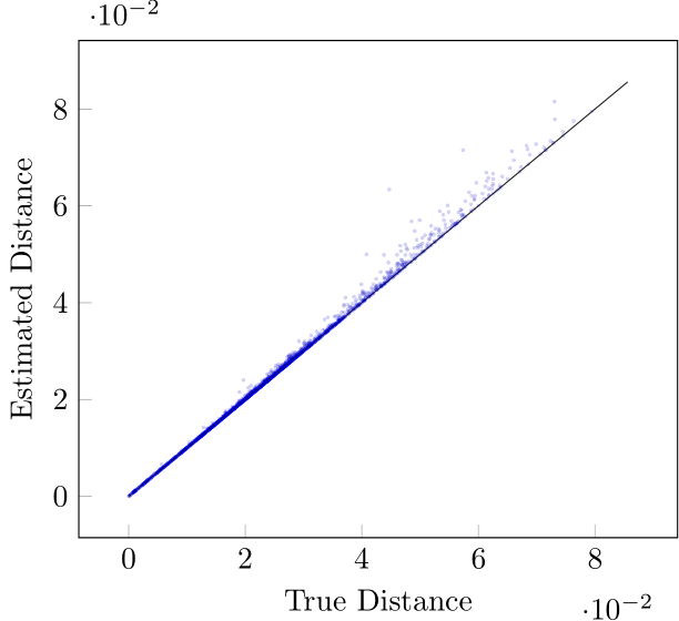
(a)

(b)

(c)

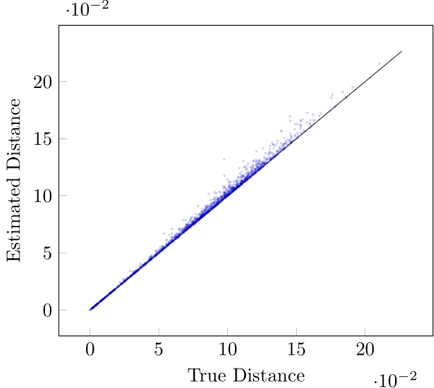
(d)

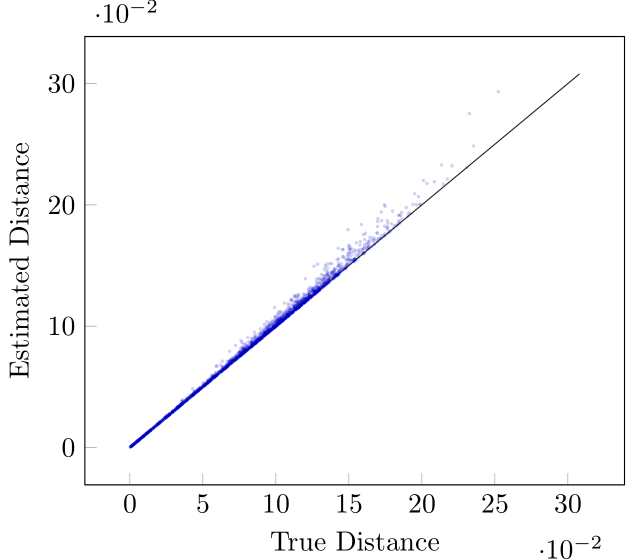
(e)

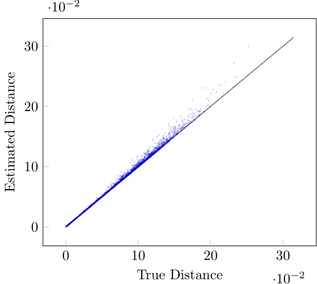
(f)

Figure 9: Decision boundary distances found by the attack pools compared to those found by MIPVerify on MNIST A. The black line represents the theoretical optimum. Note that no samples are below the black line.

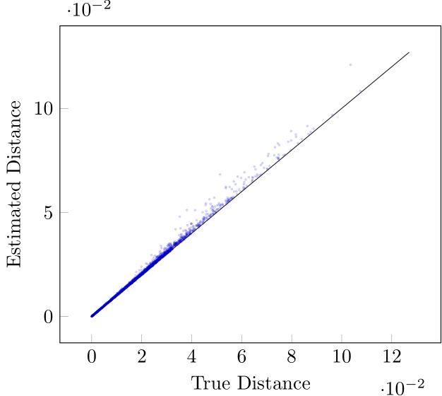
(a)

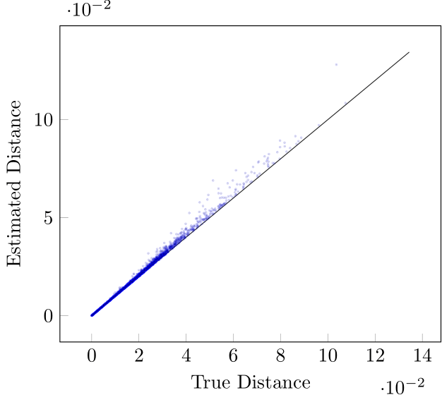
(b)

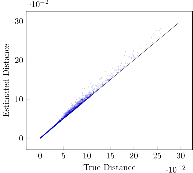
(c)

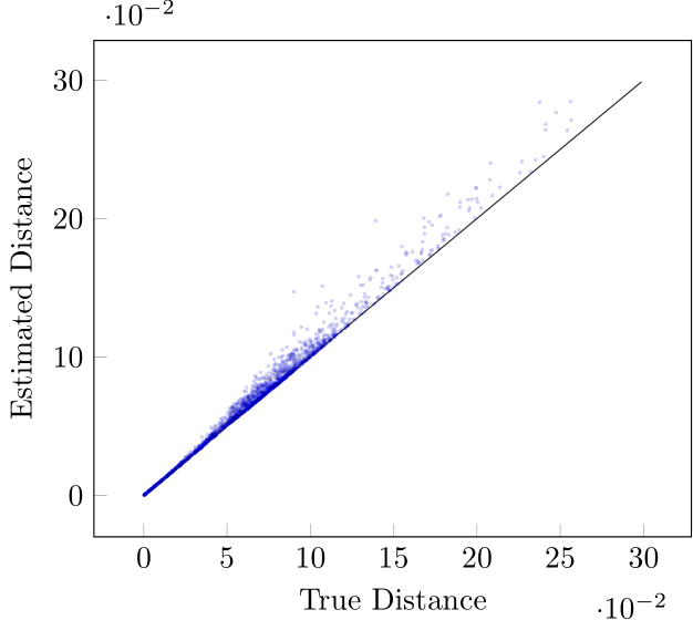
(d)

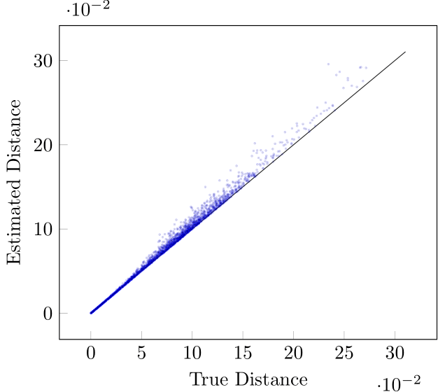
(e)

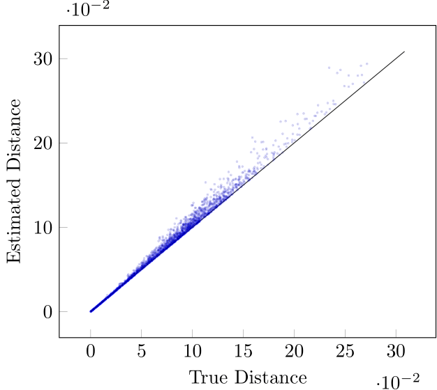
(f)

Figure 10: Decision boundary distances found by the attack pools compared to those found by MIPVerify on MNIST B. The black line represents the theoretical optimum. Note that no samples are below the black line.

(a)

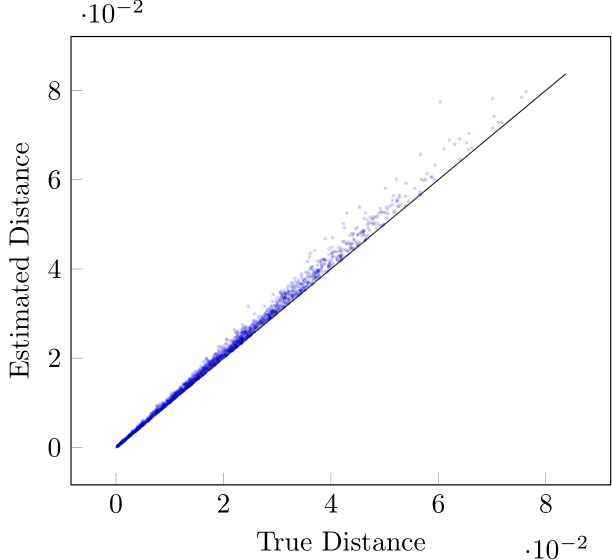
(b)

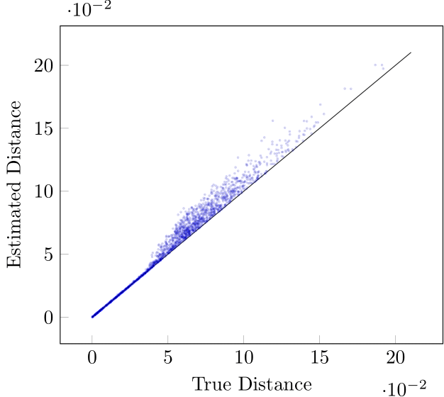
(c)

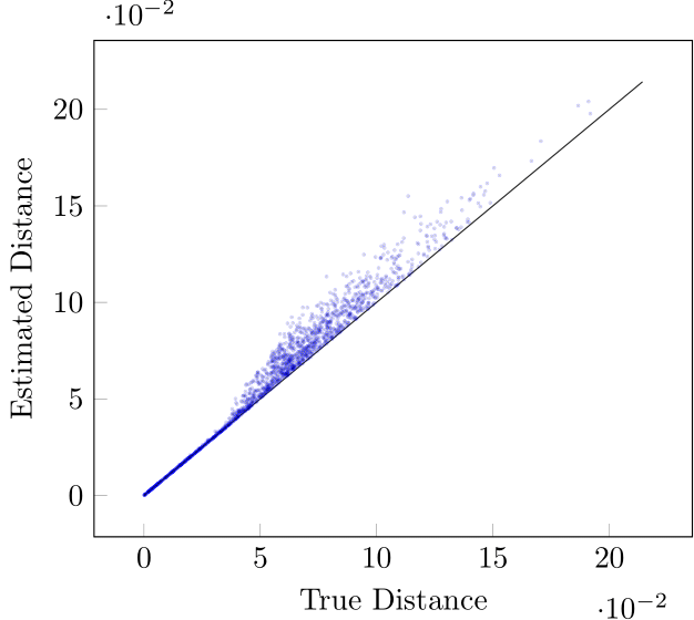
(d)

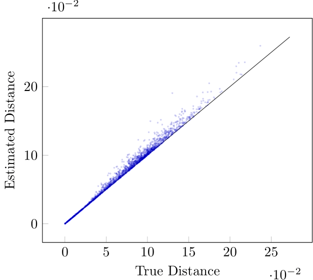
(e)

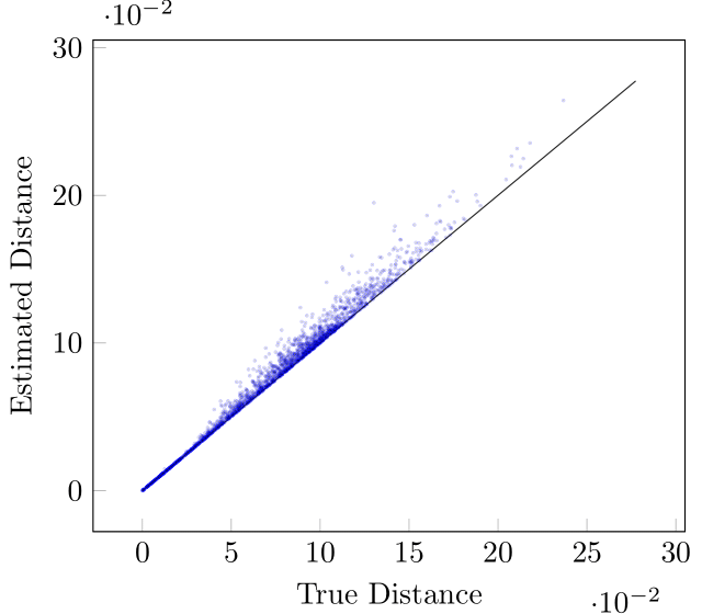
(f)

Figure 11: Decision boundary distances found by the attack pools compared to those found by MIPVerify on MNIST C. The black line represents the theoretical optimum. Note that no samples are below the black line.

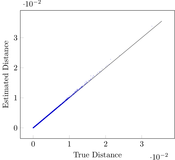
(a)

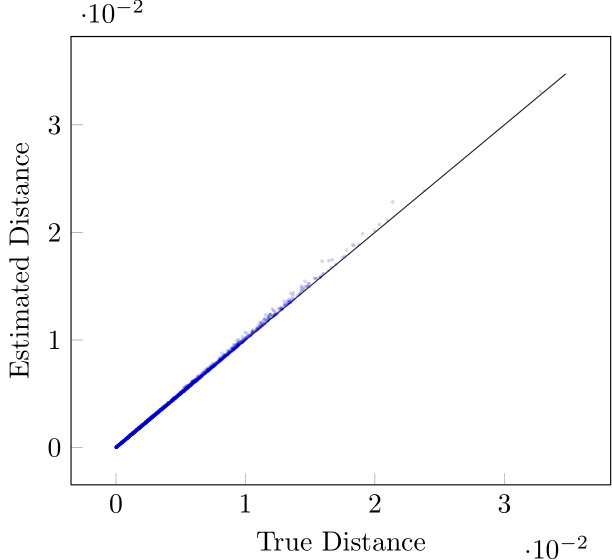
(b)

(c)

(d)

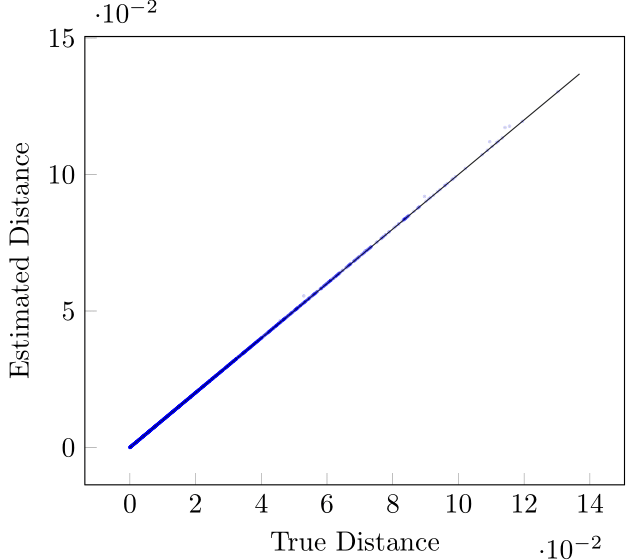
(e)

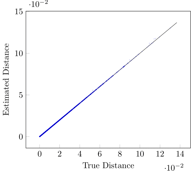
(f)

Figure 12: Decision boundary distances found by the attack pools compared to those found by MIPVerify on CIFAR10 A. The black line represents the theoretical optimum. Note that no samples are below the black line.

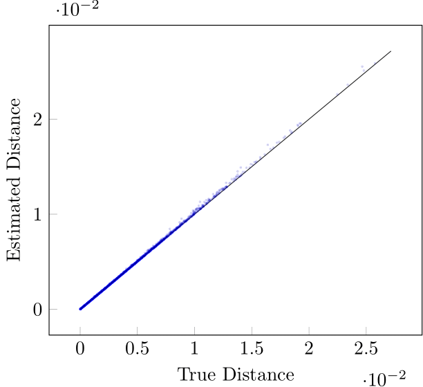
(a)

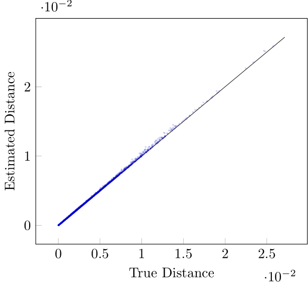
(b)

(c)

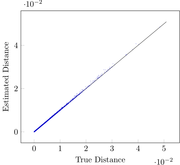
(d)

(e)

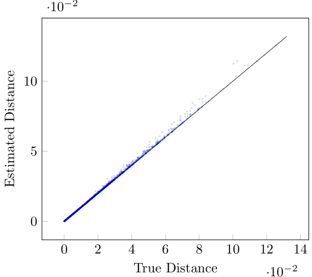
(f)

Figure 13: Decision boundary distances found by the attack pools compared to those found by MIPVerify on CIFAR10 B. The black line represents the theoretical optimum. Note that no samples are below the black line.

(a)

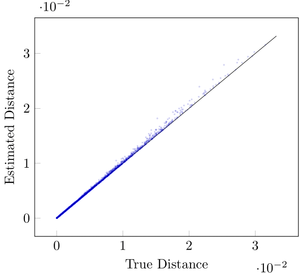
(b)

(c)

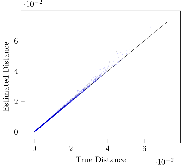
(d)

(e)

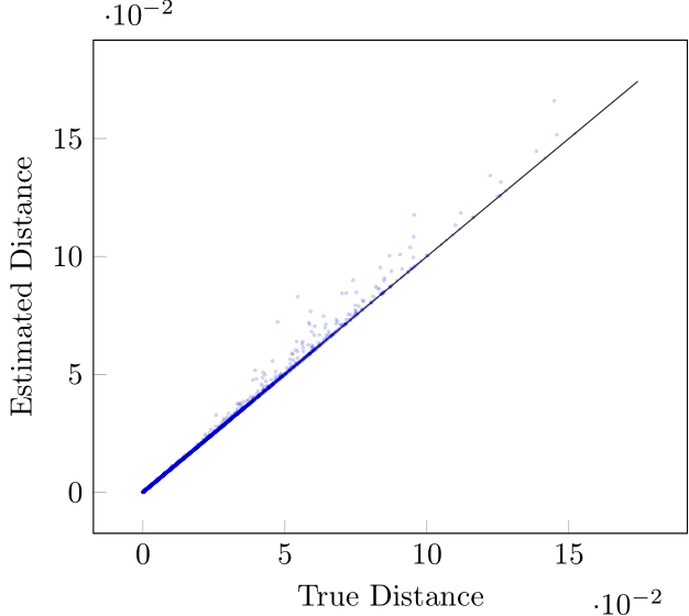
(f)

Figure 14: Decision boundary distances found by the attack pools compared to those found by MIPVerify on CIFAR10 C. The black line represents the theoretical optimum. Note that no samples are below the black line.

Appendix K Ablation Study

We outline the best attack pools by size in Tables 18, 19, 20 and 21. Additionally, we report the performance of pools composed of individual attacks in Tables 22, 23, 24 and 25. Finally, we detail the performance of dropping a specific attack in Tables 26, 27, 28 and 29.

Table 18: Best pools of a given size by success rate and $R^{2}$ for MNIST strong.

$\bm{n}$	Attacks	Success Rate	Difference	$\mathbf{<}$ 1/255	$\mathbf{R^{2}}$
1	PGD	100.00±0.00%	10.98±4.41%	51.83±27.78%	0.975±0.010
2	C&W, PGD	100.00±0.00%	7.99±3.31%	60.68±25.43%	0.986±0.005
3	B&B, C&W, PGD	100.00±0.00%	4.71±1.97%	77.97±15.52%	0.989±0.004
4	B&B, C&W, DF, PGD	100.00±0.00%	4.36±2.03%	79.02±15.62%	0.991±0.005
5	No FGSM, Uniform	100.00±0.00%	4.09±2.02%	79.81±15.70%	0.992±0.005
6	No Uniform	100.00±0.00%	4.09±2.02%	79.81±15.70%	0.992±0.005
7	All	100.00±0.00%	4.09±2.02%	79.81±15.70%	0.992±0.005

Table 19: Best pools of a given size by success rate and $R^{2}$ for MNIST balanced.

$\bm{n}$	Attacks	Success Rate	Difference	$\mathbf{<}$ 1/255	$\mathbf{R^{2}}$
1	BIM	100.00±0.00%	11.72±4.18%	50.92±26.43%	0.965±0.010
2	BIM, B&B	100.00±0.00%	6.11±2.28%	73.23±15.90%	0.980±0.007
3	BIM, B&B, C&W	100.00±0.00%	5.29±2.06%	75.72±16.10%	0.986±0.005
4	BIM, B&B, C&W, DF	100.00±0.00%	4.85±2.10%	77.33±15.85%	0.989±0.005
5	No FGSM, Uniform	100.00±0.00%	4.65±2.16%	77.78±16.08%	0.990±0.006
6	No Uniform	100.00±0.00%	4.65±2.16%	77.78±16.08%	0.990±0.006
7	All	100.00±0.00%	4.65±2.16%	77.78±16.08%	0.990±0.006

Table 20: Best pools of a given size by success rate and $R^{2}$ for CIFAR10 strong.

$\bm{n}$	Attacks	Success Rate	Difference	$\mathbf{<}$ 1/255	$\mathbf{R^{2}}$
1	DF	100.00±0.00%	6.11±3.49%	95.06±4.81%	0.989±0.011
2	DF, PGD	100.00±0.00%	4.71±2.37%	96.32±3.56%	0.995±0.007
3	C&W, DF, PGD	100.00±0.00%	2.54±1.30%	98.17±2.00%	0.996±0.006
4	B&B, C&W, DF, PGD	100.00±0.00%	2.21±1.16%	98.40±1.63%	0.997±0.003
5	No FGSM, Uniform	100.00±0.00%	2.21±1.16%	98.40±1.63%	0.997±0.003
6	No Uniform	100.00±0.00%	2.21±1.16%	98.40±1.63%	0.997±0.003
7	All	100.00±0.00%	2.21±1.16%	98.40±1.63%	0.997±0.003

Table 21: Best pools of a given size by success rate and $R^{2}$ for CIFAR10 balanced.

$\bm{n}$	Attacks	Success Rate	Difference	$\mathbf{<}$ 1/255	$\mathbf{R^{2}}$
1	DF	100.00±0.00%	6.11±3.49%	95.06±4.81%	0.989±0.011
2	B&B, DF	100.00±0.00%	2.52±1.51%	98.23±1.81%	0.995±0.004
3	BIM, B&B, DF	100.00±0.00%	2.21±1.25%	98.53±1.52%	0.997±0.002
4	BIM, B&B, C&W, DF	100.00±0.00%	2.06±1.16%	98.73±1.32%	0.998±0.002
5	No FGSM, Uniform	100.00±0.00%	2.04±1.13%	98.74±1.29%	0.998±0.002
6	No FGSM	100.00±0.00%	2.04±1.13%	98.74±1.29%	0.998±0.002
7	All	100.00±0.00%	2.04±1.13%	98.74±1.29%	0.998±0.002

Table 22: Performance of individual attacks for MNIST strong.

Attack	Success Rate	Difference	$\mathbf{<}$ 1/255	$\mathbf{R^{2}}$
BIM	100.00±0.00%	10.90±4.42%	53.57±28.07%	0.966±0.012
B&B	99.99±0.01%	18.50±7.09%	58.78±9.91%	0.812±0.044
C&W	100.00±0.00%	17.52±2.74%	48.02±21.28%	0.910±0.024
Deepfool	100.00±0.00%	21.59±7.73%	44.15±20.02%	0.923±0.027
FGSM	99.72±0.51%	44.43±15.76%	28.20±17.30%	0.761±0.132
PGD	100.00±0.00%	10.98±4.41%	51.83±27.78%	0.975±0.010
Uniform	99.52±0.91%	414.47±140.54%	0.82±0.55%	0.623±0.138

Table 23: Performance of individual attacks for MNIST balanced.

Attack	Success Rate	Difference	$\mathbf{<}$ 1/255	$\mathbf{R^{2}}$
BIM	100.00±0.00%	11.72±4.18%	50.92±26.43%	0.965±0.010
B&B	99.99±0.03%	18.65±7.29%	58.43±9.61%	0.812±0.039
C&W	100.00±0.00%	22.55±3.83%	38.95±22.49%	0.904±0.025
Deepfool	100.00±0.00%	21.59±7.73%	44.15±20.02%	0.923±0.027
FGSM	99.72±0.51%	44.43±15.76%	28.20±17.30%	0.761±0.132
PGD	100.00±0.00%	16.23±6.59%	48.08±28.88%	0.905±0.070
Uniform	98.66±1.90%	521.61±181.40%	0.57±0.38%	0.484±0.122

Table 24: Performance of individual attacks for CIFAR10 strong.

Attack	Success Rate	Difference	$\mathbf{<}$ 1/255	$\mathbf{R^{2}}$
BIM	91.96±7.40%	19.97±5.95%	80.32±12.97%	0.934±0.041
B&B	100.00±0.00%	508.66±196.37%	42.74±7.85%	0.174±0.074
C&W	99.98±0.02%	10.67±3.64%	90.09±5.51%	0.926±0.030
Deepfool	100.00±0.00%	6.11±3.49%	95.06±4.81%	0.989±0.011
FGSM	100.00±0.00%	31.80±11.12%	69.20±17.72%	0.847±0.123
PGD	100.00±0.00%	19.36±5.99%	77.23±15.89%	0.952±0.027
Uniform	99.99±0.02%	1206.79±277.68%	2.48±0.88%	0.910±0.044

Table 25: Performance of individual attacks for CIFAR10 balanced.

Attack	Success Rate	Difference	$\mathbf{<}$ 1/255	$\mathbf{R^{2}}$
BIM	100.00±0.00%	19.23±5.92%	77.33±15.89%	0.954±0.025
B&B	100.00±0.00%	50.64±52.17%	81.20±10.68%	0.615±0.349
C&W	99.89±0.09%	17.44±4.01%	84.82±8.51%	0.923±0.026
Deepfool	100.00±0.00%	6.11±3.49%	95.06±4.81%	0.989±0.011
FGSM	100.00±0.00%	31.80±11.12%	69.20±17.72%	0.847±0.123
PGD	100.00±0.00%	20.18±6.56%	76.97±16.07%	0.947±0.031
Uniform	99.85±0.26%	1617.74±390.50%	1.80±0.67%	0.853±0.068

Table 26: Performance of pools without a specific attack for MNIST strong.

Dropped Attack	Success Rate	Difference	$\mathbf{<}$ 1/255	$\mathbf{R^{2}}$
None	100.00±0.00%	4.09±2.02%	79.81±15.70%	0.992±0.005
BIM	100.00±0.00%	4.35±2.03%	79.02±15.62%	0.991±0.005
B&B	100.00±0.00%	6.76±3.31%	64.46±25.01%	0.990±0.005
C&W	100.00±0.00%	4.65±2.20%	77.70±16.02%	0.989±0.006
Deepfool	100.00±0.00%	4.33±1.97%	79.04±15.75%	0.990±0.004
FGSM	100.00±0.00%	4.09±2.02%	79.81±15.70%	0.992±0.005
PGD	100.00±0.00%	4.26±1.99%	79.36±15.59%	0.991±0.004
Uniform	100.00±0.00%	4.09±2.02%	79.81±15.70%	0.992±0.005

Table 27: Performance of pools without a specific attack for MNIST balanced.

Dropped Attack	Success Rate	Difference	$\mathbf{<}$ 1/255	$\mathbf{R^{2}}$
None	100.00±0.00%	4.65±2.16%	77.78±16.08%	0.990±0.006
BIM	100.00±0.00%	5.13±2.27%	76.14±15.98%	0.988±0.007
B&B	100.00±0.00%	7.93±3.69%	60.79±25.99%	0.987±0.006
C&W	100.00±0.00%	4.93±2.22%	77.05±15.96%	0.988±0.006
Deepfool	100.00±0.00%	5.03±2.14%	76.34±16.36%	0.988±0.005
FGSM	100.00±0.00%	4.65±2.16%	77.78±16.08%	0.990±0.006
PGD	100.00±0.00%	4.85±2.10%	77.33±15.85%	0.989±0.005
Uniform	100.00±0.00%	4.65±2.16%	77.78±16.08%	0.990±0.006

Table 28: Performance of pools without a specific attack for CIFAR10 strong.

Dropped Attack	Success Rate	Difference	$\mathbf{<}$ 1/255	$\mathbf{R^{2}}$
None	100.00±0.00%	2.21±1.16%	98.40±1.63%	0.997±0.003
BIM	100.00±0.00%	2.21±1.16%	98.40±1.63%	0.997±0.003
B&B	100.00±0.00%	2.54±1.30%	98.17±2.00%	0.996±0.006
C&W	100.00±0.00%	3.83±2.06%	96.84±3.12%	0.996±0.004
Deepfool	100.00±0.00%	4.02±1.19%	95.65±3.10%	0.992±0.005
FGSM	100.00±0.00%	2.21±1.16%	98.40±1.63%	0.997±0.003
PGD	100.00±0.00%	2.50±1.48%	98.11±1.93%	0.995±0.005
Uniform	100.00±0.00%	2.21±1.16%	98.40±1.63%	0.997±0.003

Table 29: Performance of pools without a specific attack for CIFAR10 balanced.

Dropped Attack	Success Rate	Difference	$\mathbf{<}$ 1/255	$\mathbf{R^{2}}$
None	100.00±0.00%	2.04±1.13%	98.74±1.29%	0.998±0.002
BIM	100.00±0.00%	2.07±1.15%	98.72±1.31%	0.998±0.002
B&B	100.00±0.00%	4.08±1.95%	97.26±2.70%	0.996±0.006
C&W	100.00±0.00%	2.18±1.22%	98.54±1.50%	0.997±0.002
Deepfool	100.00±0.00%	4.00±0.99%	95.89±3.13%	0.993±0.003
FGSM	100.00±0.00%	2.04±1.13%	98.74±1.29%	0.998±0.002
PGD	100.00±0.00%	2.06±1.16%	98.73±1.32%	0.998±0.002
Uniform	100.00±0.00%	2.04±1.13%	98.74±1.29%	0.998±0.002

Appendix L Fast Parameter Set Tests

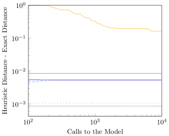
(a) MNIST C Standard Fast-100

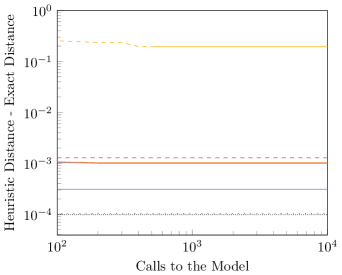
(b) CIFAR10 C Standard Fast-100

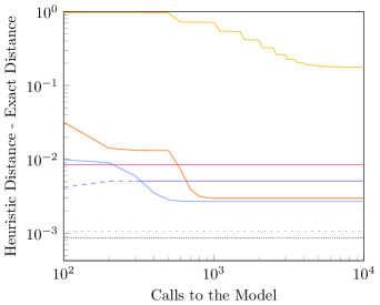
(c) MNIST C Standard Fast-1k

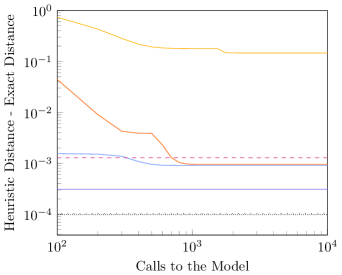
(d) CIFAR10 C Standard Fast-1k

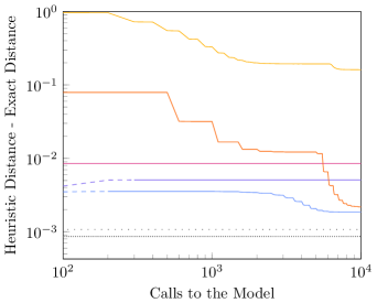
(e) MNIST C Standard Fast-10k

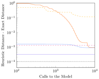
(f) CIFAR10 C Standard Fast-10k

Figure 21: Mean difference between the distance of the closest adversarial examples and the exact decision boundary distance for MNIST & CIFAR10 C Standard. A dashed line means that the attack found adversarial examples (of any distance) for only some inputs, while the absence of a line means that the attack did not find any adversarial examples. The loosely and densely dotted black lines respectively represent the balanced and strong attack pools. Both axes are logarithmic.

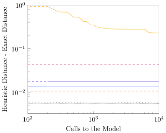
(a) MNIST C Adversarial Fast-100

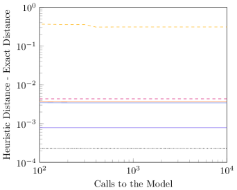
(b) CIFAR10 C Adversarial Fast-100

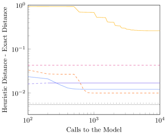
(c) MNIST C Adversarial Fast-1k

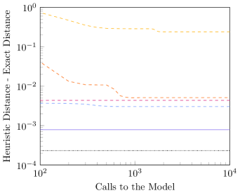
(d) CIFAR10 C Adversarial Fast-1k

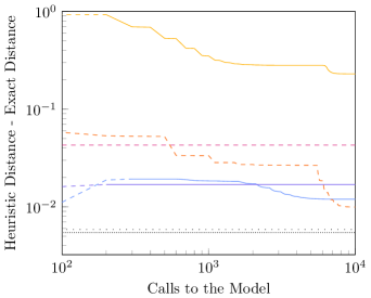
(e) MNIST C Adversarial Fast-10k

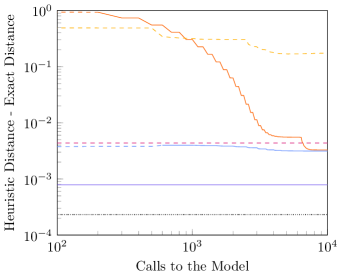
(f) CIFAR10 C Adversarial Fast-10k

Figure 22: Mean difference between the distance of the closest adversarial examples and the exact decision boundary distance for MNIST & CIFAR10 C Adversarial. A dashed line means that the attack found adversarial examples (of any distance) for only some inputs, while the absence of a line means that the attack did not find any adversarial examples. The loosely and densely dotted black lines respectively represent the balanced and strong attack pools. Both axes are logarithmic.

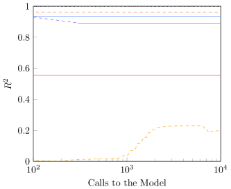
(a) MNIST A Standard Fast-100

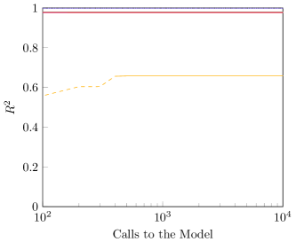
(b) CIFAR10 A Standard Fast-100

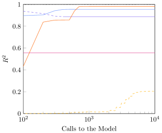
(c) MNIST A Standard Fast-1k

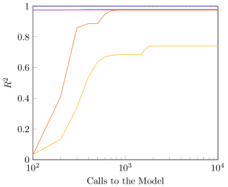
(d) CIFAR10 A Standard Fast-1k

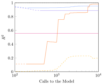
(e) MNIST A Standard Fast-10k

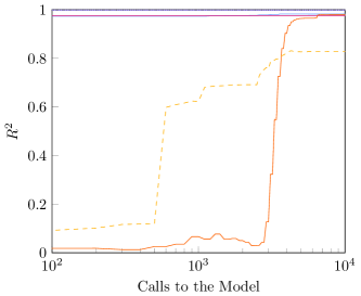
(f) CIFAR10 A Standard Fast-10k

Figure 24: $R^{2}$ of linear model for the heuristic adversarial distances given the exact decision boundary distances for MNIST & CIFAR10 A Standard. A dashed line means that the attack found adversarial examples (of any distance) for only some inputs, while the absence of a line means that the attack did not find any adversarial examples. The loosely and densely dotted black lines respectively represent the balanced and strong attack pools. The x axis is logarithmic.

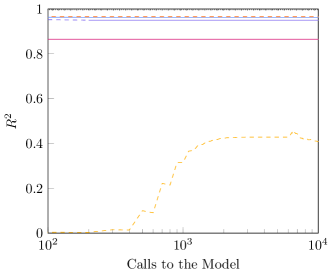
(a) MNIST A Adversarial Fast-100

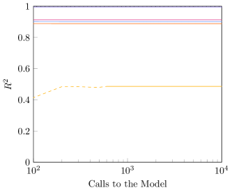
(b) CIFAR10 A Adversarial Fast-100

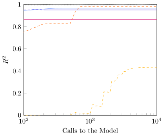
(c) MNIST A Adversarial Fast-1k

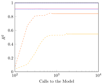
(d) CIFAR10 A Adversarial Fast-1k

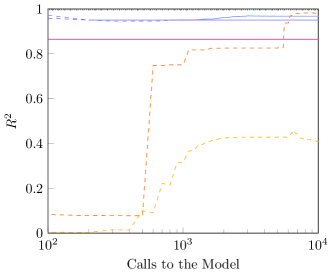
(e) MNIST A Adversarial Fast-10k

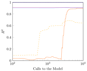
(f) CIFAR10 A Adversarial Fast-10k

Figure 25: $R^{2}$ of linear model for the heuristic adversarial distances given the exact decision boundary distances for MNIST & CIFAR10 A Adversarial. A dashed line means that the attack found adversarial examples (of any distance) for only some inputs, while the absence of a line means that the attack did not find any adversarial examples. The loosely and densely dotted black lines respectively represent the balanced and strong attack pools. The x axis is logarithmic.

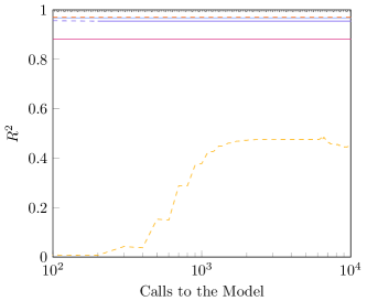
(a) MNIST A ReLU Fast-100

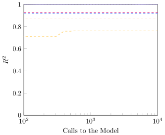
(b) CIFAR10 A ReLU Fast-100

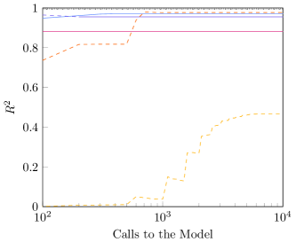
(c) MNIST A ReLU Fast-1k

(d) CIFAR10 A ReLU Fast-1k

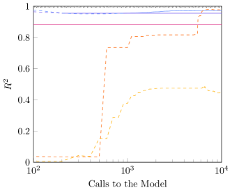
(e) MNIST A ReLU Fast-10k

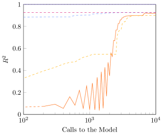
(f) CIFAR10 A ReLU Fast-10k

Figure 26: $R^{2}$ of linear model for the heuristic adversarial distances given the exact decision boundary distances for MNIST & CIFAR10 A ReLU. A dashed line means that the attack found adversarial examples (of any distance) for only some inputs, while the absence of a line means that the attack did not find any adversarial examples. The loosely and densely dotted black lines respectively represent the balanced and strong attack pools. The x axis is logarithmic.

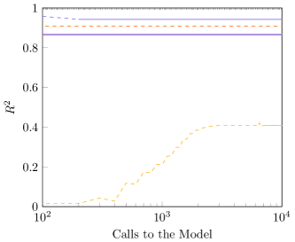
(a) MNIST B Standard Fast-100

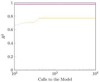
(b) CIFAR10 B Standard Fast-100

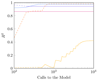
(c) MNIST B Standard Fast-1k

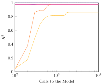
(d) CIFAR10 B Standard Fast-1k

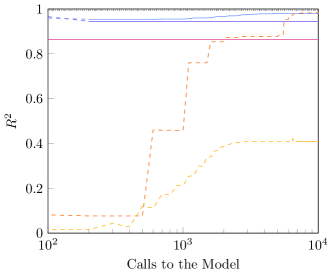
(e) MNIST B Standard Fast-10k

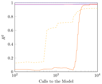
(f) CIFAR10 B Standard Fast-10k

Figure 27: $R^{2}$ of linear model for the heuristic adversarial distances given the exact decision boundary distances for MNIST & CIFAR10 B Standard. A dashed line means that the attack found adversarial examples (of any distance) for only some inputs, while the absence of a line means that the attack did not find any adversarial examples. The loosely and densely dotted black lines respectively represent the balanced and strong attack pools. The x axis is logarithmic.

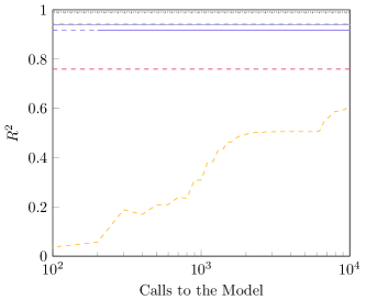
(a) MNIST B Adversarial Fast-100

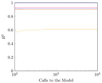
(b) CIFAR10 B Adversarial Fast-100

(c) MNIST B Adversarial Fast-1k

(d) CIFAR10 B Adversarial Fast-1k

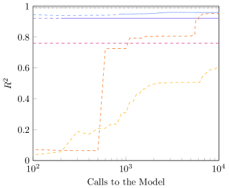
(e) MNIST B Adversarial Fast-10k

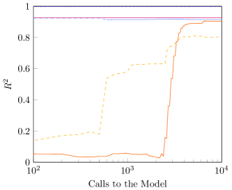
(f) CIFAR10 B Adversarial Fast-10k

Figure 28: $R^{2}$ of linear model for the heuristic adversarial distances given the exact decision boundary distances for MNIST & CIFAR10 B Adversarial. A dashed line means that the attack found adversarial examples (of any distance) for only some inputs, while the absence of a line means that the attack did not find any adversarial examples. The loosely and densely dotted black lines respectively represent the balanced and strong attack pools. The x axis is logarithmic.

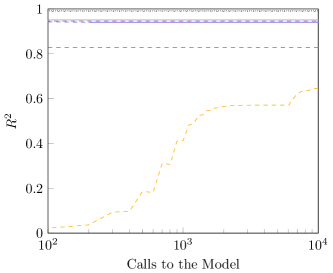
(a) MNIST B ReLU Fast-100

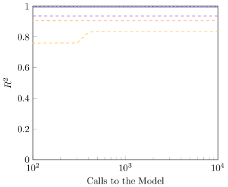
(b) CIFAR10 B ReLU Fast-100

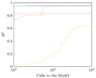
(c) MNIST B ReLU Fast-1k

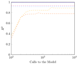
(d) CIFAR10 B ReLU Fast-1k

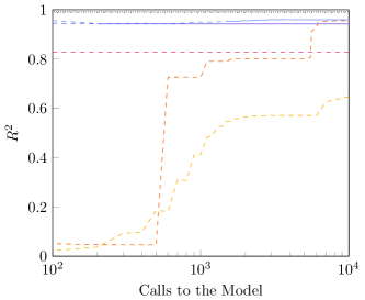
(e) MNIST B ReLU Fast-10k

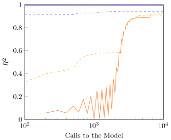
(f) CIFAR10 B ReLU Fast-10k

Figure 29: $R^{2}$ of linear model for the heuristic adversarial distances given the exact decision boundary distances for MNIST & CIFAR10 B ReLU. A dashed line means that the attack found adversarial examples (of any distance) for only some inputs, while the absence of a line means that the attack did not find any adversarial examples. The loosely and densely dotted black lines respectively represent the balanced and strong attack pools. The x axis is logarithmic.

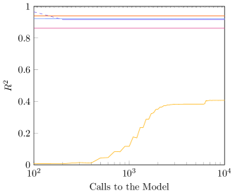
(a) MNIST C Standard Fast-100

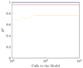
(b) CIFAR10 C Standard Fast-100

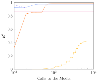
(c) MNIST C Standard Fast-1k

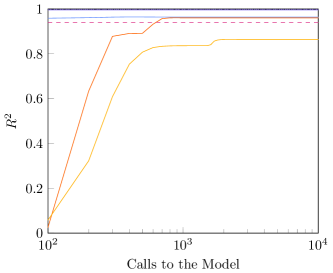
(d) CIFAR10 C Standard Fast-1k

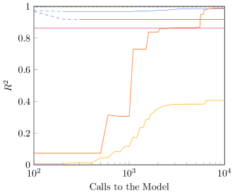
(e) MNIST C Standard Fast-10k

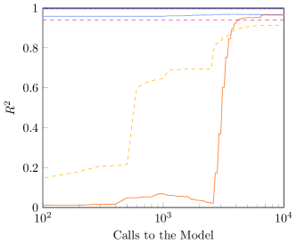
(f) CIFAR10 C Standard Fast-10k

Figure 30: $R^{2}$ of linear model for the heuristic adversarial distances given the exact decision boundary distances for MNIST & CIFAR10 C Standard. A dashed line means that the attack found adversarial examples (of any distance) for only some inputs, while the absence of a line means that the attack did not find any adversarial examples. The loosely and densely dotted black lines respectively represent the balanced and strong attack pools. The x axis is logarithmic.

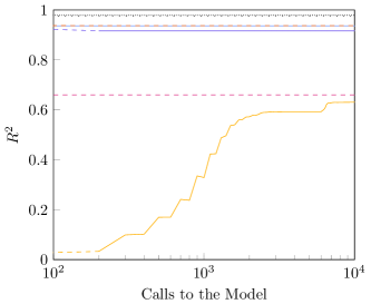
(a) MNIST C Adversarial Fast-100

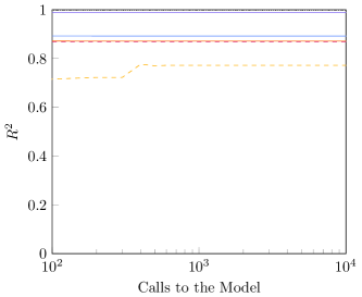
(b) CIFAR10 C Adversarial Fast-100

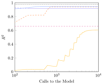
(c) MNIST C Adversarial Fast-1k

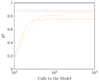
(d) CIFAR10 C Adversarial Fast-1k

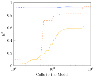
(e) MNIST C Adversarial Fast-10k

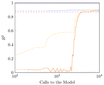
(f) CIFAR10 C Adversarial Fast-10k

Figure 31: $R^{2}$ of linear model for the heuristic adversarial distances given the exact decision boundary distances for MNIST & CIFAR10 C Adversarial. A dashed line means that the attack found adversarial examples (of any distance) for only some inputs, while the absence of a line means that the attack did not find any adversarial examples. The loosely and densely dotted black lines respectively represent the balanced and strong attack pools. The x axis is logarithmic.

We list the chosen parameter sets for Fast-100, Fast-1k and Fast-10k in Table 30. We plot the difference between the distance of the closest adversarial examples and the true decision boundary distance in Figures 15, 16, 17, 18, 19, 20, 21, 22 and 23, while we plot the $R^{2}$ values in Figures 24, 25, 26, 27, 28, 29, 30, 31 and 32. We do not study the Brendel & Bethge and the Carlini & Wagner attacks due to the fact that the number of model calls varies depending on how many inputs are attacked at the same time. Note that, for attacks that do not have the a 100% success rate, the mean adversarial example distance can increase with the number of steps as new adversarial examples (for inputs for which there were previously no successful adversarial examples) are added.

Table 30: Parameters for the Fast-100, Fast-1k and Fast-10k sets.

Attack	Parameter Name	MNIST			CIFAR10
		100	1k	10k	100	1k	10k
BIM	Initial Search Factor	N/A
	Initial Search Steps	N/A
	Binary Search Steps	10	20	20	10	20	20
	Starting $\varepsilon$	0.5			0.1
	#Iterations	10	50	500	10	50	500
	Learning Rate	0.1	0.01	1e-3	0.01	1e-3	1e-3
Deepfool	#Iterations	100	500	500	500
	Candidates	10
	Overshoot	0.1	1e-5	1e-5	1e-4
	Loss	Logits
FGSM	Initial Search Factor	0.75			0.5
	Initial Search Steps	30			10
	Binary Search Steps	20
	Starting $\varepsilon$	1			0.1
PGD	Initial Search Factor	N/A	0.5	0.5	N/A	0.5	0.75
	Initial Search Steps	N/A	10	10	N/A	10	30
	Binary Search Steps	10			10	10	20
	Starting $\varepsilon$	0.1			0.1	0.1	1
	#Iterations	10	50	500	10	50	200
	Learning Rate	0.1	0.01	1e-3	0.01	1e-3	1e-3
	Random Initialization	True
Uniform Noise	Initial Search Factor	0.75			0.75	0.75	0.25
	Initial Search Steps	30			30	30	5
	Binary Search Steps	20			20	20	15
	Starting $\varepsilon$	1			1	1	0.5
	Runs	200	500	200	10	50	500

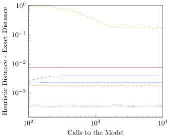
(a) MNIST A Standard Fast-100

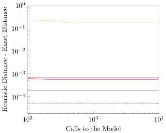
(b) CIFAR10 A Standard Fast-100

(c) MNIST A Standard Fast-1k

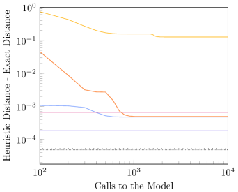
(d) CIFAR10 A Standard Fast-1k

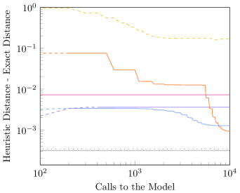
(e) MNIST A Standard Fast-10k

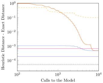
(f) CIFAR10 A Standard Fast-10k

Figure 15: Mean difference between the distance of the closest adversarial examples and the exact decision boundary distance for MNIST & CIFAR10 A Standard. A dashed line means that the attack found adversarial examples (of any distance) for only some inputs, while the absence of a line means that the attack did not find any adversarial examples. The loosely and densely dotted black lines respectively represent the balanced and strong attack pools. Both axes are logarithmic.

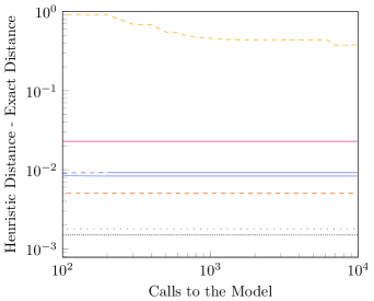
(a) MNIST A Adversarial Fast-100

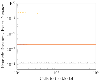
(b) CIFAR10 A Adversarial Fast-100

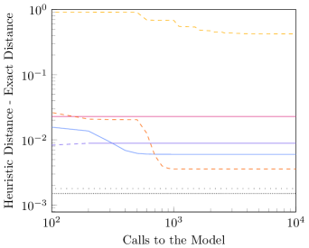
(c) MNIST A Adversarial Fast-1k

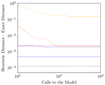
(d) CIFAR10 A Adversarial Fast-1k

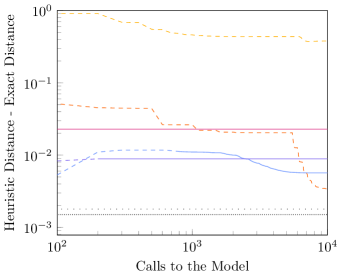
(e) MNIST A Adversarial Fast-10k

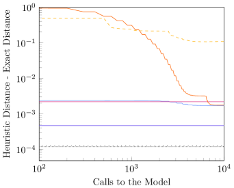
(f) CIFAR10 A Adversarial Fast-10k

Figure 16: Mean difference between the distance of the closest adversarial examples and the exact decision boundary distance for MNIST & CIFAR10 A Adversarial. A dashed line means that the attack found adversarial examples (of any distance) for only some inputs, while the absence of a line means that the attack did not find any adversarial examples. The loosely and densely dotted black lines respectively represent the balanced and strong attack pools. Both axes are logarithmic.

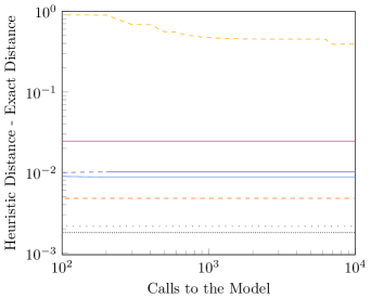
(a) MNIST A ReLU Fast-100

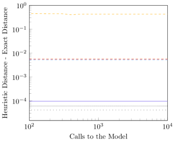
(b) CIFAR10 A ReLU Fast-100

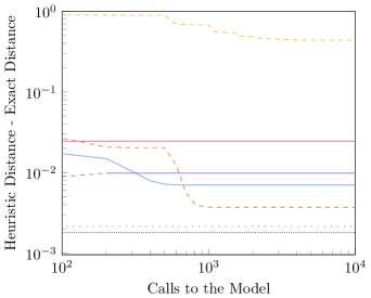
(c) MNIST A ReLU Fast-1k

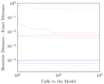
(d) CIFAR10 A ReLU Fast-1k

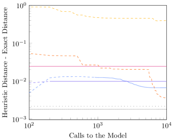
(e) MNIST A ReLU Fast-10k

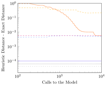
(f) CIFAR10 A ReLU Fast-10k

Figure 17: Mean difference between the distance of the closest adversarial examples and the exact decision boundary distance for MNIST & CIFAR10 A ReLU. A dashed line means that the attack found adversarial examples (of any distance) for only some inputs, while the absence of a line means that the attack did not find any adversarial examples. The loosely and densely dotted black lines respectively represent the balanced and strong attack pools. Both axes are logarithmic.

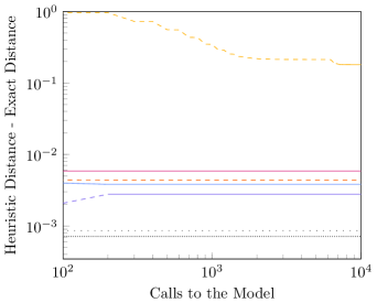
(a) MNIST B Standard Fast-100

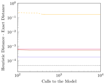
(b) CIFAR10 B Standard Fast-100

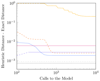
(c) MNIST B Standard Fast-1k

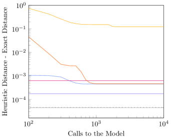
(d) CIFAR10 B Standard Fast-1k

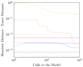
(e) MNIST B Standard Fast-10k

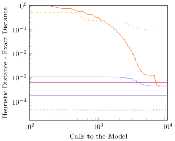
(f) CIFAR10 B Standard Fast-10k

Figure 18: Mean difference between the distance of the closest adversarial examples and the exact decision boundary distance for MNIST & CIFAR10 B Standard. A dashed line means that the attack found adversarial examples (of any distance) for only some inputs, while the absence of a line means that the attack did not find any adversarial examples. The loosely and densely dotted black lines respectively represent the balanced and strong attack pools. Both axes are logarithmic.

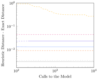
(a) MNIST B Adversarial Fast-100

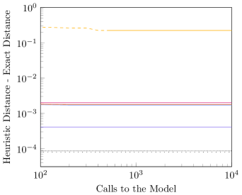
(b) CIFAR10 B Adversarial Fast-100

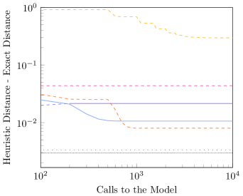
(c) MNIST B Adversarial Fast-1k

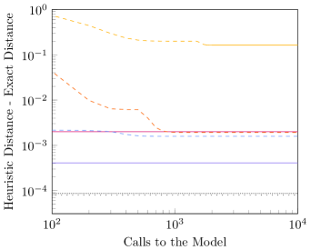
(d) CIFAR10 B Adversarial Fast-1k

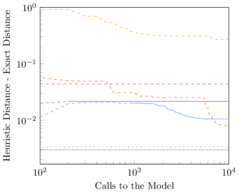
(e) MNIST B Adversarial Fast-10k

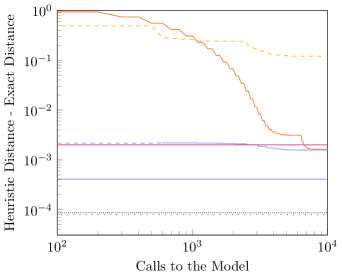
(f) CIFAR10 B Adversarial Fast-10k

Figure 19: Mean difference between the distance of the closest adversarial examples and the exact decision boundary distance for MNIST & CIFAR10 B Adversarial. A dashed line means that the attack found adversarial examples (of any distance) for only some inputs, while the absence of a line means that the attack did not find any adversarial examples. The loosely and densely dotted black lines respectively represent the balanced and strong attack pools. Both axes are logarithmic.

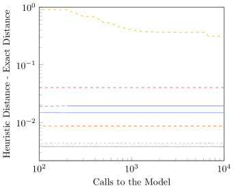
(a) MNIST B ReLU Fast-100

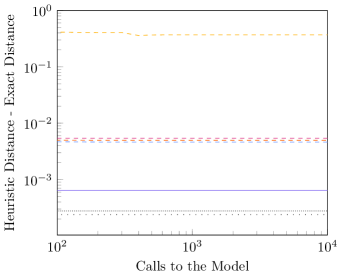
(b) CIFAR10 B ReLU Fast-100

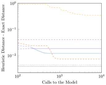
(c) MNIST B ReLU Fast-1k

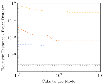
(d) CIFAR10 B ReLU Fast-1k

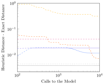
(e) MNIST B ReLU Fast-10k

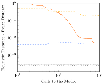
(f) CIFAR10 B ReLU Fast-10k

Figure 20: Mean difference between the distance of the closest adversarial examples and the exact decision boundary distance for MNIST & CIFAR10 B ReLU. A dashed line means that the attack found adversarial examples (of any distance) for only some inputs, while the absence of a line means that the attack did not find any adversarial examples. The loosely and densely dotted black lines respectively represent the balanced and strong attack pools. Both axes are logarithmic.

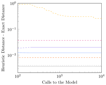
(a) MNIST C ReLU Fast-100

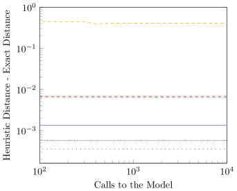
(b) CIFAR10 C ReLU Fast-100

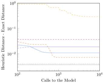
(c) MNIST C ReLU Fast-1k

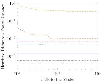
(d) CIFAR10 C ReLU Fast-1k

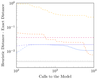
(e) MNIST C ReLU Fast-10k

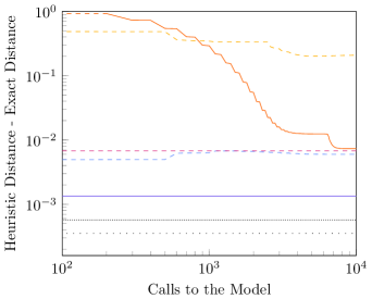
(f) CIFAR10 C ReLU Fast-10k

Figure 23: Mean difference between the distance of the closest adversarial examples and the exact decision boundary distance for MNIST & CIFAR10 C ReLU. A dashed line means that the attack found adversarial examples (of any distance) for only some inputs, while the absence of a line means that the attack did not find any adversarial examples. The loosely and densely dotted black lines respectively represent the balanced and strong attack pools. Both axes are logarithmic.

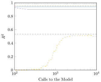
(a) MNIST C ReLU Fast-100

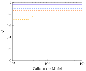
(b) CIFAR10 C ReLU Fast-100

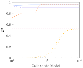
(c) MNIST C ReLU Fast-1k

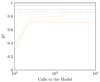
(d) CIFAR10 C ReLU Fast-1k

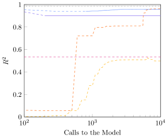
(e) MNIST C ReLU Fast-10k

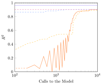
(f) CIFAR10 C ReLU Fast-10k

Figure 32: $R^{2}$ of linear model for the heuristic adversarial distances given the exact decision boundary distances for MNIST & CIFAR10 C ReLU. A dashed line means that the attack found adversarial examples (of any distance) for only some inputs, while the absence of a line means that the attack did not find any adversarial examples. The loosely and densely dotted black lines respectively represent the balanced and strong attack pools. The x axis is logarithmic.

References

- Athalye et al. (2018) Athalye, A., Carlini, N., and Wagner, D. Obfuscated gradients give a false sense of security: Circumventing defenses to adversarial examples. In International Conference on Machine Learning, pp. 274–283. PMLR, 2018.
- Awasthi et al. (2019) Awasthi, P., Dutta, A., and Vijayaraghavan, A. On robustness to adversarial examples and polynomial optimization. Advances in Neural Information Processing Systems, 32, 2019.
- Brendel et al. (2019) Brendel, W., Rauber, J., Kümmerer, M., Ustyuzhaninov, I., and Bethge, M. Accurate, reliable and fast robustness evaluation. Advances in Neural Information Processing Systems, 32, 2019.
- Brown et al. (2017) Brown, T. B., Mané, D., Roy, A., Abadi, M., and Gilmer, J. Adversarial patch. arXiv preprint arXiv:1712.09665, 2017.
- Bubeck et al. (2018) Bubeck, S., Lee, Y. T., Price, E., and Razenshteyn, I. Adversarial examples from cryptographic pseudo-random generators. arXiv preprint arXiv:1811.06418, 2018.
- Bubeck et al. (2019) Bubeck, S., Lee, Y. T., Price, E., and Razenshteyn, I. Adversarial examples from computational constraints. In International Conference on Machine Learning, pp. 831–840. PMLR, 2019.
- Carlini & Wagner (2016) Carlini, N. and Wagner, D. Defensive distillation is not robust to adversarial examples. arXiv preprint arXiv:1607.04311, 2016.
- Carlini & Wagner (2017a) Carlini, N. and Wagner, D. Adversarial examples are not easily detected: Bypassing ten detection methods. In Proceedings of the 10th ACM Workshop on Artificial Intelligence and Security, pp. 3–14, 2017a.
- Carlini & Wagner (2017b) Carlini, N. and Wagner, D. Magnet and ”Efficient defenses against adversarial attacks” are not robust to adversarial examples. arXiv preprint arXiv:1711.08478, 2017b.
- Carlini & Wagner (2017c) Carlini, N. and Wagner, D. Towards evaluating the robustness of neural networks. In 2017 IEEE Symposium on Security and Privacy (SP), pp. 39–57. IEEE, 2017c.
- Carlini et al. (2017) Carlini, N., Katz, G., Barrett, C., and Dill, D. L. Provably minimally-distorted adversarial examples. arXiv preprint arXiv:1709.10207, 2017.
- Chen et al. (2021) Chen, J., Guo, Y., Wu, X., Li, T., Lao, Q., Liang, Y., and Jha, S. Towards adversarial robustness via transductive learning. arXiv preprint arXiv:2106.08387, 2021.
- Croce et al. (2022) Croce, F., Gowal, S., Brunner, T., Shelhamer, E., Hein, M., and Cemgil, T. Evaluating the adversarial robustness of adaptive test-time defenses. arXiv preprint arXiv:2202.13711, 2022.
- Degwekar et al. (2019) Degwekar, A., Nakkiran, P., and Vaikuntanathan, V. Computational limitations in robust classification and win-win results. In Conference on Learning Theory, pp. 994–1028. PMLR, 2019.
- Ding et al. (2019) Ding, G. W., Wang, L., and Jin, X. AdverTorch v0.1: An adversarial robustness toolbox based on PyTorch. arXiv preprint arXiv:1902.07623, 2019.
- Dreossi et al. (2019) Dreossi, T., Ghosh, S., Sangiovanni-Vincentelli, A., and Seshia, S. A. A formalization of robustness for deep neural networks. arXiv preprint arXiv:1903.10033, 2019.
- Feinman et al. (2017) Feinman, R., Curtin, R. R., Shintre, S., and Gardner, A. B. Detecting adversarial samples from artifacts. arXiv preprint arXiv:1703.00410, 2017.
- Garg et al. (2020) Garg, S., Jha, S., Mahloujifar, S., and Mohammad, M. Adversarially robust learning could leverage computational hardness. In Algorithmic Learning Theory, pp. 364–385. PMLR, 2020.
- Gehr et al. (2018) Gehr, T., Mirman, M., Drachsler-Cohen, D., Tsankov, P., Chaudhuri, S., and Vechev, M. Ai2: Safety and robustness certification of neural networks with abstract interpretation. In 2018 IEEE symposium on security and privacy (SP), pp. 3–18. IEEE, 2018.
- Goodfellow et al. (2015) Goodfellow, I., Shlens, J., and Szegedy, C. Explaining and harnessing adversarial examples. In International Conference on Learning Representations, 2015. URL http://arxiv.org/abs/1412.6572.
- Gottlob et al. (2011) Gottlob, G., Greco, G., and Scarcello, F. Pure Nash equilibria: Hard and easy games. arXiv e-prints, pp. arXiv–1109, 2011.
- Grosse et al. (2017) Grosse, K., Manoharan, P., Papernot, N., Backes, M., and McDaniel, P. On the (statistical) detection of adversarial examples. arXiv preprint arXiv:1702.06280, 2017.
- Gurobi Optimization, LLC (2022) Gurobi Optimization, LLC. Gurobi Optimizer Reference Manual, 2022. URL https://www.gurobi.com.
- He et al. (2017) He, W., Wei, J., Chen, X., Carlini, N., and Song, D. Adversarial example defenses: ensembles of weak defenses are not strong. In Proceedings of the 11th USENIX Conference on Offensive Technologies, pp. 15–15, 2017.
- Hendrycks & Gimpel (2017) Hendrycks, D. and Gimpel, K. Early methods for detecting adversarial images. In International Conference on Learning Representations (Workshop Track), 2017.
- Hosseini et al. (2019) Hosseini, H., Kannan, S., and Poovendran, R. Are odds really odd? Bypassing statistical detection of adversarial examples. arXiv preprint arXiv:1907.12138, 2019.
- Katz et al. (2017) Katz, G., Barrett, C., Dill, D., Julian, K., and Kochenderfer, M. Reluplex: An efficient smt solver for verifying deep neural networks. arXiv preprint arXiv:1702.01135, 2017.
- Kingma & Ba (2014) Kingma, D. P. and Ba, J. Adam: A method for stochastic optimization. arXiv preprint arXiv:1412.6980, 2014.
- Koenker & Bassett Jr (1978) Koenker, R. and Bassett Jr, G. Regression quantiles. Econometrica: journal of the Econometric Society, pp. 33–50, 1978.
- Krizhevsky et al. (2009) Krizhevsky, A., Hinton, G., et al. Learning multiple layers of features from tiny images. Technical report, 2009.
- Kurakin et al. (2017) Kurakin, A., Goodfellow, I., and Bengio, S. Adversarial machine learning at scale. 2017.
- LeCun et al. (1998) LeCun, Y., Cortes, C., and J.C. Burges, C. The MNIST database of handwritten digits. http://yann.lecun.com/exdb/mnist/, 1998.
- Madry et al. (2018) Madry, A., Makelov, A., Schmidt, L., Tsipras, D., and Vladu, A. Towards deep learning models resistant to adversarial attacks. In International Conference on Learning Representations, 2018.
- Mahloujifar & Mahmoody (2019) Mahloujifar, S. and Mahmoody, M. Can adversarially robust learning leverage computational hardness? In Algorithmic Learning Theory, pp. 581–609. PMLR, 2019.
- Meng & Chen (2017) Meng, D. and Chen, H. MagNet: a two-pronged defense against adversarial examples. In Proceedings of the 2017 ACM SIGSAC Conference on Computer and Communications Security, pp. 135–147, 2017.
- Moosavi-Dezfooli et al. (2016) Moosavi-Dezfooli, S.-M., Fawzi, A., and Frossard, P. Deepfool: a simple and accurate method to fool deep neural networks. In Proceedings of the IEEE Conference on Computer Vision and Pattern Recognition, pp. 2574–2582, 2016.
- Papernot et al. (2016) Papernot, N., McDaniel, P., Wu, X., Jha, S., and Swami, A. Distillation as a defense to adversarial perturbations against deep neural networks. In 2016 IEEE Symposium on Security and Privacy (SP), pp. 582–597. IEEE, 2016.
- Papernot et al. (2017) Papernot, N., McDaniel, P., Goodfellow, I., Jha, S., Celik, Z. B., and Swami, A. Practical black-box attacks against machine learning. In Proceedings of the 2017 ACM on Asia Conference on Computer and Communications Security, pp. 506–519, 2017.
- Paszke et al. (2019) Paszke, A., Gross, S., Massa, F., Lerer, A., Bradbury, J., Chanan, G., Killeen, T., Lin, Z., Gimelshein, N., Antiga, L., Desmaison, A., Kopf, A., Yang, E., DeVito, Z., Raison, M., Tejani, A., Chilamkurthy, S., Steiner, B., Fang, L., Bai, J., and Chintala, S. PyTorch: An imperative style, high-performance deep learning library. In Wallach, H., Larochelle, H., Beygelzimer, A., d'Alché-Buc, F., Fox, E., and Garnett, R. (eds.), Advances in Neural Information Processing Systems 32, pp. 8024–8035. Curran Associates, Inc., 2019.
- Rauber et al. (2020) Rauber, J., Zimmermann, R., Bethge, M., and Brendel, W. Foolbox native: Fast adversarial attacks to benchmark the robustness of machine learning models in pytorch, tensorflow, and jax. Journal of Open Source Software, 5(53):2607, 2020.
- Roth et al. (2019) Roth, K., Kilcher, Y., and Hofmann, T. The odds are odd: A statistical test for detecting adversarial examples. In International Conference on Machine Learning, pp. 5498–5507. PMLR, 2019.
- Song et al. (2021) Song, M. J., Zadik, I., and Bruna, J. On the cryptographic hardness of learning single periodic neurons. Advances in neural information processing systems, 34:29602–29615, 2021.
- Stockmeyer (1976) Stockmeyer, L. J. The polynomial-time hierarchy. Theoretical Computer Science, 3(1):1–22, 1976.
- Tjeng et al. (2019) Tjeng, V., Xiao, K. Y., and Tedrake, R. Evaluating robustness of neural networks with mixed integer programming. In International Conference on Learning Representations, 2019.
- Tramer et al. (2020) Tramer, F., Carlini, N., Brendel, W., and Madry, A. On adaptive attacks to adversarial example defenses. Advances in Neural Information Processing Systems, 33:1633–1645, 2020.
- Weng et al. (2018) Weng, L., Zhang, H., Chen, H., Song, Z., Hsieh, C.-J., Daniel, L., Boning, D., and Dhillon, I. Towards fast computation of certified robustness for ReLU networks. In International Conference on Machine Learning, pp. 5276–5285. PMLR, 2018.
- Wu et al. (2020) Wu, Z., Lim, S.-N., Davis, L. S., and Goldstein, T. Making an invisibility cloak: Real world adversarial attacks on object detectors. In European Conference on Computer Vision, pp. 1–17. Springer, 2020.
- Xiao et al. (2019) Xiao, K. Y., Tjeng, V., Shafiullah, N. M., and Madry, A. Training for faster adversarial robustness verification via inducing ReLU stability. In International Conference on Learning Representations, 2019.