Charmonium production in high multiplicity pp collisions and the structure of the proton

Abstract

In this work we study charmonium production in high multiplicity proton-proton collisions. We investigate the role of the spatial distribution of partons in the protons and assume that the proton has a Y shape. In this configuration quarks are more at the surface and gluons in the inner part of the proton. Going from peripheral to more central and then to ultra-central proton-proton collisions, we go from quark-quark collisions to gluon-gluon collisions. Since gluons are much more abundant, the cross sections grow. In the case of charm production this growth is enhanced by the fact that, $\sigma(g+g\to c+\bar{c})>>\sigma(q+\bar{q}\to c+\bar{c})$. These effects can explain the growth seen in the data.

I Introduction

Surprising new features of proton proton collisions were revealed when the LHC collaborations became able to trigger on very high multiplicity events alice-psi7 ; alice-cc ; star18 ; alice19 ; alice20 ; alice-psi13 ; alice22 . In these events, the data presented evidence of collective behavior, which could be interpreted in terms of a hydrodynamical expansion of the system. However, to the best of our knowledge, so far no particle production model, hydrodynamic or non-hydrodynamic, matches all the features of the high-multiplicity pp data.

High multiplicity events come from ultracentral collisions, with very small impact parameter. In this regime we expect to observe several effects which can be responsible for the anomalous features of particle production, such as double parton scattering and parton saturation, caused by the larger saturation scale at lower impact parameters. Apart from these changes in the dynamics of the collisions, it is also possible that geometric effects associated with the spatial distribution of strongly interacting matter play a significant role.

Successfull models of the static proton are based on lattice QCD simulations, which show that quarks are bound by gluonic strings. This leads to the “Y” picture of the proton, where quarks are at the extremities tied by an Y-like gluon string, called gluon junction suga15 or baryon junction. This structure leads to a spatial configuration where the gluons are mostly in the center and the quark closer to the proton surface.

At first sight the static geometric configuration of the proton could be blurred or even completely washed out by a boost with the consequent parton evolution and branching. However, there are indications that the geometric organization of matter persists even at LHC energies. In manti23 it was shown that exclusive vector meson production is sensitive to the geometric deformation of the target. The authors conclude that the fluctuations in the nuclear geometry originating from the deformed structure are not washed out by the JIMWLK evolution and hence the deformations previously inferred from low-energy experiments will be visible in high-energy collisions. This suggests the the Y shape of the proton could survive the quantum evolution and manifest itself in high energy proton proton collisions.

The existence of the Y-shape configuration of the proton (along with its gluon junction) might shift the leading baryon distribution to smaller rapidities, providing an additional mechanism of baryon stopping. In these events the baryon number would be carried by the baryon junction, whereas in the traditional approach it is carried by the valence quarks (for a discussion see marb89 ). This interesting idea was proposed in khar96 , implemented in the Monte-Carlo event generator HIJING/B top04 and also in analytical models such as in bopp06 , being successfull in explaining the data on forward baryon production. The search for new effects of the baryon junction is in progress bran22 .

Having in mind what was said above, we would expect to see more manifestations of the proton Y shape. This was explored in  deb20 . One of the surprising aspects of high multiplicity proton proton collisions is the observation of the ridge effect and of elliptic flow. In Ref. deb20 a simple model based on the proton spatial configuration was developed to explain these phenomena. The authors improved the existing partonic Glauber model for proton-proton collisions loi16 , including anisotropic and inhomogeneous density profiles for the proton. They obtained a very good description of the $v_{2}$ measured by the ALICE collaboration in pp collisions at $\sqrt{s}=13$ TeV alice19 .

Another interesting observation made in high multiplicity events refers to charm production. In alice-cc the ALICE collaboration measured the $D^{0}$ yield as a function of the central rapidity density and found out an unexpectedly strong growth with the charged particle multiplicity. A similar trend was observed in the case of $J/\psi$ production. There are already some possible explanations of this growth of the charm yield given in Refs. cgc1 , boris20 , siddi20 and tripa22 .

In this work we will try to understand the data on charmonium production in high multiplicity events using the same geometrical model proposed in deb20 with the parameters fixed in that work. Charmonium production will be computed with the Color Evaporation Model (CEM). Leaving aside the quantitative aspects, the idea is fairly simple and it is as follows. The proton-proton collisions can be described by Y-Y collisions. Since we are not interested in the anisotropy aspects of the collision, we can take the average configuration of the Y over different orientations, i.e. we “rotate” the Y, obtaining a circular configuration with an inner gluonic shell and an outer quark shell. In other words, we have a core (gluon) - corona (quark) model of the proton. Going from peripheral to more central and then to ultra-central, we go from quark-quark collisions to gluon-gluon collisions. Since gluons are much more abundant, and since $\sigma(gg\to c\bar{c})\,>>\,\sigma(q\bar{q}\to c\bar{c})$ the cross sections grow strongly. These effects combined should explain the growth seen in the data.

In the next section we make some remarks concerning the proton structure, in Section III we review the version of the Glauber model adapted for proton-proton collisions and calculate the basic quantities, which are $N_{part}$ and $N_{coll}$. In Section IV we review the main formulas of the Color Evaporation Model used to study charm production. In Section V we show the results and compare them with data. Finally, some concluding remarks are presented in the last section.

II Remarks on the proton structure

In textbooks thomson (Chap. 7) we learn that in low energy elastic $e-p$ scattering we can determine the charge distribution of the proton. This is done by introducing electric, $G_{E}(Q^{2})$, and magnetic, $G_{M}(Q^{2})$, form factors and fitting the resulting (Rosenbluth) formula to the experimental data. Then, in a very specific limit, when $Q^{2}<<m^{2}_{p}$, we find that $Q^{2}\simeq\mathbf{q}^{2}$ and hence $G_{E}(Q^{2})\simeq G_{E}(\mathbf{q}^{2})$. In this limit the electric form factor can be interpreted as the Fourier transform of the charge distribution:

$$G_{E}(\mathbf{{q^{2}}})=\int\rho(\mathbf{r})e^{i\mathbf{q}\cdot\mathbf{r}}d^{3}\mathbf{r}$$ (1)

Hence, measuring $G_{E}(Q^{2})$ we find the $\rho$ shown in Fig. 1a. Moving away from the very low $Q^{2}$ limit, we do not have a well defined prescription to extract charge densities from the measured form factors (see, however, lorce for progress in this direction). From electron-proton high energy scattering in the high $Q^{2}$ limit, we know thomson (Chap. 8) that the incoming probe (photon or gluon) will indentify pointlike particles (partons) inside the proton, but we do not know how these partons are distributed in the transverse plane.

In the parton model description of deep inelastic scattering, the parton distribution functions depend on $Q^{2}$ and this dependence comes from the solution of the DGLAP evolution equations. In gla11 ; gla12 ; gla17 a different kind of evolution was proposed: the Renormalization Group Procedure for Effective Particles (REGPEP). In this approach, increasing the resolution scale we go from a configuration where the quarks are unresolved to a configuration with three effective quarks (quarks + antiquarks + gluons) disposed in the vertices of an equilateral triangle with a star-like juntion between them. Hence at high $Q^{2}$ the charge density tends to be moved from the origin, as shown qualitatively in Fig. 1b).

(a)		(b)

Figure 1: a) Charge distribution of the proton measured in elastic electron proton scattering at low energies and $Q^{2}\simeq 0$. b) Charge distribution suggested by the Y shape model of the proton.

The proton structure derived from the REGPEP approach was used to contruct a model successfully applied to describe several aspects of proton-proton collisions with high multiplicities kubi14 ; kubi15 ; gla16 and also inspired the model presented in deb20 and used here. In the next section we will discuss this model in more detail.

III The Glauber model for proton-proton collisions

In this section we briefly describe the model proposed in kubi15 ; kubi14 and successfully applied in deb20 . It combines the parton spatial distribution in the proton advanced in kubi15 ; kubi14 with the geometry machinery provided by the Glauber model glau07 . The quarks are anisotropically distributed, at the edges of the Y shape junction and the gluons are isotropically distributed arround the center kubi15 ; kubi14 .

Originally, the Glauber model was designed to represent the geometry of heavy-ions, including a dynamical component given by the nucleon cross sections. In loi16 it was adapted to proton-proton collisions. The effective number of partonic (subnucleonic) degrees of freedom was called $N_{c}$. The analysis of data performed in loi16 indicated that this number is $N_{c}\simeq 3-10$. Following loi16 and deb20 we will work with the effective number of partonic degrees of freedom (here we follow deb20 and call it $N_{g}$) and reinterpret $N_{part}$ and $N_{coll}$ as “number of partons that participate in the collision” and “number of binary collisions between partons” respectively.

In order to represent the proton internal structure, the matter distribution is given by kubi14 :

$$\rho_{p}(\mathbf{r};\mathbf{r}_{1},\mathbf{r}_{2},\mathbf{r}_{3})=\sum_{i=1}^{3}\rho_{q}(\mathbf{r}-\mathbf{r}_{i})+\rho_{g}\bigg{(}\mathbf{r}-\sum_{i=1}^{3}\frac{\mathbf{r}_{i}}{3}\bigg{)}$$ (2)

In this distribution, there are three effective quarks, called $i=1,2,3$, with the gaussian distribution:

$$\rho_{q}(r)=(1-\kappa)\frac{N_{g}}{3}\frac{e^{-r^{2}/2r_{q}^{2}}}{(2\pi)^{3/2}r_{q}^{3}}$$ (3)

and a gluon gaussian distribution:

$$\rho_{g}(r)=\kappa N_{g}\frac{e^{-r^{2}/2r_{g}^{2}}}{(2\pi)^{3/2}r_{g}^{3}}$$ (4)

centered at the average coordinate of the quarks. In these distributions, $N_{g}$ is the total number of partons in the proton, $\kappa$ is the fraction of $N_{g}$ that corresponds to the gluon body, $r_{q}$ is the radius of the effective quark and $r_{g}$ the radius of the gluon body. These parameters are fixed and we take them from previous works with this model. In Fig. 2 we show the contour plot of these distributions. Fig. 3 shows a projection of these distributions and it represents what we would see moving (up and to the right) from the center of the proton to the peak of the quark density (in Fig. 2a) plotted together with the gluon density from Fig. 2b. It is an illustration of the “core-corona” aspect of the model and helps to understand the results.

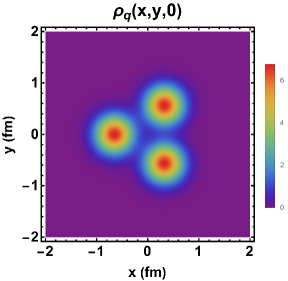
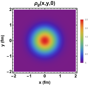
(a)		(b)

Figure 2: a) Quark and b) gluon distributions in the transverse plane.

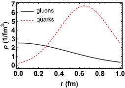
Figure 3: Quark and gluon distributions. Projection of Fig. 2 along a diagonal direction, starting from the center of the proton and passing through one maximum of the quark density.

With the quark and gluon densities we can calculate the inputs to be used in the Glauber model. The proton thickness, $T_{p}(x,y)$, is given by:

$$T_{p}(x,y)=\int\rho_{p}(x,y,z)dz=T_{p}^{q}(x,y)+T_{p}^{g}(x,y)$$ (5)

where $T_{p}^{q}(x,y)$ and $T_{p}^{g}(x,y)$ come from the quark and gluon terms of Eq.(2) and are given by:

$$T_{p}^{q}(x,y)=\frac{N_{g}(1-\kappa)}{6\pi r_{q}^{2}}\sum_{i=1}^{3}e^{-\frac{(x-x_{i})^{2}+(y-y_{i})^{2}}{2r_{q}^{2}}}$$ (6)

and

$$T_{p}^{g}(x,y)=\frac{N_{g}\kappa}{2\pi r_{g}^{2}}e^{-\frac{(x-\sum_{i=1}^{3}x_{i}/3)^{2}+(y-\sum_{i=1}^{3}y_{i}/3)^{2}}{2rg^{2}}}$$ (7)

The overlap function can be calculated as:

$$T_{pp\prime}(b)=\int T_{p}(x-b/2,y)T_{p\prime}(x+b/2,y)dxdy$$ (8)

The above equation can be split into four terms. Because of the gaussian forms involved, all the integrals can be done analytically. The quark-quark term is given by:

$$T_{pp\prime}^{qq}(b)=\int T_{p}^{q}(x-b/2,y)T_{p\prime}^{q}(x+b/2,y)dxdy=\frac{N_{g}^{2}(1-\kappa)}{36\pi r_{q}^{2}}\sum_{i=1}^{3}\sum_{j=1}^{3}\exp\bigg{(}-\frac{\big{(}b+(x_{i}-x_{j})\big{)}^{2}+\big{(}y_{i}-y_{j}\big{)}^{2}}{4rq^{2}}\bigg{)}$$ (9)

with the quarks $i=1,2,3$ from the proton $p$, and $j=1,2,3$ from the proton $p\prime$. The gluon-gluon term can be calculated as:

$$T_{pp\prime}^{gg}(b) = \int T_{p}^{g}(x-b/2,y)T_{p\prime}^{g}(x+b/2,y)dxdy$$ (10)

$$= \frac{N_{g}^{2}\kappa^{2}}{4\pi r_{g}^{2}}\exp\bigg{(}-\frac{\big{(}b+\sum_{i=1}^{3}x_{i}/3-\sum_{j=1}^{3}x_{j}/3\big{)}^{2}+\big{(}\sum_{i=1}^{3}y_{i}/3-\sum_{j=1}^{3}y_{j}/3\big{)}^{2}}{4rg^{2}}\bigg{)}$$

The gluon-quark term, which accounts for the interactions between the gluons from $p$ with quarks from $p\prime$, is given by:

$$T_{pp\prime}^{gq}(b) = \int T_{p}^{g}(x-b/2,y)T_{p\prime}^{q}(x+b/2,y)dxdy$$ (11)

$$= \frac{N_{g}^{2}\kappa(1-\kappa)}{6\pi(r_{q}^{2}+r_{g}^{2})}\sum_{j=1}^{3}\exp\bigg{(}-\frac{\big{(}b+\sum_{i=1}^{3}x_{i}/3-x_{j}\big{)}^{2}+\big{(}\sum_{i=1}^{3}y_{i}/3-y_{j}\big{)}^{2}}{2(r_{q}^{2}+r_{g}^{2})}\bigg{)}$$

The last term refers to the interaction between the quarks from $p$ and the gluons from $p\prime$. It is given by:

$$T_{pp\prime}^{qg}(b) = \int T_{p}^{q}(x-b/2,y)T_{p\prime}^{g}(x+b/2,y)dxdy$$ (12)

$$= \frac{N_{g}^{2}\kappa(1-\kappa)}{6\pi(r_{q}^{2}+r_{g}^{2})}\sum_{i=1}^{3}\exp\bigg{(}-\frac{\big{(}b+x_{i}-\sum_{j=1}^{3}x_{j}/3\big{)}^{2}+\big{(}y_{i}-\sum_{j=1}^{3}y_{j}/3\big{)}^{2}}{2(r_{q}^{2}+r_{g}^{2})}\bigg{)}$$

The total thickness function of the model is obtained by inserting Eqs. (9), (10), (11) and (12) into Eq.(8). It reads:

$$T_{pp\prime}(b)=T_{pp\prime}^{qq}(b)+T_{pp\prime}^{gg}(b)+T_{pp\prime}^{gq}(b)+T_{pp\prime}^{qg}(b)$$ (13)

The number of binary collisions is then given by:

$$N_{coll}=T_{pp\prime}(b)\sigma^{pp}$$ (14)

where $\sigma^{pp}$ is the parton-parton cross section, which is a parameter often used in the literature. The obtained values in the wounded quark model of Ref. sigpp1 , in the hydrodynmical analysis of Ref. sigpp2 and in the parton transport model of Ref. sigpp3 are all in the range $\sigma^{pp}=5-10$ mb. The number of participants is calculated according to

$$N_{part}(b)=N_{coll}^{x}(b)$$ (15)

where $x=0.75$ glau07 . In the above equations, $N_{part}$ and $N_{coll}$ are calculated for a given quark configuration, i.e. a given choice of the quark coordinates in the projectile proton $\mathbf{r}_{i}=(x_{i},y_{i})$ and in the target proton $\mathbf{r^{\prime}}_{i}=({x^{\prime}}_{i},{y^{\prime}}_{i})$. In order to simulate a proton-proton collision we must now take the average over these configurations. This is best done writting the quark position in polar coordinates:

$$\mathbf{r}_{i}=\frac{d}{2}\big{(}\cos(\phi_{i}+\alpha),\sin(\phi_{i}+\alpha)\big{)}\,\,\,\,\,\,\,\,\,\,\,\,\,\mbox{and}\,\,\,\,\,\,\,\,\,\,\,\,\,\mathbf{r^{\prime}}_{i}=\frac{d}{2}\big{(}\cos(\phi_{i}+\beta),\sin(\phi_{i}+\beta)\big{)}$$ (16)

where $\phi_{1}=\pi/3$, $\phi_{2}=-\pi/3$ and $\phi_{3}=-\pi$. This choice of positions generates protons in which the quarks are in the vertices of equilateral triangles in the $x-y$ plane, rotated by the angles $\alpha$ and $\beta$ ($\alpha\text{, }\beta\in[0,2\pi]$) around the $z$ axis. The angles are randomly chosen. For $d=1.3\text{ fm}$, one example of initial condition is shown in Fig. 4a.

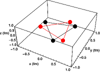
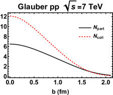
(a)		(b)

Figure 4: a) Example of initial spatial configuration of the two colliding protons. b) Average of $N_{part}$ and $N_{coll}$ over different quark spatial configurations for each impact parameter.

Using the parameters of Table 1 and fixing the impact parameter we choose the angles $\alpha$ and $\beta$. With them we calculate the coordinates $\mathbf{r}_{i}$ and then the thickness function, which we substitute into Eqs. (14) and (15) obtaining $N_{coll}$ and $N_{part}$. We repeat this procedure for 10000 choices and take the average. After that, we move to the next impact parameter and repeat the steps. In the end we obtain $N_{coll}$ and $N_{part}$ as a function of the impact parameter. The results for $pp$ collisions at $\sqrt{s}=7\text{ TeV}$ are shown in Fig.  4b. Here the impact parameter is such that $b\in[0,2.2]\text{ fm}$, with steps $\Delta b=0.1\text{ fm}$. The same procedure was repeated for $\sqrt{s}=13\text{ TeV}$. The resulting curves are quite similar to those shown in Fig.  4b but with higher maximum values. For conciseness we do not show them here.

Table 1: Input used in the parton densities and in the Glauber model. See text for definitions.

$N_{g}$ deb20	$10$
$\kappa$ deb20	$0.5$
$r_{q}\text{ (fm)}$deb20	$0.25$
$r_{g}\text{ (fm)}$ kubi14	$0.5$
$\sigma^{pp}\text{ (mb)}$ ($\sqrt{s}=7$ TeV) sigpp1 ; sigpp2	$4.3$
$\sigma^{pp}\text{ (mb)}$ ($\sqrt{s}=13$ TeV) sigpp1 ; sigpp2	$7.6$
$d\text{ (fm)}$ deb20	1.3
$x$ glau07	0.75

IV Charmonium production

Charm production can be described by perturbative QCD and there are currently several calculations which reproduce the data with very good accuracy. For our purposes a leading order calculation is sufficient. Therefore we shall employ the Color Evaporation Model vogt18 ; vogt07 (CEM). This model provides a way to calculate the production of charm pairs through the processes $gg\rightarrow c\bar{c}$ and $q\bar{q}\rightarrow c\bar{c}$. The cross section for $J/\psi$ production is then given simply by:

$$\sigma^{CEM} = \mathbf{F}K\sum_{i,j}\int_{(2m_{c})^{2}}^{(\Lambda)^{2}}dm^{2}\int dx_{1}dx_{2}f_{i}(x_{1},\mu^{2})f_{j}(x_{2},\mu^{2})\sigma_{ij}(m^{2})\delta(m^{2}-x_{1}x_{2}s)$$ (17)

$$= \sigma_{gg}^{CEM}+\sigma_{q\bar{q}}^{CEM}$$

where $f(x,\mu^{2})$ are the parton distribution functions at the renormalization scale $\mu$ and $\Lambda$ is a cut-off. In the case of open charm production $\Lambda=\sqrt{s}$ and for $J/\psi$ production $\Lambda=2\,m_{D}$. The parameter $F$ is equal to the percentage of the $c\bar{c}$ states with $2\,m_{c}<m<2\,m_{D}$ which becomes a $J/\psi$. We will assume that $m_{c}=1200\text{ MeV}$ and $m_{D}=1800\text{ MeV}$. The symbol $\sigma_{ii}(m^{2})$ represents the elementary $gg\rightarrow c\bar{c}$ and $q\bar{q}\rightarrow c\bar{c}$ cross sections. At leading order, they are given by:

$$\sigma_{gg}(m^{2})=\frac{\pi\alpha_{s}^{2}(m^{2})}{3m^{2}}\bigg{\{}\big{(}1+\frac{4m_{c}^{2}}{m^{2}}+\frac{m_{c}^{4}}{m^{4}}\big{)}\ln\bigg{(}\frac{1+\lambda}{1-\lambda}\bigg{)}-\frac{1}{4}\big{(}7+\frac{31m_{c}^{2}}{m^{2}}\big{)}\lambda\bigg{\}}$$ (18)

and

$$\sigma_{q\bar{q}}(m^{2})=\frac{8\pi\alpha_{s}^{2}(m^{2})}{27m^{2}}\bigg{(}1+\frac{2m_{c}^{2}}{m^{2}}\bigg{)}\lambda$$ (19)

where $\alpha_{s}$ (the strong coupling constant) and $\lambda$ are given by:

$$\alpha_{s}(\mu^{2})=\frac{12\pi}{(33-2N_{f})\ln\big{(}\frac{\mu^{2}}{\Lambda_{QCD}^{2}}\big{)}}\,\,\,\,\,\,\,\,\,\,\,\,\,\,\,\,\,\,\,\,\,\,\,\,\,\,\,\,\,\,\,\,\,\,\,\,\,\,\lambda=\bigg{(}1-\frac{(2m_{c})^{2}}{m^{2}}\bigg{)}^{1/2}$$ (20)

where $N_{f}$ is the number of flavors and $\Lambda_{QCD}=200\text{ MeV}$. The parameter $K$ is introduced to account for higher order corrections. We can fix it setting $F=1$, $\Lambda=\sqrt{s}$ and adjusting the cross section Eq. (17) to the experimental data on open charm production phenix02 ; phenix06 ; alice12 . The result is shown in Fig. 5. We obtain a good fit of these data with $K=2$. Imposing that $\lambda$ is real leads to the kinematical constraint $x_{1}x_{2}s\geq 4m_{c}^{2}$. Since the smallest value of $x_{1}$ occurs for $x_{2}=1$, the parton momentum fraction must be such that $(2m_{c})^{2}/s\leq x_{1}\leq 1$ and $(2m_{c})^{2}/(sx_{1})\leq x_{2}\leq 1$. The parton distribution functions, used with $Q^{2}=2.4^{2}\text{ GeV}^{2}$, are taken from the CTEQ5 set PDFs . Finally, the number of $c\bar{c}$ pairs is given by:

$$N_{c\bar{c}}(b)=T_{pp\prime}^{gg}(b)\,\sigma_{gg}^{CEM}+T_{pp\prime}^{qq}(b)\,\sigma_{qq}^{CEM}$$ (21)

The $T_{pp\prime}^{qg}(b)$ and $T_{pp\prime}^{gq}(b)$ terms of Eq.(13) are not included because the quark-gluon interactions do not produce $c\bar{c}$ pairs.

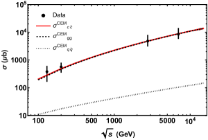
Figure 5: Charm production cross sections. Contribution of $gg\rightarrow c\bar{c}$ (dashed line), $q\bar{q}\rightarrow c\bar{c}$ (dotted line) and total cross-section (solid line). The experimental data are from phenix02 ; phenix06 ; alice12 .

V Results

We now address the experimental data of alice-psi7 ; alice-psi13 ; alice-cc . Following the experimental papers, we present the yields in terms of the normalized pseudo-rapidity and rapidity densities:

$$\frac{({dN}/{d\eta}(\eta=0))}{\langle{dN}/{d\eta}\rangle}\,\,\,\,\,\,\,\,\,\,\,\,\,\,\,\,\,\,\,\,\,\,\,\,\,\,\,\,\,\,\,\,\,\,\,\,\frac{({dN}/{dy}(y=0))}{\langle{dN}/{dy}\rangle}$$ (22)

The charged particle pseudorapidity density at $\eta=0$ is calculated as in kn01 :

$$\frac{dN}{d\eta}(\eta=0)=n_{pp}(s)\big{\{}(1-f)\frac{N_{part}}{2}+fN_{coll}\big{\}}$$ (23)

where $N_{part}$ and $N_{coll}$ are given by (15) and (14) respectively and $n_{pp}(s)$ is given by kn01 :

$$n_{pp}(s)=2.5-0.25\log[s]+0.023(\log[s])^{2}$$ (24)

The factor $f$ is the fraction of hard processes in the collision and can be estimated through the ratio: $f=\sigma_{minijet}/\sigma_{inel}$ as in mini1 ; mini2 . A minijet is defined as the result of a parton-parton collision with $p_{T}>p_{T0}$ with $p_{T0}$ being of the order of a few GeV (with a possible dependence on $\sqrt{s}$). The average density $\langle dN/d\eta\rangle$ is a number given by each experimental group and we show them in Table II, together with the $F$ parameter.

Table 2: Input used for $J/\psi$ production. See text for definitions.

	$\sqrt{s}=7$ TeV	$\sqrt{s}=13$ TeV
f	19 % mini1 ; mini2	16 % mini1 ; mini2
F	1.5 % vogt18 ; vogt07	4.3 % vogt18 ; vogt07
$\langle dN/d\eta\rangle$	$6.1$ alice-dn-13	$6.4$ alice-dn-13
$\langle dN_{J/\psi}/dy\rangle$	$8.2\times 10^{-5}$ alice-psi7	$7.9\times 10^{-5}$ alice-psi13

The $J/\psi$ rapidity density, $dN_{J/\psi}/dy$, is obtained from the differential form of Eq.(21):

$$\frac{dN_{c\bar{c}}}{dy}(b)=T_{pp\prime}^{gg}(b)\,\frac{d\sigma_{gg}^{CEM}}{dy}+T_{pp\prime}^{qq}(b)\,\frac{d\sigma_{qq}^{CEM}}{dy}$$ (25)

We can evaluate this expression starting from Eq.(17) and applying the following change of variables:

$$x_{1}=\frac{p_{T}}{\sqrt{s}}e^{y}\,\,\,\,\,\,\,\,\,\,\,\,x_{2}=\frac{p_{T}}{\sqrt{s}}e^{-y}\,\,\,\,\,\,\,\,\,\,\,\,x_{1}x_{2}s=p_{T}^{2}\,\,\,\,\,\,\,\,\,\,\,\,dx_{1}dx_{2}\rightarrow\frac{2p_{T}}{s}dydp_{T}$$ (26)

After changing the variables from $(x_{1},x_{2})$ to $(y,p_{T})$, we integrate over $p_{T}$, differentiate with respect to $y$ and take $y=0$. The results for the $J/\psi$ yields for $\sqrt{s}=7\text{ TeV}$ and $\sqrt{s}=13\text{ TeV}$ are shown in Fig. 6. As it can be seen we obtain a very good description of data. One might argue that we have too many input parameters and this reduces the predictive power of the model. However, all these input numbers are strongly constrained by other independent studies of other observables. As we notice in the tables, all the numbers are consistent with the equivalent numbers found elesewhere. We took the precaution of nowhere using exotic values for any of these numbers. In view of the results, we conclude that the $J/\psi$ dependence on the charged multiplicity is compatible with the geometrical picture of the proton used here. The analysis can be extended to $D$ production, to beauty production and to different cuts in $p_{T}$ and rapidity. We are already working in these topics.

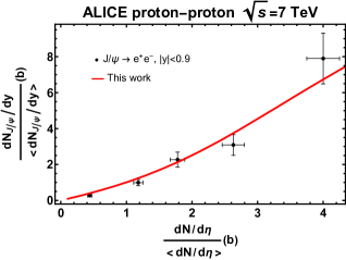
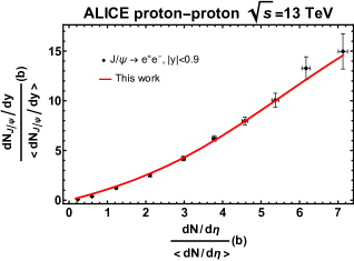
(a)		(b)

Figure 6: a) $J/\psi$ relative yield in $pp$ collisions at $\sqrt{s}_{NN}=7\text{ TeV}$. The experimental data are from alice-psi7 . b) $J/\psi$ relative yield in $pp$ collisions at $\sqrt{s}_{NN}=13\text{ TeV}$. The experimental data are from alice-psi13 .

VI Concluding remarks

We have developed the idea that proton-proton collisions can be described by Y-Y collisions. Averaging over orientations this yields a circular configuration with an inner gluonic shell and an outer quark shell. This is a core (gluon) - corona (quark) model of the proton. Going from peripheral to more central and then to ultra-central, we go from quark-quark collisions to gluon-gluon collisions. Since gluons are much more abundant, and since $\sigma(gg\to c\bar{c})\,>>\,\sigma(q\bar{q}\to c\bar{c})$ the cross sections grow strongly. These effects combined explain the growth seen in the data.

This behavior was qualitatively expected and we have used a combination of models to implement this idea quantitatively: a model for the parton spatial densities deb20 ; the Glauber model for proton-proton collisions loi16 and the color evaporation model for charmonium production vogt18 ; vogt07 . These models had been previously tested in other contexts and were shown to give good results. All the parameters used were strongly constrained by the analysis of other data and here we had little room to change them. We obtained a good description of charmonium production in proton-proton events with high multiplicities. This encourages us to further extend this model to open charm production and to proton-nucleus collisions.

- (1) B. Abelev et al. [ALICE], Phys. Lett. B 712, 165 (2012).
- (2) J. Adam et al. [ALICE Collaboration], JHEP 09, 148 (2015).
- (3) J. Adam et al. [STAR], Phys. Lett. B 786, 87 (2018).
- (4) K. Gajodsov, [ALICE Collaboration], Nucl. Phys. A 982, 487 (2019).
- (5) S. Acharya et al. [ALICE], Eur. Phys. J. C 80, 167 (2020).
- (6) S. Acharya et al. [ALICE], Phys. Lett. B 810, 135758 (2020).
- (7) S. Acharya et al. [ALICE], JHEP 06, 015 (2022).
- (8) N. Sakumichi and H. Suganuma, Phys. Rev. D 92, 034511 (2015).
- (9) H. Mantysaari, B. Schenke, C. Shen and W. Zhao, arXiv:2303.04866.
- (10) G. N. Fowler, F. S. Navarra, M. Plumer, A. Vourdas, R. M. Weiner and G. Wilk, Phys. Rev. C 40, 1219 (1989).
- (11) D. Kharzeev, Phys. Lett. B 378, 238 (1996),
- (12) V. Topor Pop, M. Gyulassy, J. Barrette, C. Gale, X. N. Wang and N. Xu, Phys. Rev. C 70, 064906 (2004).
- (13) F. W. Bopp and M. Shabelski, Eur. Phys. J. A 28, 237 (2006).
- (14) J. D. Brandenburg, N. Lewis, P. Tribedy and Z. Xu, [arXiv:2205.05685 [hep-ph]].
- (15) S. Deb, G. Sarwar, D. Thakur, P. Subramani, R. Sahoo and J. e. Alam, Phys. Rev. D 101, 014004 (2020).
- (16) C. Loizides, Phys. Rev. C 94, 024914 (2016).
- (17) Y.-Q. Ma, P. Tribedy, R. Venugopalan and K. Watanabe Phys. Rev. D 98, 074025 (2018).
- (18) B. Z. Kopeliovich, H. J. Pirner, I. K. Potashnikova, K. Reygers and I. Schmidt, Phys. Rev. D 101, 054023 (2020).
- (19) E. Levin, I. Schmidt and M. Siddikov, Eur. Phys. J. C 80, 560 (2020).
- (20) T. Tripathy et al., arXiv:2209.08784.
- (21) M. Thomson, “Modern Particle Physics”, Cambridge University Press, (2013).
- (22) C. Lorcé, Phys. Rev. Lett. 125, 232002 (2020).
- (23) S. Glazek, Few-Body Syst. 52, 367, (2012).
- (24) S. D. Glazek, Phys. Rev. D 85, 125018 (2012).
- (25) S. D. Głazek and A. P. Trawiński, Few Body Syst. 58, 49 (2017).
- (26) P. Kubiczek, “Geometrical model of azimuthal correlations in high-multiplicity proton-proton collisions”, Thesis, University of Warsaw, (2014).
- (27) P. Kubiczek and S. D. Głazek, Lith. J. Phys. 55, 155 (2015).
- (28) S. D. Glazek and P. Kubiczek, Few Body Syst. 57, 425 (2016).
- (29) M.L. Miller et al., Annu. Rev. Nucl. Part. Sci. 57, 205 (2007).
- (30) P. Bożek, W. Broniowski, M. Rybczyński, Phys. Rev. C 94, 014902 (2016).
- (31) H. Drescher, A. Dumitru, C. Gombeaud, J. Ollitraut, Phys. Rev. C 76, 024905 (2007).
- (32) Z. Xu and C. Greiner, Nucl. Phys. A 774, 787 (2006)
- (33) V. Cheung and R. Vogt, Phys. Rev. D 98, 114029 (2018);
- (34) R. Vogt, “Ultrarelativistic heavy-ion collisions”, Elsevier, (2007).
- (35) K. Adcox et al. [PHENIX Collaboration], Phys. Rev. Lett. 88, 192303 (2002).
- (36) A. Adare et al. [PHENIX Collaboration], Phys. Rev. Lett. 97, 252002 (2006).
- (37) B. Abelev et al. [ALICE Collaboration], JHEP 1207, 191 (2012).
- (38) H.L. Lai et al. [CTEQ Collaboration], Eur. Phys. J. C 12, 375 (2000).
- (39) D. Kharzeev, M. Nardi, Phys. Lett. B 507, 121 (2001).
- (40) P. Kotko, A. M. Stasto and M. Strikman, Phys. Rev. D 95, 054009 (2017).
- (41) I. Sarcevic, S. D. Ellis and P. Carruthers, Phys. Rev. D 40, 1446 (1989).
- (42) J. Adam et al. [ALICE Collaboration], Phys. Lett. B 753, 319 (2016).