Efficient Contextformer: Spatio-Channel Window Attention for Fast Context Modeling in Learned Image Compression

Abstract

In this work, we introduce Efficient Contextformer (eContextformer) for context modeling in lossy learned image compression, which is built upon our previous work, Contextformer. The eContextformer combines the recent advancements in efficient transformers and fast context models with the spatio-channel attention mechanism. The proposed model enables content-adaptive exploitation of the spatial and channel-wise latent dependencies for a high performance and efficient entropy modeling. By incorporating several innovations, the eContextformer features improved decoding speed, model complexity and rate-distortion performance over previous work. For instance, compared to Contextformer, the eContextformer requires 145x less model complexity, 210x less decoding speed and achieves higher average bit savings on the Kodak, CLIC2020 and Tecnick datasets. Compared to the standard Versatile Video Coding (VVC) Test Model (VTM) 16.2, the proposed model provides up to 17.1% bitrate savings and surpasses various learning-based models.

I Introduction

Online media consumption generates an ever-growing demand for higher-quality and lower-bitrate content [1, 2]. This demand drives advancements in both classical and learned image compression (LIC) algorithms. The early LIC algorithms [3, 4, 5, 6, 7, 8, 9, 10, 11, 12, 13, 14, 15, 16, 17] provide competitive rate-distortion performance to classical standards such as JPEG [18], JPEG2000 [19] and BPG [20] (HEVC [21] Intra mode), and the recent LIC proposals [22, 23, 24] already outperform state-of-the-art video coding standards such as VVC [25].

The best performing LIC frameworks [3, 4, 5, 6, 7, 8, 9, 10, 11, 12, 13, 14, 15, 16, 17, 23, 22, 24] use an autoencoder which applies a non-linear, energy compacting transform [26] to an input image. Such frameworks learn a so-called forward–backward adaptive entropy model in order to create a low-entropy latent space representation of the image. The model estimates the probability distribution by conditioning the distribution to two types of information – one is a signalled prior (a.k.a. forward adaptation [4]), and the other is implicit contextual information extracted by an autoregressive context model (a.k.a. backward adaptation [5]). The performance of the backward adaptation is a major factor for the efficiency of the LIC framework, and methods to improve its performance have been actively investigated. Various context model architectures have been proposed – e.g. 2D masked convolutions using local dependencies [5, 11, 9, 6, 8, 7]; channel-wise autoregressive mechanisms exploiting channel dependencies [10, 16, 24]; non-local simplified attention-based models capturing long-range spatial dependencies [23, 12]; sophisticated transformer-based models leveraging a great degree of content-adaptive context modeling [17, 24].

Using an autoregressive model requires recursive access to previously processed data, which results in slow decoding time and inefficient utilization of NPU/GPU. To remedy this, some researchers [13, 11, 24] optimized the decoding process by using wavefront parallel processing (WPP) similar to the one used in classical codecs [27]. The WPP significantly increases parallelism, but still requires a large number of autoregressive steps for the processing of large images. A more efficient approach is to split the latent elements into groups and code each group separately [14, 15, 16, 17, 22]. The latent elements might be split into e.g. spatial patches [14], channel segments [16], or using a checkered pattern [15]. The researchers also investigated a combination of the channel-wise and the checkered grouping [22]. Such parallelization approaches can reduce decoding time by 2-3 orders of magnitude, at the cost of higher model complexity and up to 3% performance drop. For instance, the patch-wise model [14] uses a recurrent neural network to share information between patches. Other works [16, 22] use channel-wise model and implement additional convolutional layers to combine decoded channel segments.

Our previous work [24] proposed the Contextformer utilizing spatio-channel attention, which outperformed contemporary LIC frameworks [3, 4, 5, 6, 7, 8, 9, 10, 11, 12, 16, 17, 23]. However, the decoding time and model complexity of Contextformer make it unsuitable for real-time operation. In this work, we propose a fast and low-complexity version of the Contextformer, which we call Efficient Contextformer (eContextformer). We extend the window attention of [28] to spatio-channel window attention in order to achieve a high performance and low complexity context model. Additionally, we use the checkered grouping to increase parallelization and reduce autoregressive steps in context modeling. By exploiting the properties of eContextformer, we also propose algorithmic optimizations to reduce complexity and runtime even further.

In terms of PSNR, our model outperforms VTM 16.2 [29] on Kodak [30], CLIC2020 [31] (Professional and Mobile) and Tecnick [32] datasets, providing average bitrate savings of 10.9%, 12.4%, 6.9% and 12.6%, respectively. Our optimized implementation requires 145x less multiply-accumulate (MAC) operations and takes 210x less decoding time compared to the earlier Contextformer. It also contains significantly less model parameters compared to other channel-wise autoregressive and transformer-based prior-art context models [16, 17]. Furthermore, due to its manageable complexity, eContextformer can be used with an online rate-distortion optimization (oRDO) similar to the one in [33]. With oRDO enabled, the performance of our model reaches up to 17.1% average bitrate saving in terms of PSNR over VTM 16.2 [29].

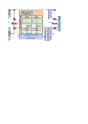
(a)

(b)

(c)

(d)

(e)

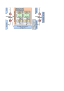
(f)

Figure 1: Illustration of the context modeling process, where the symbol probability of the current latent variable $\left(\leavevmode\hbox to7.06pt{\vbox to7.06pt{\text{[drawing]}}}\right)$ estimated by aggregating the information of the latent variables $\left(\leavevmode\hbox to7.06pt{\vbox to7.06pt{\text{[drawing]}}}\right)$. The previously decoded latent elements not joining to context modeling and yet to be coded elements are depicted as $\left(\leavevmode\hbox to7.06pt{\vbox to7.06pt{\text{[drawing]}}}\right)$ and $\left(\leavevmode\hbox to7.06pt{\vbox to7.06pt{\text{[drawing]}}}\right)$, respectively. The illustrated context models are (a) the model with 2D masked convolutions [5, 11], (b) the model with 3D masked convolutions [6, 10], (c) channel-wise autoregressive model [16], (d) simple attention-based model [23], and (e–f) Contextformer with sfo and cfo coding mode [24], respectively.

II Related Work

II-A Transformers in Computer Vision

The underlying principle of the transformer network [34] can be summarized as a learned projection of sequential vector embeddings $\bm{x}\in\mathbb{R}^{S\times d_{e}}$ into sub-representations of query $\bm{Q}\in\mathbb{R}^{S\times d_{e}}$, key $\bm{K}\in\mathbb{R}^{S\times d_{e}}$ and value $\bm{V}\in\mathbb{R}^{S\times d_{e}}$, where $S$ and $d_{e}$ denote the sequence length and the embedding size, respectively. Subsequently, a scaled dot-product calculates the attention, which weighs the interaction between the query and key-value pairs. The $\bm{Q}$, $\bm{K}$ and $\bm{V}$ are split into $h$ groups, known as heads, which enables parallel computation and greater attention granularity. The separate attention of each head is finally combined by a learned projection $W$. After the attention module, a point-wise multi-layer perceptron (MLP) is independently applied to all positions in $S$, in order to provide non-linearity. For autoregressive tasks, masking of the attention is required to ensure the causality of the interactions within the input sequence. The multi-head attention with masking can be described as:

$$Attn(\bm{Q},\bm{K},\bm{V})=\text{concat}({head}_{1},\ldots,{head}_{h})\bm{W},$$ (1a)

$$head_{i}(\bm{Q}_{i},\bm{K}_{i},\bm{V}_{i})=\text{softmax}\left(\frac{\bm{Q}_{i}\bm{K}_{i}^{T}}{d_{k}}\odot\bm{M}\right)\bm{V}_{i},$$ (1b)

where the mask $\bm{M}\in\mathbb{R}^{S\times S}$ contains weights of $-\infty$ in the positions corresponding to interactions with elements which are not processed yet, and ones for the rest. The operator $\odot$ denotes the Hadamard product.

The vanilla implementation of a convolutional neural network (CNN) [35] exploits the local correlations with static weights after training. The attention mechanism inherent to transformers uses content-adaptive weighting, which captures long-distance relations [36]. Such property makes transformers potentially more suitable for various computer vision (CV) tasks [37, 38, 39, 40]. As computational complexity of a vanilla transformer grows quadratically with the length of the sequence $S$, those are hardly applicable for high-resolution images. As one potential solution, Dosovitskiy et al. [38] proposed the Vision Transformer (ViT). The ViT decomposes large images into non-overlapping 2D patches and computes a global attention between the flattened patches. The ViT outperforms its CNN-based counterparts, but it has a trade-off between the patch size and its complexity – the tasks depending on pixel-level decisions, such as image segmentation, require smaller patch sizes, while the complexity remains quadratic in the number of patches. As an alternative to global attention, [41, 40, 24] propose to use sliding window attention to limit the attention span. The attention computation within a window has relatively lower complexity than the global attention. However, the window attention is re-computed for every pixel position, which results in a low latency. Another solution is the Hierarchical Vision Transformer using Shifted Windows, also called Swin transformer, proposed by Liu et al. in [28]. The attention is computed in non-overlapping windows, and is shared by cyclically shifting the windows where the attention is computed. The Swin alternatingly employs non-shifted and shifted window attention along the transformer layers to approximate global attention.

II-B Learned Image Compression

The recent lossy LIC frameworks apply learned non-linear transform coding based on [26]. They use an autoencoder with an entropy-constrained bottleneck, where the autoencoder learns to achieve high fidelity of the transform while reducing the symbol entropy. The encoder side uses an analysis transform $g_{s}$, which projects the input image $\bm{x}$ to a latent variable $\bm{y}$ with lower dimensionality. The latent variable is quantized to $\bm{\hat{y}}$ by a quantization function $Q$ and encoded into a bitstream with a lossless codec such as [42]. During training, the quantization is approximated by an additive uniform noise $U$, and during inference, the actual quantization is applied. The decoder reads the bitstream of $\bm{\hat{y}}$, and applies a synthesis transform $g_{s}$ to output the reconstructed image $\bm{\hat{x}}$.

The coding redundancy of the latent variable $\bm{\hat{y}}$ is minimized while learning its probability distribution with the lowest possible entropy. The entropy of $\bm{\hat{y}}$ is minimized by learning its probability distribution. Entropy modeling is built using two methods, backward and forward adaptation [26]. The forward adaption utilizes a hyperprior estimator, i.e., a second autoencoder with its own analysis transform $h_{a}$ and synthesis transform $h_{s}$. The hyperprior creates a side, separately encoded channel $\bm{\hat{z}}$ with dimensionality lower than the one of $\bm{\hat{y}}$. A factorized density model [3] learns local histograms to estimate the probability mass $p_{\bm{\hat{z}}}(\bm{\hat{z}}|\bm{\psi_{f}})$ with model parameters $\bm{\psi_{f}}$. The backward adaptation utilizes a context model $g_{cm}$, which conditions the entropy estimation of the current latent element $\bm{\hat{y}_{i}}$ on the previously coded elements $\bm{\hat{y}_{<i}}$, autoregressively. The entropy parameters network $g_{e}$ uses the outputs of the context model and the hyperprior to parameterize the conditional distribution $p_{\bm{\hat{y}}}(\bm{\hat{y}}|\bm{\hat{z}})$. The lossy LIC framework can be formulated as:

$$\bm{\hat{y}} =Q(g_{a}(\bm{x};\bm{\phi_{a}})),$$ (2a)

$$\bm{\hat{x}} =g_{s}(\bm{\hat{y}};\bm{\phi_{s}})),$$ (2b)

$$\bm{\hat{z}} =Q(h_{a}(\bm{\hat{y}};\bm{\theta_{a}})),$$ (2c)

$$p_{\bm{\hat{y}_{i}}}(\bm{\hat{y}_{i}}|\bm{\hat{z}}) \leftarrow g_{e}(g_{c}(\bm{\hat{y}_{<i}};\bm{\theta_{c}}),h_{s}(\bm{\hat{z}};\bm{\theta_{s}});\bm{\psi_{e}}),$$ (2d)

with the loss function $\mathcal{L}$ of end-to-end training:

$$\mathcal{L}(\bm{\phi},\bm{\theta},\bm{\psi}) =\mathbf{R}(\bm{\hat{y}})+\mathbf{R}(\bm{\hat{z}})+\lambda\cdot\mathbf{D}(\bm{x},\bm{\hat{x}}),$$ (3a)

$$=\mathbb{E}[\log_{2}(p_{\bm{\hat{y}}}(\bm{\hat{y}}|\bm{\hat{z}}))]+\mathbb{E}[\log_{2}(p_{\bm{\hat{z}}}(\bm{\hat{z}}|\bm{\psi}))]$$

$$\quad+\lambda\cdot\mathbf{D}(\bm{x},\bm{\hat{x}}),$$ (3b)

where $\bm{\phi}$, $\bm{\theta}$ and $\bm{\psi}$ are the optimization parameters of their corresponding transforms. The Lagrange multiplier $\lambda$ regulates the trade-off between distortion $\mathbf{D}(\cdot)$ and rate $\mathbf{R}(\cdot)$.

(a)

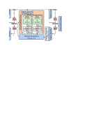
(b)

(c)

(d)

(e)

Figure 2: Illustration of different parallelization techniques for the context modeling in (a) patch-wise grouping [14], (b) checkered grouping [15], (c) channel-wise grouping [16], and (d-e) combination of checkered and channel-wise grouping with sfo and cfo coding, respectively. All latent elements within the same group (depicted with the same color) are coded simultaneously, while the context model aggregates the information from the previously coded groups. For instance, [14, 15] use 2D masked convolutions in the context model, and [16] applies multiple CNNs to channel-wise concatenated groups. The context model of [22] combines the techniques of [16, 15] and can be illustrated as in (d). Our proposed model (eContextformer), as well as the experimental model (pContextformer), use the parallelization techniques depicted in (d–e). However, our models employ spatio-channel attention in context modeling and do not require additional networks for channel-wise concatenation.

II-C Efficient Context Modeling

As an autoregressive context model yields a significant increase of the coding efficiency, multiple architectures have been proposed (see Fig. 1). In our previous study [24], we categorized those into three groups; (1) exploiting spatial dependencies; (2) exploiting cross-channel dependencies; (3) increasing content-adaptive behavior in the entropy estimation.

As an example for the first group, Minnen et al. [5] proposed to use a 2D masked convolution to exploit spatially local relations in the latent space. In order to capture a variety of spatial dependencies, [8, 7] implemented a multi-scale context model using multiple masked convolutions with different kernel sizes. The second group encompasses context models such as 3D context model [6, 10] and channel-wise autoregressive context model [16]. In those proposals, the models are autoregressive in channel dimension, thus they can use information derived from previously coded channels. In [6, 10] the authors use 3D masked convolutions which exploit both spatial and cross-channel dependencies, while the proposal in [16] uses cross-channel dependencies only.

Attention-based models provide better content-adaptivity than the CNN-based ones [23, 12, 17, 24]. Early proposals [23, 12] combine 2D masked convolutions and simplified attention to capture local and global correlations of latent elements. Additionally, Guo et al. [23] propose to split the latent variable into two channel segments to exploit cross-channel relations. Qian et al. [12] capture long-ranged spatial dependencies by transformer-based hyperprior and context model providing adaptive global attention. In a previous work, we proposed a transformer-based context model (a.k.a Contextformer [24]), which splits the latent variable into several channel segments $N_{cs}$ and applies spatio-channel attention. We proposed two different coding modes – spatial-first-order (sfo) and channel-first-order (cfo), which differ in prioritizing spatial and cross-channel correlations.

On the encoder side, all $\bm{\hat{y}_{i}}$ are already available prior to context modeling. Therefore, entropy estimation can be efficiently performed on an NPU/GPU by masking out element permutations which can break coding causality in the sequence. However, in the decoder, entropy modeling requires an autoregresive processing of the latent elements. Such serial processing results in slower decoding time and lower NPU/GPU efficiency. In Fig. 2, we compare techniques which increase parallelization by grouping the elements according to various heuristics [14, 15, 16]. The authors of [14] propose a patch-wise context model processing the latent variable within spatially non-overlapping patches. A multi-scale context model simultaneously exploits the local relations inside each patch. The inter-patch relations are aggregated with an information-sharing block which employs a recurrent neural network. The authors of [15] proposed grouping of the latent variables according to a checkered pattern. They use a 2D masked convolution in context modeling, in which the mask has a checkered pattern. Both [14] and [15] outperform their serial baseline in high bitrates but are inferior to them in low bitrates. In [12], the authors use a transformer-based model with checkered grouping similar to the one used in [15], However, the context model in  [12] has high complexity due to the computation of global attention. The model in [16] is another example of parallel context model, which uses channel-wise grouping. However, it uses separate CNNs to aggregate the decoded channel segments which requires a signifficant number of model parameters. He et al. [22] combined checkered grouping with channel-wise context modeling and reached rate-distortion performance similar to the one of the Contextformer, albeit with a drastically reduced complexity. However, their model uses separate networks to aggregate channels similar to [16] and does not utilize an attention mechanism.

II-D Online Rate-Distortion Optimization

Training a LIC encoder on large datasets gives a set of globally optimal but locally sub-optimal network parameters $(\bm{\phi},\bm{\theta},\bm{\psi})$. For a given input image $x$, a more optimal set of parameters might exist at inference time. Such occurrence is referred to as the amortization gap [43, 44, 33]. The optimization of network parameters per image is not feasible during encoding due to the additional signaling and computational complexity involved in the process. Therefore, [43, 33] propose an online rate distortion optimization (oRDO), which adapts only $\bm{y}$ and $\bm{z}$ during encoding. The oRDO algorithms first initialize the latent variables by passing the input image $\bm{x}$ through the encoder, without tracking the gradients of the transforms. Then, only the latent variables are iteratively optimized using (3a), while network parameters are kept frozen. Finally, the optimized variables $(\bm{\hat{y}_{opt}},\bm{\hat{z}_{opt}})$ are encoded into the bitstream. The oRDO does not influence the decoder complexity or its runtime. However, the iterative process significantly increases the encoder complexity. Therefore, it is primarily implemented on LIC frameworks with low complexity entropy model [4, 5, 11, 9].

III Efficient Contextformer

III-A Exploring Parallelization Techniques

We analyzed the effect of prior parallelization techniques on the Contextformer. We observed a few areas where the architecture design and the training strategy can be improved: (1) overly large kernel size of the attention mechanism; (2) a discrepancy between train and test time behavior; (3) a large number of autoregressive steps. For an input image $\bm{\hat{x}}\in\mathbb{R}^{H\times W\times 3}$ with a latent representation $\bm{\hat{y}}\in\mathbb{R}^{\frac{H}{16}\times\frac{W}{16}\times C}$ (with height $H$, width $W$ and the number of channels $C$), the complexity $\mathbb{C}$ of the Contextformer’s attention mechanism expressed in number of MAC operations is:

$$\mathbb{C}_{\text{attn}} =N_{win}(2N^{2}d_{e}+4N{d_{e}}^{2}),$$ (4a)

$$N_{win} =\frac{HWN_{cs}}{256s^{2}},\quad N=K^{2}N_{cs},$$ (4b)

where the spatial kernel size $K$ and the number of channel segments $N_{cs}$ defines the sequence length $N$ inside a spatio-channel window. The window operation is performed $N_{win}$ times with a stride of $s{=}1$ over $\bm{\hat{y}}$.

Our model is trained with a large spatial kernel ($K{=}16$) on $256{\times}256$ image crops. Therefore, the model learns global attention during training. During inference, it uses sliding window attention, which reduces computational complexity. Compared to global attention used in [12], our sliding window attention provides lower latency. However, our model can not learn the sliding behavior, which creates a discrepancy between training and inference results. This problem could be fixed by training the model with sliding window attention either on larger image crops while using the same kernel size or decreasing the kernel size without changing the image crop size. Training on larger image crops does not affect the complexity and yet increases the compression performance. In this case, direct comparison with prior art trained on small crops would be unfair and would make the effects of parallelization less noticeable. Training with a smaller kernel provides biquadratic complexity reduction for each window. Moreover, the Contextformer requires $N_{win}$ autoregressive steps, which cannot be efficiently implemented on a GPU/NPU. Based on those observations, we built a set of parallel Contextformers (pContextformer), which adopt the patch-wise context [14] and checkerboard context model [15] and need eight autoregressive steps for $N_{cs}{=}4$.

We trained the set of models with $256{\times}256$ image crops for ${\sim}65\%$ of the number of iterations used for training in [24]. We varied the coding method (sfo or cfo), the kernel size $K$, and the stride during training $s_{t}$ and inference $s_{i}$. The stride defines whether the windows are processed in overlapping or separately. To achieve the overlapping window process, we set the stride to $\frac{K}{2}$. For $K{=}16$, the model could learn only global attention, which could be replaced with a local one during the inference. Following the methodology of JPEG-AI [45], we measured the performance of the codec in Bjøntegaard Delta rate (BD-Rate) [46] over VTM 16.2 [29], and the complexity of each context model in kilo MAC operations per pixel (kMAC/px). For simplicity, we measured the single pass complexity in the encoder side, where the whole latent variable $\bm{\hat{y}}$ is processed at once with the given causality mask. We present the results in Fig. 3 and Tables I and II) and make the following observations:

When trained with global attention ($s_{t}{=}K{=}16$)

the spatial-first coding is better than channel-first coding at high bitrates but worse at low bitrates. At low bitrates, the spatial-first coding cannot efficiently exploit spatial dependencies due to the increased sparsity of the latent space, and due to the application of non-overlapping windows during the inference. Also, spatial-first coding benefits more from the overlapping window attention applied at inference time ($s_{i}{<}K$).

Trained with overlapping attention windows ($s_{t}{<}K$)

the spatial-first coding outperforms channel-first coding. Moreover, using overlapping windows at inference time helps the small kernel size models ($K{=}8$) to reach performance close to the one of the larger kernel models ($K{=}16$).

In general

simple pContextformer models can provide more than 100x complexity reduction for a $3\%$ performance drop. Theoretically, more efficient models are possible with the use of overlapping window attention at training and inference time. However, the vanilla version of the overlapping window attention is still sub-optimal since it increases the complexity by four-fold.

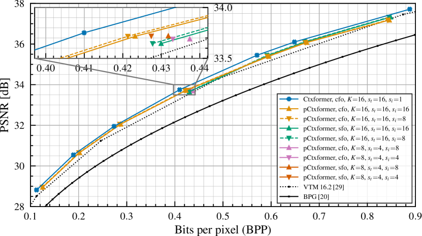
Figure 3: Experimental study on Kodak dataset [30], comparing the rate-distortion performance of different model configurations

III-B Proposed Model

Based on our investigations on vision transformers and initial experiments (see Sections II-A and III-A), we propose Efficient Contextformer (eContextformer) as an improvement to our previous architecture [24]. Built upon the same compression frameworks of [24, 8], the analysis transform $g_{a}$ comprises four $3{\times}3$ convolutional layers with a stride of 2, GDN activation function [47], and a single residual attention module without the non-local mechanism [11, 8, 48], same as in our previous work. The synthesis transform $g_{s}$ closely resembles $g_{a}$ and implements deconvolutional layers with inverse GDN. In order to expand receptive fields and reduce quantization error, $g_{s}$ utilizes residual blocks [6] in its first layer, and a attention module. The entropy model integrates a hyperprior network, universal quantization, and estimates $p_{\bm{\hat{y}_{i}}}(\bm{\hat{y}_{i}}|\bm{\hat{z}})$ with a Gaussian Mixture Model [11] with $k{=}3$ mixtures. In contrast to [24], we use $5{\times}5$ convolutions lieu the $3{\times}3$ ones in the hyperprior in order to align our architecture with the recent state-of-the-art [22, 16].

TABLE I: Rate savings over VTM 16.2 [29] and complexity of various pContextformers with $K{=}16$ compared to [24], showing the effect of coding mode and using overlapped windows during inference

	Coding	Ovp. Win.		BD-Rate
Method	Mode	@Inf.	kMAC/px	[%]
VTM 16.2 [29]	–	–	–	$-$0.0$-$
Contextformer [24]	cfo	✓	$36\cdot 10^{3}$	$-6.9$$-$
pContextformer	cfo		0320	$-3.1$$-$
	cfo	✓	1072	$-3.5$$-$
	sfo		0320	$-1.2$$-$
	sfo	✓	1072	$-1.9$$-$

TABLE II: Performance and complexity of various pContextformers w.r.t. kernel size, coding mode, and using overlapped windows during inference and training

Coding		Ovp. Win.
Order	$K$	@Tr.	@Inf.	kMAC/px	$\Delta$BPP
cfo	8	✓		0195	-0
cfo	8	✓	✓	0710	${\phantom{1}-}4\cdot 10^{-3}$
sfo	8	✓		0195	${\phantom{1}-}6\cdot 10^{-3}$
sfo	8	✓	✓	0710	$-10\cdot 10^{-3}$
cfo	16			0320	$-14\cdot 10^{-3}$
cfo	16		✓	1072	$-16\cdot 10^{-3}$

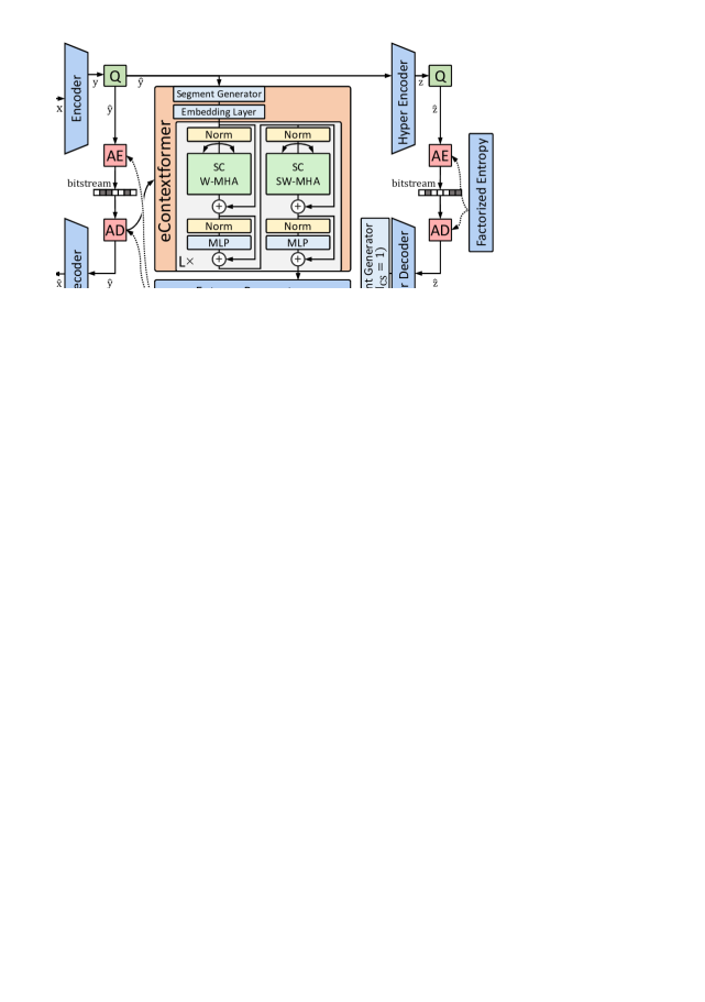
Figure 4: Illustration of our compression framework utilizing with the eContextformer with window and shifted-window spatio-channel attention. The segment generator splits the latent into $N_{cs}$ channel segments for further processing. Following our previous work [24], the output of hyperdecoder is not segmented but repeated along channel dimension to include more channel-wise local neighbors for the entropy modeling.

(a)

(b)

(c)

(d)

(e)

Figure 5: Illustration of the optimized processing steps of eContextformer. From left to right, the latent tensor (a) is first split into channel segments (b) and reordered according to group coding order (c). Finally, the transformer layers with window and shifted-window spatio-channel attention (d-e) are applied on the reordered tensor, sequentially.

Our experiments showed that the Contextformer could support the parallelization techniques of [14, 15], but require an efficient implementation for overlapping window attention. To achieve this, we replaced the ViT-based transformer of Contextformer with a Swin-based one and extended it with the spatio-channel attention. Fig. 4 illustrates our compression framework. For context modeling, the segment generator rearranges the latent $\bm{\hat{y}}\in\mathbb{R}^{H\times W\times C}$ into a spatio-channel segmented representation $\bm{\hat{s}}\in\mathbb{R}^{N_{cs}\times H\times W\times p_{cs}}$ with the number of channel segments $N_{cs}{=}\frac{C}{p_{c}}$. A linear layer converts $\bm{\hat{s}}$ to tensor embedding with the last dimension of $d_{e}$. The embedding representation passes through $L$ Swin transformer layers where window and shifted-window spatio-channel attention (W-SCA and SW-SCA) are applied alternatingly. Window attention is computed on the intermediate outputs with $\mathbb{R}^{N_{w}\times(N_{cs}K^{2})\times p_{cs}}$, where the first and second dimension represents the number of windows $N_{w}{=}\frac{HW}{K^{2}}$ processed in parallel and the sequential data within a window of $K{\times}K$, respectively. We masked each window according to the group coding order (see Fig. 2) to ensure coding causality, where each group uses all the previously coded groups for the context modeling. Following [28], we replaced absolute positional encodings with relative ones to introduce more efficient permutation variance. We employ multi-head attention with $h$ heads to yield better parallelization and build independent relations between different parts of the spatio-channel segments.

III-C Additional Complexity Optimizations

To generate the windows and shifted windows, the transformations $\mathbb{R}^{N_{cs}\times H\times W\times d_{e}}\leftrightarrow\mathbb{R}^{N_{w}\times(N_{cs}K^{2})\times d_{e}}$ are applied to intermediate outputs in pre-post attention layers. Since eContextformer is autoregressive in spatial and channel dimensions, one can iterate over the channel segments with a checkered mask during decoding, i.e., by passing previous segments $\bm{\hat{s}}_{<i}$ through the context model to decode $\bm{\hat{s}}_{i}$ (with the channel segment index $i$). For instance, in spatial-first-order (sfo) setting, two autoregressive steps are required per iteration, while the computation of half of the attention map is unnecessary for each first step. To remedy this, we rearranged the latent tensors into a form $\bm{\hat{r}}\in\mathbb{R}^{2N_{cs}\times H\times\frac{W}{2}\times p_{cs}}$ that is more suitable for efficient processing. We set the window size to $K{\times}\frac{K}{2}$ to preserve the spatial attention span, and applied the window and shifted attention as illustrated in Fig. 5. We refer to the proposed rearrangement operation as Efficient coding Group Rearrangement (EGR). Furthermore, we code the first group $\bm{\hat{r}}_{1}$ only using the hyperprior instead of using a start token for context modeling of $\bm{\hat{r}}_{1}$. This reduced the total autoregressive steps for using the context model to $2N_{cs}-1$, i.e., total complexity reduction of $13\%$ for $N_{cs}{=}4$. We refer to this optimization as Skipping First coding Group (SFG).

Note that transformers are sequence-to-sequence models and compute attention between every query and key-value pair. Let $\bm{Q}(1\leq n)$, $\bm{K}(1\leq n)$ and $\bm{V}(1\leq n)$ be all queries, keys and values, and $Attn(\bm{Q}(1\leq n),\bm{K}(1\leq n),\bm{V}(1\leq n))$ be the attention computed up to coding step $n$. Since context modeling is an autoregressive task, during decoding, one can omit to compute the attention between the previously coded queries and key-value pairs, and just compute the attention $Attn(\bm{Q}(n),\bm{K}(1\leq n),\bm{V}(1\leq n))$ between the current query and the cached key-value pairs. For our efficient implementation, we also adopted the key-value caching according to the white paper [49] and the published work [50].

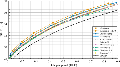
(a)

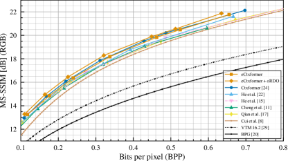
(b)

Figure 6: The rate-distortion performance in terms of (a) PSNR and (b) MS-SSIM on Kodak dataset [30] showing the performance of our model compared to various learning-based and classical codecs. We also include the performance of our model combined with oRDO.

IV Experiments

IV-A Experimental Setup

Training

We configured eContextformer based on the default parameters of the Contextformer [24] $\{N{=}192,\allowbreak\,M{=}192,\,N_{cs}{=}4,\,K{=}8,\,L{=}8,d_{e}{=}\frac{8M}{N_{cs}},\,d_{mlp}{=}4d_{e},\,h{=}12\}$. Here, $N$, $M$, $N_{cs}$, $L$, and $d_{e}$ stand for the intermediate layer size of the encoder and decoder, the bottleneck size, the number of channel segments, the number of layers, embedding size. Since our initial experiments showed deteriorating performance for the $cfo$ coding method for window attention, we continued with the $sfo$ version. $K$ defines the size of the attention span in the spatial dimension, which results in $K{\times}\frac{K}{2}$ window for the proposed optimization algorithms (see Section III-C). Following [24, 51], we trained eContextformer for 120 epochs (${\sim}$1.2M iterations) on $256{\times}256$ random image crops with a batch size of 16 from the Vimeo-90K dataset [52], and used ADAM optimizer [53] with the initial learning rate of $10^{-4}$. In order to cover a range of bitrates, we trained various models with $\lambda\in\{0.002,\,0.004,\,0.007,\,0,014,\,0.026,\,0.034,\,0.058\}$ with mean-squared-error (MSE) as the distortion metric $\mathbf{D}(\cdot)$. To evaluate the perceptual quality of our models, we finetuned them with MS-SSIM [54] as the distortion metric for ${\sim}$500K iterations. For high bitrate models ($\lambda_{5,6,7}$), we increased the bottleneck size to 312 according to the common practice [11, 5, 16]. Empirically, we observed better results with a lower number of heads for the highest rate model, so we reduced it for this model to $h{=}6$. Additionally, we investigated the effect of the training dataset and crop size by finetuning the models with $256{\times}256$ and $384{\times}384$ image crops from COCO 2017 dataset [55] for about ${\sim}$600K iterations.

Evaluation

We analyzed the performance of the eContextformer on the Kodak image dataset [30], CLIC2020 [31] (Professional and Mobile), and Tecnick [32] datasets. We compared its performance to various serial and parallel context models: the 2D context models (Minnen et al. [5] and Cheng et al. [11]), the multi-scale 2D context model (Cui et al. [8]), the 3D context model (Chen et al. [6]), the transformer-based context model with spatio-channel attention (Contextformer [24]), the channel-wise autoregressive context model (Minnen&Singh [16]), the checkerboard context model (He et al. [15]), transformer-based checkerboard context model (Qian et al. [17]), the channel-wise and checkerboard context model (He et al. [22]). If the source was present, we executed the inference algorithms of those methods; otherwise, we obtained the results from relevant publications. Additionally, we also used classical image coding frameworks such as BPG [20] and VTM 16.2 [29] for comparison. We measured the number of parameters of entropy models with the summary functions of PyTorch [56] or Tensorflow [57] (depending on the published implementation). By following the recent standardization activity JPEG-AI [45], we computed the model complexity in kMAC/px with the ptflops package [58]. In case of missing hooks for attention calculation, we integrated them with the help of the official code repository of the Swin transformer [28]. For the runtime measurements, we used DeepSpeed [59] and excluded arithmetic coding time for a fair comparison, since each framework uses different implementation of the arithmetic codec. All the tests, including the runtime measurements, are done on a machine with a single NVIDIA Titan RTX and Intel Core i9-10980XE.

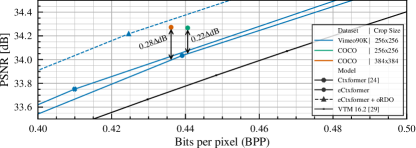
(a)

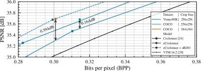
(b)

Figure 7: Experimental study of the effects of different training datasets and crop sizes on the performance, showing the rate-distortion performance on (a) Kodak [30] and (b) Tecnick [32] datasets

IV-B Model Performance

Fig. 6 shows the rate-distortion performance of the eContextformer trained on the Vimeo-90K with $256{\times}256$ image crops. In terms of PSNR, our model qualitatively outperforms the VTM 16.2 [29] for all rate points under test and achieves 5.24% bitrate savings compared to it (see Fig. 6a). Our compression framework shares the same analysis, synthesis transforms, and hyperprior with the model with multi-scale 2D context model [8] and Contextformer [24]. Compared to [8], our model saves 8.5% more bits, while it provides 1.7% lower performance than Contextformer due to the parallelization of context modeling. The eContextformer achieves competitive performance to parallelized models employing channel-wise autoregression with an increased number of model parameters, such as Minnen&Singh [16] and He et al. [22]. When comparing with VTM 16.2 [29], the former model gives 1.6% loss in BD-Rate performance, and the latter gives 6.3% gain.

In Fig. 6b, we also evaluated the perceptually optimized models compared to the prior art. In terms of MS-SSIM [54], the eContextformer saves on average 48.3% bitrate compared to VTM 16.2 [29], which is performance-wise 0.7% better than He et al. [22] and 1.1% worse than the Contextformer [24].

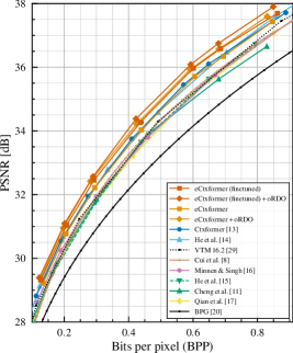
(a)

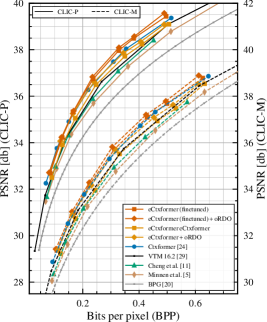
(b)

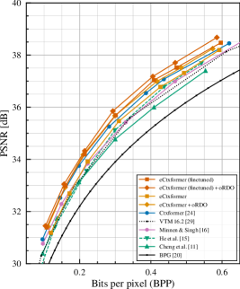
(c)

Figure 8: The rate-distortion performance in terms of PSNR on (a) Kodak [30], (b) CLIC2020 [31] (Professional and Mobile), and (c) Tecnick [32] datasets, showing the performance of our model w/ and w/o finetuning compared to various learning-based and classical codecs. We also include the performance of our models combined with oRDO.

IV-C Effect of training with larger image crops

Although eContextformer yields a performance close to Contextformer on Kodak dataset [30], it underperforms on larger resolution test datasets such as Tecnick [32] (see Fig. 7. The Vimeo-90K dataset [52] we initially used for our training has a resolution of $448{\times}256$. In order to avoid a bias towards horizontal images, we used $256{\times}256$ image crops, ergo $16{\times}16$ latent variable, for training similar to the state-of-the-art [51]. However, the attention window size of $K{=}8$ combined with low latent resolution limits learning an efficient context model. In order to achieve high rate-distortion gain, the recent studies [14, 16, 22, 17] experimented with higher resolution datasets, such as ImageNet [60], COCO 2017 [55], and DIV2K [61], and larger crop sizes up to $512{\times}512$. Following those studies, we finetuned eContextformer with $256{\times}256$ and $384{\times}384$ image crops from COCO 2017 [55]. As one can see in Fig. 7, the models finetuned with different crop sizes achieve similar performance on the Kodak dataset [30], which has about 0.4M pixels. On the contrary, larger crop sizes help the models to reach more than two times increase of performance on the Tecnick dataset [32], which has ${\sim}1.5$M pixels per image.

Fig. 8 shows the rate-distortion performance of t finetuned eContextformer on Kodak [30], CLIC2020 [31] (Professional and Mobile), and Tecnick [32] datasets. The finetuned models provide 5-11% bitrate saving over the initial training, achieving average savings of 10.9%, 12.4%, 6.9% and 12.6% over VTM 16.2 [29] on those datasets, respectively.

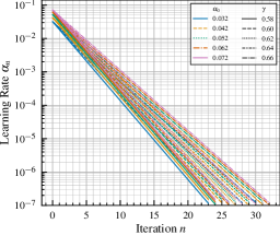
(a)

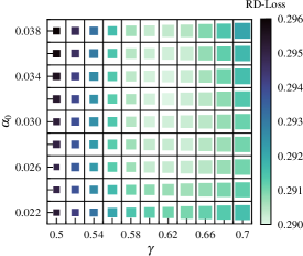
(b)

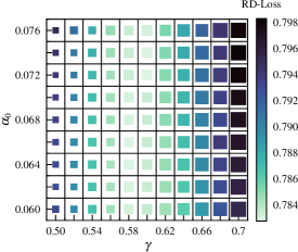
(c)

Figure 9: Illustration of (a) the learning rate decay used for the oRDO w.r.t. optimization iteration for different initial learning rate $\alpha_{0}$ and decay rate $\gamma$. The results of the TPE for our model (b) with $\lambda_{1}$ and (c) with $\lambda_{4}$ for different combinations of $(\alpha_{0},\gamma)$. The size of each square symbolizes the required number of oRDO iteration steps.

IV-D Model and Runtime Complexity

Table III shows the complexity of the eContextformer w.r.t. different optimization proposed in Section III-C. During encoding and decoding, each of the EGR and SFG methods decreases the complexity of context modeling by 10-13%, whereas the combination of them with the caching of key-value pairs provides an 84% complexity reduction in total. We also compared the efficiency of caching to the single pass, where the whole latent variable $\bm{\hat{y}}$ is processed on the encoder side at once with the given causality mask. The caching is also more efficient than the single pass since only the required parts of the attention map are calculated.

In Table IV, we compared the number of model parameters and the complexity of the entropy model (including $g_{c}$, $h_{a}$, $h_{s}$ and $g_{e}$) of our model and some of the prior arts. Compared to the other transformer-based methods, the proposed window attention requires less computation than the sliding window attention of Contextformer and global attention of [17]. For instance, with the proposed optimizations enabled, eContextformer has 145x lower complexity than the Contextformer for a similar number of model parameters. The spatio-channel window attention can efficiently aggregate information of channel segments without concatenation. Therefore, our model requires a smaller and shallower entropy parameter network compared to [8], and a significantly lower total number of parameters in the entropy model compared to channel-wise autoregressive models [16].

TABLE III: Ablation study of the proposed optimization methods applied to eContextformer

EGR	SFG	Single Pass	Caching	kMAC/px
				1200
✓				1075
✓	✓			0829
✓	✓	✓		0212
✓	✓		✓	0204

Table V presents the encoding and decoding runtime complexity of our model, some of the prior learning-based models and VTM 16.2 [29]. The proposed optimizations speed up the encoding and decoding up to 3x, proving a 210x improvement over the optimized version of the Contextformer [24]. Furthermore, we observed that coding time scales better for the optimized eContextformer compared to the one without the proposed optimizations. The 4K images has 21x more pixels than the Kodak images, while the relative encoding and decoding time of the optimized models for those images increase only 14x w.r.t. the ones on the Kodak dataset. Moreover, our optimized model provide competitive runtime performance to the Minnen&Singh [16] and VTM 16.2 [29].

IV-E Online Rate-Distortion Optimization

Since our model with the optimized eContextformer has a significantly low model and runtime complexity on the encoder side, we incorporated an oRDO technique to further improve the compression efficiency. As described in [62], we took the algorithm of [33], replaced the noisy quantization with the straight-through estimator [63], and used an exponential decay for scheduling the learning rate, which results in a simplified oRDO with faster convergence. The learning rate at $n$-th iteration can be defined in closed-form as:

$$\alpha_{n}=\alpha_{0}\gamma^{n},$$ (5)

where $\alpha_{0}$ and $\gamma$ are the initial learning rate and the decay rate, respectively. Fig. 9a illustrates the immediate learning rate $\alpha_{n}$ w.r.t. oRDO steps for different combinations of $(\alpha_{0},\gamma)$.

TABLE IV: Number of parameters and entropy model complexity of our model compared to various various learning-based codecs

	# Parameters $[\text{M}]$		Complexity [kMAC/px]
	Analysis	Entropy	Entropy
Method	& Synthesis	Model	Model
eContextformer (opt.)	17.5	126.9	253
Contextformer [24]	17.5	120.1	$36\cdot 10^{3}$
Cui et al. [8]	17.5	121.8	056
Qian et al. [17]	17.6	129.0	868
Minnen&Singh [16]	18.4	113.5	426
Minnen et al. [5]	15.6	118.3	024

• The complexity is measured on 4K images with 3840x2160 resolution

We searched the optimal parameters by using Tree-Structured Parzen Estimator (TPE) [64] with the objective function (3a) and the constraints of $\alpha_{n}{>}10^{-7}$, $\alpha_{0}\in[0.02,0.08]$, and $\gamma\in[0.5,0.7]$. To omit over-fitting, we used 20 full-resolution images randomly sampled from COCO 2017 dataset [55] for the search. Figs. 9b and 9c show the results of TPE [64] for models trained with $\lambda_{1}$ and $\lambda_{4}$, respectively. We observed that the higher bitrate models ($\lambda_{>3}$) generally perform better with a higher initial learning rate compared to the ones trained for lower bitrates ($\lambda_{<4}$). This suggests that the optimization of less sparse latent space requires a larger step size at each iteration. We set $\alpha_{0}{=}0.062$ and $\gamma{=}0.72$ for $\lambda_{<4}$ and $\alpha_{0}{=}0.062$ and $\gamma{=}0.72$ for $\lambda_{>3}$, which results in 26 iteration steps for all models.

Figs. 6 and 8 show the rate-distortion performance of the eContextformer with oRDO using the optimal parameter setting. Over VTM 16.2 [29], the oRDO increases the rate-distortion performance of the finetuned models up to 4%, providing 14.7%, 14.1%, 10.3%, and 17.1% average bitrate savings on Kodak [30], CLIC2020 [31] (Professional and Mobile), and Tecnick [32] datasets, respectively. The encoding runtime complexity is proportional to the number of optimization steps used. For the selected number of steps, the total encoding runtime complexity of our model is still lower than the VTM 16.2 [29]. Furthermore, we observed that the oRDO increases the performance of our initial models (without the finetuning) by up to 7%, which indicates those models are trained sub-optimally.

TABLE V: Encoding and decoding time of our model compared to various learning-based and classical codecs

	Enc. Time [s]		Dec. Time [s]
Method	Kodak	4K	Kodak	4K
eContextformer	000.33	0006.55	000.35	0006.75
eContextformer (opt.)	000.16	0002.24	000.17	0002.44
Contextformer [24]	056.00	1240.00	062.0	1440.00
Contextformer (opt.) [24]	008.72	0120.00	044.0	0820.00
Chen et al. [6]	004.11	0028.00	316.0	7486.00
Cheng et al. [11]	002.22	0054.00	005.81	0140.00
Qian et al. [17]	001.57	–	002.59	–
Minnen&Singh [16]	000.16	0001.99	000.12	0001.37
VTM 16.2 [29]	420.00	0950.00	000.84	0002.53

V Conclusion

This work introduces eContextformer – an efficient and fast upgrade to the Contextformer. We conduct extensive experimentation to reach a fast and low-complexity context model while presenting state-of-the-art results. Notably, the algorithmic optimizations we provide further reduce the complexity by 84%. Aiming to close the amortization gap, we also experimented with an encoder-side iterative algorithm. It further improves the rate-distortion performance and still has lower complexity than the state-of-art video compression standard. Undoubtedly, there are more advanced compression algorithms yet to be discovered which employ better non-linear transforms and provide more energy-compacted latent space. This work focuses on providing an efficient context model architecture, and defer such an improved transforms to future work.

References

- [1] S. Ma, X. Zhang, C. Jia, Z. Zhao, S. Wang, and S. Wang, “Image and video compression with neural networks: A review,” IEEE Transactions on Circuits and Systems for Video Technology, vol. 30, no. 6, pp. 1683–1698, 2019.
- [2] R. Birman, Y. Segal, and O. Hadar, “Overview of research in the field of video compression using deep neural networks,” Multimedia Tools and Applications, pp. 1–24, 2020.
- [3] J. Ballé, V. Laparra, and E. P. Simoncelli, “End-to-end optimized image compression,” in 5th International Conference on Learning Representations, ICLR 2017, 2017.
- [4] J. Ballé, D. Minnen, S. Singh, S. J. Hwang, and N. Johnston, “Variational image compression with a scale hyperprior,” in International Conference on Learning Representations, 2018.
- [5] D. Minnen, J. Ballé, and G. Toderici, “Joint autoregressive and hierarchical priors for learned image compression,” in NeurIPS, 2018.
- [6] T. Chen, H. Liu, Z. Ma, Q. Shen, X. Cao, and Y. Wang, “End-to-end learnt image compression via non-local attention optimization and improved context modeling,” IEEE Transactions on Image Processing, vol. 30, pp. 3179–3191, 2021.
- [7] J. Zhou, S. Wen, A. Nakagawa, K. Kazui, and Z. Tan, “Multi-scale and context-adaptive entropy model for image compression,” arXiv preprint arXiv:1910.07844, 2019.
- [8] Z. Cui, J. Wang, S. Gao, T. Guo, Y. Feng, and B. Bai, “Asymmetric gained deep image compression with continuous rate adaptation,” in Proceedings of the IEEE/CVF Conference on Computer Vision and Pattern Recognition, 2021, pp. 10 532–10 541.
- [9] J. Lee, S. Cho, and S.-K. Beack, “Context-adaptive entropy model for end-to-end optimized image compression,” in 6th International Conference on Learning Representations, ICLR 2018, 2018.
- [10] F. Mentzer, E. Agustsson, M. Tschannen, R. Timofte, and L. Van Gool, “Conditional probability models for deep image compression,” in Proceedings of the IEEE Conference on Computer Vision and Pattern Recognition, 2018, pp. 4394–4402.
- [11] Z. Cheng, H. Sun, M. Takeuchi, and J. Katto, “Learned image compression with discretized gaussian mixture likelihoods and attention modules,” in Proceedings of the IEEE/CVF Conference on Computer Vision and Pattern Recognition, 2020, pp. 7939–7948.
- [12] Y. Qian, Z. Tan, X. Sun, M. Lin, D. Li, Z. Sun, L. Hao, and R. Jin, “Learning accurate entropy model with global reference for image compression,” in International Conference on Learning Representations, 2020.
- [13] M. Li, K. Ma, J. You, D. Zhang, and W. Zuo, “Efficient and effective context-based convolutional entropy modeling for image compression,” IEEE Transactions on Image Processing, vol. 29, pp. 5900–5911, 2020.
- [14] A. B. Koyuncu, K. Cui, A. Boev, and E. Steinbach, “Parallelized context modeling for faster image coding,” in 2021 International Conference on Visual Communications and Image Processing (VCIP). IEEE, 2021, pp. 1–5.
- [15] D. He, Y. Zheng, B. Sun, Y. Wang, and H. Qin, “Checkerboard context model for efficient learned image compression,” in Proceedings of the IEEE/CVF Conference on Computer Vision and Pattern Recognition, 2021, pp. 14 771–14 780.
- [16] D. Minnen and S. Singh, “Channel-wise autoregressive entropy models for learned image compression,” in 2020 IEEE International Conference on Image Processing (ICIP). IEEE, 2020, pp. 3339–3343.
- [17] Y. Qian, X. Sun, M. Lin, Z. Tan, and R. Jin, “Entroformer: A transformer-based entropy model for learned image compression,” in International Conference on Learning Representations, 2021.
- [18] G. K. Wallace, “The jpeg still picture compression standard,” IEEE transactions on consumer electronics, vol. 38, no. 1, pp. xviii–xxxiv, 1992.
- [19] A. Skodras, C. Christopoulos, and T. Ebrahimi, “The jpeg 2000 still image compression standard,” IEEE Signal processing magazine, vol. 18, no. 5, pp. 36–58, 2001.
- [20] F. Bellard, “Bpg image format,” 2015, https://bellard.org/bpg (accessed Dec. 01, 2022).
- [21] V. Sze, M. Budagavi, and G. J. Sullivan, “High efficiency video coding (hevc),” in Integrated circuit and systems, algorithms and architectures. Springer, 2014, vol. 39, p. 40.
- [22] D. He, Z. Yang, W. Peng, R. Ma, H. Qin, and Y. Wang, “Elic: Efficient learned image compression with unevenly grouped space-channel contextual adaptive coding,” in Proceedings of the IEEE/CVF Conference on Computer Vision and Pattern Recognition, 2022, pp. 5718–5727.
- [23] Z. Guo, Z. Zhang, R. Feng, and Z. Chen, “Causal contextual prediction for learned image compression,” IEEE Transactions on Circuits and Systems for Video Technology, 2021.
- [24] A. B. Koyuncu, H. Gao, A. Boev, G. Gaikov, E. Alshina, and E. Steinbach, “Contextformer: A transformer with spatio-channel attention for context modeling in learned image compression,” in Computer Vision–ECCV 2022: 17th European Conference, Tel Aviv, Israel, October 23–27, 2022, Proceedings, Part XIX. Springer, 2022, pp. 447–463.
- [25] “Versatile Video Coding,” Rec. ITU-T H.266 and ISO/IEC 23090-3, Standard, Aug. 2020.
- [26] J. Ballé, P. A. Chou, D. Minnen, S. Singh, N. Johnston, E. Agustsson, S. J. Hwang, and G. Toderici, “Nonlinear transform coding,” IEEE Journal of Selected Topics in Signal Processing, vol. 15, no. 2, pp. 339–353, 2020.
- [27] C. C. Chi, M. Alvarez-Mesa, B. Juurlink, G. Clare, F. Henry, S. Pateux, and T. Schierl, “Parallel scalability and efficiency of hevc parallelization approaches,” IEEE Transactions on circuits and systems for video technology, vol. 22, no. 12, pp. 1827–1838, 2012.
- [28] Z. Liu, Y. Lin, Y. Cao, H. Hu, Y. Wei, Z. Zhang, S. Lin, and B. Guo, “Swin transformer: Hierarchical vision transformer using shifted windows,” in Proceedings of the IEEE/CVF international conference on computer vision, 2021, pp. 10 012–10 022.
- [29] J. V. E. Team, “Versatile video coding (vvc) reference software: Vvc test model (vtm),” 2022, https://vcgit.hhi.fraunhofer.de/jvet/VVCSoftware_VTM (accessed Dec. 01, 2022).
- [30] R. Franzen, “Kodak lossless true color image suite,” 1999.
- [31] G. Toderici, L. Theis, N. Johnston, E. Agustsson, F. Mentzer, J. Ballé, W. Shi, and R. Timofte, “Workshop and challenge on learned image compression (clic2020).”
- [32] N. Asuni and A. Giachetti, “Testimages: a large-scale archive for testing visual devices and basic image processing algorithms.” in STAG, 2014, pp. 63–70.
- [33] J. Campos, S. Meierhans, A. Djelouah, and C. Schroers, “Content adaptive optimization for neural image compression,” in Proceedings of the IEEE/CVF Conference on Computer Vision and Pattern Recognition Workshops, 2019, pp. 0–0.
- [34] A. Vaswani, N. Shazeer, N. Parmar, J. Uszkoreit, L. Jones, A. N. Gomez, Ł. Kaiser, and I. Polosukhin, “Attention is all you need,” in Advances in neural information processing systems, 2017, pp. 5998–6008.
- [35] A. Krizhevsky, I. Sutskever, and G. E. Hinton, “Imagenet classification with deep convolutional neural networks,” in Advances in Neural Information Processing Systems, F. Pereira, C. Burges, L. Bottou, and K. Weinberger, Eds., vol. 25. Curran Associates, Inc., 2012. [Online]. Available: https://proceedings.neurips.cc/paper_files/paper/2012/file/c399862d3b9d6b76c8436e924a68c45b-Paper.pdf
- [36] M. M. Naseer, K. Ranasinghe, S. H. Khan, M. Hayat, F. Shahbaz Khan, and M.-H. Yang, “Intriguing properties of vision transformers,” Advances in Neural Information Processing Systems, vol. 34, pp. 23 296–23 308, 2021.
- [37] N. Carion, F. Massa, G. Synnaeve, N. Usunier, A. Kirillov, and S. Zagoruyko, “End-to-end object detection with transformers,” in European Conference on Computer Vision. Springer, 2020, pp. 213–229.
- [38] A. Dosovitskiy, L. Beyer, A. Kolesnikov, D. Weissenborn, X. Zhai, T. Unterthiner, M. Dehghani, M. Minderer, G. Heigold, S. Gelly et al., “An image is worth 16x16 words: Transformers for image recognition at scale,” in International Conference on Learning Representations, 2020.
- [39] Y. Jiang, S. Chang, and Z. Wang, “Transgan: Two transformers can make one strong gan,” arXiv preprint arXiv:2102.07074, 2021.
- [40] P. Esser, R. Rombach, and B. Ommer, “Taming transformers for high-resolution image synthesis,” in Proceedings of the IEEE/CVF Conference on Computer Vision and Pattern Recognition, 2021, pp. 12 873–12 883.
- [41] N. Parmar, A. Vaswani, J. Uszkoreit, L. Kaiser, N. Shazeer, A. Ku, and D. Tran, “Image transformer,” in International Conference on Machine Learning. PMLR, 2018, pp. 4055–4064.
- [42] J. Rissanen and G. G. Langdon, “Arithmetic coding,” IBM Journal of research and development, vol. 23, no. 2, pp. 149–162, 1979.
- [43] Y. Yang, R. Bamler, and S. Mandt, “Improving inference for neural image compression,” Advances in Neural Information Processing Systems, vol. 33, pp. 573–584, 2020.
- [44] C. Gao, T. Xu, D. He, Y. Wang, and H. Qin, “Flexible neural image compression via code editing,” Advances in Neural Information Processing Systems, vol. 35, pp. 12 184–12 196, 2022.
- [45] J. Ascenso, E. Alshina, and T. Ebrahimi, “The jpeg ai standard: Providing efficient human and machine visual data consumption,” IEEE MultiMedia, vol. 30, no. 1, pp. 100–111, 2023.
- [46] G. Bjontegaard, “Calculation of average psnr differences between rd-curves,” VCEG-M33, 2001.
- [47] J. Ballé, V. Laparra, and E. P. Simoncelli, “Density modeling of images using a generalized normalization transformation,” in 4th International Conference on Learning Representations, ICLR 2016, 2016.
- [48] Y. Zhang, K. Li, K. Li, B. Zhong, and Y. Fu, “Residual non-local attention networks for image restoration,” in International Conference on Learning Representations, 2019. [Online]. Available: https://openreview.net/forum?id=HkeGhoA5FX
- [49] A. Matton and A. Lam, “Making pytorch transformer twice as fast on sequence generation.” 2020, https://scale.com/blog/pytorch-improvements (accessed Dec. 01, 2022).
- [50] Y. Yan, F. Hu, J. Chen, N. Bhendawade, T. Ye, Y. Gong, N. Duan, D. Cui, B. Chi, and R. Zhang, “Fastseq: Make sequence generation faster,” in Proceedings of the 59th Annual Meeting of the Association for Computational Linguistics and the 11th International Joint Conference on Natural Language Processing: System Demonstrations, 2021, pp. 218–226.
- [51] J. Bégaint, F. Racapé, S. Feltman, and A. Pushparaja, “Compressai: a pytorch library and evaluation platform for end-to-end compression research,” arXiv preprint arXiv:2011.03029, 2020.
- [52] T. Xue, B. Chen, J. Wu, D. Wei, and W. T. Freeman, “Video enhancement with task-oriented flow,” International Journal of Computer Vision (IJCV), vol. 127, no. 8, pp. 1106–1125, 2019.
- [53] D. P. Kingma and J. Ba, “Adam: A method for stochastic optimization,” arXiv preprint arXiv:1412.6980, 2014.
- [54] Z. Wang, E. P. Simoncelli, and A. C. Bovik, “Multiscale structural similarity for image quality assessment,” in The Thrity-Seventh Asilomar Conference on Signals, Systems & Computers, 2003, vol. 2. Ieee, 2003, pp. 1398–1402.
- [55] T.-Y. Lin, M. Maire, S. Belongie, J. Hays, P. Perona, D. Ramanan, P. Dollár, and C. L. Zitnick, “Microsoft coco: Common objects in context,” in Computer Vision–ECCV 2014: 13th European Conference, Zurich, Switzerland, September 6-12, 2014, Proceedings, Part V 13. Springer, 2014, pp. 740–755.
- [56] A. Paszke, S. Gross, F. Massa, A. Lerer, J. Bradbury, G. Chanan, T. Killeen, Z. Lin, N. Gimelshein, L. Antiga, A. Desmaison, A. Kopf, E. Yang, Z. DeVito, M. Raison, A. Tejani, S. Chilamkurthy, B. Steiner, L. Fang, J. Bai, and S. Chintala, “Pytorch: An imperative style, high-performance deep learning library,” in Advances in Neural Information Processing Systems 32. Curran Associates, Inc., 2019, pp. 8024–8035. [Online]. Available: http://papers.neurips.cc/paper/9015-pytorch-an-imperative-style-high-performance-deep-learning-library.pdf
- [57] M. Abadi et al., “TensorFlow: Large-scale machine learning on heterogeneous systems,” 2015, software available from tensorflow.org. [Online]. Available: https://www.tensorflow.org/
- [58] V. Sovrasov. (2018-2023) ptflops: a flops counting tool for neural networks in pytorch framework. [Online]. Available: https://github.com/sovrasov/flops-counter.pytorch
- [59] J. Rasley, S. Rajbhandari, O. Ruwase, and Y. He, “Deepspeed: System optimizations enable training deep learning models with over 100 billion parameters,” in Proceedings of the 26th ACM SIGKDD International Conference on Knowledge Discovery & Data Mining, 2020, pp. 3505–3506.
- [60] J. Deng, W. Dong, R. Socher, L.-J. Li, K. Li, and L. Fei-Fei, “Imagenet: A large-scale hierarchical image database,” in 2009 IEEE conference on computer vision and pattern recognition. Ieee, 2009, pp. 248–255.
- [61] E. Agustsson and R. Timofte, “Ntire 2017 challenge on single image super-resolution: Dataset and study,” in Proceedings of the IEEE conference on computer vision and pattern recognition workshops, 2017, pp. 126–135.
- [62] E. Alshina, A. Boev, P. Jia, A. B. Koyuncu, E. Koyuncu, A. Karabutov, T. Solovyev, J. Sauer, M. Sychev, G. Gaikov, T. Guo, Y. Feng, Z. Cui, J. Mao, S. Qian, J. Wang, D. Yu, Y. Zhao, and M. Li, “Presentation of the Huawei response to the JPEG AI Call for Proposals: Device agnostic learnable image coding using primary component extraction and conditional coding,” Huawei Technologies, Tech. Rep. wg1m96016-REQ, 2022. [Online]. Available: https://sd.iso.org/documents/ui/#!/doc/4fedde90-6234-4aa4-9ecb-331f08e90245
- [63] Y. Bengio, N. Léonard, and A. Courville, “Estimating or propagating gradients through stochastic neurons for conditional computation,” arXiv preprint arXiv:1308.3432, 2013.
- [64] J. Bergstra, R. Bardenet, Y. Bengio, and B. Kégl, “Algorithms for hyper-parameter optimization,” Advances in neural information processing systems, vol. 24, 2011.