CP asymmetries in $B$ meson two-body baryonic decays

Abstract

We study the CP-odd and CP-even observables of the $B$ mesons decaying into a baryon and antibaryon. We estimate these observables through the ${}^{3}P_{0}$ model and chiral selection rule. The decay branching ratios of $B^{+}\to p\overline{\Lambda}$ and $B^{0}\to p\overline{p}$ are calculated to be $2.31\times 10^{-7}$ and $1.27\times 10^{-8}$, which are consistent with the current experiments, respectively. The effects of the $B-\overline{B}$ oscillations are considered, which largely suppress the direct CP asymmetries in the $B_{s}^{0}$ decays. We suggest the experiments to visit $B_{s}^{0}\to\Lambda(\to p\pi^{-})\overline{\Lambda}(\to\overline{p}\pi^{+})$, where the time-averaged CP-odd observables are estimated to be large. The direct CP asymmetries of $B^{+}\to p\overline{\Lambda}$ and $B^{0}\to p\overline{p}$ are found to be $26.2\%$ and $-3.1\%$ for a positive strong phase and $-36.9\%$ and $4.2\%$ for a negative strong phase, respectively.

I Introduction

CP asymmetries play an important role in the study of particle physics CPNP . In particular, CP violation is not only the key to understand the matter-antimatter asymmetry in the universe but an important way to probe the effects of new physics (NP). As the CP symmetry is respected by the strong interaction, the study of CP violation allows us to extract the complex phases in the weak interaction of the standard model (SM) Gronau:1990ra ; CKM ; LHCb:2017hkl ; Geng:2022osc even though theoretical calculations are clouded by the hadronic uncertainties.

Since CP violation was first observed in 2001 BCP , various CP-odd quantities have been measured mainly in the $B$ meson decays pdg . Remarkably, the LHCb collaboration has recently found evidences of CP violation in $D$ meson decays LHCb:2014kcb , which are expected to be small. The finding has stimulated great interests among the theorist and a debate on whether the observed values require NP is still ongoing DmesonCP .

Despite the great processes in the mesonic sector, a nonzero signal at $5\sigma$ confidential level of CP violation is still absent in the baryonic sector yet. In particular, the direct CP violation of $\Lambda_{b}\to\Lambda K^{-}\pi^{+}$ is found to be $-0.53\pm 0.25$ LHCb:2016rja , which has a huge central value but a large uncertainty. In addition, several theoretical works PQCD have been triggered by the measurements of $A_{CP}(\Lambda_{b}\to p\pi^{-}/K^{-})$, which are consistent with the results in the perturbative QCD (pQCD) private . Undoubtedly, more experiments are expected in the future.

To the end of probing CP violation involving baryons, we study the CP asymmetries exhibit in $B\to{\bf B}_{1}\overline{{\bf B}}_{2}$ with ${\bf B}_{1}$ and $\overline{{\bf B}}_{2}$ baryon and antibaryon, respectively. On the one hand, it benefits by the simplicity of the two-body decays. On the other, the spins of ${\bf B}_{1}$ and $\overline{{\bf B}}_{2}$ provide fruitful physical observables in experiments. Additionally, the production rate of $B$ is roughly three times larger than the one of the bottom baryons ProductionRate , making $B\to{\bf B}_{1}\overline{{\bf B}}_{2}$ an ideal place to probe CP violation with baryons. We note that the direct CP asymmetries in $B\to{\bf B}_{1}\overline{{\bf B}}_{2}$ have systematically estimated by Ref. Chua:2022wmr but the $B$ meson oscillation and CP asymmetries in angular distributions have not been considered yet.

The LHCb collaboration have measured the branching ratios of LHCb:2016nbc ; LHCb:2022lff ,

$${\cal B}(B^{+}\to p\overline{\Lambda})=\left(2.4_{-0.8}^{+1.0}\pm 0.3\right)\times 10^{-7}\,,~{}~{}~{}{\cal B}(B^{0}\to p\overline{p})=(1.27\pm 0.14)\times 10^{-8}\,,$$ (1)

and obtained a upper limit of LHCb:2022lff ,

$${\cal B}(B_{s}^{0}\to p\overline{p})<5.1\times 10^{-9}\,,$$ (2)

at 95$\%$ confidence level, which is consistent with ${\cal B}(B_{s}^{0}\to p\overline{p})<1\times 10^{-10}$ predicted by the chiral selection rule Jin:2021onb ; Chua:2022wmr . In the theoretical studies, the calculated amplitudes depend heavily on QCD models, such as the pole model Cheng:2001ub and sum rule Chernyak:1990ag . Nevertheless, in the literature ${\cal B}(B^{0}\to p\overline{p})$ is overestimated by an order. The reason behind it is closely related to the Fierz identity Cheng:2014qxa .

This paper is organized as follows. In Sec. II, we define the decay parameters associated with spins and classify them in terms of CP-odd or CP-even parts. In Sec. III, we analyze the decay distributions of $B\to{\bf B}_{1}\overline{{\bf B}}_{2}$. In Sec. IV, we estimate the decay parameters through the ${}^{3}P_{0}$ model and chiral selection rule. Our numerical results are shown in Sec. V. Sec. VI is devoted to conclusions.

II Decay parameters

In general, with $\hat{A}$ an arbitrary Hermitian operator, we can define a corresponding asymmetry as

$$~{}A\equiv\frac{\Gamma(\lambda_{A}>0)-\Gamma(\lambda_{A}<0)}{\Gamma(\lambda_{A}>0)+\Gamma(\lambda_{A}<0)}\,,$$ (3)

where $\Gamma$ represents the decay width, and $\lambda_{A}$ stands for the eigenvalue of $\hat{A}$. In decay final states, it is convenient to choose $\hat{A}$ as an $SO(3)$ rotational scalar, since the angular momenta are always constrained by the spins of the parent particles. In $B\to{\bf B}_{1}\overline{{\bf B}}_{2}$, we simply have $J=0$ and the most simple operators are

$$\hat{\alpha}=\vec{s}_{1}\cdot\hat{p}\,,\,\,\,\,\,\,\,\hat{\beta}=(\vec{s}_{1}\times\vec{s}_{2})\cdot\hat{p}\,,\,\,\,\,\,\,\,\hat{\gamma}=2\,\vec{s}_{1}\cdot\vec{s}_{2}\,,$$ (4)

where $\vec{s}_{1}~{}(\vec{s}_{2})$ is the spin operator of ${\bf B}_{1}~{}(\overline{{\bf B}}_{2})$, and $\hat{p}$ is the 3-momentum norm of ${\bf B}_{1}$. From Eqs. (3) and (4), we define

$$\alpha\equiv\frac{\Gamma(\lambda_{\alpha}>0)-\Gamma(\lambda_{\alpha}<0)}{\Gamma(\lambda_{\alpha}>0)+\Gamma(\lambda_{\alpha}<0)}\,,\,\,\,\,\,\beta\equiv\frac{\Gamma(\lambda_{\beta}>0)-\Gamma(\lambda_{\beta}<0)}{\Gamma(\lambda_{\beta}>0)+\Gamma(\lambda_{\beta}<0)}\,,\,\,\,\,\,\gamma\equiv\frac{\Gamma(\lambda_{\gamma}>0)-\Gamma(\lambda_{\gamma}<0)}{\Gamma(\lambda_{\gamma}>0)+\Gamma(\lambda_{\gamma}<0)}\,,$$ (5)

which affect the cascade decay distributions as we will demonstrate in the next section. Clearly, $\hat{\alpha}$ is a helicity operator and $\hat{\beta}$ describes the T-odd spin correlation.

Since $\hat{\alpha}$ and $\hat{\beta}$ are both P-odd, $\lambda_{\alpha}$ and $\lambda_{\beta}$ would flip signs under the parity transformation. On the other hand, $\hat{\beta}$ is T-odd and $\beta$ is a naively T-odd observable. In general, a nonzero value of $\beta$ can be generated by the oscillations between $|\pm\lambda_{\beta}\rangle$ with the final state interactions. We utilize the CPT symmetry and define the true T-odd observables as

$$\beta_{w}=(\beta\Gamma+\overline{\beta}\,\overline{\Gamma})/(\Gamma+\overline{\Gamma})\,,$$ (6)

where overlines denote the charge conjugates. We emphasize that $\beta_{w}$ is clearly also a CP violating observable. The other CP violating observables can be defined to be

$${\cal A}_{\text{dir}}=(\Gamma-\overline{\Gamma})/(\Gamma+\overline{\Gamma})\,,~{}~{}~{}~{}\alpha_{w}=(\alpha\Gamma+\overline{\alpha}\,\overline{\Gamma})/(\Gamma+\overline{\Gamma})\,,~{}~{}~{}~{}\gamma_{w}=(\gamma\Gamma-\overline{\gamma}\,\overline{\Gamma})/(\Gamma+\overline{\Gamma})\,,$$ (7)

where the signs of Eqs. (6) and (7) are according to the parity of the responsible operators. To be explicit, $\hat{\alpha}$ and $\hat{\beta}$ are both P-odd, leading to the plus signs, whereas $\hat{\gamma}$ is P-even, resulting in the minus sign. On the other hand, the CP-even observables are

$$\beta_{s}=(\beta\Gamma-\overline{\beta}\,\overline{\Gamma})/(\Gamma+\overline{\Gamma})\,,\quad\alpha_{s}=(\alpha\Gamma-\overline{\alpha}\,\overline{\Gamma})/(\Gamma+\overline{\Gamma})\,,\quad\gamma_{s}=(\gamma\Gamma+\overline{\gamma}\,\overline{\Gamma})/(\Gamma+\overline{\Gamma})\,,$$ (8)

where the subscripts of $w$ and $s$ denote CP-odd and CP-even, respectively.

Clearly, to calculate the asymmetries in Eq. (3), it is necessary to obtain the eigenstates of $\hat{\alpha},~{}\hat{\beta}$ and $\hat{\gamma}$. To this end, we start with $\hat{\alpha}$ and express the others in the linear combinations of $|\lambda_{\alpha}\rangle$. With $J=0$ , the helicity states are given as

$$|\lambda_{\alpha}=\pm 1/2\rangle=\int^{2\pi}_{0}\int^{1}_{-1}R_{z}(\phi)R_{y}(\theta)\left|\hat{p}=\hat{z},\lambda_{1}=\lambda_{2}=\pm 1/2\right\rangle d\cos\theta d\phi\,,$$ (9)

where $\lambda_{1(2)}$ is the helicity of ${\bf B}_{1}~{}(\overline{{\bf B}}_{2})$, and $R_{i}$ is the rotational operator pointing toward the $i$th direction. Note that the operators in Eq. (4) commute with $R_{i}$ and BVV

$$(s_{j})_{\pm}|\hat{p}=\hat{z},\lambda_{j}=\mp 1/2\rangle=|\hat{p}=\hat{z},\lambda_{j}=\pm 1/2\rangle\,\,\,\,\,\,\,\,\text{for}~{}~{}j\in\{1,2\}\,,$$ (10)

with $(s_{j})_{\pm}=(s_{j})_{x}\pm i(s_{j})_{y}$. Together with Eqs. (4), (9) and (10), the eigenstates of $\hat{\beta}$ and $\hat{\gamma}$ are then given as

$$|\lambda_{\beta}=\pm 1/2\rangle = \frac{1}{\sqrt{2}}\left(|\lambda_{\alpha}=1/2\rangle\mp i|\lambda_{\alpha}=-1/2\rangle\right)\,,$$

$$|\lambda_{\gamma}=\pm 1/2\rangle = \frac{1}{\sqrt{2}}\left(|\lambda_{\alpha}=1/2\rangle\pm|\lambda_{\alpha}=-1/2\rangle\right)\,.$$ (11)

The asymmetry parameters defined in Eq. (3) are then given as

$$\alpha=\frac{|H_{+}|^{2}-|H_{-}|^{2}}{|H_{+}|^{2}+|H_{-}|^{2}}\,,\,\,\,\,\,\,\,\beta=\frac{2\Im(H_{-}^{*}H_{+})}{|H_{+}|^{2}+|H_{-}|^{2}}\,,\,\,\,\,\,\,\,\gamma=\frac{2\Re(H_{-}^{*}H_{+})}{|H_{+}|^{2}+|H_{-}|^{2}}\,,$$ (12)

with the identity

$$1-\left(\alpha^{2}+\beta^{2}+\gamma^{2}\right)=0\,.$$ (13)

Here, $H_{\pm}$ stand for the helicity amplitudes, defined by

$$H_{\pm}=\langle\lambda_{\alpha}=\pm 1/2|i{\cal H}_{eff}|B\rangle=\sum_{j}H^{\pm}_{j}\exp\left(i\phi_{j_{s}}^{\pm}+i\phi_{j_{w}}^{\pm}\right)\,,$$ (14)

where ${\cal H}_{eff}$ is the effective Hamiltonian, $H_{j}^{\pm}$ are real, and $\phi^{j_{s}}_{\pm}$ and $\phi^{j_{w}}_{\pm}$ are the strong and the weak CP phases, respectively. The charge conjugate ones can be obtained by taking the CP transformation

$$\overline{H}_{\mp}=\langle\lambda_{\alpha}=\mp 1/2|i{\cal H}_{eff}|\overline{B}\rangle=\sum_{j}H^{\pm}_{j}\exp\left(i\phi_{j_{s}}^{\pm}-i\phi_{j_{w}}^{\pm}\right)\,.$$ (15)

Notice that $\lambda_{\alpha}$ flips sign after the CP transformation.

For $B_{(s)}^{0}$, the decay parameters in Eq. (12) depend on time due to the $B-\overline{B}$ mixing, given by

$$|B^{0}_{(s)}(t)\rangle=g_{+}(t)|B_{(s)}^{0}(t=0)\rangle+\frac{q}{p}g_{-}(t)|\overline{B}_{(s)}^{0}(t=0)\rangle\,,$$

$$|\overline{B}^{0}_{(s)}(t)\rangle=\frac{p}{q}g_{-}(t)|B_{(s)}^{0}(t=0)\rangle+g_{+}(t)|\overline{B}_{(s)}^{0}(t=0)\rangle\,,$$ (16)

where $p$ and $q$ are the mixing parameters, and

$$g_{+}(t)\pm g_{-}(t)=e^{\left(-\Gamma\mp\Delta\Gamma/2\right)t/2}e^{-i\left(M\pm\Delta M/2\right)t}\,.$$ (17)

The parameters associated with the masses and the decay widths are defined as

$$M=(M_{H}+M_{L})/2\,,\quad\Gamma=(\Gamma_{H}+\Gamma_{L})/2\,,$$

$$M_{\Delta}=M_{H}-M_{L}\,,\quad\Gamma_{\Delta}=\Gamma_{L}-\Gamma_{H}\,,$$ (18)

where $m_{L,H}$ and $\Gamma_{L,H}$ are the masses and total decay widths of the light and heavy neutral $B$ mesons, respectively. Clearly, $g_{\pm}(t)$, $M_{H,L}$ and $\Gamma_{H,L}$ depend on whether $B^{0}$ or $B^{0}_{s}$ is in question. We do not explicitly show the dependence as long as it does not cause confusion. In this work, we take $q=p$, corresponding to that CP is conserved in the oscillations, which causes some errors at the $O(10^{-3})$ level. In the future studies, the approximation is not necessary if a higher precision is desired.

Using Eqs. (II) and (21), we arrive at

$$\langle\lambda_{\alpha}=\pm 1/2|i{\cal H}_{eff}|B^{0}_{(s)}(t)\rangle=g_{+}(t)H_{\pm}+g_{-}(t)\overline{H}_{\pm}\,,$$

$$\langle\lambda_{\alpha}=\pm 1/2|i{\cal H}_{eff}|\overline{B}^{0}_{(s)}(t)\rangle=g_{+}(t)\overline{H}_{\pm}+g_{-}(t)H_{\pm}\,,$$ (19)

leading to

$$D(t) = (|g_{+}|^{2}+|g_{-}^{2}|)D+4\Re(g_{+}g_{-}^{*})\left(\Re(H_{+}\overline{H}_{+}^{*}+H_{-}\overline{H}_{-}^{*})\right)$$

$${\cal A}_{\text{dir}}(t) = \left[(|g_{+}|^{2}-|g_{-}|^{2}){\cal A}_{\text{dir}}(0)D+4\Im(g_{+}g_{-}^{*})\left(\Im(H_{+}\overline{H}_{+}^{*}+H_{-}\overline{H}_{-}^{*})\right)\right]/D(t)\,,$$

$$\alpha_{s}(t) = \left[(|g_{+}|^{2}-|g_{-}|^{2})\alpha_{s}(0)D+4\Im(g_{-}g_{+}^{*})\left(\Im(H_{+}\overline{H}_{+}^{*}-H_{-}\overline{H}_{-}^{*})\right)\right]/D(t)\,,$$

$$\alpha_{w}(t) = \left[(|g_{+}|^{2}+|g_{-}|^{2})\alpha_{w}(0)D+4\Re(g_{+}g_{-}^{*})\left(\Re(H_{+}\overline{H}_{+}^{*}-H_{-}\overline{H}_{-}^{*})\right)\right]/D(t)\,,$$

$$\beta_{s}(t) = \left[(|g_{+}|^{2}-|g_{-}|^{2})\beta_{s}(0)D+4\Im(g_{+}^{*}g_{-})\left(\Re(H_{-}^{*}\overline{H}_{+}-H_{+}\overline{H}_{-}^{*})\right)\right]/D(t)\,,$$

$$\beta_{w}(t) = \left[(|g_{+}|^{2}+|g_{-}|^{2})\beta_{w}(0)D+4\Re(g_{+}^{*}g_{-})\left(\Im(H_{-}^{*}\overline{H}_{+}+H_{+}\overline{H}_{-}^{*})\right)\right]/D(t)\,,$$

$$\gamma_{s}(t) = \left[(|g_{+}|^{2}+|g_{-}|^{2})\gamma_{s}(0)D+4\Re(g_{-}g_{+}^{*})\left(\Re(H_{-}^{*}\overline{H}_{+}+H_{+}\overline{H}_{-}^{*})\right)\right]/D(t)\,,$$

$$\gamma_{w}(t) = \left[(|g_{+}|^{2}-|g_{-}|^{2})\gamma_{w}(0)D-4\Im(g_{-}g_{+}^{*})\left(\Im(H_{-}^{*}\overline{H}_{+}-H_{+}\overline{H}_{-}^{*})\right)\right]/D(t)\,,$$ (20)

where the denominator is $D=|H_{+}|^{2}+|H_{-}|^{2}+|\overline{H}_{+}|^{2}+|\overline{H}_{-}|^{2}$. In the experiments, the measured quantities correspond to the ones averaged from $t_{1}$ to $t_{2}$. By taking $t_{1}=0$ and $t_{2}\to\infty$, we find that

$$\langle|g_{+}|^{2}+|g_{-}|^{2}\rangle=\frac{1}{\Gamma}\frac{4}{4-x^{2}}\,,\qquad\langle|g_{+}|^{2}-|g_{-}|^{2}\rangle=\frac{1}{\Gamma}\frac{1}{1+y^{2}}\,,$$ (21)

$$\langle g_{+}(t)g_{-}^{*}(t)\rangle=\frac{1}{\Gamma}\left(\frac{-x}{4-x^{2}}-\frac{iy}{1+y}\right)\,,$$

with $(x,y)=(\Gamma_{\Delta}/\Gamma,M_{\Delta}/\Gamma)$. In this work, the values of the oscillating parameters are from the Particle Data Group (PDG) pdg , given by

$$(x,y)_{B_{0}}=(0.001,0.77), (x,y)_{B_{s}^{0}}=(0.128,27)\,.$$ (22)

III angular distributions

From Eq. (9), the decay distributions of $B\to{\bf B}_{1}\overline{{\bf B}}_{2}$ are trivial since $B$ is spinless. Hence, the asymmetry parameters defined in Eq. (12) are essentially described by the spin correlations between ${\bf B}_{1}$ and $\overline{{\bf B}}_{2}$. In the LHCb experiments, spins can not be measured directly and we therefore shall seek the spin effects in their cascade decays.

If ${\bf B}_{1}\in\{\Xi^{0,-},\Sigma^{\pm},\Lambda\}$, it would consequently decay to an octet baryon $({\bf B}_{1}^{\prime})$ and a pion, while $H_{\pm}$ interfere via the cascade decays. The partial decay widths are proportional to

$$\frac{\partial\Gamma}{\partial\cos\theta_{1}}\propto\sum_{\lambda_{1}}\left|\sum_{\lambda}H_{\lambda}A_{1,\lambda_{1}}d^{\frac{1}{2}}(\theta_{1})^{\lambda}\,_{\lambda_{1}}\right|^{2}\,,$$ (23)

with $\theta_{1}$ defined as the polar angles in the ${\bf B}_{1}$ helicity frame (see FIG. 1), resulting in

$${\cal D}_{1}(\theta_{1})\equiv\frac{1}{\Gamma}\frac{\partial\Gamma}{\partial\cos\theta_{1}}=\frac{1}{2}\left(1+\alpha\alpha_{1}\cos\theta_{1}\right)\,,$$ (24)

where we have used $\left|A_{1,\pm}\right|^{2}=(1\pm\alpha_{1})/2$ in the last equation with $\alpha_{1}$ the up-down asymmetry parameter for ${\bf B}_{1}\to{\bf B}_{1}^{\prime}\pi$, and $d^{J}(\theta)^{M}\,_{N}$ is the Wigner-$d$ matrix, defined by $d^{J}(\theta)^{M}\,_{N}\equiv\langle J,M|R_{y}(\theta)|J,N\rangle$. On the other hand, if $\overline{{\bf B}}_{2}\in\{\overline{\Xi}^{0,+},\overline{\Sigma}^{\pm},\overline{\Lambda}\}$, it would sequentially decay to $\overline{{\bf B}}_{2}^{\prime}\pi$, and the angular distributions are given as

$${\cal D}_{2}(\theta_{2})\equiv\frac{1}{\Gamma}\frac{\partial^{2}\Gamma}{\partial\cos\theta_{2}\partial\phi_{2}}=\frac{1}{4\pi}\left(1+\alpha\overline{\alpha}_{2}\cos\theta_{2}\right)\,,$$ (25)

where $\overline{\alpha}_{2}$ is the up-down asymmetry parameters for $\overline{{\bf B}}_{2}\to\overline{{\bf B}}_{2}^{\prime}\pi$. Here, $\theta_{1,2}$ are defined as the angles between $\vec{p}_{1,2}$ and $\vec{p}_{1,2}^{\,\prime}$ with $\vec{p}_{1,2}^{\,(\prime)}$ the 3-momentum of ${\bf B}_{1,2}^{(\prime)}$; see FIG. 1 with $B_{s}^{0}\to\Lambda\overline{\Lambda}$ for illustration.

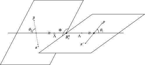
Figure 1: Angles in ${\cal D}(\vec{\Omega})$ for $B_{s}^{0}\to\Lambda(\to p\pi^{-})\overline{\Lambda}(\to\overline{p}\pi^{+})$.

When ${\bf B}_{1}$ and $\overline{{\bf B}}_{2}$ both decay subsequently, there would be three independent 3-momenta in the final states and it is possible to define an azimuthal angle. The angular distributions for $B\to{\bf B}_{1}(\to{\bf B}_{1}^{\prime}\pi)\overline{{\bf B}}_{2}(\to\overline{{\bf B}}^{\prime}_{2}\pi)$ are given as

$${\cal D}({\vec{\Omega}}) \equiv \frac{1}{\Gamma}\frac{\partial^{3}\Gamma}{\partial\Phi\partial\cos\theta_{1}\cos\theta_{2}}$$ (26)

$$= \frac{1}{8\pi}\left[1+\alpha_{1}\overline{\alpha}_{2}\cos\theta_{1}\cos\theta_{2}+\alpha(\alpha_{1}\cos\theta_{1}+\overline{\alpha}_{2}\cos\theta_{2})\right.$$

$$\left.+2\alpha_{1}\overline{\alpha}_{2}\sin\theta_{1}\sin\theta_{2}\left(\gamma\cos\Phi-\beta\sin\Phi\right)\right],\,$$

where $\theta_{1,2}$ are defined as same as the previous ones. By integrating $\theta_{1,2}$, we find

$$\frac{1}{\Gamma}\frac{\partial\Gamma}{\partial\Phi}\propto 1+\frac{\pi^{2}}{8}\alpha_{1}\alpha_{2}(\gamma\cos\Phi-\beta\sin\Phi)\,.$$ (27)

We see that $\gamma$ and $\beta$ are shown in the double cascade decays and possible to be measured in experiments. It is straightforward to see that by integrating $\phi_{1(2)}$ and $\theta_{1(2)}$, ${\cal D}(\vec{\Omega})$ reduces to ${\cal D}_{1(2)}(\theta_{1(2)})$ as expected.

IV Model calculations

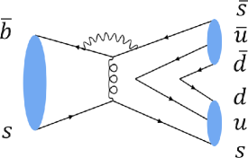
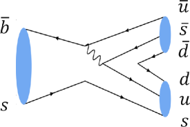
Figure 2: Quark diagrams for $B_{s}^{0}\to\Lambda\overline{\Lambda}$.

In this sections we estimate the decay parameters in the SM through model calculations. In addition to $B^{0}\to p\overline{p}$ and $B^{+}\to p\overline{\Lambda}$, we also consider the processes of $B_{s}^{0}\to\Lambda\overline{\Lambda}$ and $B_{s}^{0}\to\Sigma^{+}\overline{\Sigma}^{-}$, which are promising to be measured in the near future. The considered quark diagrams are shown in FIG. 2, where the left one is factorizable, whereas the right one is not, denoted by ${\cal A}_{P}$ and ${\cal A}_{T}$, respectively. For the $b\to f$ transition at the quark level, we have

$${\cal A}_{P}=\zeta\langle{\bf B}_{1};\overline{{\bf B}}_{2}|\overline{q}_{B}(1+\gamma_{5})f|0\rangle=\zeta\overline{u}_{1}\left(F(q^{2})+F_{5}(q^{2})\gamma_{5}\right)v_{2}\,,$$

$$\zeta=\frac{G_{F}}{\sqrt{2}}V_{tb}^{*}V_{tf}f_{B}\left(c_{6}+c_{5}/3\right)\frac{2m_{B}^{2}}{m_{b}}$$ (28)

where $q_{B}=(u,d,s)$ is the light flavor of the $B$ meson, $G_{F}$ corresponds to the Fermi constant, $V$ is the Cabibbo–Kobayashi–Maskawa matrix, $f_{B}$ ($m_{B}$) is the decay constant (mass) of $B$, $m_{b}\approx 4.5$ GeV is the $b$ quark mass, $u_{1}$ ($v_{2}$) is the Dirac spinor of ${\bf B}_{1}$ ($\overline{{\bf B}}_{2}$), and $F_{(5)}(q^{2})$ is the (pseudo)scalar form factor. In our previous work Jin:2021onb , we have used the crossing symmetry and analytical continuations to calculate $F_{(5)}(q^{2})$. It was done by assuming that the singularity does not exist in the $q^{2}$ dependence of form factors.

In this work, we adopt the ${}^{3}P_{0}$ model to calculate the form factors. The model asserts that creations of valence quarks can be approximated by scalar operators at the limit of hadrons being at rest; see Refs. Micu:1968mk ; LeYaouanc:1972vsx ; Ackleh:1996yt ; Segovia:2012cd ; Simonov:2011cm for instance. To accommodate the fact that ${\bf B}_{1}$ and $\overline{{\bf B}}_{2}$ in $B$ meson decays are far from at rest, we calculate the form factors at $\vec{v}=0$ and take their dependencies on $\vec{v}$ as  BESIII:2019hdp

$$F_{(5)}(\gamma) = \frac{{\cal F}_{(5)}}{1-5.29\gamma+7.07\gamma^{2}-0.31\gamma^{3}+0.41\gamma^{4}}\,,$$ (29)

where $\gamma=1/\sqrt{1-v^{2}}$, $\vec{v}$ is the velocity of ${\bf B}_{1}$ at the Briet frame, ${\cal F}_{(5)}$ is a constant to be fitted at $\gamma=1$ from the ${}^{3}P_{0}$ model, and the coefficients of $(5.29,7.07,-5.29,0.41)$ are extracted from the experiments of $e^{-}e^{+}\to p\overline{p}$.

The method of calculating ${\cal F}_{(5)}$ is similar to the one used in $J/\psi\to\Lambda\overline{\Sigma}^{0}$ Jpsi and we briefly quote the formalism used in the numerical evaluations here. We define the amplitudes

$$A^{{\bf B}_{1}\overline{{\bf B}}_{2}} \equiv \zeta\langle{\bf B}_{1},\uparrow;\overline{{\bf B}}_{2},\uparrow|\overline{q}_{B}f|0\rangle\,,$$

$$A^{{\bf B}_{1}\overline{{\bf B}}_{2}}_{5} \equiv \zeta\langle{\bf B}_{1},\uparrow;\overline{{\bf B}}_{2},\uparrow|\overline{q}_{B}\gamma_{5}f|0\rangle\,.$$ (30)

The factorizable parts of the helicity amplitudes are then given by $H^{fac}_{\pm}=A^{{\bf B}_{1}\overline{{\bf B}}_{2}}\pm A_{5}^{{\bf B}_{1}\overline{{\bf B}}_{2}}$. For $B^{+}\to p\overline{\Lambda}$ as an example, we find Liu:2022pdk

$$A^{p\overline{\Lambda}}_{(5)} = \gamma\zeta\gamma_{q}^{2}\frac{N^{2}}{2}\int d^{3}\vec{x}_{\Delta}\Gamma^{(5)}_{\uparrow\downarrow}\Big{[}\big{(}2E^{u}_{\uparrow\uparrow}E^{d}_{\downarrow\downarrow}+E^{u}_{\downarrow\downarrow}E^{d}_{\uparrow\uparrow}-2E^{u}_{\uparrow\downarrow}E^{d}_{\downarrow\uparrow}$$ (31)

$$-E^{u}_{\downarrow\uparrow}E^{d}_{\uparrow\downarrow}+\Gamma^{(5)}_{\uparrow\uparrow}\left(E^{u}_{\downarrow\uparrow}E^{d}_{\downarrow\downarrow}-E^{d}_{\downarrow\downarrow}E^{u}_{\downarrow\uparrow}\right)\Big{]}\,,$$

where $N$ is the normalization constant, the $\vec{x}_{\Delta}$ dependences of $E(\vec{x}_{\Delta})$ and $\Gamma(\vec{x}_{\Delta})$ have not been written out explicitly, and $\gamma_{q}\approx 0.3$ is the strength of the quark production in the $3P^{0}$ model. Here, $\Gamma_{\lambda_{1}\lambda_{2}}$ represents the overlapping of the quarks which participate in the weak interactions, whereas $E^{q}_{\lambda_{1}\lambda_{2}}$ of the spectator quark. For $\vec{v}=0$, the formalism is reduced to

$$\Gamma_{\uparrow\downarrow}(\vec{x}_{\Delta})=E_{\uparrow\downarrow}(\vec{x}_{\Delta})\,,~{}~{}~{}\Gamma_{\uparrow\uparrow}(\vec{x}_{\Delta})=E_{\uparrow\uparrow}(\vec{x}_{\Delta})\,,~{}~{}~{}\Gamma^{5}_{\uparrow\uparrow}(\vec{x}_{\Delta})=0\,,$$

$$\Gamma^{5}_{\uparrow\downarrow}(\vec{x}_{\Delta})=-2\pi\int\rho d\rho dz\left[u_{+}u_{-}+v_{+}v_{-}(\rho^{2}+z_{+}z_{-})\right]\,,$$ (32)

where the explicit forms of $N$, $E(\vec{x}_{\Delta})$, $u_{\pm}$, $v_{\pm}$ and $z_{\pm}$ and the computing techniques can be found in Ref. Jpsi . Likewise, the expressions for $B_{0}\to p\overline{p}$, $B^{0}_{s}\to\Lambda\overline{\Lambda}$ and $B^{0}_{s}\to\Sigma^{+}\overline{\Sigma}^{-}$ are

$$A^{p\overline{p}}_{(5)} = \zeta\gamma_{q}^{2}\frac{N^{2}}{2}\int d^{3}\vec{x}_{\Delta}(4E^{u}_{\downarrow\uparrow}E^{u}_{\uparrow\uparrow}\Gamma^{(5)}_{\downarrow\downarrow}+4E^{u}_{\downarrow\uparrow}E^{u}_{\downarrow\downarrow}\Gamma^{(5)}_{\uparrow\uparrow}$$

$$-4E^{u}_{\downarrow\uparrow}E^{u}_{\downarrow\uparrow}\Gamma^{(5)}_{\uparrow\downarrow}-2\Gamma^{(5)}_{\downarrow\uparrow}(E^{u}_{\downarrow\uparrow}E^{u}_{\uparrow\downarrow}+E^{u}_{\uparrow\uparrow}E^{u}_{\downarrow\downarrow}))\,,$$

$$A_{(5)}^{\Lambda\overline{\Lambda}} = \zeta\gamma_{q}^{2}\frac{N^{2}}{2}\int d^{3}\vec{x}_{\Delta}\Gamma^{(5)}_{\downarrow\uparrow}\big{(}E^{u}_{\uparrow\uparrow}E^{d}_{\downarrow\downarrow}+E^{u}_{\downarrow\downarrow}E^{d}_{\uparrow\uparrow})\,,$$

$$A_{(5)}^{\Sigma^{+}\overline{\Sigma}^{-}} = \zeta\gamma_{q}^{2}\frac{N^{2}}{2}\int d^{3}\vec{x}_{\Delta}(4E^{u}_{\downarrow\uparrow}E^{u}_{\uparrow\uparrow}\Gamma^{(5)}_{\downarrow\downarrow}+4E^{u}_{\downarrow\uparrow}E^{u}_{\downarrow\downarrow}\Gamma^{(5)}_{\uparrow\uparrow}$$ (33)

$$-4E^{u}_{\downarrow\uparrow}E^{u}_{\downarrow\uparrow}\Gamma^{(5)}_{\uparrow\downarrow}-2\Gamma^{(5)}_{\downarrow\uparrow}(E^{u}_{\downarrow\uparrow}E^{u}_{\uparrow\downarrow}+E^{u}_{\uparrow\uparrow}E^{u}_{\downarrow\downarrow}))\,.$$

We note that we have assumed the $SU(3)_{F}$ symmetry to simplify the formalism.

With the factorizable amplitudes, we find

$${\cal B}_{fac}(B^{+}\to p\overline{\Lambda})=1.57\times 10^{-7}\,,~{}~{}{\cal B}_{fac}(B_{s}^{0}\to\Lambda\overline{\Lambda})=2.6\times 10^{-7}\,,$$

$${\cal B}_{fac}(B_{s}^{0}\to\Sigma^{+}\overline{\Sigma}^{-})=2.17\times 10^{-7}\,,~{}~{}{\cal B}_{fac}(B^{0}\to p\overline{p})=0.21\times 10^{-8}\,,$$ (34)

where the subscript in ${\cal B}_{fac}$ indicates that only the factorizable part of the amplitude is considered. In Eq. (IV), ${\cal B}_{fac}(B^{+}\to p\overline{\Lambda})$ is compatible with the experimental data in Eq. (1) but ${\cal B}_{fac}(B^{0}\to p\overline{p})$ is 6 times smaller. The reason can be traced back to that ${\cal A}_{T}$ is considered yet. For $|V_{ub}^{*}V_{ud}|\gg|V_{ub}^{*}V_{us}|$ and $|V_{tb}^{*}V_{td}|\ll|V_{tb}^{*}V_{ts}|$ , ${\cal A}_{P}$ and ${\cal A}_{T}$ play a leading role in the $b\to s$ and $b\to d$ transitions, respectively.

For the nonfactorizable diagram in the right hand side of FIG. 2, we fit its amplitude from the experimental branching ratios in Eq. (1). For an estimation, we assume the relative complex phase between two diagrams to be maximum. The ratios of the nonfactorizable amplitudes among the channels are determined by the chiral selection rule described in Ref. Jin:2021onb . The ones relevant to this work read

$${\cal A}_{T}(B^{0}\to p\overline{p}):{\cal A}_{T}(B^{+}\to p\overline{\Lambda}):{\cal A}_{T}(B_{s}^{0}\to\Sigma^{+}\overline{\Sigma}^{-}):{\cal A}_{T}(B_{s}^{0}\to\Lambda\overline{\Lambda})=2:-\sqrt{6}:2:-3\,.$$ (35)

The numerical results at $t=0$ and the time-averaged ones are given in Tables 1 and 2, respectively, where ${\cal B}_{av}$ stands for the CP-even part of the branching ratio and is unaffected by the $B$ meson oscillations.

Table 1: The decay parameters at $t=0$, where the branching ratios are in units of $10^{-7}$ and the other in units of $10^{-2}$. The upper and lower columns correspond to the results with positive and negative strong phases, respectively.

channels	${\cal B}_{av}$	$A_{dir}$	$\alpha_{s}$	$\beta_{s}$	$\gamma_{s}$	$\alpha_{w}$	$\beta_{w}$	$\gamma_{w}$
$B^{0}\to p\overline{p}$	$0.127$	$29.1$	$-93.8$	$14.7$	$24.3$	$-29.1$	$-12.8$	$15.2$
	$0.127$	$-40.3$	$-93.8$	$-20.4$	$-5.3$	$40.3$	$17.8$	$-21.0$
$B^{+}\to p\overline{\Lambda}$	$2.31$	$-3.1$	$62.7$	$6.2$	$-77.3$	$3.1$	$-1.5$	$6.4$
	$2.31$	$4.2$	$59.7$	$-8.4$	$-79.3$	$-4.2$	$2.0$	$-8.7$
$B_{s}^{0}\to\Sigma^{+}\overline{\Sigma}^{-}$	$4.48$	$2.8$	$-1.1$	$-2.7$	$-99.9$	$-2.8$	$0.7$	$-2.8$
	$4.42$	$-3.9$	$0.3$	$3.9$	$-99.8$	$3.9$	$-0.9$	$3.9$
$B_{s}^{0}\to\Lambda\overline{\Lambda}$	$7.42$	$3.3$	$-1.2$	$-3.2$	$-99.9$	$-3.3$	$0.8$	$-3.3$
	$7.29$	$-4.7$	$0.5$	$4.5$	$-99.8$	$4.7$	$-1.1$	$4.7$

Table 2: The time-averaged decay parameters, where the branching ratios are in units of $10^{-7}$ and the other in units of $10^{-2}$. The upper and lower columns correspond to the results with positive and negative strong phases, respectively.

channels	${\cal B}_{av}$	$\langle A_{dir}\rangle$	$\langle\alpha_{s}\rangle$	$\langle\beta_{s}\rangle$	$\langle\gamma_{s}\rangle$	$\langle\alpha_{w}\rangle$	$\langle\beta_{w}\rangle$	$\langle\gamma_{w}\rangle$
$B^{0}\to p\overline{p}$	$0.127$	$26.2$	$-82.9$	$13.2$	$25.1$	$-29.5$	$-13.0$	$13.6$
	$0.127$	$-36.9$	$-82.8$	$-18.7$	$-5.1$	$41.7$	$18.4$	$-19.3$
$B_{s}^{0}\to\Sigma^{+}\overline{\Sigma}^{-}$	$4.48$	0.0	0.0	0.0	$-99.9$	$-2.8$	$0.7$	0.0
	$4.42$	0.0	0.0	0.0	$-99.8$	$3.9$	$-0.9$	0.0
$B_{s}^{0}\to\Lambda\overline{\Lambda}$	$7.42$	0.0	0.0	$0.0$	$-99.9$	$-2.2$	$0.5$	0.0
	$7.29$	0.0	0.0	0.0	$-99.9$	$3.1$	$-0.7$	0.0

We note there remain ambiguities in strong phases related by complex conjugates. The two possibilities would lead to an opposite sign in $A_{dir}$ and may be determined by the future experiments. In the tables, two scenarios are presented in the upper and lower columns, respectively. For the $b\to d$ transition, namely $B^{0}\to p\overline{p}$, $A_{dir}$ at $t=0$ is found to be as large as $-40.3\%$ or $29.1\%$, whereas $|A_{dir}|<7\%$ in general for the $b\to s$ transition, namely $B^{+}\to p\overline{\Lambda}$ and $B_{s}^{0}\to\Sigma^{+}\overline{\Sigma}^{-},\Lambda\overline{\Lambda}$. More importantly, due to the violent oscillation (see Eq. (22)) between $B_{s}^{0}$ and $\overline{B}_{s}^{0}$, the differences between the $B_{s}^{0}$ and $\overline{B}_{s}^{0}$ decays in the branching ratios are washed out quickly, leading to tiny $\langle A_{dir}\rangle$. In contrast, the $B^{0}$ oscillation is much more gentle, and we have $A_{dir}(t=0)\approx\langle A_{dir}\rangle$. This argument is supported by the explicit calculations as well as Eqs. (II) and (21). The same suppression due to the oscillation is found also in $\langle\gamma_{w}\rangle$ but not $\langle\alpha_{w}\rangle$ and $\langle\beta_{w}\rangle$. We conclude that $\langle\alpha_{w}\rangle$ and $\langle\beta_{w}\rangle$ are ideal observables to be probed in the experiments. In particular, $(\langle\alpha_{w}\rangle,\langle\beta_{w}\rangle)$ for $B_{s}^{0}\to\Lambda\overline{\Lambda}$ is estimated to be $(-2.2\%,0.5\%)$ or $(3.1\%,-0.7\%)$, and the relative large branching ratio of $B_{s}^{0}\to\Lambda\overline{\Lambda}$ would benefit the experimental measurement.

V conclusions

We have studied the decay observables in $B^{0}\to p\overline{p}$, $B^{+}\to p\overline{\Lambda}(\to\overline{p}\pi^{+})$, $B_{s}^{0}\to\Sigma^{+}(\to p\pi^{0})\overline{\Sigma}^{-}(\to\overline{p}\pi^{0})$ and $B_{s}^{0}\to\Lambda(\to p\pi^{-})\overline{\Lambda}(\to\overline{p}\pi^{+})$. The spin-related CP-odd and CP-even quantities in $B\to{\bf B}_{1}\overline{{\bf B}}_{2}$ have been examined. Though it is not possible to measure the spins directly at the current stage, we show that several quantities are able to be probed through the decay distributions with cascade decays. In particular, $B_{s}^{0}\to\Lambda(\to p\pi^{-})\overline{\Lambda}(\to\overline{p}\pi^{+})$ provide excellent opportunities as its final state particles are all charged.

We have estimated these quantities through the ${}^{3}P_{0}$ model and chiral selection rule within the SM. The decaying branching ratios are found to be ${\cal B}(B^{0}\to p\overline{p})=1.27\times 10^{-8}$ and ${\cal B}(B^{+}\to p\overline{\Lambda})=2.31\times 10^{-7}$, which are consistent with the current experimental data. On the other hand, ${\cal B}(B_{s}^{0}\to\Lambda\overline{\Lambda})$ is estimated to be around $7.4\times 10^{-7}$, which is about 60 times larger than ${\cal B}(B^{0}\to p\overline{p})$, making it promising to be observed in the near future. In addition, we show that $\langle A_{dir}\rangle$ are tiny for $B_{s}^{0}$ due to the violent oscillation between $B_{s}^{0}$ and $\overline{B}_{s}^{0}$.

We suggest the future experiments to visit $B_{s}^{0}\to\Lambda(\to p\pi^{-})\overline{\Lambda}(\to\overline{p}\pi^{+})$, where the time-averaged CP-odd observables are estimated to be $(\langle\alpha_{w}\rangle,\langle\beta_{w}\rangle)=(-2.2\%,0.5\%)$ or $(\langle\alpha_{w}\rangle,\langle\beta_{w}\rangle)=(3.1\%,-0.7\%)$, depending on the sign of the strong phases.

References

(1)
M. Saur and F. S. Yu,
Sci. Bull. 65, 1428 (2020);
C. Q. Geng and C. W. Liu,
JHEP 11, 104 (2021);
X. G. He, J. Tandean and G. Valencia,
Sci. Bull. 67, 1840 (2022);
X. G. He and J. P. Ma,
Phys. Lett. B 839, 137834 (2023);
Z. H. Zhang and J. J. Qi,
Eur. Phys. J. C 83, 133 (2023);
Z. H. Zhang,
Phys. Rev. D 107, L011301 (2023).
(2)
R. Aaij et al. [LHCb],
JHEP 03, 059 (2018);
R. Aaij et al. [LHCb],
JHEP 06, 084 (2018).
(3)
M. Gronau and D. London,
Phys. Lett. B 253, 483 (1991);
M. Gronau and D. Wyler,
Phys. Lett. B 265, 172 (1991);
D. Atwood, I. Dunietz and A. Soni,
Phys. Rev. Lett. 78, 3257 (1997);
D. Atwood, I. Dunietz and A. Soni,
Phys. Rev. D 63, 036005 (2001);
Y. Grossman, Z. Ligeti and A. Soffer,
Phys. Rev. D 67, 071301 (2003);
A. Giri, Y. Grossman, A. Soffer and J. Zupan,
Phys. Rev. D 68, 054018 (2003);
A. Bondar and A. Poluektov,
Eur. Phys. J. C 47, 347 (2006).
(4)
CKMfitter group, J. Charles et al.,
Phys. Rev. D 91 073007 (2015);
UTfit collaboration, M. Bona et al.,
JHEP 10, 081 (2006).
(5)
A. K. Giri, R. Mohanta and M. P. Khanna,
Phys. Rev. D 65, 073029 (2002);
S. Zhang, Y. Jiang, Z. Chen and W. Qian,
arXiv:2112.12954 [hep-ph];
C. Q. Geng, X. N. Jin, C. W. Liu, Z. Y. Wei and J. Zhang,
Phys. Lett. B 834, 137429 (2022);
S. Roy, N. G. Deshpande, A. Kundu and R. Sinha,
arXiv:2303.02591 [hep-ph].
(6)
B. Aubert et al. [BaBar], Phys. Rev. Lett. 86, 2515 (2001);
K. Abe et al. [Belle], Phys. Rev. Lett. 87, 091802 (2001).
(7)
R. L. Workman et al. [Particle Data Group],
PTEP 2022, 083C01 (2022).
(8)
R. Aaij et al. [LHCb],
JHEP 07, 041 (2014);
R. Aaij et al. [LHCb],
Phys. Rev. Lett. 116, 191601 (2016);
R. Aaij et al. [LHCb],
Phys. Rev. Lett. 122, 211803 (2019).
(9)
Z. z. Xing,
Mod. Phys. Lett. A 34, 1950238 (2019);
Y. Grossman and S. Schacht,
JHEP 07, 020 (2019);
H. Y. Cheng and C. W. Chiang,
Phys. Rev. D 100, 093002 (2019);
M. Chala, A. Lenz, A. V. Rusov and J. Scholtz,
JHEP 07, 161 (2019);
A. Dery and Y. Nir,
JHEP 12, 104 (2019);
L. Calibbi, T. Li, Y. Li and B. Zhu,
JHEP 10, 070 (2020);
H. Y. Cheng and C. W. Chiang,
Phys. Rev. D 104, 073003 (2021).
(10)
R. Aaij et al. [LHCb],
JHEP 05, 081 (2016).
(11)
C. Q. Geng, C. W. Liu and T. H. Tsai,
Phys. Lett. B 815, 136125 (2021);
J. J. Han, Y. Li, H. n. Li, Y. L. Shen, Z. J. Xiao and F. S. Yu,
Eur. Phys. J. C 82, 686 (2022);
C. W. Liu and C. Q. Geng,
JHEP 01, 128 (2022).
(12)
Private communication with Jia-Jie Han and Fu-Sheng Yu; to be appear on arXiv.
(13)
R. Aaij et al. [LHCb],
Phys. Rev. D 85, 032008 (2012);
R. Aaij et al. [LHCb],
Phys. Rev. D 99, 052006 (2019);
R. Aaij et al. [LHCb],
Phys. Rev. D 100, 031102 (2019).
(14)
C. K. Chua,
Phys. Rev. D 95, 096004 (2017);
C. K. Chua,
Phys. Rev. D 106, 036015 (2022).
(15)
R. Aaij et al. [LHCb],
JHEP 04, 162 (2017).
(16)
[LHCb],
arXiv:2206.06673 [hep-ex].
(17)
X. N. Jin, C. W. Liu and C. Q. Geng,
Phys. Rev. D 105, 053005 (2022).
(18)
H. Y. Cheng and K. C. Yang,
Phys. Rev. D 65, 054028 (2002)
[erratum: Phys. Rev. D 65, 099901 (2002)].
(19)
V. L. Chernyak and I. R. Zhitnitsky,
Nucl. Phys. B 345, 137 (1990).
(20)
H. Y. Cheng and C. K. Chua,
Phys. Rev. D 91, 036003 (2015).
(21)
C. Q. Geng and C. W. Liu,
Phys. Lett. B 825, 136883 (2022).
(22)
L. Micu,
Nucl. Phys. B 10, (1969).
(23)
A. Le Yaouanc, L. Oliver, O. Pene and J. C. Raynal,
Phys. Rev. D 8, (1973).
(24)
E. S. Ackleh, T. Barnes and E. S. Swanson,
Phys. Rev. D 54, (1996).
(25)
J. Segovia, D. R. Entem and F. Fernández,
Phys. Lett. B 715, 322 (2012).
(26)
Y. A. Simonov,
Phys. Rev. D 84, 065013 (2011).
(27)
M. Ablikim et al. [BESIII],
Phys. Rev. Lett. 124, 042001 (2020).
(28)
C. Q. Geng, C. W. Liu and J. Zhang,
arXiv:2306.02138 [hep-ph].
(29)
C. W. Liu and C. Q. Geng,
Chin. Phys. C 47, 014104 (2023).