Quasinormal Modes and Optical Properties of 4-D black holes in Einstein Power-Yang-Mills Gravity

Abstract

This paper explores the impact of the Yang-Mills charge parameter and the exponent term on a $4$D black hole solution in the Einstein Power-Yang-Mills theory. Through an investigation of the massless scalar quasinormal mode spectrum, black hole shadow, and emission rate, we have determined that the effects of these two parameters are opposite. Specifically, the Yang-Mills charge parameter causes an increase in the real quasinormal frequencies with a correspondingly smaller damping rate. It also results in a smaller black hole shadow and a lower evaporation rate.

I Introduction

Black holes, mesmerizing celestial entities subject to the principles of Einstein’s theory of gravitation, hold a prominent position in the cosmos. A groundbreaking milestone in black hole research was achieved with the detection of Gravitational Waves (GWs) on September 14th, 2015 [1]. This discovery not only advanced our understanding of black holes but also provided a novel avenue for experimentally testing theories of gravity. According to Einstein’s theory of general relativity, GWs are predicted to arise from the acceleration of massive objects, generating ripples in the fabric of spacetime. These waves carry vital information about the kinematics and dynamics of the astrophysical sources responsible for their generation. Advanced instruments such as LIGO and Virgo are capable of detecting GWs.

During the merger of two black holes, a final black hole is formed, which emits GWs exhibiting unique wave patterns known as ring-down modes. These GWs possess quasinormal modes that depend on the mass and spin of the resulting black hole. Analyzing GW data through these quasinormal modes is pivotal in unraveling the enigmatic properties of black holes and gaining valuable insights into their nature.

Quasinormal modes are a significant and intriguing characteristic of black hole physics. They are oscillations of a black hole that gradually weaken over time and are distinguished by intricate frequencies. Quasinormal modes are termed “quasinormal” because they are not precisely normal modes, which would continue to oscillate infinitely [2, 3, 4]. Rather, they fade away due to dissipative mechanisms like the emission of gravitational waves. Quasinormal modes are complex values that represent the emission of gravitational waves from compact and massive objects in the Universe. The emission frequency is denoted by the real component of the quasinormal modes, while the imaginary component corresponds to its decay. Understanding quasinormal modes is crucial because they contain information about the black hole’s characteristics, such as its mass, angular momentum, and the properties of the surrounding spacetime. Furthermore, investigating quasinormal modes provides insights into the nature of black holes and the strong gravity regime, which is challenging to explore using other methods. These modes are fundamental to understanding the structure and evolution of black holes and their role in astrophysical phenomena such as gravitational wave signals. In recent years, the exploration of GWs and the quasinormal modes exhibited by black holes has witnessed extensive investigation within various modified gravity theories [5, 6, 7, 8, 9, 10, 11, 12, 13, 14, 15, 16, 17, 18, 19].

In recent times, there has been a surge of interest in gravitational theories that incorporate the nonlinearity of Maxwell fields. The scientific community has become intrigued by the nonsingular nature of black hole solutions found in nonlinear electrodynamics [20]. Furthermore, a set of black hole solutions has been derived within the framework of power Maxwell invariant theory, where the Lagrangian density is expressed as $(\mathcal{F}_{\mu\nu}\mathcal{F}^{\mu\nu})^{q}$, with $q$ representing an arbitrary rational number [21]. Having examined black hole solutions within the context of Einstein power Maxwell invariant gravity, researchers have delved into exploring other nonlinear models that involve the coupling of nonabelian Yang-Mills fields with gravity in the realm of general relativity.

For instance, the authors in [22] investigated possible black hole solutions that are sourced by the power of Yang-Mills invariant, expressed as $(\mathcal{F}_{\alpha\beta}^{(a)}\mathcal{F}^{(a)\alpha\beta})^{q}$, where $\mathcal{F}_{\alpha\beta}^{(a)}$ is the Yang-Mills field with its internal index $1\leq a\leq{\frac{1}{2}}(D-1)(D-2)$, and setting $q=1$ recovers the $D$ dimensional Einstein-Yang-Mills black holes in $AdS$ space-time [23, 24]. Such extensions studied in the context of black hole solutions have been found to exhibit new and interesting phenomena, such as novel thermodynamic properties. Despite the complexity involved in studying these theories, they remain important areas of research for physicists interested in understanding the fundamental nature of gravity and its interaction with other forces in the Universe. Furthermore, the study of Van der Waals-like phase transitions and critical behaviour in the extended thermodynamics of $AdS$ black holes in Einstein Power-Maxwell and Einstein Power-Yang-Mills theories has been investigated [25, 26, 27, 28, 29]. Recently, the Joule-Thomson expansion for higher dimensional non-linearly charged AdS black holes in Einstein-power Maxwell invariant gravity has been explored [30]. In another study, Joule-Thomson expansion of non-linearly charged adS black holes in Einstein-power-Yang-Mills gravity has been investigated in $D$ dimensions [31]. However, the non-linearity of Yang-Mills theory naturally adds further complexity to the already non-linear nature of gravity. As a result, the theory and its associated solutions become quite intricate and difficult to analyze. This complexity presents a significant challenge for physicists trying to understand the properties and behaviour of these black holes.

The defining characteristic of a black hole is its event horizon, which is the point beyond which no particles can escape due to the immense gravitational pull. This gravitational force traps all physical particles, including light, inside the event horizon, while outside it, light can escape [32]. The matter that surrounds a black hole and is pulled inward is known as accretion. As the accretion becomes heated due to viscous dissipation, it emits bright radiation at various frequencies, including radio waves that are detectable with radio telescopes. This creates a bright background with a dark area over it, known as the black hole shadow [33]. The idea of imaging the black hole shadow at the centre of our Milky Way was first proposed by Falcke et al. [34], although the concept has been around since the 1970s. Recently, the Event Horizon Telescope captured images of the black hole shadow in the Messier 87 galaxy and Sagittarius A* [35, 36]. As a result, the black hole shadow has become a popular topic in current literature since the presence of a family of rotating black holes could provide information about the distortion of photon spheres due to the fact that rotating black holes have non-spherical horizons [37, 38, 39, 40, 41, 42, 43, 44, 45, 46, 47, 48, 49, 50, 51, 52, 53, 54, 55, 56, 57, 58, 59]. This results study of shadows in many kinds of modified gravities and also involves a comparative study with the observations of M87* and Sagittarius A* images in relation to size and shape geometric data [19, 60, 42, 61, 62, 63, 64, 65, 66, 67, 68, 69, 70]. The shadow process plays a crucial role in the discovery of the thermodynamic phase transition, which leads to a special correspondence between the two processes, from which the shadow radius is considered an efficient tool to investigate thermodynamic black hole systems [71]. Moreover, the shadow and quasi-normal modes relation is constructed in the eikonal limit, revealing that the real parts of the quasinormal modes are related to the shadow radii of black holes [72, 73].

Motivated by these studies, in this work, we intend to consider $4$-D Einstein-power-Yang-Mills gravity to investigate the quasinormal mode spectrum and optical properties of the black hole.

The paper is organised as follows. In Section II, we discuss the black hole solution in Einstein Power- Yang-Mills gravity. Section III deals with the study of quasinormal modes. In Section IV, optical behaviours of the black hole viz., shadow and emission rate have been discussed. In Section V, we discuss the connection of quasinormal modes and the optical properties in brief. Finally, in Section VI, concluding remarks are given.

Throughout the manuscript, we consider $c=\hbar=8\pi G=1$.

II 4-D Black Hole solution in Einstein Power-Yang-Mills Gravity

Initially, we begin with the $D$ dimensional action for Einstein-power-Yang-Mills gravity with non-vanishing cosmological constant given by [22]

$$I=\frac{1}{2}\int d^{D}x\sqrt{-g}\Big{(}\mathcal{R}-\frac{(D-2)(D-1)}{3}\Lambda-\mathcal{F}^{q}\Big{)},$$ (1)

where $R$ is the Ricci Scalar, $q$ is a positive real parameter and $\mathbf{F}$ is the Yang-Mills invariant, expressed as

$$\mathbf{F} = Tr(\mathcal{F}_{\lambda\sigma}^{(a)}\mathcal{F}^{(a)\lambda\sigma}),$$

$$Tr(.) = \Sigma_{a=1}^{\frac{(D-1)(D-2)}{2}}(.).$$ (2)

The Yang-Mills field is defined as [74]

$$\mathcal{F}_{\lambda\sigma}^{(a)}=\partial_{\mu}A_{\nu}^{(a)}-\partial_{\nu}A_{\mu}^{(a)}+\frac{1}{2\sigma}C_{(b)(c)}^{(a)}A_{\mu}^{(b)}A_{\mu}^{(c)}.$$ (3)

Here $C_{(b)(c)}^{(a)}$ are the structure constants of $\frac{(D-1)(D-2)}{2}$ parameter Lie group $G$ and $\sigma$ is a coupling constant, $A_{\mu}^{(a)}$ are the $SO(D-1)$ gauge group Yang-Mills potentials. We have considered the following metric ansatz for $D$ dimensions

$$ds^{2}=-f(r)dt^{2}+\frac{dr^{2}}{f(r)}+r^{2}d\Omega^{2}_{(D-2)}.$$ (4)

Here $d\Omega^{2}_{D-2}$ stands for the line element associated with unit $(D-2)$ sphere. Assuming $q\neq\frac{(D-1)}{4}$, and in the presence of cosmological constant we have the metric function of the Einstein-power-Yang-Mills black hole as given by [74]

$$f(r)=1-\frac{2M}{r^{D-3}}-\frac{\Lambda}{3}r^{2}+\frac{[(D-3)(D-2)Q^{2}]^{q}}{(D-2)(4q-D+1)r^{4q-2}}.$$ (5)

The parameter $M$ corresponds to the mass of the black hole, whereas $Q$ represents a charge parameter associated with Yang-Mills fields. For $D=4$, the metric function in Eq. (5) can be expressed in the following manner [74]:

$$f(r)=1-\frac{2M}{r}+\frac{2^{q-1}Q^{2q}r^{2-4q}}{4q-3}-\frac{\Lambda r^{2}}{3}.$$ (6)

In this study, we shall use this metric function to investigate the quasinormal modes and optical properties of the black hole. In order to satisfy the Weak Energy Condition (WEC) of the Power-Yang-Mills term, a positive value of $q$ is necessary [22]. To satisfy various energy conditions, including the causality condition, a limit for $q$ has been discussed in [22], given by $\frac{3}{4}\leq q<\frac{3}{2}$. When $q=1$, the aforementioned black hole solutions are simplified into Einstein-Yang-Mills black holes [23, 24].

III Quasinormal modes

In this section, we will address the massless scalar perturbation in the spacetime of a black hole. We will assume that the test field exerts negligible influence on the black hole spacetime. To determine the quasinormal modes, we will derive Schrödinger-like wave equations which should be of Klein-Gordon type for the case, taking into account the corresponding conservation relations of the concerned spacetime. In this study, we shall use the Padé averaged 6th order WKB approximation method, to calculate the quasinormal modes.

Considering only axial perturbation, we can express the perturbed metric as presented in [75, 13]:

$$ds^{2}= -\,|g_{tt}|\,dt^{2}+r^{2}\sin^{2}\!\theta\,(d\phi-p_{1}(t,r,\theta)\,dt$$

$$-p_{2}(t,r,\theta)\,dr-p_{3}(t,r,\theta)\,d\theta)^{2}+g_{rr}\,dr^{2}$$

$$+r^{2}d\theta^{2},$$ (7)

where the parameters $p_{1}$, $p_{2}$, and $p_{3}$ define the perturbation introduced to the black hole spacetime. The metric functions $g_{tt}$ and $g_{rr}$ represent the zeroth order terms.

III.1 Scalar Perturbation

First, we shall consider the massless scalar field near the previously established black hole. As it is considered that the effect of scalar field on the spacetime is minimal, the perturbed metric Eq. (III) can be expressed as follows:

$$ds^{2}=-\,|g_{tt}|\,dt^{2}+g_{rr}\,dr^{2}+r^{2}d\Omega^{2}.$$ (8)

Now, for this case, it’s feasible to write the Klein-Gordon equation in curved spacetime as

$$\square\Phi=\dfrac{1}{\sqrt{-g}}\partial_{\mu}(\sqrt{-g}g^{\mu\nu}\partial_{\nu}\Phi)=0.$$ (9)

With the help of this equation Eq. (9) the quasinormal modes associated with the scalar perturbation can be described. Now the scalar field can be decomposed as follows:

$$\Phi(t,r,\theta,\phi)=\dfrac{1}{r}\sum_{l,m}\psi_{l}(t,r)Y_{lm}(\theta,\phi).$$ (10)

In this equation, we have used spherical harmonics and $l$ and $m$ are the indices associated with it. Also, $\psi_{l}(t,r)$ is the radial time-dependent wave function. Using Eq. (9) and (10) one can have,

$$\partial^{2}_{r_{*}}\psi(r_{*})_{l}+\omega^{2}\psi(r_{*})_{l}=V_{s}(r)\psi(r_{*})_{l}.$$ (11)

Here in this expression, $r_{*}$ is given as

$$\dfrac{dr_{*}}{dr}=\sqrt{g_{rr}\,|g_{tt}^{-1}|}$$ (12)

and is known as the tortoise coordinate. The term $V_{s}(r)$ represents the effective potential with its explicit form as given below:

$$V_{s}(r)=|g_{tt}|\left(\dfrac{l(l+1)}{r^{2}}+\dfrac{1}{r\sqrt{|g_{tt}|g_{rr}}}\dfrac{d}{dr}\sqrt{|g_{tt}|g_{rr}^{-1}}\right),$$ (13)

here, the term $l$ represents the multipole moment of the black hole’s quasinormal modes.

Figure 1: Variation scalar potential with respect to $r$ using $M=1$, $Q=0.3$, $\Lambda=0.002$ and $q=1.1$.

Figure 2: Variation scalar potential with respect to $r$ using $M=1$ and $\Lambda=0.002$. On the first panel, we have used $Q=0.3$ and on the second $q=0.85$.

In Fig. 1 and 2, we have shown the behaviour of the scalar potential for different values of the model parameters. In Fig. 1, we show the impacts of multipole moment $l$ on the behaviour of potential. In the first panel of Fig. 2, we show the behaviour of the potential for different values of the exponent term $q$. It is seen that for the lower values of $q$, the peak value of potential increases drastically and the peak moves towards $r=0$. However, for higher values of $q$ near $1$, the variation of the potential is small and the peak also decreases slowly. The peak moves away from $r=0$ as $q$ increases. In the second panel of Fig. 2, we show how $Q$ impacts the potential of the scalar perturbation. It is seen that with an increase in the value of $Q$, the peak value of the potential increases non-linearly and the peak moves towards $r=0$. Thus the behaviour of the potential depicts that quasinormal modes might change non-linearly with respect to the model parameters $q$ and $Q$. We confirm this in the explicit calculation of quasinormal modes in the next part of our study.

III.2 The Padé averaged WKB approximation method

This investigation employed the Padé averaged sixth-order WKB approximation technique. Within this method, the oscillation frequency $\omega$ of GWs can be determined using the following expression:

$$\omega=\sqrt{-\,i\left[(n+1/2)+\sum_{k=2}^{6}\bar{\Lambda}_{k}\right]\sqrt{-2V_{0}^{\prime\prime}}+V_{0}},$$ (14)

where $n=0,1,2\ldots$, stands for overtone number, $V_{0}=V|_{r\,=\,r_{max}}$ and $V_{0}^{\prime\prime}=\dfrac{d^{2}V}{dr^{2}}|_{r\,=\,r_{max}}$. The position $r_{max}$ corresponds to the location where the potential function $V(r)$ attains its highest value. The correction terms $\bar{\Lambda}_{k}$ play a role in refining the accuracy of the calculations. The specific expressions for these correction terms, along with the Padé averaging method, can be found in the Ref.s [76, 77, 78, 79, 80]. These references provide detailed information regarding the mathematical forms of the correction terms and the procedure for Padé averaging.

Table 1: The quasinormal modes of the black hole have been computed for varying values of the multipole moment $l$ and an overtone number of $n=0$ using the 6th order Padé averaged WKB approximation method. The specific values assigned to the model parameters in this calculation are $M=1$, $Q=0.2$, $q=0.9$, and $\Lambda=0.002$.

$l$	Padé averaged WKB	$\Delta_{rms}$	$\Delta_{6}$
$1$	$0.296633\,-0.098464i$	$0.000025161$	$6.342137\times 10^{-6}$
$2$	$0.490184\,-0.0974166i$	$1.816291\times 10^{-6}$	$6.036433\times 10^{-7}$
$3$	$0.684718\,-0.0971061i$	$1.226110\times 10^{-6}$	$1.074288\times 10^{-7}$
$4$	$0.879551\,-0.0969766i$	$1.028066\times 10^{-6}$	$2.924839\times 10^{-8}$
$5$	$1.07451\,-0.0969103i$	$4.828103\times 10^{-7}$	$4.094713\times 10^{-8}$
$6$	$1.26955\,-0.0968721i$	$1.418885\times 10^{-7}$	$1.678297\times 10^{-8}$
$7$	$1.46462\,-0.096848i$	$5.412103\times 10^{-9}$	$2.204433\times 10^{-9}$
$8$	$1.65972\,-0.0968318i$	$7.714701\times 10^{-9}$	$2.274291\times 10^{-9}$

Table 1 displays the quasinormal modes for various values of the multipole moment, specifically focusing on the case where the overtone number is $n=0$. The second column of the table presents the quasinormal modes obtained through the application of the 6th-order Padé averaged WKB approximation method. Within this table, the term $\Delta_{rms}$ signifies the root mean square error associated with the 6th-order Padé averaged WKB approximation method. Furthermore, the term $\Delta_{6}$ serves as a term to quantify the error between two adjacent order approximations. It is calculated by evaluating the absolute difference between $\omega_{7}$ and $\omega_{5}$ and then dividing the result by 2, as expressed by the following equation [78]:

$$\Delta_{6}=\dfrac{|\omega_{7}-\omega_{5}|}{2}.$$ (15)

The quasinormal modes denoted as $\omega_{7}$ and $\omega_{5}$, are computed using the Padé averaged 7th order and 5th order WKB approximation methods, respectively. It is noteworthy that as the multipole moment $l$ increases, the error associated with the quasinormal modes decreases. This behaviour is a characteristic pattern of the WKB approximation method, which demonstrates limitations in providing precise results when the overtone number $n$ exceeds the multipole moment $l$[11, 12, 13, 14, 81, 15, 16].

Figure 3: Variation of real and imaginary quasinormal modes using $M=1$, $n=0$, $l=2$, $Q=0.3$ and $\Lambda=0.002$.

Figure 4: Variation of real and imaginary quasinormal modes using $M=1$, $n=0$, $l=2$, $q=1.1$ and $\Lambda=0.002$.

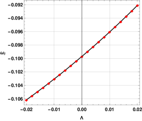
Figure 5: Variation of real and imaginary quasinormal modes using $M=1$, $n=0$, $l=2$, $q=0.9$ and $Q=0.3$.

We have shown the variation of the massless scalar quasinormal modes in Fig. 3 and 4 with respect to $q$ and $Q$, respectively. Notably, when $q=1$, the theory converges to the conventional Einstein Yang-Mills theory. For values of $q$ less than $1$, the real quasinormal frequencies and damping rate both increase drastically (see Fig. 3). Conversely, for $q>1$, the real quasinormal frequencies slowly decrease with only minor variation. At approximately $q=1.5$, the real quasinormal frequencies approach a constant value. In terms of the damping rate, we observe a decrease with a minimum decay rate occurring at $q=1.2$. As $q$ surpasses this point, the damping rate slowly begins to increase. However, the damping rate becomes almost constant as $q$ approaches $1.5$.

In Fig. 4, on the first panel, we have shown the variation of the real quasinormal frequencies with respect to the Yang-Mills charge parameter $Q$. On the second panel, we have shown the variation of the damping rate of ringdown gravitational waves with respect to $Q$. It is clearly visible that as the Yang-Mills charge parameter $Q$ increases, the real quasinormal frequencies increase exponentially. On the other hand, with an increase in the value of $Q$, the damping rate decreases exponentially. Initially, up to $Q=0.4$, the decrease in the damping rate is almost negligible. However, beyond this point, the damping rate starts to decrease drastically, reaching a minimum value at $Q=1$. Variation of quasinormal modes with respect to $\Lambda$ is shown in Fig. 5.

Hence, from the perspective of quasinormal modes, the impacts of the exponent term $q$ and the Yang-Mills charge parameter $Q$ are completely opposite. In the near future, with significant data from next-generation gravitational wave detectors like LISA, it might be possible to have a stringent bound on the Yang-Mills field with the help of quasinormal modes.

IV Optical Behaviour of the Black hole

IV.1 Shadow

This section delves into the subject of the shadow cast by black holes, which refers to the dark regions of space-time enveloping the event horizon of these astronomical phenomena. Black holes are characterized by their tremendously strong gravitational force, which is so powerful that not even light can evade its grasp once it crosses the event horizon [82, 83]. Consequently, the black hole’s periphery creates an obscure and gloomy circle against the backdrop of surrounding matter or light. The size and shape of this shadowy figure can provide critical information regarding the properties of black holes and the nature of gravity. With the aid of recent astronomical and technical advancements, it is now feasible to capture images of black hole shadows, which has significantly enhanced our understanding of these enigmatic entities [42].

We start with the Euler-Lagrange equation

$$\frac{d}{d\tau}\!\left(\frac{\partial\mathcal{L}}{\partial\dot{x}^{\mu}}\right)-\frac{\partial\mathcal{L}}{\partial x^{\mu}}=0,$$ (16)

where the Lagrangian is of the form,

$$\mathcal{L}(x,\dot{x})=\frac{1}{2}\,g_{\mu\nu}\dot{x}^{\mu}\dot{x}^{\nu}.$$ (17)

When one considers the static and spherically symmetric spacetime metric, this Lagrangian takes the form

$$\mathcal{L}(x,\dot{x})=\frac{1}{2}\left[-f(r)\,\dot{t}^{2}+\frac{1}{f(r)}\,\dot{r}^{2}+r^{2}\left(\dot{\theta}^{2}+\sin^{2}\theta\dot{\phi}^{2}\right)\right].$$ (18)

In the above expressions, the dot over the variable denotes the derivative with respect to $\tau$, the proper time.

When we opt for the equatorial plane where $\theta=\pi/2$, $\mathcal{E}$, the conserved energy and $L$, the angular momentum can be evaluated using killing vectors $\partial/\partial\tau$ and $\partial/\partial\phi$ as

$$\mathcal{E}=f(r)\,\dot{t},\quad L=r^{2}\dot{\phi}.$$ (19)

For photons, the geodesic equation can be expressed as,

$$-f(r)\,\dot{t}^{2}+\frac{\dot{r}^{2}}{f(r)}\,+r^{2}\dot{\phi}^{2}=0.$$ (20)

Using Eq. (20) together with the conserved quantities i.e.,  $\mathcal{E}$ and $L$ the orbital equation of photon can be determined as [42]

$$\left(\frac{dr}{d\phi}\right)^{2}=V_{eff},$$ (21)

here the effective potential $V_{eff}$ can be defined as

$$V_{eff}=r^{4}\left[\frac{\mathcal{E}^{2}}{L^{2}}-\frac{f(r)}{r^{2}}\right].$$ (22)

In radial form rewriting Eq. (21) will result,

$$V_{r}(r)=\dfrac{1}{\xi^{2}}-\dot{r}^{2}/L^{2}.$$ (23)

In this expression, $\xi$ is the impact parameter and can be given as $\xi=L/\mathcal{E}$. Also the reduced potential $V_{r}(r)$ can be given as

$$V_{r}(r)=\frac{f(r)}{r^{2}}.$$ (24)

In order to examine the shadow of black holes, we direct our attention to a specific point along the trajectory, denoted as $r_{ph}$. This point corresponds to the turning point, marking the location of the light ring that encircles the black hole. It can also be regarded as the radius of the photon sphere, which is of particular interest in analyzing the characteristics of the black hole’s shadow. At this turning point of a black hole, [84, 82, 85, 37, 55, 44, 42]

$$\left.V_{eff}\right|_{r_{ph}}\!\!\!\!=0,\;\;\text{and}\;\;\;\left.V_{eff}\right|_{r_{ph}}\!\!\!\!=0.$$ (25)

It is possible to obtain the impact parameter $\xi$ at the turning point as

$$\frac{1}{\xi_{crit}^{2}}=\frac{f(r_{ph})}{r_{ph}^{2}}.$$ (26)

Thus the radius of the photon sphere $r_{ph}$ can be found using [42]:

$$\left.\frac{d}{dr}\,\mathcal{A}(r)\right|_{r_{ph}}\!\!\!\!\!\!\!=0.$$ (27)

This equation can be rewritten as

$$\frac{f^{\prime}(r_{ph})}{f(r_{ph})}-\frac{h^{\prime}(r_{ph})}{h(r_{ph})}=0,$$ (28)

here $\mathcal{A}(r)=h(r)/f(r)$ with $h(r)=r^{2}$.

Now, in order to obtain the shadow of the black hole, we rewrite Eq. (21) with Eq. (26), in terms of the function $\mathcal{A}(r)$ as

$$\left(\frac{dr}{d\phi}\right)^{\!2}=h(r)f(r)\left(\frac{\mathcal{A}(r)}{\mathcal{A}(r_{ph})}-1\right).$$ (29)

Using this Eq. (29), one can obtain the shadow radius of the black hole. When examining the scenario where a static observer is located at a distance $r_{0}$ from the black hole, we can determine the angle $\alpha$ between the light rays emanating from the observer and the radial direction of the photon sphere. This angle can be calculated as [42]

$$\cot\alpha=\frac{1}{\sqrt{f(r)h(r)}}\left.\frac{dr}{d\phi}\right|_{r\,=\,r_{0}}\!\!\!\!\!\!\!\!\!\!\!.$$ (30)

Together with Eq. (29), we can express the above equation as

$$\cot^{2}\!\alpha=\frac{\mathcal{A}(r_{0})}{\mathcal{A}(r_{ph})}-1.$$ (31)

Again, above equation can be rewritten using the relation $\sin^{2}\!\alpha=1/(1+\cot^{2}\!\alpha)$ as

$$\sin^{2}\!\alpha=\frac{\mathcal{A}(r_{ph})}{\mathcal{A}(r_{0})}.$$ (32)

Substitution of the form of $\mathcal{A}(r_{ph})$ from Eq. (26) and $\mathcal{A}(r_{0})=r_{0}^{2}/f(r_{0})$ the black hole’s shadow radius for a static observer at $r_{0}$ is estimated as [42]

$$R_{s}=r_{0}\sin\alpha=\sqrt{\frac{r_{ph}^{2}f(r_{0})}{f\left(r_{ph}\right)}}.$$ (33)

Again, for asymptotically flat spacetime at $r_{0}\rightarrow\infty$ i.e. for a static observer at large distance, $f(r_{0})\rightarrow 1$, so for such an observer the shadow radius $R_{s}$ becomes,

$$R_{s}=\frac{r_{ph}}{\sqrt{f(r_{ph})}}.$$ (34)

But in this scenario, the black hole spacetime is not asymptotically flat for $\Lambda\neq 0$. Hence, the black hole shadow will have an observer distance dependency. In this case, one should note that for dS spacetime, the black hole can have two horizons viz., event horizon and cosmological horizon. Any physical observer is expected to lie in between these two horizons.

Finally, via the stereographic projection of the shadow from the black hole’s plane to the observer’s image plane with coordinates $(X,Y)$, the apparent form of the shadow can be determined. These coordinates are defined as [42, 86, 10]

$$X =-\,r_{0}^{2}\sin\theta_{0}\left.\frac{d\phi}{dr}\right|_{r_{0}},$$ (35)

$$Y =r_{0}^{2}\left.\frac{d\theta}{dr}\right|_{(r_{0},\theta_{0})},$$ (36)

here $\theta_{0}$ represents the angular position of the observer with respect to the plane of the black hole.

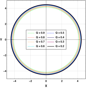
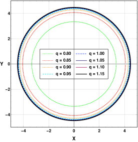
Figure 6: Stereographic projection of black hole shadow using observer distance $r_{0}=10,$ $M=1$ and $\Lambda=0.002$. On the first panel, we have used $Q=0.3$ and on the second panel $q=1.1$.

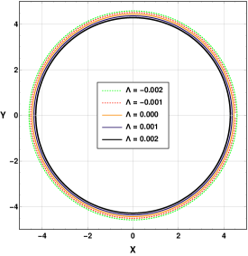
Figure 7: Stereographic projection of black hole shadow using observer distance $r_{0}=10,$ $M=1$, $Q=0.3$ and $q=0.9$.

The investigation presents the stereographic projections of the black hole’s shadow, offering visual representations that depict the shadow’s characteristics for the specific black hole being examined. Fig. 6 showcases these projections, providing insights into the shadow’s behaviour across various model parameters. In the initial panel of Fig. 6, the stereographic projections illustrate the black hole’s shadow for different values of the model parameter $Q$. Remarkably, as the model parameter $Q$ increases, a discernible reduction in the black hole’s shadow is observed.

Moving to the second panel, we observe the shadow of the black hole for different values of the parameter $q$. It becomes evident that an increase in the parameter $q$ leads to a nonlinear growth in the black hole’s shadow. Particularly noteworthy is the significant impact of small variations in $q$ around the value of $0.80$, resulting in a substantial alteration in the black hole’s shadow. However, as $q$ approaches larger values near $1$, the effect on the black hole’s shadow becomes increasingly marginal. Thus, this investigation demonstrates that both model parameters exert distinct influences on the black hole’s shadow.

Finally, in Fig. 7, we have shown the effect of the cosmological constant $\Lambda$ on the black hole shadow. One can see that for the dS black hole shadow is of smaller size while for the AdS case, the black hole shadow is comparatively larger.

IV.2 Emission rate

Through the examination of the black hole shadow, it is possible to investigate the emission of particles in the vicinity of the black hole. Studies have demonstrated that, for an observer positioned far away, the black hole shadow is an indication of the black hole’s high-energy absorption cross-section [87]. Generally speaking, when dealing with a spherically symmetric black hole, the absorption cross-section shows oscillatory behaviour around a constant limiting value of $\sigma_{lim}$ at extremely high energies. Since the shadow provides a way to visually detect a black hole, it is roughly equivalent to the area of the photon sphere, which can be estimated as $\sigma_{lim}\approx\pi R_{s}^{2}$. The energy emission rate can be calculated using the following expression [87, 82, 88, 89]:

$$\frac{d^{2}\mathcal{E}(\omega)}{dtd\omega}=\frac{2\pi^{3}\omega^{3}R_{s}^{2}}{e^{\frac{\omega}{T}}-1},$$ (37)

in which $\omega$ is the emission frequency, and $T$ is the Hawking temperature given by

$$T=\dfrac{f^{\prime}(r_{h})}{4\pi},$$ (38)

where $r_{h}$ represents the event horizon of the black hole.

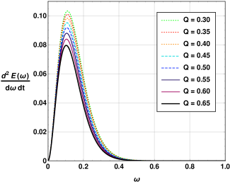
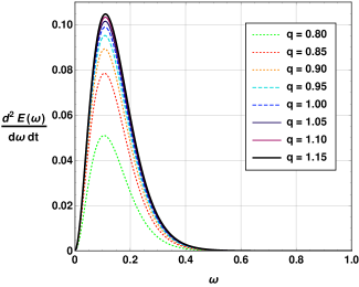
Figure 8: Emission rate of the black hole with respect to $\omega$ using observer distance $r_{0}=10,$ $M=1$ and $\Lambda=0.002$. On the first panel, we have used $q=1.1$ and on the second panel $Q=0.3$.

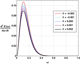
Figure 9: Emission rate of the black hole with respect to $\omega$ using observer distance $r_{0}=10,$ $M=1$, $Q=0.3$ and $q=0.9$.

By utilizing the Hawking temperature expression provided in Eq. (37), we have illustrated the change in emission rate concerning $\omega$ for various values of $Q$ (displayed on the first panel) and $q$ (shown on the second panel) in Fig. 8. It is noticeable that as the parameter $Q$ increases, the emission rate of the black hole reduces. In contrast, with an increase in the parameter $q$, the emission rate of the black hole increases slowly. Therefore, the examination indicates that as the Yang-Mills charge parameter $Q$ grows, the black hole’s evaporation rate decreases, and its lifespan extends. Conversely, as the parameter $q$ increases, the black hole’s evaporation rate gradually increases, and its lifespan shortens.

In Fig. 9, we have shown the impacts on the emission rate by the cosmological constant $\Lambda$. One can see that for the AdS case, emission rate is higher resulting short lifespan of the black hole while in the case of dS scenario, the emission rate decreases resulting a black hole with a longer lifespan.

V Connection between quasinormal modes and optical properties of the black hole

The shadow of the black hole is associated with the quasinormal modes. An investigation of their connection can be helpful to make predictions of the quasinormal mode behaviours from the observational results of black hole shadow. Moreover, it also can help us to put a constraint on the quasinormal modes from the black hole shadow observations. To obtain an approximate relation of the black hole shadow with quasinormal modes, we can use the WKB formula. However, higher-order WKB formula can result in a more complicated relation. In this study, we are primarily interested to see how they are related in the eikonal regime. Hence, although we have used 6th-order WKB approximations in the previous part of the investigation, here we can simply use 3rd-order WKB approximation, as both formulas will give us the same leading order approximations in the eikonal regime.

At first, we start with the expression of the third-order WKB expansion of quasinormal mode frequency as follows [90, 91]:

$$\omega=\Bigg{\{}V+\frac{V_{4}}{8V_{2}}\left(\nu^{2}+\frac{1}{4}\right)-\left(\frac{7+60\nu^{2}}{288}\right)\frac{V_{3}^{2}}{V_{2}^{2}}+i\nu\sqrt{-2V_{2}}\left[\frac{1}{2V_{2}}\left[\frac{5V_{3}^{4}(77+188\nu^{2})}{6912V_{2}^{4}}\right.\right.$$

$$\left.\left.-\frac{V_{3}^{2}V_{4}(51+100\nu^{2})}{384V_{2}^{3}}+\frac{V_{4}^{2}(67+68\nu^{2})}{2304V_{2}^{2}}+\frac{V_{5}V_{3}(19+28\nu^{2})}{288V_{2}^{2}}+\frac{V_{6}(5+4\nu^{2})}{288V_{2}}\right]-1\right]\Bigg{\}}^{1/2}_{r=r_{ph}}.$$

(39)

In this context, $V_{i}$ denotes the derivative of the potential $V$ with respect to its $i$-th variable. Furthermore, $\nu$ is defined as the overtone number, represented by $n+1/2$, where $n$ is a natural number. The expression for the frequency $\omega$ mentioned above should be evaluated at the specific point $r_{ph}$, which is defined as the maximum value attained by the potential $V$ throughout the system. One may note that this relation can provide the quasinormal modes up to a satisfactory accuracy. However, this formula can result in larger errors when the overtone number $n$ is greater than the multipole number $l$. The error decreases significantly when $l>>n$.

Eventually, when we expand Eq. (39), we acquire, specifically in the eikonal regime [91],

$$\omega=\left[(2\ell+1)\frac{\sqrt{f(r)}}{2r}+\mathcal{O}(\ell^{-1})\right]_{r=r_{ph}}-i\left[\frac{n+1/2}{\sqrt{2}}\frac{\sqrt{f(r)}}{r}\sqrt{6rf^{\prime}(r)-6f(r)-r^{2}f^{\prime\prime}(r)-r^{2}f(r)^{-1}{f^{\prime}(r)}^{2}}+\mathcal{O}(\ell^{-1})\right]_{r=r_{ph}}.$$

The leading-order approximation of the imaginary part can be expressed as follows [91]:

$$\omega_{I}=\frac{n+1}{\sqrt{2}}R_{s}^{-1}\sqrt{2f(r_{ph})-r_{ph}^{2}f^{\prime\prime}(r_{ph})}+\mathcal{O}(\ell^{-1}).$$ (40)

Regarding the real part, in the leading order approximation, it precisely corresponds to the shadow radius of the black hole. However, in the sub-leading regime, it is equal to half of the shadow radius’s value. The leading-order approximations provide [91]

$$\omega_{R}=R_{s}^{-1}\left(\ell+\frac{1}{2}+\mathcal{O}(\ell^{-1})\right).$$ (41)

From Eq.s 40 and 41, one can see that at the eikonal regime, the shadow radius of the black hole is inversely connected with the damping rate and GW oscillation frequency. Hence, at the eikonal limit, it is possible to constrain the damping rate and the GW oscillation frequency with the help of black hole shadow. We leave it as a future prospect of this work. Moreover, Eq. (37) shows that the emission rate is associated with the square of the black hole shadow radius, hence, knowing the Hawking temperature, it is possible to comment on the emission rate from the quasinormal modes. In the near future, from significant observational results from LISA, one might be able to have a strong constraint on the quasinormal modes which will also shed some light on the emission rate of the black hole as well as the stability.

VI Concluding Remarks

Our investigation has unveiled that the Yang-Mills charge parameter, denoted as $Q$, and the exponent term, denoted as $q$, exert substantial influences on the quasinormal spectrum and optical characteristics of a four-dimensional black hole governed by Einstein Power-Yang-Mills gravity. Remarkably, these two parameters exhibit diametrically opposite effects on the quasinormal mode spectrum.

To gain a clearer understanding of the behaviour of these Yang-Mills field parameters, we have examined the black hole’s shadow and emission rate. Our findings indicate that the black hole’s shadow size decreases as the Yang-Mills charge parameter $Q$ increases. Conversely, the exponent parameter $q$ shows contrasting behaviour, as an increase in its value leads to an augmented shadow. This variation is particularly prominent when $q$ approaches its lower boundary of 0.75. Additionally, we have analyzed the black hole’s emission rate. As the Yang-Mills charge parameter $Q$ rises, the black hole’s evaporation rate decreases. On the other hand, an increase in the value of $q$ increases the evaporation rate, indicating a reduced lifespan for the black hole.

Therefore, our research underscores the significant impact of both the Yang-Mills charge parameter and the exponent term on the quasinormal spectrum and optical properties of a four-dimensional black hole governed by Einstein Power-Yang-Mills gravity.

References

- Abbott et al. [2016] B. P. Abbott et al. (LIGO Scientific Collaboration and Virgo Collaboration), “Observation of gravitational waves from a binary black hole merger,” Phys. Rev. Lett. 116, 061102 (2016).
- Vishveshwara [1970] C. V. Vishveshwara, “Scattering of Gravitational Radiation by a Schwarzschild Black-hole,” Nature 227, 936 (1970).
- Press [1971] W. H. Press, “Long Wave Trains of Gravitational Waves from a Vibrating Black Hole,” Astrophys. J. Lett. 170, L105 (1971).
- Kokkotas and Schmidt [1999] K. D. Kokkotas and B. G. Schmidt, “Quasinormal modes of stars and black holes,” Living Rev. Rel. 2, 2 (1999), arXiv:gr-qc/9909058.
- Rincón and Panotopoulos [2018] A. Rincón and G. Panotopoulos, “Greybody factors and quasinormal modes for a nonminimally coupled scalar field in a cloud of strings in (2+1)-dimensional background,” Eur. Phys. J. C 78, 858 (2018), arXiv:1810.08822 [gr-qc].
- Liu et al. [2022] D. Liu, Y. Yang, A. Övgün, Z.-W. Long, and Z. Xu, “Quasinormal Modes and Greybody Bounds of Rotating Black Holes in a Dark Matter Halo,” (2022), arXiv:2204.11563 [gr-qc].
- Rincon et al. [2022] A. Rincon, P. A. Gonzalez, G. Panotopoulos, J. Saavedra, and Y. Vasquez, “Quasinormal modes for a non-minimally coupled scalar field in a five-dimensional Einstein–Power–Maxwell background,” Eur. Phys. J. Plus 137, 1278 (2022), arXiv:2112.04793 [gr-qc].
- Ovgün and Jusufi [2018] A. Ovgün and K. Jusufi, “Quasinormal Modes and Greybody Factors of gravity minimally coupled to a cloud of strings in Dimensions,” Annals Phys. 395, 138 (2018), arXiv:1801.02555 [gr-qc].
- Övgün et al. [2021] A. Övgün, I. Sakallı, and H. Mutuk, “Quasinormal modes of dS and AdS black holes: Feedforward neural network method,” Int. J. Geom. Meth. Mod. Phys. 18, 2150154 (2021), arXiv:1904.09509 [gr-qc].
- Anacleto et al. [2021] M. A. Anacleto, J. A. V. Campos, F. A. Brito, and E. Passos, “Quasinormal modes and shadow of a Schwarzschild black hole with GUP,” Annals Phys. 434, 168662 (2021), arXiv:2108.04998 [gr-qc].
- Lambiase et al. [2023] G. Lambiase, R. C. Pantig, D. J. Gogoi, and A. Övgün, “Investigating the Connection between Generalized Uncertainty Principle and Asymptotically Safe Gravity in Black Hole Signatures through Shadow and Quasinormal Modes,” (2023), arXiv:2304.00183 [gr-qc].
- Sekhmani and Gogoi [2023] Y. Sekhmani and D. J. Gogoi, “Electromagnetic quasinormal modes of dyonic AdS black holes with quasitopological electromagnetism in a Horndeski gravity theory mimicking EGB gravity at D → 4,” International Journal of Geometric Methods in Modern Physics , 2350160 (2023).
- Gogoi et al. [2023a] D. J. Gogoi, A. Övgün, and M. Koussour, “Quasinormal Modes of Black holes in gravity,” (2023a), arXiv:2303.07424 [gr-qc].
- Parbin et al. [2022] N. Parbin, D. J. Gogoi, J. Bora, and U. D. Goswami, “Deflection angle and quasinormal modes of a de Sitter black hole in gravity,” (2022), arXiv:2211.02414 [gr-qc].
- Karmakar et al. [2022] R. Karmakar, D. J. Gogoi, and U. D. Goswami, “Quasinormal modes and thermodynamic properties of GUP-corrected Schwarzschild black hole surrounded by quintessence,” International Journal of Modern Physics A 37, 2250180 (2022).
- Gogoi and Goswami [2022] D. J. Gogoi and U. D. Goswami, “Quasinormal modes and Hawking radiation sparsity of GUP corrected black holes in bumblebee gravity with topological defects,” JCAP 06, 029 (2022), arXiv:2203.07594 [gr-qc].
- Gogoi et al. [2023b] D. J. Gogoi, R. Karmakar, and U. D. Goswami, “Quasinormal modes of nonlinearly charged black holes surrounded by a cloud of strings in Rastall gravity,” Int. J. Geom. Meth. Mod. Phys. 20, 2350007 (2023b), arXiv:2111.00854 [gr-qc].
- Gogoi and Goswami [2021] D. J. Gogoi and U. D. Goswami, “Quasinormal modes of black holes with non-linear-electrodynamic sources in Rastall gravity,” Phys. Dark Univ. 33, 100860 (2021), arXiv:2104.13115 [gr-qc].
- Pantig et al. [2022a] R. C. Pantig, L. Mastrototaro, G. Lambiase, and A. Övgün, “Shadow, lensing, quasinormal modes, greybody bounds and neutrino propagation by dyonic ModMax black holes,” Eur. Phys. J. C 82, 1155 (2022a), arXiv:2208.06664 [gr-qc].
- Ayon-Beato and Garcia [1998] E. Ayon-Beato and A. Garcia, “Regular black hole in general relativity coupled to nonlinear electrodynamics,” Phys. Rev. Lett. 80, 5056 (1998), arXiv:gr-qc/9911046.
- Maeda et al. [2009] H. Maeda, M. Hassaine, and C. Martinez, “Lovelock black holes with a nonlinear Maxwell field,” Phys. Rev. D 79, 044012 (2009), arXiv:0812.2038 [gr-qc].
- Mazharimousavi and Halilsoy [2009] S. H. Mazharimousavi and M. Halilsoy, “Lovelock black holes with a power-Yang-Mills source,” Phys. Lett. B 681, 190 (2009), arXiv:0908.0308 [gr-qc].
- Habib Mazharimousavi and Halilsoy [2007] S. Habib Mazharimousavi and M. Halilsoy, “5D black hole solution in Einstein-Yang-Mills-Gauss-Bonnet theory,” Phys. Rev. D 76, 087501 (2007), arXiv:0801.1562 [gr-qc].
- Mazharimousavi and Halilsoy [2008] S. H. Mazharimousavi and M. Halilsoy, “Einstein-Yang-Mills black hole solution in higher dimensions by the Wu-Yang Ansatz,” Phys. Lett. B 659, 471 (2008), arXiv:0801.1554 [gr-qc].
- Hendi et al. [2018] S. H. Hendi, B. E. Panah, and S. Panahiyan, “Black Hole Solutions in Gauss-Bonnet-Massive Gravity in the Presence of Power-Maxwell Field,” Fortsch. Phys. 66, 1800005 (2018), arXiv:1708.02239 [hep-th].
- Zhang et al. [2015] M. Zhang, Z.-Y. Yang, D.-C. Zou, W. Xu, and R.-H. Yue, “ criticality of AdS black hole in the Einstein-Maxwell-power-Yang-Mills gravity,” Gen. Rel. Grav. 47, 14 (2015), arXiv:1412.1197 [hep-th].
- Yerra and Chandrasekhar [2019] P. K. Yerra and B. Chandrasekhar, “Heat engines at criticality for nonlinearly charged black holes,” Mod. Phys. Lett. A 34, 1950216 (2019), arXiv:1806.08226 [hep-th].
- Hendi et al. [2017a] S. H. Hendi, B. Eslam Panah, S. Panahiyan, and A. Sheykhi, “Dilatonic BTZ black holes with power-law field,” Phys. Lett. B 767, 214 (2017a), arXiv:1703.03403 [gr-qc].
- Hendi et al. [2017b] S. H. Hendi, B. Eslam Panah, S. Panahiyan, and M. S. Talezadeh, “Geometrical thermodynamics and P-V criticality of black holes with power-law Maxwell field,” Eur. Phys. J. C 77, 133 (2017b), arXiv:1612.00721 [hep-th].
- Feng et al. [2021] Z.-W. Feng, X. Zhou, G. He, S.-Q. Zhou, and S.-Z. Yang, “Joule–Thomson expansion of higher dimensional nonlinearly AdS black hole with power Maxwell invariant source,” Commun. Theor. Phys. 73, 065401 (2021), arXiv:2009.02172 [gr-qc].
- Biswas [2021] A. Biswas, “Joule-Thomson expansion of AdS black holes in Einstein Power-Yang-mills gravity,” Phys. Scripta 96, 125310 (2021), arXiv:2106.11066 [gr-qc].
- Synge [1966] J. L. Synge, “The Escape of Photons from Gravitationally Intense Stars,” Mon. Not. Roy. Astron. Soc. 131, 463 (1966).
- Luminet [1979] J. P. Luminet, “Image of a spherical black hole with thin accretion disk,” Astron. Astrophys. 75, 228 (1979).
- Falcke et al. [2000] H. Falcke, F. Melia, and E. Agol, “Viewing the shadow of the black hole at the galactic center,” Astrophys. J. Lett. 528, L13 (2000), arXiv:astro-ph/9912263.
- Akiyama et al. [2019] K. Akiyama et al. (Event Horizon Telescope), “First M87 Event Horizon Telescope Results. I. The Shadow of the Supermassive Black Hole,” Astrophys. J. Lett. 875, L1 (2019), arXiv:1906.11238 [astro-ph.GA].
- Akiyama et al. [2022] K. Akiyama et al. (Event Horizon Telescope), “First Sagittarius A* Event Horizon Telescope Results. I. The Shadow of the Supermassive Black Hole in the Center of the Milky Way,” Astrophys. J. Lett. 930, L12 (2022).
- Övgün et al. [2018] A. Övgün, I. Sakallı, and J. Saavedra, “Shadow cast and Deflection angle of Kerr-Newman-Kasuya spacetime,” JCAP 10, 041 (2018), arXiv:1807.00388 [gr-qc].
- Kocherlakota et al. [2021] P. Kocherlakota et al. (Event Horizon Telescope), “Constraints on black-hole charges with the 2017 EHT observations of M87*,” Phys. Rev. D 103, 104047 (2021), arXiv:2105.09343 [gr-qc].
- Belhaj et al. [2021] A. Belhaj, H. Belmahi, M. Benali, W. El Hadri, H. El Moumni, and E. Torrente-Lujan, “Shadows of 5D black holes from string theory,” Phys. Lett. B 812, 136025 (2021), arXiv:2008.13478 [hep-th].
- Belhaj et al. [2020] A. Belhaj, M. Benali, A. El Balali, H. El Moumni, and S. E. Ennadifi, “Deflection angle and shadow behaviors of quintessential black holes in arbitrary dimensions,” Class. Quant. Grav. 37, 215004 (2020), arXiv:2006.01078 [gr-qc].
- Belhaj and Sekhmani [2022] A. Belhaj and Y. Sekhmani, “Shadows of rotating quintessential black holes in Einstein–Gauss–Bonnet gravity with a cloud of strings,” Gen. Rel. Grav. 54, 17 (2022).
- Gogoi et al. [2023c] D. J. Gogoi, Y. Sekhmani, D. Kalita, N. J. Gogoi, and J. Bora, “Joule‐Thomson Expansion and Optical Behaviour of Reissner‐Nordström‐Anti‐de Sitter Black Holes in Rastall Gravity Surrounded by a Quintessence Field,” Fortschritte der Physik 71, 2300010 (2023c).
- Övgün and Sakallı [2020] A. Övgün and I. Sakallı, “Testing generalized Einstein–Cartan–Kibble–Sciama gravity using weak deflection angle and shadow cast,” Class. Quant. Grav. 37, 225003 (2020), arXiv:2005.00982 [gr-qc].
- Övgün et al. [2020] A. Övgün, I. Sakallı, J. Saavedra, and C. Leiva, “Shadow cast of noncommutative black holes in Rastall gravity,” Mod. Phys. Lett. A 35, 2050163 (2020), arXiv:1906.05954 [hep-th].
- Kuang and Övgün [2022] X.-M. Kuang and A. Övgün, “Strong gravitational lensing and shadow constraint from M87* of slowly rotating Kerr-like black hole,” (2022), arXiv:2205.11003 [gr-qc].
- Kumaran and Övgün [2022] Y. Kumaran and A. Övgün, “Deflection Angle and Shadow of the Reissner–Nordström Black Hole with Higher-Order Magnetic Correction in Einstein-Nonlinear-Maxwell Fields,” Symmetry 14, 2054 (2022), arXiv:2210.00468 [gr-qc].
- Mustafa et al. [2022] G. Mustafa, F. Atamurotov, I. Hussain, S. Shaymatov, and A. Övgün, “Shadows and gravitational weak lensing by the Schwarzschild black hole in the string cloud background with quintessential field*,” Chin. Phys. C 46, 125107 (2022), arXiv:2207.07608 [gr-qc].
- Cimdiker et al. [2021] I. Cimdiker, D. Demir, and A. Övgün, “Black hole shadow in symmergent gravity,” Phys. Dark Univ. 34, 100900 (2021), arXiv:2110.11904 [gr-qc].
- Okyay and Övgün [2022] M. Okyay and A. Övgün, “Nonlinear electrodynamics effects on the black hole shadow, deflection angle, quasinormal modes and greybody factors,” JCAP 01, 009 (2022), arXiv:2108.07766 [gr-qc].
- Atamurotov et al. [2023] F. Atamurotov, I. Hussain, G. Mustafa, and A. Övgün, “Weak deflection angle and shadow cast by the charged-Kiselev black hole with cloud of strings in plasma*,” Chin. Phys. C 47, 025102 (2023).
- Pantig et al. [2023] R. C. Pantig, A. Övgün, and D. Demir, “Testing symmergent gravity through the shadow image and weak field photon deflection by a rotating black hole using the M87$$^*$$ and Sgr. $$\hbox {A}^*$$ results,” The European Physical Journal C 83, 250 (2023).
- Abdikamalov et al. [2019] A. B. Abdikamalov, A. A. Abdujabbarov, D. Ayzenberg, D. Malafarina, C. Bambi, and B. Ahmedov, “Black hole mimicker hiding in the shadow: Optical properties of the metric,” Phys. Rev. D 100, 024014 (2019), arXiv:1904.06207 [gr-qc].
- Abdujabbarov et al. [2016] A. Abdujabbarov, B. Juraev, B. Ahmedov, and Z. Stuchlik, “Shadow of rotating wormhole in plasma environment,” Astrophys. Space Sci. 361, 226 (2016).
- Atamurotov and Ahmedov [2015] F. Atamurotov and B. Ahmedov, “Optical properties of black hole in the presence of plasma: shadow,” Phys. Rev. D 92, 084005 (2015), arXiv:1507.08131 [gr-qc].
- Papnoi et al. [2014] U. Papnoi, F. Atamurotov, S. G. Ghosh, and B. Ahmedov, “Shadow of five-dimensional rotating Myers-Perry black hole,” Phys. Rev. D 90, 024073 (2014), arXiv:1407.0834 [gr-qc].
- Abdujabbarov et al. [2013] A. Abdujabbarov, F. Atamurotov, Y. Kucukakca, B. Ahmedov, and U. Camci, “Shadow of Kerr-Taub-NUT black hole,” Astrophys. Space Sci. 344, 429 (2013), arXiv:1212.4949 [physics.gen-ph].
- Atamurotov et al. [2013] F. Atamurotov, A. Abdujabbarov, and B. Ahmedov, “Shadow of rotating non-Kerr black hole,” Phys. Rev. D 88, 064004 (2013).
- Cunha and Herdeiro [2018] P. V. P. Cunha and C. A. R. Herdeiro, “Shadows and strong gravitational lensing: a brief review,” Gen. Rel. Grav. 50, 42 (2018), arXiv:1801.00860 [gr-qc].
- Gralla et al. [2019] S. E. Gralla, D. E. Holz, and R. M. Wald, “Black Hole Shadows, Photon Rings, and Lensing Rings,” Phys. Rev. D 100, 024018 (2019), arXiv:1906.00873 [astro-ph.HE].
- Lobos and Pantig [2022] N. J. L. S. Lobos and R. C. Pantig, “Generalized extended uncertainty principle black holes: Shadow and lensing in the macro- and microscopic realms,” Physics 4, 1318 (2022).
- Uniyal et al. [2023] A. Uniyal, S. Chakrabarti, R. C. Pantig, and A. Övgün, “Nonlinearly charged black holes: Shadow and Thin-accretion disk,” (2023), arXiv:2303.07174 [gr-qc].
- Panotopoulos et al. [2021] G. Panotopoulos, A. Rincón, and I. Lopes, “Orbits of light rays in scale-dependent gravity: Exact analytical solutions to the null geodesic equations,” Phys. Rev. D 103, 104040 (2021), arXiv:2104.13611 [gr-qc].
- Panotopoulos and Rincon [2022] G. Panotopoulos and A. Rincon, “Orbits of light rays in -dimensional Einstein–power–Maxwell gravity: Exact analytical solution to the null geodesic equations,” Annals Phys. 443, 168947 (2022), arXiv:2206.03437 [gr-qc].
- Khodadi and Lambiase [2022] M. Khodadi and G. Lambiase, “Probing Lorentz symmetry violation using the first image of Sagittarius A*: Constraints on standard-model extension coefficients,” Phys. Rev. D 106, 104050 (2022), arXiv:2206.08601 [gr-qc].
- Khodadi et al. [2021] M. Khodadi, G. Lambiase, and D. F. Mota, “No-hair theorem in the wake of Event Horizon Telescope,” JCAP 09, 028 (2021), arXiv:2107.00834 [gr-qc].
- Zhao et al. [2023] Y. Zhao, Y. Cai, S. Das, G. Lambiase, E. N. Saridakis, and E. C. Vagenas, “Quasinormal Modes in Noncommutative Schwarzschild black holes,” (2023), arXiv:2301.09147 [gr-qc].
- Khodadi et al. [2020] M. Khodadi, A. Allahyari, S. Vagnozzi, and D. F. Mota, “Black holes with scalar hair in light of the Event Horizon Telescope,” JCAP 09, 026 (2020), arXiv:2005.05992 [gr-qc].
- Khodadi and Saridakis [2021] M. Khodadi and E. N. Saridakis, “Einstein-Æther gravity in the light of event horizon telescope observations of M87*,” Phys. Dark Univ. 32, 100835 (2021), arXiv:2012.05186 [gr-qc].
- Vagnozzi et al. [2023] S. Vagnozzi et al., “Horizon-scale tests of gravity theories and fundamental physics from the Event Horizon Telescope image of Sagittarius A,” Class. Quant. Grav. 40, 165007 (2023), arXiv:2205.07787 [gr-qc].
- Khodadi [2022] M. Khodadi, “Shadow of black hole surrounded by magnetized plasma: Axion-plasmon cloud,” Nucl. Phys. B 985, 116014 (2022), arXiv:2211.00300 [gr-qc].
- Zhang and Guo [2020] M. Zhang and M. Guo, “Can shadows reflect phase structures of black holes?” Eur. Phys. J. C 80, 790 (2020), arXiv:1909.07033 [gr-qc].
- Jusufi [2020] K. Jusufi, “Connection Between the Shadow Radius and Quasinormal Modes in Rotating Spacetimes,” Phys. Rev. D 101, 124063 (2020), arXiv:2004.04664 [gr-qc].
- Jusufi [2021] K. Jusufi, “Correspondence between quasinormal modes and the shadow radius in a wormhole spacetime,” Gen. Rel. Grav. 53, 87 (2021), arXiv:2007.16019 [gr-qc].
- Biswas [2022] A. Biswas, “Black holes in 4D AdS Einstein Gauss Bonnet gravity with power: Yang Mills field,” Gen. Rel. Grav. 54, 161 (2022), arXiv:2208.02290 [gr-qc].
- Bouhmadi-López et al. [2020] M. Bouhmadi-López, S. Brahma, C.-Y. Chen, P. Chen, and D.-h. Yeom, “A consistent model of non-singular Schwarzschild black hole in loop quantum gravity and its quasinormal modes,” JCAP 07, 066 (2020), arXiv:2004.13061 [gr-qc].
- Schutz and Will [1985] B. F. Schutz and C. M. Will, “BLACK HOLE NORMAL MODES: A SEMIANALYTIC APPROACH,” Astrophys. J. Lett. 291, L33 (1985).
- Iyer and Will [1987] S. Iyer and C. M. Will, “Black Hole Normal Modes: A WKB Approach. 1. Foundations and Application of a Higher Order WKB Analysis of Potential Barrier Scattering,” Phys. Rev. D 35, 3621 (1987).
- Konoplya [2003] R. A. Konoplya, “Quasinormal behavior of the d-dimensional Schwarzschild black hole and higher order WKB approach,” Phys. Rev. D 68, 024018 (2003), arXiv:gr-qc/0303052.
- Matyjasek and Telecka [2019] J. Matyjasek and M. Telecka, “Quasinormal modes of black holes. II. Padé summation of the higher-order WKB terms,” Phys. Rev. D 100, 124006 (2019), arXiv:1908.09389 [gr-qc].
- Konoplya et al. [2019] R. A. Konoplya, A. Zhidenko, and A. F. Zinhailo, “Higher order WKB formula for quasinormal modes and grey-body factors: recipes for quick and accurate calculations,” Class. Quant. Grav. 36, 155002 (2019), arXiv:1904.10333 [gr-qc].
- Gogoi and Goswami [2023] D. J. Gogoi and U. D. Goswami, “Tideless traversable wormholes surrounded by cloud of strings in f(R) gravity,” JCAP 02, 027 (2023), arXiv:2208.07055 [gr-qc].
- Eslam Panah et al. [2020] B. Eslam Panah, K. Jafarzade, and S. H. Hendi, “Charged 4D Einstein-Gauss-Bonnet-AdS black holes: Shadow, energy emission, deflection angle and heat engine,” Nucl. Phys. B 961, 115269 (2020), arXiv:2004.04058 [hep-th].
- Konoplya [2019] R. A. Konoplya, “Shadow of a black hole surrounded by dark matter,” Phys. Lett. B 795, 1 (2019), arXiv:1905.00064 [gr-qc].
- Jafarzade et al. [2021] K. Jafarzade, M. Kord Zangeneh, and F. S. N. Lobo, “Shadow, deflection angle and quasinormal modes of Born-Infeld charged black holes,” JCAP 04, 008 (2021), arXiv:2010.05755 [gr-qc].
- Pantig et al. [2022b] R. C. Pantig, P. K. Yu, E. T. Rodulfo, and A. Övgün, “Shadow and weak deflection angle of extended uncertainty principle black hole surrounded with dark matter,” Annals of Physics 436, 168722 (2022b).
- Karmakar et al. [2023] R. Karmakar, D. J. Gogoi, and U. D. Goswami, “Thermodynamics and shadows of GUP-corrected black holes with topological defects in Bumblebee gravity,” Physics of the Dark Universe 41, 101249 (2023).
- Wei and Liu [2013] S.-W. Wei and Y.-X. Liu, “Observing the shadow of Einstein-Maxwell-Dilaton-Axion black hole,” JCAP 11, 063 (2013), arXiv:1311.4251 [gr-qc].
- Kruglov [2021a] S. I. Kruglov, “Einstein–Gauss–Bonnet Gravity with Nonlinear Electrodynamics: Entropy, Energy Emission, Quasinormal Modes and Deflection Angle,” Symmetry 13, 944 (2021a).
- Kruglov [2021b] S. I. Kruglov, “Einstein Gauss Bonnet gravity with nonlinear electrodynamics,” Annals Phys. 428, 168449 (2021b), arXiv:2104.08099 [gr-qc].
- Konoplya and Zhidenko [2011] R. A. Konoplya and A. Zhidenko, “Quasinormal modes of black holes: From astrophysics to string theory,” Rev. Mod. Phys. 83, 793 (2011), arXiv:1102.4014 [gr-qc].
- Cuadros-Melgar et al. [2020] B. Cuadros-Melgar, R. D. B. Fontana, and J. de Oliveira, “Analytical correspondence between shadow radius and black hole quasinormal frequencies,” Phys. Lett. B 811, 135966 (2020), arXiv:2005.09761 [gr-qc].