Memory Effect & Carroll Symmetry,
50 years later

Abstract

Particles at rest before the arrival of a burst of gravitational wave move, after the wave has passed, with constant velocity along diverging geodesics. As recognized by Souriau 50 years ago and then forgotten, their motion is particularly simple in Baldwin-Jeffery-Rosen (BJR) coordinates (which are however defined only in coordinate patches): they are determined when the first integrals associated with the 5-parameter isometry group (recently identified as Lévy-Leblond’s “Carroll” group with broken rotations) are used. A global description can be given instead in terms of Brinkmann coordinates, however it requires to solve a Sturm-Liouville equation, whereas the relation between BJR and Brinkmann requires to solve yet another Sturm-Liouville equation. The theory is illustrated by geodesic motion in a linearly polarized (approximate) “sandwich” wave proposed by Gibbons and Hawking for gravitational collapse, and by circularly polarized approximate sandwich waves with Gaussian envelope.

I Introduction

Gravitational waves were predicted by Einstein in 1916 Einstein , however doubt on their actual existence was cast soon after by Einstein and Rosen themselves EinsteinRosen , leading to a long-lasting controversy. A breakthrough seemed to come at around 1970, when Joseph Weber claimed to have observed gravitational radiation using his resonant “Weber bar”. His report Weber69 marked profoundly a whole generation of researchers of gravitational physics, despite remaining unconfirmed, and then falling progressively into embarrassed oblivion noise .

A different way to detect gravitational waves called now the Memory Effect was proposed by Zel’dovich and Polnarev and their collaborators ZelPol ; BraTho ; BraGri  :

…another, nonresonance, type of detector, consisting of two noninteracting bodies (such as satellites). [ … ] Although [the] distance between free bodies will change, their relative velocity will become vanishingly small as the flyby event concludes.

A somewhat different proposal had been made earlier by Ehlers and Kundt Ehlers and (independently) by Souriau Sou73  :

“After a pulse has swept over the particles they have constant velocities ”

Although the verification has been out of experimental reach by the time when these proposals were made, they led ultimately to the LIGO/VIRGO gigaprojects. With the words of Rainer Weiss, one of the recipients of the Nobel prize awarded precisely for the detection of gravitational waves ,

“For as long as 40 years, people have been thinking about this, trying to make a detection, sometimes failing in the early days, and then slowly but surely getting the technology together to be able to do it.”

That of Zel’dovich et al ZelPol (considered now as the “standard” one) will be called displacement memory effect (DM), and the one proposed by Ehlers-Kundt Ehlers , and by Souriau Sou73 , will be referred to as velocity memory (VM) effect. Our paper mostly concerns VM in a plane gravitational wave Sou73 ; Grishchuk ; GriPol ; PolPer . The intricate relation of the two types of memories raised by one of our referees will be discussed in a separate paper DMvsVM .

In the early years which followed Weber’s sensational announcements, Gibbons & Hawking GibbHaw71 considered, for example, a burst of a “sandwich wave”, which is non-flat only in a short interval $u_{B}\leq u\leq u_{A}$ of retarded time [called Wavezone or Insidezone], and is flat both in the Beforezone $u<u_{B}$ that the wave has not yet reached, and in the Afterzone, $u_{A}<u$, where the wave has already passed, as illustrated in FIG.1 adapted from ref. BoPi89 .

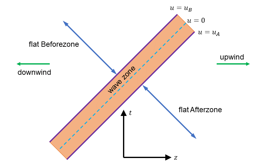
Figure 1: Schema of a sandwich wave (adapted from ref.BoPi89 ) propagating downwind. $u=(z-t)/\sqrt{2}$ is a null coordinate. The space-time is flat in the yet undisturbed Beforezone $u<u_{B}$ and also in the Afterzone $u_{A}<u$ where the wave has already passed.

Our paper studies the geodesic motion of spinless test particles in a sandwich wave GibbHaw71 in a frame where those particles are at rest before the wave reaches them,

$$\dot{{\bf x}}(u)=0\,{\;\;\text{\small for}\;\;}u\leq u_{B}\,.$$ (I.1)

We shall call them special geodesics. (Bondi and Pirani BoPi89 call them “basic geodesics”.)

50 years ago Jean-Marie Souriau has also studied particle motion in a gravitational wave . He presented his pioneering results a year before Zel’dovich et al. at a CNRS meeting held in Paris Sou73 in a paper characteristic for its author: he wrote it in French, used his personal notations and ignored mainstream work. His paper is hidden in an obscure conference proceedings and has never been published in any Journal. It would probably have got totally forgotten had Christian Duval, Souriau’s former student, not remembered and resurrected it many years later Duval17 ; Carroll4GW . The Souriau-Duval approach is summarized in sec.II.

Plane gravitational waves have long been known to admit a generically 5-parameter isometry group Bondi57 ; BoPiRo ; exactsol . In the coordinate system proposed by Baldwin, Jeffery, and by Rosen (BJR) BaJeRo , three of them are mere translations. The remaining two rather mysterious ones have only been known implicitly as solutions of a Sturm-Liouville (SL) equation Torre . The multiple rôles played by Sturm-Liouville is emphasised, e.g., in SLC ; ZCEH ; zzh .

Those two “missing” isometries had been identified in Sou73 using a remarkable tool we refer to as the Souriau matrix, ${\mathfrak{S}}$ in (III.2). His results have long remained confidential and ignored, though.

Another seminal result concerns the group structure related to another recently resurrected topic that young Jean-Marc Lévy-Leblond had called, with tongue in cheek, the “Carroll group” Leblond ; Alice . See Carrollvs ; DH-NC ; Bekaert ; Morand for further developments.

Theorem : The isometries of a plane gravitational wave span the Carroll group without transverse rotations, implemented through the Souriau matrix ${{\mathfrak{S}}}$, see eqns. (III.2)-(III.8).

The geodesics are determined by the conserved quantities associated with the isometries (see sec. IV) , using the Souriau matrix ${{\mathfrak{S}}}$, which is a key ingredient Sou73 ; Carroll4GW .

In sec.V the general theory is illustrated first by a simple Gaussian wave, and then by linearly GibbHaw71 , and finally circularly polarized exactsol ; SLC sandwich waves. For simplicity, we restrict our attention at Beforezones which are flat Minkowski space.

A concept which plays a fundamental role in our investigations is that of a Bargmann manifold , which is a manifold with a metric with Lorentz signature, endowed also with a covariantly constant null vector Eisenhart ; DBKP ; DGH91 ; CDGH , see the Appendix A for a summary.

II Plane gravitational waves

II.1 Baldwin-Jeffery-Rosen (BJR) coordinates

Much of this section is taken from refs. Duval17 ; LongMemory . Following Souriau Sou73 , we write the metric in Baldwin-Jeffery-Rosen (BJR) coordinates $({\bf x},u,v),\,{\bf x}=(x^{1},x^{2})$ BaJeRo ,

$$\mathrm{g}=a_{ij}(u)dx^{i}dx^{j}+2du\,dv\,,$$ (II.1)

where the symmetric positive $2\times 2$ matrix $\mathfrak{a}=\big{(}a_{ij}\big{)}$ depends only on (retarded) time, $u=(z-t)/\sqrt{2}$. Both $u$ and $v=(z+t)/\sqrt{2}$ are null coordinates. The vector $\xi=\partial/\partial v$ is covariantly constant. Thus (II.1) is the metric of a Bargmann manifold Eisenhart ; DBKP ; DGH91 ; ZHAGK ; CDGH . The only nonzero components of its Riemann tensor are

$$R_{uiuj}=-\frac{1}{2}r_{ij}{\quad\text{\small where}\quad}r_{ij}=\Big{(}\ddot{\mathfrak{a}}-\frac{1}{2}\dot{\mathfrak{a}}{\mathfrak{a}}^{-1}\dot{\mathfrak{a}}\Big{)}_{ij}\,$$ (II.2)

($\dot{\mathfrak{a}}=d{\mathfrak{a}}/du$). The metric is thus determined by the symmetric $2\times 2$ matrix $\mathfrak{r}=\big{(}r_{ij}\big{)}$. The only nonzero component of the Ricci tensor is thus,

$$R_{uu}=-\frac{1}{2}\mathrm{Tr}\left(\dot{\mathfrak{b}}+\frac{1}{2}{}{\mathfrak{b}}^{2}\right){\quad\text{\small where}\quad}\mathfrak{b}={\mathfrak{a}}^{-1}\dot{\mathfrak{a}}\,.$$ (II.3)

In the “Before” and “Afterzones”, $u\leq u_{B}$ and $u_{A}\leq u$, respectively, the metric is flat. The most general flat metrics of the form (II.1) is found by setting $\mathfrak{r}=0$ in (II.2) which implies,

$$\dddot{\mathfrak{a}}=0\,,$$ (II.4)

hence $\mathfrak{a}(u)$ is at most quadratic in $u$ and is determined by the initial conditions at some $u_{0}$, $\mathfrak{a}_{0}=\mathfrak{a}(u_{0})$ and $\dot{\mathfrak{a}}(u_{0})=\dot{\mathfrak{a}}_{0}\,,$

$$\mathfrak{a}(u)=\mathfrak{a}_{0}+\dot{\mathfrak{a}}_{0}(u-u_{0})+\frac{1}{4}\dot{\mathfrak{a}}_{0}\mathfrak{a}_{0}^{-1}\dot{\mathfrak{a}}_{0}(u-u_{0})^{2}\,.$$ (II.5)

Denoting a square-root of the matrix $\mathfrak{a}_{0}$ by ${{\mathfrak{P}}}_{0}$, ${{\mathfrak{P}}}_{0}^{\dagger}{{\mathfrak{P}}}_{0}=\mathfrak{a}_{0}$ , we can write Sou73 ,

$$\;\;\displaystyle{\mathfrak{a}(u)={{\mathfrak{P}}}_{0}\Big{(}\mathds{I}+(u-u_{0})\mathfrak{c}_{0}\Big{)}^{2}{{\mathfrak{P}}}_{0}\qquad\text{where}\qquad\mathfrak{c}_{0}=\frac{1}{2}{}{{\mathfrak{P}}}_{0}^{-1}\dot{\mathfrak{a}}_{0}\,{{\mathfrak{P}}}_{0}^{-1}\,.}\;\;$$ (II.6)

In the Beforezone where $\mathfrak{a}_{0}=\mathds{I}=\mathrm{diag}(1,1)$ is the $2\times 2$ unit matrix and $\dot{\mathfrak{a}}_{0}=0$, we duly get $\mathfrak{a}(u)=\mathds{I}$, but in the Afterzone the with non-trivial initial velocity $\mathfrak{c}_{0}\neq 0$ our flat metric (II.6) is clearly more general than mere Minkowski space.

Flat BJR coordinates $({\hat{\mathbf{x}}},{\hat{u}},\hat{v})$ can be introduced outside the Wavezone i.e., for $u\leq u_{B}$ and for $u_{A}\leq u$ Duval17 . In both regions,

$$\begin{array}[]{c}{\bf x}\\ {u}\\ {v}\end{array}\quad\longmapsto\quad\begin{array}[]{l}{\hat{\mathbf{x}}}=\Big{(}\mathds{I}+(u-u_{0})\mathfrak{c}_{0}\Big{)}{{\mathfrak{P}}}_{0}{\bf x}\\ {\hat{u}}=u\\ \hat{v}=v-\frac{1}{2}{\bf x}^{\dagger}{}{{\mathfrak{P}}}_{0}\mathfrak{c}_{0}\Big{(}\mathds{I}+(u-u_{0})\mathfrak{c}_{0}\Big{)}{{\mathfrak{P}}}_{0}{\bf x}\end{array}\,$$ (II.7)

brings the metric (II.1) to the flat form,

$$\mathrm{g}=d{\bf x}^{\dagger}{}\mathfrak{a}(u)d{\bf x}+2du\,dv=d{\hat{\mathbf{x}}}^{\dagger}{}d{\hat{\mathbf{x}}}+2d{\hat{u}}\,d\hat{v}\,.$$ (II.8)

In the Beforezone where $\mathfrak{a}_{0}=\mathds{I}$ and $\mathfrak{c}_{0}=0$, (II.7) is the identity transformation. However in the Afterzone $u\geq u_{A}$ the initial velocity does not vanish in general, $\mathfrak{c}_{0}\neq 0$. Therefore the transition between the flat Before and Afterzones may be non-trivial, – and this is precisely the crux of the story for scattering by a gravitational wave .

Let us now turn to the metric inside the Wavezone $[u_{B},u_{A}]$. By (II.3), Ricci flatness is equivalent to

$$\mathrm{Tr}\left(\dot{\mathfrak{b}}+\frac{1}{2}{}\mathfrak{b}^{2}\right)=0\,.$$ (II.9)

Setting Sou73

$$\chi=\big{(}\det{\mathfrak{a}}\big{)}^{\frac{1}{4}}>0\,{\quad\text{\small and}\quad}\gamma=\chi^{-2}\mathfrak{a}$$ (II.10)

yields $\mathfrak{b}=\gamma^{-1}\dot{\gamma}+2\chi^{-1}\dot{\chi}\,\mathds{I}$ . Then $\det(\gamma)=1$ implies that $\mathrm{Tr}(\gamma^{-1}\dot{\gamma})=0$; thus we end up with a Sturm-Liouville equation Sou73 ; Carroll4GW

$$\;\;\displaystyle{\ddot{\chi}+\omega^{2}(u)\chi=0,\qquad\omega^{2}=\frac{1}{8}\mathrm{Tr}\left((\gamma^{-\frac{1}{2}}\dot{\gamma}\gamma^{-\frac{1}{2}})^{2}\right)\,,}\;\;$$ (II.11)

which guarantees that the vacuum Einstein equations are satisfied for an otherwise arbitrary choice of the unimodular symmetric $2\times 2$ matrix $\gamma(u)$.

Outside the Wavezone, the frequency $\omega$ vanishes (as it will be illustrated in FIG.15), and the Sturm-Liouville equation (II.11) reduces to the free equation,

$$\ddot{\chi}\approx 0\Rightarrow\chi=cu+d\,,$$ (II.12)

which vanishes at most once unless it is identically zero, as it happens in the Before, but not in the Afterzone. Moreover, as argued by Souriau Sou73 , eqn. (II.11) implies that $\chi$ is concave, $\ddot{\chi}<0$, and therefore the determinant of the metric necessarily vanishes at some $u_{1}>u_{B}$

$$\chi(u_{1})=0{\quad\Rightarrow\quad}\det{\mathfrak{a}}(u_{1})=0\,.$$ (II.13)

At $u_{1}$ the BJR expression (II.1) becomes singular, allowing us to conclude that the BJR coordinates are necessarily local i.e. defined only in coordinate patches, defined by the subsequent zeros of $\mathfrak{a}$ — whereas the waves themselves are perfectly well-defined and regular (as it will be seen below using Brinkmann coordinates). The apparent singularity comes from the choice of the coordinates, not from the wave itself. See also Wang:2018iig for a recent discussion.

Had Souriau’s insight been known and appreciated, it could have shortened the controversy .

II.2 Plane gravitational waves in Brinkmann coordinates

An exact plane gravitational wave can also be presented in Brinkmann coordinates Brink $({\bf X},U,V)$,

$$ds^{2}= \;\delta_{ij}dX^{i}dX^{j}+2dUdV+K_{ij}(U)X^{i}X^{j}dU^{2}\,,$$ (II.14a)

$$K_{ij}(U){X^{i}}{X^{j}}= \;\frac{1}{2}{{\mathcal{A}_{+}}}(U)\big{(}(X^{1})^{2}-(X^{2})^{2}\big{)}+{\mathcal{A}_{\times}}(U)\,X^{1}X^{2}\,,$$ (II.14b)

where ${\mathcal{A}_{+}}$ and ${\mathcal{A}_{\times}}$ are the $+$ and $\times$ polarization-state amplitudes. The symmetric and traceless matrix ${\mathds{K}}=(K_{ij})$ is the Brinkmann profile matrix. The only non-vanishing components of the Riemann tensor are, up to symmetry,

$$R_{iUjU}(U)=-K_{ij}(U)$$ (II.15)

(cf. (II.2)). unlike their BJR counterparts, Brinkmann coordinates are global Bondi57 ; BoPiRo .

The “vertical” vector ${\partial}_{V}$ is covariantly constant, — thus we have a Bargmann manifold Eisenhart ; DBKP ; DGH91 , with the quadratic coefficient of the $dU^{2}$ term in (II.14b) interpreted, in the Bargmann framework, as an effective oscillator potential, see the Appendix A.

The relation of the two coordinate systems is established in three steps Gibb75 .

1. Starting with the Brinkmann profile, we first solve (generally only numerically) the Sturm-Liouville equation with a supplementary condition,

   $$\;\;\displaystyle{\ddot{{{\mathfrak{P}}}}={{\mathds{K}}}{{\mathfrak{P}}},\qquad{{\mathfrak{P}}}^{\dagger}\dot{{{\mathfrak{P}}}}=\dot{{{\mathfrak{P}}}^{\dagger}}{{\mathfrak{P}}}\,}\;\;$$ (II.16)

   for some $2\times 2$ matrix ${{\mathfrak{P}}}={\tiny\left(\begin{array}[]{ll}P_{11}&P_{12}\\ P_{21}&P_{22}\end{array}\right)}$; here $\dot{\{\,\}}=d/dU$.

2. Then the symmetric $2\times 2$ matrix

   $$\mathfrak{a}={\small\left(\begin{array}[]{rl}a_{11}&a_{12}\\ a_{21}&a_{22}\end{array}\right)}={{\mathfrak{P}}}^{\dagger}{}{{\mathfrak{P}}}\,={\small\left(\begin{array}[]{ccc}P_{11}^{2}+P_{21}^{2}&&P_{11}P_{12}+P_{21}P_{22}\\[2.0pt] P_{11}P_{12}+P_{21}P_{22}&&P_{22}^{2}+P_{12}^{2}\end{array}\right)}$$ (II.17)

   is the BJR profile.

3. Brinkmann and BJR coordinates, $({\bf X},U,V)$ and $({\bf x},u,v)$, respectively, are related according to,

   $${{\bf X}}={{\mathfrak{P}}}(u){\bf x},\qquad U=u,\qquad V=v-\frac{1}{4}{\bf x}\cdot\dot{\mathfrak{a}}(u){\bf x}\,.$$ (II.18)

   Conversely, the Brinkmann profile ${{\mathds{K}}}=(K_{ij})$ can be recovered from the BJR profile $\mathfrak{a}=(a_{ij})$ by,

   $${{\mathds{K}}}=\frac{1}{2}{}{{\mathfrak{P}}}\left(\dot{\mathfrak{b}}+\frac{1}{2}{\mathfrak{b}}^{2}\right){{\mathfrak{P}}}^{-1}\,,\qquad\mathfrak{b}=\mathfrak{a}^{-1}\dot{\mathfrak{a}}\,,$$ (II.19)

   cf. (II.3).

Now $\det(\mathfrak{a})=\det({{\mathfrak{P}}}^{\dagger})\det({{\mathfrak{P}}})=(\det{{\mathfrak{P}}})^{2}$ implies that BJR coordinates are (unlike their Brinkmann counterparts) defined only on coordinate patches between adjacent zeros $u_{k}$ and $u_{k+1}$ of the determinant of ${{\mathfrak{P}}}$ (or of $\mathfrak{a}$), as said earlier.

Saying that the Beforezone is undisturbed amounts to saying that the BJR profile in (II.1) is $\mathfrak{a}(u)=\mathds{I}$  for $u<u_{B}$, or symbolically,

$$\mathfrak{a}(-\infty)=\mathds{I}\,.$$ (II.20)

II.3 An internal structure ?

Our framework has a curious extra freedom: the “square root matrix” ${{\mathfrak{P}}}$ can be changed by an internal rotation which may depend on $U$ but not on ${\bf x}$. Duval Duval17 has observed that if ${{\mathfrak{P}}}$ is a square root, $\mathfrak{a}={{\mathfrak{P}}}^{\dagger}{{\mathfrak{P}}}$, and $R\in{\rm O}(2)$ is an arbitrary orthogonal matrix, $R^{\dagger}R=RR^{\dagger}=\mathds{I}$, then $(R{{\mathfrak{P}}})^{\dagger}R{{\mathfrak{P}}}={{\mathfrak{P}}}^{\dagger}{{\mathfrak{P}}}=\mathfrak{a}$ and thus

$$\widetilde{{\mathfrak{P}}}=R\,{{\mathfrak{P}}}$$ (II.21)

is another square root, $\widetilde{{\mathfrak{P}}}^{\dagger}\widetilde{{\mathfrak{P}}}=\mathfrak{a}$. Eqns (II.17) and (II.18) imply that the matrix $R$ can be at most a function of $U=u$, $R=R(U)$.

What is the effect of a rotation by $R\in{\rm O}(2)$ ? Firstly, our gauge freedom (II.21) can be use to “dress” ${{\mathfrak{P}}}$ in the Beforezone : a suitable $R$ brings ${{\mathfrak{P}}}(-\infty)$ to the form,

$${{\mathfrak{P}}}(u)=\mathrm{diag}(1,1){\;\;\text{\small for}\;\;}u\leq u_{B}\,,\quad\text{\small symbolically }\quad{{\mathfrak{P}}}(-\infty)=\mathrm{diag}(1,1)\,,$$ (II.22)

Secondly, the redefinition (II.21) affects the BJR $\leftrightarrow$ B correspondence, which is in fact multivalued : a BJR metric can be mapped into many different Brinkmann metrics by changing $R$.

$\bullet$ When $R$ is a constant matrix then (II.18) becomes,

$$X^{i}=(R^{\dagger}\widetilde{{\mathfrak{P}}})^{i}_{\,j}x^{j},\quad U=u,\quad V=v-\frac{1}{4}x^{i}x^{j}\dot{a}_{ij}\,.$$ (II.23)

Note that the last term here does not change because $\widetilde{{\mathfrak{P}}}$ is a square root of $\mathfrak{a}$.

The SL problem (II.16) becomes in turn,

$$\ddot{\widetilde{{\mathfrak{P}}}}_{ij}=\big{(}R{{\mathds{K}}}R^{\dagger}\big{)}_{ik}\widetilde{{\mathfrak{P}}}^{k}_{\,j}\,,\qquad(\widetilde{{\mathfrak{P}}})^{\dagger}\dot{\widetilde{{\mathfrak{P}}}}=(\dot{\widetilde{{\mathfrak{P}}}})^{\dagger}\,\widetilde{{\mathfrak{P}}}\,.$$ (II.24)

Then, in terms of the new (transverse) coordinate

$$\widetilde{X}^{i}=R^{i}{}_{j}X^{j}\,,$$ (II.25)

the Brinkmann metric (II.14a) is written as,

$$ds^{2}=\delta_{ij}d\widetilde{X}^{i}d\widetilde{X}^{j}+2dUdV+\widetilde{K}_{ij}\widetilde{X}^{i}\widetilde{X}^{j}dU^{2}\,,\qquad\widetilde{K}_{ij}=\big{(}RKR^{\dagger}\big{)}_{ij}\,.$$ (II.26)

$\bullet$ When the ${\rm O}(2)$ matrix $R$ is $U\equiv u$-dependent, $\dot{R}\neq 0$, the situation gets more subtle. The B $\Leftrightarrow$ BJR coordinate transformation generates a gauge potential, (see Appendix A).

We illustrate this point on a circularly polarized periodic (CPP) PolPer gravitational wave, whose Sturm-Liouville equation (II.16) was solved in Zhang:2018msv ; Elbistan:2022umq . The Brinkmann metric (II.14) is (II.14a) with profile,

$$K_{ij}(U)X^{i}X^{j}=\frac{A_{0}}{2}\Big{(}\cos(\omega U)\big{(}(X^{1})^{2}-(X^{2})^{2}\big{)}+2\sin(\omega U)X^{1}X^{2}\Big{)}\,,$$ (II.27)

where $A_{0}$ is the amplitude and $\omega$ is the frequency of the wave. Then, by following a suggestion of Kosinski Kosinski and further developed in refs.PolPer ; ZHAGK ; AndrPrenc , we switch to rotating coordinates $\widetilde{{\bf X}}$ (II.25) but now with a $U$-dependent transverse rotation i.e., $\widetilde{X}^{i}=R^{i}{}_{j}(U)X^{j}$ ,

$$\begin{pmatrix}\tilde{X}^{1}\\ \tilde{X}^{2}\end{pmatrix}=\begin{pmatrix}\cos({\frac{1}{2}}\omega U)&\sin({\frac{1}{2}}\omega)\\[4.0pt] -\sin({\frac{1}{2}}\omega U)&\cos({\frac{1}{2}}\omega U)\,\end{pmatrix}\begin{pmatrix}X^{1}\\ X^{2}\end{pmatrix}\,,$$ (II.28)

where $U$ and $V$ are kept fixed. The $U$-dependent rotation (II.28) belongs to $\mathrm{SO}(2)$ which does not change neither the associated BJR metric $\mathfrak{a}$ and consequently nor the geodesic motion.

When $R=R(U)$, then $d\tilde{X}^{i}=R^{i}{}_{j}dX^{j}+\dot{R}^{i}{}_{j}X^{j}dU$ and the metric picks up additional terms. For our CPP wave we find,

$$ds^{2}= \;\delta_{ij}d\widetilde{X}^{i}d\widetilde{X}^{j}+2dUdV+\omega\epsilon_{ij}\widetilde{X}^{i}d\widetilde{X}^{j}dU+\Big{(}\Omega_{+}^{2}(\widetilde{X}^{1})^{2}+\Omega_{-}^{2}(\widetilde{X}^{2})^{2}\Big{)}dU^{2},$$ (II.29a)

$$\Omega_{\pm}^{2}= \;\frac{\omega^{2}}{4}\pm\frac{A_{0}}{2}\,.$$ (II.29b)

From the Bargmann point of view Eisenhart ; DBKP ; DGH91 ; ZHAGK , (see the Appendix A for a summary) this metric describes an anisotropic oscillator with shifted but $U$-independent frequencies , augmented by a new, linear-in-$\widetilde{{\bf X}}$ gauge potential term,

$$2{\bf A}{\cdot}d\widetilde{{\bf X}}=\omega\epsilon_{ij}\widetilde{X}^{i}\;d\widetilde{X}^{j}dU\,,$$ (II.30)

[where $\epsilon_{ij}$ is the antisymmetric Levi-Civita symbol], whose curvature is

$${\mathcal{F}}=d{\bf A}=\omega\,d\widetilde{X}^{1}\wedge d\widetilde{X}^{2}\,.$$ (II.31)

Thus for $\omega\neq 0$ ${\bf A}$ is not a pure gauge and does therefore have an effect on the geodesic dynamics : — it is indeed the source of the Coriolis force ZHAGK . The potential can be either attractive or repulsive, depending on the relative strength of the two terms in (II.29b). The middle, Coriolis term is always attractive, though, and if it is strong enough, it can bound all motions, as in FIGs.2 and 3.

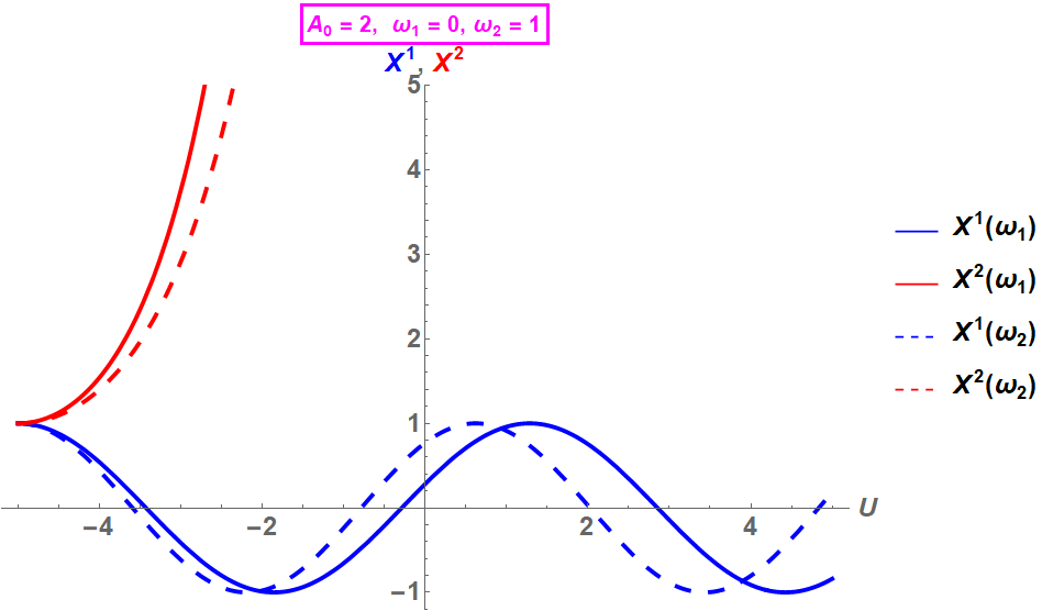
Figure 2: Trajectories for $A_{0}=2$, and for either $\omega_{1}=0$ or for $\omega_{2}=1$ . When ${\bm{\omega}}_{1}=0$, one of the oscillators in the last term is attractive and the is other repulsive; the tractories (shown in full lines) are, accordingly, bounded or unbounded. The trajectory (shown in dotted line) is different is however qualitatively similar for ${\bm{\omega}}_{2}=1$,

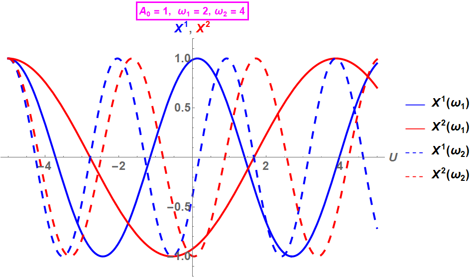
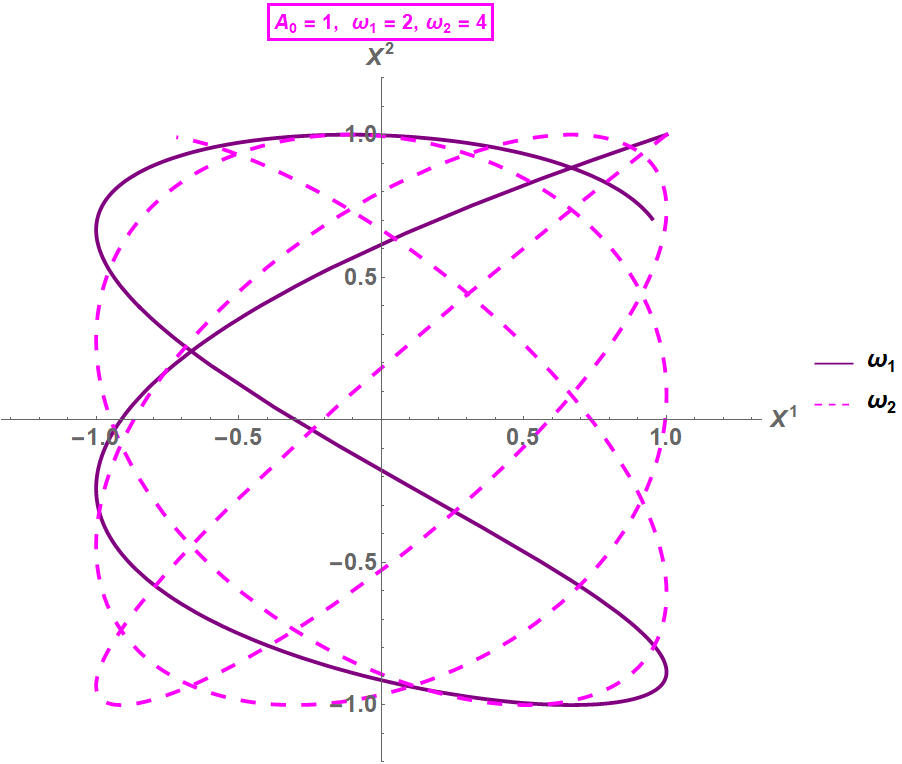
Figure 3: Trajectories for $A_{0}=1,\,\omega_{1}=2,\,\omega_{2}=4$ . For (relatively) large $\omega$ and small $A_{0}$, both frequencies $\Omega_{\pm}>0$ but are dominated by the strong Coriolis force: motions are bounded.

The new term (II.30) changes also the Sturm-Liouville equation (II.16) which swaps the Brinkmann and BJR metrics,

$$\ddot{\widetilde{{\mathfrak{P}}}}=\Omega\,\widetilde{{\mathfrak{P}}}+\omega\epsilon\,\dot{\widetilde{{\mathfrak{P}}}}\,,\qquad\Big{(}\widetilde{{\mathfrak{P}}}^{\dagger}\dot{\widetilde{{\mathfrak{P}}}}-\dot{\widetilde{{\mathfrak{P}}}}^{\dagger}\widetilde{{\mathfrak{P}}}\Big{)}=\omega\widetilde{{\mathfrak{P}}}^{\dagger}\epsilon\widetilde{{\mathfrak{P}}}\,,$$ (II.32)

where $\epsilon$ is the anti-symmetric Levi-Civita matrix and

$$\Omega=\begin{pmatrix}\Omega_{+}^{2}&0\\ 0&\Omega_{-}^{2}\end{pmatrix}\,$$ (II.33)

with $\Omega_{\pm}$ given in (II.29b).

Example: Lukash metric: At this point, it is instructive to recall what happens for the Lukash metric Lukash ; LukashI . Switching provisionally to the notations of ref. LukashII , for $U>0$ the metric (to be compared with the CPP case (II.27)) is,

$$ds^{2}_{L} = d{\bf X}^{2}+2dUdV$$ (II.34)

$$- \left\{\frac{C}{U^{2}}\cos\Big{(}2\kappa\ln(U)\Big{)}\,\big{[}(X^{1})^{2}-(X^{2}]^{2}\big{)}\,-\,\frac{2C}{U^{2}}\sin\Big{(}2\kappa\ln(U)\Big{)}\,X^{1}X^{2}\right\}\,dU^{2}\,.\qquad\quad$$

Then the coordinate transformation zzh

$$U=e^{T}\,,\quad\bm{X}=e^{T/2}\bm{\xi},\quad V\to V,{\quad\text{\small where}\quad}\bm{\xi}=(\xi,\eta)$$ (II.35)

yields which is conformal, $ds_{L}^{2}=e^{\dagger}d\Sigma^{2}\,,$ to

$$d\Sigma^{2} = d\xi^{2}+d\eta^{2}+2dTdV+\big{(}{\xi}d\xi+{\eta}d\eta\big{)}dT+$$ (II.36)

$$\left(\frac{1}{4}\left(\xi^{2}+\eta^{2}\right)-C\left(\xi^{2}-\eta^{2}\right)\cos 2\kappa T+2C\xi\eta\sin 2\kappa T\right)dT^{2}\,.$$

(Remember that conformal metrics have identical null geodesics and are also simply related massive ones ZCEH ; nonlocal ). Our clue is that the $d\xi^{i}dT$ term is a pure gauge,

$${\bf A}=A_{i}d\xi^{i}=\xi^{i}d\xi^{i}=\frac{1}{2}d\big{(}\xi^{i}\xi^{i}\big{)}{\quad\Rightarrow\quad}{\mathcal{F}}=d{\bf A}=0\,.$$ (II.37)

The associated magnetic field vanishes, and therefore the vector potential ${\mathcal{A}}$ has no effect on the geodesic motion. It can in fact be gauged away by a redefinition of the coordinate $V$, $V\to v-\frac{1}{4}\xi^{i}\xi^{i}$ LukashII .

The difference between the two cases is also understood by observing that, unlike as for CPP, for Lukash the component oscillators in (II.29b) have no relative minus sign and therefore can be gauged away by a redefinition of the $V$-coordinate.

We note for completeness that rotation with an $U$-dependent matrix $R(U)\in{\rm O}(2)$ would yield a modified Sturm-Liouville equation of rather complicated form,

$$\ddot{\widetilde{{\mathfrak{P}}}}=(R{\mathds{K}}R^{\dagger})\widetilde{{\mathfrak{P}}}+\dot{R}(\dot{R^{\dagger}}\widetilde{{\mathfrak{P}}}+2R^{\dagger}\dot{\widetilde{{\mathfrak{P}}}}),\qquad\widetilde{{\mathfrak{P}}}^{\dagger}\dot{\widetilde{{\mathfrak{P}}}}-\dot{\widetilde{{\mathfrak{P}}}}^{\dagger}\widetilde{{\mathfrak{P}}}=2\widetilde{{\mathfrak{P}}}^{\dagger}\dot{R}R^{\dagger}\widetilde{{\mathfrak{P}}}\,,$$ (II.38)

cf. (II.32). In conclusion, the $U$-dependent rotation (II.21) alters the Brinkmann metric (IV.29) and consequently the geodesic motion, while keeping the BJR metric unchanged, $\mathfrak{a}=\widetilde{{\mathfrak{P}}}^{\dagger}\widetilde{{\mathfrak{P}}}={\mathfrak{P}}^{\dagger}{\mathfrak{P}}$. In other words, the B $\leftrightarrow$ BJR correspondence is many-to-one.

III Carroll symmetry of plane gravitational waves

It has long been known that the metric (II.1) has a (generically $5$-parameter) isometry group, composed of manifest ${\bf x}$ and $v$-translations, ${\bf x}\to{\bf x}+{\mathbf{c}}$ and $v\to v+d$, respectively, augmented by a rather mysterious 2-parameter subgroup BoPiRo ; exactsol . Apparently ignoring the existing results, the latter has been identified by Souriau in his “well hidden” conference paper Sou73 – but the rôle and its relation to Carroll symmetry Leblond were established only recently Duval17 ; Carrollvs ; Carroll4GW ; ZHAGK . The isometry group BoPiRo is generated by the Killing vectors, written, in BJR coordinates,

$$Y^{v}=\frac{\partial}{\partial v}\,,\qquad Y^{i}_{c}=\delta^{ij}\frac{\partial}{\partial x^{j}}\,,\qquad Y^{i}_{b}=S^{ij}(u)\frac{\partial}{\partial x^{j}}-x^{i}\frac{\partial}{\partial v}\,.$$ (III.1)

Anticipating our results to come, the $Y^{i}_{b},\,i=1,2$ will be referred to as Carroll boosts. A crucially important role is played here by the symmetric $2\times 2$ Souriau matrix

$${{\mathfrak{S}}}(u)\equiv(S_{ij})=\displaystyle{\int^{u}_{u_{0}}}\!\!\mathfrak{a}^{-1}(t)dt\,,\qquad u_{k}<u_{0},\,u<u_{k+1}\,,$$ (III.2)

which depends only on $\mathfrak{a}={{\mathfrak{P}}}^{\dagger}{{\mathfrak{P}}}>0$. Therefore we get, for all choices of the orthogonal matrix $R$, the same Souriau matrix: the “gauge freedom” ${\mathfrak{P}}\to R\,{\mathfrak{P}}$ in (II.21) disappears — just as it happens when passing from a gauge potential to the field strength tensor.

Each component of the Souriau matrix satisfies the same Sturm-Liouville equation with the appropriate auxiliary condition (II.16) as ${\mathfrak{P}}$ does SLC ; ZCEH . Keeping this in mind, let us pull back the Carroll Killing vectors (III.1) to Brinkmann coordinates $X^{\mu}=\{X^{i},U,V\}$ using (II.18). The vector fields (III.1) become,

$$Y=Y^{\nu}(X(x))\frac{\partial X^{\mu}}{\partial x^{\nu}}\frac{\partial}{\partial X^{\mu}}\,.$$ (III.3)

$\bullet$ For $v$-translation (III.1) we get the covariantly constant null Killing vector written in Brinkmann coordinates,

$$Y^{v}=\frac{\partial}{\partial v}=\frac{\partial U}{\partial v}\frac{\partial}{\partial U}+\frac{\partial X^{i}}{\partial v}\frac{\partial}{\partial X^{i}}+\frac{\partial V}{\partial v}\frac{\partial}{\partial V}=\frac{\partial}{\partial V}\,.$$ (III.4)

$\bullet$ $x$-translations (III.1) become ,

$$Y^{i}_{c}=\frac{\partial}{\partial x^{i}}={\mathfrak{P}}^{ji}\frac{\partial}{\partial X^{j}}-\frac{1}{2}\dot{\mathfrak{a}}_{ij}x^{j}\frac{\partial}{\partial V}={\mathfrak{P}}^{ji}\frac{\partial}{\partial X^{j}}-\dot{{\mathfrak{P}}}_{j}{}^{i}X^{j}\frac{\partial}{\partial V}\,,$$ (III.5)

where the subsidiary condition (II.16) was used. Thus the ${\mathfrak{P}}$-matrix (II.16) generates Carroll translations in Brinkmann coordinates.

$\bullet$ At last, Carroll boosts $Y^{i}_{b}$ (III.1) are expressed, in Brinkmann coordinates, as,

$$Y^{i}_{b}=({\mathfrak{P}}{\mathfrak{S}})^{ji}\frac{\partial}{\partial X^{j}}-\dot{({\mathfrak{P}}{\mathfrak{S}})}_{j}{}^{i}X^{j}\frac{\partial}{\partial V}\,,$$ (III.6)

where the matrix ${\mathfrak{P}}{\mathfrak{S}}$ that shares the same properties with the matrix ${\mathfrak{P}}$, generates Carroll boosts. In concusion, Torre’s expression Torre is recovered. (III.5) and (III.6) can be unified into a a compact form,

$$Y^{i}=Q^{ji}\frac{\partial}{\partial X^{j}}-\dot{Q}_{j}{}^{i}X^{j}\frac{\partial}{\partial V}\,,$$ (III.7)

where $Q_{ij}=P_{ij}$ for translations and $Q_{ij}=({{\mathfrak{P}}}{{\mathfrak{S}}})_{ij}$ for boosts. Conversely, the $\dot{Q}_{j}{}^{i}$ factor here gets absorbed under the inverse transformation $V\to v$, (III.1) LukashI , as recalled above.

Eqn. (III.7) is just (III.1) translated to Brinkmann coordinates, however while (III.1) is simple and valid for any BJR profile, (III.7) requires to solve the Sturm-Liouville equation for ${\widetilde{\mathfrak{P}}}=(Q_{ij})$. This underlines the advantage of using BJR coordinates to determine the symmetries of plane waves.

Henceforce we restrict our investigations to an interval $I_{k}=[u_{k},u_{k+1}]$ chosen between two adjacent zeros of $\det(\mathfrak{a})$ [equivalently, of $\det({{\mathfrak{P}}})$] and we pick a point $u_{0}\equiv u_{0}^{(k)}\in I_{k}$. The three translation are trivial, therefore we focus our attention at the 2-parameter subgroup generated by the C-boosts, $Y^{i}_{b}$ in (III.1). In BJR terms, the latter acts on space-time at fixed $u$, according to

$${\bf x}\to{\bf x}+{{\mathfrak{S}}}(u){\mathbf{b}}\,,\qquad u\to u,\qquad v\to v-{\mathbf{b}}\cdot{\bf x}-{\hbox{$\textstyle\frac{1}{2}$}}{\mathbf{b}}\cdot{}{{\mathfrak{S}}}(u){\mathbf{b}}\,.$$ (III.8)

In Minkowski space, for example, $\mathfrak{a}$ is the unit matrix $\mathds{I}$. Now $\dot{{\mathfrak{S}}}={\mathfrak{a}}^{-1}=\mathds{I}$, hence

$${{\mathfrak{S}}}(u)=(u-u_{0})\mathds{I}\,,$$ (III.9)

so that (III.8) reduces to Galilei boosts in $2+1$ dimensions, lifted to Minkowski space written in light-cone coordinates, viewed as a particular Bargmann manifold with trivial profile $(K_{ij})\equiv 0$ DBKP ; DGH91 .

At the points $u_{k}$ where $\big{(}\det(\mathfrak{a})\big{)}(u_{k})=0$ the matrix $\mathfrak{a}$ is not invertible and ${{\mathfrak{S}}}$ is undefined. Boosts in Brinkmann coordinates are obtained by using (II.18), which, when the profile $(K_{ij})$ is non-trivial, have a distorted implementation, as it will be illustrated in FIG.17 in sect.V.

$${\bf X}\to{\bf X}+{{\widetilde{\mathfrak{P}}}}\,{\mathbf{b}}\,,$$ (III.10a)

$$V\to V-{\bf X}\cdot\dot{{\widetilde{\mathfrak{P}}}}\,{\mathbf{b}}-\frac{1}{2}{\widetilde{\mathfrak{P}}}\,{\mathbf{b}}\cdot\dot{{\widetilde{\mathfrak{P}}}}\,{\mathbf{b}}\,,$$ (III.10b)

where

$${\widetilde{\mathfrak{P}}}(u)={{\mathfrak{P}}}(u){{\mathfrak{S}}}(u)\,.$$ (III.11)

The matrix ${{\widetilde{\mathfrak{P}}}}$ is $u$-dependent, however boosts leave each “vertical” slice $U=u=\mathop{\rm const.}\nolimits$ invariant, as depicted conceptually in FIG.4. Examples will be presented in sec.V.

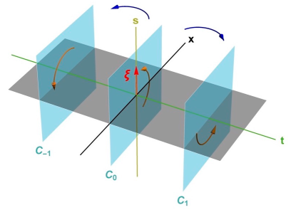
Figure 4: The distorted boosts (III.10) leave the $u=\mathop{\rm const.}\nolimits$ slices invariant, upon which they are implemented through the matrix ${{\widetilde{\mathfrak{P}}}}(u)={{\mathfrak{P}}}(u){{\mathfrak{S}}}(u)$ .

The matrix ${{\widetilde{\mathfrak{P}}}}$ here satisfies the same SL plus auxiliary equation (II.16) as ${{\mathfrak{P}}}$ does SLC ,

$$\ddot{{\widetilde{\mathfrak{P}}}}={{\mathds{K}}}\,{{\widetilde{\mathfrak{P}}}}\,,\qquad{{\widetilde{\mathfrak{P}}}}^{\dagger}\dot{{\widetilde{\mathfrak{P}}}}-\dot{{{\widetilde{\mathfrak{P}}}}^{\dagger}}{{\widetilde{\mathfrak{P}}}}=0\,$$ (III.12)

and then we could repeat our analysis for ${{\mathfrak{P}}}$. It is however more convenient to combine our previous results obtained for ${{\mathfrak{P}}}$ and ${{\mathfrak{S}}}$. In the Beforezone we have (III.9) and the usual lifted Galilean action is recovered. The behavior in the Afterzone is more subtle, as it will be seen in sec.V. The boosted BJR profile is related to the initial $\mathfrak{a}$ by a similarity transformation,

$$\mathfrak{a}=(a_{ij})\to({\mathfrak{P}}{\mathfrak{S}})^{\dagger}_{\;ik}({\mathfrak{P}}{\mathfrak{S}})^{k}_{\;j}=({\mathfrak{S}}^{\dagger}\mathfrak{a}\,{\mathfrak{S}})_{ij}\,,$$ (III.13)

(${\mathfrak{S}}{\dagger}={\mathfrak{S}}$).

For the flat Minkowski metric, for example, the boosted BJR metric (III.10) with (III.11) reduces to the Souriau matrix, ${\mathfrak{S}}=u\mathds{I}$, which plainly solves the free SL equation $\ddot{{\mathfrak{P}}}=0$. Accordingly in Brinkmann coordinates, ${\widetilde{\mathfrak{P}}}={\mathfrak{P}}{\mathfrak{S}}=u\mathds{I}$ yields the BJR metric

$$g_{\mu\nu}dx^{\mu}dx^{\nu}=u^{2}\delta_{ij}dx^{i}dx^{j}+2dudv\,,$$ (III.14)

whose conform-flatness follows from (II.2) and (II.3), which imply that the Ricci tensor vanishes. This metric is degenerate at $u=0$ ; the Souriau matrix is $\sim u^{-1}$. Choosing $u_{0}\neq 0$ would not change the description.

IV Memory Effect for Geodesics

In globally defined transverse Brinkmann coordinates the geodesics are solutions of

$$\dfrac{d^{2}{\bf X}}{dU^{2}}-\frac{1}{2}\left(\begin{array}[]{lr}{\mathcal{A}}_{+}&{\mathcal{A}}_{\times}\\ {{\mathcal{A}}_{\times}}&-{\mathcal{A}}_{+}\end{array}\right)\,{\bf X}=0\,,$$ (IV.1)

while $V$ satisfies a complicated equation, # (II.3b) in PolPer , we reproduce for completeness,

$$\dfrac{d^{2}V}{dU^{2}} +\dfrac{1}{4}\displaystyle{\frac{d{\mathcal{A}}_{+}}{dU\,}}\big{(}(X^{1})^{2}-(X^{2})^{2}\big{)}+{\mathcal{A}}_{+}\big{(}X^{1}\dfrac{dX^{1}}{dU\,}-X^{2}\dfrac{dX^{2}}{dU\,}\big{)}$$ (IV.2)

$$+\dfrac{1}{2}\dfrac{d{\mathcal{A}}_{\times}}{dU\,}X^{1}X^{2}+{\mathcal{A}}_{\times}\big{(}X^{2}\dfrac{dX^{1}}{dU\,}+X^{1}\dfrac{dX^{2}}{dU\,}\big{)}\,=\,0\,\qquad$$

which is indeed a consequence of the transverse ones.

Eqn (IV.1) is in general a pair of coupled Sturm-Liouville equations that can be solved only numerically. For a linearly polarized wave ${\mathcal{A}}_{\times}=0$ and we denoting simply ${\mathcal{A}}_{+}={\mathcal{A}}$, (IV.1) reduces to two uncoupled SL equations,

$$\dfrac{d^{2}\!{\bf X}}{dU^{2}}-\frac{1}{2}\mathrm{diag}({\mathcal{A}},-{\mathcal{A}})\,{\bf X}=0\,.$$ (IV.3)

In the Bargmann picture Eisenhart ; DBKP ; DGH91 (see Appendix A), the effective linear force ${\mathcal{A}}{\bf X}$ is attractive or repulsive depending on its sign.

Velocity effect: Returning to (IV.1), the total increment of the velocity along the transverse trajectory ${\bf X}(U)=\big{(}X^{1}(U),X^{2}(U)\big{)}$ between the Before and Afterzones is given by eqn. # (3.4) of PolPer ,

$$\Delta\dot{{\bf X}}=\int_{U_{B}}^{U_{A}}\!\!{{\mathds{K}}}(U)\,{\bf X}(U)dU\,=\frac{1}{2}\left(\begin{array}[]{l}\displaystyle\int_{U_{B}}^{U_{A}}\!\!{\small\big{(}{{\mathcal{A}}_{+}}(U)X^{1}(U)+{\mathcal{A}}_{\times}(U)X^{2}(U)\big{)}\,dU}\\[14.0pt] \displaystyle\int_{U_{B}}^{U_{A}}\!\!{\small\big{(}{{\mathcal{A}}_{\times}}(U)X^{1}(U)-{{\mathcal{A}}_{+}}(U)X^{2}(U)\big{)}\,dU}\end{array}\right)\,$$ (IV.4)

which, for a linearly polarized special geodesic (IV.4) reduces to

$$\Delta\dot{{\bf X}}={\small\frac{1}{2}\left(\begin{array}[]{r}\quad\;\displaystyle\int_{U_{B}}^{U_{A}}\!\!{{\mathcal{A}}}_{+}(U)P_{11}(U)X_{0}^{1}\,dU\\[16.0pt] -\!\displaystyle\int_{U_{B}}^{U_{A}}\!\!{{\mathcal{A}}}_{+}(U)P_{22}(U)X_{0}^{2}\,dU\end{array}\right)\,}={\small\frac{1}{2}\left(\begin{array}[]{r}\quad\;\displaystyle\int_{U_{B}}^{U_{A}}\!\!{{\mathcal{A}}}_{+}(U)X^{1}(U)\,dU\\[16.0pt] -\!\displaystyle\int_{U_{B}}^{U_{A}}\!\!{{\mathcal{A}}}_{+}(U)X^{2}(U)\,dU\end{array}\right)\,}.$$ (IV.5)

The variation of the relative (euclidean) distance ${\Delta}_{X}({\bf X},{\bf Y})=|{\bf X}-{\bf Y}|=\sqrt{(X^{1})^{2}+(X^{2})^{2}}$ and of the relative velocity ${\Delta}_{\dot{X}}=|\dot{\bf X}-\dot{\bf Y}|$, shown in FIG.7 confirm the velocity effect: a particle initially at rest is not simply displaced but has a constant nonvanishing residual relative velocity after the wave has passed. This could in principle be observed through the Doppler effect BraGri and is consistent with the Newtonian behavior in transverse space which follows from the Bargmann framework. Illustrations, (confirmed analytically Chakraborty ), will be presented in secs.V, VI and VII.

Further insight is gained by switching to BJR coordinates. First we note that the quantity called the Jacobi invariant,

$$e=\frac{1}{2}\mathrm{g}_{\mu\nu}\,\dot{x}^{\mu}\dot{x}^{\nu}$$ (IV.6)

is conserved for geodesic motion; it is negative/zero/positive for a timelike/null/spacelike geodesic. Here we deal with timelike geodesics and require therefore $e<0$.

The conserved quantities associated with the isometries of the metric are determined by Noether’s theorem. Choosing $u$ as parameter the invariant $e$ in (IV.6) is $e=\frac{1}{2}a_{ij}(u)\dot{x}^{i}\dot{x}^{j}-\dot{v}\,$ and the Noether quantities are, within the domain of the BJR coordinates BoPi89 ,

$${\bm{p}}= \;\mathfrak{a}\,\dot{{\bf x}}\,\qquad \sim{\bf x}$$ momentum -translation (IV.7a)

$$m= \;1\qquad \sim v$$ mass -translation (IV.7b)

$$\mathbf{k}= \;{\bf x}-{{\mathfrak{S}}}{\bm{p}}\,\qquad$$ boost momentum (IV.7c)

Conversely, the conserved quantities determine the geodesics,

$${\bf x}(u)= \quad{{\mathfrak{S}}}(u)\,{\bm{p}}\;+\;\mathbf{k}\,,$$ (IV.8a)

$$v(u)= \;-\frac{1}{2}{\bm{p}}\cdot{{\mathfrak{S}}}(u)\,{\bm{p}}+e\,u+v_{0}\,,$$ (IV.8b)

where $v_{0}$ is yet another integration constant. Thus the only quantity to calculate is the Souriau matrix, ${{\mathfrak{S}}}(u)$ in (III.2). The formulae (IV.8) make sense where ${{\mathfrak{S}}}$ is well-defined i.e., between two adjacent zeros $u_{k}$ and $u_{k+1}$ of $\mathfrak{a}$. We note for later reference that the $v$-equation (IV.8b) is in fact determined by the null lift of (IV.8a) and by the Jacobi invariant $e$ in (IV.6). For massless geodesics $e=0$ (IV.6) the coordinate $v$ is indeed the classical action for the underlying NR system Carroll4GW .

Special geodesics are in rest in the Beforezone, ${\bf x}(u)={\bf x}_{0},u\leq u_{B}\,$. Therefore ${\bm{p}}=0$ by (IV.7a) — and momentum conservation then implies that

$${\bm{p}}=0$$ (IV.9)

for all $u$ in the domain of definition of the coordinates. Thus by (IV.8) we have,

$${\bf x}={\bf x}_{0}=\mathbf{k}\,\qquad\&\qquad v=e\,u+v_{0}\,,$$ (IV.10)

i.e., simple “vertical” motion with fixed transverse position — and that for an arbitrary BJR profile $\mathfrak{a}$ ! We stress that this extreme simplicity is due to our using BJR coordinates.

Returning to Brinkmann coordinates, our special geodesics are instead ,

$${\bf X}(U)= \;{{\mathfrak{P}}}(u){\bf X}_{0}\,,$$ (IV.11a)

$$V(U)= \;v-\frac{1}{2}{\bf X}_{0}({{\mathfrak{P}}}^{\dagger}\dot{{{\mathfrak{P}}}}){\bf X}_{0}+eU+V_{0}\,,$$ (IV.11b)

$V_{0}=\mathop{\rm const.}\nolimits$ Unlike their BJR ancestors, these trajectories can be very complicated due to the complicated forms of the ${{\mathfrak{P}}}$ and ${{\mathfrak{S}}}$ matrices, as will be seen in sec.V (see FIG. 25 for example).

A particular set of special geodesics in Brinkmann coordinates is obtained by choosing the initial position ${\bf x}^{(1)}_{0}={\tiny\left(\begin{array}[]{c}1\\ 0\end{array}\right)}$ and ${\bf x}^{(2)}_{0}={\tiny\left(\begin{array}[]{c}0\\ 1\end{array}\right)}$ in the Beforezone, for which we get the columns of the ${{\mathfrak{P}}}$-matrix,

$${\bf X}^{(1)}(u)={{\mathfrak{P}}}(u){\tiny\left(\begin{array}[]{c}1\\ 0\end{array}\right)}={\tiny\left(\begin{array}[]{c}P_{11}(u)\\[5.0pt] P_{21}(u)\end{array}\right)}{\quad\text{\small and}\quad}{\bf X}^{(2)}(u)={{\mathfrak{P}}}(u){\tiny\left(\begin{array}[]{c}0\\ 1\end{array}\right)}={\tiny\left(\begin{array}[]{c}P_{12}(u)\\[5.0pt] P_{22}(u)\end{array}\right)}\,.$$ (IV.12)

Special geodesics are at rest in the Beforezone, ${{\mathfrak{P}}}=\mathds{I}$, ${\bf X}(U)={\bf X}_{0}\equiv{\bf x}^{0}$ for $U\leq U_{B}$; Our plots in sec.V then confirm that they will be focused, as argued by Bondi and Pirani BoPi89 .

Let ${\bf X}_{a}(U)$ and ${\bf X}_{b}(U)$ be indeed two special geodesics; we show that for appropriate initial conditions there exists an $U_{1}$ such that the two geodesics meet, ${\bf X}_{a}(U_{1})={\bf X}_{b}(U_{1})$ for some finite and universal $U_{1}>U_{B}$. Setting ${\bf X}_{a,b}(U)={\bf X}_{a}(U)-{\bf X}_{b}(U)$ we have ${\bf X}_{a,b}(U)={{\mathfrak{P}}}(u){\bf x}_{a,b}^{0}$, so we need ${\bf x}^{0}={\bf x}_{a}^{0}-{\bf x}_{b}^{0}\neq 0$ in the kernel of ${{\mathfrak{P}}}(u_{1})$,

$${{\mathfrak{P}}}(u_{1}){\bf x}^{0}=0\,.$$ (IV.13)

Then all such geodesics meet at the same $U_{1}\equiv u_{1}$. This requires ${{\mathfrak{P}}}(u_{1})$ to be a singular matrix with a nontrivial kernel, detected by the vanishing of its determinant,

$$\det\big{(}{{\mathfrak{P}}}(u_{1})\big{)}=0\,.$$ (IV.14)

But $\det(\mathfrak{a})=(\det{{\mathfrak{P}}})^{2}=\chi^{4}$ and therefore $\det{{\mathfrak{P}}}=0$ iff $\chi=0$; then Souriau’s proof shows that $\chi$ necessarily vanishes at some $u_{1}\geq u_{B}$.

More generally, consider, for any ${\bf x}_{0}$ ${\bf x}_{0}^{*}={\bf x}_{0}+{\bf x}^{\perp},$ where ${{\mathfrak{P}}}(u_{1}){\bf x}^{\perp}=0\,.$ Then for the geodesic issued from ${\bf x}_{0}^{*}$ we have,

$${\bf X}(u_{1})={{\mathfrak{P}}}(u_{1}){\bf x}_{0}^{*}={{\mathfrak{P}}}(u_{1}){\bf x}_{0}\,,$$ (IV.15)

i.e., all special geodesics whose initial positions differ by a vector ${\bf x}^{\perp}$ end at the same point ${\bf X}(u_{1})={{\mathfrak{P}}}(u_{1}){\bf x}_{0}$ BoPi89 .

The ${{\mathfrak{P}}}$-matrix of a linearly polarized wave is, for example, diagonal, ${{\mathfrak{P}}}=\mathrm{diag}(P_{11},P_{22})$ and the $X^{1}(U)$ (resp. $X^{2}(U)$) components meet at those critical points where $P_{11}(u_{1})=0$ (resp. $P_{22}(u_{2})=0$), as it will be seen in FIG.11 in sec.V.

In conclusion, we have two different ways to find the geodesics: either by using global Brinkmann coordinates which yield regular but complicated trajectories found by solving (numerically) the Sturm-Liouville equations (IV.3).

Alternatively, we can find first our simple geodesics in BJR with help of the Carroll symmetry (IV.8) and then carry them to Brinkmann by (II.18) by using the ${{\mathfrak{P}}}$ matrix. However BJR coordinates are defined only on coordinate patches between adjacent zeros $u_{k}$ and $u_{k+1}$ of the determinant of ${{\mathfrak{P}}}$ (or of $\mathfrak{a}$). Our plots in sect.V show, moreover, that those BJR solutions diverge at the contact points $u_{k}$ and then we have to glue together the bits of trajectories obtained by pulling back to Brinkmann coordinates from the adjacent intervals $I_{k}=[u_{k},u_{k+1}]$ — yielding, remarkably, smooth curves. FIG.18 confirms that we end up with the same result.

IV.1 Hamiltonian and Lagrangian aspects

We complete our investigations with an outline of the Lagrangian and Hamiltonian aspects. The geodesic Lagrangian resp. Hamiltonian for spinless test particle in a GW background are given by,

$$L_{BJR}=\frac{1}{2}a_{ij}\dot{x}^{i}\dot{x}^{j}+\dot{u}\dot{v}{\quad\text{\small and}\quad}H_{BJR}=\frac{1}{2}a^{ij}p_{i}p_{j}+p_{u}p_{v}\,,$$ (IV.16)

where $p_{i}$ and $p_{v}$ are constants. The transverse geodesic motion can be integrated using the conserved (IV.8a), and we end up with,

$$x^{i}(u)=x^{i}_{0}+S^{ij}(u)\frac{p_{j}}{p_{v}}\,,$$ (IV.17)

where $p_{v}$ is identified with the NR mass, $M$. In conclusion, the motion is determined by the Souriau matrix.

Now we show that ${\mathfrak{S}}$ plays a key role also for the underlying NR motion obtained via null projection. The constraint

$$H_{BJR}\equiv 0\,,$$ (IV.18)

yields indeed the (potentially $u$-dependent) lower-dimensional NR Hamiltonian

$$H_{BJR}^{NR}=-p_{u}=\frac{a^{ij}p_{i}p_{j}}{2M}\,.$$ (IV.19)

The momentum $p_{u}$ is identified with the Hamiltonian $H_{BJR}^{NR}$, and the coordinate $v$ is related to the NR action. Written in terms of velocities, we see that

$$H^{NR}_{BJR}=L^{NR}_{BJR}=\frac{1}{2}Ma_{ij}(x^{i})^{\prime}(x^{j})^{\prime}$$ (IV.20)

where the “prime” denotes derivation w.r.t. NR time, $u$. The null condition (IV.18) implies,

$$v^{\prime}=-\frac{1}{2}a_{ij}(x^{i})^{\prime}(x^{j})^{\prime}=-\frac{1}{M}L_{NR},$$ (IV.21)

whose integration yields,

$$v(u)=-\frac{1}{M}\int^{u}\!\!L_{NR}dt=-\frac{1}{M}S^{NR}_{BJR}=-\frac{p_{i}p_{j}}{2M^{2}}\int^{u}\!\!a^{ij}dt=-\frac{S^{ij}(u)p_{i}p_{j}}{2M^{2}}\,,$$ (IV.22)

where $p_{i}=Ma_{ij}(x^{j})^{\prime}$. Thus for when $e=0$ in (IV.6), the Hamiltonian classical action and the Souriau’s matrix ${{\mathfrak{S}}}$ are interrelated : $v$ is indeed (minus) the classical Hamiltonian action of the underlying NR system (identified with Hamilton’s principal function) obtained by projecting a null geodesic.

The Souriau’s matrix determines the classical NR action (identified with Hamilton’s principal function):

$$v(u)=-\frac{1}{M}S^{NR}_{BJR}=-\frac{S^{ij}(u)p_{i}p_{j}}{2M^{2}}\,.$$ (IV.23)

The Hamiltonians in Brinkmann and BJR coordinates are related by a canonical transformations Elbistan:2023pqb . The coordinate transformation $V=v-\frac{1}{4}(a_{ij})^{\prime}x^{i}x^{j}$ implies that

$$L^{NR}_{B}=L^{NR}_{BJR}+\frac{dF}{dU}\,,{\quad\text{\small where}\quad}F=\frac{M}{4}(a_{ij})^{\prime}x^{i}x^{j}\,.$$ (IV.24)

Therefore the Hamilton principal function is,

$$S_{B}^{NR}(U)=\int^{U}\!\!L_{B}^{NR}d\tilde{U}=\frac{S^{ij}(u)p_{i}p_{j}}{2M}+F(u).$$ (IV.25)

The Brinkmann geodesics are determined by using $X^{i}=P^{i}_{j}x^{j}\,,$

$$X^{i}(U)=P^{i}_{j}\big{(}x^{j}_{0}+S^{jk}(u)\frac{p_{k}}{M}\big{)}\,.$$ (IV.26)

Both matrices ${\mathfrak{P}}$ and ${\mathfrak{P}}{\mathfrak{S}}$ satisfy the same SL equation, (III.12), therefore, $X^{i}(U)$ obeys the geodesic equation $(X^{i})^{\prime\prime}=K^{i}_{\;j}X^{j}$.

IV.2 Multiple B versus BJR correspondence

Let us now return to the coordinate transformations defined by the matrix ${{\mathfrak{P}}}$ (II.18) which swaps the Brinkmann and BJR metrics. Starting with a given Brinkmann expression, we may consider another BJR metric using instead of ${\mathfrak{P}}$, $\widetilde{{\mathfrak{P}}}={\mathfrak{P}}{\mathfrak{S}}$ which however satisfies the same aumented SL system as ${{\mathfrak{P}}}$ does,

$$\ddot{\widetilde{{\mathfrak{P}}}}={\mathds{K}}\,\widetilde{{\mathfrak{P}}},\qquad(\widetilde{{\mathfrak{P}}})^{\dagger}\dot{\widetilde{{\mathfrak{P}}}}=\dot{\widetilde{{\mathfrak{P}}}}^{\dagger}\widetilde{{\mathfrak{P}}}\,,$$ (IV.27)

Accordingly, the BJR metric defined by,

$${X}^{i}=(\widetilde{{\mathfrak{P}}})^{i}_{j}(U)x^{j},\quad U=u,\quad V=v-\frac{1}{4}x^{i}\dot{\tilde{\mathfrak{a}}}_{ij}x^{j}$$ (IV.28)

is connected to the old one by a similarity transformation,

$$d{\tilde{s}}^{2}=\tilde{\mathfrak{a}}_{ij}dx^{i}dx^{j}+2dudv{\quad\text{\small with}\;\;\;}\tilde{\mathfrak{a}}=(\widetilde{{\mathfrak{P}}})^{\dagger}(\widetilde{{\mathfrak{P}}})={\mathfrak{S}}\,\mathfrak{a}\,{\mathfrak{S}}\,.$$ (IV.29)

Thus to a given Brinkmann metric we can associate two BJR metrics, defined by ${\mathfrak{P}}$ and by $\widetilde{{\mathfrak{P}}}={\mathfrak{P}}{\mathfrak{S}}$, respectively. The new Souriau matrix, Lagrangian and geodesic equations,

$$\big{(}\widetilde{{\mathfrak{S}}}\big{)}^{ij}=\int\tilde{a}^{ij}d\tilde{u}\,,\quad L=\frac{1}{2}\tilde{a}_{ij}\dot{x}^{i}\dot{x}^{j}+\dot{u}\dot{v}\,,\quad\ddot{x}^{i}=\tilde{a}^{ij}\dot{\tilde{a}}_{jk}\dot{x}^{k}$$ (IV.30)

change accordingly.

Note that switching from ${\mathfrak{P}}\to{\mathfrak{P}}{\mathfrak{S}}$ is different from the (rigid) gauge transformation (II.21) considered in Section II.3, where a single BJR profile corresponds to many Brinkmann metrics related by an ${\rm O}(2)$ rotation. Here we associate, conversely, multiple BJR metrics to a given Brinkmann metric.

Consistently with (III.1), the symmetries involve the associated Souriau matrix,

$$\widetilde{{\mathfrak{S}}}^{ij}=\int\!{\widetilde{\mathfrak{a}}}^{ij}(\tilde{u})d\tilde{u}\,.$$ (IV.31)

Infinitesimal boosts are implemented, in particular, by $Y^{i}_{b}=\widetilde{{\mathfrak{S}}}^{ij}\partial_{j}-x^{i}\partial_{v}$. Pulling it back to Brinkmann coordinates via (IV.28) comes with a surprise: we get translations (III.5) instead of the expected boosts. The pull back of translations $\frac{\partial}{\partial x^{i}}$ is, conversely, a boost (III.6).

This procedure can be repeated in ever increasing order. Combining the square-root ${\mathfrak{P}}{\mathfrak{S}}$ of $\tilde{\mathfrak{a}}$ (IV.28) with the Souriau matrix $\widetilde{{\mathfrak{S}}}$ (IV.31), we set

$${\widetilde{\mathfrak{Q}}}={\widetilde{\mathfrak{P}}}\widetilde{{\mathfrak{S}}}={\mathfrak{P}}{\mathfrak{S}}\,\widetilde{{\mathfrak{S}}}\,.$$ (IV.32)

The new matrix satisfies again the augmented SL equation (II.16). Therefore the transformation

$$X^{i}=({\widetilde{\mathfrak{Q}}})^{i}_{j}(U)x^{j},\quad U=u,\quad V=v-\frac{1}{4}x^{i}\dot{\mathfrak{c}}_{ij}x^{j}$$ (IV.33)

yields yet a new BJR metric,

$$\tilde{g}=\mathfrak{c}_{ij}dx^{i}dx^{j}+2dudv,\qquad\mathfrak{c}={\widetilde{\mathfrak{Q}}}^{\dagger}{\widetilde{\mathfrak{Q}}}=\widetilde{{\mathfrak{S}}}\,\,\tilde{\mathfrak{a}}\,\widetilde{{\mathfrak{S}}}\,.$$ (IV.34)

Then one can continue and introduce further new matrices

$${\mathfrak{P}}\to{\mathfrak{P}}{\mathfrak{S}}\to({\mathfrak{P}}{\mathfrak{S}})\widetilde{{\mathfrak{S}}}\,...\,,$$ (IV.35)

with associated Souriau matrices ${\mathfrak{S}}\to\widetilde{{\mathfrak{S}}}\to...$ All such matrices in (IV.35) satisfy the augmented SL equation and thus define multiple BJR metrics.

This scheme reminds us Lipkin’s zilches Lipkin , obtained from optical helicity by replacing the fields with their curls, see e.g. EHZduality ; CCL and references in them.

V Illustrating examples

V.1 Linearly polarized burst with Gaussian profile

Our simplest illustration is a linearly polarized (approximate) sandwich wave, gravitational wave ${\mathcal{A}}_{\times}=0$, with Gaussian profile (In Bargmann terms DBKP ; DGH91 ; ZHAGK , an anisotropic oscillator with time-dependent frequency (Appendix A),

$$K_{ij}(U)X^{i}X^{j}=\frac{e^{-U^{2}}}{\sqrt{\pi}}\big{(}(X^{1})^{2}-(X^{2})^{2}\big{)}\,,$$ (V.1)

shown in FIG.5.

Figure 5: Linearly polarized gravitational wave with Gaussian profile, ${\mathcal{A}}_{+}(u)=\exp(-u^{2}),\,{\mathcal{A}}_{\times}=0$ .

The geodesics are solutions of eqn. (IV.1)–(IV.2). The $X^{1,2}$-components are decoupled from the $V$-component: the projection of the $4d$ worldline to the transverse $(X^{1}-X^{2})$ plane is independent of $V(U_{0})$ and of $\dot{V}(U_{0})$ . By assumption, the particle is at rest in Beforezone:

$${\bf X}(U)={\bf X}_{0},\quad\dot{{\bf X}}(U)=0\,{\;\;\text{\small for}\;\;}U\leq U_{B}\,.$$ (V.2)

Numerical integration then yields FIG.6.

​​ ​​

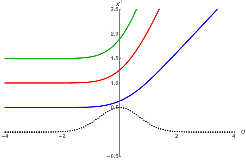
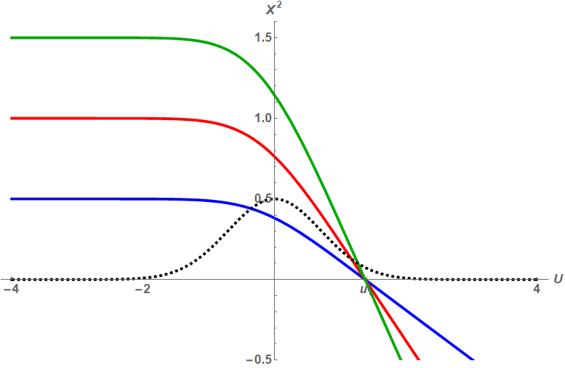
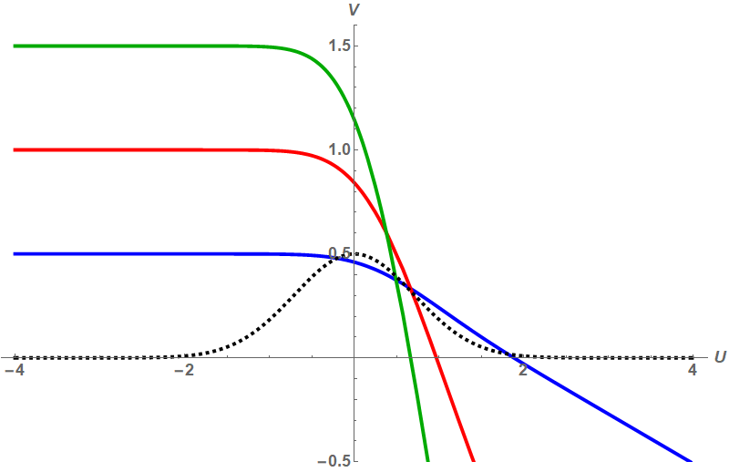
Figure 6: Geodesics in a Gaussian burst issued from various (blue/red/green)  initial rest positions in the Beforezone. By (IV.3) the effective force is repulsive in the $X^{1}$ coordinate and is attractive in that of $X^{2}$ where it focuses, for all initial positions at $(0,X_{0}^{2})$, at ${\mathbf{u}_{1}}=1.37653$. In the “far-After zone” i.e., beyond ${\mathbf{u}_{1}}$, the trajectories follow diverging straight lines.

The variation of the relative (euclidean) distance and the relative velocity,

$${\Delta}_{X}({\bf X},{\bf Y})=|{\bf X}-{\bf Y}|{\quad\text{\small and}\quad}{\Delta}_{\dot{X}}=|\dot{\bf X}-\dot{\bf Y}|,$$ (V.3)

shown in FIG.7 LongMemory are consistent with the velocity effect discussed in sec.IV.

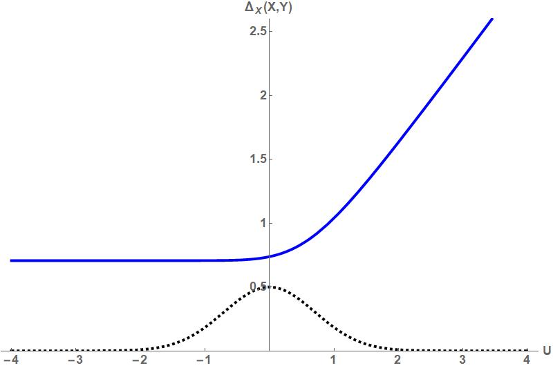
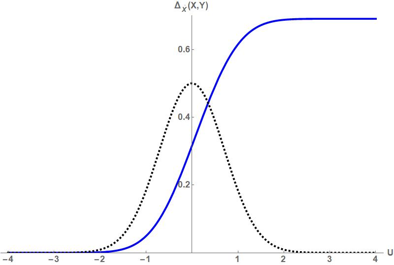
Figure 7: The relative velocity of particles initially at rest tend to a residual nonvanishing constant value after the wave has passed.

V.2 Linearly polarized sandwich wave, modelling flyby

In GibbHaw71 Gibbons and Hawking proposed to describe flyby by a Brinkmann profile proportional to first derivative of a Gaussian,

$${\mathcal{A}}_{\times}=0{\quad\text{\small and}\quad}{\mathcal{A}}(U)=\frac{1}{2}\,\frac{d(e^{-U^{2}})}{dU}\,.$$ (V.4)

​ ​

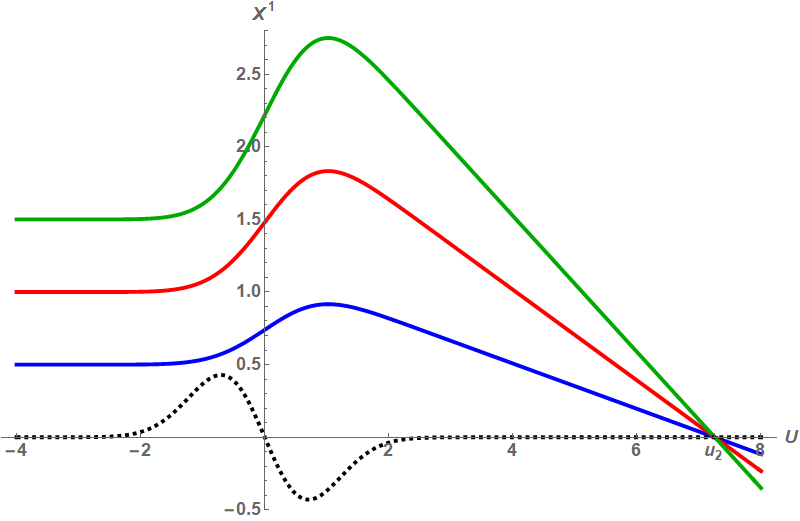
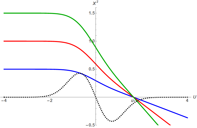
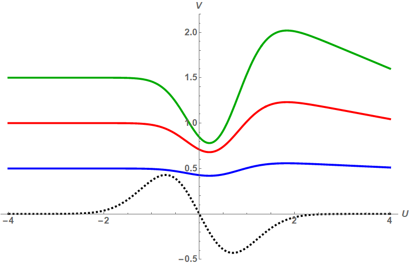
Figure 8: Evolution of geodesics with various resting positions for the flyby profile (V.4) proposed in GibbHaw71 shown in the background. The singular points where all components are focused are ${\bf u_{2}}=7.25437$ for $X^{1}$, and ${\bf u_{1}}=1.65034$ for $X^{2}$.

Further insight can be gained from the Tissot diagram Tissot : The evolution of (sorts of) “smoke rings” indicate the distorsion of a circle of particles which are at rest in the Beforezone due to the gravitational wave .

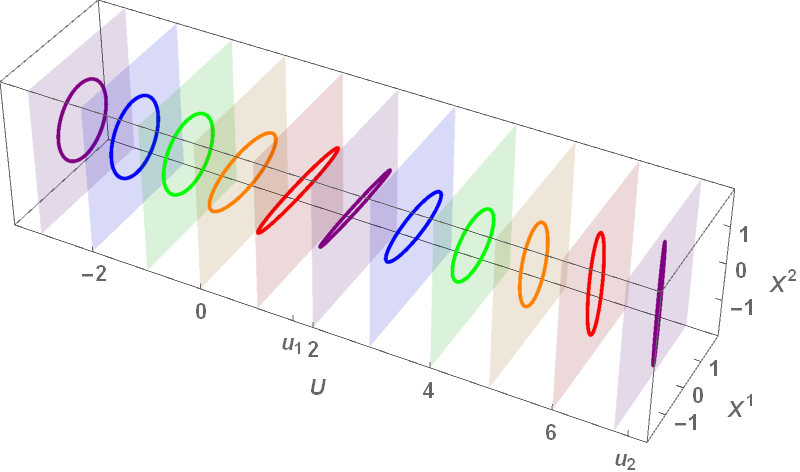
Figure 9: Tissot diagram for the flyby profile (V.4), to be compared with fig.8. The initial Tissot ring degenerates to a line segment at the values ${\bf u_{2}}$ and ${\bf u_{1}}$ where one or the other component vanishes.

The numerical results LongMemory ; Elbistan:2023pqb are reproduced in FIGs.8 and 9.

V.3 The Braginsky – Thorne system

The “burst with memory” scenario proposed by Braginsky and Thorne BraTho to observe gravitational waves has a linearly polarized profile which involves the second derivative of a Gaussian,

$${\mathcal{A}}_{+}(U)=\frac{1}{2}\,\frac{d^{2}(e^{-U^{2}})}{dU^{2}}\,.$$ (V.5)

The geodesics are depicted in FIG.10.

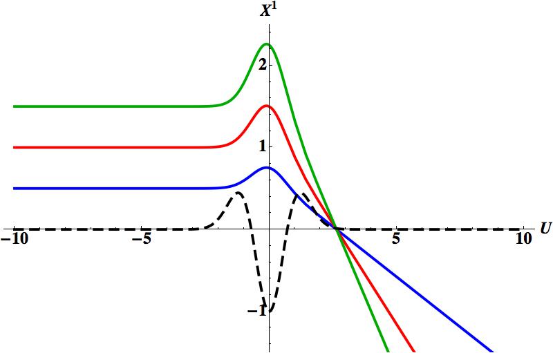
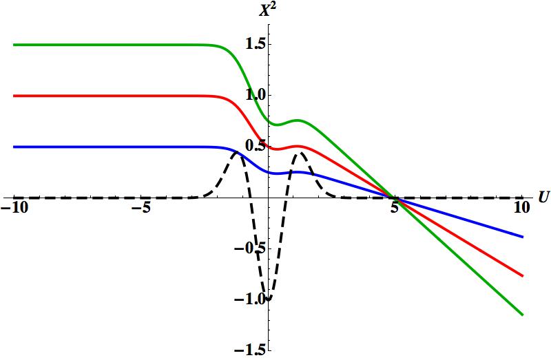
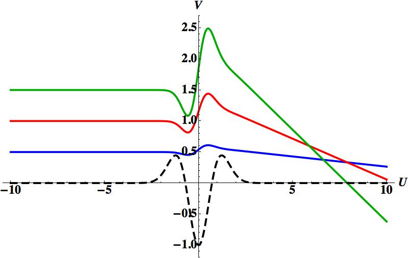
Figure 10: The burst with memory wave proposed by Thorne and Braginsky BraTho corresponds to the second derivative of a Gaussian, (V.5). All transverse components are focused, however at different points for the components.

V.4 Linearly polarized sandwich wave, modelling gravitational collapse

Next we focus our attention at the linearly polarized (approximate) sandwich wave, ${\mathcal{A}}_{\times}=0$, with Brinkmann profile (II.14) proposed in GibbHaw71 to model gravitational collapse, with profile

$${{\mathds{K}}}(U)={\mathcal{A}}(U)\mathrm{diag}(1,-1)\,,\qquad{\mathcal{A}}(U)=\frac{1}{2}\,\frac{d^{3}(e^{-U^{2}})}{dU^{3}}\,.$$ (V.6)

The numerical solution of the Brinkmann geodesic eqn. (IV.3) for the collapse profile proposed in GibbHaw71 is shown in FIG.11.

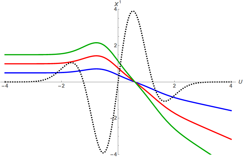
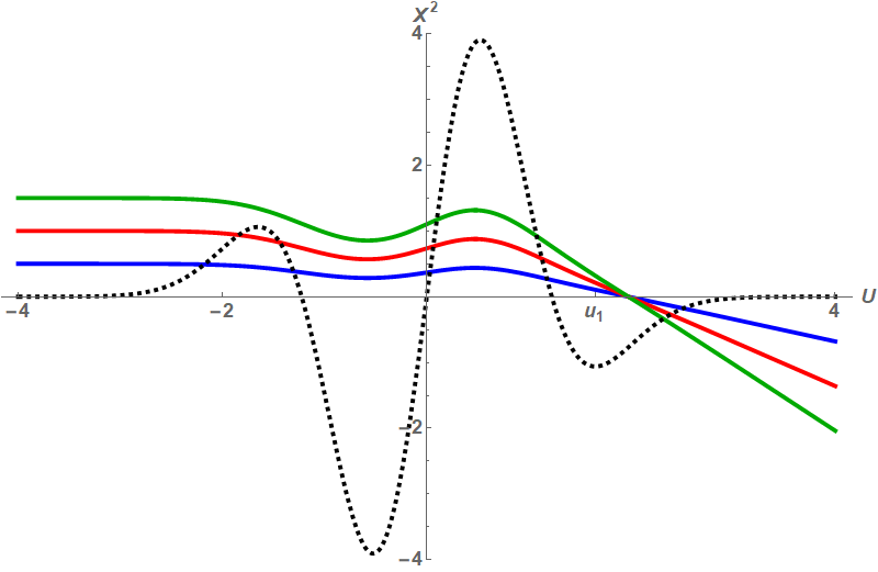
Figure 11: The special (Brinkmann) geodesics at rest at various (blue-red-green) positions in the Beforezone of the in the gravitational collapse wave GibbHaw71 , (V.6) (whose profile is dotted in the background). They converge where the effective potential in (IV.3) is attractive and diverge where it is repulsive. The components are focused for ${\bf u_{1}}=0.593342$ (resp. at ${\bf u_{2}}=1.97472$) which separate the regions where attraction turns into repulsion. In the flat Afterzone the motion is along straight lines with constant non-zero velocity.

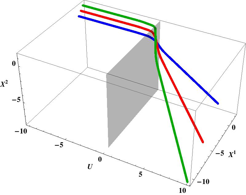
Figure 12: The trajectories in the gravitational collapse metric (V.6), unfolded to $(2+1)$D, diverge along straight lines in the Afterzone .

Consistently with (IV.11), all special geodesics ${\bf X}(u)$ whose initial position ${\bf X}_{0}$ belongs to the kernel of ${{\mathfrak{P}}}(u)$ are focused at a caustic point BoPi89 . This happens where $\det{{\mathfrak{P}}}(u_{i})=0,\,{i=1,2}$, or equivalently, where $\chi(u_{i})=0$. FIG.11 shows the focusing at $u_{1}$ (resp. at $u_{2}$) for the $X^{1}$ (resp. ($X^{2}$) component, cf. BoPi89 . Figs. 11 and 12 hint also at that the motions become again free in the flat Afterzone. From the Bargmann point of view Eisenhart ; DBKP ; DGH91 ; ZHAGK : the 4d geodesics project to those of a free non-relativistic particle in $(2+1)$d which moves consistently with Newton’s 1st law.

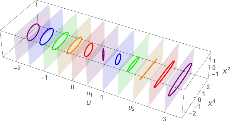
Figure 13: Tissot diagram for the linearly polarized sandwich wave (V.6). At the focal values ${\bf u_{1}}=0.593342$ and at ${\bf u_{2}}=1.97472$, respectively, the initial ring degerates to a vertical resp. horizontal segment, corresponding to the vanishing of one or the other column of the ${{\mathfrak{P}}}$-matrix.

In Brinkmann coordinates. Outside the (approximate) Wavezone the Brinkmann profile vanishes, ${{\mathds{K}}}\approx 0$, and the SL equation (II.16) reduces, in both the Before and the After zones, to the free equation,

$$\ddot{{\mathfrak{P}}}\approx 0{\quad\Rightarrow\quad}{\mathfrak{P}}(u)\approx\mathfrak{C}\,u+\mathfrak{D}\,{\quad\text{\small where}\quad}\mathfrak{C}=\mathrm{diag}(C_{1},C_{2})\,,\;\mathfrak{D}=\mathrm{diag}(D_{1},D_{2})$$ (V.7)

​with constants $C_{1},C_{2}$ and $D_{1},D_{2}$. Remember that, by (IV.11a), the columns of the ${{\mathfrak{P}}}$-matrix can also be viewed as particular geodesics, ${\bf X}_{1}(u)={\tiny\left(\begin{array}[]{c}P_{11}(u)\\ 0\end{array}\right)}$ and ${\bf X}_{2}(u)={\tiny\left(\begin{array}[]{c}0\\ P_{22}(u)\end{array}\right)}$. The initial conditions are cf. (II.22),

$$\left\{\begin{array}[]{llll}P_{11}(u_{0}^{B})=1,\quad P_{22}(u_{0}^{B})&=&1\\[4.0pt] \dot{P}_{11}(u_{0}^{B})=\>0,\quad\dot{P}_{22}(u_{0}^{B})&=&0\end{array}\right.\;{\;\;\text{\small for}\;\;}u_{0}^{B}<u_{B}\,,$$ (V.8)

in the Beforezone, implying that $C_{1}=C_{2}=0$ there. In the Afterzone we have instead,

$$\left\{\begin{array}[]{lll}P_{11}(u_{0}^{A})=D_{1}\,,\quad P_{22}(u_{0}^{A})&=&D_{2}\\[4.0pt] \dot{P}_{11}(u_{0}^{A})=C_{1}\,,\quad\dot{P}_{22}(u_{0}^{A})&=&\;C_{2}\end{array}\right.\;{\;\;\text{\small for}\;\;}u_{0}^{A}>u_{A}\,.$$ (V.9)

Thus

$${{\mathfrak{P}}}(u)=\mathrm{diag}(1,1) {\;\;\text{\small for}\;\;}u<u_{B}\,,$$ (V.10a)

$${{\mathfrak{P}}}(u)=\mathrm{diag}(C_{1}u+D_{1},C_{2}u+D_{2}) {\;\;\text{\small for}\;\;}u>u_{A}\,.$$ (V.10b)

BJR. The BJR matrix $\mathfrak{a}=(a_{ij})$ (II.1) is obtained by following the recipe of sec.II.2. By (V.7),

$$\mathfrak{a}={{\mathfrak{P}}}^{2}=\left\{\begin{array}[]{cll}\mathrm{diag}(1,1)&\quad\text{in Beforezone}&u<u_{B}\\[6.0pt] \mathrm{diag}\Big{(}(C_{1}u+D_{1})^{2},(C_{2}u+D_{2})^{2}\Big{)}&\quad\text{in Afterzone}&u_{A}<u\end{array}\right.\;,$$ (V.11)

shown in FIG.14.

By (IV.8) the trajectories in BJR coordinates are determined by the conserved quantities ${\bm{p}}$ and $\mathbf{k}$, and by the Souriau matrix ${{\mathfrak{S}}}$ in (III.2).

The determinant (II.10) satisfies the Sturm-Liouville equation (II.11), whose behavior depends on the frequency $\omega(u)$, depicted in FIG.15. The determinants $\det{({\mathfrak{P}})}$ and $\det({\mathfrak{a}})$ vanish when either $P_{11}$ or $P_{22}$ does, i.e., at ${\mathbf{u}_{1}}$ and ${\mathbf{u}_{2}}$, respectively.

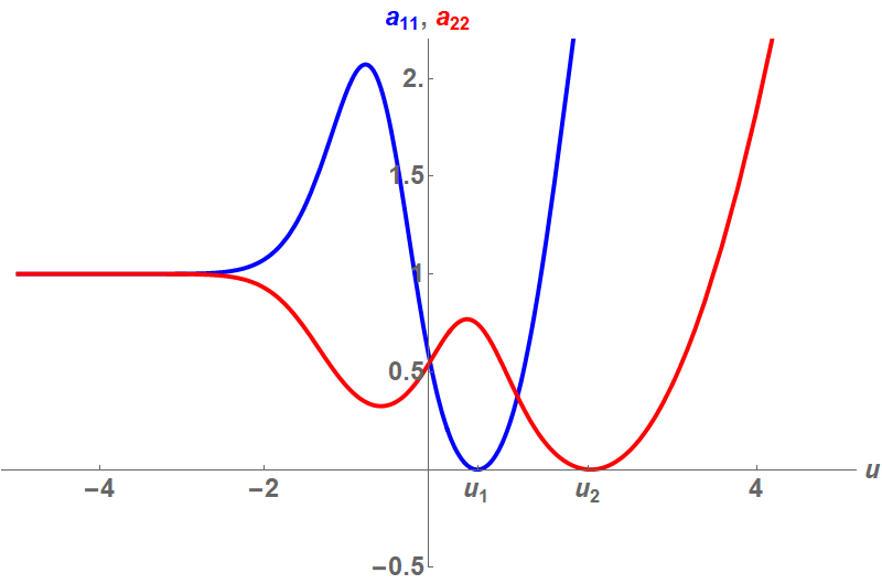
Figure 14: The BJR profile $\mathfrak{a}=(a_{ij})$ of the collapse wave, whose Brinkmann profile is (V.6). $a_{11}$ = $a_{22}$ $=1$ in the Beforezone. The zeros ${\mathbf{u}_{i}},i=1,2$ are where one or the other component vanishes (and where the Tissot ring degenerates to a segment, cf. FIG.13).

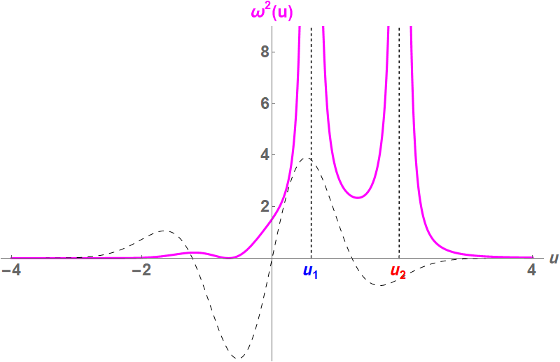
Figure 15: In BJR, the frequency ${\bm{\omega}}$ in the Sturm-Liouville equation (II.11) for the linearly polarized collapse wave (with Brinkmann profile (V.6) of GibbHaw71 shown in the background) diverges at the points ${\bf u_{i}},i=1,2$ where the determinant of the metric vanishes, $\chi(u_{i})$.

From eqn (II.11) we infer that to keep $\ddot{\chi}$ finite the frequency $\omega$ must diverge to infinity at a zero of the determinant, $\lim_{u\to u_{i}}\omega=\infty$ when $\chi(u_{i})=0,\,i=1,2$. Outside the Wavezone the frequency $\omega$ is approximately zero and the SL eqn (II.11) reduces to $\ddot{\chi}\approx 0$, implying that $\chi$ is approximately linear,

$$\chi\approx cu+d\,.$$ (V.12)

The condition $c=0$ in the Beforezone changes to $c\neq 0$ in the Afterzone, due precisely to the wave. Therefore $\chi$ vanishes there at most once, consistently with FIGs.15 and 16.

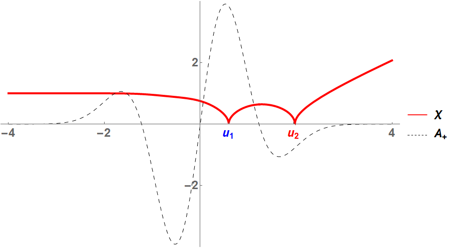
Figure 16: ${\bm{\chi}}=(\det(\mathfrak{a}))^{1/4}$ for the linearly polarized “collapse” wave (V.6). The zeros of ${\bm{\chi}}$ coincide with the points ${\bf u_{i}},\,i=1,2$, where the Brinkmann trajectories are focused, and also where the frequency ${\bm{\omega}}$ diverges, cf. (FIG.15). In the flat Outside regions ${\bm{\chi}}$ is approximately linear.

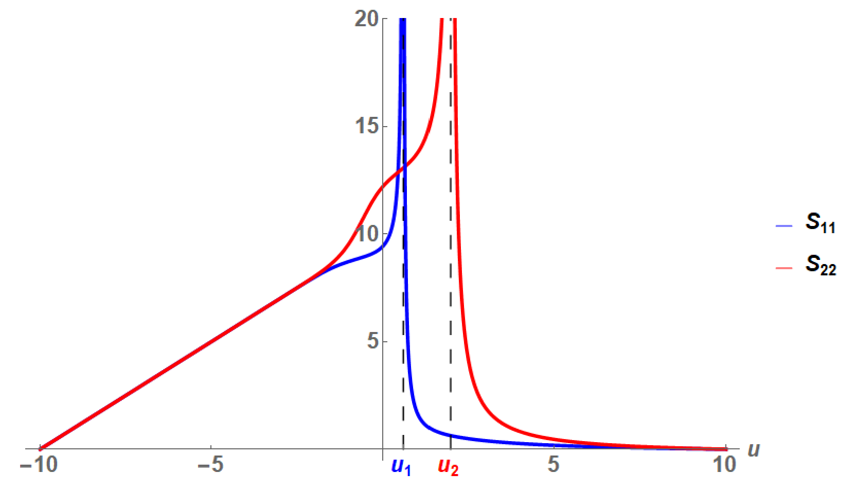
Figure 17: The Souriau matrix ${{\mathfrak{S}}}$ (III.2) provides us, in BJR coordinates, both with the geodesics (IV.8) and also with (distorted) boosts, implemented as in (III.8). ${{\mathfrak{S}}}(u)\approx u{\,}\mathds{I}$ in the Beforezone, then diverges at ${\mathbf{u}_{1}}$ and at ${\mathbf{u}_{2}}$ and falls off rapidly in the Afterzone.

The behavior of the Souriau matrix we read off FIG.17 has remarkable consequences. In the Beforezone, it behaves as in the Minkowski/Galilei case, but in the Afterzone ${{\mathfrak{S}}}\approx 0$, and (IV.8) reduces to

$${\bf x}\approx\mathbf{k}=\mathop{\rm const.}\nolimits\qquad v(u)\approx e\,u+v_{0}\,,$$ (V.13)

so that the geodesic is “vertical”. The transverse coordinates are fixed, confirming that in BJR coordinates “Carroll particles do not move” [in transverse space].

Figure 18: In a linearly polarized “gravitational collapse wave” (V.6) the numerically found Brinkmann trajectories in the flat Afterzone are straight lines, which overlap perfectly with those obtained in BJR coordinates and then carried to Brinkmann by (II.18).

FIG.18 confirms that carrying the BJR solutions to Brinkmann by the map (II.18) removes the divergences. The pieces fit together and we end up with the same regular curve obtained before numerically SLC ; ZCEH ; ShortMemory .

Distorted Carroll symmetry. According to (III.8), a boost with parameter ${\mathbf{b}}$ acts, in BJR coordinates, as,

$${\bf x}\to{\bf x}+{{\mathfrak{S}}}(u)\,{\mathbf{b}}\,$$ (V.14)

where ${{\mathfrak{S}}}(u)$ is the Souriau matrix (III.2). Expressed in Brinkmann coordinates, this becomes (III.10)  i.e.,

$${\bf X}\to{\bf X}+{{\widetilde{\mathfrak{P}}}}(u){\mathbf{b}}\,,{\quad\text{\small where}\quad}{{\widetilde{\mathfrak{P}}}}(u)={{\mathfrak{P}}}(u){{\mathfrak{S}}}(u)\,.$$ (V.15)

$\bullet$ For a special geodesic in particular, $\mathfrak{a}={{\mathfrak{P}}}^{2}=\mathds{I}$ in the Beforezone and the Souriau matrix is simply ${{\mathfrak{S}}}(u)=(u-u_{0})\mathds{I}{\;\;\text{\small for}\;\;}u,u_{0}<u_{B}\,.$ The usual free (Galilean) implementation is thus we recover

$${{\widetilde{\mathfrak{P}}}}=(u-u_{0})\,\mathds{I}\,{\;\;\text{\small for}\;\;}u<u_{B}\,.$$ (V.16)

$\bullet$ In the Afterzone the Souriau matrix ${{\mathfrak{S}}}=\mathrm{diag}(S_{11},S_{22})$ can be calculated by using $\mathfrak{a}$ in (V.11),

$$S_{11}=\frac{1}{C_{1}(C_{1}u+D_{1})}{\quad\text{\small and}\quad}S_{22}=\frac{1}{C_{2}(C_{2}u+D_{2})}\,\;{\;\;\text{\small for}\;\;}u_{A}<u\,.$$ (V.17)

Combining with (V.7) we find that in the Afterzone ${{\widetilde{\mathfrak{P}}}}={{\mathfrak{P}}}{{\mathfrak{S}}}$ is an (approximately) constant diagonal matrix,

$${{\widetilde{\mathfrak{P}}}}={{\mathfrak{P}}}{{\mathfrak{S}}}\approx-\,\mathrm{diag}(\frac{1}{C_{1}},\frac{1}{C_{2}})\,\;{\;\;\text{\small for}\;\;}u_{A}<u\,.$$ (V.18)

Thus, as confirmed numerically in FIG.19, boosts act in the far-right Afterzone as (generically anisotropic) translations,

$${\bf X}\to{\bf X}+\,\big{(}\frac{b_{1}}{C_{1}},\frac{b_{2}}{C_{2}}\big{)}\,.$$ (V.19)

Outside the Wavezone our results are consistent with the numerical ones shown in FIG.19.

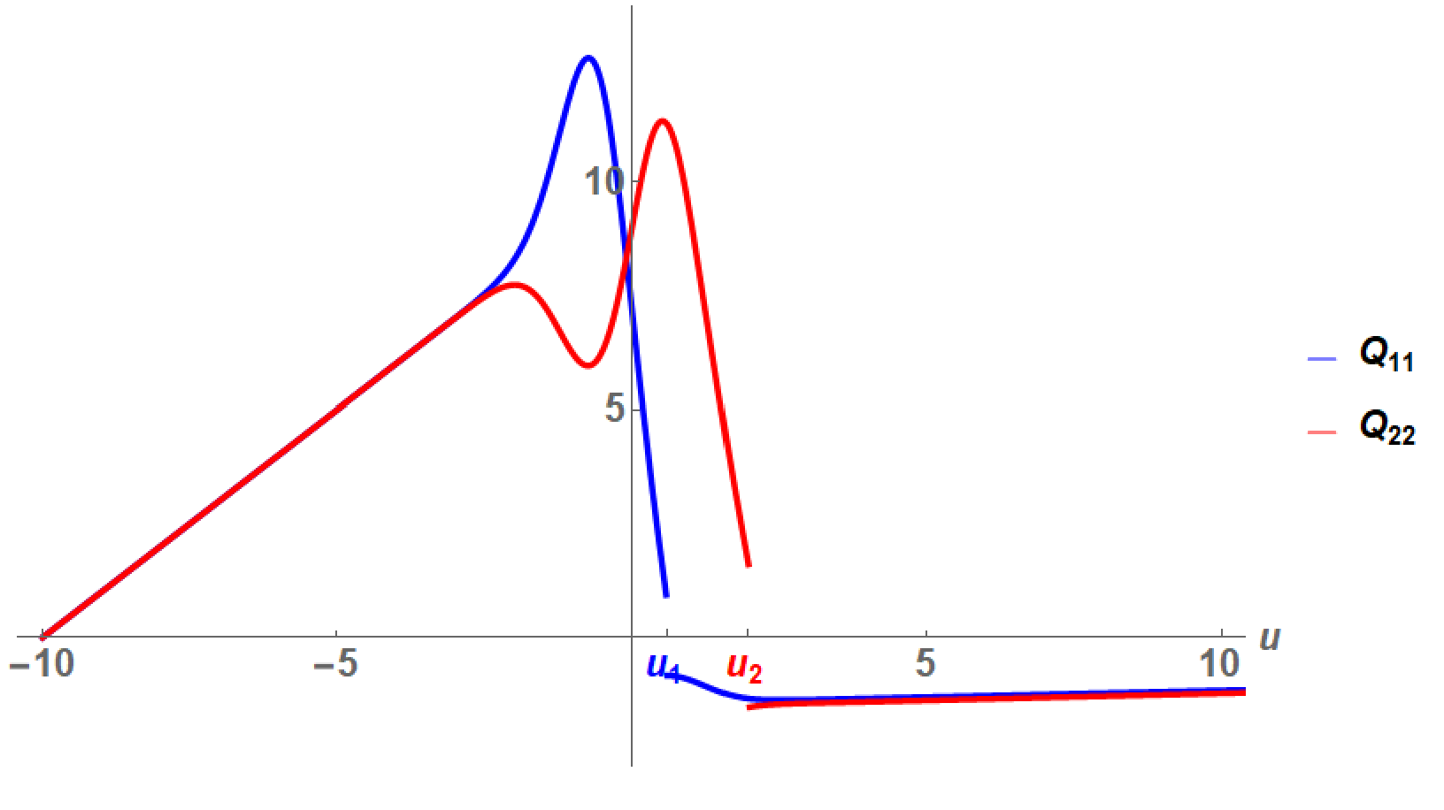
Figure 19: The matrix ${{\widetilde{\mathfrak{P}}}}={{\mathfrak{P}}}{{\mathfrak{S}}}$ reduces to the usual Galilean expression in the Beforezone but is approximately a constant matrix, (V.18), in the Afterzone. At the singular points $u_{i}$ where the ${{\mathfrak{P}}}$ and $\mathfrak{a}$ matrices vanish so that the Souriau matrix ${{\mathfrak{S}}}$ diverges we have a numerical uncertainty.

Translations,

$${\bf x}\to{\bf x}+{\mathbf{c}}\,,$$ (V.20)

which are manifest symmetries of the BJR metric (II.1), behave in the opposite way. In Brinkmann coordinates they are implemented as

$${\bf X}\to{\bf X}+{{\mathfrak{P}}}(u)\,{\mathbf{c}}\,.$$ (V.21)

Thus while they are usual translations in the Beforezone where ${{\mathfrak{P}}}(u)=\mathds{I}$, in the Afterzone we find, by (V.10b),

$${\bf X}\to{\bf X}+\mathrm{diag}\Big{(}C_{1}u+D_{1})c_{1},(C_{2}u+D_{2})c_{2}\Big{)}\,.$$ (V.22)

V.5 Circularly polarized sandwich waves

As yet another illustration, we study a circularly polarized (approximate) sandwich wave, (II.14), with PolPer ; SLC ,

$${\mathcal{A}_{+}}(U)=\frac{\lambda}{\sqrt{\pi}}\,e^{-\lambda^{2}U^{2}}\cos(\Omega U){\color[rgb]{1,0,0}\,},\qquad{\mathcal{A}_{\times}}(U)=\frac{\lambda}{\sqrt{\pi}}\,e^{-\lambda^{2}U^{2}}\sin(\Omega U)\,.$$ (V.23)

depicted in FIG.20. We shall choose $\lambda=0.1$ and $\Omega=\sqrt{2}$. The behavior for various (small and large) values of $\lambda$ is studied in PolPer .

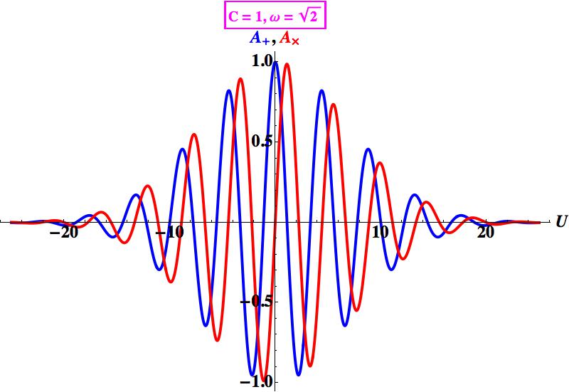
Figure 20: Circularly polarized (approximate) sandwich wave in Brinkmann coordinates with Gaussian envelope, (V.23). The colors refer to the $\bf{{\color[rgb]{0,0,1}\mathcal{A}_{+}}}$ and the ${\mathcal{A}_{\times}}$ polarisation components.

The metric in Brinkmann coordinates is perfectly regular for all $U$. The BJR coordinates given by (II.18) are instead defined only in coordinate patches between adjacent zeros of the determinant of ${{\mathfrak{P}}}$ (or of $\mathfrak{a}$), plotted in FIG.21.

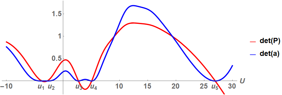
Figure 21: The BJR coordinates are well-defined only between between adjacent zeros $\mathbf{u_{i}}$ of the determinant of the BJR profile, ${\color[rgb]{0,0,1}{\mathbf{\chi}^{4}}=\det(\mathfrak{a})}>0$ or equivalently, the zeros of ${\mathbf{\det}({{\mathfrak{P}}})}$ : $\mathbf{u_{1}}\approx-3.75,\,\mathbf{u_{2}}\approx-2.80,\,\mathbf{u_{3}}\approx 2.74,\,\mathbf{u_{4}}\approx 5.09,\,\mathbf{u_{5}}\approx 26.97$, where the BJR coordinates become singular. $\det(\mathfrak{a})\approx 1$ in the Beforezone (far left), and then steadily increasing in the Afterzone (on the far right). The 5 zeros of $det({{\mathfrak{P}}})$ are $U=-3.75,-2.80,2.74,5.09,26.97$ therefore 6 patches are necessary to cover the entire $u$-axis.

The entries of the matrix ${{\mathfrak{P}}}=(P_{ij})$, obtained by solving numerically the Sturm-Liouville equation (II.16) are shown in FIG.22.

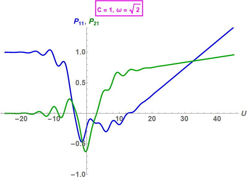
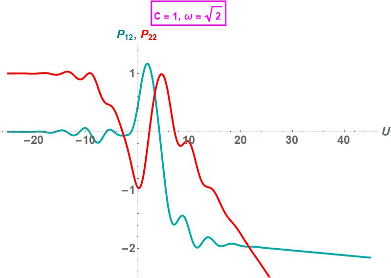
(a)                                                                    (b)

Figure 22: The ${{\mathfrak{P}}}$-matrix is obtained by solving (numerically) the Sturm-Liouville eqn. (II.16). ${\color[rgb]{0,0.35,0}\bf{P}_{21}}$, and ${\color[rgb]{0,1,1}\bf{P}_{21}}$ and ${\color[rgb]{1,0,0}\bf{P}_{22}}$ can also be viewed as components of special geodesics for particular choices of initial position.

The BJR profile $\mathfrak{a}=\big{(}a_{ij}\big{)}$ (II.17) deduced from the ${{\mathfrak{P}}}$-matrix is shown FIG.23.

Figure 23: The BJR profile of the gravitational wave (II.14)-(V.23) is given by a symmetric matrix ${\bf a}=\big{(}a_{ij}\big{)}={{\mathfrak{P}}}^{\dagger}{{\mathfrak{P}}}$.

Special geodesics. The two columns of the ${{\mathfrak{P}}}$-matrix unfolded to (2+1)d,

$$\hat{{\bf X}}^{(1)}(U)=\left[\small{\left(\begin{array}[]{c}P_{11}(U)\\ P_{21}(U)\end{array}\right)},U\right]{\quad\text{\small and}\quad}\hat{{\bf X}}^{(2)}(U)=\left[\small{\left(\begin{array}[]{c}P_{21}(U)\\ P_{22}(U)\end{array}\right)},U\right]\,,$$ (V.24)

($U=u$) are special Brinkmann-form geodesics at rest for $u_{0}<u_{B}$ at

$${\bf X}^{(1)}_{0}={\small{\left(\begin{array}[]{c}{\color[rgb]{0,0,1}\bf 1}\\ {\color[rgb]{0,0.35,0}\bf 0}\end{array}\right)}}{\quad\text{\small and}\quad}{\bf X}^{(2)}_{0}={\small{\left(\begin{array}[]{c}{\color[rgb]{0,1,1}\bf 0}\\ {\color[rgb]{1,0,0}\bf 1}\end{array}\right)}}\,,$$ (V.25)

respectively. FIGs.22 - 25 show that the complicated motions in the Wavezone are straightened out in the Afterzone, consistently with the Bargmann interpretation. Tissot’s indicatrix is plotted in FIG.26.

Figure 24: In Brinkmann coordinates, the trajectory components $X^{1}(u)$, $X^{2}(u)$ of a special geodesic [which is at rest in the Beforezone], ${\bf X}_{0}=({\color[rgb]{0,0,1}\bf 1},{\color[rgb]{1,0,0}\bf 1})$, become straight lines in the Afterzone, as illustrated on the example of a circularly polarized sandwich wave.

      (a)                                                                           (b)

Figure 25: Brinkmann trajectories for initial conditions ${\bf X}^{(1)}_{0}=(0,1)$ and ${\bf X}^{(2)}_{0}=(1,0)$ in (V.25). (a) unfolded to $2+1$ dimensions. (b) Projected to the transverse plane. The complicated motions in the Wavezone are smoothed out in the Afterzone where they follow straight trajectories with constant non-zero velocities.

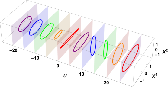
Figure 26: Tissot diagram for a circularly polarized sandwich wave (V.23) shown in FIG.20.

Symmetries. Distorted boosts (III.8) are expressed by using the Souriau matrix ${{\mathfrak{S}}}$ in (III.2). Combining our previous results allows us to plot them in BJR coordinates, (FIG.27). The implementation in the Afterzone differs substantially from the Galilean one.

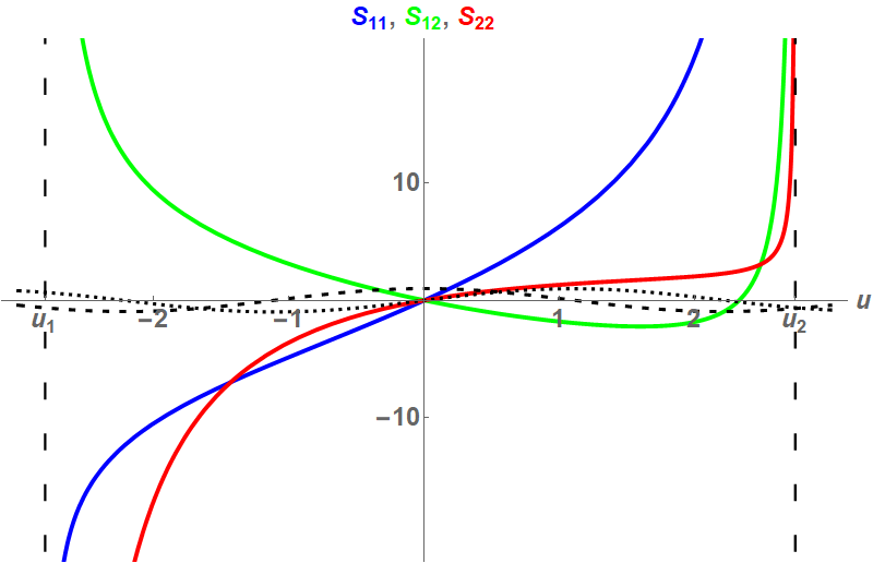
Figure 27: In BJR coordinates, boosts are implemented through the Souriau matrix ${{\mathfrak{S}}}$ as in (III.8). We took ${\mathbf{b}}=(1,1)$. The dotted and dashed lines in the background indicate the ${\mathcal{A}}_{+}$ and ${\mathcal{A}}_{\times}$ components of the Brinkmann profile (II.14). ${{\mathfrak{S}}}$ is defined between two subsequent zeros $\mathbf{u_{k}}$ and $\mathbf{u_{k+1}}$ of the $\mathfrak{a}$ (or $P$)-matrix (see FIG.21). Our plot shows what happens in $[-3,3]$ which contains $I_{2}=\big{[}\mathbf{u_{2}},\mathbf{u_{3}}\big{]}$ where $\mathbf{u_{2}}\approx-2.8$ and $\mathbf{u_{3}}\approx 2.7$ are the singular points which are the closest to the origin. $I_{2}$ contains the Wavezone. All components of the Souriau matrix  ${\mathfrak{S}}$ manifestly diverge when $u\to\mathbf{u_{i}},i=2,3$.

Covering the $u$-axis with BJR domains and gluing together the results in the subsequent coordinate patches yields the complicated figure FIG.28, obtained by calculating the integrals $\displaystyle\int_{u_{0}}^{u}\!\!a^{-1}$ for $u_{0}\equiv{u_{0}}^{(k)},\,u\in I_{k}$. In detail, we calculated numerically

1. on the left-hand part, for $u_{0}^{(1)}=-20,\,u<3$ (which lies in the Beforezone),

2. in middle part, with $u_{0}^{(2)}=0,\,-3<u<3$ (which contains the Wavezone),

3. in the right-hand part, for $u_{0}^{(3)}=3<u<20$, (which lies in the Afterzone).

Glueing the results obtained in the intervals $I_{k}$, (FIG.28) indicates that at the contact points $u_{k}$ the Souriau matrix diverges from both sides.

 

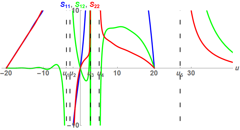
Figure 28: The implementation of a boost through the Souriau matrix is essentially Galilean in the Beforezone $u<u_{B}$ but differs substantially from the latter both in the Wavezone and in the Afterzone.

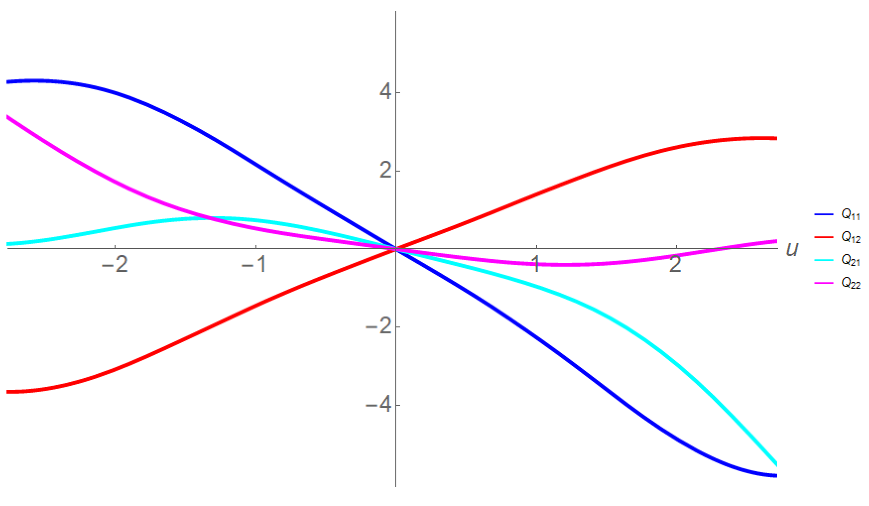
Figure 29: The ${{\widetilde{\mathfrak{P}}}}={{\mathfrak{P}}}{{\mathfrak{S}}}$-matrix (III.11) which implements boosts in Brinkmann coordinates, (III.10), plotted in $[-3,3]$ as in FIG.27. To be compared with FIG.19.

VI Connecting the Before and Afterzones

In both flat regions the motion is free, determined by the constant velocity, $c$ in (II.12). For our special geodesics $c=0$ in the Beforezone, but it is some different, nonzero constant in the Afterzone. The two separated flat zones are connected through the Wavezone, though, where the sandwich profile and therefore the motions are nontrivial and can indeed by quite complicated as seen in FIGs. 22-25.

The velocity in the Afterzone is then determined by the integrals (IV.5). Since the Sturm-Liouville equation can not be solved analytically in general, we have to resort to numerical calculation: first one determines the trajectories (the initial position where chosen $X^{1}(-\infty)=1$ and $X^{2}(-\infty)=2$). Then insertion into (IV.5) yields the velocities, see FIGs. 30-31-32-33.

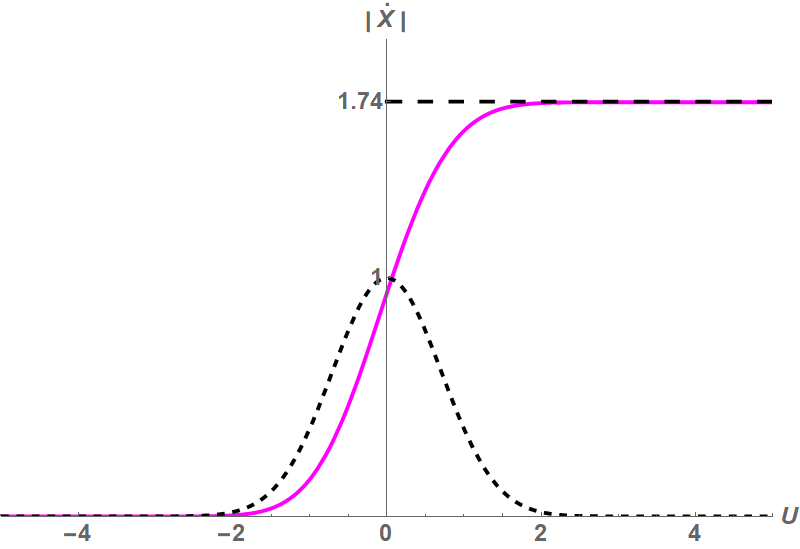
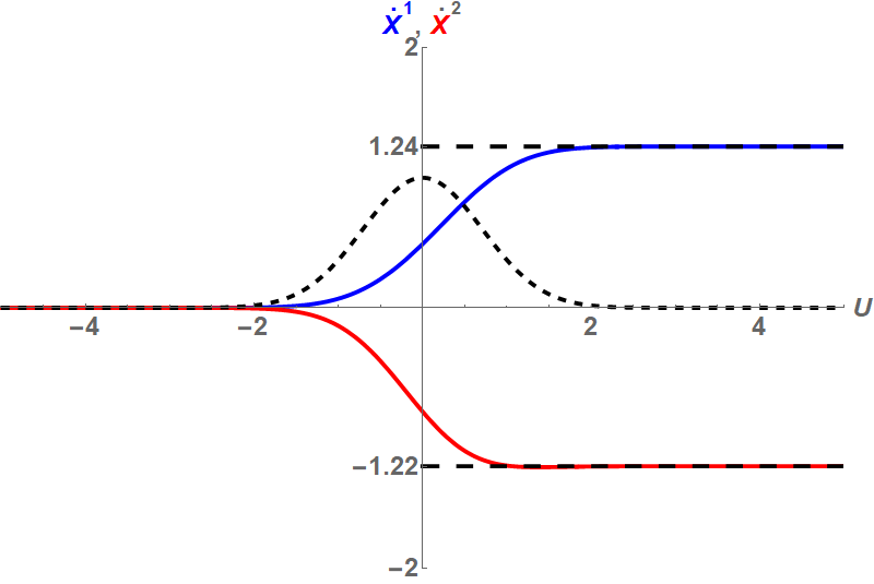
Figure 30: Velocity jump between the flat Before and Afterzones for the simple Gaussian profile (V.1).

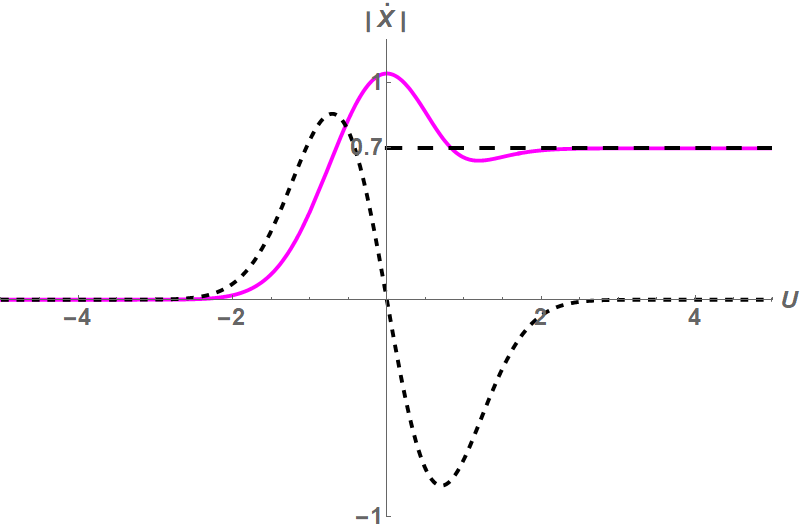
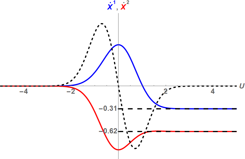
Figure 31: Velocity jump for the first derivative of the Gaussian, (V.4), representing flyby.

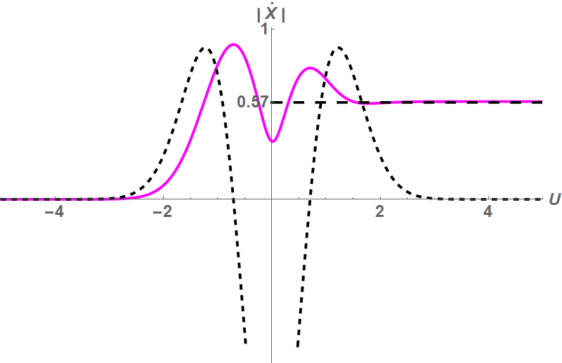
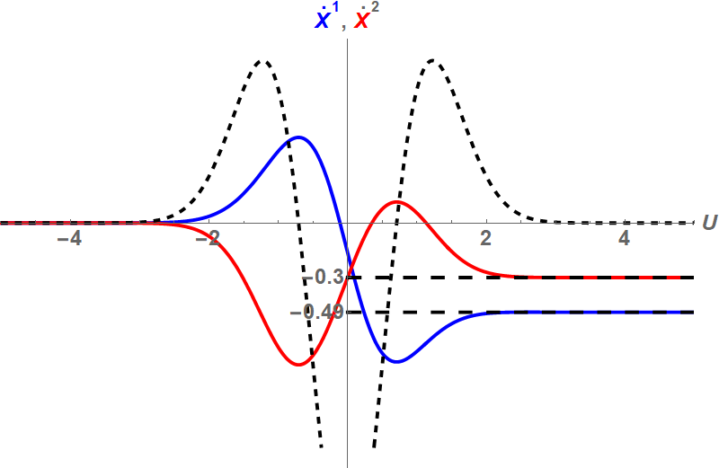
Figure 32: Velocity jump for the second derivative of the Gaussian, (V.5), FIG.10, proposed by Braginski and Thorn.

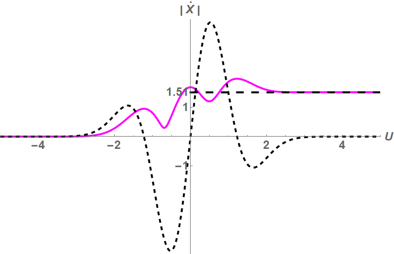
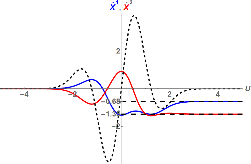
Figure 33: Velocity jump for the third- derivative-of-the-Gaussian profile, (V.6) in FIG.11, proposed for gravitational collapse GibbHaw71 .

VII Impulsive limit

The impulsive (or shock-wave) limit leads to subtle analytic questions Penr2 ; Steinbauer:1997dw ; Kunzinger:1998nz ; BarHog ; PodSB ; Podolsky:2022ase , and to some controversy ImpMemory ; SBComment . A rigourous study goes beyond our scope here, therefore we limit ourselves with a couple of intuitive statements. In fact, we discuss only one simple example, namely that of the linearly polarized Gaussian profile (V.1) with a scale factor $\lambda$,

$${\cal A}(U)=\frac{\lambda}{\sqrt{\pi}}\,e^{-\lambda^{2}u^{2}}\,.$$ (VII.1)

Squeezing the profile by letting $\lambda\to\infty$ yields the impulsive profile shown in Fig.34 ,

$${\mathcal{A}}\equiv{\mathcal{A}}_{+}(U)=2k\,\delta(U)\,.$$ (VII.2)

Conversely, $k$ is recovered as

$$k=\frac{1}{2}\int_{-\infty}^{+\infty}\!\!{\mathcal{A}}(U)dU\,.$$ (VII.3)

In our FIGs.22 - 25 we have choosen $k=\frac{1}{2}$.

Taking the $\lambda\to\infty$ limit of the damped Gaussian profile (VII.1) in FIGs.34, the ${\mathfrak{P}}$-matrix of an impulsive wave breaks between the Before and the Afterzones by ImpMemory ,

$$\Delta\dot{{\mathfrak{P}}}\equiv\dot{{\mathfrak{P}}}(0+)=\mathfrak{c}_{0}\,.$$ (VII.4)

But for a linearly polarized wave the ${\mathfrak{P}}$-matrix is also a trajectory, so this implies a velocity jump,

$$\;\;\displaystyle{\dot{{\bf X}}(0+)=\mathfrak{c}_{0}\,{\bf X}_{0}\,.}\;\;$$ (VII.5)

The memory effect in an impulsive gravitational wave can also be studied in BJR coordinates. The reader is referred to ImpMemory ; SBComment for details.

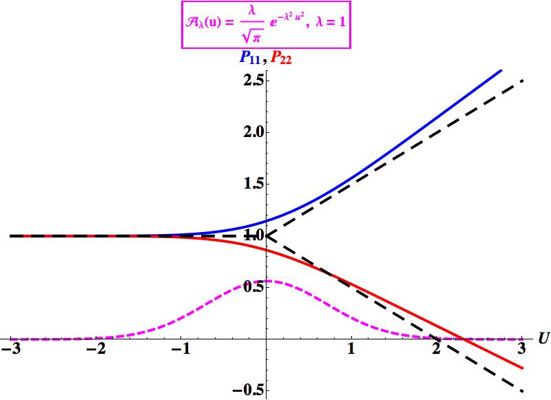
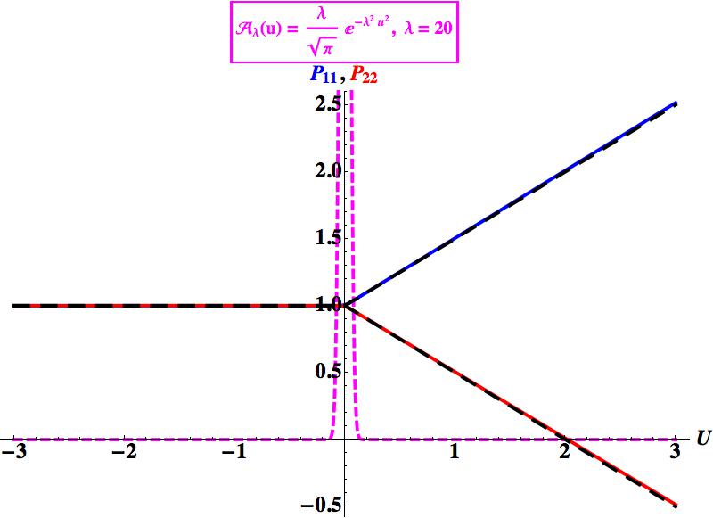
(a)                                                               (b).

Figure 34: The matrix ${\mathfrak{P}}(u)=\mathrm{diag}\big{(}P_{11}(u),P_{22}(u)\big{)}$ [alias special geodesic] for the linearly polarized Brinkmann profile of the form (V.1), i.e., ${\cal A}(U)=(\lambda/\sqrt{\pi})e^{-\lambda^{2}u^{2}}$ with $\lambda=1\,,20\,$. When $\lambda\to\infty$ the profile tends to that of an impulsive wave, (VII.2). The numerical solutions are plotted in solid blue and red lines. For large $\lambda$, ${\mathfrak{P}}$ tends to the analytic impulsive profile depicted in dashed black lines. The solution is regular for $u<k^{-1}=u_{0}$, which is also a zero of $\det(\chi)$.

Figure 35: For small $\lambda$, de behavior is substantially different from that in the impulsive ($\lambda\to\infty)$ case.

VIII Conclusion

Gravitational waves could, in principle, be observed also through the Memory Effect. In the ‘standard’ version called the displacement effect (DM) proposed by Zel’dovich-Polnarev and their collaborators ZelPol ; BraTho ; BraGri the particles initially at rest will have an approximately vanishing relative velocity Christo .

Another version (to which our paper is devoted), was proposed, earlier, by Ehlers and Kundt Ehlers , and by Souriau Sou73 , finds instead that the particles move, after the passing of a burst of a plane gravitational wave, with constant but non-zero velocity Sou73 ; BraGri ; BoPi89 ) and is called therefore velocity effect (VM).

Souriau Sou73 found, in particular, that using Baldwin-Jeffery-Rosen (BJR) coordinates BaJeRo makes the description straightforward, eqn. (IV.8), – but the price to pay for it is that the coordinates are only local: the become necessarily singular and the solutions obtained in adjacent intervals have to be glued together. In the linearly polarized “collapse” case (sect.V.4), for example, we need 3 patches, and for the circularly polarized one (sect.V.5) we need 6 patches .

The question of symmetries is even more subtle. It has long been known that the gravitational wave metric admits generically a 5-parameter isometry group BoPiRo ; exactsol . Three of them are obvious (translations), however two of them could be identified only as solutions of a Sturm-Liouville equation Torre ; SLC .

Souriau Sou73 , who followed his own ideas [as he always did], found an elegant explicit expression in BJR coordinates, (III.8), in terms of the matrix ${\mathfrak{S}}$ in (III.2) which allow us to identify the symmetry as Lévy-Leblond’s Carroll symmetry with broken rotations Leblond ; Carroll4GW (what Souriau did not recognize). We just mention that the difference between the two, (displacement and velocity) types effects might well be related to the double Carroll structure, one associated with BMS BMS ; Sachs61 ; Sachs62 ; ConfCarrBMS ; PeHaStPRL ; PeHaSt1611 , and the other with the internal dipole symmetry of fractons considered in condensed matter physics Bidussi ; LD ; Figueroa and references in them. Further applications of the Carroll symmetry include the cosmic Hall effect Marsot ; HallonHole .

Souriau’s expression can be pulled back to global Brinkmann coordinates. However:

$\bullet$ The solutions found in BJR coordinates are valid only in coordinate patches and requires us “to glue them together”;

$\bullet$ Their transcription to global Brinkmann coordinates requires to solve a Sturm-Liouville equation;

$\bullet$ Solving the equations of motion directly in Brinkmann coordinates leads to similar difficulties: it requires in particular to solve another Sturm-Liouville equation SLC . Analytical solutions are therefore exceptional and one has to resort to numerical work Carroll4GW ; SLC ; Elbistan:2022plu .

The BJR solutions diverge at the contact points of the adjacent intervals. FIG.27 and FIG.29 indicate, however, that multiplication by ${\mathfrak{P}}$, (II.21), regularizes the trajectories. Accordingly, the ${\widetilde{\mathfrak{P}}}={\mathfrak{P}}{\mathfrak{S}}$ matrix yields smooth (although unusual) implementations of the boosts.

Impulsive waves whose wave-zone is so narrow that it can be approximated by a Dirac delta yield explicit analytic solutions. Unphysical as it might appear at first, the impulsive approximation is indeed quite realistic: think at those gravitational waves which, after having travelled at the speed of light for thousands or even millions of years, cross through the earth in a fraction of a second.

To conclude, our review is admittedly “strip-cartoon-like”. We would however recall a poem written by the author of Alice entitled “The Ocean Chart” Snark :

[the Captain] …had bought a large map representing the sea,
Without the least vestige of land:
And the crew were much pleased when they found it to be
A map they could all understand.

Appendix A The Bargmann framework

Eisenhart Eisenhart has shown that the dynamics of a conservative holonomic dynamical system with $n$ degrees of freedom can be transcribed as geodesic motion in a certain Lorentzian space-time of dimension $n+1$. He starts with the space-time Lagrangian

$$L=\frac{1}{2}\,\mathrm{g}_{\alpha\beta}\,\dot{x}^{\alpha}\dot{x}^{\beta}-V$$ (A.1)

with coordinates $(x^{\alpha})=(x^{1},\ldots,x^{n},x^{n+1})$, where $t=x^{n+1}$ stands for the absolute time-coordinate; the quadratic form $(\mathrm{g}_{\alpha\beta})$ as well as the potential function $V$ depend arbitrarily upon $(x^{\alpha})$. The quadratic form $(\mathrm{g}_{\alpha\beta})$ is not assumed to be non-degenerate as usual in non-relativistic mechanics, however the sub-matrix $(\mathrm{g}_{ij})$ where $i,j=1,\ldots,n$ is required to represent locally a Riemannian metric on each time-slice $t=\mathop{\rm const.}\nolimits$.

Rewriting the Lagrangian (A.1) as

$$L=\frac{1}{2}\,\mathrm{g}_{ij}\,\dot{x}^{i}\dot{x}^{j}+A_{i}\dot{x}^{i}+\frac{1}{2}\mathrm{g}_{tt}-V,$$ (A.2)

where $A_{i}=\mathrm{g}_{it}$, we end up with the Lagrange equations

$$\mathrm{g}_{ij}\ddot{x}^{i}+\Gamma_{jki}\,\dot{x}^{j}\dot{x}^{k}+\big{(}\partial_{t}\mathrm{g}_{ij}+\partial_{i}A_{j}-\partial_{j}A_{i}\big{)}\dot{x}^{j}+\partial_{t}A_{i}+\partial_{i}\big{(}-\frac{1}{2}\mathrm{g}_{tt}+V\big{)}=0$$ (A.3)

for all $i=1,\ldots,n$, where the $\Gamma_{jki}$ denote the Christoffel symbols of the metric $(\mathrm{g}_{ij})$ of a $t=\mathop{\rm const.}\nolimits$ slice. The equations (A.3) can be viewed as the geodesic equations of a special Lorentz metric on an $(n+2)$ dimensional extended space-time with coordinates $(x^{\mu})=(x^{1},\ldots,x^{n},t,s)$ where $s=x^{n+2}$. The metric $\bar{\mathrm{g}}=\bar{\mathrm{g}}_{\mu\nu}\,dx^{\mu}{}dx^{\nu}$ introduced in Eisenhart ; DBKP reads in fact

$$\;\;\displaystyle{\bar{\mathrm{g}}=\mathrm{g}_{ij}\,dx^{i}dx^{j}+2(A_{i}\,dx^{i}+ds)dt-2U\,dt^{2}}\;\;$$ (A.4)

where the components $\bar{\mathrm{g}}_{ij}=\mathrm{g}_{ij}$ and $\bar{\mathrm{g}}_{it}=A_{i}$ (for $i,j=1,\ldots,n+1)$ depend, along with $\bar{\mathrm{g}}_{tt}=-2U$, on the space-time coordinates $(x^{\alpha})$ only. The metric (A.4) is is indeed a Brinkmann metric Brink : it has a null, covariantly constant, nowhere vanishing vector field,

$$\xi=\frac{\partial}{\partial s}\,.$$ (A.5)

Such a pair $(\mathrm{g},\xi)$ has been called a Bargmann structure DBKP ; DGH91 ; CDGH . Factoring out the foliation defined by $\xi$ yields a Newton-Cartan structure on the quotient DBKP —  i.e.,  the structure of non-relativistic spacetime DGH91 ; DH-NC ; Bekaert ; Morand . The geodesic motion in the metric (A.4) projects to that of a particle with no spin in $(n+1)$ dimensional non-relativistic space-time DHP2 , as confirmed by spelling out the equations of motion: the null geodesics of a 5-dimensional Bargmann metric (A.4) with $g_{ij}=\delta_{ij}$ project to 3 + 1 dimensional non-relativistic spacetime according to

$$\frac{d^{2}{\bf x}}{dt^{2}}=-{\bm{\nabla}}U+\frac{d{\bf x}}{dt}\times{\mathbf{B}}{\quad\text{\small where}\quad}{\mathbf{B}}={\bm{\nabla}}\times{\bf A}\,,$$ (A.6)

which is the equation of motion for a spinless particle of unit mass in a potential combined with a magnetic field (or Coriolis force). This justifies our identification of the $\bar{g}_{it}\ (g_{it})$ component of the metric (A.3) with the gauge potential $A_{i}({\bf x},t)$ cf. (II.30). The quadratic coefficient of $dU^{2}$ in (II.14) in particular,

$$U(x^{i},t)=\sum_{i,j}\frac{1}{2}K_{ij}(t)x^{i}x^{j}\,,$$ (A.7)

where $K_{ij}$ is symmetric represents a (generally anisotropic) harmonic oscillator with time-dependent frequenciescf. (II.14b) .

It is legitimate to consider the metric components $A_{0}=-U$ and $A_{i}$ as the components of a vector potential: a gauge freedom, $A_{\mu}\to A_{\mu}+{\partial}_{\mu}\sigma$ is associated with changing the “vertical” coordinate, $s\to s+\sigma$.

The Bargmann framework is particularly convenient to study the symmetries of the underlying non-relativistic system DBKP ; DGH91 ; CDGH which is indeed its “raison d’être” : they are given by those Killing vectors $X=(X^{i})$ of the Bargmann metric (A.4) which leave also $\xi={\partial}_{s}$ invariant,

$$L_{X}g=0{\quad\text{\small and}\quad}L_{X}\xi=0\,.$$ (A.8)

The Killing vector (A.5) generates, for all Bargmann manifolds, a conserved quantity identified as the mass of the particle. In the flat case $g_{ij}=1,A_{i}=U=0$, (A.8) yields DBKP ; DGH91 ,

$$\left(\begin{array}[]{c}{\bm{\omega}}\times{\bf r}+\bm{\beta}t+\bm{\gamma}\\ \epsilon\\ \bm{\beta}\cdot{\bf x}+\eta\end{array}\right)$$ (A.9)

which span the one-parameter central extension by the mass of the Galilei group called the Bargmann group Barg54 , justifying the terminology. In the quadratic case (A.7) the isometries span the centrally extended Newton-Hooke group (possibly with broken rotations) ZHAGK .

Remarkably, no similar Kaluza-Klein-type framework has been found so far for the 2-parameter central extension in the plane LLexo .