Estimating Policy Effects in a Social Network with Independent Set Sampling

Abstract

Evaluating the impact of policy interventions on respondents who are embedded in a social network is often challenging due to the presence of network interference within the treatment groups, as well as between treatment and non-treatment groups throughout the network. In this paper, we propose a modeling strategy that combines existing work on stochastic actor-oriented models (SAOM) with a novel network sampling method based on the identification of independent sets. By assigning respondents from an independent set to the treatment, we are able to block any spillover of the treatment and network influence, thereby allowing us to isolate the direct effect of the treatment from the indirect network-induced effects, in the immediate term. As a result, our method allows for the estimation of both the direct as well as the net effect of a chosen policy intervention, in the presence of network effects in the population. We perform a comparative simulation analysis to show that our proposed sampling technique leads to distinct direct and net effects of the policy, as well as significant network effects driven by policy-linked homophily. This study highlights the importance of network sampling techniques in improving policy evaluation studies and has the potential to help researchers and policymakers with better planning, designing, and anticipating policy responses in a networked society.

1 Introduction

Evaluating the impact of policies is critical to good governance in both offline and online spaces borras2019towardsoecd2020mergoni2021. Policymakers need to assess if a policy has achieved its intended outcomes, and identify the factors that contributed to, or hindered its effectiveness. Assessing the causal impact of policies provides decision-makers with evidence-based information on the effectiveness of current policies, and helps improve the design and implementation of future ones. Policy evaluation studies use either experimental or quasi-experimental approaches cook2002experimentalgertler2016impactcoly2017evaluatingwhite2017impact and involve a controlled (or quasi-controlled) exposure of specific groups to the policy to evaluate its treatment effect. However, network interference can be a major obstacle in policy evaluation studies because the targets of policy interventions are often socially embedded entities, such as individuals or organizations huggins2001interGRAF2020kivimaa2022interplay, who do not exist in isolation basse2017vivano2020. When policies are implemented in a networked population, there is a possibility that individuals within the network are influenced by the behavior of their peers. Moreover, the social network structure may also change over time due to various network effects. For example, individuals in the network may form new connections based on homophily on individual-level characteristics. These network effects make it difficult for policymakers to estimate the true causal effect of a policy and lead to inaccurate policy or business decisions, and subsequent over- or under-corrections [86]. In this study, we propose a new method for estimating the net effect of the policy treatment on a focal behavior by decoupling the direct effect of the policy from the indirect effects stemming from network interference.

The gold standard for evaluating the effectiveness of policy interventions is through randomized controlled trials (RCT) [37]. RCTs are usually difficult to implement within a social network due to methodological challenges such as network interference karwa2018schwarz2021, and other practical or ethical concerns [59]. Hence, policymakers often rely on quasi-experimental or observational studies to identify the causal effects of the policy implementation. However, accounting for network effects in observational studies is complicated by various empirical challenges, such as the difficulty in separating social influence from other confounders like homophily and shared contexts [73]. Previous studies have attempted to address these limitations using the linear-in-means model [47], exponential random graph models (ERGM) [89], and stochastic actor-oriented models (SAOM) [78], to name a few. In the current study, we leverage a SAOM to jointly model the network dynamics and behavior change resulting from a policy introduction, using an actor-oriented approach. By using the SAOM within an experimental setting, we are able to estimate both the direct treatment effect, as well as quantify the effect of the underlying network dynamics generated as a result of the treatment.

A key consideration in experimental studies is the selection of an appropriate sampling technique for assigning individuals to the treatment group(s). There are many instances in the real world where policymakers might have access to an organizational network such as a cluster of organizations or an individual-level contact network such as a communication network of employees within the organization. In such contexts, the choice of the initial seeding or sampling strategy has important implications for both the assessment of the treatment effect, as well as the spread of the policy-linked behavior via network effects. For instance, if the sampling technique is biased or generates a non-representative view of the population of interest, the results of the policy evaluation may be inaccurate or misleading olsen2013orr2015vagancy2016. Hence, using an appropriate sampling strategy, policymakers can make population-level inferences about the effects of the policy in a resource-efficient manner. Network sampling methods such as snowball sampling goodman1961Chan2020, respondent-driven sampling heckathorn2017Raifman2022, and cluster sampling thompson1996adaptivehu2013 have been studied in recent literature. While network-agnostic techniques such as random sampling, are easily implementable, one challenge that persists across the above-mentioned techniques is the possibility of selecting connected nodes within the treatment set. This creates a risk of network interference within the treatment group and confounds any estimation of the treatment effect. Recent methods like cluster randomization ugander2013Staples2015harling2017saveski2017ugander2020 have attempted to minimize such risks. As different types of sampling can lead to very different network effects, as shown later in this paper, we propose independent set sampling as a good alternative to the popularly used random and cluster sampling techniques.

In this study, we propose an integrative approach that is agnostic to both context and policy type and can hence be applied flexibly to emerging societal and organizational policies. Our approach combines existing work in stochastic actor-oriented models (SAOM) with a novel network sampling strategy based on the identification of an independent set that includes respondents who are not connected to one another via a contact network. By selectively exposing this independent set to the treatment, we are able to block any treatment spillover and influence among treatment group respondents, in the period immediately following the policy intervention. We then use the SAOM model to estimate both the direct treatment effect of the policy as well as the indirect network effects, such as homophily and social influence. The net treatment effect can then be considered as a combination of the direct effect, which measures the behavioral change of treated respondents in the independent set sample, and the indirect effect, which captures the behavior change due to network effects. As different sampling strategies generate dissimilar network structures in the treatment group, we are able to compare the net treatment effect of a policy across various sampling strategies. Using a simulated policy implementation exercise, we show that the independent set sampling strategy leads to a smaller immediate-term and short-term net treatment effect, as compared to the other sampling strategies. This reduction can be attributed to the design of the independent set which helps to decouple the direct effect from the indirect network-induced effects, in the immediate term, i.e. the period immediately following the policy change. Relatedly, we also find evidence for distinct network effects for our proposed independent sampling strategy, notably, a significantly positive policy-related homophily effect. This highlights a possible mechanism through which the indirect network effects might manifest in the post-treatment period.

In the following section, we discuss past work on estimating policy impacts within networked contexts and offer a comparative analysis of prior empirical methods for policy evaluation. Subsequently, Section 3 illustrates our proposed methodology and the mechanics of our simulation-based experiment. Section 4 presents the key results from this simulation-based experiment and presents some robustness analyses of our models. Finally, in Section 5, we conclude by summarizing the key findings from this study, some limitations of our current approach, and future extensions of this work.

2 Related Work

In this section, we present a summary of existing methods for causal inference estimation in social networks, focusing mainly on empirical approaches that have been popularly used in the recent literature. We also try to highlight the similarities and distinctions of these approaches with our proposed method.

2.1 Multivariate Linear Regressions

Multivariate linear regressions are commonly applied in policy evaluation [65] where policy-linked outcomes are regressed on the policy implementation and other observable covariates to infer the effects of the policy. Linear regressions are particularly useful in cases when the underlying network data is unavailable, or when the objective is to infer the associations between policy-linked outcomes and the model covariates. Such multivariate linear regressions have been applied in studies spanning crime control [15], education perl1976cole1979fair, transportation and urban planning [23] and public health [51]. However, a key limitation of this method is the assumption that each individual in the sample behaves independently of the other. However, it is easy to see that in any networked context, individuals in the population are always linked to several others and that their behaviors are correlated with the characteristics of their immediate neighbors, and possibly the entire network [56]. This can lead to biased estimates of the policy effect [86].

In our proposed approach, we use a stochastic actor-oriented model (SAOM), which accounts for dependencies among individuals in a networked sample, and hence can be used as a suitable alternative to regression-based models to address questions about correlated behaviors among neighbors.

2.2 Linear-in-means model

The linear-in-means design has been popularly used for examining peer effects in social research. It utilizes aggregated measures of peers’ attributes to infer the impact of social interactions and peer effects [47]. This model has been widely applied in empirical studies on policy effects in education and health manski2000BROCK2001BLUME2011Epple2011. Several studies have discussed the problem of identification in the linear-in-means models manski1993GRAHAM2005LEE2007graham2008Bramoullé2009Davezies2009degiorgi2010BLUME2011, and a number of these limitations pertain to the complexities of modeling social interactions.

For instance, an important limitation of the model is its use of aggregated endogenous variables [54]. This reduces available information on alters’ characteristics, as well as the strength and direction of peer effects that often vary as a function of such individual-level characteristics and interaction contexts. Moreover, earlier studies on the linear-in-mean models have often assumed that the social network structure is exogenous and static [43]. However, we know that real-world social networks are inherently dynamic in nature. Hence, such linear-in-means models are not well suited to account for the joint evolution of individual behaviors and network changes. We note, however, that recent studies have used variants of the model that consider the endogeneity of the network structure johnsson2017JOCHMANS2022Wang2022. Nonetheless, such models rely on strong assumptions, such as the validity of certain instrumental variables and the assumption of independence across observable and unobservable characteristics and network formation. Moreover, the linear-in-means model assumes that endogenous variables are additive and linear. However, peer effects can often depend on the characteristics and behaviors of multiple alters in complex and non-linear ways. In such contexts, a linear model might generally not be appropriate for estimating the underlying peer effects.

In this study, we employ a SAOM-based co-evolution model as it allows for the joint modeling and estimation of the network dynamics and behavior of individuals in the sample. Hence, we do not lose any information due to aggregation and are able to suitably identify the network changes and associated peer effects. Furthermore, the model flexibly allows for different functional forms of covariates, linear or otherwise, in inferring the peer effects.

2.3 Cluster randomization

In network randomization-based studies, cluster sampling offers a way to assign entire communities of individuals to treatment groups [40], as opposed to conventional techniques that randomize individual entities to different groups. Some communities in social networks can occur naturally, such as those that exist within organizations and countries. However, most other communities may be less obvious and detectable only through community detection techniques [58]. These methods can be agglomerative or divisive in nature and often use modularity optimization as a strategy to determine the quality of community partitions. An optimal community partition is one that can generate clusters based on structural or attribute similarities, and which minimizes the interactions across clusters blondel2008zhou2009FORTUNATO2010.

However, when a cluster is exposed to a policy treatment, the stable unit treatment value assumption (SUTVA) might fail due to the presence of network interference within the clusters [83]. In other words, we cannot determine if the behavioral changes in individuals are solely due to their own treatment or due to influence from their treated peers. As it is difficult to completely eliminate network interference within the treated clusters, it may lead to a biased estimate of the policy effects, as well as other network effects [4]. Several studies have adapted graph randomization techniques to randomize the assignment of clusters to treatment and control groups, to help reduce bias in the focal estimates. ugander2013Eckles2016ugander2020. Such cluster randomization techniques have been employed in empirical studies across fields such as healthcare [38] and information systems [71].

We contend that independent set sampling offers a good alternative to cluster-based sampling, especially in cases where the primary goal is to obtain a more diverse sample of respondents from the network. Independent set sampling achieves this by selecting respondents who are not connected to each other. Consequently, this avoids oversampling of respondents with similar behavior characteristics, thus leading to a more diverse sample of the population. Also, the independent set sampling technique is not affected by the presence of observable clusters or the presence of any latent homophily among the nodes in the network. However, there exists a possibility of social influence from the complimentary set into the independent set sample, which we attempt to minimize by appropriately using the SAOM, as we show later.

2.4 Statistical graph-based models

There are two popular classes of statistical graph modeling techniques, namely Exponential Random Graph Models (ERGMs), which analyze factors and mechanisms associated with the structure of social networks [27] and Stochastic Actor-Oriented Models (SAOMs), which jointly model the co-evolution of social networks and behavior using a continuous-time Markov chain snijders2001snijders2003snijders2006snijders2007snijder_2010Snijders2017.

An ERGM predicts the conditional probability of an edge, given a network structure [89], and other associated node- and edge-level attributes. In the recent literature, ERGMs have been used to specify the likelihood of a particular network structure, given certain local characteristics of the network such as homophily, reciprocity, and transitivity [69]. The parameter estimation is done through maximum likelihood estimation or other related techniques. These estimated parameters can then be used to simulate new network structures or test specific hypotheses about the role of certain factors in contributing to the observed network structure. Ghafouri et al (2020) provide a survey on the applications of ERGM in fields such as healthcare, economics, and political science [27]. Traditional ERGMs provide a posterior estimation of a network at a given time using cross-sectional data, and the network statistics that are used in the ERGM do not capture the dynamics of the network structure. Recent developments have proposed extensions such as temporal ERGMs (TERGMs) hanneke2010desmarais2012, which extend ERGMs by incorporating the network dynamics in longitudinally observed networks.

SAOMs are estimated through longitudinal data, where the network and individual characteristics are observed at multiple discrete time points. These models are used to investigate how the network structure evolves in response to individual behavioral characteristics, and vice versa. These characteristics can be categorical or continuous, such as age, gender, interests, or education level. The model is flexibly specified using rate and objective functions that govern how actors form and delete links or change their behavior over time. For example, SAOMs can incorporate the homophily effect by including network statistics that measure the similarity of individuals on various characteristics, such as age, gender, or interests. The specified model is then estimated by maximizing the likelihood of the observed data given the model parameters. For likelihood functions that are complex, simulation-based estimators such as the method of moments (MoM) can be used. The estimated model can then simulate new networks under different counterfactual scenarios related to changes in the attributes, behavior, or the fitted network processes. The co-evolution model has been widely applied in contexts spanning economics [50], education [12], business and innovation giuliani2013networkballand2016liang2018evolution, and healthcare [1].

Although ERGMs share similar specifications and statistical properties with the SAOM technique we use in this paper, ERGMs take a primarily tie-oriented approach while SAOMs use an actor-oriented approach (which builds upon the tie-oriented architecture). These approaches also differ in the choice functions used to model the tie dependence, and how the tie dependence is specified, whether through the number of transitions between networks, as in SAOMs, or through global network structures, as in ERGMs. In selecting between an ERGM or a SAOM, Block et. al (2016) recommend employing the model, whose assumptions better fit the given social and network processes [5]. In our context, we investigate the dynamic or co-evolving changes in individual behavior and network changes due to policy implementation, and hence, the SAOM is preferred over the standard ERGM. By coupling the SAOM with various sampling techniques to jointly model the network and behavioral dynamics, we are able to model network formation due to homophily based on both, common exposure to the policy as well as any similarity in behavioral characteristics. In the following section, we present our proposed empirical strategy for estimating both the direct treatment effect, as well as the net treatment effect which incorporates the impact of network effects in addition to the direct effect.

3 Proposed Method

In this section, we present our empirical strategy to estimate the direct effect of the policy intervention, as well as the indirect effects via the social network. We begin by introducing the idea of an independent set sampling and subsequently explain how the subgraphs sampled through this method can be analyzed using a SAOM to generate estimates of both the direct and indirect policy effects.

3.1 Independent set sampling

Given that we have access to a social or contact network of the policy-relevant population, we can compute an independent set of respondents from this population, which is defined as follows,

Definition 1 (Independent Set).

A set of nodes $S$ is called an independent set if no two vertices in this set $S$ are adjacent to each other in the given network structure.

For an independent set of respondents, these selected respondents are not connected to one another. We provide an example of selecting independent sets from a cyclic graph of 6 nodes, denoted as $C_{6}$, in Figure 1.

(a) Maximal independent set

(b) Maximum independent set

Figure 1: Selecting the shaded nodes from a $C_{6}$ graph to form different independent sets

Depending on the selection procedure, we can obtain different independent sets of varying sizes. In Figure 1(a), the independent set obtained is a maximal set as a further selection of any nodes breaks the independence criterion. However, this set is not the largest set, as shown in Figure 1(b). We note that there is an upper bound on the maximality of the size of the independent set, attributed to Kwok [91], given in the following theorem.

Theorem 1.

Let $G$ be a graph on $n$ vertices with $e$ edges and let $\Delta$ be the maximum vertex degree. Then, the independence number $\alpha(G)$, which is the size of the largest independent set of $G$, has the following upper bound,

$$\alpha(G)\leq n-\frac{e}{\Delta}$$

Proof.

Let $I$ be a maximum independent set of $G$. Every edge of the graph $G$ is incident to a vertex in the set $V\backslash I$. Let $v$ be a vertex in $V\backslash I$. The degree of $v$ is at most $\Delta$. Thus, there are at most $\Delta$ edges incident to each vertex in $V\backslash I$. Hence,

$$e\leq\Delta(|V\backslash I|)=\Delta(n-\alpha(G))$$

Rearranging the inequality, we obtain the following bound. ∎

There is also a lower bound on the size of the independent set. We provide the following lower bound, which is attributed to Caro and Wei caro1979newwei1981lower,

Theorem 2 (Caro-Wei Bound).

Let $G=(V,E)$ be a graph and let $d_{v}$ be the degree of vertex $v$. Then, the independence number $\alpha(G)$, which is the size of the largest independent set of $G$, has the following lower bound,

$$\alpha(G)\geq\sum_{v\in V}\frac{1}{1+d_{v}}$$

Proof.

We pick a random permutation $\pi$ on $V$ and define a set

$$I\coloneqq\{v\in V|vu\in E,\pi(v)<\pi(u)\}$$

We observe that $I$ is an independent set. Let $X_{v}$ be an indicator random variable for $v\in I$. Then,

$$\mathbb{E}\left[X_{v}\right]=\mathbb{P}\left(v\in I\right)=\frac{1}{d_{v}+1}$$

$$\alpha(G)\geq\mathbb{E}\left[|I|\right]=\sum_{v\in V}\frac{1}{1+d_{v}}$$

∎

With this lower bound, the policymakers can have a guarantee on the size of the largest independent set sample. These bounds provide them the flexibility of choosing a suitable sample size, given their resource constraints and study objectives. It is important to note that there exists an inherent tradeoff between choosing a modest sample size that optimizes resource allocation for the study but compromises on statistical power or the minimum detectable effect size.

Another consideration in our proposed approach is the question of structural preservation across multiple runs of the independent set sampling method. To test the robustness of picking any arbitrary maximal independent set for our simulation study, we provide a descriptive summary of common measures such as mean degree, mean transitivity, and pairwise Jensen-Shannon Divergence for network structures obtained from 500 runs of the sampling technique. The results, presented in Appendix A, show relatively small standard deviations of mean degree and mean transitivity across the runs. Additionally, the low divergence score suggests that the degree distributions across the runs are very similar. Taken together, this illustrates that the iterative selection of independent sets results in network structures that show high similarity in key structural properties. This also implies that the results from this study, as detailed in the next section, are robust to the choice of any specific (maximal) independent set.

3.2 Independent set-based SAOM

After establishing the concept of an independent set and the robustness of the maximal independent set selection, we now provide an overview of our strategy that combines this independent set sampling technique with stochastic actor-oriented modeling to measure the policy effects. The key steps of our empirical model are as follows:

1. Given a social or interactional network of the population, compute the (maximal) independent set.

2. Expose respondents in the independent set sample to the relevant policy interventions.

3. Apply the stochastic actor-oriented model to model the co-evolution of the network and policy-linked behavior.

As social networks are finitely big and the maximum degree of any social network is smaller than the number of nodes, we are able to find an independent set efficiently [35]. We note that there is a possibility of isolated nodes present in the network, but this does not affect the sampling procedure. Since the isolated nodes are not connected to any other nodes, we can choose to either include or exclude some of them in the treated sample. In the following simulation study, we expose the entire independent set to the treatment. However, it is also possible for policymakers to selectively expose only a subset of this set to the treatment, due to resource constraints or other factors.

The direct exposure of the independent set sample to the policy intervention will alter the behavior of these respondents. Due to the design of the independent set, respondents within the set are unable to directly influence one another. This constraint allows us to estimate the direct effect i.e. the effect of the policy intervention on the sampled respondents in the immediate-term. The treated individuals, however, are able to influence those who are not in the treatment group i.e., outside the independent set. This then allows us to also estimate any indirect effect of the policy on the rest of the social network in the short- and long-term via relevant network processes such as homophily and peer influence.

In past research, homophily has been widely studied as a tendency of individuals in a social network to form connections with others who have similar observable or unobservable attributes mcpherson2001birdskossinets2009origins. The presence of homophily contributes to network formation, and hence, indirectly to the spread of behavior through these newly formed network ties [73]. Through the construction of an independent set, we guarantee that the sampled respondents are not linked to one another. Hence, we constrain our treatment sample to only include those who are unlikely to be homophilous in both observable and unobservable characteristics, in the pre-treatment period. It naturally follows that any post-policy tie formation within this treatment set is mainly driven by homophily based on either policy and policy-linked behavior or other latent attributes that manifest as a result of this policy change.

In the next section, we present details of our SAOM specifications, the design of our simulation-based study, as well as the estimation results.

4 Simulation Study

In this section, we illustrate our proposed method using a simulation-based study that mimics a real-world policy introduction and evaluation exercise. Specifically, we separately estimate the direct and net treatment effect of the policy across the three sampling strategies, namely independent set, random, and cluster sampling. We also test for relevant network effects such as policy-linked homophily that might contribute to the indirect policy effects, as explained in the previous section.

4.1 Study design

To test the differential effects of a policy change on the respondents’ behavior in the presence of network effects, we follow the steps explained in the previous section. For this particular exercise, we use random sampling, cluster sampling, and independent set sampling techniques to select the initial set of respondents for the policy.

To validate our model, we use an illustrative dataset from [93], from which we select 300 respondents for this simulation exercise. The behavioral characteristics of the respondents in our simulation study include 6 demographic features, 5 of which are adopted from the dataset [93], namely, years of schooling (educ), age of respondents (age), price level (pric), annual income in US dollars (income), a binary indicator target variable on the focal behavior. We assign each respondent to a gender class, with a 60% probability of being male and a 40% probability of being female. The complete specification of the data context is provided in Appendix B.

We model the change in the focal behavior based on the respondents’ demographic features through the following logistic regression model trained using the modified data from [93].

$$\mathbb{P}\left(B=1|\mathbf{x}\right)=1/\big{(}1+\exp\big{(}-(\bm{\theta}^{T}\mathbf{x}+\theta_{0})\big{)}\big{)}.$$ (1)

Here, $\bm{\theta}$ represents the weights of the 5 covariates, whose values are denoted by $\mathbf{x}$, $\theta_{0}$ represents the offset of the decision boundary and $B$ is the indicator variable of the individual’s focal behavior. A larger value of $\bm{\theta}^{T}\mathbf{x}+\theta_{0}$ denotes a higher probability of attaining the focal behavior. We present the estimates from the logistic regression in the following table.

Coefficient	Estimates
Intercept $\theta_{0}$	0.8318* (0.4269)
Educ $\theta_{1}$	-0.02486** (0.009717)
Age $\theta_{2}$	-0.004698*** (0.001669)
Income $\theta_{3}$	$3.954\times 10^{-6}$ ($3.3\times 10^{-6}$)
Gender $\theta_{4}$	0.02942 (0.05786)
Pric $\theta_{5}$	$-9.274\times 10^{-4}$ ($6.965\times 10^{-3}$)

Table 1: Model estimates for the covariates.
0.001 ‘***’, 0.01 ‘**’, 0.05 ‘*’, 0.1 ‘^Δ’

We also generate a scale-free random network with a scale factor of 2.5 as the underlying network structure for the population. From this underlying network, we generate three treatment samples, namely a maximal independent set, a random sample, and a cluster sample, where the clusters in the latter sample are identified using a modularity optimization technique. We keep the size of the independent set sample and the random sample to be the same while ensuring the size of the cluster sample is similar to that of the other samples. After sampling the respondents, we construct 3 waves of network evolution for the SAOM. In the first wave, we expose the network structure and the individual focal behavior to a slight perturbation, where an edge is formed or deleted with a probability of 0.005%, and the focal behavior changes with a probability of 0.001%. This mimics expected rates of network and behavior change in the absence of any shocks.

In the second wave, we implement our policy. As an illustration, we increase the prices by 30% for respondents in the treatment group, across all 3 sampling conditions, which serves as the key policy intervention. This mimics a situation where the selected respondents have to pay a higher cost to adopt the focal behavior, and are thus disincentivized to express the behavior. Hence, in this second wave, we observe a change in the policy-linked focal behavior for the sampled respondents, which is measured as a binary variable and estimated using the logistic regression model, as explained above.

For the third and final wave, we evolve the network and alter individual focal behavior through various probabilistic changes. To simulate behavioral changes, we partition the population into 3 groups, namely (i) individuals who are directly connected to at least one other respondent in the treatment group, (ii) individuals who are two hops away from at least one respondent in the treatment group, and (iii) the remaining respondents in the population. We subject the first group of individuals to a 5% probability of losing the focal behavior and the second group of individuals to a 0.5% probability of losing the focal behavior. The rest of the population is subjected to a random noise, which is a 0.05% probability of acquiring or losing their focal behavior. To simulate the network changes, we partition the possible pairs of individuals in the network into 4 groups, namely (i) unconnected respondents who are both in the treatment group and have the focal behavior, (ii) unconnected individuals who are not in the treatment group but have the focal behavior, (iii) unconnected individuals who are both in the treatment group but do not have the focal behavior and (iv) the remaining pairs of individuals. We subject the pairs in the first group to a 0.05% probability of forming an edge, the second group to a 0.005% probability of forming an edge; the third group to a 0.001% probability of forming an edge. The rest of the possible pairs are subjected to noise, which is a 0.0001% probability of forming or deleting the edge. After modeling the probabilistic changes across the waves, we set the variables for age, education level, annual income, and gender to be constant individual-level variables and the remaining variables, such as the focal behavior and the price level are dynamic individual-level variables. The key dependent variables in this study are the focal behavior and the network ties between individuals.

In the following section, we illustrate the model specifications and results for direct and net effects of the policy based on the simulation context described here.

4.2 Estimating treatment and network effects

In this section, we first introduce and develop the modeling specifications for our proposed SAOM technique, and then present estimation results for the relevant network effects. Subsequently, we draw on the fitted estimates to infer both the direct as well as net effects of the policy change by analyzing the difference in the proportion of respondents having the focal behavior in both the treatment and non-treatment groups over time.

Using the simulation strategy described in the previous section, we generate a network of $N=300$ respondents, and model two dependent variables, namely the dynamic friendship network, which is represented by a $N\times N$ symmetric adjacency matrix $A_{t}$, and a $N\times 2$ behavioral matrix, $B_{t}$, whose columns correspond to the focal behavior and prices, as denoted by $B_{1,t}$ and $B_{2,t}$. We set $B_{1it}$ to be 1 if individual $i$ has a focal behavior at time $t$ and 0 otherwise.

We then use a SAOM to specify the co-evolution of network and behavior using a continuous-time Markov process. This enforces the standard Markovian assumption of the conditional distribution of the future being independent of the past, given the current network structure and behavioral characteristics. Along with the assumption that there is at most one change in the respondents’ focal behavior or the edges in the network over small time intervals, which Steglich et. al. (2010) refer to as micro-steps, we are able to separate the causal process of social influence, where a respondent’s focal behavior is influenced by network structure and the behavior attributes of other respondents, from that of social selection, where the respondent’s characteristics affect edge formation and dissolution [81]. We model the opportunity for any given respondent $i$ at any point in time, to form or delete his/her outgoing tie $a_{ij}=[A]_{ij}$, for $j=1,\dots,i-1,i+1,\dots,N$ or his/her focal behavior $b_{1i}=[B_{1}]_{i}$ to follow a Poisson process with different rate functions. We note that the increase in prices due to the policy is exogenous, hence the prices experienced by each and every respondent $i$, $b_{2i}=[B_{2}]_{i}$ do not undergo any stochastic changes. These functions determine the rates at which respondents make network and behavioral decisions within a time interval.

For each respondent $i$, there is one rate function for the network, which is denoted by $\lambda^{[A]}_{i}$, and one for the behavioral changes, which is denoted by $\lambda^{[B]}_{i}$. Following Steglich et. al. (2010), we describe the rate functions between time periods $t$ and $t+1$ in the following equations

$$\lambda^{[A]}_{i}(A_{t},B_{t})=\rho_{m}^{[A]}\exp{(h_{i}^{[A]}(\alpha^{[A]},A_{t},B_{t}))}$$ (2)

$$\lambda^{[B]}_{i}(A_{t},B_{t})=\rho_{m}^{[B]}\exp{(h_{i}^{[B]}(\alpha^{[B]},A_{t},B_{t}))}$$ (3)

where the parameters $\rho_{m}^{[A]}$ and $\rho_{m}^{[B]}$ depend on the time period $m$ and account for periodic changes in either network or focal behavior, and the functions $h_{i}^{[A]}(\cdot)$ and $h_{i}^{[B]}(\cdot)$ capture the rate dependence on the current state of network and behavior, with respective weight parameters $\alpha^{[A]}$ and $\alpha^{[B]}$ [81]. The exact specifications for $h_{i}^{[A]}(\cdot)$ and $h_{i}^{[B]}(\cdot)$ will likely depend on the specific network and behavioral effects that we choose to include for a given network context, and which we specify later for the purpose of our current analysis.

The SAOM also relies on objective functions that help to determine which specific changes in network or behavior are to be made at a given micro-step. Each respondent $i$ seeks to optimize this objective function over the set of feasible changes that the respondent can take in the current time period. Snijders et. al. (2007) propose an objective function that consists of three parts, namely the evaluation functions $f_{i}^{[A]}$ and $f_{i}^{[B]}$, the endowment functions $g_{i}^{[A]}$ and $g_{i}^{[B]}$, and random disturbances $\epsilon_{i}^{[A]}$ and $\epsilon_{i}^{[B]}$ that captures random noises [78].

The evaluation functions for the network and behavioral decisions, respectively, are parameterized by the vectors $\beta^{[A]}$ and $\beta^{[B]}$; the endowment functions are parameterized by the vectors $\gamma^{[A]}$ and $\gamma^{[B]}$, as shown in the following equations.

$$\text{Network decisions:}\quad f_{i}^{[A]}(\beta^{[A]},A_{t},B_{t})+g_{i}^{[A]}(\gamma^{[A]},A_{t},B_{t}|A_{t-1},B_{t-1})+\epsilon_{i}^{[A]}(A_{t},B_{t})$$ (4)

$$\text{Behavioral decisions:}\quad f_{i}^{[B]}(\beta^{[B]},A_{t},B_{t})+g_{i}^{[B]}(\gamma^{[B]},A_{t},B_{t}|A_{t-1},B_{t-1})+\epsilon_{i}^{[B]}(A_{t},B_{t})$$ (5)

The evaluation functions, $f_{i}^{[A]}$ and $f_{i}^{[B]}$ measure the respondents’ utility based on the current state of the network and their focal behavior, with respective weight parameters $\beta^{[A]}$ and $\beta^{[B]}$. The respondents continuously strive to alter their friendship network and focal behavior to maximize their utility based on the evaluation function.

The endowment functions $g_{i}^{[A]}$ and $g_{i}^{[B]}$, with their respective weight parameters $\gamma^{[A]}$ and $\gamma^{[B]}$, capture the loss in utility due to a unit change in the network ties or focal behavior, which were gained earlier. In other words, these functions can be used to simulate scenarios where the formation and breaking of links, or the changes in focal behavior, generate asymmetric gains or losses for the respondents. In our simulation, we assume that the loss in utility is the same as the respondent’s gain from a change. Hence, no endowment functions are specified in our current model.

The random noises $\epsilon_{i}^{[A]}$ and $\epsilon_{i}^{[B]}$ represent a portion of the respondent’s preference, which is not captured by either the evaluation or endowment functions. By assuming that these random noises follow the type-1 extreme value distribution, similar to random utility models, we obtain a closed-form multinomial logit expression for the probabilities of the network and focal behavioral micro-step decisions [53]. Based on Snijders et. al. (2007), the choice probability that is derived from the network micro-step decisions is given as,

where $a_{t+1}$ is the resulting network at $t+1$ when respondent $i$ at micro-step $t$ either creates a new tie, deletes an existing tie, or makes no change to his/her connections [78]. We model the change in the edge variables by altering the variables $\delta$ (or $\psi$), where $\delta,\psi\in\{0,\pm 1\}$. Similarly, based on Snijders et. al. (2007), the choice probability that is derived from the focal behavioral micro-step decisions is given as,

$$\mathbb{P}\left(b_{1i,t+1}=b_{1it}+\delta|a_{t},b_{t},\beta^{[B]}\right)=\dfrac{\exp{(f_{i}^{[B]}(\beta^{[B]},a_{t},b_{1i,t+1}=b_{1i,t}+\delta))}}{\displaystyle\sum_{\psi}\exp{(f_{i}^{[B]}(\beta^{[B]},a_{t},b_{1i,t+1}=b_{1it}+\psi))}},$$ (7)

where $b_{1,t+1}$ is the resulting state of focal behavior at $t+1$ when respondent $i$ at micro-step $t$ either attains, loses, or makes no changes to his/her focal behavior [78]. We model the change in focal behavior by altering the variables $\delta$ (or $\psi$), where $\delta,\psi\in\{0,\pm 1\}$.

After formulating the choice probabilities, the transition intensity matrix $Q$ can be obtained as follows,

This models the rate of transitioning from the state ($a_{t},b_{t}$) at micro-step $t$ to a new state ($a_{t+1},b_{t+1}$) at micro-step $t+1$. As it is difficult to obtain a closed-form likelihood function, we use simulation-based estimators, specifically a Monte Carlo Markov Chain (MCMC)-based Methods of Moments (MoM) estimator to obtain the parameters $\beta$, $\rho$, $\alpha$, of the rate and evaluation functions. The MCMC implementation of the MoM estimator uses a stochastic approximation algorithm, which is adapted from the Robbins–Monro algorithm [68] as detailed in Appendix C. The R package RSiena [67] estimates this in three phrases. The first phase approximately determines the sensitivity of the expected statistics to the parameters, the second iteratively updates the provisional parameters by simulating a network based on those parameters, and the third checks the convergence of the expected statistics to the target values and estimates the standard errors. In general, the standard errors are computed by taking the square root of the variance–covariance matrix $D^{\prime}_{\theta}\Sigma_{\theta}{D^{\prime}_{\theta}}^{-1}$, where $D_{\theta}$ is the matrix of the partial derivatives, and $\Sigma_{\theta}$ is the covariance matrix.

We model our rate and objective functions $h_{i}^{[A]}$, $h_{i}^{[B]}$, $f_{i}^{[A]}$ and $f_{i}^{[B]}$ from (2), (3), (4) and (5) as a weighted sum of relevant network characteristics such as degree, transitivity, and homophily based on the respondent’s covariates; and behavioral characteristics such as similarity measure and the effect of the respondent’s connections on focal behavior. We denote the matrix of the network and behavior statistics computed in each time period $t$ by $S_{t}^{[A]}$ and $S_{t}^{[B]}$, which are $N\times K$ and $N\times L$ matrices of $K$ network and $L$ behavioral characteristics, respectively. We specify the functions $h_{i}^{[A]}$ and $h_{i}^{[B]}$ from the rate functions as follows,

$$h_{i}^{[A]}(\alpha^{[A]},A_{t},B_{t})=\sum_{q}\alpha^{[A]}_{q}s_{iqt}^{[A]}(A_{t},B_{t})$$ (9)

$$h_{i}^{[B]}(\alpha^{[B]},A_{t},B_{t})=\sum_{r}\alpha^{[B]}_{r}s_{irt}^{[B]}(A_{t},B_{t}),$$ (10)

where $\alpha^{[A]}_{q}$ and $\alpha^{[B]}_{r}$ measure the weights of the respective rate statistics $s_{iqt}^{[A]}=[S_{t}^{[A]}]_{iq}$ and $s_{irt}^{[B]}=[S_{t}^{[B]}]_{ir}$, which are one-dimensional vectors defined for each respondent $i$ that capture the rate dependence on the respondent’s network and behavioral characteristics, and $q\subset K,r\subset L$. We specify the following rate statistics with varying index numbers $p$.

1. We model the rate at which respondent $i$ makes a decision based on his/her outdegree, which is defined by $x_{i+}=\sum_{j}x_{ij}$, where $x_{ii}=0$. We consider the logarithmic outdegree effect of each respondent $i$, which is given as

   $$\exp(\ln(\alpha_{p}^{[A]}(\sum_{j}x_{ijt}+1)))=(x_{i+}+1)^{\alpha_{p}^{[A]}}$$ (11)

2. Next, we model the rate at which respondent $i$ makes a network decision based on his/her focal behavior and the price level on the network. This is denoted by

   $$\exp\left(\sum_{p}\alpha_{p}^{[A]}b_{mi}\right),$$ (12)

   where $b_{mi}$ is the value of the behavior characteristic of respondent $i$, for $m\in\{1,2\}$.

3. Lastly, we model the rate at which respondent $i$ makes a behavioral decision based on the price level. This is denoted by

   $$\exp\left(\alpha_{p}^{[B]}b_{2i}\right),$$ (13)

   where $b_{2i}$ is the price level experienced by respondent $i$.

Similarly, we specify the functions $f_{i}^{[A]}$ and $f_{i}^{[B]}$ from the objective functions as follows,

$$f_{i}^{[A]}(\beta^{[A]},A_{t},B_{t})=\displaystyle\sum_{c}\beta^{[A]}_{c}s_{ict}^{[A]}(A_{t},B_{t})$$ (14)

$$f_{i}^{[B]}(\beta^{[B]},A_{t},B_{t})=\displaystyle\sum_{d}\beta^{[B]}_{d}s_{idt}^{[B]}(A_{t},B_{t}),$$ (15)

where $s_{ict}^{[A]}=[S_{t}^{[A]}]_{ic}$ and $s_{idt}^{[B]}=[S_{t}^{[B]}]_{id}$ are the respective $c$-th network statistic and $d$-th behavioral statistic of respondent $i$ and $c\subset K$, $d\subset L$. We specify the following statistics for the network and behavioral effects which we use in our model. The network effects we choose to include are transitivity ($s_{i1t}^{[A]}$) and the respondent $i$’s homophily effects based on the focal behavior ($s_{i2t}^{[A]}$) and prices ($s_{i3t}^{[A]}$), and are specified as follows [67],

1. Transitivity ($s_{i1t}^{[A]}$). This measures the triads formed within the network

   $$s_{i1t}^{[A]}(a)=\sum_{j,k}a_{ijt}a_{jkt}a_{ikt}$$ (16)

2. Homophily based on focal behavior ($s_{i2t}^{[A]}$) and the price level ($s_{i3t}^{[A]}$)

   $$s_{imt}^{[A]}(a,b)=\sum_{j}a_{ijt}(sim^{b_{m-1}}_{ijt}-\widehat{sim^{b_{m-1}}_{t}}),\quad\text{for $m\in\{2,3\}$}$$ (17)

where $\widehat{sim^{b_{m-1}}_{t}}$ denotes the mean of all similarity scores and $sim^{b_{m-1}}_{ijt}=\frac{\Delta_{t}-|b_{(m-1)it}-b_{(m-1)jt}|}{\Delta_{t}}$ with $\Delta_{t}=\max_{ij}|b_{(m-1)it}-b_{(m-1)jt}|$ as the maximum observed range of the covariate $b_{m-1}$. We note that these variables take on a higher value for those respondents whose focal behavior or the price level that they experienced is closer to that of their peers (i.e. the value of $|b_{it}-b_{jt}|$ is small). A higher value for $s_{i2t}^{[A]}$ is indicative of a heightened propensity towards creating ties based on similar focal behavior. Furthermore, we observe that an increase in price level is a proxy for respondents being exposed to the policy, where pairs of respondents might be exposed to similar price levels depending on the changes in their purchasing behavior. Thus, a higher effect value for $s_{i3t}^{[A]}$ implies an increased propensity toward creating homophilous friendships within or in the complement of the treatment group based on the price level. In addition to these effects, the outdegree effect is also included in the model by default in RSiena. This is due to an expected and positive network change in the simulated network.

Similar to the network effects stated above, we also model a number of important behavioral effects. These effects include the respondent $i$’s behavior tendency effect ($s_{i1t}^{[B]}$), outdegree connection ($s_{i2t}^{[B]}$) and the peer influence effect i.e. social influence ($s_{i3t}^{[B]}$). The specifications for these effects, as listed in [67], are presented as follows:

1. Behavioral tendency effect ($s_{i1t}^{[B]}$). This captures the tendency of respondents to attain or lose the focal behavior over time

   $$s_{i1t}^{[B]}(a,b)=b_{1it}$$ (18)

2. Outdegree effect ($s_{i2t}^{[B]}$). This measures the effect of the respondents’ connections on their focal behavior

   $$s_{i2t}^{[B]}(a,b)=b_{1it}\sum_{j}a_{ijt}$$ (19)

3. Average peer influence effect ($s_{i3t}^{[B]}$). This measures the propensity of respondents to assimilate their focal behaviors toward their peers.

   $$s_{i3t}^{[B]}(a,b)=a_{i^{+}t}^{-1}\sum_{j}a_{ijt}(sim^{b_{1}}_{ijt}-\widehat{sim^{b_{1}}_{t}});\quad(\text{and $0$ if $a_{i^{+}t}=0$}),$$ (20)

where the construction of $sim^{b_{1}}_{ijt}$ and $\widehat{sim^{b_{1}}_{t}}$ are similar to equation 17. We note that $s_{i3t}^{[B]}$ has a higher value for those respondents whose focal behavior is closer to that of their peers (i.e. the value of $|b_{1it}-b_{1jt}|$ is small). Hence, a positive and significant estimate of this effect indicates that respondents alter their focal behavior to match their peers and vice versa.

Next, we estimate the parameters of the rate and evaluation functions specified above using the above-mentioned MoM estimator. We tune the number of sub-phases in the second phase as well as the length of the third estimation phase of the estimation procedure, as suggested in the RSiena manual [67]. This allows the estimates to obtain better convergence. The overall maximum convergence ratio and all $t$-ratios for all the individual parameters for the estimation results in Table 2 are less than 0.2 and 0.1 respectively, as suggested in the RSiena manual [67] and its descriptive summary is provided in Appendix D.

Network and Behavior Parameters	Independent	Random	Cluster
Friendship rate (Period 1)	0.0067 (0.0047)	0.0065 (0.0047)	0.0064 (0.0046)
Friendship rate (Period 2)	0.1000 (NA)	0.1000 (NA)	0.1000 (NA)
Friendship rate (Period 3)	0.0302** (0.0099)	0.0101Δ (0.0057)	0.0234*** (0.0059)
Transitivity	-1.9489* (1.0932)	0.4378 (0.5195)	-0.2196 (0.5550)
Behavior homophily	2.2641Δ (1.3203)	1.1380 (1.3819)	2.0268 (1.3823)
Policy exposure homophily	3.4221Δ (2.0459)	1.6874 (2.6559)	1.8289 (1.9251)
Behavior rate (Period 1)	0.1000 (NA)	0.1000 (NA)	0.1000 (NA)
Behavior rate (Period 2)	0.9382*** (0.1326)	0.7567*** (0.0975)	0.6685*** (0.1015)
Behavior rate (Period 3)	0.0651Δ (0.0384)	0.1000 (NA)	0.0344 (0.0244)
Behavior Tendency (Linear Shape)	-3.7529*** (0.7474)	-3.4438*** (1.0649)	-3.8396 (4.1641)
Average Peer Influence	0.1394 (1.5125)	-1.9052 (1.8527)	2.4923 (5.3836)
Outdegree	0.0693 (0.0612)	0.0439 (0.0296)	0.0488 (0.1597)

Table 2: Network and behavioral estimates across three sampling conditions.
$p$-value: 0.001 ‘***’, 0.01 ‘**’, 0.05 ‘*’, 0.1 ‘^Δ’

From Table 2, we observe that there exists a larger and more significant homophily effect based on the policy exposure (3.4278; $p<0.1$) for the independent set sampling, as compared to random sampling (2.2662; $p>0.1$) and cluster sampling (2.2995; $p>0.1$) conditions. Since the network evaluation function updates the network structure by optimizing the respondents’ utility, the homophily estimates reflect respondents’ preferences toward friendship formation. As all respondents in a particular sample (e.g. treatment vs. non-treatment set) experience similar policies, a strong and significant homophily estimate based on the price level indicates that the respondents have a stronger preference to befriend other respondents who are co-exposed to the same policy. Moreover, we observe a larger and more significant homophily effect based on the focal behavior (2.5985; $p<0.1$) for the independent set sampling, as compared to the random sampling (1.7256; $p>0.1$) and cluster sampling (1.6912; $p>0.1$) conditions. This shows that there is a stronger tendency for respondents belonging to the independent set sample, to befriend other respondents with similar focal behavior. Interestingly, we note that there is no significant peer influence effect across the three sampling conditions, once we account for the various homophily effects.

To check the robustness of estimates from the SAOM model, we run multiple simulations and analyze the homophily and peer influence estimates over 50 runs, which have obtained a maximum convergence ratio of less than 0.25, as suggested in the RSiena manual [67]. We compute the average of the estimates and construct a 90% confidence interval by taking the root-mean-square of the standard errors of the estimates over those 50 runs. We present the average estimates, the root-mean-square standard errors, and the confidence intervals in Appendix E. We note that the results from the robustness tests are consistent with the results presented in Table 2, where both homophily estimates for the independent set sampling method are significantly positive, while the peer influence estimate is not significant, across all sampling strategies. This also suggests that the expected homophilous effects induced by the independent set sampling strategies might be stronger than the other two sampling strategies.

Based on the estimation results, we also attempt to decouple the direct effect of the policy from the net effect of the policy (which includes both direct and network effects). As the above-mentioned sampling strategies lead to different network structures within the sampled treatment groups, we hypothesize that the three sampling conditions will lead to varying estimates of the net treatment effects of the policy. To infer these effects, we adopt a second-order difference approach, where we compute the difference in the proportion of individuals having the focal behavior in both the treatment and non-treatment groups, and then track this difference estimate over four time periods, namely (A) before the policy implementation i.e. after wave 1 of our simulation strategy, (B) right after the policy implementation i.e. after wave 2 of our simulation strategy, (C) after one wave of simulated evolution i.e. after wave 3 of our simulation strategy and (D) at future epochs of the predicted networks based on the SAOM model, which we fit using the above-mentioned model parameters and statistics. We select the results of the SAOM models over 50 runs as stated earlier to maintain consistency in the analysis.

Next, by taking the value computed in period A as the reference, we compute the difference between all other period values from this referenced value. Through this second-order difference approach, we are able to identify the net treatment effect of the policy on the entire population. We note that the non-treatment group is not exposed to the policy upon its implementation in the immediate-term. Thus, there would be minimal changes in the proportion of individuals with the focal behavior in this group. Hence, by taking the difference of the values in the first and second periods (i.e. B $-$ A), we are able to estimate the immediate-term net treatment effect on the sampled respondents. As the network evolves according to the SOAM, the policy treatment gradually spreads throughout the network. Hence, the two other period differences, i.e. C $-$ A and D $-$ A capture the short- and long-term net treatment effect of the policy respectively, after accounting for these additional network effects. We present the period difference values in the following Figure 2.

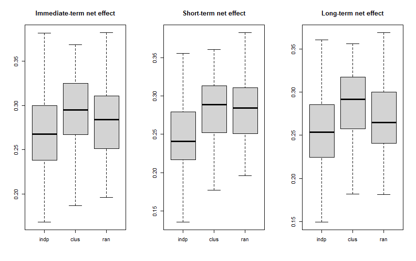
Figure 2: Immediate-term (B $-$ A), short-term (C $-$ A) and long-term net treatment effects (D $-$ A)

Through the construction of the independent set, we prevent spillover of the policy effect and influence among the treated respondents and are thus able to decouple the direct and indirect effects, in the immediate term i.e., in the period immediately following the policy introduction. Hence, by employing the independent set sampling strategy, the estimate of the immediate-term net treatment effect is essentially an estimate of the direct effect of the policy. As shown in Figure 2, we observe a smaller mean immediate-term direct effect and mean short-term net treatment effect for the independent set sampling, as compared to other sampling methods. However, we do note that the mean long-term net treatment effects for the independent set and random samples are similar, implying a convergence in the effectiveness of these two sampling strategies over time. The cluster sampling strategy generally has a larger difference, perhaps due to stronger within-sample signaling which limits its ability to spread the policy effects throughout the network as efficiently as the other effects. We present several statistics, such as the mean and the interquartile range (IQR) of the treatment effects across these three strategies in Appendix F. We ran a Mann-Whitney-Wilcoxon test to compare these proportion differences for the pairwise sampling strategies. We include these $p$-values in Appendix F. Our results show that neither of the net effects differs significantly between random and cluster sampling ($p>0.1$), but that all net effects differ significantly between independent and cluster sampling ($p<0.05$). Interestingly, however, the short-term net effect between the independent set and random sampling is significant ($p<0.01$), whereas the other two effects are not significant ($p>0.1$). Despite the independent sample and random sample techniques not being significantly different in their immediate-term and long-term net effects, the independent set sample may still be a good alternative to the cluster sampling approach for estimating direct as well as net treatment effects of a policy, at least in the immediate and short term, due to its sample selection strategy.

In summary, using the adapted version of the co-evolution model presented in this paper, policymakers are able to estimate the direct and net treatment effects resulting from a policy, as well as the underlying network effects stemming from policy-linked homophily. We contend that policymakers need to consider the distinct homophilous effects generated by the different sampling methods as they affect policy outcomes by shaping the spread of information and behaviors through social networks, and this can result in the propagation of certain behaviors and beliefs through the formation of new homophilous connections. By understanding these dynamics, policymakers can design policies using appropriate sampling methods that can leverage the power of the underlying network effects to achieve the intended policy outcomes more efficiently. As different sampling strategies are shown to give rise to varying levels of net treatment effects, this indicates that having potential connections between respondents in the treatment group affects the estimation of the policy effectiveness. Policymakers need to be wary of the presence of these underlying network effects that can confound policy evaluation results. Furthermore, we show that respondents sampled using our proposed technique will likely be more differentiated in their behavioral characteristics since they were unconnected to each other, prior to the selection. This might also help to promote greater diversity in the selected sample.

5 Discussion

5.1 Summary of key findings

In the current study, we develop a novel sampling strategy based on independent set selection and investigate its efficacy in a policy implementation and evaluation exercise. We contend that this sampling technique is a good alternative to the popularly used cluster sampling technique, especially in contexts where policymakers might prefer a more diverse sample of unconnected respondents. To test the relative effectiveness of this sampling technique against comparable alternatives, we augment a SAOM with independent set sampling, random sampling, or cluster sampling techniques, to analyze the co-evolution of the policy-linked behavior and social network structure. Our simulation results demonstrate the role of the sampling design in influencing the impact of the policy on the population through the changes in both the respondents’ network structure as well as their behavior.

In our study, we adopt an actor-oriented and co-evolution-based MCMC modeling approach from Snijders et al. (2007) to estimate the co-evolution of users’ focal behavior and their social network [78]. To isolate and estimate the direct and net treatment effects of the policy, we employ a second-order difference approach, where we track the proportion of individuals having the focal behavior in the treatment against the non-treatment group over specific stages in time. Since different sampling methods generate dissimilar network structures in the treatment and non-treatment groups, these groups would experience varying levels of network interference. Consequently, our results show a distinction in the net policy effects across the three sampling methods, notably a lower direct and short-term net treatment effect estimate for our proposed independent set sampling method. This reduction can be attributed to the construction of the independent set which prevents spillover of the treatment within the treatment group, in the immediate term.

The estimation results also offer interesting insights into how the network evolves and, in turn, influences the respondents’ focal behavior. Specifically, we find that the respondents are more likely to form ties with others who have similar focal behavior, especially with those in the same treatment group (i.e., co-exposed to the policy). Our results also show that independent set sampling leads to a significant positive homophilous effect based on the policy-linked behavior. Since we eliminate any direct contact between the sampled respondents, the detected homophilous effect can be largely attributed to the policy implementation and its subsequent effects. However, interestingly, we do not observe a significant peer influence across the sampling conditions, once we account for homophily. This is consistent with past studies highlighting that influence often tends to be over-estimated in the absence of homophily [2].

Understanding the role of sampling strategies in policy design has clear practical implications for policymakers with regard to both implementation cost, as well as the varying effects on the population. Based on our design framework and comparative analyses presented in this paper, policymakers can optimize the policy implementation based on available resources, while still retaining a large diversity of respondents and amplifying the impact through homophilous network formation and spreading.

5.2 Future extensions

In this study, we present the design of a simple and specific (maximal) independent set sampling strategy. However, as discussed earlier, there can be multiple independent sets for a given social network. To analyze how these different independent sets can affect policy cost-effectiveness, we can adapt the independent set selection strategy in various ways. For instance, we can seek to maximize certain specified centrality measures of the independent set sample. As an example, we can maximize the degree sum of all the vertices in the independent set, whose size can be chosen with reference to the bounds of $\alpha(G)$. Moreover, policymakers may also have certain size or budget constraints to work with. We can then find this independent set by solving the following integer program, with $A_{G}$ as the adjacency matrix of the graph $G=(V,E)$, $x$ as the vertex incidence vector, $d$ as the degree vector and $c$ as the cost vector of selecting a particular actor into the treatment set.

$$\max\; d^{T}x$$ (21)

s.t. $$\mathbf{1}^{T}x\leq m$$

$$c^{T}x\leq b$$

$$x^{T}A_{G}x=0$$

$$x\in\{0,1\}^{|V(G)|}$$

where $m$ is the size of the independent set, $b$ is the budget, $|V(G)|$ is the number of vertices in the network and $\mathbf{1}$ is the all-one vector. If we require an independent set of a size less than the lower bound of $\alpha(G)$, then there will be a feasible solution to this integer programming problem and we can find such an independent set $I$ with the largest degree sum, where $I$ contains vertex $i$ if $x_{i}=1$. We can change the maximization objective function in the above integer program to incorporate other centrality measures such as closeness, betweenness, page rank, etc.

We also note that it is difficult to practically obtain complete network data, which increases the risk of having unobserved or missing nodes and edges. It is therefore imperative to study the robustness and sensitivity of our proposed models to data incompleteness. One possible way to test this is by relaxing the design of an independent set and allowing a small number of edges to exist within the independent set sample. We can then adjust the above integer program as follows,

$$\max\; d^{T}x$$ (22)

s.t. $$\mathbf{1}^{T}x\leq m$$

$$c^{T}x\leq b$$

$$x^{T}A_{G}x\leq\epsilon$$

$$x\in\{0,1\}^{|V(G)|}$$

where $\epsilon$ is the tolerance of the edges that the policymakers allow. However, we may require careful adjustments to account for the spread of the policy effects within the treatment group.

We can also extend this study by analyzing the sensitivity of our model and estimation results to different graph structures such as Erdos-Renyi or small-world constructions. Through these extensions and robustness tests, we will be able to identify the best independent set to use for a specific type of network structure and one that leads to a more resource-efficient evaluation of the policy.

Another important consideration in policy evaluation studies is the propagation of policy effects in a social network, where we could treat the spread of policy-linked behavior as a contagion process. There are several studies that investigate this effect, notably, Kempe et al. (2003) who look at maximizing the spread of influence in a static network context [45]. In a more realistic setting, Zhuang et al. (2013) examine this problem for a dynamic network [96], while Greenan (2015) combines the existing work on SAOM with a proportional hazard model to investigate the contagion spread in an evolving social network [34]. We can also consider how different seeding strategies affect the spread of the policy effect while incorporating behavioral decisions through a threshold-based model [33]. Furthermore, we can study the sensitivity of the propagation to distinct network structures and behavioral thresholds.

5.3 Limitations

Since this study is among the first to analyze the role of network sampling strategies in policy evaluation, it is important to acknowledge certain limitations and challenges. Firstly, as mentioned earlier, we require access to complete network data to construct an independent set, which might be infeasible in certain policy contexts. We do note that this is a common limitation across several sampling strategies, although certain sampling techniques such as random sampling may be more immune to this. Secondly, in the absence of any prior experimental datasets based on independent set sampling, we resort to a stylized simulation study in this paper to test the relative effectiveness of the sampling strategies. Future empirical studies performed in a real-world experimental context can seek to test the effectiveness of our proposed sampling technique. Thirdly, the need to generate large networks at every stage of the simulation process can be computationally expensive, even for mid-sized networks, and this creates a need for significant computational resources. On a related point, since the SAOM requires probabilistic changes in network and behavior, their estimation can occasionally suffer from convergence issues, thereby requiring additional iterations of model specification and training. Fourthly, though our paper proposes an alternative sampling strategy, we do acknowledge that implementing a policy on any group of people, regardless of the seeding strategy, requires careful execution. In our analysis, we assume that the respondents are largely policy-abiding and do not exhibit non-compliant or anomalous behavior. However, future work can investigate the sensitivity of the proposed model to varying levels of non-compliance. Lastly, all our models rely on a standard Markovian assumption of the data. Although this is a popular assumption in SAOM-based studies, it may be a strict assumption for certain study contexts where there are external shocks affecting either the network formation or the behavior change.

6 Conclusion

Evaluating the impact of social and economic policies is critical to organizations and governments worldwide. The problem of policy evaluation in a networked context has remained under-studied, owing to various methodological limitations with existing work. In this paper, we present a novel empirical strategy that combines an independent set sampling technique with a stochastic actor-oriented modeling (SAOM) approach to disentangle the direct effect of a policy from the net effect, which is often a combination of the direct and network-related effects of the policy. Our results using a simulated policy implementation exercise highlight that our proposed approach leads to distinct estimates of the direct and net effects of the policy. Furthermore, our model allows for the flexible estimation of policy-linked network effects, such as policy-linked homophily, that form a key component of the net effect of the policy. We contend that this is among the first studies to offer a context- and policy-agnostic empirical strategy to estimate policy effects as well as associated policy-linked network effects. Hence, the methods and specifications presented in this paper are likely to be useful for decision-makers in a wide variety of organizational and public policy contexts.

Appendix A Structural Preservation of Maximal Independent Sets

To test the robustness of picking any arbitrary maximal independent set for our simulation study, we provide several statistics, such as mean degree, mean transitivity, and the pairwise Jenson-Shannon Divergence score based on the maximal independent sets generated from over 500 scale-free networks with a scale factor of 2.5.

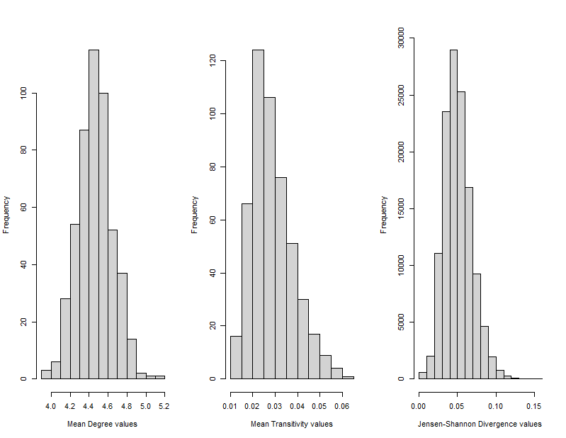
Figure 3: Common network descriptives of the maximal independent sets from 500 networks

From Figure 3, we observe that the mean degree of the independent set samples is 4.466, with a standard deviation of 0.157, and a mean transitivity of 0.028, with a standard deviation of 0.01. To check the similarity of the degree distribution between these samples, we compute the Jenson-Shannon Divergence scores. By computing this score for each pairwise degree distribution, we obtain a mean divergence score of 0.047, with a standard deviation of 0.019.

Appendix B Data Specification

Descriptive summary of the 300 observations used in our study, which is a subset of the data from [93].

Behavior and Covariate Characteristics	Min	1st Quartile	Median	Mean	3rd Quartile	Max
Years of schooling	6	10	12	12.59	15	18
Age (years)	17	28	39	42.18	53	88
Annual income (in USD)	500	12500	20000	19400	30000	30000
Price (cents)	52.8	58.79	61.05	61.10	62.16	70.13

Table 3: Descriptive summary of education level, age, annual income, and prices

Out of the 300 respondents, there are 108 individuals having the focal behavior. As we assign each respondent a gender feature variable with a probability of 60% being male and 40% being female, the realized sample comprises 174 males and 126 females.

Appendix C Stochastic Approximation

In this study, we use a Method of Moments (MoM)-based estimator for the co-evolution model, as described in Subsection 4.2 [9]. The MoM estimator that we use for our network data $A$ and behavioral data $B$, and their corresponding parameter sets $\phi^{[A]}$ and $\phi^{[B]}$ is based on a set of network and behavioral statistics $S_{t}^{[A]}$ and $S_{t}^{[B]}$. The estimator is defined as the parameter value set for which the following conditions are satisfied.

$$\mathbb{E}_{\phi^{[A]}}(S^{[A]})=s^{[A]}(a,b)$$ (23)

$$\mathbb{E}_{\phi^{[B]}}(S^{[B]})=s^{[B]}(a,b)$$ (24)

In other words, the expected values are equivalent to the observed values of the above-mentioned statistics in Subsection 4.2. We note that the conditional expectations from the moment equations (Eqn 23 and 24) cannot be computed explicitly. Hence, we need to employ the stochastic approximation algorithm by [68] to numerically solve for them. The algorithm solves both equations by iteratively generating a parameter sequence $\hat{\phi}$ as follows,

$$\hat{\phi}_{t+1}^{[A]}=\hat{\phi}_{t}^{[A]}-\sigma_{t}D_{0}^{-1}(S_{t}^{[A]}-s^{[A]})$$ (25)

$$\hat{\phi}_{t+1}^{[B]}=\hat{\phi}_{t}^{[B]}-\sigma_{t}D_{0}^{-1}(S_{t}^{[B]}-s^{[B]})$$ (26)

where $S_{t}^{[A]}$ and $S_{t}^{[B]}$ are generated according to the distributions as defined by $\hat{\phi}_{t+1}^{[A]}$ and $\hat{\phi}_{t+1}^{[B]}$ respectively and $D_{0}^{-1}$ is the identity matrix. We need to choose a step size $\sigma_{t}$ such that this sequence converges to zero, for which we can conveniently choose $\sigma_{t}=\frac{a}{b+t}$. We note that this sequence converges to zero for any two integers $a$ and $b$. Snijders [74] shows that the convergence properties of this algorithm hold asymptotically for when $t$ approaches $\infty$ ruppert1988polyak1990yin1991.

Appendix D Descriptive Summary of SAOM Results

Independent set sample

	Time Period
Stage	1	2	3	4
Density	0.020	0.020	0.020	0.020
Average Degree	6.000	6.013	6.013	6.073
Number of Ties	900	902	902	911
Missing Fraction	0	0	0	0

Table 4: Descriptive summary for social network data for independent set sample

	Change in Ties
Period	$0=>0$	$0=>1$	$1=>0$	$1=>1$	Jaccard	Missing
$1=>2$	43948	2	0	900	0.998	0
$2=>3$	43948	0	0	902	1	0
$3=>4$	43939	9	0	902	0.990	0

Table 5: Social network evaluation summary for independent set sample

We note that the Jaccard index is defined as the fraction $\frac{N_{11}}{N_{01}+N_{10}+N_{11}}$, where $N_{ij}$ is the number of the tie variables with value $i$ in one wave, or observation from our generated dataset, and the value $j$ in the next wave.

	Time Period
Stage	1	2	3	4
Number of individuals not having focal behavior	192	192	241	244
Number of individuals having focal behavior	108	108	59	56

Table 6: Descriptive summary for behavioral data for independent set sample

	Number of users
Period	Lose focal behavior	Attain focal behavior	Constant	Missing
$1=>2$	0	0	300	0
$2=>3$	58	9	233	0
$3=>4$	3	0	297	0

Table 7: Behavior evaluation summary for independent set sample

Random sample

	Time Period
Stage	1	2	3	4
Density	0.020	0.020	0.020	0.020
Average Degree	6.000	6.013	6.013	6.033
Number of Ties	900	902	902	905
Missing Fraction	0	0	0	0

Table 8: Descriptive summary for social network data for random sample

	Change in Ties
Period	$0=>0$	$0=>1$	$1=>0$	$1=>1$	Jaccard	Missing
$1=>2$	43948	2	0	900	0.998	0
$2=>3$	43948	0	0	902	1	0
$3=>4$	43945	3	0	902	0.997	0

Table 9: Social network evaluation summary for random sample

	Time Period
Stage	1	2	3	4
Number of individuals not having focal behavior	192	192	237	237
Number of individuals having focal behavior	108	108	63	63

Table 10: Descriptive summary for behavioral data for random sample

	Number of users
Period	Lose focal behavior	Attain focal behavior	Constant	Missing
$1=>2$	0	0	300	0
$2=>3$	52	7	241	0
$3=>4$	0	0	300	0

Table 11: Behavior evaluation summary for random sample

Cluster sample

	Time Period
Stage	1	2	3	4
Density	0.020	0.020	0.020	0.020
Average Degree	6.000	6.013	6.013	6.0060
Number of Ties	900	902	902	909
Missing Fraction	0	0	0	0

Table 12: Descriptive summary for social network data for cluster sample

	Change in Ties
Period	$0=>0$	$0=>1$	$1=>0$	$1=>1$	Jaccard	Missing
$1=>2$	43948	2	0	900	0.996	0
$2=>3$	43946	0	0	902	1	0
$3=>4$	43941	7	0	902	0.992	0

Table 13: Social network evaluation summary for cluster sample

	Time Period
Stage	1	2	3	4
Number of individuals not having focal behavior	192	192	236	238
Number of individuals having focal behavior	108	108	64	62

Table 14: Descriptive summary for behavioral data for cluster sample

	Number of users
Period	Lose focal behavior	Attain focal behavior	Constant	Missing
$1=>2$	0	0	300	0
$2=>3$	49	5	246	0
$3=>4$	2	0	298	0

Table 15: Behavior evaluation summary for cluster sample

Appendix E Descriptive summary of network estimates from 50 SAOM runs

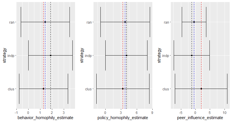
Figure 4: 90% confidence interval of the homophily and peer influence estimates over 50 runs with maximum convergence ratio less than 0.25

Behavior homophily estimates
Strategy	Mean estimates	Root-Mean-Square standard error
Independent	1.8643	1.1322
Cluster	1.2764	1.2580
Random	1.4249	1.2467

Table 16: Descriptive summary of the behavior homophily estimates over 50 runs

Policy homophily estimates
Strategy	Mean estimates	Root-Mean-Square standard error
Independent	4.010	2.4355
Cluster	3.3222	3.0884
Random	3.7698	2.8839

Table 17: Descriptive summary of the policy homophily estimates over 50 runs

Peer influence estimates
Strategy	Mean estimates	Root-Mean-Square standard error
Independent	-1.3326	3.7557
Cluster	1.9467	5.4768
Random	-0.4999	2.5531

Table 18: Descriptive summary of the peer influence estimates over 50 runs

Appendix F Statistics of Net and Direct Effects

Statistics of the second order difference
Mean Direct Effect	Independent	0.267
	Random	0.283
	Cluster	0.292
IQR of Mean Direct Effect	Independent	0.062
	Random	0.060
	Cluster	0.058
Mean Short term Net Effect	Independent	0.247
	Random	0.283
	Cluster	0.280
IQR of Mean Short term Net Effect	Independent	0.063
	Random	0.60
	Cluster	0.061
Mean Long term Net Effect	Independent	0.253
	Random	0.271
	Cluster	0.283
IQR of Mean Long term Net Effect	Independent	0.061
	Random	0.059
	Cluster	0.060

Table 19: Statistics of direct and net effects in Fig. 2 for all 3 sampling strategies

$p$-value for pairwise strategies
Direct effect: Independent vs. Random	0.144
Direct effect: Cluster vs. Random	0.309
Direct effect: Independent vs. Cluster	0.024
Short-term net effect: Independent vs. Random	0.002
Short-term net effect: Cluster vs. Random	0.935
immediate-term net effect: Independent vs. Cluster	0.005
Long-term net effect: Independent vs. Random	0.140
Long-term net effect: Cluster vs. Random	0.182
Long-term net effect: Independent vs. Cluster	0.012

Table 20: $p$-values from Mann-Whitney-Wilcoxon tests for pairwise sampling strategies

References

- [1] Jimi Adams and David Schaefer “How Initial Prevalence Moderates Network-based Smoking Change: Estimating Contextual Effects with Stochastic Actor-based Models” In Journal of Health and Social Behavior 57, 2016, pp. 22–38
- [2] Sinan Aral, Lev Muchnik and Arun Sundararajan “Distinguishing influence-based contagion from homophily-driven diffusion in dynamic networks” In Proceedings of the National Academy of Sciences 106.51 National Acad Sciences, 2009, pp. 21544–21549
- [3] Pierre-Alexandre Balland, José Antonio Belso-Martínez and Andrea Morrison “The Dynamics of Technical and Business Knowledge Networks in Industrial Clusters: Embeddedness, Status, or Proximity?” In Economic Geography 92.1, 2016, pp. 35–60
- [4] Guillaume Basse and Edoardo Airoldi “Limitations of Design-based Causal Inference and A/B Testing under Arbitrary and Network Interference” In Sociological Methodology 48, 2017, pp. 136–151
- [5] Per Block, Christoph Stadtfeld and Tom Snijders “Forms of Dependence: Comparing SAOMs and ERGMs From Basic Principles” In Sociological Methods & Research 48.1 Sage Publications Sage CA: Los Angeles, CA, 2016, pp. 202–239
- [6] Vincent Blondel, Jean-Loup Guillaume, Renaud Lambiotte and Etienne Lefebvre “Fast Unfolding of Communities in Large Networks” In Journal of Statistical Mechanics Theory and Experiment 2008, 2008
- [7] Lawrence E Blume, William A Brock, Steven N Durlauf and Yannis M Ioannides “Identification of social interactions” In Handbook of social economics 1 Elsevier, 2011, pp. 853–964
- [8] Susana Borrás and Mart Laatsit “Towards system oriented innovation policy evaluation? Evidence from EU28 member states” In Research Policy 48.1 Elsevier, 2019, pp. 312–321
- [9] K.O. Bowman and L.. Shenton “Method of Moments” In Encyclopedia of Statistical Sciences 5 New York: Wiley, 1985, pp. 467–473
- [10] Yann Bramoullé, Habiba Djebbari and Bernard Fortin “Identification of peer effects through social networks” In Journal of Econometrics 150.1, 2009, pp. 41–55
- [11] William A Brock and Steven N Durlauf “Interactions-based models” In Handbook of econometrics 5 Elsevier, 2001, pp. 3297–3380
- [12] Jasperina Brouwer et al. “The development of peer networks and academic performance in learning communities in higher education” In Learning and Instruction 80, 2022, pp. 101603
- [13] Yair Caro “New results on the independence number”, 1979
- [14] Julian TszKin Chan “Snowball Sampling and Sample Selection in a Social Network” 42, Advances in Econometrics, 2020, pp. 61–80
- [15] Yong Hyo Cho “A Multiple Regression Model for the Measurement of the Public Policy Impact on Big City Crime” In Policy Sciences 3.4, 1972, pp. 435–455
- [16] J.R. Cole “Fair Science: Women in the Scientific Community”, 1979
- [17] A Coly and G Parry “Evaluating complex health interventions: a guide to rigorous research designs” In Academy Health, 2017
- [18] Thomas D Cook, Donald Thomas Campbell and William Shadish “Experimental and quasi-experimental designs for generalized causal inference” Houghton Mifflin Boston, MA, 2002
- [19] Laurent Davezies, Xavier D’Haultfoeuille and Denis Fougère “Identification of peer effects using group size variation” In The Econometrics Journal 12.3, 2009, pp. 397–413
- [20] Giacomo De Giorgi, Michele Pellizzari and Silvia Redaelli “Identification of Social Interactions through Partially Overlapping Peer Groups” In American Economic Journal: Applied Economics 2.2, 2010, pp. 241–75
- [21] Bruce A. Desmarais and Skyler J. Cranmer “Statistical Inference for Valued-Edge Networks: The Generalized Exponential Random Graph Model” In PLOS ONE 7.1 Public Library of Science, 2012, pp. 1–12
- [22] Dean Eckles, Brian Karrer and Johan Ugander “Design and Analysis of Experiments in Networks: Reducing Bias from Interference” In Journal of Causal Inference 5, 2016
- [23] John H. Enns “The Response of State Highway Expenditures and Revenues to Federal Grants-in-Aid.” RAND Corporation, 1974
- [24] Dennis Epple and Richard E Romano “Peer effects in education: A survey of the theory and evidence” In Handbook of social economics 1 Elsevier, 2011, pp. 1053–1163
- [25] Santo Fortunato “Community detection in graphs” In Physics Reports 486.3, 2010, pp. 75–174
- [26] Paul J Gertler et al. “Impact evaluation in practice” World Bank Publications, 2016
- [27] Saeid Ghafouri and Seyed Hossein Khasteh “A survey on exponential random graph models: An application perspective” In PeerJ Computer Science 6, 2020, pp. e269
- [28] Elisa Giuliani “Network dynamics in regional clusters: Evidence from Chile” In Research Policy 42.8 Elsevier, 2013, pp. 1406–1419
- [29] Leo A. Goodman “Snowball Sampling” In The Annals of Mathematical Statistics 32.1 Institute of Mathematical Statistics, 1961, pp. 148–170
- [30] Holger Graf and Tom Broekel “A shot in the dark? Policy influence on cluster networks” In Research Policy 49.3 Elsevier, 2020, pp. 103920
- [31] Bryan S. Graham “Identifying Social Interactions through Conditional Variance Restrictions” In Econometrica 76.3 [Wiley, Econometric Society], 2008, pp. 643–660
- [32] Bryan S. Graham and Jinyong Hahn “Identification and estimation of the linear-in-means model of social interactions” In Economics Letters 88.1, 2005, pp. 1–6
- [33] Mark Granovetter “Threshold Models of Collective Behavior” In American Journal of Sociology 83.6, 1978, pp. 1420–1443
- [34] Charlotte C Greenan “Diffusion of innovations in dynamic networks” In Journal of the Royal Statistical Society Series A: Statistics in Society 178.1 Oxford University Press, 2015, pp. 147–166
- [35] Magnús Halldórsson and Jaikumar Radhakrishnan “Greed is Good: Approximating Independent Sets in Sparse and Bounded-Degree Graphs.” In Algorithmica 18, 1997, pp. 145–163
- [36] Steve Hanneke, Wenjie Fu and Eric P. Xing “Discrete temporal models of social networks” In Electronic Journal of Statistics 4 Institute of Mathematical StatisticsBernoulli Society, 2010, pp. 585–605
- [37] Eduardo Hariton and Joseph Locascio “Randomised controlled trials - the gold standard for effectiveness research: Study design: randomised controlled trials” In BJOG: An International Journal of Obstetrics & Gynaecology 125.13, 2018, pp. 1716
- [38] Guy Harling, Rui Wang, Jukka-Pekka Onnela and Victor De Gruttola “Leveraging contact network structure in the design of cluster randomized trials” In Clinical Trials 14.1, 2017, pp. 37–47
- [39] Douglas D Heckathorn and Christopher J Cameron “Network sampling: From snowball and multiplicity to respondent-driven sampling” In Annual review of sociology 43 Annual Reviews, 2017, pp. 101–119
- [40] Pili Hu and Wing Lau “A Survey and Taxonomy of Graph Sampling” In arXiv preprint arXiv:1308.5865, 2013
- [41] Robert Huggins “Inter-firm network policies and firm performance: evaluating the impact of initiatives in the United Kingdom” In Research Policy 30.3 Elsevier, 2001, pp. 443–458
- [42] Koen Jochmans “Peer effects and endogenous social interactions” In Journal of Econometrics Elsevier, 2022
- [43] Ida Johnsson and Hyungsik Roger Moon “Estimation of peer effects in endogenous social networks: Control function approach” In The Review of Economics and Statistics 103.2 MIT Press, 2021, pp. 328–345
- [44] Vishesh Karwa and Edoardo Airoldi “A systematic investigation of classical causal inference strategies under mis-specification due to network interference” In arXiv preprint arXiv:1810.08259, 2018
- [45] David Kempe, Jon Kleinberg and Éva Tardos “Maximizing the Spread of Influence through a Social Network” In Proceedings of the Ninth ACM SIGKDD International Conference on Knowledge Discovery and Data Mining Association for Computing Machinery, 2003, pp. 137–146
- [46] Paula Kivimaa and Karoline S Rogge “Interplay of policy experimentation and institutional change in sustainability transitions: The case of mobility as a service in Finland” In Research Policy 51.1 Elsevier, 2022, pp. 104412
- [47] Brendan Kline and Elie Tamer “Some Interpretation of the Linear-In-Means Model of Social Interactions”, 2014
- [48] Gueorgi Kossinets and Duncan J Watts “Origins of homophily in an evolving social network” In American journal of sociology 115.2 The University of Chicago Press, 2009, pp. 405–450
- [49] Lungfei Lee “Identification and estimation of econometric models with group interactions, contextual factors and fixed effects” In Journal of Econometrics 140.2, 2007, pp. 333–374
- [50] Youngmi Lee and In Won Lee “A Longitudinal Network Analysis of Intergovernmental Collaboration for Local Economic Development” In Urban Affairs Review 58.1, 2022, pp. 229–257
- [51] Antony S St Leger and P.. Sweetnam “Statistical problems in studying the relative specificities of association between environmental agents and different diseases: a solution suggested.” In International journal of epidemiology 8 1, 1979, pp. 73–7
- [52] Xinning Liang and Anita MM Liu “The evolution of government sponsored collaboration network and its impact on innovation: A bibliometric analysis in the Chinese solar PV sector” In Research Policy 47.7 Elsevier, 2018, pp. 1295–1308
- [53] G.S. Maddala “Limited-Dependent and Qualitative Variables in Econometrics”, Econometric Society Monographs Cambridge University Press, 1983
- [54] Charles F. Manski “Identification of Endogenous Social Effects: The Reflection Problem” In The Review of Economic Studies 60.3, 1993, pp. 531–542
- [55] Charles F. Manski “Economic Analysis of Social Interactions” In Journal of Economic Perspectives 14.3, 2000, pp. 115–136
- [56] Miller McPherson, Lynn Smith-Lovin and James M Cook “Birds of a feather: Homophily in social networks” In Annual review of sociology 27.1 Annual Reviews 4139 El Camino Way, PO Box 10139, Palo Alto, CA 94303-0139, USA, 2001, pp. 415–444
- [57] Anna Mergoni and Kristof De Witte “Policy evaluation and efficiency: a systematic literature review” In International Transactions in Operational Research 29.3, 2022, pp. 1337–1359
- [58] El Moussaoui Mohamed, Tarik Agouti, Abdessadek Tikniouine and Mohamed El Adnani “A comprehensive literature review on community detection: Approaches and applications” In Procedia Computer Science 151 Elsevier, 2019, pp. 295–302
- [59] Stuart Nicholls et al. “The ethical challenges raised in the design and conduct of pragmatic trials: An interview study with key stakeholders” In Trials 20, 2019, pp. 1–16
- [60] OECD “Improving Governance with Policy Evaluation”, 2020, pp. 170
- [61] Robert Olsen, Larry Orr, Stephen Bell and Elizabeth Stuart “External Validity in Policy Evaluations That Choose Sites Purposively” In Journal of Policy Analysis and Management 32, 2013, pp. 107–121
- [62] Larry L Orr “2014 Rossi award lecture: Beyond internal validity” In Evaluation review 39.2 SAGE Publications Sage CA: Los Angeles, CA, 2015, pp. 167–178
- [63] Lewis J. Perl, Dean T. Jamison and Roy Radner “Graduation, Graduate School Attendance, and Investments in College Training” In Education as an Industry National Bureau of Economic Research, Inc, 1976, pp. 95–148
- [64] Boris Polyak “New method of stochastic approximation type” In Automation and Remote Control 7, 1991, pp. 937–946
- [65] Alan L. Porter, Terry Connolly, Russell G. Heikes and Choon Y. Park “Misleading Indicators: The Limitations of Multiple Linear Regression in Formulation of Policy Recommendations” In Policy Sciences 13.4 Springer, 1981, pp. 397–418
- [66] Sarah Raifman et al. “Respondent-Driven Sampling: a Sampling Method for Hard-to-Reach Populations and Beyond” In Current Epidemiology Reports 9.1, 2022, pp. 38–47
- [67] Ruth M Ripley et al. “Manual for Siena version 4.0” R package version 1.3.14.1. https://www.cran.r-project.org/web/packages/RSiena/, 2023
- [68] Herbert Robbins and Sutton Monro “A Stochastic Approximation Method” In The Annals of Mathematical Statistics 22.3 Institute of Mathematical Statistics, 1951, pp. 400–407
- [69] Garry Robins et al. “Recent developments in exponential random graph (p*) models for social networks” In Social Networks 29, 2007, pp. 192–215
- [70] David Ruppert “Efficient Estimations from a Slowly Convergent Robbins-Monro Process”, 1988
- [71] Martin Saveski et al. “Detecting network effects: Randomizing over randomized experiments” In Proceedings of the 23rd ACM SIGKDD international conference on knowledge discovery and data mining, 2017, pp. 1027–1035
- [72] Tassilo Schwarz “Randomized Controlled Trials Under Influence: Covariate Factors and Graph-Based Network Interference” In arXiv preprint arXiv:2111.14263, 2021
- [73] Cosma Shalizi and Andrew Thomas “Homophily and Contagion Are Generically Confounded in Observational Social Network Studies” In Sociological methods & research 40, 2011, pp. 211–239
- [74] Tom Snijders “The statistical evaluation of social network dynamics” In Sociological methodology 31.1 Wiley Online Library, 2001, pp. 361–395
- [75] Tom Snijders “Models for longitudinal network data” In Models and methods in social network analysis 1, 2005, pp. 215–247
- [76] Tom Snijders “Statistical methods for network dynamics” In Proceedings of the XLIII Scientific Meeting, 2006, pp. 281–296
- [77] Tom Snijders “Siena: Statistical Modeling of Longitudinal Network Data” In Encyclopedia of Social Network Analysis and Mining Springer New York, 2017, pp. 1–9
- [78] Tom Snijders, Christian Steglich and Michael Schweinberger “Modeling the co-evolution of networks and behavior” In Longitudinal Models in the Behavioral and Related Sciences, 2007, pp. 41–71
- [79] Tom A.B. Snijders, Gerhard G. van de Bunt and Christian E.G. Steglich “Introduction to stochastic actor-based models for network dynamics” Dynamics of Social Networks In Social Networks 32.1, 2010, pp. 44–60
- [80] Patrick C. Staples, Elizabeth L. Ogburn and Jukka-Pekka Onnela “Incorporating Contact Network Structure in Cluster Randomized Trials” In Scientific Reports 5.1, 2015, pp. 17581
- [81] Christian Steglich, Tom Snijders and Michael Pearson “Dynamic Networks And Behavior: Separating Selection From Influence” In Sociological Methodology 40, 2010, pp. 329–393
- [82] S.K. Thompson and G.A.F. Seber “Adaptive Sampling”, Wiley Series in Probability and Statistics Wiley, 1996
- [83] Johan Ugander, Brian Karrer, Lars Backstrom and Jon Kleinberg “Graph cluster randomization: Network exposure to multiple universes” In Proceedings of the 19th ACM SIGKDD international conference on Knowledge discovery and data mining, 2013, pp. 329–337
- [84] Johan Ugander and Hao Yin “Randomized graph cluster randomization” In Journal of Causal Inference 11.1 De Gruyter, 2023, pp. 20220014
- [85] Arnaud Vaganay “Cluster Sampling Bias in Government-Sponsored Evaluations: A Correlational Study of Employment and Welfare Pilots in England” In PLOS ONE 11.8 Public Library of Science, 2016, pp. 1–21
- [86] Tyler J. VanderWeele and Weihua An “Social Networks and Causal Inference” In Handbooks of Sociology and Social Research Springer Netherlands, 2013, pp. 353–374
- [87] Davide Viviano “Policy design in experiments with unknown interference” In arXiv preprint arXiv:2011.08174, 2020
- [88] Zheng Wang “The linking effect: causal identification and estimation of the effect of peer relationship” In 4th EUI Alumni Conference in Economics, 2022
- [89] Stan Wasserman and Philippa Pattison “Logit Models and Logistic Regressions for Social Networks: I. An Introduction to Markov Graphs and p*” In Psychometrika 61, 1996, pp. 401–425
- [90] VK Wei “A lower bound on the stability number of a simple graph”, 1981
- [91] D.B. West “Introduction to Graph Theory” Prentice Hall, 1996
- [92] Howard White and David A Raitzer “Impact evaluation of development interventions: A practical guide” Asian Development Bank, 2017
- [93] J.M. Wooldridge “Introductory Econometrics: A Modern Approach” South-Western Cengage Learning, 2015
- [94] G. Yin “On extensions of Polyak’s averaging approach to stochastic approximation” In Stochastics and Stochastic Reports 36.3-4, 1991, pp. 245–264
- [95] Yang Zhou, Hong Cheng and Jeffrey Yu “Graph Clustering Based on Structural/Attribute Similarities.” In Proceedings of the VLDB Endowment 2, 2009, pp. 718–729
- [96] Honglei Zhuang et al. “Influence maximization in dynamic social networks” In 2013 IEEE 13th International Conference on Data Mining, 2013, pp. 1313–1318 IEEE