TNPAR: Topological Neural Poisson Auto-Regressive Model for Learning Granger Causal Structure from Event Sequences

Abstract

Learning Granger causality from event sequences is a challenging but essential task across various applications. Most existing methods rely on the assumption that event sequences are independent and identically distributed (i.i.d.). However, this i.i.d. assumption is often violated due to the inherent dependencies among the event sequences. Fortunately, in practice, we find these dependencies can be modeled by a topological network, suggesting a potential solution to the non-i.i.d. problem by introducing the prior topological network into Granger causal discovery. This observation prompts us to tackle two ensuing challenges: 1) how to model the event sequences while incorporating both the prior topological network and the latent Granger causal structure, and 2) how to learn the Granger causal structure. To this end, we devise a two-stage unified topological neural Poisson auto-regressive model. During the generation stage, we employ a variant of the neural Poisson process to model the event sequences, considering influences from both the topological network and the Granger causal structure. In the inference stage, we formulate an amortized inference algorithm to infer the latent Granger causal structure. We encapsulate these two stages within a unified likelihood function, providing an end-to-end framework for this task.

1 Introduction

Causal discovery from multi-type event sequences plays a pivotal role in a multitude of applications. In the realm of intelligent operation and maintenance, for instance, identifying the causal structure behind alarm data can expedite the pinpointing of critical fault events and the location of root causes Vuković and Thalmann (2022). In social analysis, understanding the causal structure behind users’ behavior sequences can inform the development of effective advertising and marketing strategies Chen et al. (2020); Wu et al. (2022).

A range of methods has been proposed for the causal discovery of multi-type event sequences. They fall into two main categories: 1) constraint-based methods, which utilize independence-based tests or measures to ascertain the causal structure between event types, and 2) point process-based methods, which employ point processes to model the generation process of event sequences. While the former, including methods such as PCMCI (PC with Momentary Conditional Independence test) Runge (2020) and transfer entropy-based method Chen et al. (2020); Mijatovic et al. (2021), is founded on strict assumptions of the causal mechanism assumptions, the latter, like Hawkes process-based methods Xu et al. (2016); Zhou et al. (2013); Eichler et al. (2017) and neural point process models Shchur et al. (2021); Chen et al. (2021), is grounded in the concept of Granger causality Granger (1969). Given the weaker assumption of Granger causality, identifying the Granger causal structure just by assessing if a series is predictive of another, point process-based methods often find preference in real-world applications Shojaie and Fox (2022) and are therefore the focal point of this work.

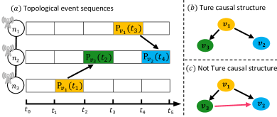
Figure 1: An illustrative example of the topological event sequences generated by a mobile network in an operation and maintenance scenario. In this context, $\{n_{1},n_{2},n_{3}\}$ represent the network elements, and $\{v_{1},v_{2},v_{3}\}$ denote the event types of the alarms. The term $\mathrm{P}_{v_{1}}(t_{1})$ stands for the distribution of $v_{1}$ alarm at $t_{1}$ timestamp, and so on. Black arrows highlight the correct causal edges, whereas the red arrow represents an incorrect edge. (a) Generation process of topological event sequences. The event distribution varies with time and is influenced by both a topological network (connected by the solid lines) and a Granger causal structure (depicted in part (b)). (b) Ground truth of the Granger causal structure. (c) Granger causal structure learned under i.i.d. assumption.

However, these existing point process-based methods are significantly dependent on the i.i.d assumption (that the event sequences are independent and identically distributed) to model the generation process of event sequences. In reality, this assumption often falls short due to the complex dependencies that permeate sequences. Consequently, the performance of these methods often leaves much to be desired in real-world applications. For instance, non-i.i.d. alarm event sequences in an operation and maintenance scenario, as illustrated in Fig. 1, highlight this issue. These event sequences are produced by network elements interconnected by a topological network, indicating the event sequences of different elements are dependent on each other, thereby violating the i.i.d. assumption. In this illustrated scenario, the event type $v_{2}$ in $n_{2}$ is only caused by the event types in topologically connected elements (specifically, $v_{1}$ in $n_{2}$). Existing methods would incorrectly identify the edge $v_{3}\rightarrow v_{2}$ because they erroneously treat event sequences on different nodes as independent. By incorporating the topological network, we can correctly learn that $v_{2}$ is actually caused by $v_{1}$ and discern the true causal structure. Therefore, it is vital to exploit the topological network to model the dependencies among non-i.i.d. event sequences and accurately recover the causal structure from them.

This gives rise to two ensuing challenges: 1) how to explicitly model the generation process of topological event sequences, incorporating both the prior topological network and the latent causal structure, and 2) how to learn the latent Granger causal structure from topological event sequences. To tackle these challenges, Cai et al. Cai et al. (2022) propose the topological Hawkes process (THP), which extends the time-domain convolution property of the Hawkes process to the time-graph domain. Nevertheless, THP’s applicability in real-world scenarios remains limited due to the complex generation process and distribution of real events, which are often too intricate to be accurately represented by the Hawkes process. Consequently, Hawkes process-based methods often suffer from oversimplified generation functions and specified distributions. Hence, it is crucial to devise a distribution-free generation model that can incorporate both the topological event sequences and the latent Granger causal structure.

In response to these challenges, we develop a unified Topological Neural Poisson Auto-Regressive (TNPAR) model, comprising a generation process and an inference process. In the generation process, we introduce a variant of the Poisson Auto-Regressive model to depict the generation process of topological event sequences. By extending the Auto-Regressive model with Poisson Process and incorporating both the topological network and the Granger causal structure, TNPAR effectively overcomes the non-i.i.d. problem. By representing the distribution using a series of Poisson processes with varying parameters, TNPAR displays enhanced flexibility compared to existing methods that employ a single fixed distribution for the entire sequence. For the inference process, inspired by the generative model that treats the causal structure as a latent variable Li et al. (2021), we design an amortized inference algorithm Zhang et al. (2018); Gershman and Goodman (2014) to learn the Granger causal structure. By integrating these generation and inference procedures, we establish a unified likelihood function for our TNPAR model, which can be optimized within an end-to-end paradigm.

In summary, our main contributions are as follows:

1. We develop a topological neural Poisson auto-regressive method that accurately learns causal structure from topological event sequences.

2. Our method incorporates the prior topological network into the generation process, offering a solution to the non-i.i.d. challenge in causal discovery.

3. By treating the causal structure as a latent variable, we devise an amortized inference method to identify the causal structure among the event types.

2 Related work

This section presents the related work on Granger causal discovery from event sequences. We have also provided a comparison of our work with related methods in Appendix A.

2.1 Temporal Point Process

Temporal point processes are stochastic processes utilized to model event sequences. Current work based on temporal point processes can be bifurcated into two main categories: statistical point processes and neural point processes. On the one hand, statistical point processes rely on parametric methods whose functions often possess specific physical interpretations. Notable examples of statistical point processes encompass the Poisson process Cox (1955), Hawkes process Hawkes (1971), reactive point process Ertekin et al. (2015), self-correcting process Isham and Westcott (1979), and Graphical Event Models Gunawardana and Meek (2016); Bhattacharjya et al. (2018), among others. Conversely, neural point processes Shchur et al. (2021); Chen et al. (2021) exploit the potent learning capabilities of neural networks to model sequences, often outperforming statistical point process methods in prediction performance. These methods are typically predicated on recurrent neural networks and their variants.

2.2 Granger Causality for Event Sequences

Current point process-based Granger causal discovery algorithms for event sequences can be classified into two primary types: the Hawkes process-based methods and the neural point process-based methods. The fundamental assumption of the Hawkes process is that past events stimulate the occurrence of related events in the future. Typical Hawkes process-based methods Zhou et al. (2013); Xu et al. (2016) are focused on designing appropriate kernel functions and regularization techniques. Recently, the THP algorithm Cai et al. (2022) extends the Hawkes process to address the non-i.i.d. issue by employing a topological-temporal convolutional kernel function to model the interdependencies among event sequences. In contrast, neural point process-based methods Xiao et al. (2019); Zhang et al. (2020) do not depend on specific assumptions of generation functions like the Hawkes process. Instead, they employ neural networks to model event sequences, leveraging the expressive power of these networks.

In another vein, some studies model event sequences using time series-based models, such as auto-regressive and constraint-based methods. For instance, Brillinger Brillinger (1994) transforms event sequences into time series, which enables the analysis of event sequences using auto-regressive models. The Granger Causality alignment (GCA) model Li et al. (2021) combines the auto-regressive model with the generation model to learn the Granger causality. PCMCI Runge (2020) extends the PC algorithm Spirtes et al. (2000) to time series data. However, none of these approaches considers the non-i.i.d. event sequences within a topological network.

3 Granger Causal Discovery using Neural Poisson Auto-Regressive

3.1 Problem Definition

Let an undirected graph $\mathcal{G}_{N}(\mathbf{N},\mathbf{E}_{N})$ represent the topological network among nodes $\mathbf{N}$, and a directed graph $\mathcal{G}_{V}(\mathbf{V},\mathbf{E}_{V})$ represent the causal graph among event types $\mathbf{V}$. In this context, $\mathbf{E}_{N}$ signifies the physically connected edges between nodes, and $\mathbf{E}_{V}$ denotes the causal edges between event types. A series of topological event sequences of length $m$, symbolized as $\mathbf{X}=\{(v_{i},n_{i},t_{i})|i\in\{1,\ldots,m\}\}$, are generated by a Granger causal structure $\mathcal{G}_{V}(\mathbf{V},\mathbf{E}_{V})$ within a topological network $\mathcal{G}_{N}(\mathbf{N},\mathbf{E}_{N})$. Each item in the series consists of $v_{i}\in\mathbf{V}$ representing the event type, $n_{i}\in\mathbf{N}$ representing the topological node, and $t_{i}\in[0,T]$ representing the occurrence timestamp. We can consider the topological event sequences $\mathbf{X}$ as a set of counting processes $\{\mathrm{C}_{v_{i},n_{j}}(t)|v_{i}\in\mathbf{V},n_{j}\in\mathbf{N},t\in[0,T]\}$, where $\mathrm{C}_{v_{i},n_{j}}(t)$ denotes the count of event type $v_{i}$ that has occurred up to $t$ at $n_{j}$. In this work, we divide the continuous interval $[0,T]$ into $T/\Delta$ small intervals, where $\Delta\in\mathbb{R}^{+}$. Within each small interval, we assume that the counting process follows a Poisson process Stoyan et al. (2013).

Based on the above definition, we can extend occurrence numbers of event sequences within the interval $\Delta$, denoted as $\mathbf{O}^{V}=\{O_{t}^{v_{i}}|t\in\{1,\ldots,T/\Delta\},i\in\{1,\ldots,|\mathbf{V}|\}\}$, to occurrence numbers of topological event sequences $\mathbf{O}^{V,N}=\{O_{t}^{v_{i},n_{j}}|t\in\{1,\ldots,T/\Delta\},i\in\{1,\ldots,|\mathbf{V}|\},j\in\{1,\ldots,|\mathbf{N}|\}\}$. Here, $O_{t}^{v_{i},n_{j}}$ represents the number of occurrences of event type $v_{i}$ at node $n_{j}$ within the time interval $(t,t+\Delta]$. The specific value of $\Delta$ can be determined according to the requirements of real-world applications.

As each counting process adheres to a Poisson process in a small interval $\Delta$, the number of occurrences $O^{v_{i},n_{j}}_{t}=\mathrm{C}_{v_{i},n_{j}}(t+\Delta)-\mathrm{C}_{v_{i},n_{j}}(t)$ can be modeled by a Poisson random variable with parameter $\lambda^{v_{i},n_{j}}_{t}$. Thus, the probability of $O^{v_{i},n_{j}}_{t}=o$ is expressed as:

$$\mathrm{P}(O^{v_{i},n_{j}}_{t}\!=\!o)\!=\frac{(\lambda^{v_{i},n_{j}}_{t}\Delta)^{o}}{o!}e^{-\lambda^{v_{i},n_{j}}_{t}\Delta};o=0,1,...$$ (1)

Consequently, we can formulate the problem of causal discovery from topological event sequences as:

Definition 1 (Causal discovery from topological event sequences).

Given the occurrence numbers of topological event sequences, $\mathbf{O}^{V,N}=\{O_{t}^{v_{i},n_{j}}|t\in\{1,\ldots,T/\Delta\},i\in\{1,\ldots,|\mathbf{V}|\},j\in\{1,\ldots,|\mathbf{N}|\}\}$, and the prior topological network $\mathcal{G}_{N}(\mathbf{N},\mathbf{E}_{N})$, the goal of causal discovery from topological event sequences is to infer the Granger causal structure $\mathcal{G}_{V}(\mathbf{V},\mathbf{E}_{V})$ among the event types.

In the following, we model the generation process of these topological event sequences by extending an auto-regressive model with the Poisson process to accommodate the non-i.i.d. nature of the data. Furthermore, we devise an amortized inference method to solve the above problem of inferring the latent Granger causal structure.

3.2 Generation Process of the Event Sequences via Topological Neural Poisson Auto-Regressive Model

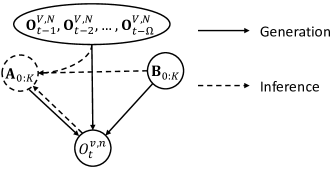
Figure 2: An illustration of the generation and inference processes for TNPAR. In this figure, $\mathbf{A}_{0:K}$ represents the causal matrices of $\mathcal{G}_{V}$, and $\mathbf{B}_{0:K}$ represents the topological matrices of $\mathcal{G}_{N}$. The solid lines signify the generation process for the data $O_{t}^{v,n}$, while the dashed lines denote the inference process for the causal matrices $\mathbf{A}_{0:K}$.

The generation process of TNPAR is depicted using solid lines in Fig. 2. In this process, the current occurrence number of event type $v_{i}$ at node $n_{j}$ (denoted as $O_{t}^{v_{i},n_{j}}$) is determined by a combination of historical data $\{\mathbf{O}^{V}_{t-1},\mathbf{O}^{V}_{t-2},\dots,\mathbf{O}^{V}_{t-\Omega}\}$, the causal matrices $\mathbf{A}_{0:K}$, and the topological matrices $\mathbf{B}_{0:K}$. Here, $\mathbf{A}_{0:K}$ represents a set of matrices $\{\mathbf{A}_{0},\mathbf{A}_{1},\dots,\mathbf{A}_{K}\}$, where $\mathbf{A}_{k}$ is a $|\mathbf{V}|\times|\mathbf{V}|$ binary matrix that indicates the Granger causality between event types at a geodesic distance Bouttier et al. (2003) of $k$ within $\mathcal{G}_{N}$. Let $A_{k}^{i,j}$ denote the element in row $i$ and column $j$ of $\mathbf{A}_{k}$. Then, if $A_{k}^{i,j}=0$, it implies that, at a geodesic distance of $k$, event type $v_{i}$ does not have a Granger causality with $v_{j}$. Conversely, if $A_{k}^{i,j}=1$, then, at a geodesic distance of $k$, a Granger causality exists from $v_{i}$ to $v_{j}$. Similarly, $\mathbf{B}_{0:K}$ corresponds to another set of matrices $\{\mathbf{B}_{0},\mathbf{B}_{1},\dots,\mathbf{B}_{K}\}$, each of which $\mathbf{B}_{k}$ is a $|\mathbf{N}|\times|\mathbf{N}|$ binary matrix that indicates the physical connections of nodes at a geodesic distance of $k$. Let $B_{k}^{i,j}$ denote the element in row $i$ and column $j$ of $\mathbf{B}_{k}$. If the geodesic distance between node $n_{i}$ and $n_{j}$ is $k$ in $\mathcal{G}_{N}$, then $B_{k}^{i,j}=1$. Otherwise, $B_{k}^{i,j}$ will be set to $0$.

In this work, we devise a model, combining the neural auto-regressive model and the Poisson process, to describe the above generation process. To initiate, we introduce a traditional neural auto-regressive model with $\Omega$ time lags:

$$O_{t}^{v_{i}}=\mathrm{g}(\mathbf{O}^{V}_{t-1:t-\Omega})+\epsilon_{t}^{v_{i}},$$ (2)

where $\mathbf{O}^{V}_{t-1:t-\Omega}=\{\mathbf{O}^{V}_{t-1},\mathbf{O}^{V}_{t-2},\dots,\mathbf{O}^{V}_{t-\Omega}\}$ represents a set of historical data, $\mathrm{g}(\cdot)$ is a nonlinear function implemented by a neural network that generates data in the $t$-th time interval based on the historical data, and $\epsilon_{t}^{v_{i}}$ denotes the noise term for event type $v_{i}$ in the $t$-th time interval. In order to incorporate the topological relationships of nodes into our model, we extend $\mathbf{O}^{V}_{t-1:t-\Omega}$ to include the topologically connected historical data, using the function $\mathrm{f}^{\mathcal{G}_{N}}_{n_{j}}(\mathbf{O}^{V,N}_{t-1:t-\Omega},\mathbf{B}_{0:K})$. This function applies a filter to set the non-topologically connected records for node $n_{j}$ to $0$ in the total historical data $\mathbf{O}^{V,N}_{t-1:t-\Omega}$, based on the topological matrices $\mathbf{B}_{0:K}$. This step effectively removes the non-topologically connected information of node $n_{j}$ from $\mathbf{O}^{V,N}_{t-1:t-\Omega}$. Building upon this, our auto-regressive model, incorporating topological information, can be expressed as follows:

$$O_{t}^{v_{i},n_{j}}=\mathrm{g}(\mathrm{f}^{\mathcal{G}_{N}}_{n_{j}}(\mathbf{O}^{V,N}_{t-1:t-\Omega},\mathbf{B}_{0:K}))+\epsilon_{t}^{v_{i},n_{j}}.$$ (3)

Furthermore, to incorporate the Granger causal relationships among event types into the above model, we substitute $\mathbf{O}^{V,N}_{t-1:t-\Omega}$ in Eq. (3) with a function $\mathrm{f}^{\mathcal{G}_{V}}_{v_{i}}(\mathbf{O}^{V,N}_{t-1:t-\Omega},\mathbf{A}_{0:K}\!)$. This function acts as a filter to set the records of event types that do not have a Granger causality with event type $v_{i}$ to $0$ in the total historical data $\mathbf{O}^{V,N}_{t-1:t-\Omega}$ based on the causal matrices $\mathbf{A}_{0:K}$. By incorporating both the topological network and the Granger causal structure, we propose the following model for generating topological event sequences:

$$O_{t}^{v_{i},n_{j}}\!\!=\!\mathrm{g}(\mathrm{f}^{\mathcal{G}_{N}}_{n_{j}}\!(\mathrm{f}^{\mathcal{G}_{V}}_{v_{i}}(\mathbf{O}^{V,N}_{t-1:t-\Omega},\mathbf{A}_{0:K}\!),\mathbf{B}_{0:K}))\!+\epsilon_{t}^{v_{i},n_{j}}.$$ (4)

3.3 Inference Process of the Granger Causal Structure via Amortized Inference

The inference process of TNPAR is depicted using dashed lines in Fig. 2. As shown in the diagram, the Granger causal structure $\mathbf{A}_{0:K}$ is inferred based on a combination of the current occurrence number $O_{t}^{v_{i},n_{j}}$, historical occurrence numbers $\mathbf{O}^{V,N}_{t-1:t-\Omega}$ and the topological network $\mathbf{B}_{0:K}$. Recently, amortized inference, as an advanced method of variational inference, has garnered substantial interest from scholars Zhang et al. (2018); Gershman and Goodman (2014). This approach leverages powerful functions such as neural networks to generate variational distributions conditioned on input data, thereby reducing the computational cost compared to traditional variation inference. Consequently, we designate the Granger causal structure as the latent variable of amortized inference to implement the inference process.

To amortize the inference task for distribution of data $\mathrm{P}(\mathbf{O}^{V,N})$, we optimize an inference model $\mathrm{h}_{\gamma}$ to predict the variational posterior distribution of Granger causal structure $\mathrm{q}_{\phi}(\mathbf{A}_{0:K}|O_{t}^{v_{i},n_{j}},\mathbf{O}^{V,N}_{t-1:t-\Omega},\mathbf{B}_{0:K})$. Specifically, given the data $O_{t}^{v_{i},n_{j}}$ and $\mathbf{O}^{V,N}_{t-1:t-\Omega}$, as well as the topological network $\mathbf{B}_{0:K}$, we use a recognition model $\mathrm{q}_{\phi}(\mathbf{A}_{0:K}|O_{t}^{v_{i},n_{j}},\mathbf{O}^{V,N}_{t-1:t-\Omega},\mathbf{B}_{0:K})$ to approximate the true posterior $\mathrm{p}_{\theta}(\mathbf{A}_{0:K}|O_{t}^{v_{i},n_{j}},\mathbf{O}^{V,N}_{t-1:t-\Omega},\mathbf{B}_{0:K})$. Here, $\phi$ and $\theta$ represent the variational and generation parameters, respectively.

To learn the optimal values of parameters $\theta$ and $\phi$, we model each item in the occurrence numbers $\mathbf{O}^{V,N}$ with a Poisson process, as described in Eq. (1). Subsequently, we maximize the ensuing likelihood function for each $O_{t}^{v_{i},n_{j}}$:

$$\log\mathrm{P}(O_{t}^{v_{i},n_{j}}|\mathbf{O}^{V,N}_{t-1:t-\Omega},\mathbf{B}_{0:K})$$ (5)

$$= \mathrm{D}_{KL}(\mathrm{q}^{A}_{\phi}||\mathrm{p}^{A}_{\theta})\!+\!\mathcal{L}(\theta,\phi;O_{t}^{v_{i},n_{j}}|\mathbf{O}^{V,N}_{t-1:t-\Omega},\mathbf{B}_{0:K}),$$

where $\mathrm{q}^{A}_{\phi}=\mathrm{q}_{\phi}(\mathbf{A}_{0:K}|\mathrm{h}_{\gamma}(O_{t}^{v_{i},n_{j}},\mathbf{O}^{V,N}_{t-1:t-\Omega}),\mathbf{B}_{0:K})$, $\mathrm{p}^{A}_{\theta}=\mathrm{p}_{\theta}(\mathbf{A}_{0:K}|O_{t}^{v_{i},n_{j}},\mathbf{O}^{V,N}_{t-1:t-\Omega},\mathbf{B}_{0:K})$. In Eq. (5), the right-hand side’s (RHS) first term represents the Kullback-Leibler (KL) divergence of the approximate posterior from the true posterior, and the RHS’s second term is the variational evidence lower bound (ELBO) on the log-likelihood of $O_{t}^{v_{i},n_{j}}$. By defining $\mathcal{L}_{e}$ as the ELBO $\mathcal{L}(\theta,\phi;O_{t}^{v_{i},n_{j}}|\mathbf{O}^{V,N}_{t-1:t-\Omega},\mathbf{B}_{0:K})$, and considering that the KL divergence is non-negative, we can deduce from the Eq. (5) that:

$$\log\mathrm{P}(O_{t}^{v_{i},n_{j}}|\mathbf{O}^{V,N}_{t-1:t-\Omega},\mathbf{B}_{0:K})\geq\mathcal{L}_{e}$$ (6)

$$= \mathbb{E}_{\mathrm{q}^{A}_{\phi}}[-\log\mathrm{q}^{A}_{\phi}+\log\mathrm{p}_{\theta}(O_{t}^{v_{i},n_{j}},\mathbf{A}_{0:K}|\mathbf{O}^{V,N}_{t-1:t-\Omega},\mathbf{B}_{0:K})].$$

Furthermore, the ELBO can be expressed in the following manner:

$$\mathcal{L}_{e}= \mathbb{E}_{\mathrm{q}^{A}_{\phi}}[\log\mathrm{p}_{\theta}(O_{t}^{v_{i},n_{j}}|\mathbf{A}_{0:K},\mathbf{O}^{V,N}_{t-1:t-\Omega},\mathbf{B}_{0:K})]$$ (7)

$$-\mathrm{D}_{KL}(\mathrm{q}^{A}_{\phi}||\mathrm{p}_{\theta}(\mathbf{A}_{0:K})).$$

Building upon this equation, the goal of the inference task is to optimize $\mathcal{L}_{e}$ with respect to both $\phi$ and $\theta$, thereby obtaining the posterior distribution of latent Granger causal structure given the data and the topological network.

3.4 Theoretical Analysis

In this subsection, we will theoretically analyze the identifiability of the proposed model. To do so, we begin with the definition, according to work in Tank et al. (2018), of the Granger non-causality of multi-type event sequences as,

Definition 2 (Granger non-causality of multi-type event sequences).

Given data $\mathbf{O}^{V}$ during time interval $t\in\{1,\dots,T/\Delta\}$, which is generated according to Eq. (2), we can determine the Granger non-causality of event type $v_{i}$ with respect to event type $v_{j}$ as follows: For all $\mathbf{O}^{v_{1}}_{t-1:t-\Omega},...,\mathbf{O}^{v_{|V|}}_{t-1:t-\Omega}$ and $\mathbf{O}^{v_{i}}_{t-1:t-\Omega}\neq\mathbf{O}^{v_{i}^{{}^{\prime}}}_{t-1:t-\Omega}$, if the following condition holds:

$$\mathrm{g}(\mathbf{O}^{v_{1}}_{t-1:t-\Omega},...,\mathbf{O}^{v_{i}}_{t-1:t-\Omega},...,\mathbf{O}^{v_{|V|}}_{t-1:t-\Omega})$$

$$= \mathrm{g}(\mathbf{O}^{v_{1}}_{t-1:t-\Omega},...,\mathbf{O}^{v_{i}^{{}^{\prime}}}_{t-1:t-\Omega},...,\mathbf{O}^{v_{|V|}}_{t-1:t-\Omega}).$$

That is, $O_{t}^{v_{j}}$ is invariant to $O_{t}^{v_{i}}$ with $\mathrm{g}(\cdot)$.

By extending the above definition to the topological event sequences, we define the notion of Granger non-causality of topological event sequences as follows:

Definition 3 (Granger non-causality of topological event sequences).

Assume that the occurrence numbers of event sequences are generated by Eq. (4). We can determine the Granger non-causality of event type $v_{i}$ with respect to event type $v_{j}$ as follows: For all $\mathbf{O}^{v_{1},n_{1}}_{t-1:t-\Omega},...,\mathbf{O}^{v_{|V|},n_{|N|}}_{t-1:t-\Omega}$ and $\mathbf{O}^{v_{i},n_{k}}_{t-1:t-\Omega}\neq\mathbf{O}^{v_{i}^{{}^{\prime}},n_{k}}_{t-1:t-\Omega},k\in\{1,...,|N|\}$, if the following condition holds in all nodes under topological network $\mathcal{G}_{N}$:

$$\mathrm{g}(\mathbf{O}^{v_{1},n_{1}}_{t-1:t-\Omega},...,\mathbf{O}^{v_{i},n_{1}}_{t-1:t-\Omega},...,\mathbf{O}^{v_{i},n_{|N|}}_{t-1:t-\Omega},...,\mathbf{O}^{v_{|V|},n_{|N|}}_{t-1:t-\Omega})$$

$$= \mathrm{g}(\mathbf{O}^{v_{1},n_{1}}_{t-1:t-\Omega},...,\mathbf{O}^{v_{i}^{{}^{\prime}},n_{1}}_{t-1:t-\Omega},...,\mathbf{O}^{v_{i}^{{}^{\prime}},n_{|N|}}_{t-1:t-\Omega},...,\mathbf{O}^{v_{|V|},n_{|N|}}_{t-1:t-\Omega}).$$

That is, $O_{t}^{v_{j}}$ is invariant to $O_{t}^{v_{i}}$ with $\mathrm{g}(\cdot)$ in all nodes under topological network $\mathcal{G}_{N}$.

Definition 3 implies that if two event types are Granger non-causality among a topological network, then they are Granger non-causality across all nodes. Based on this definition, we can derive a proposition about the identification of the model as follows.

Proposition 1.

Given the Granger causal structure $\mathcal{G}_{V}(\mathbf{V},\mathbf{E}_{V})$, the topological network $\mathcal{G}_{N}(\mathbf{N},\mathbf{E}_{N})$ and the max geodesic distance $K$, along with the assumption that the data generation process adheres to Eq. (4), we deduce that $v_{i}\rightarrow v_{j}\notin\mathbf{E}_{V}$, if and only if $A_{k}^{v_{i},v_{j}}=0$ for every $k\in\{0,...,K\}$.

The comprehensive proof of Proposition 1 can be found in Appendix B. This proposition inspires a methodology for TNPAR to identify Granger causality, which involves evaluating whether the elements of $\mathbf{A}_{0:K}$ are zero.

4 Algorithm and Implementation

4.1 Inference Process of TNPAR

In this subsection, we employ an encoder to implement the above inference process of TNPAR. Here, the present data $O_{t}^{v_{i},n_{j}}$ and the historical data $\mathbf{O}^{V,N}_{t-1:t-\Omega}$ are used jointly as inputs to the encoder, with $\mathbf{B}_{0:K}$ serving as a mask. The output is the variational posterior of the Granger causal structure, represented as $\mathrm{q}_{\phi}(\mathbf{A}_{0:K}|O_{t}^{v_{i},n_{j}},\mathbf{O}^{V,N}_{t-1:t-\Omega},\mathbf{B}_{0:K})$.

To elaborate, as described in Eq. (4), each element within $\mathbf{O}^{V,N}_{t-1:t-\Omega}$ is initially filtered in accordance with both $\mathbf{B}_{0:K}$ and $n_{j}$. The resulting values are then combined with $O_{t}^{v_{i},n_{j}}$ and converted into a vector, where each item denotes the representation of the occurrence number at a geodesic distance of $k$ for the corresponding node. Following this, the encoder applies a multilayer perception (MLP) Hastie et al. (2009); Cybenko (1989) to the input, which facilitates the propagation of input information across multiple layers and nonlinear activation functions. Ultimately, the encoder generates the posterior distribution of Granger causal structure, denoted as $\mathrm{q}_{\phi}(\mathbf{A}_{0:K}|\mathrm{h}_{\gamma}(O_{t}^{v_{i},n_{j}},\mathbf{O}^{V,N}_{t-1:t-\Omega}),\mathbf{B}_{0:K})$.

In a manner similar to variational inference for categorical latent variables, we assume that the posterior distribution of each causal edge in the Granger causal structure follows a Bernoulli distribution. More specifically, the encoder produces a latent vector $\mathbf{Z}\in[0,1]^{|\mathbf{V}|\times|\mathbf{V}|\times K}$, where $z_{i,j,k}$, the $(i\times j\times k)$-th element of $\mathbf{Z}$, represents the Bernoulli distribution parameter for corresponding edge. Consequently, $\mathrm{q}_{\phi}(\mathbf{A}_{0:K}|\mathrm{h}_{\gamma}(O_{t}^{v_{i},n_{j}},\mathbf{O}^{V,N}_{t-1:t-\Omega}),\mathbf{B}_{0:K})$ can be expressed as:

$$\mathrm{q}_{\phi}(\mathbf{A}_{0:K}|\mathrm{h}_{\gamma}(O_{t}^{v_{i},n_{j}},\mathbf{O}^{V,N}_{t-1:t-\Omega}),\mathbf{B}_{0:K})$$ (8)

$$=\prod_{i=1}^{|\mathbf{V}|}\prod_{j=1}^{|\mathbf{V}|}\prod_{k=0}^{K}\mathrm{q}_{\phi}(A_{k}^{v_{i},v_{j}}|z_{i,j,k})$$

$$\textrm{ with }\>\>\>\mathrm{q}_{\phi}(A_{k}^{v_{i},v_{j}}=1|z_{i,j,k})=\sigma_{\beta}(z_{i,j,k}).$$

Here, $\sigma_{\beta}(x)=1/(1+\exp(-\beta x))$ denotes the sigmoid function with an inverse temperature parameter $\beta$.

Furthermore, for backpropagation through the samples of the discrete distribution $\mathrm{q}_{\phi}(\mathbf{A}_{0:K}|\mathrm{h}_{\gamma}(O_{t}^{v_{i},n_{j}},\mathbf{O}^{V,N}_{t-1:t-\Omega}),\mathbf{B}_{0:K})$ while training TNPAR, we employ the Gumbel-Softmax trick Jang et al. (2017) to generate a differentiable sample as:

where each $\varepsilon_{*}$ is an i.i.d. sample drawn from the standard Gumbel distribution, while $\tau$ is the temperature parameter controlling the randomness of $\hat{A}_{k}^{v_{i},v_{j}}$.

4.2 Generation Process of TNPAR

Next, we propose a decoder to implement the generation process of $\mathbf{O}_{t}^{V,N}$. In this part, $\mathbf{O}^{V,N}_{t-1:t-\Omega}$ is filtered according to both the estimated $\hat{\mathbf{A}}_{0:K}$ and the prior topological network $\mathbf{B}_{0:K}$, as specified in Eq. (4). This filtered result is then used as input to the decoder. Notably, for neural network training, we treat $\hat{\mathbf{A}}_{0:K}$ as a weight matrix during training, and as a mask during testing. This can be accomplished using soft/hard Gumbel-Softmax sampling. Similar to the encoder, a Multilayer Perceptron (MLP) is utilized in the decoder.

Aligning with numerous works on counting processes that posit the distribution of occurrence numbers $O_{t}^{v_{i},n_{j}}$ in each time interval as stationary Stoyan et al. (2013); Babu and Feigelson (1996); Othmer et al. (1988), we model each $\mathrm{p}_{\theta}(O_{t}^{v_{i},n_{j}}|\mathbf{O}^{V,N}_{t-1:t-\Omega},\mathbf{A}_{0:K},\mathbf{B}_{0:K})$ using a Poisson process as denoted in Eq. (1). In this context, the conditional distribution of $O_{t}^{v_{i},n_{j}}$ can be formalized as:

$$\mathrm{p}_{\theta}(O_{t}^{v_{i},n_{j}}|\mathbf{O}^{V,N}_{t-1:t-\Omega},\mathbf{A}_{0:K},\mathbf{B}_{0:K})$$ (10)

$$\!=\frac{(\lambda_{t}^{v_{i},n_{j}}\!\Delta)^{O_{t}^{v_{i},n_{j}}}}{O_{t}^{v_{i},n_{j}}!}e^{-\lambda_{t}^{v_{i},n_{j}}\!\Delta},$$

where $\lambda_{t}^{v_{i},n_{j}}$, provided by the output of the decoder, represents the intensity parameter of the Poisson process.

4.3 Optimization of TNPAR

Based on the above analysis, we adopt the variational ELBO of variational inference, defined in Eq. (7), as the objective function to estimate parameters $\phi$ and $\theta$ of TNPAR and infer the posterior of latent Granger causal structure. In this context, the RHS’s first term of Eq. (7) represents the reconstruction loss, while the RHS’s second term signifies the Kullback-Leibler loss.

In numerous real-world applications, there is often no causal loop in the causal structure $\mathcal{G}_{V}$ during the generation process of event sequences. For instance, based on experts’ prior knowledge, the causal structure in the aforementioned operation and maintenance scenario of a mobile network is a DAG (Directed Acyclic Graph). With this in mind, we introduce an acyclic constraint proposed by Yu et al. (2019), denoted as:

$$\mathrm{h}(\mathbf{G})\equiv\mathrm{tr}((\mathbf{I}+\frac{1}{|\mathbf{V}|}\mathbf{G})^{|\mathbf{V}|})-|\mathbf{V}|=0,$$ (11)

where $\mathbf{G}$ is a matrix in which $G_{i,j}=0$ signifies that event type $v_{i}$ has no Granger causality with $v_{j}$. Conversely, $G_{i,j}>0$. The function $\mathrm{tr}(\cdot)$ calculates the trace of an input matrix. A causal structure $\mathbf{G}$ is acyclic if and only if $\mathrm{h}(\mathbf{G})=0$; Otherwise, $\mathrm{h}(\mathbf{G})>0$. In this study, we set $G_{i,j}=\sum_{k=0}^{K}A_{k}^{v_{i},v_{j}}$ and populate the diagonal of $\mathbf{G}$ with $0$, which implies that self-excitation is permitted in an acyclic graph. Subsequently, we design an acyclic regular term $\mathcal{L}_{c}$ as:

$$\mathcal{L}_{c}=\mathbb{E}_{\mathrm{q}_{\phi}}[\mathrm{tr}((\mathbf{I}+\frac{1}{|\mathbf{V}|}\mathbf{G})^{|\mathbf{V}|})-|\mathbf{V}|]=0.$$ (12)

Without loss of generality, the causal structure tends to be sparse in most real-world applications. Thus, we employ a $\ell_{1}$-norm sparsity constraint to control the model’s sparsity as follows:

$$\mathcal{L}_{s}=\mathbb{E}_{\mathrm{q}_{\phi}}[\sum_{i=1}^{|\mathbf{V}|}\sum_{j=1}^{|\mathbf{V}|}\sum_{k=0}^{K}A_{k}^{v_{i},v_{j}}]\leq\kappa,$$ (13)

where $\kappa$ is a small positive constant. Therefore, the training procedure of TNPAR boils down to the following constrained optimization:

$$\max~{}\mathcal{L}_{e}\quad\text{s.t.}~{}\mathcal{L}_{c}=0,~{}\mathcal{L}_{s}\leq\kappa.$$

By leveraging the Lagrangian multiplier method, we define the total loss function $\mathcal{L}_{total}$ of TNPAR as:

$$\mathcal{L}_{total}=-\mathcal{L}_{e}+\lambda_{c}\mathcal{L}_{c}+\lambda_{s}\mathcal{L}_{s},$$ (14)

where both $\lambda_{c}$ and $\lambda_{s}$ denote the regularization hyperparameters.

In summary, our proposed model is trained on the occurrence numbers of event sequences using the following objective:

$$(\phi^{\star},\theta^{\star})=\mathop{\arg\min}\limits_{\phi,\theta}\mathcal{L}_{total}.$$ (15)

For model training, we can adopt Adam Kingma and Ba (2015) stochastic optimization.

5 Experiment

In this section, we conduct experiments, applying the proposed TNPAR method and the various baseline methods to both simulated data and real metropolitan cellular network alarm data. For all methods, we employ five different random seeds and present the results in graphical format, with error bars included. Our evaluation metrics for the experiments include Precision, Recall, F1 score Powers (2011), Structural Hamming Distance (SHD), and Structural Intervention Distance (SID) Peters and Bühlmann (2015). Specifically, Precision refers to the fraction of predicted edges that exist among the true edges. Recall is the fraction of true edges that have been successfully predicted. F1 score is the weighted harmonic mean of both Precision and Recall, and is calculated as $F1=\frac{2\times Precision\times Recall}{Precision+Recall}$. SHD represents the number of edge insertions, deletions, or flips needed to transform a graph into another graph. SID is a measure that quantifies the closeness between two DAGs based on their corresponding causal inference statements.

5.1 Dataset

5.1.1 Simulated Data

The simulated data is generated as follows: a) a Granger causal structure $\mathcal{G}_{V}$ and a topological network $\mathcal{G}_{N}$ are randomly generated; b) root event records are generated via the Poisson process using a base intensity parameter $\mu$ in the Hawkes process. These root event records are spontaneously generated by the system; c) based on the root event records, propagated event records are discretely generated according to both the time interval $\Delta$ and the excitation intensity $\alpha$. Here, $\alpha$ represents the event excitation intensity in the Hawkes process. Given that the event sequences can be quite sparse in real-world data, we offer a time interval parameter $\Delta$ to the generation process, dividing the time domain $[0,T]$ to $[0,T/\Delta]$. In this context, the event records can be summarized within the same timestamp. Note that the $\Delta\geq 0$. If $\Delta=0$, it implies the use of the original event sequences.

All simulated data are generated by varying the parameters of the generation process one at a time while maintaining default parameters. We set these default parameters according to the data generation process used in the PCIC 2021 competition, inclusive of the additional parameter $\Delta$, as follows: $\#\textrm{nodes}=40$, $\#\textrm{event type}=20$, $\#\textrm{sample size}=20000$, $\mu=[0.00003,0.00005]$, $\alpha=[0.02,0.03]$, $\Delta=2$.

5.1.2 Metropolitan Cellular Network Alarm Data

The Metropolitan Cellular Network alarm event data, which was collected in a business scenario by a multinational communications company, is available in the PCIC 2021 competition. This data comprises a series of alarm records generated within a week according to both a topological network $\mathcal{G}_{N}$ and a causal structure $\mathcal{G}_{V}$. Specifically, the topological network $\mathcal{G}_{N}$ includes $3087$ network elements. The alarm records encompass $18$ alarm event types, totaling $228,030$ alarm event records. It is noteworthy that, due to the characteristics of the equipment and as confirmed by experts, the collection times of alarm events exhibit certain time intervals.

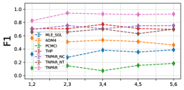
(a) Sensitivity to Range of $\alpha(\times 1e-2)$

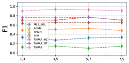
(b) Sensitivity to Range of $\mu(\times 1e-5)$

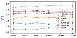
(c) Sensitivity to Sample Size

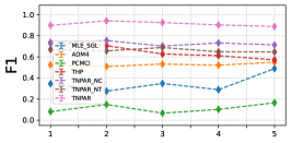
(d) Sensitivity to $\Delta$

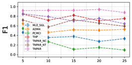
(e) Sensitivity to Num. of Event Types

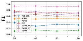
(f) Sensitivity to Num. of Nodes

Figure 3: Results on the simulated data

5.2 Baselines and Model Variants

The following Granger causal discovery methods are chosen as baseline comparisons in our experiments: PCMCI Runge (2020), MLE-SGL Xu et al. (2016), ADM4 Zhou et al. (2013), and THP Cai et al. (2022). In order to assess the components of our proposed method, we also introduce two variants of our method, namely TNPAR_NT and TNPAR_NC. Specifically, TNPAR_NT is a variant that does not incorporate topological information, while TNPAR_NC is a version that excludes both the acyclicity and sparsity regularized terms from the loss function. Detailed information about the baseline methods can be found in Appendix C.

5.3 Results on Simulated Data

The F1 scores of different methods on the simulated data are depicted in Fig. 3. Due to space limitations, results pertaining to Precision, Recall, SHD, and SID on the simulated data can be found in Appendix D.

When compared with the results of PCMCI, ADM4, and MLE_SGL (which do not consider the topological network behind the event sequences), both TNPAR and THP achieve superior performance across all cases. These results suggest that incorporating the topological network assists in learning Granger causality. As can be seen from Fig. 3, TNPAR and its variants significantly outstrip other baselines under most settings, demonstrating the efficacy of the amortized inference technique that treats Granger causal structure as a latent variable.

Across varying parameters $\alpha$, $\mu$, and $\Delta$, the F1 scores of the TNPAR algorithm markedly exceed those of other methods. These results signify that our method is relatively insensitive to the parameters of the generation process, validating the capability of the TNPAR model to effectively model the generation process of event sequences. Under conditions with varying sample sizes, or changing numbers of event types or nodes, the TNPAR algorithm achieves the highest F1 scores, illustrating the relative robustness of the TNPAR algorithm, attributable to its foundation in the neural point process. Even in instances with small sample sizes or high dimensional event types, the TNPAR algorithm still outperforms other methods, corroborating the effectiveness and robustness of TNPAR.

Of all the baseline methods, THP yields the best results since it considers the topological network underlying the event sequences. In comparison to PCMCI, both ADM4 and MLE_SGL methods perform better because they incorporate a sparsity constraint, something PCMCI does not consider.

5.4 Results on Metropolitan Cellular Network Alarm Data

The experimental results of all algorithms on real-world data are presented in Table 1. From these results, it can be seen that the models incorporated the topological network (including TNPAR, TNPAR_NC, THP) outperform that those rely on the i.i.d. assumption. Specifically, the F1 score of TNPAR is higher than that of THP, demonstrating that the TNPAR algorithm can achieve the best trade-off between Precision and Recall without needing a prior distribution assumption. Although the Precision of TNPAR is marginally lower than that of THP, PCMCI, and ADM4, TNPAR exhibits the highest Recall. These results indicate that TNPAR is relatively insensitive to the weak Granger causal strength between event types, which accounts for the slightly higher SHD of TNPAR compared to other baselines. Moreover, TNPAR attains the best SID relative to other methods. These results underscore TNPAR’s superior capability for causal inference Peters and Bühlmann (2015).

Table 1: Result on real-world data

Algorithm	Precision	Recall	F1	SID	SHD
MLE_SGL	0.39285	0.11702	0.18032	263	100
ADM4	0.49230	0.34042	0.40251	292	95
PCMCI	0.46774	0.30851	0.37179	306	102
THP	0.57894	0.35106	0.43708	266	85
TNPAR_NT	0.30830	0.48271	0.37593	257.00	150.41
TNPAR_NC	0.40893	0.60382	0.48651	271.33	123.49
TNPAR	0.45690	0.64563	0.53509	241.55	105.45

5.5 Ablation Study

Ablation experiments were conducted on both simulated and real-world data to assess the effectiveness of incorporating topological information and regularization in TNPAR. The experimental results generally reveal a significant improvement in the performance of TNPAR compared to both TNPAR_NT and TNPAR_NC. These results underscore the importance of incorporating topological information, as well as acyclic and sparse regularization. Additionally, in most instances, both TNPAR_NT and TNPAR_NC perform comparably to THP, despite the fact that the THP fully leverages topological information and sparsity constraints. These results demonstrate the robustness of the TNPAR algorithm.

5.6 Case Study

In the real-world data experiment, our method successfully infers the Granger causality across the nodes of the topological network, aligning with experts’ knowledge. From the results, we observe that the count of causal edges diminishes as the geodesic distance, denoted as $k$, increases. This finding aligns with our intuition that certain events are influenced solely by their node. For instance, the causal relationship $BD\_STATUS\rightarrow TU\_AIS$ is only valid for $k=0$. Here, $BD\_STATUS$ represents a device disconnecting from a node, and $TU\_AIS$ signifies that some tasks running on this node have been disrupted. Another notable discovery is that certain edges exclusively transit across nodes, suggesting that these event types are triggered only by their neighbors. Consider, for example, consider $ETH\_LINK\_DOWN\rightarrow MW\_LOF$, where $ETH\_LINK\_DOWN$ denotes an error on the Ethernet interface in a downstream node, and $MW\_LOF$ indicates disconnection of an upstream node.

6 Conclusion

In this paper, we present a Granger causal discovery algorithm for topological event sequences. Harnessing the pre-existing topological network and regarding the causal structure as a latent variable, we devise a method to tackle the non-i.i.d. challenge in causal discovery. This approach also addresses the complexity of unified modeling of the topological network and latent causal structure. Specifically, we first propose a comprehensive topological neural Poisson auto-regressive model to capture the generation process of topological event sequences. Subsequently, we employ amortized inference to infer the latent Granger causal structure. Lastly, we integrate these two stages into a unified likelihood function that can be optimized through an end-to-end solution. Experimental results from both simulation and real-world data corroborate the efficacy of our proposed method.

References

- Babu and Feigelson [1996] Gutti Jogesh Babu and Eric D Feigelson. Spatial point processes in astronomy. Journal of Statistical Planning and Inference, 50(3):311–326, 1996.
- Bhattacharjya et al. [2018] Debarun Bhattacharjya, Dharmashankar Subramanian, and Tian Gao. Proximal graphical event models. Advances in Neural Information Processing Systems, 31, 2018.
- Bouttier et al. [2003] Jérémie Bouttier, Philippe Di Francesco, and Emmanuel Guitter. Geodesic distance in planar graphs. Nuclear physics B, 663(3):535–567, 2003.
- Brillinger [1994] David R Brillinger. Time series, point processes, and hybrids. Canadian Journal of Statistics, 22(2):177–206, 1994.
- Cai et al. [2022] Ruichu Cai, Siyu Wu, Jie Qiao, Zhifeng Hao, Keli Zhang, and Xi Zhang. Thps: Topological hawkes processes for learning causal structure on event sequences. IEEE Transactions on Neural Networks and Learning Systems, 2022.
- Chen et al. [2020] Wei Chen, Ruichu Cai, Zhifeng Hao, Chang Yuan, and Feng Xie. Mining hidden non-redundant causal relationships in online social networks. Neural Computing and Applications, 32(11):6913–6923, 2020.
- Chen et al. [2021] Ricky T. Q. Chen, Brandon Amos, and Maximilian Nickel. Neural spatio-temporal point processes. In International Conference on Learning Representations, 2021.
- Cox [1955] David R Cox. Some statistical methods connected with series of events. Journal of the Royal Statistical Society: Series B (Methodological), 17(2):129–157, 1955.
- Cybenko [1989] George Cybenko. Approximation by superpositions of a sigmoidal function. Mathematics of Control, Signals and Systems, 2(4):303–314, 1989.
- Eichler et al. [2017] Michael Eichler, Rainer Dahlhaus, and Johannes Dueck. Graphical modeling for multivariate hawkes processes with nonparametric link functions. Journal of Time Series Analysis, 38(2):225–242, 2017.
- Ertekin et al. [2015] Şeyda Ertekin, Cynthia Rudin, and Tyler H McCormick. Reactive point processes: A new approach to predicting power failures in underground electrical systems. The Annals of Applied Statistics, 9(1):122–144, 2015.
- Gershman and Goodman [2014] Samuel Gershman and Noah Goodman. Amortized inference in probabilistic reasoning. In Annual Meeting of the Cognitive Science Society, volume 36, 2014.
- Granger [1969] Clive WJ Granger. Investigating causal relations by econometric models and cross-spectral methods. Econometrica: Journal of the Econometric Society, pages 424–438, 1969.
- Gunawardana and Meek [2016] Asela Gunawardana and Chris Meek. Universal models of multivariate temporal point processes. In Artificial Intelligence and Statistics, pages 556–563, 2016.
- Hastie et al. [2009] Trevor Hastie, Robert Tibshirani, Jerome H Friedman, and Jerome H Friedman. The elements of statistical learning: data mining, inference, and prediction, volume 2. Springer, 2009.
- Hawkes [1971] Alan G Hawkes. Spectra of some self-exciting and mutually exciting point processes. Biometrika, 58(1):83–90, 1971.
- Isham and Westcott [1979] Valerie Isham and Mark Westcott. A self-correcting point process. Stochastic processes and their applications, 8(3):335–347, 1979.
- Jang et al. [2017] Eric Jang, Shixiang Gu, and Ben Poole. Categorical reparameterization with gumbel-softmax. In International Conference on Learning Representations, 2017.
- Kingma and Ba [2015] Diederik P Kingma and Jimmy Ba. Adam: A method for stochastic optimization. In International Conference on Learning Representations, 2015.
- Li et al. [2021] Zijian Li, Ruichu Cai, Tom ZJ Fu, and Kun Zhang. Transferable time-series forecasting under causal conditional shift. arXiv preprint arXiv:2111.03422, 2021.
- Mijatovic et al. [2021] Gorana Mijatovic, Yuri Antonacci, Tatjana Loncar-Turukalo, Ludovico Minati, and Luca Faes. An information-theoretic framework to measure the dynamic interaction between neural spike trains. IEEE Transactions on Biomedical Engineering, 68(12):3471–3481, 2021.
- Othmer et al. [1988] Hans G Othmer, Steven R Dunbar, and Wolfgang Alt. Models of dispersal in biological systems. Journal of Mathematical Biology, 26(3):263–298, 1988.
- Peters and Bühlmann [2015] Jonas Peters and Peter Bühlmann. Structural intervention distance for evaluating causal graphs. Neural Computation, 27(3):771–799, 2015.
- Powers [2011] David Powers. Evaluation: From precision, recall and f-measure to roc, informedness, markedness & correlation. Journal of Machine Learning Technologies, 2(1):37–63, 2011.
- Runge [2020] Jakob Runge. Discovering contemporaneous and lagged causal relations in autocorrelated nonlinear time series datasets. In Conference on Uncertainty in Artificial Intelligence, pages 1388–1397, 2020.
- Shchur et al. [2021] Oleksandr Shchur, Ali Caner Türkmen, Tim Januschowski, and Stephan Günnemann. Neural temporal point processes: A review. In International Joint Conference on Artificial Intelligence, pages 4585–4593, 2021.
- Shojaie and Fox [2022] Ali Shojaie and Emily B Fox. Granger causality: A review and recent advances. Annual Review of Statistics and Its Application, 9:289–319, 2022.
- Spirtes et al. [2000] Peter Spirtes, Clark N Glymour, Richard Scheines, and David Heckerman. Causation, prediction, and search. MIT press, 2000.
- Stoyan et al. [2013] Dietrich Stoyan, Wilfrid S Kendall, Sung Nok Chiu, and Joseph Mecke. Stochastic geometry and its applications. John Wiley & Sons, 2013.
- Tank et al. [2018] Alex Tank, Ian Covert, Nicholas Foti, Ali Shojaie, and Emily Fox. Neural granger causality for nonlinear time series. Stat, 1050:16, 2018.
- Vuković and Thalmann [2022] Matej Vuković and Stefan Thalmann. Causal discovery in manufacturing: A structured literature review. Journal of Manufacturing and Materials Processing, 6(1):10, 2022.
- Wu et al. [2022] Peng Wu, Haoxuan Li, Yuhao Deng, Wenjie Hu, Quanyu Dai, Zhenhua Dong, Jie Sun, Rui Zhang, and Xiao-Hua Zhou. On the opportunity of causal learning in recommendation systems: Foundation, estimation, prediction and challenges. IJCAI, 2022.
- Xiao et al. [2019] Shuai Xiao, Junchi Yan, Mehrdad Farajtabar, Le Song, Xiaokang Yang, and Hongyuan Zha. Learning time series associated event sequences with recurrent point process networks. IEEE Transactions on Neural Networks and Learning Systems, 30(10):3124–3136, 2019.
- Xu et al. [2016] Hongteng Xu, Mehrdad Farajtabar, and Hongyuan Zha. Learning granger causality for hawkes processes. In International Conference on Machine Learning, pages 1717–1726, 2016.
- Yu et al. [2019] Yue Yu, Jie Chen, Tian Gao, and Mo Yu. Dag-gnn: Dag structure learning with graph neural networks. In International Conference on Machine Learning, pages 7154–7163, 2019.
- Zhang et al. [2018] Cheng Zhang, Judith Bütepage, Hedvig Kjellström, and Stephan Mandt. Advances in variational inference. IEEE Transactions on Pattern Analysis and Machine Intelligence, 41(8):2008–2026, 2018.
- Zhang et al. [2020] Wei Zhang, Thomas Panum, Somesh Jha, Prasad Chalasani, and David Page. Cause: Learning granger causality from event sequences using attribution methods. In International Conference on Machine Learning, pages 11235–11245, 2020.
- Zhou et al. [2013] Ke Zhou, Hongyuan Zha, and Le Song. Learning social infectivity in sparse low-rank networks using multi-dimensional hawkes processes. In Artificial Intelligence and Statistics, pages 641–649, 2013.