On finding 2-cuts and 3-edge-connected components in parallel
Abstract
Given a connected undirected multigraph (a graph that may contain parallel edges), the algorithm of [19] finds the 3-edge-connected components of in linear time using an innovative graph contraction technique based on a depth-first search. In [21], it was shown that the algorithm can be extended to produce a Mader construction sequence for each 3-edge-connected component, a cactus representation of the 2-cuts (cut-pairs) of each 2-edge-connected component of , and the 1-cuts (bridges) at the same time. In this paper, we further extend the algorithm of [19] to generate the 2-cuts and the 3-edge-connected components of simultaneously in linear time by performing only one depth-first search over the input graph. Previously known algorithms solve the two problems separately in multiple phases.
Keywords: 3-edge-connectivity, 3-edge-connected component, 2-cut, cut pair, 1-cut, bridge, depth-first search.
1 Introduction
3-edge-connectivity is a graph-theoretic problem that is useful in a variety of apparently unrelated areas such as editing cluster and aligning genome in bioinformatics [3, 16], solving the -irreducibility of Feynman diagram in physics and quantum chemistry [2, 9], placing monitors on the edges of a network in flow networks [1], spare capacity allocation [11], layout decomposition for multiple patterning lithography [5, 10], and the traveling salesman problem [8]. The problem calls for determining the 2-cuts and the 3-edge-connected components (abbreviated 3ecc) of a connected undirected graph. A number of linear-time algorithms for 3-edge-connectivity have been proposed [6, 13, 17, 19, 20]. An empirical experiential study reported in [14] shows that [20] has the best performance in determining the 2-cuts while [19] has the best performance in determining the 3eccs. Both algorithms are simple in that they traverse the input graph once to accomplish their task. Notice that [19] does not determine the 2-cuts while [20] needs to make another traversal over the graph after the 2-cuts are removed and some new edges are added to determine the 3eccs. Recently, Georgiadis et al. [7] presented an algorithm for finding the 2-cuts and conducted an experimental study showing that its empirical performance outperforms that of [20]. They did not address the 3ecc problem. In this article, we show that the 3ecc algorithm of [19] can be easily modified to determine the 2-cuts in parallel with the 3eccs by traversing the input graph only once.
2 Basic definitions
The definitions of the graph-theoretic concepts used in this article are standard and can be found in references such as [4, 18]. We only give some important definitions below.
An undirected graph is represented by , where is the vertex set and is the edge set. An edge with and as end-vertices is represented by . The graph may contain parallel edges (two or more edges sharing the same pair of end vertices). The degree of a vertex in , denoted by , is the number of edges with as an end-vertex. A path in is a sequence of alternating vertices and edges, , such that , where are distinct with the exception that and may be identical. The edges could be omitted if no confusion could occur. The path is a null path if and is a cycle if . The path is called an path with vertices and as terminating vertices and , as internal vertices. If the path is given an orientation from to , then is the source, denoted by , and is the sink, denoted by , of and the path is also represented by . The graph is connected if , there is a path in it. It is disconnected otherwise. Let be a connected graph. An edge is a 1- (or bridge) in if removing it from results in a disconnected graph. The graph is 2-edge-connected if it has no 1-cuts. A 2- (or cut-pair) of is a pair of edges whose removal results in a disconnected graph and neither edge is a bridge. A cut-edge is an edge in a cut-pair. is 3-edge-connected if it does not have 1-cut or 2-cut. A 3-edge-connected component (abbreviated ) of is a maximal subset such that , there exists three edge-disjoint paths in . A graph is a subgraph of if and . Let , the subgraph of induced by , denoted by , is the maximal subgraph of whose vertex set is . Let , denotes the graph resulting from after the edges in are removed.
It is well-known that performing a depth-first search [18] (henceforth, abbreviated ) over creates a spanning tree , called spanning tree of . is a rooted tree with , the vertex at which the begins, as the root. Every vertex is assigned a distinct integer, , called its dfs number, which is its rank of in the order the vertices are visited by the for the first time. The edges in are called tree edges and the edges not in are called back-edges. For , there is a unique tree-edge such that . Vertex is called the parent of , denoted by , while is a child of . The tree-edge is called the parent edge of and a child edge of and is denoted by or . If , we may write or . A back-edge with , is an outgoing back-edge (incoming back-edge, resp.) of (, resp.). The back-edge is denoted by or , where is the tail and is the head. If , we may write or .
. Specifically, is the smallest number of a vertex reachable from via a (possibly null) tree-path followed by a back-edge [18].
A path connecting a vertex with a vertex in the rooted is denoted by . A vertex is an ancestor of a vertex , denoted by , if and only if it lies on . Vertex is a proper ancestor of vertex , denoted by , if and . Vertex is a (proper) descendant of vertex if and only if is a (proper) ancestor of vertex . The subtree of rooted at , denoted by , is the subgraph of induced by the descendents of . The notation represents a path consisting of and . The notations , , etc. are defined similarly. If edge is a tree-edge with as the parent, we use and interchangeably. If edge is a back-edge with as the tail, we use and interchangeably.
3 Finding 2-cuts
The following are well-known facts about 2-cuts.
Lemma 3.1.
-
At most one of and is a back-edge;
-
if both and are tree-edges, then and lie on a tree-path connecting the root to a leaf;
-
if and , then while in ;
-
if is a 2-cut, then is also a 2-cut.
As an immediate consequence of Lemma 3.1, the set of all cut-edges can be partitioned into a collection of disjoint subsets called cut-edge chains, such that every two cut-edges in the same subset form a 2-cut and no two edges from different subsets form a 2-cut. By Lemma 3.1, each contains at most one back-edge. A cut-edge chain containing a back-edge is a TB-cut-edge chain. A cut-edge chain containing only tree-edges is a TT-cut-edge chain.
Let be a cut-edge chain. By Lemma 3.1, the edges in can be lined up along a root-to-leaf path in as follows:
-
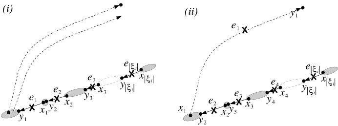
If is of TT type, the edges in can be lined up along a root-to-leaf path in in an order , where , such that (Figure 1).
-
If is of TB type, let the back-edge be . Then, the tree-edges in can be lined up along a root-to-leaf path in in an order , where , such that and (Figure 1).
The cut-edge is called the generator of [17, 20]. Hence, finding all the 2-cuts in can be reduced to determining all the cut-edge chains of .
Before explaining how to modify Algorithm 3-edge-connectivity of [19] to generate the cut-pair chains , we give the algorithm a brief review.
The key idea underlying the algorithm is to use a graph contraction operation, called absorb-eject, to gradually transform the input graph into a null (i.e., edgeless) graph of which each vertex corresponds to a distinct 3-edge-connected component of during a depth-first search.
Definition: Let and such that:
, or is not a cut-edge (which implies ).
Applying the absorb-eject operation to at results in the graph , where
, where is the set of edges incident on in and , for some . (Figure 2)
The edge is called an embodiment of the edge . In general, an embodiment of an edge is the edge itself, or an edge created to replace as a result of applying the absorb-eject operation, or an embodiment of an embodiment of .

Starting with the input graph , using the absorb-eject operation, the graph is gradually transformed so that vertices that have been confirmed to be belonging to the same are merged into one vertex, called a supervertex. Each supervertex is represented by a vertex and a set consisting of vertices that have been confirmed to be belonging to the same as . Initially, each vertex is regarded as a supervertex with . When two adjacent supervertices and are known to be belonging to the same , the absorb-eject operation is applied to have one of them, say , absorbing the other resulting in . When a supervertex containing all vertices of a is formed, it will become of degree one or two in the transformed graph (corresponding to a 1-cut or a 2-cut is found)222In [19], it is pointed out that Algorithm 3-edge-connectivity can be easily modified to handle non-2-edge-connected graphs.. Then, the absorb-eject operation is applied to an adjacent supervertex to separate (eject) the supervertex from the graph making it an isolated vertex. At the end, the graph is transformed into a collection of isolated supervertices each of which consists of the vertices of a distinct of .
During the depth-first search, at each vertex , when the adjacency list of is completely processed, let be the graph to which has been transformed at that point in time. The subtree of rooted at , , has been transformed into a path of supervertices in , , called the -path, and a set of isolated supervertices each of which corresponds to a residing in . The -path has the properties summarised in the following lemma.
Lemma 3.2.
[Lemma 6 of [19]] Let and is the graph to which has been transformed at that point in time (Figure 3).
-
and ;
-
for each back-edge in , (i.e. lies on the tree-path);
-
in such that .
Specifically, on the -path, the degree of every supervertex is at least three except that of , there is no back-edge connecting two supervertices on the -path, and the supervertex has an outgoing back-edge reaching the vertex whose dfs number is .
The -path is constructed as follows. Initially, the -path is the null path which is the current -path, and . When the dfs backtracks from a child , let be the -path, and be the graph to which has been transformed at that point in time.
If , then is a 1-cut and is a of . Edge is removed making an isolated supervertex. The current -path remains unchanged.
If , then or , where , is a 2-cut implying is a of . The absorb-eject operation is applied to edge at to eject supervertex from the -path making it an isolated supervertex and the -path is shorten to in the former case or vanishes in the latter case. Furthermore, if , then the vertices in the supervertices on the -path must all belong to the same as . The supervertices are thus absorbed by through a sequence of absorb-eject operations. if , then the vertices in the supervertices on the current -path must all belong to the same as ; the supervertices are thus absorbed by . Moreover, is updated to , and the -path after extended to include becomes the current -path, if is not ejected. If is ejected, then the -path after extended to include becomes the current -path, if exists, and is the null path , otherwise.
When an outgoing back-edge of , , with is encountered, vertex absorbs the current -path because all the supervertices on it belong to the same as ; and the current -path are then updated to and the null path , respectively.
When an incoming back-edge of , , is encountered, if such that on the current -path, the vertices in , must all belong to the same as . The supervertices are thus absorbed by (Property of the -path thus holds) and the current -path is shortened to .
When the adjacency list of is completely processed, if , the current -path becomes the -path, and the depth-first search backtracks to the parent vertex of . Otherwise, the input graph has been transformed into a collection of isolated supervertices each of which contains the vertices of a distinct of . A complete example is given in [19], pp.132-133.
During an execution of the algorithm, when the depth-first search backtracks from a vertex to the parent vertex , if , then is a 3ecc, and or is the corresponding 2-cut. Unfortunately, the 2-cut is not in , but in the transformed graph . Specifically, the corresponding 2-cut in is , such that or is an embodiment of . We shall show that the cut-edge can be easily determined as follows:
if the 2-cut in is , the corresponding 2-cut in is .
if the 2-cut in is , the corresponding 2-cut in is , where is the unique vertex such that and .
Lemma 3.3.
-
if is a tree-edge , then is a 2-cut in if and only if there does not exist a back-edge such that either;
(a) is a descendant of and not of while is an ancestor of , or
(b) is a descendant of while is a descendant of and not of .
-
If is a back-edge , then is a 2-cut in if and only if there does not exist a back-edge such that and is a descendant of while is an ancestor of .
Lemma 3.4.
During the depth-first search, when the search backtracks from a vertex to its parent vertex , Let be the -path.
If , and
-
is the 2-cut. Then the corresponding 2-cut in is ;
-
is the 2-cut (i.e., ). Then the corresponding 2-cut in is , where is the unique edge such that , and .
Proof:
-
The -path contains and implies that there is a - path in . Since remains on the -path when the depth-first search backtracks from to , there does not exist a back-edge such that is a descendant of while is a descendant of and not of ; otherwise, let be one that has closest to , then would have been absorbed by vertex when became the current vertex of the . Similarly, there does not exist a back-edge such that is a descendant of and not of while is an ancestor of ; otherwise, would have an incident edge which is an embodiment of when the depth-first search backtracks from to , implying , which contradicts the assumption . Hence, by Lemma 3.3, is the 2-cut corresponding to in .
Based on Lemma 3.4, we determine the cut-edge that forms a 2-cut with in as follow:
-
To determine , we have to know the parent vertex of every vertex in . The parent vertex of is if the depth-first search advances from to . This information can be stored in an array , where (undefined).
-
During the depth-first search, at each vertex where such that , let and . Clearly, can be determined in parallel with . The edge is a potential TB-cut-edge chain generator.
When a vertex absorbs a section of its current -path on which is the last vertex, is replaced by its embodiment in the resulting graph. By letting , can be retrieved as if needed. The value is transmitted upwards in this way, until a vertex is reached, where . Then is a 2-cut, where is the embodiment of in , Then, as , can be retrieved through and the corresponding 2-cut in is . After is ejected, if , then , because still has the potential to form new 2-cuts with other edges in . Otherwise, and become irrelevant as can no longer form 2-cuts with other edges.
The following is a pseudo-code of the modified algorithm. For clarity, the new instructions for generating the 2-cuts are marked by . The following variables are used to stored the cut-edge chains:
-
•
: a TT-cut-edge chain whose generator is ,
-
•
: a TB-cut-edge chain whose generator is .
When a vertex is ejected, Procedure Gen- is called to add the cut-edge to if both cut-edges are tree-edges, where is the vertex following in the -path before was ejected, or to , otherwise. In the latter case, is transferred to if . Procedure Absorb-path is called to absorb the current -path or a -path. Procedure Absorb-path is called when vertex absorbs a section of the current -path.
In [19], , are calculated implicitly. We calculate them explicitly based on [15]. For clarity, although we include the instructions for generating the s, we do not involve them in our discussion as their correctness is covered in [19]. we also excluded the instructions for handling parallel edges. They can be accounted for as follows:
Initially, , . When is the current vertex of the dfs, on encountering the edge , where , for the first time, and the edge is skipped. For each subsequent , implies that the edge is to be processed as an outgoing back-edge of .
Algorithm 3-edge-connectivity
Input: A connected undirected multigraph ;
Output:
begin
for each do
; // the TT-cut-edge chain with as the generator
; // the TB-cut-edge chain with as the generator
; // initialize the potential TB-type generator attached to with self-loop
; // to store the 1-cuts
; // number for next vertex
3-edge-connect;
end.
Procedure 3-edge-connect // is the parent of
begin
; ; ;
; // initialize the -path to
1 for each in do // scan the adjacency list of
; // found a new edge incident on ; update
1.1 if then // is unvisited
3-edge-connect; // advances to
; // update
1.1.1 if then // found a 1-cut or 2-cut
Gen- // generate the 1-cut or 2-cut
1.1.2 if then
; // save the current -path and attach the -path to
Absorb-path(); // absorbs the -path
; // restore the current -path
else
; // update
Absorb-path; // absorbs the current -path
; // attach the -path to to form the new current -path
1.2 else if then // an outgoing back-edge
if then
Absorb-path; // absorbs the current -path
; ; // the new current -path is
; ; // potential generator
1.3 else // an incoming back-edge
; // update
Absorb-subpath; // absorbs a section of the current -path
end.
Procedure Gen- begin
if then
; // add to the 1-cut set
; // eject
else //
if () then // , i.e., the 2-cut involves a back-edge.
if () then
; // start a TB-cut-edge chain
with generator
else ; // append to
; // , i.e., the -path vanishes after ejecting
if then ;
else if () then
; //start a TT-cut-edge chain
with generator
else ; // append to
; // eject : ;
output; // output the 3-edge-connected component
end.
Procedure Absorb-path
begin
;
while do
;
;
;
end.
Procedure Absorb-subpath
begin
;
while do // is a descendant of
;
;
;
;
;
end.
Lemma 3.5.
Let . When the adjacency list of is completely processed, let the -path be .
-
For each cut-edge chain , where or , , such that , for some ,
-
If . then ;
-
If . then ;
-
such that and , where , or .
Proof: By induction on the height of in .
At a leaf , since for any cut-edge chain, Condition vacuously holds.
Since and is updated accordingly within Instruction 1.2 whenever the condition is detected, when the depth-first search back-tracks from , and such that and . Condition thus holds.
At an internal vertex , on encountering a vertex in the adjacency list, if is unvisited, the advances to . when the backtracks from , if , is a 1-cut as its removal disconnects from . Procedure Gen-CS is invoked to add to the collection of 1-cuts, .
Let be a cut-edge chain whose generator is attached to (meaning the generator is an edge in or its tail is a vertex of ) such that , for some . Since is a 1-cut which is not a cut-edge, which implies that . Since the induction hypothesis applies to , Condition holds for . Moreover, as , remains unchanged. Condition remains valid.
If , Procedure Gen-CS is invoked.
the -path is , (i.e., ). Then, by Lemma 3.4, is the 2-cut, and the corresponding 2-cut in is , where is the unique edge such that and . By the induction hypothesis, Condition holds for which implies that such that and , where . By the uniqueness of , which implies that and . Hence, is the corresponding 2-cut in . Clearly, . If , then and . Therefore, is correctly added to . If , then for some . By the induction hypothesis, Condition holds for which implies that . Therefore, is correctly appended to . Notice that because .
If , then becomes the current -path, and , . Condition holds. If , then as the current -path and remain unchanged, Condition continues to hold.
is a 2-cut (i.e., the -path is , for some ) in . By Lemma 3.4, the corresponding 2-cut in is . Clearly, . If , then and . Therefore, is correctly added to . If , then for some . By the induction hypothesis, Condition holds for which implies that . Therefore, is correctly appended to .
If , then as the current -path remains unchanged, Condition still holds. If , then after ejecting vertex and including edge , becomes the current -path and . Since Condition holds for the -path by the induction hypothesis, the condition holds for the current -path. If , then as the current -path remains unchanged, Condition still holds.
If , the argument that Condition holds is similar to the above cases, but much simpler. If , then as the current -path remains unchanged, Condition still holds. If , then after including the edge , becomes the current -path and . Since Condition holds for the -path by the induction hypothesis, the condition thus holds for the current -path.
If is an outgoing back-edge of , , and if , then the current -path becomes , , and , Condition thus holds. If , as the current -path remains unchanged, Condition continue to hold. Since the back-edge does not involve any cut-edge chain satisfying , for some , Condition holds vacuously.
If is an incoming back-edge of , , Procedure Absorb-subpath is invoked. Since the absorption of the section of by does not affect Condition , the condition continues to hold. Moreover, if , does not absorb . Condition still holds. If , then vanishes, but when the while loop is executed for the last time, ensures that Condition holds.
When the adjacency list of is completely processed, Conditions and hold for . The lemma thus follows.
Theorem 3.6.
Algorithm 3-edge-connectivity generates all the 1-cuts, and all the 2-cuts represented by cut-edge chains for each of the 2-edge-connected components of the input graph in time.
Proof: Algorithm 3-edge-connectivity terminates execution when the adjacency list of the root is completely processed. Since for every cut-edge chain , by Lemma 3.5, all cut-edge chains are correctly computed and are kept in their corresponding or .
The time complexity follows from the fact that the time complexity of Algorithm 3-edge-connectivity of [19] is , and the new instructions increase the run time by a constant factor only.
4 Summary
We presented a linear-time algorithm that generates the 2-cuts, the 3-edge-connected components, and the 1-cuts of a connected undirected multigraph simultaneously by performing only one depth-first search over the input graph. The algorithm is conceptually simple and is based on the algorithm of [19]. Our future work is to perform an empirical study of the performances of our algorithm and the algorithm of Georgiadis et al. [7] for generating 2-cuts. Although Georgiadis et al. [7] does not address the 3-edge-connected component problem, their 2-cut algorithm provides a basis for solving the problem: determine the 2-cuts of the input graph ; remove the cut-edges from ; for each cut-edge chain with a tree-edge generator, add a new edge [17]; determine the connected components of the resulting graph which are the 3ecc of . This multi-pass algorithm should run slower than our one-pass 3ecc algorithm in practice.
References
- [1] Chin F. Y-L., Chrobak M., Yan L., “Algorithms for Placing Monitors in a Flow Network,” AAIM 2009, San Francisco, CA, June 15-17, 2009, LNCS 5564, 114-128 (2009).
- [2] Corcoran J.N., Schneider U., Schttler H.-B., “Perfect Stochastic Summation in High Order Feynman Graph Expansions,” Int. J. Mod. Phys. C, 2006, Vol. 17 (11), 1527-1549.
- [3] Dehne F., Langston M. A., Luo X., Pitre S., Shaw P., Zhang Y., “The Cluster Editing Problem: Implementations and Experiments,” IWPEC 2006, Zuerich, September 2006.
- [4] Even, S.: Graph Algorithms. Computer Science Press, Potomac, MD, 1979.
- [5] Fang S., Chang Y., Chen W., “A novel layout decomposition algorithm for triple patterning lithography,” in Proceedings of the 49th Annual Design Automation Conference. ACM, 2012, pp. 1185-1190.
- [6] Galil Z., Italiano G.F., “Reducing edge connectivity to vertex connectivity”, SIGACT News 22, 1991, 57-61.
- [7] Georgiadis L., Giannis K., Italiano G., Kosinas E., “Computing vertex-edge cut-pairs and 2-edge cuts in practice,” 19th International symposium on experimental algorithms (SEA 2021), No. 20, pp.20:1-20:19.
- [8] Isoart N., Régin J.-C.., “Integration of Structural Constraints into TSP Models,” 25th International Conference on Constraint Programming, LNCS vol.11802, pp.284-299, Connecticut, USA, 2019.
- [9] Kim A.J., Li J., Eckstein M., Werner P., “Pseudoparticle vertex solver for quantum impurity models,” Physical Reviews B 106, 085124, 2022.
- [10] Kuang J., Young E., “An efficient layout decomposition approach for triple patterning lithography,” Proceedings of the 50th Annual Design Automation Conference. ACM, 2013
- [11] Liu V. Y., Tipper D., “Spare capacity allocation using shared backup path protection for dual link failures,” Computer Communications 36, 666-677, 2013.
- [12] Nadara W., Radecki M., Smulewicz M., Sokolowski M., “Determining 4-edge-connected components in linear time,” arXiv:2105.01699v1 [cs.DS] 4 May 2021.
- [13] Nagamochi H., Ibaraki T., “A linear-time algorithm for computing 3-edge-connected components in a multigraph”, Japan J. Indust. Appl. Math., vol. 9, 1992, 163-180.
- [14] Norouzi N., “A study of 3-edge-connectivity algorithms - Refinement and Implementation,” M.Sc. Thesis, School of Computer Science, University of Windsor, 2007.
- [15] Norouzi N., Tsin Y.H., “A simple 3-edge connected component algorithm revisited,” Information Processing Letters, vol. 114(1-2), 2014, 50-55.
- [16] Paten B., Diekhans M., Earl D., St. John J., Ma J., Suh B., Haussler D., “Cactus Graphs for Genome Comparisons,” RECOMB 2010, Lisbon, Portugal, April 2010, LNCS 6044, 410-425 (2010).
- [17] Taoka S., Watanabe T., Onaga K., “A linear-time algorithm for computing all 3-edge-connected components of a multigraph”, IEICE Trans. Fundamentals, vol. E75(3), 1992, 410-424.
- [18] Trajan R., “Depth-first Search and Linear Graph Algorithms,” SIAM J. COMPUT., 1 (2), June 1972.
- [19] Tsin, Y.H., “A simple 3-edge-connected component algorithm”, Theory of Computing Systems, vol. 40(2), 2007, 125-142.
- [20] Tsin, Y.H., “Yet another optimal algorithm for 3-edge-connectivity”, Journal of Discrete Algorithms, vol. 7(1), 2009, 130-146.
- [21] Tsin, Y.H., ”A simple certifying algorithm for 3-edge-connectivity,” Theoretical Computer Science, 951 (2023) 113760, 1-26.