Locally Differentially Private Distributed Online Learning with Guaranteed Optimality

Ziqin Chen and Yongqiang Wang, Senior Member, IEEE The work was supported in part by the National Science Foundation under Grants ECCS-1912702, CCF-2106293, CCF-2215088, and CNS-2219487.Ziqin Chen and Yongqiang Wang are with the Department of Electrical and Computer Engineering, Clemson University, Clemson, SC 29634 USA (e-mail: ziqinc@clemson.edu; yongqiw@clemson.edu).
Abstract

Distributed online learning is gaining increased traction due to its unique ability to process large-scale datasets and streaming data. To address the growing public awareness and concern on privacy protection, plenty of private distributed online learning algorithms have been proposed, mostly based on differential privacy which has emerged as the “gold standard” for privacy protection. However, these algorithms often face the dilemma of trading learning accuracy for privacy. By exploiting the unique characteristics of online learning, this paper proposes an approach that tackles the dilemma and ensures both differential privacy and learning accuracy in distributed online learning. More specifically, while ensuring a diminishing expected instantaneous regret, the approach can simultaneously ensure a finite cumulative privacy budget, even on the infinite time horizon. To cater for the fully distributed setting, we adopt the local differential-privacy framework which avoids the reliance on a trusted data curator, and hence, provides stronger protection than the classic “centralized” (global) differential privacy. To the best of our knowledge, this is the first algorithm that successfully ensures both rigorous local differential privacy and learning accuracy. The effectiveness of the proposed algorithm is evaluated using machine learning tasks, including logistic regression on the “Mushrooms” and “Covtype” datasets and CNN based image classification on the “MNIST” and “CIFAR-10” datasets.

Index Terms:
Distributed online learning, local differential privacy, instantaneous regret.

I Introduction

The modern data landscape, fueled by advances in web technologies, social media, and sensory devices, calls for evolved machine learning methods to handle the “big data” challenge [1]. Due to its unique ability to handle streaming data, online learning has emerged as an attractive paradigm to address this challenge [2]. In online learning, data are accessed and processed in a sequential manner, thereby obviating the requirement to process the entire dataset at once. This feature makes online learning algorithms particularly appealing for large-scale datasets and dynamic scenarios where data are continually generated, ranging from financial markets, social media streams, to real-time sensor interpretation [3].

Traditional online learning algorithms (e.g., [4, 5, 6]) require transmitting all data streams to a central location for processing, leading to potential security risks like information leakage or model compromises in the event of a server attack [7]. Distributed online learning algorithms mitigate these risks by dispersing data among multiple networked learners, each updating its model with local streaming data, and then sharing updates across the network for parameter synchronization (see, e.g., [8, 9, 10, 11, 12, 13, 14]). While these algorithms eliminate the need for centralized data storage and associated security risks, information leakage during parameter transmission remains a concern, particularly via unencrypted communication channels. In fact, using these shared parameters, not only can an adversary infer sensitive attributes of the original data [15], but it can also precisely reversely infer raw training data (pixel-wise accurate for images [16]). To mitigate privacy breaches in distributed online learning, one natural approach is to patch an online learning algorithm with existing privacy mechanisms. For example, partially homomorphic encryption has been employed in both our prior results as well as others’ to ensure privacy in distributed optimization [17, 18, 19]. However, such approaches suffer from heavy communication and computation overheads. Alternatively, time or spatially correlated noise-based approaches preserve privacy while maintaining accuracy by canceling out injected noise [20, 21, 22, 23, 24]. However, such approaches require each learner to have at least one neighbor not sharing information with potential adversaries, a condition that is difficult to guarantee in many multi-agent networks.

As differential privacy (DP) has been widely accepted as the standard notion of privacy [25], plenty of results have been proposed to enable differential privacy in distributed optimization/learning. Most of the results explicitly rely on a trusted curator to aggregate and publish data [26, 27, 28]. Recently, some differential-privacy solutions have been proposed for fully distributed optimization algorithms, including [29, 30, 31, 32] as well as our own prior work [33, 34]. However, since these results still use the classic “centralized” differential-privacy framework, they implicitly require that the agents mutually cooperate with each other in publishing data [35]. To ensure privacy in the scenario where an agent does not trust anyone else (including other participating agents) and aims to protect against an adversary that can observe every message shared in the network, we have to use local differential privacy (LDP), which is widely regarded as the strongest model of differential privacy [36, 37, 38, 39].

Unfortunately, the benefit of LDP comes at a great cost in utility. To the best of our knowledge, all existing differential-privacy solutions for distributed online learning either have to sacrifice learning accuracy [40, 41], or allow the cumulative privacy budget growing to infinity with time [30, 31, 42, 43], implying diminishing privacy protection as time tends to infinity. It is worth noting that our previous result on differentially private offline distributed optimization [34] manages to retain provable convergence accuracy while ensuring DP. However, it still uses the classic “centralized” DP framework, and it is unclear if the offline learning approach can be extended to the online learning scenario, where data arrive sequentially.

In this paper, we propose an LDP-distributed online learning algorithm that efficiently circumvents the trade-off between privacy and learning accuracy. Our key idea is to exploit both a decaying interaction strength (as in our prior result [34]) and the unique data patterns in online learning. We assess online learning accuracy using expected instantaneous regret, which we prove to converge to zero. The main contributions are summarized as follows:

  • We demonstrate that for both strongly convex and general convex objective functions, our proposed LDP-distributed online learning algorithm ensures that the expected instantaneous regret decreases to zero, even in the presence of persistent DP-noise variances. Moreover, in the strongly convex scenario, we further prove that the expected tracking error (the deviation between the online algorithm’s output and the optimal solution) also converges to zero. To the best of our knowledge, no such results have been reported before.

  • In addition to ensuring accurate convergence, we prove that our algorithm can simultaneously ensure rigorous LDP, even on the infinite time horizon. To our knowledge, this is the first time that both goals of LDP and provable convergence are achieved simultaneously in distributed online learning. This is in sharp contrast to existing results on differentially private distributed online learning in [30, 31, 42, 43], where the privacy budget grows to infinity when time tends to infinity.

  • Moreover, our LDP framework allows individual learners to choose heterogeneous privacy budgets in a fully distributed manner, making individual learners free to chose desired privacy strengths depending on practical needs.

  • Besides providing a theoretic approach to selecting stepsizes based on global parameters such as graph Laplacian and the global Lipschitz constant (which is common in most existing distributed online optimization algorithms [10, 11, 12]), we also provide an approach for individual learners to select stepsizes independently of any global parameters, which is more amenable to distributed implementations.

  • We evaluated the performance of our approach using several benchmark machine learning datasets, including the “Mushrooms” and “Covtype” datasets for logistic regression and the “MNIST” and “CIFAF-10” datasets for CNN based image classification. The results corroborate the effectiveness of our approach. Notably, compared to existing DP-distributed learning/optimization methods in [42, 43, 29], our algorithm demonstrates higher learning and testing accuracies.

The organization of the paper is as follows. Sec. II introduces the problem formulation and definitions for LDP. Sec. III presents an LDP-distributed online learning algorithm and discusses its computational complexity. Sec. IV analyzes the learning accuracy of the proposed algorithm. Sec. VI establishes the LDP guarantees. Sec. VII presents experimental results on benchmark datasets. Sec. VIII concludes the paper.

Notations: We use nsuperscript𝑛\mathbb{R}^{n} to denote the n𝑛n-dimensional Euclidean space. Insubscript𝐼𝑛I_{n} represents the identity matrix of dimension n𝑛n and 𝟏nsubscript1𝑛\mathbf{1}_{n} represents the n𝑛n-dimensional column vector with all entries equal to 111. In both cases we suppress the dimension subscript when it is clear from the context. The inner product is denoted by ,\langle\cdot,\cdot\rangle and \|\cdot\| represents the Euclidean norm of a vector. The Kronecker product is denoted by tensor-product\otimes. The stacked column vector of vectors or scalars θ1,,θNsubscript𝜃1subscript𝜃𝑁\theta_{1},\cdots,\theta_{N} is denoted by col{θ1,,θN}colsubscript𝜃1subscript𝜃𝑁{\rm col}\{\theta_{1},\cdots,\theta_{N}\}. The transpose of a matrix A𝐴A is written as ATsuperscript𝐴𝑇A^{T}. The notation a𝑎\lceil a\rceil refers to the smallest integer no less than a𝑎a, and a𝑎\lfloor a\rfloor represents the largest integer no greater than a𝑎a. We use [m]delimited-[]𝑚[m] to denote the set {1,2,,m}12𝑚\{1,2,\cdots,m\}.

II Problem Statement

II-A Distributed online learning

In distributed online learning, each learner i,i[m]𝑖𝑖delimited-[]𝑚i,~{}i\in[m] must perform learning on streaming data that arrive sequentially. More specifically, at time instant t𝑡t, learner i𝑖i acquires data point xtisuperscriptsubscript𝑥𝑡𝑖x_{t}^{i}, which is independently and identically sampled from an unknown distribution over a sample space 𝒳isubscript𝒳𝑖\mathcal{X}_{i}. Using the model parameter θtisuperscriptsubscript𝜃𝑡𝑖\theta_{t}^{i} learned from data prior to time t𝑡t, which is usually constrained in a convex subset ΘΘ\Theta of nsuperscript𝑛\mathbb{R}^{n}, learner i𝑖i predicts a label y^tisuperscriptsubscript^𝑦𝑡𝑖\hat{y}_{t}^{i} for data xtisuperscriptsubscript𝑥𝑡𝑖x_{t}^{i} acquired at time t𝑡t. When the true label ytisuperscriptsubscript𝑦𝑡𝑖y_{t}^{i}\in\mathbb{R} is revealed, the learner experiences a loss l(θti,ξti)𝑙superscriptsubscript𝜃𝑡𝑖superscriptsubscript𝜉𝑡𝑖l(\theta_{t}^{i},\xi_{t}^{i}), where ξti=(xti,yti)superscriptsubscript𝜉𝑡𝑖superscriptsubscript𝑥𝑡𝑖superscriptsubscript𝑦𝑡𝑖\xi_{t}^{i}=(x_{t}^{i},y_{t}^{i}) resides in 𝒟i=𝒳i×subscript𝒟𝑖subscript𝒳𝑖\mathcal{D}_{i}=\mathcal{X}_{i}\times\mathbb{R}. The loss prompts learner i𝑖i to adjust its model parameter θtisuperscriptsubscript𝜃𝑡𝑖\theta_{t}^{i}. The goal of distributed online learning is to let m𝑚m learners cooperatively find a common optimal parameter, based on sequentially acquired streaming data, for the following stochastic optimization problem:

minθΘF(θ):=1mi=1mfi(θ),assignsubscriptmin𝜃Θ𝐹𝜃1𝑚superscriptsubscript𝑖1𝑚subscript𝑓𝑖𝜃\text{min}_{\theta\in\Theta}\quad F(\theta):=\frac{1}{m}\sum_{i=1}^{m}f_{i}(\theta), (1)

where fi(θ)=𝔼ξi𝒟i[l(θ,ξi)]subscript𝑓𝑖𝜃subscript𝔼similar-tosuperscript𝜉𝑖subscript𝒟𝑖delimited-[]𝑙𝜃superscript𝜉𝑖f_{i}(\theta)\!=\!\mathbb{E}_{\xi^{i}\sim\mathcal{D}_{i}}\!\left[l(\theta,\xi^{i})\right] satisfies the following assumption:

Assumption 1.

(i) ΘΘ\Theta is a convex and compact subset of nsuperscript𝑛\mathbb{R}^{n} with nonempty interior.

(ii) For all i[m]𝑖delimited-[]𝑚i\in[m] and x,yΘ𝑥𝑦Θx,y\in\Theta, there exists some μ0𝜇0\mu\geq 0 such that the following inequality holds:

fi(y)fi(x)+fi(x)T(yx)+μ2xy2.subscript𝑓𝑖𝑦subscript𝑓𝑖𝑥subscript𝑓𝑖superscript𝑥𝑇𝑦𝑥𝜇2superscriptnorm𝑥𝑦2\displaystyle f_{i}(y)\geq f_{i}(x)+\nabla f_{i}(x)^{T}(y-x)+\frac{\mu}{2}\|x-y\|^{2}.

(iii) The gradients of fisubscript𝑓𝑖f_{i} is uniformly bounded, i.e., there exists some D>0𝐷0D>0, such that we have the following inequality for all θΘ𝜃Θ\theta\in\Theta:

fi(θ)D.normsubscript𝑓𝑖𝜃𝐷\|\nabla f_{i}(\theta)\|\leq D.

We consider the setting where m𝑚m learners are connected with an undirected and connected graph 𝒢=([m],)𝒢delimited-[]𝑚\mathcal{G}=([m],\mathcal{E}). Here, m𝑚m learners are represented as [m]={1,,m}delimited-[]𝑚1𝑚[m]=\{1,\cdots,m\} and their interactions are represented by edges in the set \mathcal{E}. The set of learners that can directly interact with learner i𝑖i is called the neighboring set of learner i𝑖i and is represented as 𝒩isubscript𝒩𝑖\mathcal{N}_{i}. The interaction strength is described by using a weight matrix W={wij}m×m𝑊subscript𝑤𝑖𝑗superscript𝑚𝑚W=\{w_{ij}\}\in\mathbb{R}^{m\times m}, in which wij>0subscript𝑤𝑖𝑗0w_{ij}>0 if the edge (i,j)𝑖𝑗(i,j)\in\mathcal{E} exists, and wij=0subscript𝑤𝑖𝑗0w_{ij}=0 otherwise. The weight matrix satisfies the following assumption:

Assumption 2.

The weight matrix W={wij}m×m𝑊subscript𝑤𝑖𝑗superscript𝑚𝑚W=\{w_{ij}\}\in\mathbb{R}^{m\times m} is symmetric and satisfies 𝟏TW=𝟎Tsuperscript1𝑇𝑊superscript0𝑇\mathbf{1}^{T}W=\mathbf{0}^{T}, W𝟏=𝟎𝑊10W\mathbf{1}=\mathbf{0}, and I+W𝟏𝟏Tm<1norm𝐼𝑊superscript11𝑇𝑚1\|I+W-\frac{\mathbf{1}\mathbf{1}^{T}}{m}\|<1. The eigenvalues of W𝑊W satisfy (after arranged in an increasing order) 1<δNδ2<δ1=01subscript𝛿𝑁subscript𝛿2subscript𝛿10-1<\delta_{N}\leq\cdots\leq\delta_{2}<\delta_{1}=0.

To solve for (1) with fisubscript𝑓𝑖f_{i} equal to the expected value of the loss function l(θ,ξi)𝑙𝜃superscript𝜉𝑖l(\theta,\xi^{i}), we have to know the distribution 𝒟isubscript𝒟𝑖\mathcal{D}_{i} of ξisuperscript𝜉𝑖\xi^{i}. However, in practice, the distribution 𝒟isubscript𝒟𝑖\mathcal{D}_{i} is usually unknown, which makes it impossible to directly compute 𝔼ξi𝒟i[l(θ,ξi)]subscript𝔼similar-tosuperscript𝜉𝑖subscript𝒟𝑖delimited-[]𝑙𝜃superscript𝜉𝑖\mathbb{E}_{\xi^{i}\sim\mathcal{D}_{i}}\left[l(\theta,\xi^{i})\right]. To circumvent this problem, a common approach is reformulating (1) as the following Empirical Risk Minimization (ERM) problem:

minθΘFt(θ):=1mi=1m1t+1k=0tl(θ,ξki).assignsubscriptmin𝜃Θsubscript𝐹𝑡𝜃1𝑚superscriptsubscript𝑖1𝑚1𝑡1superscriptsubscript𝑘0𝑡𝑙𝜃superscriptsubscript𝜉𝑘𝑖\text{min}_{\theta\in\Theta}\quad F_{t}(\theta):=\frac{1}{m}\sum_{i=1}^{m}\frac{1}{t+1}\sum_{k=0}^{t}l(\theta,\xi_{k}^{i}).\vspace{-0.3em} (2)

According to the law of large numbers, we have limt1t+1k=0tl(θ,ξki)=𝔼ξi𝒟i[l(θ,ξi)]subscript𝑡1𝑡1superscriptsubscript𝑘0𝑡𝑙𝜃superscriptsubscript𝜉𝑘𝑖subscript𝔼similar-tosuperscript𝜉𝑖subscript𝒟𝑖delimited-[]𝑙𝜃superscript𝜉𝑖\lim_{t\rightarrow\infty}\frac{1}{t+1}\sum_{k=0}^{t}l(\theta,\xi_{k}^{i})\!\!=\!\!\mathbb{E}_{\xi^{i}\sim\mathcal{D}_{i}}\left[l(\theta,\xi^{i})\right] almost surely, implying that the solution to (2) gradually approaches the solution to (1) as time t𝑡t tends to infinity. It is worth noting that different from the conventional ERM problem, where all data are accumulated prior to performing training, here we have to perform online training from experience as more data are observed. In addition, since ξti𝒟isuperscriptsubscript𝜉𝑡𝑖subscript𝒟𝑖\xi_{t}^{i}\in\mathcal{D}_{i} are randomly streaming data, the gradients l(θti,ξti)𝑙superscriptsubscript𝜃𝑡𝑖superscriptsubscript𝜉𝑡𝑖\nabla l(\theta_{t}^{i},\xi_{t}^{i}) are stochastic, which we assume to satisfy the following standard assumption:

Assumption 3.

The random data points {ξti}superscriptsubscript𝜉𝑡𝑖\{\xi_{t}^{i}\} are independent of each other. In addition,

(i) 𝔼[l(θti,ξti)|θti]=fi(θti)𝔼delimited-[]conditional𝑙superscriptsubscript𝜃𝑡𝑖superscriptsubscript𝜉𝑡𝑖superscriptsubscript𝜃𝑡𝑖subscript𝑓𝑖superscriptsubscript𝜃𝑡𝑖\mathbb{E}[\nabla l(\theta_{t}^{i},\xi_{t}^{i})|\theta_{t}^{i}]=\nabla f_{i}(\theta_{t}^{i}).

(ii) 𝔼[l(θti,ξti)fi(θti)2|θti]κ2𝔼delimited-[]conditionalsuperscriptnorm𝑙superscriptsubscript𝜃𝑡𝑖superscriptsubscript𝜉𝑡𝑖subscript𝑓𝑖superscriptsubscript𝜃𝑡𝑖2superscriptsubscript𝜃𝑡𝑖superscript𝜅2\mathbb{E}[\|\nabla l(\theta_{t}^{i},\xi_{t}^{i})-\nabla f_{i}(\theta_{t}^{i})\|^{2}|\theta_{t}^{i}]\leq\kappa^{2}.

(iii) 𝔼[l(x,ξti)l(y,ξti)|t]Lxy𝔼delimited-[]conditionalnorm𝑙𝑥superscriptsubscript𝜉𝑡𝑖𝑙𝑦superscriptsubscript𝜉𝑡𝑖subscript𝑡𝐿norm𝑥𝑦\mathbb{E}[\|\nabla l(x,\xi_{t}^{i})-\nabla l(y,\xi_{t}^{i})\||\mathcal{F}_{t}]\leq L\|x-y\|, where tsubscript𝑡\mathcal{F}_{t} denotes the σ𝜎\sigma-algebra generated by {ξki}0kt,i[m]subscriptsuperscriptsubscript𝜉𝑘𝑖0𝑘𝑡𝑖delimited-[]𝑚\{\xi_{k}^{i}\}_{0\leq k\leq t},~{}i\in[m].

Furthermore, given the streaming nature of data, the function Ft(θ)subscript𝐹𝑡𝜃F_{t}(\theta) in (2) varies with time, which further leads to a time-varying optimal solution θtsubscriptsuperscript𝜃𝑡\theta^{\ast}_{t}. Hence, to evaluate the quality of the parameters learned by learners through a distributed online learning algorithm at each time instant, we employ the following expected tracking error metric:

Definition 1.

(Expected tracking error) Define θtsuperscriptsubscript𝜃𝑡\theta_{t}^{*} as the optimal parameter (solution) to the optimization problem (2) at time t𝑡t. The expected tracking error is defined as the maximum expectation of the difference between the learned parameters θtisuperscriptsubscript𝜃𝑡𝑖\theta_{t}^{i} and the optimal parameter θtsuperscriptsubscript𝜃𝑡\theta_{t}^{*}, i.e.,

Vt=maxi[m]{𝔼[θtiθt2]}.subscript𝑉𝑡subscript𝑖delimited-[]𝑚𝔼delimited-[]superscriptnormsuperscriptsubscript𝜃𝑡𝑖superscriptsubscript𝜃𝑡2V_{t}=\max_{i\in[m]}\left\{\mathbb{E}\left[\|\theta_{t}^{i}-\theta_{t}^{*}\|^{2}\right]\right\}. (3)
Remark 1.

Tracking error is a widely used performance metric in online learning/optimization [44, 45, 46], particularly in scenarios with time-varying data or non-stationary environments. It quantifies the ability of an online algorithm to adapt to variations in the optimal parameter.

The defined expected tracking error evaluates the maximum expected deviation across all learners with respect to the optimal parameter. Correspondingly, to measure the maximum expected difference in objective function values (losses), we introduce the definition of expected instantaneous regret, which is defined as follows:

Definition 2.

(Expected instantaneous regret) The expected instantaneous regret measures the maximum expected loss of an online algorithm at each time t𝑡t with respect to the optimal loss, i.e.,

Rt=maxi[m]{𝔼[Ft(θti)Ft(θt)]}.subscript𝑅𝑡subscript𝑖delimited-[]𝑚𝔼delimited-[]subscript𝐹𝑡superscriptsubscript𝜃𝑡𝑖subscript𝐹𝑡superscriptsubscript𝜃𝑡R_{t}=\max_{i\in[m]}\{\mathbb{E}\left[F_{t}(\theta_{t}^{i})-F_{t}(\theta_{t}^{*})\right]\}.\vspace{-0.3em} (4)
Remark 2.

The defined expected instantaneous regret at time t𝑡t quantifies the real-time expected loss incurred by the learned parameters at time t𝑡t [47, 48]. Unlike dynamic regret, which emphasizes the accumulated error [43, 29], instantaneous regret captures the real-time performance of the online algorithm, thereby having a better fit to spatiotemporally fluctuating environments [49].

II-B Local differential privacy

Local differential privacy is a differential-privacy model for scenarios where no trusted data aggregator (curator) exists to aggregate data and execute a privacy mechanism. It is contrasted with the classic “centralized” differential privacy, where a trusted aggregator gathers all raw data and then executes a differentially private data publishing mechanism. In distributed learning and optimization, each learner maintains a local dataset and shares learned parameters with neighbors to collaboratively optimize these parameters. This information exchange has the risks of information leakage as malicious external attackers or curious neighbors might try to recover raw data from shared parameters [7, 15]. To protect the privacy of all learners, we adopt LDP to address the most severe scenario: all communication channels can be compromised by malicious attackers and no learners are trustworthy. Consequently, not only does our LDP-based approach deter external adversaries from extracting raw data through shared information, but it also shields against neighboring curious learners within the network.

To facilitate privacy analysis, we need the definition of adjacency of local datasets:

Definition 3.

(Adjacency). Given two local datasets 𝒟i={ξ1i,ξ2i,,ξTi}subscript𝒟𝑖superscriptsubscript𝜉1𝑖superscriptsubscript𝜉2𝑖superscriptsubscript𝜉𝑇𝑖\mathcal{D}_{i}=\{\xi_{1}^{i},\xi_{2}^{i},\cdots,\xi_{T}^{i}\} and 𝒟i={ξ1i,ξ2i,,ξTi},i[m]formulae-sequencesuperscriptsubscript𝒟𝑖superscriptsuperscriptsubscript𝜉1𝑖superscriptsuperscriptsubscript𝜉2𝑖superscriptsuperscriptsubscript𝜉𝑇𝑖for-all𝑖delimited-[]𝑚{\mathcal{D}_{i}}^{\prime}=\{{\xi_{1}^{i}}^{\prime},{\xi_{2}^{i}}^{\prime},\cdots,{\xi_{T}^{i}}^{\prime}\},~{}\forall i\in[m], 𝒟isubscript𝒟𝑖\mathcal{D}_{i} is said to be adjacent to 𝒟isuperscriptsubscript𝒟𝑖{\mathcal{D}_{i}}^{\prime} if there exists a time instant k{0,,T}𝑘0𝑇k\in\{0,\cdots,T\} such that ξkiξkisuperscriptsubscript𝜉𝑘𝑖superscriptsuperscriptsubscript𝜉𝑘𝑖\xi_{k}^{i}\neq{\xi_{k}^{i}}^{\prime} while ξti=ξtisuperscriptsubscript𝜉𝑡𝑖superscriptsuperscriptsubscript𝜉𝑡𝑖\xi_{t}^{i}={\xi_{t}^{i}}^{\prime} for all tk,t{0,,T}formulae-sequence𝑡𝑘𝑡0𝑇t\neq k,~{}t\in\{0,\cdots,T\}.

It can be seen that 𝒟isubscript𝒟𝑖\mathcal{D}_{i} is adjacent to 𝒟isuperscriptsubscript𝒟𝑖{\mathcal{D}_{i}}^{\prime} if and only if 𝒟isubscript𝒟𝑖\mathcal{D}_{i} and 𝒟isuperscriptsubscript𝒟𝑖{\mathcal{D}_{i}}^{\prime} differ in a single entry while all other entries are the same. We use Adj(𝒟i,𝒟i)Adjsubscript𝒟𝑖superscriptsubscript𝒟𝑖\text{Adj}(\mathcal{D}_{i},{\mathcal{D}_{i}}^{\prime}) to denote this adjacent relationship.

Given a distributed online learning problem (2), we denote the execution of an online algorithm by learner i,i[m]𝑖𝑖delimited-[]𝑚i,~{}i\in[m] as 𝒜isubscript𝒜𝑖\mathcal{A}_{i}. Learner i𝑖i injects Laplace noise to all its shared messages to achieve privacy protection. We use Lap(νi)Lapsubscript𝜈𝑖\text{Lap}(\nu_{i}) to denote Laplace distribution with parameter νi>0subscript𝜈𝑖0\nu_{i}>0, featuring a probability density function 12νie|x|νi12subscript𝜈𝑖superscript𝑒𝑥subscript𝜈𝑖\frac{1}{2\nu_{i}}e^{\frac{-|x|}{\nu_{i}}}. Lap(νi)Lapsubscript𝜈𝑖\text{Lap}(\nu_{i}) has a mean of zero and a variance of 2νi22superscriptsubscript𝜈𝑖22\nu_{i}^{2}.

Now we are in a position to present the definition of LDP:

Definition 4.

(Local differential privacy). Let 𝒜i(𝒟i,θi)subscript𝒜𝑖subscript𝒟𝑖superscript𝜃𝑖\mathcal{A}_{i}(\mathcal{D}_{i},\theta^{-i}) denote the output of learner i𝑖i under a distributed learning algorithm with its local dataset 𝒟isubscript𝒟𝑖\mathcal{D}_{i} and all received information from neighbors θisuperscript𝜃𝑖\theta^{-i}. Then, learner i𝑖i’s implementation 𝒜isubscript𝒜𝑖\mathcal{A}_{i} of Algorithm 1 is ϵisubscriptitalic-ϵ𝑖\epsilon_{i}-local differentially private if the following inequality always holds for any two adjacent datasets 𝒟isubscript𝒟𝑖\mathcal{D}_{i}𝒟isuperscriptsubscript𝒟𝑖{\mathcal{D}_{i}}^{\prime}:

[𝒜i(𝒟i,θi)𝒪i]eϵi[𝒜i(𝒟i,θi)𝒪i],delimited-[]subscript𝒜𝑖subscript𝒟𝑖superscript𝜃𝑖subscript𝒪𝑖superscript𝑒subscriptitalic-ϵ𝑖delimited-[]subscript𝒜𝑖superscriptsubscript𝒟𝑖superscript𝜃𝑖subscript𝒪𝑖\displaystyle\mathbb{P}[\mathcal{A}_{i}(\mathcal{D}_{i},\theta^{-i})\in\mathcal{O}_{i}]\leq e^{\epsilon_{i}}\mathbb{P}[\mathcal{A}_{i}({\mathcal{D}_{i}}^{\prime},\theta^{-i})\in\mathcal{O}_{i}], (5)

where 𝒪isubscript𝒪𝑖\mathcal{O}_{i} represents the set of all possible observations.

The parameter ϵisubscriptitalic-ϵ𝑖\epsilon_{i} measures the similarity (indistinguishability) of learner i𝑖i’s output distributions under two adjacent datasets. A smaller value of ϵisubscriptitalic-ϵ𝑖\epsilon_{i} indicates greater indistinguishability between the outputs for two adjacent datasets, implying a higher level of privacy protection.

In our definition of LDP, for learner i𝑖i, all received information from neighbors, i.e., θisuperscript𝜃𝑖\theta^{-i}, is regarded as external information and beyond its control. This is different from the classic “centralized” DP definition used in existing differentially private distributed optimization/learning approaches [29, 30, 31, 32, 33, 34], which, in the absence of a data aggregator/curator, requires participating learners to trust each other and cooperatively determine the amount of noise needed to achieve a certain level of privacy protection (privacy budget). In fact, when no data aggregator/curator exists, such a “centralized” DP framework even allows agents to cooperatively decide (like a centralized data curator) how to mask shared information [35].

III LDP-Distributed online learning algorithm

III-A Algorithm design

Our LDP-distributed online learning algorithm to solve problem (2) is summarized in Algorithm 1.

  Algorithm 1: LDP-Distributed online learning for learner i𝑖i
Initialization: θ0iΘsuperscriptsubscript𝜃0𝑖Θ\theta_{0}^{i}\in{\Theta} and i[m]={1,,m}𝑖delimited-[]𝑚1𝑚i\in[m]=\{1,\cdots,m\}. 1: For t=0,1,2,𝑡012t=0,1,2,\cdots do
2: Receive data ξti𝒟isuperscriptsubscript𝜉𝑡𝑖subscript𝒟𝑖\xi_{t}^{i}\in\mathcal{D}_{i}.
3: Using all available data up to time t𝑡t, i.e., ξki𝒟i,k[0,t]formulae-sequencesuperscriptsubscript𝜉𝑘𝑖subscript𝒟𝑖𝑘0𝑡\xi_{k}^{i}\in\mathcal{D}_{i},~{}k\in[0,t] and the current parameter θtisuperscriptsubscript𝜃𝑡𝑖\theta_{t}^{i}, learner i𝑖i computes the gradient dti(θti)1t+1k=0tl(θti,ξki)superscriptsubscript𝑑𝑡𝑖superscriptsubscript𝜃𝑡𝑖1𝑡1superscriptsubscript𝑘0𝑡𝑙superscriptsubscript𝜃𝑡𝑖superscriptsubscript𝜉𝑘𝑖d_{t}^{i}(\theta_{t}^{i})\triangleq\frac{1}{t+1}\sum_{k=0}^{t}\nabla l(\theta_{t}^{i},\xi_{k}^{i}).
5. Receive neighbors’ parameters θtj+ζtj,j𝒩isuperscriptsubscript𝜃𝑡𝑗superscriptsubscript𝜁𝑡𝑗𝑗subscript𝒩𝑖\theta_{t}^{j}+\zeta_{t}^{j},~{}j\in{\mathcal{N}_{i}}.
6. Parameter Update: θ^t+1i=θti+j𝒩iγtwij(θtj+ζtjθti)λtdti(θti),superscriptsubscript^𝜃𝑡1𝑖superscriptsubscript𝜃𝑡𝑖subscript𝑗subscript𝒩𝑖subscript𝛾𝑡subscript𝑤𝑖𝑗superscriptsubscript𝜃𝑡𝑗superscriptsubscript𝜁𝑡𝑗superscriptsubscript𝜃𝑡𝑖subscript𝜆𝑡superscriptsubscript𝑑𝑡𝑖superscriptsubscript𝜃𝑡𝑖\displaystyle\hat{\theta}_{t+1}^{i}=\theta_{t}^{i}+\sum_{j\in{\mathcal{N}_{i}}}\gamma_{t}w_{ij}(\theta_{t}^{j}+\zeta_{t}^{j}-\theta_{t}^{i})-\lambda_{t}d_{t}^{i}(\theta_{t}^{i}), (6) θt+1i=ProΘ(θ^t+1i),superscriptsubscript𝜃𝑡1𝑖subscriptProΘsuperscriptsubscript^𝜃𝑡1𝑖\displaystyle\theta_{t+1}^{i}=\text{Pro}_{\Theta}(\hat{\theta}_{t+1}^{i}), (6) where γt=γ0(t+1)usubscript𝛾𝑡subscript𝛾0superscript𝑡1𝑢\gamma_{t}\!=\!\frac{\gamma_{0}}{(t+1)^{u}} and λt=λ0(t+1)vsubscript𝜆𝑡subscript𝜆0superscript𝑡1𝑣\lambda_{t}\!=\!\frac{\lambda_{0}}{(t+1)^{v}} with constants γ0>0subscript𝛾00\gamma_{0}>0, λ0>0subscript𝜆00\lambda_{0}>0, and u,v(12,1)𝑢𝑣121u,v\!\in\!(\frac{1}{2},1). The Laplace noise ζtjsuperscriptsubscript𝜁𝑡𝑗\zeta_{t}^{j} has mean zero 𝔼[ζtj]=0𝔼delimited-[]superscriptsubscript𝜁𝑡𝑗0\mathbb{E}[\zeta_{t}^{j}]\!=\!0 and variance 𝔼[ζtj2]=(σtj)2𝔼delimited-[]superscriptnormsuperscriptsubscript𝜁𝑡𝑗2superscriptsuperscriptsubscript𝜎𝑡𝑗2\mathbb{E}[\|\zeta_{t}^{j}\|^{2}]\!=\!(\sigma_{t}^{j})^{2} with σtj=σj(t+1)ςj,ςj(0,12)formulae-sequencesuperscriptsubscript𝜎𝑡𝑗superscript𝜎𝑗superscript𝑡1superscript𝜍𝑗superscript𝜍𝑗012\sigma_{t}^{j}\!=\!\sigma^{j}(t\!+\!1)^{\varsigma^{j}},~{}\varsigma^{j}\!\in\!(0,\frac{1}{2}).
7. Broadcast new parameter θt+1i+ζt+1isuperscriptsubscript𝜃𝑡1𝑖superscriptsubscript𝜁𝑡1𝑖\theta_{t+1}^{i}+\zeta_{t+1}^{i} to its neighbors.
8: End
 

In Algorithm 1, each learner utilizes all data accessible at time t𝑡t, i.e., ξki,k=0,,tformulae-sequencesuperscriptsubscript𝜉𝑘𝑖𝑘0𝑡\xi_{k}^{i},~{}k=0,\cdots,t and the parameter θtisuperscriptsubscript𝜃𝑡𝑖\theta_{t}^{i} at time t𝑡t to predict the parameter θt+1isuperscriptsubscript𝜃𝑡1𝑖\theta_{t+1}^{i}. Contrary to traditional online optimization and learning methods, which overlook historical data after model updates, Algorithm 1 exploits all data available up to time t𝑡t to improve the accuracy of its training in the presence of DP-noise. The benefit of this strategy is substantiated by our simulation results later in Figs. 2-5. Furthermore, as the data point at any single time instant t𝑡t might be lost or corrupted, our strategy of using all available data up to time t𝑡t also enhances the robustness of the learning algorithm. Another important reason that motivates our strategy of using all available data is privacy protection. In fact, by using this strategy, in addition to guaranteeing convergence, we can ensure rigorous LDP on the infinite time horizon. This is in sharp contrast to existing DP solutions for distributed online learning (e.g., [42, 43]), whose cumulative privacy budget explodes as the number of iterations tends to infinity, implying diminishing privacy on the infinite time horizon.

To achieve a strong LDP, independent DP-noises have to be injected into all shared messages. However, this repeated noise injection will lead to a significant reduction in learning accuracy. Our recent result on off-line batch distributed optimization shows that a decaying factor can be introduced in inter-learner interaction to suppress the influence of repeated DP-noises injection [34]. Inspired by this prior result, we here propose to incorporate a decaying factor γtsubscript𝛾𝑡\gamma_{t} to gradually attenuate the influence of DP-noise on the accuracy of distributed online learning. It is worth noting that compared with the result in [34] which addresses off-line distributed optimization, where the objective function is determined prior to performing learning and hence independent of time, here the objective function is changing with time, which significantly complicates the analysis and design. In addition, our prior result in [34] does not consider any constraints on the optimization variable, whereas here we consider optimization parameters restricted in a convex set ΘΘ\Theta, making the convergence analysis much more challenging.

Assumption 4.

For each learner i[m]𝑖delimited-[]𝑚i\in[m] and every time t0𝑡0t\geq 0, the DP-noise ζtisuperscriptsubscript𝜁𝑡𝑖\zeta_{t}^{i} is independent across different learners and satisfies 𝔼[ζti]=0𝔼delimited-[]superscriptsubscript𝜁𝑡𝑖0\mathbb{E}[\zeta_{t}^{i}]\!=\!0 and 𝔼[ζti2]=(σti)2𝔼delimited-[]superscriptnormsuperscriptsubscript𝜁𝑡𝑖2superscriptsuperscriptsubscript𝜎𝑡𝑖2\mathbb{E}[\|\zeta_{t}^{i}\|^{2}]\!=\!(\sigma_{t}^{i})^{2}, where σti=σi(t+1)ςi,ςi(0,12)formulae-sequencesuperscriptsubscript𝜎𝑡𝑖superscript𝜎𝑖superscript𝑡1superscript𝜍𝑖superscript𝜍𝑖012\sigma_{t}^{i}\!=\!\sigma^{i}(t\!+\!1)^{\varsigma^{i}},~{}\varsigma^{i}\!\in\!(0,\frac{1}{2}). Meanwhile, the following inequality always holds:

maxi[m]{ςi}+12<u<1,subscript𝑖delimited-[]𝑚superscript𝜍𝑖12𝑢1\max_{i\in[m]}\{\varsigma^{i}\}+\frac{1}{2}<u<1,\vspace{-0.3em} (7)

where the parameter u𝑢u comes from the decaying sequence γt=γ0(t+1)usubscript𝛾𝑡subscript𝛾0superscript𝑡1𝑢\gamma_{t}=\frac{\gamma_{0}}{(t+1)^{u}} in Algorithm 1. The initial random vectors satisfy 𝔼[θ0i2]<,i[m]formulae-sequence𝔼delimited-[]superscriptnormsuperscriptsubscript𝜃0𝑖2for-all𝑖delimited-[]𝑚\mathbb{E}[\|\theta_{0}^{i}\|^{2}]<\infty,~{}\forall i\in[m].

The introduction of the attenuation sequence γtsubscript𝛾𝑡\gamma_{t} permits the noise variance σtisuperscriptsubscript𝜎𝑡𝑖\sigma_{t}^{i} to increase over time, which is key for our approach to achieving strong LDP, as elaborated later in Theorem 5. By judiciously designing the decaying sequence γtsubscript𝛾𝑡\gamma_{t}, the stepsize sequence λtsubscript𝜆𝑡\lambda_{t}, and the DP-noise variance sequence σtisuperscriptsubscript𝜎𝑡𝑖\sigma_{t}^{i}, we can ensure both provable tracking performance and rigorous LDP, as detailed in Sec. IV and Sec. VI, respectively.

III-B Algorithm complexity discussion

In this subsection, we discuss the computational complexity of our strategy that uses historical data in our Algorithm 1. It is intuitive that using all data available at time t𝑡t can increase execution time of the algorithm compared with traditional online learning/optimization algorithms [8, 9, 10, 11, 12] that use only one current data sample. However, here we show that the increased computational complexity can be mitigated by exploiting the characteristics of learning problems. More specifically, if the loss function l(θ,ξi)𝑙𝜃superscript𝜉𝑖l(\theta,\xi^{i}) is a polynomial function of θ𝜃\theta, we can make sure that our strategy of using all historical data has the same order of computational complexity as those only using one data point at each time instant.

We illustrate the idea using the Ridge regression problem [50]. In the Ridge regression problem, the loss function is a quadratic function of θ𝜃\theta, i.e., l(θ,ξki)=(ykixkiθ)T(ykixkiθ)+αtθTθ.𝑙𝜃superscriptsubscript𝜉𝑘𝑖superscriptsubscriptsuperscript𝑦𝑖𝑘subscriptsuperscript𝑥𝑖𝑘𝜃𝑇subscriptsuperscript𝑦𝑖𝑘subscriptsuperscript𝑥𝑖𝑘𝜃subscript𝛼𝑡superscript𝜃𝑇𝜃l(\theta,\xi_{k}^{i})=(y^{i}_{k}-x^{i}_{k}\theta)^{T}(y^{i}_{k}-x^{i}_{k}\theta)+\alpha_{t}\theta^{T}\theta. The gradient dti(θti)superscriptsubscript𝑑𝑡𝑖superscriptsubscript𝜃𝑡𝑖d_{t}^{i}(\theta_{t}^{i}) at each time t𝑡t is given by dti(θti)=1t+1k=0tl(θti,ξki)superscriptsubscript𝑑𝑡𝑖superscriptsubscript𝜃𝑡𝑖1𝑡1superscriptsubscript𝑘0𝑡𝑙superscriptsubscript𝜃𝑡𝑖superscriptsubscript𝜉𝑘𝑖d_{t}^{i}(\theta_{t}^{i})=\frac{1}{t+1}\sum_{k=0}^{t}\nabla l(\theta_{t}^{i},\xi_{k}^{i}), where l(θ,ξki)=2(xki)T(ykixkiθ)+2αtθ.𝑙𝜃superscriptsubscript𝜉𝑘𝑖2superscriptsuperscriptsubscript𝑥𝑘𝑖𝑇superscriptsubscript𝑦𝑘𝑖superscriptsubscript𝑥𝑘𝑖𝜃2subscript𝛼𝑡𝜃\nabla l(\theta,\xi_{k}^{i})\!=\!-2(x_{k}^{i})^{T}(y_{k}^{i}-x_{k}^{i}\theta)+2\alpha_{t}\theta. Hence, we have

dti(θti)=dt1i(θti)×t+l(θti,ξti)t+1.superscriptsubscript𝑑𝑡𝑖superscriptsubscript𝜃𝑡𝑖superscriptsubscript𝑑𝑡1𝑖superscriptsubscript𝜃𝑡𝑖𝑡𝑙superscriptsubscript𝜃𝑡𝑖superscriptsubscript𝜉𝑡𝑖𝑡1d_{t}^{i}(\theta_{t}^{i})=\frac{d_{t-1}^{i}(\theta_{t}^{i})\times t+\nabla l(\theta_{t}^{i},\xi_{t}^{i})}{t+1}.\vspace{-0.3em} (8)

Using the linear interpolation (two-point interpolation) method, we can obtain dt1i(θti)superscriptsubscript𝑑𝑡1𝑖superscriptsubscript𝜃𝑡𝑖d_{t-1}^{i}(\theta_{t}^{i}) as follows:

dt1i(θti)=dt1i(θt1i)θtiθt2iθt1iθt2i+dt1i(θt2i)θtiθt1iθt2iθt1i.superscriptsubscript𝑑𝑡1𝑖superscriptsubscript𝜃𝑡𝑖superscriptsubscript𝑑𝑡1𝑖superscriptsubscript𝜃𝑡1𝑖superscriptsubscript𝜃𝑡𝑖superscriptsubscript𝜃𝑡2𝑖superscriptsubscript𝜃𝑡1𝑖superscriptsubscript𝜃𝑡2𝑖superscriptsubscript𝑑𝑡1𝑖superscriptsubscript𝜃𝑡2𝑖superscriptsubscript𝜃𝑡𝑖superscriptsubscript𝜃𝑡1𝑖superscriptsubscript𝜃𝑡2𝑖superscriptsubscript𝜃𝑡1𝑖d_{t-1}^{i}(\theta_{t}^{i})\!=\!d_{t-1}^{i}(\theta_{t-1}^{i})\frac{\theta_{t}^{i}\!-\!\theta_{t-2}^{i}}{\theta_{t-1}^{i}\!-\!\theta_{t-2}^{i}}+d_{t-1}^{i}(\theta_{t-2}^{i})\frac{\theta_{t}^{i}\!-\!\theta_{t-1}^{i}}{\theta_{t-2}^{i}\!-\!\theta_{t-1}^{i}}.\vspace{-0.3em} (9)

In the preceding equality, dt1i(θt2i)superscriptsubscript𝑑𝑡1𝑖superscriptsubscript𝜃𝑡2𝑖d_{t-1}^{i}(\theta_{t-2}^{i}) can be expressed as

dt1i(θt2i)=dt2i(θt2i)×(t1)+l(θt2i,ξt1i)t,superscriptsubscript𝑑𝑡1𝑖superscriptsubscript𝜃𝑡2𝑖superscriptsubscript𝑑𝑡2𝑖superscriptsubscript𝜃𝑡2𝑖𝑡1𝑙superscriptsubscript𝜃𝑡2𝑖superscriptsubscript𝜉𝑡1𝑖𝑡d_{t-1}^{i}(\theta_{t-2}^{i})=\frac{d_{t-2}^{i}(\theta_{t-2}^{i})\times(t-1)+\nabla l(\theta_{t-2}^{i},\xi_{t-1}^{i})}{t},\vspace{-0.3em} (10)

where the term dt2i(θt2i)superscriptsubscript𝑑𝑡2𝑖superscriptsubscript𝜃𝑡2𝑖d_{t-2}^{i}(\theta_{t-2}^{i}) has been calculated at time t2𝑡2t-2 and l(θt2i,ξt1i)𝑙superscriptsubscript𝜃𝑡2𝑖superscriptsubscript𝜉𝑡1𝑖\nabla l(\theta_{t-2}^{i},\xi_{t-1}^{i}) can be computed at time t𝑡t.

Therefore, by combining (8), (9), and (10), we can see that the gradient dti(θti)=1t+1k=0tl(θti,ξki)superscriptsubscript𝑑𝑡𝑖superscriptsubscript𝜃𝑡𝑖1𝑡1superscriptsubscript𝑘0𝑡𝑙superscriptsubscript𝜃𝑡𝑖superscriptsubscript𝜉𝑘𝑖d_{t}^{i}(\theta_{t}^{i})\!\!=\!\!\frac{1}{t+1}\sum_{k=0}^{t}\!\nabla l(\theta_{t}^{i},\xi_{k}^{i}) needed at time t𝑡t can be computed in a recursive manner. By simply storing two gradients computed in the prior two time instants, we can keep the computational complexity invariant with time.

Using a similar argument, we can show that when the loss function is a polynomial function (like in Lasso and polynomial regression) of θ𝜃\theta of order n𝑛n, we can exploit the iterative formulation in (8) and the Lagrange interpolation to control the computational complexity of the gradient to be O(n+1)𝑂𝑛1O(n\!+\!1).

It is worth noting that since every continuous function can be approximated as closely as desired by a polynomial function according to the Weierstrass approximation theorem [51], the interpolation-based approach can be used in other non-polynomial loss functions to mitigate the computational complexity of our gradient computation strategy. In fact, the sigmoid and logarithmic loss functions in logistic regression have been shown to be easily approximated by polynomials [52]. Even the cross-entropy and focal losses in neural networks have also been shown to be approximatable efficiently by a series of weighted polynomial bases [53].

IV Tracking accuracy analysis

In this section, we systematically analyze the tracking accuracy of Algorithm 1 under both strongly convex objective functions and general convex functions.

IV-A Tracking analysis with strongly convex objective functions (μ𝜇\mu in Assumption 1 is positive)

First, we analyze the variation of the optimal parameter:

Lemma 1.

Denote θtsuperscriptsubscript𝜃𝑡\theta_{t}^{*} as the optimal solution to the online optimization problem (2) at time t𝑡t. Under Assumption 1 with μ>0𝜇0\mu>0 and Assumption 3, we have (with tsubscript𝑡\mathcal{F}_{t} denoting the σ𝜎\sigma-algebra generated by {ξki}0kt,i[m]subscriptsuperscriptsubscript𝜉𝑘𝑖0𝑘𝑡for-all𝑖delimited-[]𝑚\{\xi_{k}^{i}\}_{0\leq k\leq t},~{}\forall i\in[m])

𝔼[θt+1θt2|t]16(κ2+D2)(t+1)2(2μ2+1L2),𝔼delimited-[]conditionalsuperscriptnormsuperscriptsubscript𝜃𝑡1superscriptsubscript𝜃𝑡2subscript𝑡16superscript𝜅2superscript𝐷2superscript𝑡122superscript𝜇21superscript𝐿2\mathbb{E}\left[\|\theta_{t+1}^{*}-\theta_{t}^{*}\|^{2}\Big{|}\mathcal{F}_{t}\right]\leq\frac{16(\kappa^{2}+D^{2})}{(t+1)^{2}}\left(\frac{2}{\mu^{2}}+\frac{1}{L^{2}}\right), (11)

which implies limt𝔼[θt+1θt2|t]=0subscript𝑡𝔼delimited-[]conditionalsuperscriptnormsuperscriptsubscript𝜃𝑡1superscriptsubscript𝜃𝑡2subscript𝑡0\lim_{t\rightarrow\infty}\mathbb{E}\left[\|\theta_{t+1}^{*}-\theta_{t}^{*}\|^{2}\Big{|}\mathcal{F}_{t}\right]=0.

Proof.

See Appendix A. ∎

Remark 3.

Lemma 1 reveals a key property of our learning problem (2): as learning progresses, the variation in the optimal parameter decreases with time at a rate of O(t2)𝑂superscript𝑡2O(t^{-2}). This decreasing rate is an intrinsic property of the problem setting in (2). Specifically, the objective function is the average of loss functions over a growing number of samples. As more data points are acquired, any single data point’s impact on the overall loss becomes progressively smaller. The cumulative moving average acts as a form of memory, which makes the learning process smoother and more stable.

Notably, only when the data distribution 𝒟isubscript𝒟𝑖\mathcal{D}_{i} is time-invariant, the optimal parameter vector of the problem (2) could converge to a fixed constant. However, our result in Lemma 1 is applicable even when the data distribution 𝒟isubscript𝒟𝑖\mathcal{D}_{i} is not time-invariant, or in other words, the optimal parameter does not have to converge to a constant value. For example, if the optimal parameter follows the sequence θt=1,1+12,1+12+13,superscriptsubscript𝜃𝑡111211213\theta_{t}^{*}=1,1+\frac{1}{2},1+\frac{1}{2}+\frac{1}{3},\cdots, it can be verified that the result in Lemma 1 still applies, whereas the sequence never converges.

We now characterize the expected tracking error of Algorithm 1 for strongly convex objective functions.

Theorem 1.

Under Assumptions 1-4 with μ>0𝜇0\mu>0, if 12<u<v<112𝑢𝑣1\frac{1}{2}\!<\!u<\!v\!<\!1, 0<γ013δN0subscript𝛾013subscript𝛿𝑁0\!<\!\gamma_{0}\!\leq\!\frac{1}{-3\delta_{N}}, and 0<λ0γ0δ2μμ2+8L20subscript𝜆0subscript𝛾0subscript𝛿2𝜇superscript𝜇28superscript𝐿20\!<\!\lambda_{0}\!\leq\!\frac{-\gamma_{0}\delta_{2}\mu}{\mu^{2}+8L^{2}} hold, the expected tracking error defined in Definition 1 of Algorithm 1 satisfies

Vt+1subscript𝑉𝑡1\displaystyle V_{t+1} <c1t1+(c2+c4)tv1+c5t12u+2ς+c6t12vabsentsubscript𝑐1superscript𝑡1subscript𝑐2subscript𝑐4superscript𝑡𝑣1subscript𝑐5superscript𝑡12𝑢2𝜍subscript𝑐6superscript𝑡12𝑣\displaystyle<c_{1}t^{-1}+(c_{2}+c_{4})t^{v-1}+c_{5}t^{1-2u+2\varsigma}+c_{6}t^{1-2v}
=O(tβ),absent𝑂superscript𝑡𝛽\displaystyle=O(t^{-\beta}), (12)

for all t>0𝑡0t>0, where the rate β𝛽\beta satisfies β=min{1v,2u2ς1}𝛽1𝑣2𝑢2𝜍1\beta=\min\{1-v,2u-2\varsigma-1\} and the constants c1subscript𝑐1c_{1} to c6subscript𝑐6c_{6} are given below:

{c1=32(κ2+D2)(2μ2+1L2),c2=8c13μλ0(1v)2v1,c3=max{32(1v)221vμλ0,1},c4=32(1v)23μλ0𝔼[𝜽0𝜽02]+c3[c1(1+8(1v)+83λ0μ(1v))+3m(σ+)2(1+3λ0μ16)(γ02+γ022u2ς1)+6m(κ2+D2)(1+3λ0μ16)(λ02+λ022v1)],c5=3m(σ+)2(1+3λ0μ16)(γ02212u+2ς(2u2ς1)),c6=6m(κ2+D2)(1+3λ0μ16)(λ02212v(2v1)),\small\left\{\begin{aligned} c_{1}&=32(\kappa^{2}+D^{2})\left(\frac{2}{\mu^{2}}+\frac{1}{L^{2}}\right),\\ c_{2}&=\frac{8c_{1}}{3\mu\lambda_{0}(1-v)2^{v-1}},\\ c_{3}&=\max\left\{\frac{32(1-v)^{2}2^{1-v}}{\mu\lambda_{0}},1\right\},\\ c_{4}&=\frac{32(1-v)^{2}}{3\mu\lambda_{0}}\mathbb{E}\left[\|\boldsymbol{\theta}_{0}-\boldsymbol{\boldsymbol{\theta}}_{0}^{*}\|^{2}\right]+c_{3}\left[c_{1}\left(1+\frac{8(1-v)+8}{3\lambda_{0}\mu(1-v)}\right)\right.\\ &\left.\quad\quad+3m(\sigma^{+})^{2}\left(1+\frac{3\lambda_{0}\mu}{16}\right)\left(\gamma_{0}^{2}+\frac{\gamma_{0}^{2}}{2u-2\varsigma-1}\right)\right.\\ &\left.\quad\quad+6m(\kappa^{2}+D^{2})\left(1+\frac{3\lambda_{0}\mu}{16}\right)\left(\lambda_{0}^{2}+\frac{\lambda_{0}^{2}}{2v-1}\right)\right],\\ c_{5}&=3m(\sigma^{+})^{2}\left(1+\frac{3\lambda_{0}\mu}{16}\right)\left(\frac{\gamma_{0}^{2}}{2^{1-2u+2\varsigma}(2u-2\varsigma-1)}\right),\\ c_{6}&=6m(\kappa^{2}+D^{2})\left(1+\frac{3\lambda_{0}\mu}{16}\right)\left(\frac{\lambda_{0}^{2}}{2^{1-2v}(2v-1)}\right),\end{aligned}\right.

where 𝛉0subscript𝛉0\boldsymbol{\theta}_{0}, 𝛉0superscriptsubscript𝛉0\boldsymbol{\theta}_{0}^{*}, σ+superscript𝜎\sigma^{+}, and ς𝜍\varsigma are given by 𝛉0=col(θ01,,θ0m)subscript𝛉0colsuperscriptsubscript𝜃01superscriptsubscript𝜃0𝑚\boldsymbol{\theta}_{0}={\rm col}(\theta_{0}^{1},\cdots,\theta_{0}^{m}), 𝛉0=𝟏mθ0superscriptsubscript𝛉0tensor-productsubscript1𝑚superscriptsubscript𝜃0\boldsymbol{\theta}_{0}^{*}=\boldsymbol{1}_{m}\otimes\theta_{0}^{*}, σ+=maxi[m]{σi}superscript𝜎subscript𝑖delimited-[]𝑚superscript𝜎𝑖\sigma^{+}=\max_{i\in[m]}\{\sigma^{i}\}, and ς=maxi[m]{ςi}𝜍subscript𝑖delimited-[]𝑚superscript𝜍𝑖\varsigma=\max_{i\in[m]}\{\varsigma^{i}\}, respectively.

Proof.

See Appendix B. ∎

Theorem 1 shows that even in the presence of time-increasing DP-noise variances σtisuperscriptsubscript𝜎𝑡𝑖\sigma_{t}^{i} (ςi>0superscript𝜍𝑖0\varsigma^{i}>0), Algorithm 1 can still track the time-varying optimal parameter over time, with the expected tracking error diminishing at a rate of tβsuperscript𝑡𝛽t^{-\beta}. This proves that Algorithm 1 is capable of preserving learning accuracy even in the presence of large DP-noise.

The following corollary directly follows from Theorem 1:

Corollary 1.

Under the same conditions of Theorem 1, the expected instantaneous regret defined in Definition 2 of Algorithm 1 satisfies

Rt+1subscript𝑅𝑡1\displaystyle R_{t+1} <D(c1t12+c2+c4tv12+c5t12u+2ς2+c6t12v2)absent𝐷subscript𝑐1superscript𝑡12subscript𝑐2subscript𝑐4superscript𝑡𝑣12subscript𝑐5superscript𝑡12𝑢2𝜍2subscript𝑐6superscript𝑡12𝑣2\displaystyle\!<\!D\left(\!\sqrt{c_{1}}t^{-\frac{1}{2}}\!+\!\sqrt{c_{2}\!+\!c_{4}}t^{\frac{v-1}{2}}\!+\!\sqrt{c_{5}}t^{\frac{1-2u+2\varsigma}{2}}\!+\!\sqrt{c_{6}}t^{\frac{1-2v}{2}}\!\right)
=O(tβ2).absent𝑂superscript𝑡𝛽2\displaystyle=O(t^{-\frac{\beta}{2}}).\vspace{-0.5em} (13)
Proof.

According to Assumption 1(iii), we have

𝔼[Ft+1(θt+1i)Ft+1(θt+1)]𝔼delimited-[]subscript𝐹𝑡1superscriptsubscript𝜃𝑡1𝑖subscript𝐹𝑡1superscriptsubscript𝜃𝑡1\displaystyle\mathbb{E}\left[F_{t+1}(\theta_{t+1}^{i})-F_{t+1}(\theta_{t+1}^{*})\right] (14)
=1mi=1m1t+2k=0t+1𝔼[fi(θt+1i)fi(θt+1)]absent1𝑚superscriptsubscript𝑖1𝑚1𝑡2superscriptsubscript𝑘0𝑡1𝔼delimited-[]subscript𝑓𝑖superscriptsubscript𝜃𝑡1𝑖subscript𝑓𝑖superscriptsubscript𝜃𝑡1\displaystyle=\frac{1}{m}\sum_{i=1}^{m}\frac{1}{t+2}\sum_{k=0}^{t+1}\mathbb{E}\left[f_{i}(\theta_{t+1}^{i})-f_{i}(\theta_{t+1}^{*})\right]
1mi=1m1t+2k=0t+1D𝔼[θt+1iθt+1].absent1𝑚superscriptsubscript𝑖1𝑚1𝑡2superscriptsubscript𝑘0𝑡1𝐷𝔼delimited-[]normsuperscriptsubscript𝜃𝑡1𝑖superscriptsubscript𝜃𝑡1\displaystyle\leq\frac{1}{m}\sum_{i=1}^{m}\frac{1}{t+2}\sum_{k=0}^{t+1}D\mathbb{E}\left[\|\theta_{t+1}^{i}-\theta_{t+1}^{*}\|\right].

Substituting (12) into (14) yields (13). ∎

Applying Corollary 1 enables us to compute the dynamic regret (the cumulative error defined in [43]) for Algorithm 1 as follows:

𝔼[i=1mt=1Tl(θtj,ξti)i=1mt=1Tl(θt,ξti)]𝔼delimited-[]superscriptsubscript𝑖1𝑚superscriptsubscript𝑡1𝑇𝑙superscriptsubscript𝜃𝑡𝑗superscriptsubscript𝜉𝑡𝑖superscriptsubscript𝑖1𝑚superscriptsubscript𝑡1𝑇𝑙superscriptsubscript𝜃𝑡superscriptsubscript𝜉𝑡𝑖\displaystyle\mathbb{E}\left[\sum_{i=1}^{m}\sum_{t=1}^{T}l(\theta_{t}^{j},\xi_{t}^{i})-\sum_{i=1}^{m}\sum_{t=1}^{T}l(\theta_{t}^{*},\xi_{t}^{i})\right]
<mD(2c1T12+2c2+c41+vTv+12+2c532u+2ςT32u+2ς2\displaystyle<mD\Big{(}2\sqrt{c_{1}}T^{\frac{1}{2}}\!+\!\frac{2\sqrt{c_{2}\!+\!c_{4}}}{1+v}T^{\frac{v+1}{2}}\!+\!\frac{2\sqrt{c_{5}}}{3-2u+2\varsigma}T^{\frac{3\!-\!2u\!+\!2\varsigma}{2}}
+2c632vT32v2)+𝔼[i=1ml(θ1j,ξ1i)i=1ml(θ1,ξ1i)]\displaystyle\quad\quad+\frac{2\sqrt{c_{6}}}{3-2v}T^{\frac{3-2v}{2}}\Big{)}+\mathbb{E}\left[\sum_{i=1}^{m}l(\theta_{1}^{j},\xi_{1}^{i})-\sum_{i=1}^{m}l(\theta_{1}^{*},\xi_{1}^{i})\right]
=O(T1β2),absent𝑂superscript𝑇1𝛽2\displaystyle\quad\quad=O(T^{1-\frac{\beta}{2}}),

where we have used the inequalities t=1T1tα11αT1αsuperscriptsubscript𝑡1𝑇1superscript𝑡𝛼11𝛼superscript𝑇1𝛼\sum_{t=1}^{T}\!\frac{1}{t^{\alpha}}\!\!\leq\!\!\frac{1}{1-\alpha}T^{1-\alpha} valid for all α(0,1)𝛼01\alpha\!\!\in\!\!(0,1) and 𝔼[i=1ml(θ1j,ξ1i)i=1ml(θ1,ξ1i)]mDD0𝔼delimited-[]superscriptsubscript𝑖1𝑚𝑙superscriptsubscript𝜃1𝑗superscriptsubscript𝜉1𝑖superscriptsubscript𝑖1𝑚𝑙superscriptsubscript𝜃1superscriptsubscript𝜉1𝑖𝑚𝐷subscript𝐷0\mathbb{E}\left[\sum_{i=1}^{m}l(\theta_{1}^{j},\xi_{1}^{i})\!-\!\sum_{i=1}^{m}l(\theta_{1}^{*},\xi_{1}^{i})\right]\!\leq\!mDD_{0} according to Assumption 1.

IV-B Tracking analysis with convex objective function (μ𝜇\mu in Assumption 1 is nonnegative)

In this section, we examine the tracking performance of Algorithm 1 for general convex objective functions.

Theorem 2.

Under Assumptions 1-4 with μ0𝜇0\mu\geq 0, if 23<1+2u3<v<12312𝑢3𝑣1\frac{2}{3}<\frac{1+2u}{3}<v<1, 0<γ013δN0subscript𝛾013subscript𝛿𝑁0<\gamma_{0}\leq\frac{1}{-3\delta_{N}}, and 0<λ0δ2γ0L2+2(κ2+D2)0subscript𝜆0subscript𝛿2subscript𝛾0superscript𝐿22superscript𝜅2superscript𝐷20<\lambda_{0}\leq\frac{-\delta_{2}\gamma_{0}}{L^{2}+2(\kappa^{2}+D^{2})} hold, the expected instantaneous regret defined in Definition 2 of Algorithm 1 satisfies

Rt+1subscript𝑅𝑡1\displaystyle R_{t+1} <c¯1(t+1)v12+c¯2(t+1)v1+c¯3(t+1)3(v1)2absentsubscript¯𝑐1superscript𝑡1𝑣12subscript¯𝑐2superscript𝑡1𝑣1subscript¯𝑐3superscript𝑡13𝑣12\displaystyle<\bar{c}_{1}(t+1)^{\frac{v-1}{2}}+\bar{c}_{2}(t+1)^{v-1}+\bar{c}_{3}(t+1)^{\frac{3(v-1)}{2}}
=O((t+1)β¯),absent𝑂superscript𝑡1¯𝛽\displaystyle=O((t+1)^{-\bar{\beta}}), (15)

where the rate β¯¯𝛽\bar{\beta} satisfies β¯=1v2¯𝛽1𝑣2\bar{\beta}=\frac{1-v}{2} and the constants c¯1subscript¯𝑐1\bar{c}_{1} through c¯3subscript¯𝑐3\bar{c}_{3} are given by (D0subscript𝐷0D_{0} is the diameter of the set ΘΘ\Theta):

{c¯1=2(3D03+1)2(1121v)+8(κ2+D2)(1v2)2v(1121v),c¯2=(1v)2λ0(1121v)(3m(σ+)2γ02(2u2ς)2u2ς1+12m(κ2+D2)λ02v2v1+(1+λ0)D02),c¯3=D02(1v)2(1121v).\small\left\{\begin{aligned} \bar{c}_{1}&=\frac{2(3D_{0}^{3}+1)}{2(1-\frac{1}{2^{1-v}})}+\frac{8(\kappa^{2}+D^{2})(1-v^{2})}{2v(1-\frac{1}{2^{1-v}})},\\ \bar{c}_{2}&=\frac{(1-v)}{2\lambda_{0}(1-\frac{1}{2^{1-v}})}\left(\frac{3m(\sigma^{+})^{2}\gamma_{0}^{2}(2u-2\varsigma)}{2u-2\varsigma-1}\right.\\ &\left.\quad\quad+\frac{12m(\kappa^{2}+D^{2})\lambda_{0}^{2}v}{2v-1}+(1+\lambda_{0})D_{0}^{2}\right),\\ \bar{c}_{3}&=\frac{D_{0}^{2}(1-v)}{2(1-\frac{1}{2^{1-v}})}.\end{aligned}\right.\vspace{-0.3em} (16)
Proof.

See Appendix C. ∎

Theorem 2 presents the expected instantaneous regret of Algorithm 1 when the objective functions are convex. However, analyzing parameter tracking error is challenging for convex objective functions due to possible existence of multiple optimal solutions with identical gradients. In such cases, the gradients’ change does not provide sufficient information to establish an upper bound on the parameter tracking error.

V Extension: stepsize selection without global parameters

In Theorem 1 and Theorem 2, the design of the stepsize sequence λtsubscript𝜆𝑡\lambda_{t} and the decaying sequence γtsubscript𝛾𝑡\gamma_{t} for Algorithm 1 requires knowledge of global parameters, such as the eigenvalues of the weight matrix W𝑊W, the Lipschitz constant L𝐿L of the objective function, and the upper bound D𝐷D on the gradient norm. Obtaining these global parameters might be challenging for individual learners in practical distributed implementations. Therefore, in this section, we discuss the tracking performance of Algorithm 1 when the stepsize and decaying sequences are designed without any knowledge of global parameters.

More specifically, we establish the following theorems for strongly convex and convex objective functions, respectively.

Theorem 3.

Under Assumptions 1-4 with μ>0𝜇0\mu>0 and given 0<u<v<120𝑢𝑣120\!<\!u\!<\!v\!<\!\frac{1}{2}, there exists some t0>0subscript𝑡00t_{0}\!>\!0 such that the expected tracking error defined in Definition 1 of Algorithm 1 satisfies

Vt+1subscript𝑉𝑡1\displaystyle V_{t+1} <c^1(t+t0)1+c^2(t+t0)v1+c^4(tt0)v1absentsubscript^𝑐1superscript𝑡subscript𝑡01subscript^𝑐2superscript𝑡subscript𝑡0𝑣1subscript^𝑐4superscript𝑡subscript𝑡0𝑣1\displaystyle<\hat{c}_{1}(t+t_{0})^{-1}+\hat{c}_{2}(t+t_{0})^{v-1}+\hat{c}_{4}(t-t_{0})^{v-1} (17)
+c^5(t+t0)12u+2ς+c^6(t+t0)12v,subscript^𝑐5superscript𝑡subscript𝑡012𝑢2𝜍subscript^𝑐6superscript𝑡subscript𝑡012𝑣\displaystyle\quad\quad+\hat{c}_{5}(t+t_{0})^{1-2u+2\varsigma}+\hat{c}_{6}(t+t_{0})^{1-2v},

for all t>t0𝑡subscript𝑡0t>t_{0} and any positive constants λ0subscript𝜆0\lambda_{0} and γ0subscript𝛾0\gamma_{0}. Here, the constants c^i,i=1,2,5,6formulae-sequencesubscript^𝑐𝑖𝑖1256\hat{c}_{i},~{}i=1,2,5,6 are equal to ci,i=1,2,5,6formulae-sequencesubscript𝑐𝑖𝑖1256c_{i},~{}i=1,2,5,6 in the statement of Theorem 1 and the constants t0subscript𝑡0t_{0}, c^3subscript^𝑐3\hat{c}_{3}, and c^4subscript^𝑐4\hat{c}_{4} are given below:

{t0=max{3δNγ0u1,(μ2+8L2)λ0δ2μγ0vu1},c^3=max{32(t0+3)v(1v)221v3μλ0,1},c^4=32(t0+3)v(1v)221v3μλ0𝔼[𝜽0𝜽02]+c^3[c^1(1+8(1v)+83λ0μ(1v))+3m(σ+)2(1+3λ0μ16)(γ02+γ022u2ς1)+6m(κ2+D2)(1+3λ0μ16)(λ02+λ022v1)].\small\left\{\begin{aligned} t_{0}&=\left\lceil\max\{\sqrt[u]{-3\delta_{N}\gamma_{0}}-1,\sqrt[v-u]{\frac{(\mu^{2}+8L^{2})\lambda_{0}}{-\delta_{2}\mu\gamma_{0}}}-1\}\right\rceil,\\ \hat{c}_{3}&=\max\left\{\frac{32(t_{0}+3)^{v}(1\!-\!v)^{2}2^{1-v}}{3\mu\lambda_{0}},1\right\},\\ \hat{c}_{4}&=\frac{32(t_{0}+3)^{v}(1\!-\!v)^{2}2^{1-v}}{3\mu\lambda_{0}}\mathbb{E}\left[\|\boldsymbol{\theta}_{0}-\boldsymbol{\boldsymbol{\theta}}_{0}^{*}\|^{2}\right]\\ &\quad\quad+\hat{c}_{3}\left[\hat{c}_{1}\left(1+\frac{8(1-v)+8}{3\lambda_{0}\mu(1-v)}\right)\right.\\ &\left.\quad\quad+3m(\sigma^{+})^{2}\left(1+\frac{3\lambda_{0}\mu}{16}\right)\left(\gamma_{0}^{2}+\frac{\gamma_{0}^{2}}{2u-2\varsigma-1}\right)\right.\\ &\left.\quad\quad+6m(\kappa^{2}+D^{2})\left(1+\frac{3\lambda_{0}\mu}{16}\right)\left(\lambda_{0}^{2}+\frac{\lambda_{0}^{2}}{2v-1}\right)\right].\end{aligned}\right.

Moreover, Vt=O(tβ^)subscript𝑉𝑡𝑂superscript𝑡^𝛽V_{t}=O(t^{-\hat{\beta}}) with the rate given by β^=min{1v,2u2ς1}^𝛽1𝑣2𝑢2𝜍1\hat{\beta}=\min\{1-v,2u-2\varsigma-1\}.

Proof.

See Appendix D. ∎

Theorem 4.

Under Assumptions 1-4 with μ0𝜇0\mu\!\geq\!0 and given 23<2u+13<v<1232𝑢13𝑣1\frac{2}{3}\!\!<\!\frac{2u+1}{3}\!\!<\!v\!<\!\!1, there exists some t~0>0subscript~𝑡00\tilde{t}_{0}\!>\!0 such that the expected instantaneous regret defined in Definition 2 of Algorithm 1 satisfies

Rt+1subscript𝑅𝑡1\displaystyle R_{t+1} <(t+1)v1(c~1(tt~0+1)v12+c~2)+c~3(t+1)v12,absentsuperscript𝑡1𝑣1subscript~𝑐1superscript𝑡subscript~𝑡01𝑣12subscript~𝑐2subscript~𝑐3superscript𝑡1𝑣12\displaystyle<(t+1)^{v-1}(\tilde{c}_{1}(t-\tilde{t}_{0}+1)^{\frac{v-1}{2}}+\tilde{c}_{2})+\tilde{c}_{3}(t+1)^{\frac{v-1}{2}}, (18)

for all tt~0𝑡subscript~𝑡0t\geq\tilde{t}_{0} and any positive constants λ0subscript𝜆0\lambda_{0} and γ0subscript𝛾0\gamma_{0}, where the constants t~0subscript~𝑡0\tilde{t}_{0} and c~1subscript~𝑐1\tilde{c}_{1} through c~3subscript~𝑐3\tilde{c}_{3} are given below:

{t~0=max{3δNγ0u1,(L2+2(κ2+D2))λ0δ2γ03v12u1},c~1=D02(1v)2(1(t~0+1t~0+2)1v),c~2=(1v)(1(t~0+1t~0+2)1v)2λ0((1+λ0(t~0+1)v+12)D02+3m(σ+)2γ02(2u2ς)2u2ς1+12m(κ2+D2)λ02v2v1),c~3=2(3D03+1)2(1(t~0+1t~0+2)1v)+8(κ2+D2)(1v2)2v(1(t~0+1t~0+2)1v).\small\left\{\begin{aligned} \tilde{t}_{0}&\!=\!\left\lceil\max\left\{\!\sqrt[u]{-3\delta_{N}\gamma_{0}}\!-\!1,\sqrt[\frac{3v-1}{2}\!-\!u]{\frac{(L^{2}\!+\!2(\kappa^{2}\!+\!D^{2}))\lambda_{0}}{-\delta_{2}\gamma_{0}}}\!-\!1\!\right\}\right\rceil,\\ \tilde{c}_{1}&=\frac{D_{0}^{2}(1-v)}{2(1-(\frac{\tilde{t}_{0}+1}{\tilde{t}_{0}+2})^{1-v})},\\ \tilde{c}_{2}&=\frac{(1-v)}{(1-(\frac{\tilde{t}_{0}+1}{\tilde{t}_{0}+2})^{1-v})2\lambda_{0}}\left((1+\frac{\lambda_{0}}{(\tilde{t}_{0}+1)^{\frac{v+1}{2}}})D_{0}^{2}\right.\\ &\left.\quad\quad+\frac{3m(\sigma^{+})^{2}\gamma_{0}^{2}(2u-2\varsigma)}{2u-2\varsigma-1}+\frac{12m(\kappa^{2}+D^{2})\lambda_{0}^{2}v}{2v-1}\right),\\ \tilde{c}_{3}&=\frac{2(3D_{0}^{3}+1)}{2(1-(\frac{\tilde{t}_{0}+1}{\tilde{t}_{0}+2})^{1-v})}+\frac{8(\kappa^{2}+D^{2})(1-v^{2})}{2v(1-(\frac{\tilde{t}_{0}+1}{\tilde{t}_{0}+2})^{1-v})}.\end{aligned}\right.\vspace{-0.3em}

Moreover, Rt=O(tβ~)subscript𝑅𝑡𝑂superscript𝑡~𝛽R_{t}=O(t^{-\tilde{\beta}}) with the rate given by β~=1v2~𝛽1𝑣2\tilde{\beta}=\frac{1-v}{2}.

Proof.

See Appendix E. ∎

Remark 4.

The compactness of the parameter set ΘΘ\Theta in Algorithm 1 ensures that both the expected tracking error and the expected instantaneous regret are bounded before time instant t0subscript𝑡0t_{0} in Theorem 3 (or t~0subscript~𝑡0\tilde{t}_{0} in Theorem 4).

VI Local differential-privacy analysis

In this section, we prove that besides accurate convergence, Algorithm 1 can simultaneously ensure rigorous ϵisubscriptitalic-ϵ𝑖\epsilon_{i}-LDP for each learner, with the cumulative privacy budget guaranteed to be finite even when time t𝑡t tends to infinity. To this end, we first provide a definition for the sensitivity of learner i𝑖i’s implementation 𝒜isubscript𝒜𝑖\mathcal{A}_{i} of Algorithm 1:

Definition 5.

(Sensitivity) The sensitivity of learner i𝑖i’s implementation 𝒜isubscript𝒜𝑖\mathcal{A}_{i} is defined as

Δti=maxAdj(𝒟i,𝒟i)𝒜i(𝒟i,θti)𝒜i(𝒟i,θti)1,superscriptsubscriptΔ𝑡𝑖subscriptAdjsubscript𝒟𝑖superscriptsubscript𝒟𝑖subscriptnormsubscript𝒜𝑖subscript𝒟𝑖superscriptsubscript𝜃𝑡𝑖subscript𝒜𝑖superscriptsubscript𝒟𝑖superscriptsubscript𝜃𝑡𝑖1\Delta_{t}^{i}=\max_{\text{Adj}(\mathcal{D}_{i},{\mathcal{D}_{i}}^{\prime})}\|\mathcal{A}_{i}(\mathcal{D}_{i},\theta_{t}^{-i})-\mathcal{A}_{i}({\mathcal{D}_{i}}^{\prime},\theta_{t}^{-i})\|_{1},\vspace{-0.3em} (19)

where 𝒟isubscript𝒟𝑖\mathcal{D}_{i} represents learner i𝑖i’s dataset and θtisuperscriptsubscript𝜃𝑡𝑖\theta_{t}^{-i} represents all information learner i𝑖i receives from its neighbors at time t𝑡t.

With the defined sensitivity, we have the following lemma:

Lemma 2.

At each time t0𝑡0t\geq 0, if learner i𝑖i injects to each of its transmitted message a noise vector ζtisuperscriptsubscript𝜁𝑡𝑖\zeta_{t}^{i} consisting of n𝑛n independent Laplace noises with parameter νtisuperscriptsubscript𝜈𝑡𝑖\nu_{t}^{i} such that t=1TΔtiνtiϵisuperscriptsubscript𝑡1𝑇superscriptsubscriptΔ𝑡𝑖superscriptsubscript𝜈𝑡𝑖subscriptitalic-ϵ𝑖\sum_{t=1}^{T}\frac{\Delta_{t}^{i}}{\nu_{t}^{i}}\leq\epsilon_{i}, then leaner i𝑖i’s implementation of Algorithm 1 is ϵisubscriptitalic-ϵ𝑖\epsilon_{i}-LDP for learner i𝑖i from time t=0𝑡0t=0 to t=T𝑡𝑇t=T.

Proof.

The lemma can be obtained following the same line of reasoning of Lemma 2 in [29]. ∎

For our privacy analysis, we also utilize the ensuing result:

Lemma 3.

(​​[54]) Let {vt}subscript𝑣𝑡\{v_{t}\} denote a nonnegative sequence, and αtsubscript𝛼𝑡\alpha_{t} and βtsubscript𝛽𝑡\beta_{t} be positive non-increasing sequences satisfying t=0αt=superscriptsubscript𝑡0subscript𝛼𝑡\sum_{t=0}^{\infty}\alpha_{t}=\infty, limtαt=0subscript𝑡subscript𝛼𝑡0\lim_{t\rightarrow\infty}\alpha_{t}=0, and limtβtαt=0subscript𝑡subscript𝛽𝑡subscript𝛼𝑡0\lim_{t\rightarrow\infty}\frac{\beta_{t}}{\alpha_{t}}=0. If there exists a T0𝑇0T\geq 0 such that vt+1(1αt)vt+βtsubscript𝑣𝑡11subscript𝛼𝑡subscript𝑣𝑡subscript𝛽𝑡v_{t+1}\geq(1-\alpha_{t})v_{t}+\beta_{t} holds for all tT𝑡𝑇t\geq T, and then we always have vtCβtαtsubscript𝑣𝑡𝐶subscript𝛽𝑡subscript𝛼𝑡v_{t}\leq C\frac{\beta_{t}}{\alpha_{t}} for all t𝑡t, where C𝐶C is some constant.

For the convenience of privacy analysis, we represent the different data points between two adjacent datasets 𝒟isubscript𝒟𝑖\mathcal{D}_{i} and 𝒟isuperscriptsubscript𝒟𝑖{\mathcal{D}_{i}}^{\prime} as k𝑘k-th one, i.e., ξkisuperscriptsubscript𝜉𝑘𝑖\xi_{k}^{i} in 𝒟isubscript𝒟𝑖\mathcal{D}_{i} and ξkisuperscriptsuperscriptsubscript𝜉𝑘𝑖{\xi_{k}^{i}}^{\prime} in 𝒟isuperscriptsubscript𝒟𝑖{\mathcal{D}_{i}}^{\prime}, without loss of generality. We further denote θtisuperscriptsubscript𝜃𝑡𝑖\theta_{t}^{i} and θtisuperscriptsuperscriptsubscript𝜃𝑡𝑖{\theta_{t}^{i}}^{\prime} as the parameters generated by Algorithm 1 based on 𝒟isubscript𝒟𝑖\mathcal{D}_{i} and 𝒟isuperscriptsubscript𝒟𝑖{\mathcal{D}_{i}}^{\prime}, respectively. We also use the following assumption, which is common in existing DP design for distributed optimization/learning [29]:

Assumption 5.

There exists some positive constants C𝐶C such that l(θti,ξi)1Csubscriptnorm𝑙superscriptsubscript𝜃𝑡𝑖superscript𝜉𝑖1𝐶\|\nabla l(\theta_{t}^{i},\xi^{i})\|_{1}\leq C holds for all time t𝑡t.

Theorem 5.

Under Assumptions 1-5, if nonnegative sequences λtsubscript𝜆𝑡\lambda_{t} and γtsubscript𝛾𝑡\gamma_{t} satisfy the conditions in Theorem 1, and each element of ζtisuperscriptsubscript𝜁𝑡𝑖\zeta_{t}^{i} independently follows a Laplace distribution Lap(νti)Lapsuperscriptsubscript𝜈𝑡𝑖\text{Lap}(\nu_{t}^{i}) with (σti)2=2(νti)2superscriptsuperscriptsubscript𝜎𝑡𝑖22superscriptsuperscriptsubscript𝜈𝑡𝑖2(\sigma_{t}^{i})^{2}=2(\nu_{t}^{i})^{2} satisfying Assumption 4, then the tracking error of Algorithm 1 will converges in mean to zero. Furthermore,

1) For any finite number of iterations T𝑇T, under Algorithm 1, learner i𝑖i is ensured to be ϵisubscriptitalic-ϵ𝑖\epsilon_{i}-local DP with a cumulative privacy budget bounded by ϵit=1T22Cϱtσi(t+1)ςisubscriptitalic-ϵ𝑖superscriptsubscript𝑡1𝑇22𝐶subscriptitalic-ϱ𝑡subscript𝜎𝑖superscript𝑡1superscript𝜍𝑖\epsilon_{i}\leq\sum_{t=1}^{T}\frac{2\sqrt{2}C\varrho_{t}}{\sigma_{i}(t+1)^{\varsigma^{i}}}, Here, C𝐶C is given in the statement of Assumption 5 and the parameter ϱtsubscriptitalic-ϱ𝑡\varrho_{t} is given by ϱt=p=1t1(q=pt1(1w¯γq))λp1+λt1subscriptitalic-ϱ𝑡superscriptsubscript𝑝1𝑡1superscriptsubscriptproduct𝑞𝑝𝑡11¯𝑤subscript𝛾𝑞subscript𝜆𝑝1subscript𝜆𝑡1\varrho_{t}=\sum_{p=1}^{t-1}\left(\prod_{q=p}^{t-1}(1-\bar{w}\gamma_{q})\right)\lambda_{p-1}+\lambda_{t-1}.

2) The cumulative privacy budget is finite for T𝑇T\rightarrow\infty.

Proof.

Since the Laplace noise satisfies Assumption 4, the tracking result follows naturally from Theorem 1.

1) To prove the statements on privacy, we first analyze the sensitivity of learner i𝑖i under Algorithm 1.

According to the definition of sensitivity in (19), we have θtj+ζtj=θtj+ζtjsuperscriptsubscript𝜃𝑡𝑗superscriptsubscript𝜁𝑡𝑗superscriptsuperscriptsubscript𝜃𝑡𝑗superscriptsuperscriptsubscript𝜁𝑡𝑗\theta_{t}^{j}+\zeta_{t}^{j}={\theta_{t}^{j}}^{\prime}+{\zeta_{t}^{j}}^{\prime} for all t0𝑡0t\geq 0 and j𝒩i𝑗subscript𝒩𝑖j\in{\mathcal{N}_{i}}. Since we assume that only the k𝑘k-th data point is different between 𝒟isubscript𝒟𝑖\mathcal{D}_{i} and 𝒟isuperscriptsubscript𝒟𝑖{\mathcal{D}_{i}}^{\prime}, we have θti=θtisuperscriptsubscript𝜃𝑡𝑖superscriptsuperscriptsubscript𝜃𝑡𝑖\theta_{t}^{i}={\theta_{t}^{i}}^{\prime} for t<k𝑡𝑘t<k. However, for tk𝑡𝑘t\geq k, since the difference in objective functions kicks in at time k𝑘k, i.e., l(θ,ξki)l(θ,ξki)𝑙𝜃superscriptsubscript𝜉𝑘𝑖𝑙𝜃superscriptsuperscriptsubscript𝜉𝑘𝑖l(\theta,\xi_{k}^{i})\neq l(\theta,{\xi_{k}^{i}}^{\prime}), we have θtiθtisuperscriptsubscript𝜃𝑡𝑖superscriptsuperscriptsubscript𝜃𝑡𝑖\theta_{t}^{i}\neq{\theta_{t}^{i}}^{\prime}. Hence, for learner i𝑖i’s implementation of Algorithm 1, we have

θt+1iθit+11=ProΘ(θ^t+1i)ProΘ((θ^t+1i))1subscriptnormsuperscriptsubscript𝜃𝑡1𝑖subscriptsuperscriptsuperscript𝜃𝑖𝑡11subscriptnormsubscriptProΘsuperscriptsubscript^𝜃𝑡1𝑖subscriptProΘsuperscriptsubscriptsuperscript^𝜃𝑖𝑡11\displaystyle\|\theta_{t+1}^{i}-{\theta^{i}}^{\prime}_{t+1}\|_{1}=\|\text{Pro}_{\Theta}(\hat{\theta}_{t+1}^{i})-\text{Pro}_{\Theta}((\hat{\theta}^{i}_{t+1})^{\prime})\|_{1} (20)
(1+wiiγt)(θtiθti)\displaystyle\leq\|(1+w_{ii}\gamma_{t})(\theta_{t}^{i}-{\theta_{t}^{i}}^{\prime})
λtt+1p=kt(l(θti,ξpi)l(θti,ξpi))1,evaluated-atsubscript𝜆𝑡𝑡1superscriptsubscript𝑝𝑘𝑡𝑙superscriptsubscript𝜃𝑡𝑖superscriptsubscript𝜉𝑝𝑖𝑙superscriptsuperscriptsubscript𝜃𝑡𝑖superscriptsuperscriptsubscript𝜉𝑝𝑖1\displaystyle\quad\quad-\frac{\lambda_{t}}{t+1}\sum_{p=k}^{t}(\nabla l(\theta_{t}^{i},\xi_{p}^{i})-\nabla l({\theta_{t}^{i}}^{\prime},{\xi_{p}^{i}}^{\prime}))\|_{1},

for all tk𝑡𝑘t\geq k and any k0𝑘0k\geq 0, where we have used the definition wii=j𝒩iwijsubscript𝑤𝑖𝑖subscript𝑗subscript𝒩𝑖subscript𝑤𝑖𝑗w_{ii}=-\sum_{j\in{\mathcal{N}_{i}}}w_{ij}. Letting w¯=min{|wii|},i[m]formulae-sequence¯𝑤subscript𝑤𝑖𝑖𝑖delimited-[]𝑚\bar{w}=\min\{|w_{ii}|\},~{}i\in[m], the sensitivity ΔtisuperscriptsubscriptΔ𝑡𝑖\Delta_{t}^{i} satisfies

Δt+1i(1w¯γt)Δti+λtt+1p=ktl(θti,ξpi)l(θti,ξpi)1superscriptsubscriptΔ𝑡1𝑖1¯𝑤subscript𝛾𝑡superscriptsubscriptΔ𝑡𝑖subscript𝜆𝑡𝑡1superscriptsubscript𝑝𝑘𝑡subscriptnorm𝑙superscriptsubscript𝜃𝑡𝑖superscriptsubscript𝜉𝑝𝑖𝑙superscriptsubscript𝜃𝑡superscript𝑖superscriptsubscript𝜉𝑝superscript𝑖1\displaystyle\Delta_{t+1}^{i}\leq(1-\bar{w}\gamma_{t})\Delta_{t}^{i}+\frac{\lambda_{t}}{t+1}\sum_{p=k}^{t}\|\nabla l(\theta_{t}^{i},\xi_{p}^{i})-\nabla l(\theta_{t}^{{}^{\prime}i},\xi_{p}^{{}^{\prime}i})\|_{1} (21)
(1w¯γt)Δti+λtt+1p=0tl(θti,ξpi)l(θti,ξpi)1,absent1¯𝑤subscript𝛾𝑡superscriptsubscriptΔ𝑡𝑖subscript𝜆𝑡𝑡1superscriptsubscript𝑝0𝑡subscriptnorm𝑙superscriptsubscript𝜃𝑡𝑖superscriptsubscript𝜉𝑝𝑖𝑙superscriptsubscript𝜃𝑡superscript𝑖superscriptsubscript𝜉𝑝superscript𝑖1\displaystyle\leq(1-\bar{w}\gamma_{t})\Delta_{t}^{i}+\frac{\lambda_{t}}{t+1}\sum_{p=0}^{t}\|\nabla l(\theta_{t}^{i},\xi_{p}^{i})-\nabla l(\theta_{t}^{{}^{\prime}i},\xi_{p}^{{}^{\prime}i})\|_{1},

where we have used p=0k1l(θti,ξpi)=p=0k1l(θti,ξpi)superscriptsubscript𝑝0𝑘1𝑙superscriptsubscript𝜃𝑡𝑖superscriptsubscript𝜉𝑝𝑖superscriptsubscript𝑝0𝑘1𝑙superscriptsubscript𝜃𝑡superscript𝑖superscriptsubscript𝜉𝑝superscript𝑖\sum_{p=0}^{k-1}\nabla l(\theta_{t}^{i},\xi_{p}^{i})=\sum_{p=0}^{k-1}\nabla l(\theta_{t}^{{}^{\prime}i},\xi_{p}^{{}^{\prime}i}) for the second inequality. By iterating (21) from t=1𝑡1t=1 to t=T𝑡𝑇t=T, we obtain

ΔtisuperscriptsubscriptΔ𝑡𝑖\displaystyle\Delta_{t}^{i} 2C(p=1t1(q=pt1(1w¯γq))λp1+λt1),absent2𝐶superscriptsubscript𝑝1𝑡1superscriptsubscriptproduct𝑞𝑝𝑡11¯𝑤subscript𝛾𝑞subscript𝜆𝑝1subscript𝜆𝑡1\displaystyle\leq 2C\left(\sum_{p=1}^{t-1}\left(\prod_{q=p}^{t-1}(1-\bar{w}\gamma_{q})\right)\lambda_{p-1}+\lambda_{t-1}\right),~{} (22)

where in derivation we have used Assumption 5. The inequality (22) implies that for learner i𝑖i, the cumulative local privacy budget ϵisubscriptitalic-ϵ𝑖\epsilon_{i} for T𝑇T iterations is bounded by t=1T22Cϱtσi(t+1)ςisuperscriptsubscript𝑡1𝑇22𝐶subscriptitalic-ϱ𝑡superscript𝜎𝑖superscript𝑡1superscript𝜍𝑖\sum_{t=1}^{T}\frac{2\sqrt{2}C\varrho_{t}}{\sigma^{i}(t+1)^{\varsigma^{i}}}, where ϱtsubscriptitalic-ϱ𝑡\varrho_{t} is defined in the theorem statement.

2) According to inequality (21) and ξpi=ξpisuperscriptsubscript𝜉𝑝𝑖superscriptsuperscriptsubscript𝜉𝑝𝑖\xi_{p}^{i}={\xi_{p}^{i}}^{\prime} for pk𝑝𝑘p\neq k, we have

Δt+1isuperscriptsubscriptΔ𝑡1𝑖\displaystyle\Delta_{t+1}^{i} (1w¯γt)Δti+λtt+1l(θti,ξki)l(θti,ξki)1absent1¯𝑤subscript𝛾𝑡superscriptsubscriptΔ𝑡𝑖subscript𝜆𝑡𝑡1subscriptnorm𝑙superscriptsubscript𝜃𝑡𝑖superscriptsubscript𝜉𝑘𝑖𝑙superscriptsuperscriptsubscript𝜃𝑡𝑖superscriptsuperscriptsubscript𝜉𝑘𝑖1\displaystyle\leq(1-\bar{w}\gamma_{t})\Delta_{t}^{i}\!+\!\frac{\lambda_{t}}{t+1}\|\nabla l(\theta_{t}^{i},\xi_{k}^{i})-\nabla l({\theta_{t}^{i}}^{\prime},{\xi_{k}^{i}}^{\prime})\|_{1} (23)
+λtt+1p=0,pktl(θti,ξpi)l(θti,ξpi)1.subscript𝜆𝑡𝑡1superscriptsubscriptformulae-sequence𝑝0𝑝𝑘𝑡subscriptnorm𝑙superscriptsubscript𝜃𝑡𝑖superscriptsubscript𝜉𝑝𝑖𝑙superscriptsuperscriptsubscript𝜃𝑡𝑖superscriptsubscript𝜉𝑝𝑖1\displaystyle\quad\quad+\frac{\lambda_{t}}{t+1}\sum_{p=0,~{}p\neq k}^{t}\|\nabla l(\theta_{t}^{i},\xi_{p}^{i})-\nabla l({\theta_{t}^{i}}^{\prime},\xi_{p}^{i})\|_{1}.

for all tk𝑡𝑘t\!\!\geq\!\!k and any k0𝑘0k\!\!\geq\!\!0. The Lipschitz condition in Assumption 3 implies that for the same data ξpisuperscriptsubscript𝜉𝑝𝑖\xi_{p}^{i}, we can rewrite (23) as follows:

Δt+1i(1w¯γt+nLλttt+1)Δti+2λtCt+1.superscriptsubscriptΔ𝑡1𝑖1¯𝑤subscript𝛾𝑡𝑛𝐿subscript𝜆𝑡𝑡𝑡1superscriptsubscriptΔ𝑡𝑖2subscript𝜆𝑡𝐶𝑡1\Delta_{t+1}^{i}\leq\left(1-\bar{w}\gamma_{t}+\sqrt{n}L\frac{\lambda_{t}t}{t+1}\right)\Delta_{t}^{i}+\frac{2\lambda_{t}C}{t+1}. (24)

Recalling γt=γ0(t+1)usubscript𝛾𝑡subscript𝛾0superscript𝑡1𝑢\gamma_{t}=\frac{\gamma_{0}}{(t+1)^{u}} and λt=λ0(t+1)vsubscript𝜆𝑡subscript𝜆0superscript𝑡1𝑣\lambda_{t}=\frac{\lambda_{0}}{(t+1)^{v}} with v>u𝑣𝑢v>u from the statement of Theorem 1, there exists some constant C1>0subscript𝐶10C_{1}>0 such that

w¯γtnLλttt+1=w¯γ0(t+1)unLλ0t(t+1)v+1C1(t+1)u.¯𝑤subscript𝛾𝑡𝑛𝐿subscript𝜆𝑡𝑡𝑡1¯𝑤subscript𝛾0superscript𝑡1𝑢𝑛𝐿subscript𝜆0𝑡superscript𝑡1𝑣1subscript𝐶1superscript𝑡1𝑢\displaystyle\bar{w}\gamma_{t}\!-\!\sqrt{n}L\frac{\lambda_{t}t}{t+1}\!=\!\frac{\bar{w}\gamma_{0}}{(t+1)^{u}}-\frac{\sqrt{n}L\lambda_{0}t}{(t+1)^{v+1}}\!\geq\!\frac{C_{1}}{(t+1)^{u}}. (25)

Combing (24) and (25) yields

Δt+1i(1C1(t+1)u)Δti+2λ0C(t+1)1+v.superscriptsubscriptΔ𝑡1𝑖1subscript𝐶1superscript𝑡1𝑢superscriptsubscriptΔ𝑡𝑖2subscript𝜆0𝐶superscript𝑡11𝑣\displaystyle\Delta_{t+1}^{i}\leq\left(1-\frac{C_{1}}{(t+1)^{u}}\right)\Delta_{t}^{i}+\frac{2\lambda_{0}C}{(t+1)^{1+v}}. (26)

By using Lemma 3, we obtain ΔtiC22λ0CC1(t+1)1+vusuperscriptsubscriptΔ𝑡𝑖subscript𝐶22subscript𝜆0𝐶subscript𝐶1superscript𝑡11𝑣𝑢\Delta_{t}^{i}\leq C_{2}\frac{2\lambda_{0}C}{C_{1}(t+1)^{1+v-u}} for all t1𝑡1t\geq 1, where C2>0subscript𝐶20C_{2}>0 is some constant. Hence, according to Lemma 2, we have

ϵit=1T22λ0CC2σiC1(t+1)1+vu+ςi,subscriptitalic-ϵ𝑖superscriptsubscript𝑡1𝑇22subscript𝜆0𝐶subscript𝐶2superscript𝜎𝑖subscript𝐶1superscript𝑡11𝑣𝑢superscript𝜍𝑖\epsilon_{i}\leq\sum_{t=1}^{T}\frac{2\sqrt{2}\lambda_{0}CC_{2}}{\sigma^{i}C_{1}(t+1)^{1+v-u+\varsigma^{i}}}, (27)

implying that the local-DP budget ϵisubscriptitalic-ϵ𝑖\epsilon_{i} is finite for learner i𝑖i even when T𝑇T tends to infinity because vu𝑣𝑢v-u and ςisuperscript𝜍𝑖\varsigma^{i} are always positive. ∎

Remark 5.

Theorem 5 shows that our algorithm can circumvent the trade-off between privacy and learning accuracy. However, this does not mean that our algorithm can avoid trading utility for privacy. In fact, resolving the trade-off between privacy and learning accuracy comes at the expense of sacrificing the tracking rate. Specifically, the rate β𝛽\beta in Theorem 1 is determined by the decaying rate u𝑢u of the attenuation sequence γtsubscript𝛾𝑡\gamma_{t}, the decaying rate v𝑣v of the stepsize sequence λtsubscript𝜆𝑡\lambda_{t}, and the noise parameter maxi[m]{ςi}(0,12)subscript𝑖delimited-[]𝑚superscript𝜍𝑖012\max_{i\in[m]}\{\varsigma^{i}\}\in(0,\frac{1}{2}). The condition maxi[m]{ςi}+12<u<v<1subscript𝑖delimited-[]𝑚superscript𝜍𝑖12𝑢𝑣1\max_{i\in[m]}\{\varsigma^{i}\}+\frac{1}{2}<u<v<1 indicates that an increase in noise parameter ςisuperscript𝜍𝑖\varsigma^{i} (corresponding to a stronger privacy protection) necessitates a higher decaying rate v𝑣v, resulting in a decreased rate β𝛽\beta from the Theorem 1.

VII Numerical Experiments

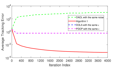
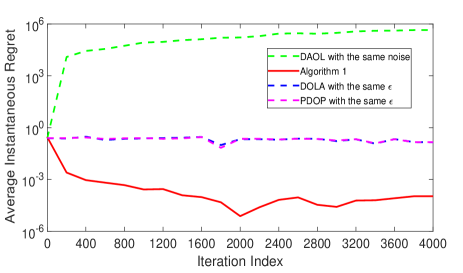
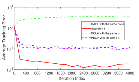
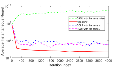
In this section, we use three numerical experiments to validate our theoretical results. In the first experiment, we consider the distributed online training of a logistic regression classifier using the “Mushrooms” and “Covtype” datasets [55]. In the second experiment, we consider distributed online training of a convolutional neural network (CNN) using the “MNIST” dataset [56]. In the third experiment, we train a CNN distributively using “CIFAR-10” dataset [57], which is a more diverse and challenging dataset than “MNIST”. In all three experiments, we compared Algorithm 1 with existing distributed autonomous online learning algorithm (DAOL) in [42] under the same DP-noise, and with existing DP approach for distributed online learning (DOLA) in [43] and the DP approach for distributed optimization (PDOP) in [29] under the condition that their privacy budget is equal to the maximum privacy budget (the weakest protection) among all learners in our algorithm. The interaction pattern in all experiments is the same, as depicted in Fig. 1.

Refer to caption
Figure 1: The interaction weights of five learners

VII-A Logistic regression using the “Mushrooms” and “Covtype” datasets

We first evaluated the effectiveness of Algorithm 1 by using an l2subscript𝑙2l_{2}-logistic regression classification problem on the “Mushrooms” and “Covtype” datasets [55]. In each iteration t𝑡t, we randomly sampled 555 data points for m=5𝑚5m=5 learners. All learners cooperatively track the optimal parameter θtsuperscriptsubscript𝜃𝑡\theta_{t}^{*} to the online optimization problem (2), in which the local loss function is given by

l(θ,ξti)=1Ntij=1Nti(1bti)(ati)Tθlog(s((ati)Tθ))+rti2θ2.𝑙𝜃superscriptsubscript𝜉𝑡𝑖1superscriptsubscript𝑁𝑡𝑖superscriptsubscript𝑗1superscriptsubscript𝑁𝑡𝑖1superscriptsubscript𝑏𝑡𝑖superscriptsuperscriptsubscript𝑎𝑡𝑖𝑇𝜃𝑠superscriptsuperscriptsubscript𝑎𝑡𝑖𝑇𝜃superscriptsubscript𝑟𝑡𝑖2superscriptnorm𝜃2l(\theta,\xi_{t}^{i})=\frac{1}{N_{t}^{i}}\sum_{j=1}^{N_{t}^{i}}(1-b_{t}^{i})(a_{t}^{i})^{T}\theta-\log(s((a_{t}^{i})^{T}\theta))+\frac{r_{t}^{i}}{2}\|\theta\|^{2}.

Here Ntisuperscriptsubscript𝑁𝑡𝑖N_{t}^{i} represents the number of data points per iteration, rti>0superscriptsubscript𝑟𝑡𝑖0r_{t}^{i}>0 is a regularization parameter proportional to 1Nti1superscriptsubscript𝑁𝑡𝑖\frac{1}{N_{t}^{i}}, and ξti=(ati,bti)𝒟isuperscriptsubscript𝜉𝑡𝑖superscriptsubscript𝑎𝑡𝑖superscriptsubscript𝑏𝑡𝑖subscript𝒟𝑖\xi_{t}^{i}=(a_{t}^{i},b_{t}^{i})\in\mathcal{D}_{i} represents the data point acquired by learner i𝑖i at time t𝑡t. s(a)=1/(1+ea)𝑠𝑎11superscript𝑒𝑎s(a)=1/(1+e^{-a}) is the sigmoid function.

In each iteration, we incorporated Laplace DP-noise with parameter νti=2(t+1)ςisuperscriptsubscript𝜈𝑡𝑖2superscript𝑡1superscript𝜍𝑖\nu_{t}^{i}=\sqrt{2}(t+1)^{\varsigma^{i}} to all shared messages, where ςi=0.1+0.02isuperscript𝜍𝑖0.10.02𝑖\varsigma^{i}=0.1+0.02i. Note that the multiplier i𝑖i in ςisuperscript𝜍𝑖\varsigma^{i} leads to different noise amplitudes and further different privacy budgets ϵisubscriptitalic-ϵ𝑖\epsilon_{i} for different learners. For the “Mushrooms” dataset, we configured the stepsize sequence and diminishing sequence as λt=1(t+1)0.8subscript𝜆𝑡1superscript𝑡10.8\lambda_{t}\!\!=\!\!\frac{1}{(t+1)^{0.8}} and γt=0.1(t+1)0.7subscript𝛾𝑡0.1superscript𝑡10.7\gamma_{t}\!\!=\!\!\frac{0.1}{(t+1)^{0.7}}, respectively. For the “Covtype” dataset, these values were set to λt=105(t+1)0.8subscript𝜆𝑡superscript105superscript𝑡10.8\lambda_{t}\!\!=\!\!\frac{10^{-5}}{(t+1)^{0.8}} and γt=0.1×10⁵(t+1)0.7subscript𝛾𝑡0.1superscript105superscript𝑡10.7\gamma_{t}\!\!=\!\!\frac{0.1\times 10^{-5}}{(t+1)^{0.7}}, respectively. Both configurations satisfy the conditions in Theorems 1-5. The algorithm was implemented for 4,00040004,000 iterations, during which the time-varying optimal parameter θtsuperscriptsubscript𝜃𝑡\theta_{t}^{*} was calculated using a noise-free, centralized gradient descent algorithm.

Refer to caption
(a) “Mushrooms”, Average tracking error
Refer to caption
(b) “Mushrooms”, Average instantaneous regret
Figure 2: Comparison of online logistic regression results by using the “Mushrooms” dataset.
Refer to caption
(a) “Covtype”, Average tracking error
Refer to caption
(b) “Covtype”, Average instantaneous regret
Figure 3: Comparison of online logistic regression results by using the “Covtype” dataset.

In the comparison, we selected the near-optimal stepsize sequences for DAOL, DOLA and PDOP such that doubling the stepsize results in nonconverging behavior. The resulting average tracking error and average instantaneous regret are shown in Fig. 2 and Fig. 3, respectively. It is clear that the proposed approach has a much better learning accuracy under the constraint of local differential privacy.

VII-B Neural network training using the “MNIST” dataset

In the second experiment, we assessed Algorithm 1’s performance through distributed online training of a convolutional neural network (CNN) using the “MNIST” dataset [56]. The training dataset was uniformly divided among learners. In each iteration, we randomly sampled 505050 images (mini-batch with size 505050) from the local dataset 𝒟isubscript𝒟𝑖\mathcal{D}_{i} and allocated them to learner i𝑖i for training. The training process spanned 666 epochs.

The CNN model for each learner consists of two convolutional layers (161616 and 323232 filters, respectively) followed by max pooling. The output is then flattened and directed through a 101010-unit fully connected layer for the 101010 classes (digits 00-999). In this experiment, we utilize Laplace DP-noise with parameter νti=2(t+1)ςisuperscriptsubscript𝜈𝑡𝑖2superscript𝑡1superscript𝜍𝑖\nu_{t}^{i}\!=\!\sqrt{2}(t+1)^{\varsigma^{i}} for all shared messages, where ςi=0.1+0.02isuperscript𝜍𝑖0.10.02𝑖\varsigma^{i}\!=\!0.1\!+\!0.02i. We set the stepsize sequence and decaying sequence to λt=1(t+1)0.71subscript𝜆𝑡1superscript𝑡10.71\lambda_{t}\!=\!\frac{1}{(t+1)^{0.71}} and γt=0.01(t+1)0.7subscript𝛾𝑡0.01superscript𝑡10.7\gamma_{t}\!=\!\frac{0.01}{(t+1)^{0.7}}, respectively.

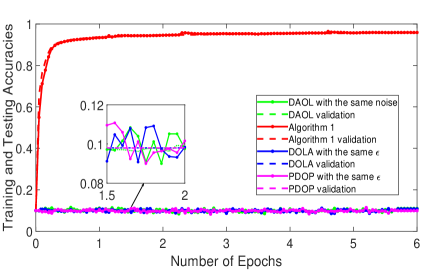
We compared our algorithm with the algorithm DAOL in [42] by training the same CNN, utilizing the same stepsize sequence and the same Laplace noise. Additionally, we implemented existing DP methods, DOLA in [43] and PDOP in [29], using the maximum privacy budget ϵ=maxi[m]{ϵi}italic-ϵsubscript𝑖delimited-[]𝑚subscriptitalic-ϵ𝑖\epsilon=\max_{i\in[m]}\{\epsilon_{i}\} in our algorithm, which corresponds to the weakest privacy protection among all nodes (i.e., incorporating DP-noise with decaying and homogeneous parameters νt=1104t+1subscript𝜈𝑡1superscript104𝑡1\nu_{t}\!=\!\frac{1}{10^{4}\sqrt{t+1}} and νt=(0.98)t104subscript𝜈𝑡superscript0.98𝑡superscript104\nu_{t}\!=\!\frac{(0.98)^{t}}{10^{4}} for DOLA and PDOP, respectively). The stepsize sequences for DOLA and PDOP followed their default parameters suggested in [43] and [29], respectively. Fig. 4 illustrates the training and testing accuracies.

The results reveal that under the given DP-noise, the DAOL algorithm falls short in training the CNN model. Besides, both the DOLA and PDOP algorithms are incapable of effectively training the CNN model. (Note that when the test data led to an exploding loss function — all happened when the training accuracy stalled around 0.10.10.1 in existing algorithms —, we used the initial parameter for validation, which always gave a testing accuracy of 0.10.10.1.) These results confirm the advantages of our proposed algorithm.

Refer to caption
Figure 4: Average training (solid lines) and testing (dash lines) accuracies for Algorithm 1 and existing algorithms DAOL, DOLA, and PDOP using the “MNIST” dataset.

VII-C Neural network training using the “CIFAR-10” dataset

In our third experiment, we appraised Algorithm 1’s performance via distributed online training of a CNN on the “CIFAR-10” dataset, which is one of the most widely used datasets for machine learning research (it is also more difficult to train than the “MNIST” dataset). The training dataset was evenly distributed among learners. During each iteration, we sequentially selected a mini-batch of 505050 images from the local dataset 𝒟isubscript𝒟𝑖\mathcal{D}_{i}, assigning them to learner i𝑖i for training. This training regimen was conducted over 1,00010001,000 epochs.

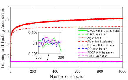
Each learner possesses a local copy of the CNN, which is composed of three convolutional layers (with 323232, 646464, and 128128128 filters, respectively), each succeeded by a max pooling layer. The output is then flattened and processed through two fully connected layers with 512512512 and 848484 neurons, respectively. The classification is conducted via a final, fully connected layer consisting of 101010 neurons representing the 101010 classes. In this experiment, all parameter designs are identical to those employed in the previous “MNIST” dataset experiment. The result in Fig. 5 once again confirms the effectiveness of our distributed online optimization algorithm for training the complex CNN model under the constraint of differential privacy.

Refer to caption
Figure 5: Average training (solid lines) and testing (dash lines) accuracies for Algorithm 1 and existing algorithms DAOL, DOLA, and PDOP using the “CIFAR-10” dataset.

VIII Conclusion

In this study, we have introduced a differentially private distributed online learning algorithm that successfully circumvents the trade-off between privacy and learning accuracy. More specifically, our proposed approach ensures a finite privacy budget on the infinite time horizon. This is in sharp contrast to existing DP methods for distributed online learning, which allow the privacy budget to grow to infinity, implying losing privacy protection when time tends to infinity. In addition, our approach also guarantees the convergence of expected instantaneous regret to zero. To the best of our knowledge, our approach is the first to achieve both rigorous local differential privacy and provable convergence in distributed online learning. Our numerical experiments on benchmark datasets confirm the advantages of the proposed approach over existing counterparts.

Appendix

VIII-A Proof of Lemma 1

Since θtsuperscriptsubscript𝜃𝑡\theta_{t}^{*} is the optimal solution to (2) and ΘΘ\Theta is a convex and compact set, the Euclidean projection property implies

Pro[θtc1Ft(θt)]=θt,c1>0,formulae-sequenceProdelimited-[]superscriptsubscript𝜃𝑡subscript𝑐1subscript𝐹𝑡superscriptsubscript𝜃𝑡superscriptsubscript𝜃𝑡for-allsubscript𝑐10\text{Pro}[\theta_{t}^{*}-c_{1}\nabla F_{t}(\theta_{t}^{*})]=\theta_{t}^{*},~{}\forall c_{1}>0,

which further leads to

θt+1θt2superscriptnormsuperscriptsubscript𝜃𝑡1superscriptsubscript𝜃𝑡2\displaystyle\|\theta_{t+1}^{*}-\theta_{t}^{*}\|^{2}
=Pro[θt+1c1Ft+1(θt+1)]Pro[θtc1Ft(θt)]2absentsuperscriptnormProdelimited-[]superscriptsubscript𝜃𝑡1subscript𝑐1subscript𝐹𝑡1superscriptsubscript𝜃𝑡1Prodelimited-[]superscriptsubscript𝜃𝑡subscript𝑐1subscript𝐹𝑡superscriptsubscript𝜃𝑡2\displaystyle=\|\text{Pro}[\theta_{t+1}^{*}-c_{1}\nabla F_{t+1}(\theta_{t+1}^{*})]-\text{Pro}[\theta_{t}^{*}-c_{1}\nabla F_{t}(\theta_{t}^{*})]\|^{2}
θt+1c1Ft+1(θt+1)θt+c1Ft(θt)2absentsuperscriptnormsuperscriptsubscript𝜃𝑡1subscript𝑐1subscript𝐹𝑡1superscriptsubscript𝜃𝑡1superscriptsubscript𝜃𝑡subscript𝑐1subscript𝐹𝑡superscriptsubscript𝜃𝑡2\displaystyle\leq\|\theta_{t+1}^{*}-c_{1}\nabla F_{t+1}(\theta_{t+1}^{*})-\theta_{t}^{*}+c_{1}\nabla F_{t}(\theta_{t}^{*})\|^{2}
2c1θt+1θt,Ft+1(θt+1)Ft(θt)absent2subscript𝑐1superscriptsubscript𝜃𝑡1superscriptsubscript𝜃𝑡subscript𝐹𝑡1superscriptsubscript𝜃𝑡1subscript𝐹𝑡superscriptsubscript𝜃𝑡\displaystyle\leq-2c_{1}\left\langle\theta_{t+1}^{*}-\theta_{t}^{*},\nabla F_{t+1}(\theta_{t+1}^{*})-\nabla F_{t}(\theta_{t}^{*})\right\rangle
+θt+1θt2+c12Ft+1(θt+1)Ft(θt)2.superscriptnormsuperscriptsubscript𝜃𝑡1superscriptsubscript𝜃𝑡2superscriptsubscript𝑐12superscriptnormsubscript𝐹𝑡1superscriptsubscript𝜃𝑡1subscript𝐹𝑡superscriptsubscript𝜃𝑡2\displaystyle\quad\quad+\|\theta_{t+1}^{*}\!-\!\theta_{t}^{*}\|^{2}+c_{1}^{2}\|\nabla F_{t+1}(\theta_{t+1}^{*})\!-\!\nabla F_{t}(\theta_{t}^{*})\|^{2}. (28)

Next, we estimate each term on the right hand side of (28):

2c1θt+1θt,Ft+1(θt+1)Ft(θt)2subscript𝑐1superscriptsubscript𝜃𝑡1superscriptsubscript𝜃𝑡subscript𝐹𝑡1superscriptsubscript𝜃𝑡1subscript𝐹𝑡superscriptsubscript𝜃𝑡\displaystyle 2c_{1}\left\langle\theta_{t+1}^{*}-\theta_{t}^{*},\nabla F_{t+1}(\theta_{t+1}^{*})-\nabla F_{t}(\theta_{t}^{*})\right\rangle (29)
=2c1θt+1θt,Ft+1(θt+1)Ft+1(θt)absent2subscript𝑐1superscriptsubscript𝜃𝑡1superscriptsubscript𝜃𝑡subscript𝐹𝑡1superscriptsubscript𝜃𝑡1subscript𝐹𝑡1superscriptsubscript𝜃𝑡\displaystyle=2c_{1}\left\langle\theta_{t+1}^{*}-\theta_{t}^{*},\nabla F_{t+1}(\theta_{t+1}^{*})-\nabla F_{t+1}(\theta_{t}^{*})\right\rangle
+2c1θt+1θt,Ft+1(θt)Ft(θt).2subscript𝑐1superscriptsubscript𝜃𝑡1superscriptsubscript𝜃𝑡subscript𝐹𝑡1superscriptsubscript𝜃𝑡subscript𝐹𝑡superscriptsubscript𝜃𝑡\displaystyle\quad\quad+2c_{1}\left\langle\theta_{t+1}^{*}-\theta_{t}^{*},\nabla F_{t+1}(\theta_{t}^{*})-\nabla F_{t}(\theta_{t}^{*})\right\rangle.

By using the Young’s inequality, we have the following relationship for the second term on the right hand side of (29):

|θt+1θt,Ft+1(θt)Ft(θt)|superscriptsubscript𝜃𝑡1superscriptsubscript𝜃𝑡subscript𝐹𝑡1superscriptsubscript𝜃𝑡subscript𝐹𝑡superscriptsubscript𝜃𝑡\displaystyle\left|\left\langle\theta_{t+1}^{*}-\theta_{t}^{*},\nabla F_{t+1}(\theta_{t}^{*})-\nabla F_{t}(\theta_{t}^{*})\right\rangle\right|
μ4θt+1θt2+1μFt+1(θt)Ft(θt)2.absent𝜇4superscriptnormsuperscriptsubscript𝜃𝑡1superscriptsubscript𝜃𝑡21𝜇superscriptnormsubscript𝐹𝑡1superscriptsubscript𝜃𝑡subscript𝐹𝑡superscriptsubscript𝜃𝑡2\displaystyle\leq\frac{\mu}{4}\|\theta_{t+1}^{*}-\theta_{t}^{*}\|^{2}+\frac{1}{\mu}\|\nabla F_{t+1}(\theta_{t}^{*})-\nabla F_{t}(\theta_{t}^{*})\|^{2}. (30)

The last term on the right hand side of (30) satisfies

Ft+1(θt)Ft(θt)subscript𝐹𝑡1superscriptsubscript𝜃𝑡subscript𝐹𝑡superscriptsubscript𝜃𝑡\displaystyle\nabla F_{t+1}(\theta_{t}^{*})-\nabla F_{t}(\theta_{t}^{*}) (31)
=1mi=1m(1t+2k=0t+1l(θt,ξki)1(t+1)k=0tl(θt,ξki))absent1𝑚superscriptsubscript𝑖1𝑚1𝑡2superscriptsubscript𝑘0𝑡1𝑙superscriptsubscript𝜃𝑡superscriptsubscript𝜉𝑘𝑖1𝑡1superscriptsubscript𝑘0𝑡𝑙superscriptsubscript𝜃𝑡superscriptsubscript𝜉𝑘𝑖\displaystyle=\frac{1}{m}\sum_{i=1}^{m}\!\left(\!\frac{1}{t+2}\sum_{k=0}^{t+1}\nabla l(\theta_{t}^{*},\xi_{k}^{i})\!-\!\frac{1}{(t\!+\!1)}\sum_{k=0}^{t}\nabla l(\theta_{t}^{*},\xi_{k}^{i})\!\right)
=1mi=1m(1t+2l(θt,ξt+1i)1(t+1)(t+2)k=0tl(θt,ξki))absent1𝑚superscriptsubscript𝑖1𝑚1𝑡2𝑙superscriptsubscript𝜃𝑡superscriptsubscript𝜉𝑡1𝑖1𝑡1𝑡2superscriptsubscript𝑘0𝑡𝑙superscriptsubscript𝜃𝑡superscriptsubscript𝜉𝑘𝑖\displaystyle=\frac{1}{m}\sum_{i=1}^{m}\!\left(\!\frac{1}{t+2}\nabla l(\theta_{t}^{*},\xi_{t+1}^{i})\!-\!\frac{1}{(t\!+\!1)(t\!+\!2)}\sum_{k=0}^{t}\nabla l(\theta_{t}^{*},\xi_{k}^{i})\!\right)
1mi=1m(2l(θt,ξt+1i)t+22+2k=0tl(θt,ξki)(t+1)(t+2)2).absent1𝑚superscriptsubscript𝑖1𝑚2superscriptnorm𝑙superscriptsubscript𝜃𝑡superscriptsubscript𝜉𝑡1𝑖𝑡222superscriptnormsuperscriptsubscript𝑘0𝑡𝑙superscriptsubscript𝜃𝑡superscriptsubscript𝜉𝑘𝑖𝑡1𝑡22\displaystyle\leq\frac{1}{m}\sum_{i=1}^{m}\left(2\left\|\frac{\nabla l(\theta_{t}^{*},\xi_{t+1}^{i})}{t+2}\right\|^{2}+2\left\|\frac{\sum_{k=0}^{t}\nabla l(\theta_{t}^{*},\xi_{k}^{i})}{(t+1)(t+2)}\right\|^{2}\right).

By using Assumption 1(iii) and Assumption 3(ii), we have 𝔼[l(θt,ξti)2|t]2(κ2+D2)𝔼delimited-[]conditionalsuperscriptnorm𝑙superscriptsubscript𝜃𝑡superscriptsubscript𝜉𝑡𝑖2subscript𝑡2superscript𝜅2superscript𝐷2\mathbb{E}\left[\|\nabla l(\theta_{t}^{*},\xi_{t}^{i})\|^{2}\Big{|}\mathcal{F}_{t}\right]\!\leq\!2(\kappa^{2}\!+\!D^{2}). By taking the conditional expectation on both sides of (31), one obtains

𝔼[Ft+1(θt)Ft(θt)2|t]8(κ2+D2)(t+1)2.𝔼delimited-[]conditionalsuperscriptnormsubscript𝐹𝑡1superscriptsubscript𝜃𝑡subscript𝐹𝑡superscriptsubscript𝜃𝑡2subscript𝑡8superscript𝜅2superscript𝐷2superscript𝑡12\mathbb{E}\left[\|\nabla F_{t+1}(\theta_{t}^{*})-\nabla F_{t}(\theta_{t}^{*})\|^{2}\Big{|}\mathcal{F}_{t}\right]\leq\frac{8(\kappa^{2}+D^{2})}{(t+1)^{2}}. (32)

Substituting (32) into (30) yields

2c1𝔼[θt+1θt,Ft+1(θt)Ft(θt)|t]2subscript𝑐1𝔼delimited-[]conditionalsuperscriptsubscript𝜃𝑡1superscriptsubscript𝜃𝑡subscript𝐹𝑡1superscriptsubscript𝜃𝑡subscript𝐹𝑡superscriptsubscript𝜃𝑡subscript𝑡\displaystyle 2c_{1}\mathbb{E}\left[\left\langle\theta_{t+1}^{*}-\theta_{t}^{*},\nabla F_{t+1}(\theta_{t}^{*})-\nabla F_{t}(\theta_{t}^{*})\right\rangle\Big{|}\mathcal{F}_{t}\right] (33)
2c1(μ4θt+1θt2+8(κ2+D2)μ(t+1)2).absent2subscript𝑐1𝜇4superscriptnormsuperscriptsubscript𝜃𝑡1superscriptsubscript𝜃𝑡28superscript𝜅2superscript𝐷2𝜇superscript𝑡12\displaystyle\geq-2c_{1}\left(\frac{\mu}{4}\|\theta_{t+1}^{*}-\theta_{t}^{*}\|^{2}+\frac{8(\kappa^{2}+D^{2})}{\mu(t+1)^{2}}\right).

Assumption 1(ii) with μ>0𝜇0\mu>0 implies

2c1𝔼[θt+1θt,Ft+1(θt+1)Ft(θt)|t]2subscript𝑐1𝔼delimited-[]conditionalsuperscriptsubscript𝜃𝑡1superscriptsubscript𝜃𝑡subscript𝐹𝑡1superscriptsubscript𝜃𝑡1subscript𝐹𝑡superscriptsubscript𝜃𝑡subscript𝑡\displaystyle 2c_{1}\mathbb{E}\left[\langle\theta_{t+1}^{*}-\theta_{t}^{*},\nabla F_{t+1}(\theta_{t+1}^{*})-\nabla F_{t}(\theta_{t}^{*})\rangle\Big{|}\mathcal{F}_{t}\right]
2c1μθt+1θt2.absent2subscript𝑐1𝜇superscriptnormsuperscriptsubscript𝜃𝑡1superscriptsubscript𝜃𝑡2\displaystyle\geq 2c_{1}\mu\|\theta_{t+1}^{*}-\theta_{t}^{*}\|^{2}. (34)

Plugging (33) and (34) into (29) leads to

2c1𝔼[θt+1θt,Ft+1(θt+1)Ft(θt)|t]2subscript𝑐1𝔼delimited-[]conditionalsuperscriptsubscript𝜃𝑡1superscriptsubscript𝜃𝑡subscript𝐹𝑡1superscriptsubscript𝜃𝑡1subscript𝐹𝑡superscriptsubscript𝜃𝑡subscript𝑡\displaystyle 2c_{1}\mathbb{E}\left[\left\langle\theta_{t+1}^{*}-\theta_{t}^{*},\nabla F_{t+1}(\theta_{t+1}^{*})-\nabla F_{t}(\theta_{t}^{*})\right\rangle\Big{|}\mathcal{F}_{t}\right] (35)
3c1μ2θt+1θt216c1(κ2+D2)μ(t+1)2.absent3subscript𝑐1𝜇2superscriptnormsuperscriptsubscript𝜃𝑡1superscriptsubscript𝜃𝑡216subscript𝑐1superscript𝜅2superscript𝐷2𝜇superscript𝑡12\displaystyle\geq\frac{3c_{1}\mu}{2}\|\theta_{t+1}^{*}-\theta_{t}^{*}\|^{2}-\frac{16c_{1}(\kappa^{2}+D^{2})}{\mu(t+1)^{2}}.

The Lipschitz property in Assumption 3(iii) and (32) imply

c12𝔼[Ft+1(θt+1)Ft(θt)2|t]superscriptsubscript𝑐12𝔼delimited-[]conditionalsuperscriptnormsubscript𝐹𝑡1superscriptsubscript𝜃𝑡1subscript𝐹𝑡superscriptsubscript𝜃𝑡2subscript𝑡\displaystyle c_{1}^{2}\mathbb{E}\left[\|\nabla F_{t+1}(\theta_{t+1}^{*})-\nabla F_{t}(\theta_{t}^{*})\|^{2}\Big{|}\mathcal{F}_{t}\right] (36)
2c12L2θt+1θt2+16c12(κ2+D2)(t+1)2.absent2superscriptsubscript𝑐12superscript𝐿2superscriptnormsuperscriptsubscript𝜃𝑡1superscriptsubscript𝜃𝑡216superscriptsubscript𝑐12superscript𝜅2superscript𝐷2superscript𝑡12\displaystyle\leq 2c_{1}^{2}L^{2}\|\theta_{t+1}^{*}-\theta_{t}^{*}\|^{2}+\frac{16c_{1}^{2}(\kappa^{2}+D^{2})}{(t+1)^{2}}.

Plugging (35) and (36) into (28) leads to

𝔼[θt+1θt2|t]𝔼delimited-[]conditionalsuperscriptnormsuperscriptsubscript𝜃𝑡1superscriptsubscript𝜃𝑡2subscript𝑡\displaystyle\mathbb{E}\left[\|\theta_{t+1}^{*}-\theta_{t}^{*}\|^{2}\Big{|}\mathcal{F}_{t}\right]
θt+1θt2(3c1μ22c12L2)θt+1θt2absentsuperscriptnormsuperscriptsubscript𝜃𝑡1superscriptsubscript𝜃𝑡23subscript𝑐1𝜇22superscriptsubscript𝑐12superscript𝐿2superscriptnormsuperscriptsubscript𝜃𝑡1superscriptsubscript𝜃𝑡2\displaystyle\leq\|\theta_{t+1}^{*}-\theta_{t}^{*}\|^{2}-\left(\frac{3c_{1}\mu}{2}-2c_{1}^{2}L^{2}\right)\|\theta_{t+1}^{*}-\theta_{t}^{*}\|^{2}
+(1μ+c1)16c1(κ2+D2)(t+1)2.1𝜇subscript𝑐116subscript𝑐1superscript𝜅2superscript𝐷2superscript𝑡12\displaystyle\quad\quad+\left(\frac{1}{\mu}+c_{1}\right)\frac{16c_{1}(\kappa^{2}+D^{2})}{(t+1)^{2}}.

We choose c1=μ2L2subscript𝑐1𝜇2superscript𝐿2c_{1}=\frac{\mu}{2L^{2}} (i.e., c1μ=2c12L2subscript𝑐1𝜇2superscriptsubscript𝑐12superscript𝐿2c_{1}\mu=2c_{1}^{2}L^{2}) to obtain

c1μ2𝔼[θt+1θt2|t](1μ+c1)16c1(κ2+D2)(t+1)2,subscript𝑐1𝜇2𝔼delimited-[]conditionalsuperscriptnormsuperscriptsubscript𝜃𝑡1superscriptsubscript𝜃𝑡2subscript𝑡1𝜇subscript𝑐116subscript𝑐1superscript𝜅2superscript𝐷2superscript𝑡12\displaystyle\frac{c_{1}\mu}{2}\mathbb{E}\left[\|\theta_{t+1}^{*}-\theta_{t}^{*}\|^{2}\Big{|}\mathcal{F}_{t}\right]\leq\left(\frac{1}{\mu}+c_{1}\right)\frac{16c_{1}(\kappa^{2}+D^{2})}{(t+1)^{2}},

which further implies inequality (11) in Lemma 1.

VIII-B Proof of Theorem 1

For the sake of notational simplicity, we denote 𝜽~t=𝜽t𝜽tsubscriptbold-~𝜽𝑡subscript𝜽𝑡superscriptsubscript𝜽𝑡\boldsymbol{\tilde{\theta}}_{t}=\boldsymbol{\theta}_{t}-\boldsymbol{\theta}_{t}^{*}, θ¯t=1mi=1mθtisubscript¯𝜃𝑡1𝑚superscriptsubscript𝑖1𝑚superscriptsubscript𝜃𝑡𝑖\bar{\theta}_{t}=\frac{1}{m}\sum_{i=1}^{m}\theta_{t}^{i}, 𝜽¯t=𝟏mθ¯tsubscriptbold-¯𝜽𝑡tensor-productsubscript1𝑚subscript¯𝜃𝑡\boldsymbol{\bar{\theta}}_{t}=\boldsymbol{1}_{m}\otimes\bar{\theta}_{t}, 𝜽ˇt=𝜽t𝜽¯tsubscriptbold-ˇ𝜽𝑡subscript𝜽𝑡subscript¯𝜽𝑡\boldsymbol{\check{\theta}}_{t}=\boldsymbol{\theta}_{t}-\bar{\boldsymbol{\theta}}_{t}, 𝒅t(𝜽t)=col(dt1(θt1),,dtm(θtm))subscript𝒅𝑡subscript𝜽𝑡colsuperscriptsubscript𝑑𝑡1superscriptsubscript𝜃𝑡1superscriptsubscript𝑑𝑡𝑚superscriptsubscript𝜃𝑡𝑚\boldsymbol{d}_{t}(\boldsymbol{\theta}_{t})=\text{col}(d_{t}^{1}(\theta_{t}^{1}),\cdots,d_{t}^{m}(\theta_{t}^{m})), ζtwi=j𝒩iwijζtjsuperscriptsubscript𝜁𝑡𝑤𝑖subscript𝑗subscript𝒩𝑖subscript𝑤𝑖𝑗superscriptsubscript𝜁𝑡𝑗\zeta_{t}^{wi}=\sum_{j\in{\mathcal{N}_{i}}}w_{ij}\zeta_{t}^{j}, 𝜻tw=col(ζtw1,,ζtwm)superscriptsubscript𝜻𝑡𝑤colsuperscriptsubscript𝜁𝑡𝑤1superscriptsubscript𝜁𝑡𝑤𝑚\boldsymbol{\zeta}_{t}^{w}=\text{col}(\zeta_{t}^{w1},\cdots,\zeta_{t}^{wm}), and 𝝈t=col(σt1,,σtm)subscript𝝈𝑡colsuperscriptsubscript𝜎𝑡1superscriptsubscript𝜎𝑡𝑚\boldsymbol{\sigma}_{t}=\text{col}(\sigma_{t}^{1},\cdots,\sigma_{t}^{m}).

Lemma 4.

Under the conditions in Theorem 1, the following inequality always holds:

𝔼[𝜽t+1𝜽t+12|t]𝔼delimited-[]conditionalsuperscriptnormsubscript𝜽𝑡1superscriptsubscript𝜽𝑡12subscript𝑡\displaystyle\mathbb{E}\left[\|\boldsymbol{\theta}_{t+1}-\boldsymbol{\boldsymbol{\theta}}_{t+1}^{*}\|^{2}\Big{|}\mathcal{F}_{t}\right]
at(𝜽~t2+2γt𝜽~tT(WIn)𝜽~t2mλt(Ft(θ¯t)Ft(θt))\displaystyle\leq a_{t}\Big{(}\|\boldsymbol{\tilde{\theta}}_{t}\|^{2}+2\gamma_{t}\boldsymbol{\tilde{\theta}}_{t}^{T}(W\otimes I_{n})\boldsymbol{\tilde{\theta}}_{t}-2m\lambda_{t}(F_{t}(\bar{\theta}_{t})-F_{t}(\theta_{t}^{*}))
3μλt8𝜽~t2+λt(μ+8L2μ)𝜽ˇt2+3γt2(WIn)𝜽~t23𝜇subscript𝜆𝑡8superscriptnormsubscriptbold-~𝜽𝑡2subscript𝜆𝑡𝜇8superscript𝐿2𝜇superscriptnormsubscriptbold-ˇ𝜽𝑡23superscriptsubscript𝛾𝑡2superscriptnormtensor-product𝑊subscript𝐼𝑛subscriptbold-~𝜽𝑡2\displaystyle\quad-\frac{3\mu\lambda_{t}}{8}\|\boldsymbol{\tilde{\theta}}_{t}\|^{2}+\lambda_{t}(\mu+\frac{8L^{2}}{\mu})\|\boldsymbol{\check{\theta}}_{t}\|^{2}+3\gamma_{t}^{2}\|(W\otimes I_{n})\boldsymbol{\tilde{\theta}}_{t}\|^{2}
+3γt2𝝈t2+3λt2𝒅t(𝜽t)2)+bt𝜽t+1𝜽t2,\displaystyle\quad+3\gamma_{t}^{2}\|\boldsymbol{\sigma}_{t}\|^{2}+3\lambda_{t}^{2}\|\boldsymbol{d}_{t}(\boldsymbol{\theta}_{t})\|^{2}\Big{)}+b_{t}\|\boldsymbol{\theta}_{t+1}^{*}-\boldsymbol{\theta}_{t}^{*}\|^{2}, (37)

where nonnegative sequences atsubscript𝑎𝑡a_{t} and btsubscript𝑏𝑡b_{t} are given by at=1+3μλt16subscript𝑎𝑡13𝜇subscript𝜆𝑡16a_{t}=1+\frac{3\mu\lambda_{t}}{16} and bt=1+163λtμsubscript𝑏𝑡1163subscript𝜆𝑡𝜇b_{t}=1+\frac{16}{3\lambda_{t}\mu}, respectively.

Proof.

The dynamic (6) in Algorithm 1 can be written into the following compact form:

𝜽^t+1=(I+γt(WIn))𝜽t+γt𝜻twλt𝒅t(𝜽t).subscriptbold-^𝜽𝑡1𝐼subscript𝛾𝑡tensor-product𝑊subscript𝐼𝑛subscript𝜽𝑡subscript𝛾𝑡superscriptsubscript𝜻𝑡𝑤subscript𝜆𝑡subscript𝒅𝑡subscript𝜽𝑡\boldsymbol{\hat{\theta}}_{t+1}=(I+\gamma_{t}(W\otimes I_{n}))\boldsymbol{\theta}_{t}+\gamma_{t}\boldsymbol{\zeta}_{t}^{w}-\lambda_{t}\boldsymbol{d}_{t}(\boldsymbol{\theta}_{t}).

By using the projection inequality, we obtain

𝜽t+1𝜽t2=Pro[𝜽^t+1]𝜽t2𝜽^t+1𝜽t2superscriptnormsubscript𝜽𝑡1superscriptsubscript𝜽𝑡2superscriptnormProdelimited-[]subscriptbold-^𝜽𝑡1superscriptsubscript𝜽𝑡2superscriptnormsubscriptbold-^𝜽𝑡1superscriptsubscript𝜽𝑡2\displaystyle\|\boldsymbol{\theta}_{t+1}-\boldsymbol{\boldsymbol{\theta}}_{t}^{*}\|^{2}=\|\text{Pro}[\boldsymbol{\hat{\theta}}_{t+1}]-\boldsymbol{\theta}_{t}^{*}\|^{2}\leq\|\boldsymbol{\hat{\theta}}_{t+1}-\boldsymbol{\theta}_{t}^{*}\|^{2} (38)
𝜽~t2+γt(WIn)𝜽t+γt𝜻twλt𝒅t(𝜽t)2absentsuperscriptnormsubscriptbold-~𝜽𝑡2superscriptnormsubscript𝛾𝑡tensor-product𝑊subscript𝐼𝑛subscript𝜽𝑡subscript𝛾𝑡superscriptsubscript𝜻𝑡𝑤subscript𝜆𝑡subscript𝒅𝑡subscript𝜽𝑡2\displaystyle\leq\|\boldsymbol{\tilde{\theta}}_{t}\|^{2}+\|\gamma_{t}(W\otimes I_{n})\boldsymbol{\theta}_{t}+\gamma_{t}\boldsymbol{\zeta}_{t}^{w}-\lambda_{t}\boldsymbol{d}_{t}(\boldsymbol{\theta}_{t})\|^{2}
+2𝜽~t,γt(WIn)𝜽t+γt𝜻twλt𝒅t(𝜽t).2subscriptbold-~𝜽𝑡subscript𝛾𝑡tensor-product𝑊subscript𝐼𝑛subscript𝜽𝑡subscript𝛾𝑡superscriptsubscript𝜻𝑡𝑤subscript𝜆𝑡subscript𝒅𝑡subscript𝜽𝑡\displaystyle\quad\quad+2\left\langle\boldsymbol{\tilde{\theta}}_{t},\gamma_{t}(W\otimes I_{n})\boldsymbol{\theta}_{t}+\gamma_{t}\boldsymbol{\zeta}_{t}^{w}-\lambda_{t}\boldsymbol{d}_{t}(\boldsymbol{\theta}_{t})\right\rangle.

Recalling W𝟏=𝟎𝑊10W\mathbf{1}=\mathbf{0}, inequality (38) can be rewritten as

𝜽t+1𝜽t2superscriptnormsubscript𝜽𝑡1superscriptsubscript𝜽𝑡2\displaystyle\|\boldsymbol{\theta}_{t+1}-\boldsymbol{\boldsymbol{\theta}}_{t}^{*}\|^{2} (39)
γt(WIn)𝜽~t+γt𝜻twλt𝒅t(𝜽t)2absentsuperscriptnormsubscript𝛾𝑡tensor-product𝑊subscript𝐼𝑛subscriptbold-~𝜽𝑡subscript𝛾𝑡superscriptsubscript𝜻𝑡𝑤subscript𝜆𝑡subscript𝒅𝑡subscript𝜽𝑡2\displaystyle\leq\|\gamma_{t}(W\otimes I_{n})\boldsymbol{\tilde{\theta}}_{t}+\gamma_{t}\boldsymbol{\zeta}_{t}^{w}-\lambda_{t}\boldsymbol{d}_{t}(\boldsymbol{\theta}_{t})\|^{2}
+𝜽~t2+2𝜽~t,γt(WIn)𝜽~t+γt𝜻twλt𝒅t(𝜽t).superscriptnormsubscriptbold-~𝜽𝑡22subscriptbold-~𝜽𝑡subscript𝛾𝑡tensor-product𝑊subscript𝐼𝑛subscriptbold-~𝜽𝑡subscript𝛾𝑡superscriptsubscript𝜻𝑡𝑤subscript𝜆𝑡subscript𝒅𝑡subscript𝜽𝑡\displaystyle\quad\quad+\|\boldsymbol{\tilde{\theta}}_{t}\|^{2}+2\left\langle\boldsymbol{\tilde{\theta}}_{t},\gamma_{t}(W\otimes I_{n})\boldsymbol{\tilde{\theta}}_{t}+\gamma_{t}\boldsymbol{\zeta}_{t}^{w}-\lambda_{t}\boldsymbol{d}_{t}(\boldsymbol{\theta}_{t})\right\rangle.

By using Assumption 4, we have

𝔼[𝜽~t,γt(WIn)𝜽~t+γt𝜻twλt𝒅t(𝜽t)|t]𝔼delimited-[]conditionalsubscriptbold-~𝜽𝑡subscript𝛾𝑡tensor-product𝑊subscript𝐼𝑛subscriptbold-~𝜽𝑡subscript𝛾𝑡superscriptsubscript𝜻𝑡𝑤subscript𝜆𝑡subscript𝒅𝑡subscript𝜽𝑡subscript𝑡\displaystyle\mathbb{E}\left[\left\langle\boldsymbol{\tilde{\theta}}_{t},\gamma_{t}(W\otimes I_{n})\boldsymbol{\tilde{\theta}}_{t}+\gamma_{t}\boldsymbol{\zeta}_{t}^{w}-\lambda_{t}\boldsymbol{d}_{t}(\boldsymbol{\theta}_{t})\right\rangle\Big{|}\mathcal{F}_{t}\right] (40)
=γt𝜽~tT(WIn)𝜽~t𝜽~t,λt𝒅t(𝜽t).absentsubscript𝛾𝑡superscriptsubscriptbold-~𝜽𝑡𝑇tensor-product𝑊subscript𝐼𝑛subscriptbold-~𝜽𝑡subscriptbold-~𝜽𝑡subscript𝜆𝑡subscript𝒅𝑡subscript𝜽𝑡\displaystyle=\gamma_{t}\boldsymbol{\tilde{\theta}}_{t}^{T}(W\otimes I_{n})\boldsymbol{\tilde{\theta}}_{t}-\left\langle\boldsymbol{\tilde{\theta}}_{t},\lambda_{t}\boldsymbol{d}_{t}(\boldsymbol{\theta}_{t})\right\rangle.

We use the Cauchy-Schwartz inequality to obtain

γt(WIn)𝜽~t+γt𝜻twλt𝒅t(𝜽t)2superscriptnormsubscript𝛾𝑡tensor-product𝑊subscript𝐼𝑛subscriptbold-~𝜽𝑡subscript𝛾𝑡superscriptsubscript𝜻𝑡𝑤subscript𝜆𝑡subscript𝒅𝑡subscript𝜽𝑡2\displaystyle\|\gamma_{t}(W\otimes I_{n})\boldsymbol{\tilde{\theta}}_{t}+\gamma_{t}\boldsymbol{\zeta}_{t}^{w}-\lambda_{t}\boldsymbol{d}_{t}(\boldsymbol{\theta}_{t})\|^{2} (41)
3γt2(WIn)𝜽~t2+3γt2𝝈t2+3λt2𝒅t(𝜽t)2.absent3superscriptsubscript𝛾𝑡2superscriptnormtensor-product𝑊subscript𝐼𝑛subscriptbold-~𝜽𝑡23superscriptsubscript𝛾𝑡2superscriptnormsubscript𝝈𝑡23superscriptsubscript𝜆𝑡2superscriptnormsubscript𝒅𝑡subscript𝜽𝑡2\displaystyle\leq 3\gamma_{t}^{2}\|(W\otimes I_{n})\boldsymbol{\tilde{\theta}}_{t}\|^{2}+3\gamma_{t}^{2}\|\boldsymbol{\sigma}_{t}\|^{2}+3\lambda_{t}^{2}\|\boldsymbol{d}_{t}(\boldsymbol{\theta}_{t})\|^{2}.

Substituting (40) and (41) into (39) leads to

𝔼[𝜽t+1𝜽t2|t]𝔼delimited-[]conditionalsuperscriptnormsubscript𝜽𝑡1superscriptsubscript𝜽𝑡2subscript𝑡\displaystyle\mathbb{E}\left[\|\boldsymbol{\theta}_{t+1}-\boldsymbol{\boldsymbol{\theta}}_{t}^{*}\|^{2}\Big{|}\mathcal{F}_{t}\right] (42)
𝜽~t2+2γt𝜽~tT(WIn)𝜽~t2λt𝜽~t,𝒅t(𝜽t)absentsuperscriptnormsubscriptbold-~𝜽𝑡22subscript𝛾𝑡superscriptsubscriptbold-~𝜽𝑡𝑇tensor-product𝑊subscript𝐼𝑛subscriptbold-~𝜽𝑡2subscript𝜆𝑡subscriptbold-~𝜽𝑡subscript𝒅𝑡subscript𝜽𝑡\displaystyle\leq\|\boldsymbol{\tilde{\theta}}_{t}\|^{2}+2\gamma_{t}\boldsymbol{\tilde{\theta}}_{t}^{T}(W\otimes I_{n})\boldsymbol{\tilde{\theta}}_{t}-2\lambda_{t}\left\langle\boldsymbol{\tilde{\theta}}_{t},\boldsymbol{d}_{t}(\boldsymbol{\theta}_{t})\right\rangle
+3γt2(WIn)𝜽~t2+3γt2𝝈t2+3λt2𝒅t(𝜽t)2.3superscriptsubscript𝛾𝑡2superscriptnormtensor-product𝑊subscript𝐼𝑛subscriptbold-~𝜽𝑡23superscriptsubscript𝛾𝑡2superscriptnormsubscript𝝈𝑡23superscriptsubscript𝜆𝑡2superscriptnormsubscript𝒅𝑡subscript𝜽𝑡2\displaystyle\quad+3\gamma_{t}^{2}\|(W\otimes I_{n})\boldsymbol{\tilde{\theta}}_{t}\|^{2}\!+\!3\gamma_{t}^{2}\|\boldsymbol{\sigma}_{t}\|^{2}\!+\!3\lambda_{t}^{2}\|\boldsymbol{d}_{t}(\boldsymbol{\theta}_{t})\|^{2}.

The third term on the right hand side of (42) can be decomposed into

2λt𝔼[𝜽~t,𝒅t(𝜽t)|t]2subscript𝜆𝑡𝔼delimited-[]conditionalsubscriptbold-~𝜽𝑡subscript𝒅𝑡subscript𝜽𝑡subscript𝑡\displaystyle 2\lambda_{t}\mathbb{E}\left[\left\langle\boldsymbol{\tilde{\theta}}_{t},\boldsymbol{d}_{t}(\boldsymbol{\theta}_{t})\right\rangle\Big{|}\mathcal{F}_{t}\right] (43)
=2λt𝜽~t,𝒅t(𝜽¯t)+2λt𝜽~t,𝒅t(𝜽t)𝒅t(𝜽¯t).absent2subscript𝜆𝑡subscriptbold-~𝜽𝑡subscript𝒅𝑡subscriptbold-¯𝜽𝑡2subscript𝜆𝑡subscriptbold-~𝜽𝑡subscript𝒅𝑡subscript𝜽𝑡subscript𝒅𝑡subscriptbold-¯𝜽𝑡\displaystyle=2\lambda_{t}\left\langle\boldsymbol{\tilde{\theta}}_{t},\boldsymbol{d}_{t}(\boldsymbol{\bar{\theta}}_{t})\right\rangle+\!2\lambda_{t}\left\langle\boldsymbol{\tilde{\theta}}_{t},\boldsymbol{d}_{t}(\boldsymbol{\theta}_{t})\!-\!\boldsymbol{d}_{t}(\boldsymbol{\bar{\theta}}_{t})\right\rangle.

By using Assumption 1(ii), Assumption 3(i), and the relation i=1mθti=mθ¯tsuperscriptsubscript𝑖1𝑚superscriptsubscript𝜃𝑡𝑖𝑚subscript¯𝜃𝑡\sum_{i=1}^{m}\theta_{t}^{i}=m\bar{\theta}_{t}, we have

𝔼[2λt𝜽~t,𝒅t(𝜽¯t)|t]𝔼delimited-[]conditional2subscript𝜆𝑡subscriptbold-~𝜽𝑡subscript𝒅𝑡subscriptbold-¯𝜽𝑡subscript𝑡\displaystyle\mathbb{E}\left[2\lambda_{t}\left\langle\boldsymbol{\tilde{\theta}}_{t},\boldsymbol{d}_{t}(\boldsymbol{\bar{\theta}}_{t})\right\rangle\Big{|}\mathcal{F}_{t}\right] (44)
2λti=1m(fi(θ¯t)fi(θt)+μ2θ¯tθt2)absent2subscript𝜆𝑡superscriptsubscript𝑖1𝑚subscript𝑓𝑖subscript¯𝜃𝑡subscript𝑓𝑖superscriptsubscript𝜃𝑡𝜇2superscriptnormsubscript¯𝜃𝑡superscriptsubscript𝜃𝑡2\displaystyle\geq 2\lambda_{t}\sum_{i=1}^{m}\left(f_{i}(\bar{\theta}_{t})-f_{i}(\theta_{t}^{*})+\frac{\mu}{2}\|\bar{\theta}_{t}-\theta_{t}^{*}\|^{2}\right)
2λt(mFt(θ¯t)mFt(θt)+μ4𝜽~t2μ2𝜽ˇt2).absent2subscript𝜆𝑡𝑚subscript𝐹𝑡subscript¯𝜃𝑡𝑚subscript𝐹𝑡superscriptsubscript𝜃𝑡𝜇4superscriptnormsubscriptbold-~𝜽𝑡2𝜇2superscriptnormsubscriptbold-ˇ𝜽𝑡2\displaystyle\geq 2\lambda_{t}\left(mF_{t}(\bar{\theta}_{t})-mF_{t}(\theta_{t}^{*})+\frac{\mu}{4}\|\boldsymbol{\tilde{\theta}}_{t}\|^{2}-\frac{\mu}{2}\|\boldsymbol{\check{\theta}}_{t}\|^{2}\right).

The Lipschitz property in Assumption 3(iii) implies

𝔼[2λt𝜽~t,𝒅t(𝜽t)𝒅t(𝜽¯t)|t]𝔼delimited-[]conditional2subscript𝜆𝑡subscriptbold-~𝜽𝑡subscript𝒅𝑡subscript𝜽𝑡subscript𝒅𝑡subscriptbold-¯𝜽𝑡subscript𝑡\displaystyle\mathbb{E}\left[2\lambda_{t}\left\langle\boldsymbol{\tilde{\theta}}_{t},\boldsymbol{d}_{t}(\boldsymbol{\theta}_{t})\!-\!\boldsymbol{d}_{t}(\boldsymbol{\bar{\theta}}_{t})\right\rangle\Big{|}\mathcal{F}_{t}\right]
2λt(μ16𝜽~t2+16μ𝒅t(𝜽t)𝒅t(𝜽¯t)2)absent2subscript𝜆𝑡𝜇16superscriptnormsubscriptbold-~𝜽𝑡216𝜇superscriptnormsubscript𝒅𝑡subscript𝜽𝑡subscript𝒅𝑡subscriptbold-¯𝜽𝑡2\displaystyle\geq-2\lambda_{t}\left(\frac{\mu}{16}\|\boldsymbol{\tilde{\theta}}_{t}\|^{2}+\frac{16}{\mu}\|\boldsymbol{d}_{t}(\boldsymbol{\theta}_{t})\!-\!\boldsymbol{d}_{t}(\boldsymbol{\bar{\theta}}_{t})\|^{2}\right)
λt(μ8𝜽~t2+8L2μ𝜽ˇt2).absentsubscript𝜆𝑡𝜇8superscriptnormsubscriptbold-~𝜽𝑡28superscript𝐿2𝜇superscriptnormsubscriptbold-ˇ𝜽𝑡2\displaystyle\geq-\lambda_{t}\left(\frac{\mu}{8}\|\boldsymbol{\tilde{\theta}}_{t}\|^{2}+\frac{8L^{2}}{\mu}\|\boldsymbol{\check{\theta}}_{t}\|^{2}\right). (45)

Substituting (44) and (VIII-B) into (43) leads to

2λt𝔼[𝜽~t,𝒅t(𝜽t)|t]2λt(mFt(θ¯t)mFt(θt))2subscript𝜆𝑡𝔼delimited-[]conditionalsubscriptbold-~𝜽𝑡subscript𝒅𝑡subscript𝜽𝑡subscript𝑡2subscript𝜆𝑡𝑚subscript𝐹𝑡subscript¯𝜃𝑡𝑚subscript𝐹𝑡superscriptsubscript𝜃𝑡\displaystyle 2\lambda_{t}\mathbb{E}\left[\left\langle\boldsymbol{\tilde{\theta}}_{t},\boldsymbol{d}_{t}(\boldsymbol{\theta}_{t})\right\rangle\Big{|}\mathcal{F}_{t}\right]\geq 2\lambda_{t}(mF_{t}(\bar{\theta}_{t})-mF_{t}(\theta_{t}^{*})) (46)
+3λtμ8𝜽~t2λt(μ+8L2μ)𝜽ˇt2.3subscript𝜆𝑡𝜇8superscriptnormsubscriptbold-~𝜽𝑡2subscript𝜆𝑡𝜇8superscript𝐿2𝜇superscriptnormsubscriptbold-ˇ𝜽𝑡2\displaystyle\quad\quad+\frac{3\lambda_{t}\mu}{8}\|\boldsymbol{\tilde{\theta}}_{t}\|^{2}-\lambda_{t}(\mu+\frac{8L^{2}}{\mu})\|\boldsymbol{\check{\theta}}_{t}\|^{2}.

By incorporating (46) into (42) and using 𝜽~t+12at𝜽t+1𝜽t2+bt𝜽t+1𝜽t2superscriptnormsubscriptbold-~𝜽𝑡12subscript𝑎𝑡superscriptnormsubscript𝜽𝑡1superscriptsubscript𝜽𝑡2subscript𝑏𝑡superscriptnormsuperscriptsubscript𝜽𝑡1superscriptsubscript𝜽𝑡2\|\boldsymbol{\tilde{\theta}}_{t+1}\|^{2}\!\leq\!a_{t}\|\boldsymbol{\theta}_{t+1}-\boldsymbol{\boldsymbol{\theta}}_{t}^{*}\|^{2}\!+\!b_{t}\|\boldsymbol{\theta}_{t+1}^{*}-\boldsymbol{\theta}_{t}^{*}\|^{2} valid for any at,bt>1subscript𝑎𝑡subscript𝑏𝑡1a_{t},b_{t}>1, where (at1)(bt1)=1subscript𝑎𝑡1subscript𝑏𝑡11(a_{t}\!-\!1)(b_{t}\!-\!1)\!\!=\!1, we arrive at (37) in Lemma 4. ∎

We proceed to prove Theorem 1 by proving that the sum of the following three terms in (37) is negative:

2γt𝜽~tT(WIn)𝜽~t+3γt2(WIn)𝜽~t22subscript𝛾𝑡superscriptsubscriptbold-~𝜽𝑡𝑇tensor-product𝑊subscript𝐼𝑛subscriptbold-~𝜽𝑡3superscriptsubscript𝛾𝑡2superscriptnormtensor-product𝑊subscript𝐼𝑛subscriptbold-~𝜽𝑡2\displaystyle 2\gamma_{t}\boldsymbol{\tilde{\theta}}_{t}^{T}(W\otimes I_{n})\boldsymbol{\tilde{\theta}}_{t}+3\gamma_{t}^{2}\|(W\otimes I_{n})\boldsymbol{\tilde{\theta}}_{t}\|^{2} (47)
+λt(μ+8L2μ)𝜽ˇt20.subscript𝜆𝑡𝜇8superscript𝐿2𝜇superscriptnormsubscriptbold-ˇ𝜽𝑡20\displaystyle\quad\quad+\lambda_{t}(\mu+\frac{8L^{2}}{\mu})\|\boldsymbol{\check{\theta}}_{t}\|^{2}\leq 0.

Given γ013δNsubscript𝛾013subscript𝛿𝑁\gamma_{0}\leq\frac{1}{-3\delta_{N}} from the statement of Theorem 1, the decaying sequence γtsubscript𝛾𝑡\gamma_{t} satisfies γtγ0subscript𝛾𝑡subscript𝛾0\gamma_{t}\leq\gamma_{0}, which further leads to

γtδi+3γt2δi20,i[m].formulae-sequencesubscript𝛾𝑡subscript𝛿𝑖3superscriptsubscript𝛾𝑡2superscriptsubscript𝛿𝑖20for-all𝑖delimited-[]𝑚\gamma_{t}\delta_{i}+3\gamma_{t}^{2}\delta_{i}^{2}\leq 0,~{}\forall i\in[m].\vspace{-0.3em} (48)

Incorporating inequality (48) into the first and second terms of (47) yields

γt𝜽~tT(WIn)𝜽~t+3γt2(WIn)𝜽~t20.subscript𝛾𝑡superscriptsubscriptbold-~𝜽𝑡𝑇tensor-product𝑊subscript𝐼𝑛subscriptbold-~𝜽𝑡3superscriptsubscript𝛾𝑡2superscriptnormtensor-product𝑊subscript𝐼𝑛subscriptbold-~𝜽𝑡20\gamma_{t}\boldsymbol{\tilde{\theta}}_{t}^{T}(W\otimes I_{n})\boldsymbol{\tilde{\theta}}_{t}+3\gamma_{t}^{2}\|(W\otimes I_{n})\boldsymbol{\tilde{\theta}}_{t}\|^{2}\leq 0. (49)

Based on the definitions of 𝜽ˇtsubscriptbold-ˇ𝜽𝑡\boldsymbol{\check{\theta}}_{t} and 𝜽~tsubscriptbold-~𝜽𝑡\boldsymbol{\tilde{\theta}}_{t}, we have

𝜽ˇtsubscriptbold-ˇ𝜽𝑡\displaystyle\boldsymbol{\check{\theta}}_{t} =𝜽t𝜽t(𝜽¯t𝜽t)absentsubscript𝜽𝑡superscriptsubscript𝜽𝑡subscriptbold-¯𝜽𝑡superscriptsubscript𝜽𝑡\displaystyle=\boldsymbol{\theta}_{t}-\boldsymbol{\theta}_{t}^{*}-(\boldsymbol{\bar{\theta}}_{t}-\boldsymbol{\theta}_{t}^{*})
=𝜽~t((𝟏m𝟏mTmIn)𝜽t𝟏m(𝟏mT𝟏mm)θt).absentsubscriptbold-~𝜽𝑡tensor-productsubscript1𝑚superscriptsubscript1𝑚𝑇𝑚subscript𝐼𝑛subscript𝜽𝑡tensor-productsubscript1𝑚superscriptsubscript1𝑚𝑇subscript1𝑚𝑚superscriptsubscript𝜃𝑡\displaystyle=\boldsymbol{\tilde{\theta}}_{t}-\left(\left(\frac{\boldsymbol{1}_{m}\boldsymbol{1}_{m}^{T}}{m}\otimes I_{n}\right)\boldsymbol{\theta}_{t}-\boldsymbol{1}_{m}\left(\frac{\boldsymbol{1}_{m}^{T}\boldsymbol{1}_{m}}{m}\right)\otimes\theta_{t}^{*}\right).

Given 𝟏m(𝟏mT𝟏mm)θt=(𝟏m𝟏mTmIn)(𝟏mθt)tensor-productsubscript1𝑚superscriptsubscript1𝑚𝑇subscript1𝑚𝑚superscriptsubscript𝜃𝑡tensor-productsubscript1𝑚superscriptsubscript1𝑚𝑇𝑚subscript𝐼𝑛tensor-productsubscript1𝑚subscriptsuperscript𝜃𝑡\boldsymbol{1}_{m}\left(\frac{\boldsymbol{1}_{m}^{T}\boldsymbol{1}_{m}}{m}\right)\otimes\theta_{t}^{*}=\left(\frac{\boldsymbol{1}_{m}\boldsymbol{1}_{m}^{T}}{m}\otimes I_{n}\right)(\boldsymbol{1}_{m}\otimes\theta^{*}_{t}), one has

𝜽ˇt=(Imn(𝟏m𝟏mTmIn))𝜽~t,subscriptbold-ˇ𝜽𝑡subscript𝐼𝑚𝑛tensor-productsubscript1𝑚superscriptsubscript1𝑚𝑇𝑚subscript𝐼𝑛subscriptbold-~𝜽𝑡\displaystyle\boldsymbol{\check{\theta}}_{t}=\left(I_{mn}-\left(\frac{\boldsymbol{1}_{m}\boldsymbol{1}_{m}^{T}}{m}\otimes I_{n}\right)\right)\boldsymbol{\tilde{\theta}}_{t},

which implies 𝜽~t=𝜽ˇt+(𝟏m𝟏mTmIn)𝜽~tsubscriptbold-~𝜽𝑡subscriptbold-ˇ𝜽𝑡tensor-productsubscript1𝑚superscriptsubscript1𝑚𝑇𝑚subscript𝐼𝑛subscriptbold-~𝜽𝑡\boldsymbol{\tilde{\theta}}_{t}=\boldsymbol{\check{\theta}}_{t}+\left(\frac{\boldsymbol{1}_{m}\boldsymbol{1}_{m}^{T}}{m}\otimes I_{n}\right)\boldsymbol{\tilde{\theta}}_{t}. By using 𝜽ˇtT(WIn)𝜽ˇtδ2𝜽ˇt2superscriptsubscriptbold-ˇ𝜽𝑡𝑇tensor-product𝑊subscript𝐼𝑛subscriptbold-ˇ𝜽𝑡subscript𝛿2superscriptnormsubscriptbold-ˇ𝜽𝑡2\boldsymbol{\check{\theta}}_{t}^{T}(W\otimes I_{n})\boldsymbol{\check{\theta}}_{t}\leq\delta_{2}\|\boldsymbol{\check{\theta}}_{t}\|^{2}, 𝟏TW=𝟎Tsuperscript1𝑇𝑊superscript0𝑇\boldsymbol{1}^{T}W=\boldsymbol{0}^{T}, and W𝟏=𝟎𝑊10W\boldsymbol{1}=\boldsymbol{0}, we have

γt𝜽~tT(WIn)𝜽~t=γt𝜽ˇtT(WIn)𝜽ˇtγtδ2𝜽ˇt2.subscript𝛾𝑡superscriptsubscriptbold-~𝜽𝑡𝑇tensor-product𝑊subscript𝐼𝑛subscriptbold-~𝜽𝑡subscript𝛾𝑡superscriptsubscriptbold-ˇ𝜽𝑡𝑇tensor-product𝑊subscript𝐼𝑛subscriptbold-ˇ𝜽𝑡subscript𝛾𝑡subscript𝛿2superscriptnormsubscriptbold-ˇ𝜽𝑡2\displaystyle\gamma_{t}\boldsymbol{\tilde{\theta}}_{t}^{T}(W\otimes I_{n})\boldsymbol{\tilde{\theta}}_{t}=\gamma_{t}\boldsymbol{\check{\theta}}_{t}^{T}(W\otimes I_{n})\boldsymbol{\check{\theta}}_{t}\leq\gamma_{t}\delta_{2}\|\boldsymbol{\check{\theta}}_{t}\|^{2}. (50)

Noting the relationships λtλ0γ0δ2μμ2+8L2subscript𝜆𝑡subscript𝜆0subscript𝛾0subscript𝛿2𝜇superscript𝜇28superscript𝐿2\lambda_{t}\leq\lambda_{0}\leq\frac{-\gamma_{0}\delta_{2}\mu}{\mu^{2}+8L^{2}} and γt13δNsubscript𝛾𝑡13subscript𝛿𝑁\gamma_{t}\leq\frac{1}{-3\delta_{N}} with v>u𝑣𝑢v>u from the statement of Theorem 1, we obtain

γt𝜽~tT(WIn)𝜽~t+λt(μ+8L2μ)𝜽ˇt20.subscript𝛾𝑡superscriptsubscriptbold-~𝜽𝑡𝑇tensor-product𝑊subscript𝐼𝑛subscriptbold-~𝜽𝑡subscript𝜆𝑡𝜇8superscript𝐿2𝜇superscriptnormsubscriptbold-ˇ𝜽𝑡20\gamma_{t}\boldsymbol{\tilde{\theta}}_{t}^{T}(W\otimes I_{n})\boldsymbol{\tilde{\theta}}_{t}+\lambda_{t}(\mu+\frac{8L^{2}}{\mu})\|\boldsymbol{\check{\theta}}_{t}\|^{2}\leq 0. (51)

Combining (49) and (51) yields (47).

Based on (47), we can rewrite (37) as follows:

𝔼[𝜽t+1𝜽t+12|t]𝔼delimited-[]conditionalsuperscriptnormsubscript𝜽𝑡1superscriptsubscript𝜽𝑡12subscript𝑡\displaystyle\mathbb{E}\left[\|\boldsymbol{\theta}_{t+1}-\boldsymbol{\boldsymbol{\theta}}_{t+1}^{*}\|^{2}\Big{|}\mathcal{F}_{t}\right]
at(13μλt8)𝜽~t22matλt(Ft(θ¯t)Ft(θt))absentsubscript𝑎𝑡13𝜇subscript𝜆𝑡8superscriptnormsubscriptbold-~𝜽𝑡22𝑚subscript𝑎𝑡subscript𝜆𝑡subscript𝐹𝑡subscript¯𝜃𝑡subscript𝐹𝑡superscriptsubscript𝜃𝑡\displaystyle\leq a_{t}\left(1-\frac{3\mu\lambda_{t}}{8}\right)\|\boldsymbol{\tilde{\theta}}_{t}\|^{2}-2ma_{t}\lambda_{t}(F_{t}(\bar{\theta}_{t})-F_{t}(\theta_{t}^{*}))
+3atγt2𝝈t2+3atλt2𝒅t(𝜽t)2+bt𝜽t+1𝜽t2.3subscript𝑎𝑡superscriptsubscript𝛾𝑡2superscriptnormsubscript𝝈𝑡23subscript𝑎𝑡superscriptsubscript𝜆𝑡2superscriptnormsubscript𝒅𝑡subscript𝜽𝑡2subscript𝑏𝑡superscriptnormsuperscriptsubscript𝜽𝑡1superscriptsubscript𝜽𝑡2\displaystyle\quad+3a_{t}\gamma_{t}^{2}\|\boldsymbol{\sigma}_{t}\|^{2}\!+\!3a_{t}\lambda_{t}^{2}\|\boldsymbol{d}_{t}(\boldsymbol{\theta}_{t})\|^{2}\!+\!b_{t}\|\boldsymbol{\theta}_{t+1}^{*}\!-\!\boldsymbol{\theta}_{t}^{*}\|^{2}. (52)

Substituting at=1+3μλt16subscript𝑎𝑡13𝜇subscript𝜆𝑡16a_{t}\!=\!1+\frac{3\mu\lambda_{t}}{16} and bt=1+163λtμsubscript𝑏𝑡1163subscript𝜆𝑡𝜇b_{t}\!=\!1+\frac{16}{3\lambda_{t}\mu} given in the statement of Lemma 4 into (52) and using the fact that 𝔼[ξt+1|t]cξt𝔼delimited-[]conditionalnormsubscript𝜉𝑡1subscript𝑡𝑐normsubscript𝜉𝑡\mathbb{E}[\|\xi_{t+1}\||\mathcal{F}_{t}]\!\leq\!c\|\xi_{t}\| implies 𝔼[ξt+1]c𝔼[ξt]𝔼delimited-[]normsubscript𝜉𝑡1𝑐𝔼delimited-[]normsubscript𝜉𝑡\mathbb{E}[\|\xi_{t+1}\|]\!\leq\!c\mathbb{E}[\|\xi_{t}\|], we obtain

𝔼[𝜽t+1𝜽t+12](13μλt16)𝔼[𝜽t𝜽t2]+Δt,𝔼delimited-[]superscriptnormsubscript𝜽𝑡1superscriptsubscript𝜽𝑡1213𝜇subscript𝜆𝑡16𝔼delimited-[]superscriptnormsubscript𝜽𝑡superscriptsubscript𝜽𝑡2subscriptΔ𝑡\mathbb{E}\left[\|\boldsymbol{\theta}_{t+1}\!-\!\boldsymbol{\boldsymbol{\theta}}_{t+1}^{*}\|^{2}\right]\!\leq\!\left(1\!-\!\frac{3\mu\lambda_{t}}{16}\right)\mathbb{E}\left[\|\boldsymbol{\theta}_{t}\!-\!\boldsymbol{\theta}_{t}^{*}\|^{2}\right]\!+\!\Delta_{t}, (53)

where

Δt2mλt(1+3μλt16)𝔼[Ft(θ¯t)Ft(θt)]subscriptΔ𝑡2𝑚subscript𝜆𝑡13𝜇subscript𝜆𝑡16𝔼delimited-[]subscript𝐹𝑡subscript¯𝜃𝑡subscript𝐹𝑡superscriptsubscript𝜃𝑡\displaystyle\Delta_{t}\triangleq-2m\lambda_{t}\left(1+\frac{3\mu\lambda_{t}}{16}\right)\mathbb{E}\left[F_{t}(\bar{\theta}_{t})-F_{t}(\theta_{t}^{*})\right] (54)
+(1+163λtμ)𝔼[𝜽t+1𝜽t2]1163subscript𝜆𝑡𝜇𝔼delimited-[]superscriptnormsuperscriptsubscript𝜽𝑡1superscriptsubscript𝜽𝑡2\displaystyle\quad\quad+\left(1+\frac{16}{3\lambda_{t}\mu}\right)\mathbb{E}\left[\|\boldsymbol{\theta}_{t+1}^{*}-\boldsymbol{\theta}_{t}^{*}\|^{2}\right]
+(3+9μλt16)(λt2𝔼[𝒅t(𝜽t)2]+γt2𝝈t2).39𝜇subscript𝜆𝑡16superscriptsubscript𝜆𝑡2𝔼delimited-[]superscriptnormsubscript𝒅𝑡subscript𝜽𝑡2superscriptsubscript𝛾𝑡2superscriptnormsubscript𝝈𝑡2\displaystyle\quad\quad+\left(3+\frac{9\mu\lambda_{t}}{16}\right)\left(\lambda_{t}^{2}\mathbb{E}\left[\|\boldsymbol{d}_{t}(\boldsymbol{\theta}_{t})\|^{2}\right]+\gamma_{t}^{2}\|\boldsymbol{\sigma}_{t}\|^{2}\right).

Iterating (53) from 00 to t𝑡t, we arrive at

𝔼[𝜽t+1𝜽t+12]p=0t(13μλp16)𝔼[𝜽0𝜽02]𝔼delimited-[]superscriptnormsubscript𝜽𝑡1superscriptsubscript𝜽𝑡12superscriptsubscriptproduct𝑝0𝑡13𝜇subscript𝜆𝑝16𝔼delimited-[]superscriptnormsubscript𝜽0superscriptsubscript𝜽02\displaystyle\mathbb{E}\left[\|\boldsymbol{\theta}_{t+1}-\boldsymbol{\boldsymbol{\theta}}_{t+1}^{*}\|^{2}\right]\leq\prod_{p=0}^{t}\left(1-\frac{3\mu\lambda_{p}}{16}\right)\mathbb{E}\left[\|\boldsymbol{\theta}_{0}-\boldsymbol{\boldsymbol{\theta}}_{0}^{*}\|^{2}\right]
+p=1tq=pt(13μλq16)Δp1+Δt.superscriptsubscript𝑝1𝑡superscriptsubscriptproduct𝑞𝑝𝑡13𝜇subscript𝜆𝑞16subscriptΔ𝑝1subscriptΔ𝑡\displaystyle\quad\quad+\sum_{p=1}^{t}\prod_{q=p}^{t}\left(1-\frac{3\mu\lambda_{q}}{16}\right)\Delta_{p-1}+\Delta_{t}. (55)

Since ln(1u)uln1𝑢𝑢\text{ln}(1-u)\!\leq\!-u holds for all u>0𝑢0u\!>\!0, we have

p=0t(13μλp16)e316μp=0tλp.superscriptsubscriptproduct𝑝0𝑡13𝜇subscript𝜆𝑝16superscript𝑒316𝜇superscriptsubscript𝑝0𝑡subscript𝜆𝑝\prod_{p=0}^{t}\left(1\!-\!\frac{3\mu\lambda_{p}}{16}\right)\!\leq\!e^{-\frac{3}{16}\mu\sum_{p=0}^{t}\lambda_{p}}.

Hence, inequality (55) can be rewritten as follows:

𝔼[𝜽t+1𝜽t+12]e316μp=0tλp𝔼[𝜽0𝜽02]𝔼delimited-[]superscriptnormsubscript𝜽𝑡1superscriptsubscript𝜽𝑡12superscript𝑒316𝜇superscriptsubscript𝑝0𝑡subscript𝜆𝑝𝔼delimited-[]superscriptnormsubscript𝜽0superscriptsubscript𝜽02\displaystyle\mathbb{E}\left[\|\boldsymbol{\theta}_{t+1}-\boldsymbol{\boldsymbol{\theta}}_{t+1}^{*}\|^{2}\right]\leq e^{-\frac{3}{16}\mu\sum_{p=0}^{t}\lambda_{p}}\mathbb{E}\left[\|\boldsymbol{\theta}_{0}-\boldsymbol{\boldsymbol{\theta}}_{0}^{*}\|^{2}\right] (56)
+p=1tΔp1e316μq=ptλq+Δt.superscriptsubscript𝑝1𝑡subscriptΔ𝑝1superscript𝑒316𝜇superscriptsubscript𝑞𝑝𝑡subscript𝜆𝑞subscriptΔ𝑡\displaystyle\quad\quad+\sum_{p=1}^{t}\Delta_{p-1}e^{-\frac{3}{16}\mu\sum_{q=p}^{t}\lambda_{q}}+\Delta_{t}.

By using the relationships e316μq=ptλqe316μq=t2tλqsuperscript𝑒316𝜇superscriptsubscript𝑞𝑝𝑡subscript𝜆𝑞superscript𝑒316𝜇superscriptsubscript𝑞𝑡2𝑡subscript𝜆𝑞e^{-\frac{3}{16}\mu\sum_{q=p}^{t}\lambda_{q}}\!\leq\!e^{-\frac{3}{16}\mu\sum_{q=\lceil\frac{t}{2}\rceil}^{t}\lambda_{q}} valid for all p[1,t2]𝑝1𝑡2p\in[1,\lceil\frac{t}{2}\rceil] and e316μq=t2+1tλq<1superscript𝑒316𝜇superscriptsubscript𝑞𝑡21𝑡subscript𝜆𝑞1e^{-\frac{3}{16}\mu\sum_{q=\lceil\frac{t}{2}\rceil+1}^{t}\lambda_{q}}<1, we have

p=1tΔp1e316μq=ptλq+Δtsuperscriptsubscript𝑝1𝑡subscriptΔ𝑝1superscript𝑒316𝜇superscriptsubscript𝑞𝑝𝑡subscript𝜆𝑞subscriptΔ𝑡\displaystyle\sum_{p=1}^{t}\Delta_{p-1}e^{-\frac{3}{16}\mu\sum_{q=p}^{t}\lambda_{q}}+\Delta_{t} (57)
p=1t2Δp1e316μq=t2tλq+p=t2+1tΔp1+Δtabsentsuperscriptsubscript𝑝1𝑡2subscriptΔ𝑝1superscript𝑒316𝜇superscriptsubscript𝑞𝑡2𝑡subscript𝜆𝑞superscriptsubscript𝑝𝑡21𝑡subscriptΔ𝑝1subscriptΔ𝑡\displaystyle\leq\sum_{p=1}^{\lceil\frac{t}{2}\rceil}\Delta_{p-1}e^{-\frac{3}{16}\mu\sum_{q=\lceil\frac{t}{2}\rceil}^{t}\lambda_{q}}+\sum_{p=\lceil\frac{t}{2}\rceil+1}^{t}\Delta_{p-1}+\Delta_{t}
p=0t2Δpe316μq=t2tλq+p=t2tΔp.absentsuperscriptsubscript𝑝0𝑡2subscriptΔ𝑝superscript𝑒316𝜇superscriptsubscript𝑞𝑡2𝑡subscript𝜆𝑞superscriptsubscript𝑝𝑡2𝑡subscriptΔ𝑝\displaystyle\leq\sum_{p=0}^{\lfloor\frac{t}{2}\rfloor}\Delta_{p}e^{-\frac{3}{16}\mu\sum_{q=\lceil\frac{t}{2}\rceil}^{t}\lambda_{q}}+\sum_{p=\lceil\frac{t}{2}\rceil}^{t}\Delta_{p}.

We proceed to compute the upper bound on ΔtsubscriptΔ𝑡\Delta_{t} in (54):

(1) The strong convexity in Assumption 1(ii) implies

𝔼[Ft(θ¯t)Ft(θt)]𝔼delimited-[]subscript𝐹𝑡subscript¯𝜃𝑡subscript𝐹𝑡superscriptsubscript𝜃𝑡\displaystyle\mathbb{E}\left[F_{t}(\bar{\theta}_{t})-F_{t}(\theta_{t}^{*})\right]
1mi=1m𝔼[(fi(θt))T(θ¯tθt)+μ2θ¯tθt2]>0,absent1𝑚superscriptsubscript𝑖1𝑚𝔼delimited-[]superscriptsubscript𝑓𝑖superscriptsubscript𝜃𝑡𝑇subscript¯𝜃𝑡superscriptsubscript𝜃𝑡𝜇2superscriptnormsubscript¯𝜃𝑡superscriptsubscript𝜃𝑡20\displaystyle\geq\frac{1}{m}\sum_{i=1}^{m}\mathbb{E}\left[(\nabla f_{i}(\theta_{t}^{*}))^{T}(\bar{\theta}_{t}-\theta_{t}^{*})+\frac{\mu}{2}\|\bar{\theta}_{t}-\theta_{t}^{*}\|^{2}\right]>0,

which ensures the negativity of the first term on the right hand side of (54), allowing for its omission in the computation of the upper bound on ΔtsubscriptΔ𝑡\Delta_{t}.

(2) By using (11) in Lemma 1, we have

(1+163λtμ)𝔼[𝜽t+1𝜽t2]1163subscript𝜆𝑡𝜇𝔼delimited-[]superscriptnormsuperscriptsubscript𝜽𝑡1superscriptsubscript𝜽𝑡2\displaystyle\left(1+\frac{16}{3\lambda_{t}\mu}\right)\mathbb{E}\left[\|\boldsymbol{\theta}_{t+1}^{*}-\boldsymbol{\theta}_{t}^{*}\|^{2}\right] (58)
16(κ2+D2)(t+1)2(2μ2+1L2)(1+163λtμ).absent16superscript𝜅2superscript𝐷2superscript𝑡122superscript𝜇21superscript𝐿21163subscript𝜆𝑡𝜇\displaystyle\leq\frac{16(\kappa^{2}+D^{2})}{(t+1)^{2}}\left(\frac{2}{\mu^{2}}+\frac{1}{L^{2}}\right)\left(1+\frac{16}{3\lambda_{t}\mu}\right).

(3) Recalling the definitions ς=maxi[m]{ςi}𝜍subscript𝑖delimited-[]𝑚superscript𝜍𝑖\varsigma=\max_{i\in[m]}\{\varsigma^{i}\} and σ+=maxi[m]{σi}superscript𝜎subscript𝑖delimited-[]𝑚superscript𝜎𝑖\sigma^{+}=\max_{i\in[m]}\{\sigma^{i}\}, we have

γt2𝝈t2m(σ+)2γt2(t+1)2ς.superscriptsubscript𝛾𝑡2superscriptnormsubscript𝝈𝑡2𝑚superscriptsuperscript𝜎2superscriptsubscript𝛾𝑡2superscript𝑡12𝜍\gamma_{t}^{2}\|\boldsymbol{\sigma}_{t}\|^{2}\leq m(\sigma^{+})^{2}\gamma_{t}^{2}(t+1)^{2\varsigma}. (59)

(4) By using Assumption 1 and Assumption 3, we obtain 𝔼[l(θti,ξi)2|t]2(κ2+D2)𝔼delimited-[]conditionalsuperscriptnorm𝑙superscriptsubscript𝜃𝑡𝑖superscript𝜉𝑖2subscript𝑡2superscript𝜅2superscript𝐷2\mathbb{E}\left[\|\nabla l(\theta_{t}^{i},\xi^{i})\|^{2}\Big{|}\mathcal{F}_{t}\right]\leq 2(\kappa^{2}+D^{2}), which further leads to

λt2𝔼[𝒅t(𝜽t)2]2mλt2(κ2+D2).superscriptsubscript𝜆𝑡2𝔼delimited-[]superscriptnormsubscript𝒅𝑡subscript𝜽𝑡22𝑚superscriptsubscript𝜆𝑡2superscript𝜅2superscript𝐷2\displaystyle\lambda_{t}^{2}\mathbb{E}\left[\|\boldsymbol{d}_{t}(\boldsymbol{\theta}_{t})\|^{2}\right]\leq 2m\lambda_{t}^{2}(\kappa^{2}+D^{2}). (60)

By substituting (58)-(60) into (54) and using the relationship λtλ0subscript𝜆𝑡subscript𝜆0\lambda_{t}\leq\lambda_{0}, we arrive at

Δt16(κ2+D2)(t+1)2(2μ2+1L2)(1+163λtμ)subscriptΔ𝑡16superscript𝜅2superscript𝐷2superscript𝑡122superscript𝜇21superscript𝐿21163subscript𝜆𝑡𝜇\displaystyle\Delta_{t}\leq\frac{16(\kappa^{2}+D^{2})}{(t+1)^{2}}\left(\frac{2}{\mu^{2}}+\frac{1}{L^{2}}\right)\left(1+\frac{16}{3\lambda_{t}\mu}\right) (61)
+3m(σ+)2(1+3λ0μ16)γt2(t+1)2ς3𝑚superscriptsuperscript𝜎213subscript𝜆0𝜇16superscriptsubscript𝛾𝑡2superscript𝑡12𝜍\displaystyle\quad\quad+3m(\sigma^{+})^{2}\left(1+\frac{3\lambda_{0}\mu}{16}\right)\gamma_{t}^{2}(t+1)^{2\varsigma}
+6m(κ2+D2)(1+3λ0μ16)λt2.6𝑚superscript𝜅2superscript𝐷213subscript𝜆0𝜇16superscriptsubscript𝜆𝑡2\displaystyle\quad\quad+6m(\kappa^{2}+D^{2})\left(1+\frac{3\lambda_{0}\mu}{16}\right)\lambda_{t}^{2}.

Substituting (61) into the second term on the right hand side of (57) yields

p=t2tΔpsuperscriptsubscript𝑝𝑡2𝑡subscriptΔ𝑝\displaystyle\sum_{p=\lceil\frac{t}{2}\rceil}^{t}\Delta_{p} (2μ2+1L2)p=t216(κ2+D2)(p+1)2(1+163λpμ)absent2superscript𝜇21superscript𝐿2superscriptsubscript𝑝𝑡216superscript𝜅2superscript𝐷2superscript𝑝121163subscript𝜆𝑝𝜇\displaystyle\leq\left(\frac{2}{\mu^{2}}+\frac{1}{L^{2}}\right)\sum_{p=\lceil\frac{t}{2}\rceil}^{\infty}\frac{16(\kappa^{2}+D^{2})}{(p+1)^{2}}\left(1+\frac{16}{3\lambda_{p}\mu}\right)
+3m(σ+)2(1+3λ0μ16)p=t2γp2(p+1)2ς3𝑚superscriptsuperscript𝜎213subscript𝜆0𝜇16superscriptsubscript𝑝𝑡2superscriptsubscript𝛾𝑝2superscript𝑝12𝜍\displaystyle\quad\quad+3m(\sigma^{+})^{2}\left(1+\frac{3\lambda_{0}\mu}{16}\right)\sum_{p=\lceil\frac{t}{2}\rceil}^{\infty}\gamma_{p}^{2}(p+1)^{2\varsigma}
+6m(κ2+D2)(1+3λ0μ16)p=t2λp2.6𝑚superscript𝜅2superscript𝐷213subscript𝜆0𝜇16superscriptsubscript𝑝𝑡2superscriptsubscript𝜆𝑝2\displaystyle\quad\quad+6m(\kappa^{2}+D^{2})\left(1+\frac{3\lambda_{0}\mu}{16}\right)\sum_{p=\lceil\frac{t}{2}\rceil}^{\infty}\lambda_{p}^{2}. (62)

Using the facts γp=γ0(p+1)usubscript𝛾𝑝subscript𝛾0superscript𝑝1𝑢\gamma_{p}=\frac{\gamma_{0}}{(p+1)^{u}} and 12u+2ς<012𝑢2𝜍01-2u+2\varsigma<0, one has

p=t2γp2(p+1)2ςsuperscriptsubscript𝑝𝑡2superscriptsubscript𝛾𝑝2superscript𝑝12𝜍\displaystyle\sum_{p=\lceil\frac{t}{2}\rceil}^{\infty}\gamma_{p}^{2}(p+1)^{2\varsigma} γ02t21x2u2ς𝑑xabsentsuperscriptsubscript𝛾02superscriptsubscript𝑡21superscript𝑥2𝑢2𝜍differential-d𝑥\displaystyle\leq\gamma_{0}^{2}\int_{\lceil\frac{t}{2}\rceil}^{\infty}\frac{1}{x^{2u-2\varsigma}}dx (63)
γ02t12u+2ς(2u2ς1)212u+2ς.absentsuperscriptsubscript𝛾02superscript𝑡12𝑢2𝜍2𝑢2𝜍1superscript212𝑢2𝜍\displaystyle\leq\frac{\gamma_{0}^{2}t^{1-2u+2\varsigma}}{(2u-2\varsigma-1)2^{1-2u+2\varsigma}}.

Given λp=λ0(p+1)vsubscript𝜆𝑝subscript𝜆0superscript𝑝1𝑣\lambda_{p}\!=\!\frac{\lambda_{0}}{(p+1)^{v}} with 12v<012𝑣01\!-\!2v\!<\!0, one yields

p=t2λp2p=t2λ02(p+1)2vt2λ02x2v𝑑xλ02t12v(2v1)212v,superscriptsubscript𝑝𝑡2superscriptsubscript𝜆𝑝2superscriptsubscript𝑝𝑡2superscriptsubscript𝜆02superscript𝑝12𝑣superscriptsubscript𝑡2superscriptsubscript𝜆02superscript𝑥2𝑣differential-d𝑥superscriptsubscript𝜆02superscript𝑡12𝑣2𝑣1superscript212𝑣\sum_{p=\lceil\frac{t}{2}\rceil}^{\infty}\lambda_{p}^{2}\leq\sum_{p=\lceil\frac{t}{2}\rceil}^{\infty}\frac{\lambda_{0}^{2}}{(p+1)^{2v}}\leq\int_{\lceil\frac{t}{2}\rceil}^{\infty}\frac{\lambda_{0}^{2}}{x^{2v}}dx\leq\frac{\lambda_{0}^{2}t^{1-2v}}{(2v-1)2^{1-2v}}, (64)

which further implies that the first term on the right hand side of (62) satisfies

p=t2(1(p+1)2+163μ(p+1)2λp)2t+16tv13μλ0(1v)2v1.superscriptsubscript𝑝𝑡21superscript𝑝12163𝜇superscript𝑝12subscript𝜆𝑝2𝑡16superscript𝑡𝑣13𝜇subscript𝜆01𝑣superscript2𝑣1\displaystyle\sum_{p=\lceil\frac{t}{2}\rceil}^{\infty}\left(\frac{1}{(p+1)^{2}}\!+\!\frac{16}{3\mu(p+1)^{2}\lambda_{p}}\right)\leq\frac{2}{t}+\frac{16t^{v-1}}{3\mu\lambda_{0}(1-v)2^{v-1}}. (65)

Substituting (63)-(65) into (62), we can arrive at

p=t2tΔpsuperscriptsubscript𝑝𝑡2𝑡subscriptΔ𝑝\displaystyle\sum_{p=\lceil\frac{t}{2}\rceil}^{t}\Delta_{p} p=t2Δpabsentsuperscriptsubscript𝑝𝑡2subscriptΔ𝑝\displaystyle\leq\sum_{p=\lceil\frac{t}{2}\rceil}^{\infty}\Delta_{p}
32(κ2+D2)(2μ2+1L2)(1t+8tv13μλ0(1v)2v1)absent32superscript𝜅2superscript𝐷22superscript𝜇21superscript𝐿21𝑡8superscript𝑡𝑣13𝜇subscript𝜆01𝑣superscript2𝑣1\displaystyle\!\leq\!32(\kappa^{2}\!+\!D^{2})\left(\!\frac{2}{\mu^{2}}\!+\!\frac{1}{L^{2}}\right)\left(\frac{1}{t}\!+\!\frac{8t^{v-1}}{3\mu\lambda_{0}(1-v)2^{v-1}}\!\right)
+3m(σ+)2(1+3λ0μ16)(γ02t12u+2ς212u+2ς(2u2ς1))3𝑚superscriptsuperscript𝜎213subscript𝜆0𝜇16superscriptsubscript𝛾02superscript𝑡12𝑢2𝜍superscript212𝑢2𝜍2𝑢2𝜍1\displaystyle\quad+\!3m(\sigma^{+})^{2}\left(\!1\!+\!\frac{3\lambda_{0}\mu}{16}\!\right)\left(\!\frac{\gamma_{0}^{2}t^{1-2u+2\varsigma}}{2^{1-2u+2\varsigma}(2u\!-\!2\varsigma\!-\!1)}\!\right)
+6m(κ2+D2)(1+3λ0μ16)(λ02t12v212v(2v1))6𝑚superscript𝜅2superscript𝐷213subscript𝜆0𝜇16superscriptsubscript𝜆02superscript𝑡12𝑣superscript212𝑣2𝑣1\displaystyle\quad+\!6m(\kappa^{2}+D^{2})\left(\!1+\frac{3\lambda_{0}\mu}{16}\!\right)\left(\frac{\lambda_{0}^{2}t^{1-2v}}{2^{1-2v}(2v-1)}\right)
c1t1+c2tv1+c5t12u+2ς+c6t12v,absentsubscript𝑐1superscript𝑡1subscript𝑐2superscript𝑡𝑣1subscript𝑐5superscript𝑡12𝑢2𝜍subscript𝑐6superscript𝑡12𝑣\displaystyle\leq c_{1}t^{-1}+c_{2}t^{v-1}+c_{5}t^{1-2u+2\varsigma}+c_{6}t^{1-2v}, (66)

where the constants c1subscript𝑐1c_{1}, c2subscript𝑐2c_{2}, c5subscript𝑐5c_{5}, and c6subscript𝑐6c_{6} are defined in the statement of Theorem 1.

Next, we estimate the first term on the right hand side of (57). By using the relation (t+1)v3(t1)vsuperscript𝑡1𝑣3superscript𝑡1𝑣(t+1)^{v}\leq 3(t-1)^{v} valid for all t2𝑡2t\geq 2 and the fact tt2=t2𝑡𝑡2𝑡2t-\lceil\frac{t}{2}\rceil=\lfloor\frac{t}{2}\rfloor, we can obtain

p=t2tλpt2tλ0(x+1)v𝑑x=λ01v(x+1)1v|t2tsuperscriptsubscript𝑝𝑡2𝑡subscript𝜆𝑝superscriptsubscript𝑡2𝑡subscript𝜆0superscript𝑥1𝑣differential-d𝑥evaluated-atsubscript𝜆01𝑣superscript𝑥11𝑣𝑡2𝑡\displaystyle\sum_{p=\lceil\frac{t}{2}\rceil}^{t}\lambda_{p}\geq\int_{\lceil\frac{t}{2}\rceil}^{t}\frac{\lambda_{0}}{(x+1)^{v}}dx=\frac{\lambda_{0}}{1-v}(x+1)^{1-v}\Big{|}_{\lceil\frac{t}{2}\rceil}^{t}
λ0(1v)2×ξv×t2,whereξ(t2+1,t+1)formulae-sequenceabsentsubscript𝜆0superscript1𝑣2superscript𝜉𝑣𝑡2where𝜉𝑡21𝑡1\displaystyle\geq\frac{\lambda_{0}}{(1-v)^{2}}\times\xi^{-v}\times\left\lfloor\frac{t}{2}\right\rfloor,~{}\text{where}~{}\xi\in\left(\left\lceil\frac{t}{2}\right\rceil\!+\!1,t\!+\!1\right)
>λ0(t1)2(1v)2(t+1)vλ0(t1)1v6(1v)2.absentsubscript𝜆0𝑡12superscript1𝑣2superscript𝑡1𝑣subscript𝜆0superscript𝑡11𝑣6superscript1𝑣2\displaystyle>\frac{\lambda_{0}(t-1)}{2(1-v)^{2}(t+1)^{v}}\geq\frac{\lambda_{0}(t-1)^{1-v}}{6(1-v)^{2}}. (67)

By using ex<1xsuperscript𝑒𝑥1𝑥e^{-x}\!<\!\frac{1}{x} valid for all x>0𝑥0x\!>\!0, (t1)v121vtv1superscript𝑡1𝑣1superscript21𝑣superscript𝑡𝑣1(t-1)^{v-1}\!\leq\!2^{1-v}t^{v-1} valid for all t2𝑡2t\geq 2, and inequality (67), one has

e316μq=t2tλqsuperscript𝑒316𝜇superscriptsubscript𝑞𝑡2𝑡subscript𝜆𝑞\displaystyle e^{-\frac{3}{16}\mu\sum_{q=\lceil\frac{t}{2}\rceil}^{t}\lambda_{q}} <32(1v)2(t1)v1μλ0absent32superscript1𝑣2superscript𝑡1𝑣1𝜇subscript𝜆0\displaystyle<\frac{32(1-v)^{2}(t-1)^{v-1}}{\mu\lambda_{0}} (68)
32(1v)221vtv1μλ0,absent32superscript1𝑣2superscript21𝑣superscript𝑡𝑣1𝜇subscript𝜆0\displaystyle\leq\frac{32(1-v)^{2}2^{1-v}t^{v-1}}{\mu\lambda_{0}},

for all t2𝑡2t\geq 2. Using the fact e316μq=11λq<1superscript𝑒316𝜇superscriptsubscript𝑞11subscript𝜆𝑞1e^{-\frac{3}{16}\mu\sum_{q=1}^{1}\lambda_{q}}<1, we have

e316μq=t2tλq<c3tv1,superscript𝑒316𝜇superscriptsubscript𝑞𝑡2𝑡subscript𝜆𝑞subscript𝑐3superscript𝑡𝑣1e^{-\frac{3}{16}\mu\sum_{q=\lceil\frac{t}{2}\rceil}^{t}\lambda_{q}}<c_{3}t^{v-1}, (69)

for all t1𝑡1t\geq 1, where c3subscript𝑐3c_{3} is defined in the statement of Theorem 1. Combining (61), (66), and (69) with (57) yields

p=0t2Δpe316μq=t2tλqsuperscriptsubscript𝑝0𝑡2subscriptΔ𝑝superscript𝑒316𝜇superscriptsubscript𝑞𝑡2𝑡subscript𝜆𝑞\displaystyle\sum_{p=0}^{\lfloor\frac{t}{2}\rfloor}\Delta_{p}e^{-\frac{3}{16}\mu\sum_{q=\lceil\frac{t}{2}\rceil}^{t}\lambda_{q}}
<(Δ0+p=1Δp)c3tv1absentsubscriptΔ0superscriptsubscript𝑝1subscriptΔ𝑝subscript𝑐3superscript𝑡𝑣1\displaystyle<\left(\Delta_{0}+\sum_{p=1}^{\infty}\Delta_{p}\right)c_{3}t^{v-1}
<(c432(1v)23μλ0𝔼[𝜽0𝜽02])tv1,absentsubscript𝑐432superscript1𝑣23𝜇subscript𝜆0𝔼delimited-[]superscriptnormsubscript𝜽0superscriptsubscript𝜽02superscript𝑡𝑣1\displaystyle<\left(c_{4}-\frac{32(1-v)^{2}}{3\mu\lambda_{0}}\mathbb{E}\left[\|\boldsymbol{\theta}_{0}-\boldsymbol{\boldsymbol{\theta}}_{0}^{*}\|^{2}\right]\right)t^{v-1}, (70)

where c4subscript𝑐4c_{4} is defined in the statement of Theorem 1.

By substituting (66) and (70) into (57) and further incorporating (57) into (56), we obtain

𝔼[𝜽t+1𝜽t+12]𝔼delimited-[]superscriptnormsubscript𝜽𝑡1superscriptsubscript𝜽𝑡12\displaystyle\mathbb{E}\left[\|\boldsymbol{\theta}_{t+1}-\boldsymbol{\boldsymbol{\theta}}_{t+1}^{*}\|^{2}\right] (71)
<e316μp=0tλp𝔼[𝜽0𝜽02]absentsuperscript𝑒316𝜇superscriptsubscript𝑝0𝑡subscript𝜆𝑝𝔼delimited-[]superscriptnormsubscript𝜽0superscriptsubscript𝜽02\displaystyle<e^{-\frac{3}{16}\mu\sum_{p=0}^{t}\lambda_{p}}\mathbb{E}\left[\|\boldsymbol{\theta}_{0}-\boldsymbol{\boldsymbol{\theta}}_{0}^{*}\|^{2}\right]
+(c432(1v)23μλ0𝔼[𝜽0𝜽02])tv1subscript𝑐432superscript1𝑣23𝜇subscript𝜆0𝔼delimited-[]superscriptnormsubscript𝜽0superscriptsubscript𝜽02superscript𝑡𝑣1\displaystyle\quad\quad+\left(c_{4}-\frac{32(1-v)^{2}}{3\mu\lambda_{0}}\mathbb{E}\left[\|\boldsymbol{\theta}_{0}-\boldsymbol{\boldsymbol{\theta}}_{0}^{*}\|^{2}\right]\right)t^{v-1}
+c1t1+c2tv1+c5t12u+2ς+c6t12v.subscript𝑐1superscript𝑡1subscript𝑐2superscript𝑡𝑣1subscript𝑐5superscript𝑡12𝑢2𝜍subscript𝑐6superscript𝑡12𝑣\displaystyle\quad\quad+c_{1}t^{-1}+c_{2}t^{v-1}+c_{5}t^{1-2u+2\varsigma}+c_{6}t^{1-2v}.

By using the relation p=0tλpλ0t1v2(1v)2superscriptsubscript𝑝0𝑡subscript𝜆𝑝subscript𝜆0superscript𝑡1𝑣2superscript1𝑣2\sum_{p=0}^{t}\lambda_{p}\geq\frac{\lambda_{0}t^{1-v}}{2(1-v)^{2}}, we have

ep=0t3λpμ16superscript𝑒superscriptsubscript𝑝0𝑡3subscript𝜆𝑝𝜇16\displaystyle e^{-\sum_{p=0}^{t}\frac{3\lambda_{p}\mu}{16}} 1p=0t3λpμ16absent1superscriptsubscript𝑝0𝑡3subscript𝜆𝑝𝜇16\displaystyle\leq\frac{1}{\sum_{p=0}^{t}\frac{3\lambda_{p}\mu}{16}} (72)
<32(1v)2tv13μλ0.absent32superscript1𝑣2superscript𝑡𝑣13𝜇subscript𝜆0\displaystyle<\frac{32(1-v)^{2}t^{v-1}}{3\mu\lambda_{0}}.

Incorporating (72) into (71), we arrive at inequality (12) in Theorem 1.

VIII-C Proof of Theorem 2

For the convenience of analysis, we denote 𝜽~ts=𝜽ts𝜽t+1subscriptbold-~𝜽𝑡𝑠subscript𝜽𝑡𝑠superscriptsubscript𝜽𝑡1\boldsymbol{\tilde{\theta}}_{t-s}=\boldsymbol{\theta}_{t-s}-\boldsymbol{\theta}_{t+1}^{*} and introduce an auxiliary variable s[0,t]𝑠0𝑡s\!\in\![0,t]. We first present the following lemma:

Lemma 5.

Under the conditions in Theorem 2, the following inequality always holds:

𝔼[𝜽t+1s𝜽t+12]𝔼delimited-[]superscriptnormsubscript𝜽𝑡1𝑠superscriptsubscript𝜽𝑡12\displaystyle\mathbb{E}\left[\|\boldsymbol{\theta}_{t+1-s}-\boldsymbol{\boldsymbol{\theta}}_{t+1}^{*}\|^{2}\right] (73)
(1+λts(as+ats))𝔼[𝜽~ts2]+mλtsatsabsent1subscript𝜆𝑡𝑠subscript𝑎𝑠subscript𝑎𝑡𝑠𝔼delimited-[]superscriptnormsubscriptbold-~𝜽𝑡𝑠2𝑚subscript𝜆𝑡𝑠subscript𝑎𝑡𝑠\displaystyle\leq(1+\lambda_{t-s}(a_{s}+a_{t-s}))\mathbb{E}\left[\|\boldsymbol{\tilde{\theta}}_{t-s}\|^{2}\right]+m{\lambda_{t-s}}{a_{t-s}}
2mλts𝔼[Ft+1(θtsi)Ft+1(θt+1)]2𝑚subscript𝜆𝑡𝑠𝔼delimited-[]subscript𝐹𝑡1superscriptsubscript𝜃𝑡𝑠𝑖subscript𝐹𝑡1superscriptsubscript𝜃𝑡1\displaystyle\quad\quad-2m\lambda_{t-s}\mathbb{E}\left[F_{t+1}(\theta_{t-s}^{i})-F_{t+1}(\theta_{t+1}^{*})\right]
+2γts𝔼[𝜽~tsT(WIn)𝜽~ts]2subscript𝛾𝑡𝑠𝔼delimited-[]superscriptsubscriptbold-~𝜽𝑡𝑠𝑇tensor-product𝑊subscript𝐼𝑛subscriptbold-~𝜽𝑡𝑠\displaystyle\quad\quad+2\gamma_{t-s}\mathbb{E}\left[\boldsymbol{\tilde{\theta}}_{t-s}^{T}(W\otimes I_{n})\boldsymbol{\tilde{\theta}}_{t-s}\right]
+3γts2𝔼[(WIn)𝜽~ts2]3superscriptsubscript𝛾𝑡𝑠2𝔼delimited-[]superscriptnormtensor-product𝑊subscript𝐼𝑛subscriptbold-~𝜽𝑡𝑠2\displaystyle\quad\quad+3\gamma_{t-s}^{2}\mathbb{E}\left[\|(W\otimes I_{n})\boldsymbol{\tilde{\theta}}_{t-s}\|^{2}\right]
+λtsats(L2+2(κ2+D2))𝔼[𝜽ˇts2]+3γts2𝝈ts2subscript𝜆𝑡𝑠subscript𝑎𝑡𝑠superscript𝐿22superscript𝜅2superscript𝐷2𝔼delimited-[]superscriptnormsubscriptbold-ˇ𝜽𝑡𝑠23superscriptsubscript𝛾𝑡𝑠2superscriptnormsubscript𝝈𝑡𝑠2\displaystyle\quad\quad+\frac{\lambda_{t-s}}{a_{t-s}}(L^{2}+2(\kappa^{2}+D^{2}))\mathbb{E}\left[\|\boldsymbol{\check{\theta}}_{t-s}\|^{2}\right]+3\gamma_{t-s}^{2}\|\boldsymbol{\sigma}_{t-s}\|^{2}
+3λts2𝔼[𝒅ts(𝜽ts)2]+λtsas8(κ2+D2)(s+1)(t+2)(ts+1),3superscriptsubscript𝜆𝑡𝑠2𝔼delimited-[]superscriptnormsubscript𝒅𝑡𝑠subscript𝜽𝑡𝑠2subscript𝜆𝑡𝑠subscript𝑎𝑠8superscript𝜅2superscript𝐷2𝑠1𝑡2𝑡𝑠1\displaystyle\quad\quad+3\lambda_{t-s}^{2}\mathbb{E}\left[\|\boldsymbol{d}_{t-s}(\boldsymbol{\theta}_{t-s})\|^{2}\right]\!+\!\frac{\lambda_{t-s}}{a_{s}}\frac{8(\kappa^{2}\!+\!D^{2})(s\!+\!1)}{(t\!+\!2)(t\!-\!s\!+\!1)},

where the nonnegative sequence atsubscript𝑎𝑡a_{t} is given by at=(t+1)v12subscript𝑎𝑡superscript𝑡1𝑣12a_{t}=(t+1)^{\frac{v-1}{2}}.

Proof.

By delivering an argument similar to that of (42), We can obtain

𝔼[𝜽t+1s𝜽t+12|t]𝔼delimited-[]conditionalsuperscriptnormsubscript𝜽𝑡1𝑠superscriptsubscript𝜽𝑡12subscript𝑡\displaystyle\mathbb{E}\left[\|\boldsymbol{\theta}_{t+1-s}-\boldsymbol{\boldsymbol{\theta}}_{t+1}^{*}\|^{2}\Big{|}\mathcal{F}_{t}\right] (74)
𝜽~ts2+2γts𝜽~tsT(WIn)𝜽~tsabsentsuperscriptnormsubscriptbold-~𝜽𝑡𝑠22subscript𝛾𝑡𝑠superscriptsubscriptbold-~𝜽𝑡𝑠𝑇tensor-product𝑊subscript𝐼𝑛subscriptbold-~𝜽𝑡𝑠\displaystyle\leq\|\boldsymbol{\tilde{\theta}}_{t-s}\|^{2}+2\gamma_{t-s}\boldsymbol{\tilde{\theta}}_{t-s}^{T}(W\otimes I_{n})\boldsymbol{\tilde{\theta}}_{t-s}
2λts𝜽~ts,𝒅ts(𝜽ts)2subscript𝜆𝑡𝑠subscriptbold-~𝜽𝑡𝑠subscript𝒅𝑡𝑠subscript𝜽𝑡𝑠\displaystyle\quad\quad-2\lambda_{t-s}\left\langle\boldsymbol{\tilde{\theta}}_{t-s},\boldsymbol{d}_{t-s}(\boldsymbol{\theta}_{t-s})\right\rangle
+3γts2(WIn)𝜽~ts23superscriptsubscript𝛾𝑡𝑠2superscriptnormtensor-product𝑊subscript𝐼𝑛subscriptbold-~𝜽𝑡𝑠2\displaystyle\quad\quad+3\gamma_{t-s}^{2}\|(W\otimes I_{n})\boldsymbol{\tilde{\theta}}_{t-s}\|^{2}
+3γts2𝝈ts2+3λts2𝒅ts(𝜽ts)2.3superscriptsubscript𝛾𝑡𝑠2superscriptnormsubscript𝝈𝑡𝑠23superscriptsubscript𝜆𝑡𝑠2superscriptnormsubscript𝒅𝑡𝑠subscript𝜽𝑡𝑠2\displaystyle\quad\quad+3\gamma_{t-s}^{2}\|\boldsymbol{\sigma}_{t-s}\|^{2}+3\lambda_{t-s}^{2}\|\boldsymbol{d}_{t-s}(\boldsymbol{\theta}_{t-s})\|^{2}.

The third term on the right hand side of (74) can be decomposed into

2𝔼[𝜽~ts,λts𝒅ts(𝜽ts)|t]2𝔼delimited-[]conditionalsubscriptbold-~𝜽𝑡𝑠subscript𝜆𝑡𝑠subscript𝒅𝑡𝑠subscript𝜽𝑡𝑠subscript𝑡\displaystyle 2\mathbb{E}\left[\left\langle\boldsymbol{\tilde{\theta}}_{t-s},\lambda_{t-s}\boldsymbol{d}_{t-s}(\boldsymbol{\theta}_{t-s})\right\rangle\Big{|}\mathcal{F}_{t}\right] (75)
=2λts𝜽~ts,𝒅t+1(𝜽ts)absent2subscript𝜆𝑡𝑠subscriptbold-~𝜽𝑡𝑠subscript𝒅𝑡1subscript𝜽𝑡𝑠\displaystyle=2\lambda_{t-s}\left\langle\boldsymbol{\tilde{\theta}}_{t-s},\boldsymbol{d}_{t+1}(\boldsymbol{\theta}_{t-s})\right\rangle
2λts𝜽~ts,𝒅t+1(𝜽ts)𝒅ts(𝜽ts).2subscript𝜆𝑡𝑠subscriptbold-~𝜽𝑡𝑠subscript𝒅𝑡1subscript𝜽𝑡𝑠subscript𝒅𝑡𝑠subscript𝜽𝑡𝑠\displaystyle\quad\quad-\!2\lambda_{t-s}\left\langle\boldsymbol{\tilde{\theta}}_{t-s},\boldsymbol{d}_{t+1}(\boldsymbol{\theta}_{t-s})\!-\!\boldsymbol{d}_{t-s}(\boldsymbol{\theta}_{t-s})\right\rangle.

We further decompose the first term on the right hand side of (75) to obtain

2λts𝔼[𝜽~ts,𝒅t+1(𝜽ts)|t]2subscript𝜆𝑡𝑠𝔼delimited-[]conditionalsubscriptbold-~𝜽𝑡𝑠subscript𝒅𝑡1subscript𝜽𝑡𝑠subscript𝑡\displaystyle 2\lambda_{t-s}\mathbb{E}\left[\left\langle\boldsymbol{\tilde{\theta}}_{t-s},\boldsymbol{d}_{t+1}(\boldsymbol{\theta}_{t-s})\right\rangle\Big{|}\mathcal{F}_{t}\right] (76)
=2λts𝜽~ts,𝒅t+1(𝜽¯ts)absent2subscript𝜆𝑡𝑠subscriptbold-~𝜽𝑡𝑠subscript𝒅𝑡1subscriptbold-¯𝜽𝑡𝑠\displaystyle=2\lambda_{t-s}\left\langle\boldsymbol{\tilde{\theta}}_{t-s},\boldsymbol{d}_{t+1}(\boldsymbol{\bar{\theta}}_{t-s})\right\rangle
+2λts𝜽~ts,𝒅t+1(𝜽ts)𝒅t+1(𝜽¯ts).2subscript𝜆𝑡𝑠subscriptbold-~𝜽𝑡𝑠subscript𝒅𝑡1subscript𝜽𝑡𝑠subscript𝒅𝑡1subscriptbold-¯𝜽𝑡𝑠\displaystyle\quad+2\lambda_{t-s}\left\langle\boldsymbol{\tilde{\theta}}_{t-s},\boldsymbol{d}_{t+1}(\boldsymbol{\theta}_{t-s})\!-\!\boldsymbol{d}_{t+1}(\boldsymbol{\bar{\theta}}_{t-s})\right\rangle.

By using Assumption 1(ii) with μ=0𝜇0\mu=0, Assumption 3(i), and the relation i=1mθtsi=mθ¯tssuperscriptsubscript𝑖1𝑚superscriptsubscript𝜃𝑡𝑠𝑖𝑚subscript¯𝜃𝑡𝑠\sum_{i=1}^{m}\theta_{t-s}^{i}=m\bar{\theta}_{t-s}, we have

𝔼[2λtsi=1mθtsiθt+1,dt+1i(θ¯ts)|t]𝔼delimited-[]conditional2subscript𝜆𝑡𝑠superscriptsubscript𝑖1𝑚superscriptsubscript𝜃𝑡𝑠𝑖superscriptsubscript𝜃𝑡1superscriptsubscript𝑑𝑡1𝑖subscript¯𝜃𝑡𝑠subscript𝑡\displaystyle\mathbb{E}\left[2\lambda_{t-s}\sum_{i=1}^{m}\left\langle\theta_{t-s}^{i}-\theta_{t+1}^{*},d_{t+1}^{i}(\bar{\theta}_{t-s})\right\rangle\Big{|}\mathcal{F}_{t}\right] (77)
2λtsi=1m(ft+1i(θ¯ts)ft+1i(θt+1))absent2subscript𝜆𝑡𝑠superscriptsubscript𝑖1𝑚superscriptsubscript𝑓𝑡1𝑖subscript¯𝜃𝑡𝑠superscriptsubscript𝑓𝑡1𝑖superscriptsubscript𝜃𝑡1\displaystyle\geq 2\lambda_{t-s}\sum_{i=1}^{m}\left(f_{t+1}^{i}(\bar{\theta}_{t-s})-f_{t+1}^{i}(\theta_{t+1}^{*})\right)
2λts(mFt+1(θ¯ts)mFt+1(θt+1)).absent2subscript𝜆𝑡𝑠𝑚subscript𝐹𝑡1subscript¯𝜃𝑡𝑠𝑚subscript𝐹𝑡1superscriptsubscript𝜃𝑡1\displaystyle\geq 2\lambda_{t-s}(mF_{t+1}(\bar{\theta}_{t-s})-mF_{t+1}(\theta_{t+1}^{*})).

The Lipschitz property in Assumption 3(iii) implies

𝔼[𝜽~ts,𝒅t+1(𝜽ts)𝒅t+1(𝜽¯ts)|t]𝔼delimited-[]conditionalsubscriptbold-~𝜽𝑡𝑠subscript𝒅𝑡1subscript𝜽𝑡𝑠subscript𝒅𝑡1subscriptbold-¯𝜽𝑡𝑠subscript𝑡\displaystyle\mathbb{E}\left[\left\langle\boldsymbol{\tilde{\theta}}_{t-s},\boldsymbol{d}_{t+1}(\boldsymbol{\theta}_{t-s})\!-\!\boldsymbol{d}_{t+1}(\boldsymbol{\bar{\theta}}_{t-s})\right\rangle\Big{|}\mathcal{F}_{t}\right] (78)
(ats2𝜽~ts2+L22ats𝜽ˇts2)absentsubscript𝑎𝑡𝑠2superscriptnormsubscriptbold-~𝜽𝑡𝑠2superscript𝐿22subscript𝑎𝑡𝑠superscriptnormsubscriptbold-ˇ𝜽𝑡𝑠2\displaystyle\geq-\left(\frac{a_{t-s}}{2}\|\boldsymbol{\tilde{\theta}}_{t-s}\|^{2}+\frac{L^{2}}{2a_{t-s}}\|\boldsymbol{\check{\theta}}_{t-s}\|^{2}\right)

holds for any ats>0subscript𝑎𝑡𝑠0a_{t-s}>0. Substituting (77) and (78) into (76) leads to

2λts𝔼[𝜽~ts,𝒅t+1(𝜽ts)|t]2subscript𝜆𝑡𝑠𝔼delimited-[]conditionalsubscriptbold-~𝜽𝑡𝑠subscript𝒅𝑡1subscript𝜽𝑡𝑠subscript𝑡\displaystyle 2\lambda_{t-s}\mathbb{E}\left[\left\langle\boldsymbol{\tilde{\theta}}_{t-s},\boldsymbol{d}_{t+1}(\boldsymbol{\theta}_{t-s})\right\rangle\Big{|}\mathcal{F}_{t}\right] (79)
2λts(mFt+1(θ¯ts)mFt+1(θt+1))absent2subscript𝜆𝑡𝑠𝑚subscript𝐹𝑡1subscript¯𝜃𝑡𝑠𝑚subscript𝐹𝑡1superscriptsubscript𝜃𝑡1\displaystyle\geq 2\lambda_{t-s}(mF_{t+1}(\bar{\theta}_{t-s})-mF_{t+1}(\theta_{t+1}^{*}))
λts(ats𝜽~ts2+L2ats𝜽ˇts2).subscript𝜆𝑡𝑠subscript𝑎𝑡𝑠superscriptnormsubscriptbold-~𝜽𝑡𝑠2superscript𝐿2subscript𝑎𝑡𝑠superscriptnormsubscriptbold-ˇ𝜽𝑡𝑠2\displaystyle\quad\quad-\lambda_{t-s}\left(a_{t-s}\|\boldsymbol{\tilde{\theta}}_{t-s}\|^{2}+\frac{L^{2}}{a_{t-s}}\|\boldsymbol{\check{\theta}}_{t-s}\|^{2}\right).

We estimate the second term on the right hand side of (75):

𝔼[𝜽~ts,𝒅t+1(𝜽ts)𝒅ts(𝜽ts)|t]𝔼delimited-[]conditionalsubscriptbold-~𝜽𝑡𝑠subscript𝒅𝑡1subscript𝜽𝑡𝑠subscript𝒅𝑡𝑠subscript𝜽𝑡𝑠subscript𝑡\displaystyle-\mathbb{E}\left[\left\langle\boldsymbol{\tilde{\theta}}_{t-s},\boldsymbol{d}_{t+1}(\boldsymbol{\theta}_{t-s})\!-\!\boldsymbol{d}_{t-s}(\boldsymbol{\theta}_{t-s})\right\rangle\Big{|}\mathcal{F}_{t}\right] (80)
as2𝜽~ts212as𝒅t+1(𝜽ts)𝒅ts(𝜽ts)2.absentsubscript𝑎𝑠2superscriptnormsubscriptbold-~𝜽𝑡𝑠212subscript𝑎𝑠superscriptnormsubscript𝒅𝑡1subscript𝜽𝑡𝑠subscript𝒅𝑡𝑠subscript𝜽𝑡𝑠2\displaystyle\geq-\frac{a_{s}}{2}\|\boldsymbol{\tilde{\theta}}_{t-s}\|^{2}-\frac{1}{2a_{s}}\|\boldsymbol{d}_{t+1}(\boldsymbol{\theta}_{t-s})\!-\!\boldsymbol{d}_{t-s}(\boldsymbol{\theta}_{t-s})\|^{2}.

We define an auxiliary random variable as follows:

ψ(θtsi,ξi)l(θtsi,ξi)𝔼[l(θtsi,ξi)],𝜓superscriptsubscript𝜃𝑡𝑠𝑖superscript𝜉𝑖𝑙superscriptsubscript𝜃𝑡𝑠𝑖superscript𝜉𝑖𝔼delimited-[]𝑙superscriptsubscript𝜃𝑡𝑠𝑖superscript𝜉𝑖\psi(\theta_{t-s}^{i},\xi^{i})\triangleq\nabla l(\theta_{t-s}^{i},\xi^{i})-\mathbb{E}\left[\nabla l(\theta_{t-s}^{i},\xi^{i})\right],

which implies 𝔼[ψ(θtsi,ξi)]=0𝔼delimited-[]𝜓superscriptsubscript𝜃𝑡𝑠𝑖superscript𝜉𝑖0\mathbb{E}[\psi(\theta_{t-s}^{i},\xi^{i})]=0. Furthermore, the independent and identically distributed data always ensure

𝔼[k=0tsψ(θtsi,ξki)×k=ts+1t+1ψ(θtsi,ξki)]=0.𝔼delimited-[]superscriptsubscript𝑘0𝑡𝑠𝜓superscriptsubscript𝜃𝑡𝑠𝑖superscriptsubscript𝜉𝑘𝑖superscriptsubscript𝑘𝑡𝑠1𝑡1𝜓superscriptsubscript𝜃𝑡𝑠𝑖superscriptsubscript𝜉𝑘𝑖0\mathbb{E}\left[\sum_{k=0}^{t-s}\psi(\theta_{t-s}^{i},\xi_{k}^{i})\!\times\!\sum_{k=t-s+1}^{t+1}\psi(\theta_{t-s}^{i},\xi_{k}^{i})\right]\!=\!0. (81)

By using the relationship 1t+2k=0t+1𝔼[l(θtsi,ξki)]=1ts+1k=0ts𝔼[l(θtsi,ξki)]1𝑡2superscriptsubscript𝑘0𝑡1𝔼delimited-[]𝑙superscriptsubscript𝜃𝑡𝑠𝑖superscriptsubscript𝜉𝑘𝑖1𝑡𝑠1superscriptsubscript𝑘0𝑡𝑠𝔼delimited-[]𝑙superscriptsubscript𝜃𝑡𝑠𝑖superscriptsubscript𝜉𝑘𝑖\frac{1}{t+2}\sum_{k=0}^{t+1}\mathbb{E}\left[\nabla l(\theta_{t-s}^{i},\xi_{k}^{i})\right]\!=\!\frac{1}{t-s+1}\sum_{k=0}^{t-s}\mathbb{E}\left[\nabla l(\theta_{t-s}^{i},\xi_{k}^{i})\right], we can obtain

𝔼[dt+1i(θtsi)dtsi(θtsi)2]𝔼delimited-[]superscriptnormsuperscriptsubscript𝑑𝑡1𝑖superscriptsubscript𝜃𝑡𝑠𝑖superscriptsubscript𝑑𝑡𝑠𝑖superscriptsubscript𝜃𝑡𝑠𝑖2\displaystyle\mathbb{E}\left[\|d_{t+1}^{i}(\theta_{t-s}^{i})-d_{t-s}^{i}(\theta_{t-s}^{i})\|^{2}\right]
=𝔼[1t+2k=0t+1ψ(θtsi,ξki)1ts+1k=0tsψ(θtsi,ξki)2]absent𝔼delimited-[]superscriptnorm1𝑡2superscriptsubscript𝑘0𝑡1𝜓superscriptsubscript𝜃𝑡𝑠𝑖superscriptsubscript𝜉𝑘𝑖1𝑡𝑠1superscriptsubscript𝑘0𝑡𝑠𝜓superscriptsubscript𝜃𝑡𝑠𝑖superscriptsubscript𝜉𝑘𝑖2\displaystyle=\mathbb{E}\left[\left\|\frac{1}{t+2}\sum_{k=0}^{t+1}\psi(\theta_{t-s}^{i},\xi_{k}^{i})-\frac{1}{t-s+1}\sum_{k=0}^{t-s}\psi(\theta_{t-s}^{i},\xi_{k}^{i})\right\|^{2}\right]
=𝔼[(1t+21ts+1)k=0tsψ(θtsi,ξki)2]absent𝔼delimited-[]superscriptnorm1𝑡21𝑡𝑠1superscriptsubscript𝑘0𝑡𝑠𝜓superscriptsubscript𝜃𝑡𝑠𝑖superscriptsubscript𝜉𝑘𝑖2\displaystyle=\mathbb{E}\left[\left\|(\frac{1}{t+2}-\frac{1}{t-s+1})\sum_{k=0}^{t-s}\psi(\theta_{t-s}^{i},\xi_{k}^{i})\right\|^{2}\right]
+𝔼[1t+2k=ts+1t+1ψ(θtsi,ξki)2].𝔼delimited-[]superscriptnorm1𝑡2superscriptsubscript𝑘𝑡𝑠1𝑡1𝜓superscriptsubscript𝜃𝑡𝑠𝑖superscriptsubscript𝜉𝑘𝑖2\displaystyle\quad\quad+\mathbb{E}\left[\left\|\frac{1}{t+2}\sum_{k=t-s+1}^{t+1}\psi(\theta_{t-s}^{i},\xi_{k}^{i})\right\|^{2}\right]. (82)

We use Assumption 1(iii) and Assumption 3(ii) to ensure 𝔼[l(θtsi,ξki)]2(κ2+D2)𝔼delimited-[]norm𝑙superscriptsubscript𝜃𝑡𝑠𝑖superscriptsubscript𝜉𝑘𝑖2superscript𝜅2superscript𝐷2\mathbb{E}\left[\|\nabla l(\theta_{t-s}^{i},\xi_{k}^{i})\|\right]\leq 2(\kappa^{2}+D^{2}), which further leads to

𝔼[k=0tsψ(θtsi,ξki)2]8(κ2+D2)(ts+1).𝔼delimited-[]superscriptnormsuperscriptsubscript𝑘0𝑡𝑠𝜓superscriptsubscript𝜃𝑡𝑠𝑖superscriptsubscript𝜉𝑘𝑖28superscript𝜅2superscript𝐷2𝑡𝑠1\displaystyle\mathbb{E}\left[\left\|\sum_{k=0}^{t-s}\psi(\theta_{t-s}^{i},\xi_{k}^{i})\right\|^{2}\right]\leq 8(\kappa^{2}+D^{2})(t-s+1). (83)

Similarly, we have

𝔼[k=ts+1t+1ψ(θtsi,ξki)2]8(κ2+D2)(s+1).𝔼delimited-[]superscriptsubscript𝑘𝑡𝑠1𝑡1superscriptnorm𝜓superscriptsubscript𝜃𝑡𝑠𝑖superscriptsubscript𝜉𝑘𝑖28superscript𝜅2superscript𝐷2𝑠1\mathbb{E}\left[\sum_{k=t-s+1}^{t+1}\|\psi(\theta_{t-s}^{i},\xi_{k}^{i})\|^{2}\right]\leq 8(\kappa^{2}+D^{2})(s+1).

Then, equality (82) can be rewritten as

𝔼[dt+1i(θtsi)dtsi(θtsi)2]8(κ2+D2)(s+1)(t+2)(ts+1).𝔼delimited-[]superscriptnormsuperscriptsubscript𝑑𝑡1𝑖superscriptsubscript𝜃𝑡𝑠𝑖superscriptsubscript𝑑𝑡𝑠𝑖superscriptsubscript𝜃𝑡𝑠𝑖28superscript𝜅2superscript𝐷2𝑠1𝑡2𝑡𝑠1\displaystyle\mathbb{E}\left[\|d_{t+1}^{i}(\theta_{t-s}^{i})-d_{t-s}^{i}(\theta_{t-s}^{i})\|^{2}\right]\leq\frac{8(\kappa^{2}+D^{2})(s+1)}{(t+2)(t-s+1)}. (84)

Substituting (84) into (80) yields

2λts𝔼[𝜽~ts,𝒅t+1(𝜽ts)𝒅ts(𝜽ts)]2subscript𝜆𝑡𝑠𝔼delimited-[]subscriptbold-~𝜽𝑡𝑠subscript𝒅𝑡1subscript𝜽𝑡𝑠subscript𝒅𝑡𝑠subscript𝜽𝑡𝑠\displaystyle-2\lambda_{t-s}\mathbb{E}\left[\left\langle\boldsymbol{\tilde{\theta}}_{t-s},\boldsymbol{d}_{t+1}(\boldsymbol{\theta}_{t-s})\!-\!\boldsymbol{d}_{t-s}(\boldsymbol{\theta}_{t-s})\right\rangle\right] (85)
λtsas𝔼[𝜽~ts2]absentsubscript𝜆𝑡𝑠subscript𝑎𝑠𝔼delimited-[]superscriptnormsubscriptbold-~𝜽𝑡𝑠2\displaystyle\geq-\lambda_{t-s}a_{s}\mathbb{E}\left[\|\boldsymbol{\tilde{\theta}}_{t-s}\|^{2}\right]
λtsas8m(κ2+D2)(s+1)(t+2)(ts+1).subscript𝜆𝑡𝑠subscript𝑎𝑠8𝑚superscript𝜅2superscript𝐷2𝑠1𝑡2𝑡𝑠1\displaystyle\quad\quad-\frac{\lambda_{t-s}}{a_{s}}\!\frac{8m(\kappa^{2}+D^{2})(s+1)}{(t+2)(t-s+1)}.

Combing (79) and (85) with (75), we obtain

2λts𝔼[𝜽~ts,𝒅ts(𝜽ts)]2subscript𝜆𝑡𝑠𝔼delimited-[]subscriptbold-~𝜽𝑡𝑠subscript𝒅𝑡𝑠subscript𝜽𝑡𝑠\displaystyle 2\lambda_{t-s}\mathbb{E}\left[\left\langle\boldsymbol{\tilde{\theta}}_{t-s},\boldsymbol{d}_{t-s}(\boldsymbol{\theta}_{t-s})\right\rangle\right]
λtsas8m(κ2+D2)(s+1)(t+2)(ts+1)λtsL2ats𝔼[𝜽ˇts2]absentsubscript𝜆𝑡𝑠subscript𝑎𝑠8𝑚superscript𝜅2superscript𝐷2𝑠1𝑡2𝑡𝑠1subscript𝜆𝑡𝑠superscript𝐿2subscript𝑎𝑡𝑠𝔼delimited-[]superscriptnormsubscriptbold-ˇ𝜽𝑡𝑠2\displaystyle\geq-\frac{\lambda_{t-s}}{a_{s}}\frac{8m(\kappa^{2}+D^{2})(s+1)}{(t+2)(t-s+1)}-\frac{\lambda_{t-s}L^{2}}{a_{t-s}}\mathbb{E}\left[\|\boldsymbol{\check{\theta}}_{t-s}\|^{2}\right]
+2λts𝔼[mFt+1(θ¯ts)mFt+1(θt+1)]2subscript𝜆𝑡𝑠𝔼delimited-[]𝑚subscript𝐹𝑡1subscript¯𝜃𝑡𝑠𝑚subscript𝐹𝑡1superscriptsubscript𝜃𝑡1\displaystyle\quad\quad+2\lambda_{t-s}\mathbb{E}\left[mF_{t+1}(\bar{\theta}_{t-s})-mF_{t+1}(\theta_{t+1}^{*})\right]
λts(as+ats)𝔼[𝜽~ts2].subscript𝜆𝑡𝑠subscript𝑎𝑠subscript𝑎𝑡𝑠𝔼delimited-[]superscriptnormsubscriptbold-~𝜽𝑡𝑠2\displaystyle\quad\quad-\lambda_{t-s}(a_{s}+a_{t-s})\mathbb{E}\left[\|\boldsymbol{\tilde{\theta}}_{t-s}\|^{2}\right]. (86)

Assumption 1(ii) with μ=0𝜇0\mu=0 and the Young’s inequality imply

2mλts𝔼[Ft+1(θ¯ts)Ft+1(θt+1)]2𝑚subscript𝜆𝑡𝑠𝔼delimited-[]subscript𝐹𝑡1subscript¯𝜃𝑡𝑠subscript𝐹𝑡1superscriptsubscript𝜃𝑡1\displaystyle 2m\lambda_{t-s}\mathbb{E}\left[F_{t+1}(\bar{\theta}_{t-s})-F_{t+1}(\theta_{t+1}^{*})\right] (87)
2mλts𝔼[Ft+1(θtsi)Ft+1(θt+1)]absent2𝑚subscript𝜆𝑡𝑠𝔼delimited-[]subscript𝐹𝑡1superscriptsubscript𝜃𝑡𝑠𝑖subscript𝐹𝑡1superscriptsubscript𝜃𝑡1\displaystyle\geq 2m\lambda_{t-s}\mathbb{E}\left[F_{t+1}(\theta_{t-s}^{i})-F_{t+1}(\theta_{t+1}^{*})\right]
mλtsatsλtsats2(κ2+D2)𝔼[𝜽ˇts2].𝑚subscript𝜆𝑡𝑠subscript𝑎𝑡𝑠subscript𝜆𝑡𝑠subscript𝑎𝑡𝑠2superscript𝜅2superscript𝐷2𝔼delimited-[]superscriptnormsubscriptbold-ˇ𝜽𝑡𝑠2\displaystyle\quad\quad-{m\lambda_{t-s}}{a_{t-s}}-\frac{\lambda_{t-s}}{a_{t-s}}2(\kappa^{2}+D^{2})\mathbb{E}\left[\|\boldsymbol{\check{\theta}}_{t-s}\|^{2}\right].

Substituting (87) into (86) leads to

2λts𝔼[𝜽~ts,𝒅ts(𝜽ts)]2subscript𝜆𝑡𝑠𝔼delimited-[]subscriptbold-~𝜽𝑡𝑠subscript𝒅𝑡𝑠subscript𝜽𝑡𝑠\displaystyle 2\lambda_{t-s}\mathbb{E}\left[\left\langle\boldsymbol{\tilde{\theta}}_{t-s},\boldsymbol{d}_{t-s}(\boldsymbol{\theta}_{t-s})\right\rangle\right]
λtsas8m(κ2+D2)(s+1)(t+2)(ts+1)λtsL2ats𝔼[𝜽ˇts2]absentsubscript𝜆𝑡𝑠subscript𝑎𝑠8𝑚superscript𝜅2superscript𝐷2𝑠1𝑡2𝑡𝑠1subscript𝜆𝑡𝑠superscript𝐿2subscript𝑎𝑡𝑠𝔼delimited-[]superscriptnormsubscriptbold-ˇ𝜽𝑡𝑠2\displaystyle\geq-\frac{\lambda_{t-s}}{a_{s}}\frac{8m(\kappa^{2}+D^{2})(s+1)}{(t+2)(t-s+1)}-\frac{\lambda_{t-s}L^{2}}{a_{t-s}}\mathbb{E}\left[\|\boldsymbol{\check{\theta}}_{t-s}\|^{2}\right]
+2mλts𝔼[Ft+1(θtsi)Ft+1(θt+1)]2𝑚subscript𝜆𝑡𝑠𝔼delimited-[]subscript𝐹𝑡1superscriptsubscript𝜃𝑡𝑠𝑖subscript𝐹𝑡1superscriptsubscript𝜃𝑡1\displaystyle\quad\quad+2m\lambda_{t-s}\mathbb{E}\left[F_{t+1}(\theta_{t-s}^{i})-F_{t+1}(\theta_{t+1}^{*})\right]
(mλtsats+2(κ2+D2)λtsats𝔼[𝜽ˇts2])𝑚subscript𝜆𝑡𝑠subscript𝑎𝑡𝑠2superscript𝜅2superscript𝐷2subscript𝜆𝑡𝑠subscript𝑎𝑡𝑠𝔼delimited-[]superscriptnormsubscriptbold-ˇ𝜽𝑡𝑠2\displaystyle\quad\quad-\left({m\lambda_{t-s}}{a_{t-s}}+2(\kappa^{2}+D^{2})\frac{\lambda_{t-s}}{a_{t-s}}\mathbb{E}\left[\|\boldsymbol{\check{\theta}}_{t-s}\|^{2}\right]\right)
λts(as+ats)𝔼[𝜽~ts2].subscript𝜆𝑡𝑠subscript𝑎𝑠subscript𝑎𝑡𝑠𝔼delimited-[]superscriptnormsubscriptbold-~𝜽𝑡𝑠2\displaystyle\quad\quad-\lambda_{t-s}(a_{s}+a_{t-s})\mathbb{E}\left[\|\boldsymbol{\tilde{\theta}}_{t-s}\|^{2}\right]. (88)

Incorporating (88) into (74) and using at=(t+1)v12subscript𝑎𝑡superscript𝑡1𝑣12a_{t}\!=\!(t\!+\!1)^{\frac{v-1}{2}} given in the statement of Lemma 5, we arrive at (73) in Lemma 5. ∎

Given γts13δNsubscript𝛾𝑡𝑠13subscript𝛿𝑁\gamma_{t-s}\leq\frac{1}{-3\delta_{N}}, λtsδ2γ0L2+2(κ2+D2)subscript𝜆𝑡𝑠subscript𝛿2subscript𝛾0superscript𝐿22superscript𝜅2superscript𝐷2\lambda_{t-s}\leq\frac{-\delta_{2}\gamma_{0}}{L^{2}+2(\kappa^{2}+D^{2})}, and v>1+2u3𝑣12𝑢3v>\frac{1+2u}{3} in the statement of Theorem 2, the sum of the following three terms in (73) is negative, whose proof is similar to that of (47) and thus is omitted here.

2γts𝔼[𝜽~tsT(WIn)𝜽~ts]+3γts2𝔼[(WIn)𝜽~ts2]2subscript𝛾𝑡𝑠𝔼delimited-[]superscriptsubscript~𝜽𝑡𝑠𝑇tensor-product𝑊subscript𝐼𝑛subscriptbold-~𝜽𝑡𝑠3superscriptsubscript𝛾𝑡𝑠2𝔼delimited-[]superscriptnormtensor-product𝑊subscript𝐼𝑛subscriptbold-~𝜽𝑡𝑠2\displaystyle 2\gamma_{t-s}\mathbb{E}\left[\tilde{\boldsymbol{\theta}}_{t-s}^{T}(W\!\otimes\!I_{n})\boldsymbol{\tilde{\theta}}_{t-s}\right]\!+\!3\gamma_{t-s}^{2}\mathbb{E}\left[\|(W\!\otimes\!I_{n})\boldsymbol{\tilde{\theta}}_{t-s}\|^{2}\right]
+λtsats(L2+2(κ2+D2))𝔼[𝜽ˇts2]0.subscript𝜆𝑡𝑠subscript𝑎𝑡𝑠superscript𝐿22superscript𝜅2superscript𝐷2𝔼delimited-[]superscriptnormsubscriptbold-ˇ𝜽𝑡𝑠20\displaystyle\quad\quad+\frac{\lambda_{t-s}}{a_{t-s}}(L^{2}+2(\kappa^{2}+D^{2}))\mathbb{E}\left[\|\boldsymbol{\check{\theta}}_{t-s}\|^{2}\right]\leq 0. (89)

Based on (89), we can rewrite (73) as follows:

𝔼[𝜽t+1s𝜽t+12]𝔼delimited-[]superscriptnormsubscript𝜽𝑡1𝑠superscriptsubscript𝜽𝑡12\displaystyle\mathbb{E}\left[\|\boldsymbol{\theta}_{t+1-s}-\boldsymbol{\boldsymbol{\theta}}_{t+1}^{*}\|^{2}\right]
(1+λts(as+ats))𝔼[𝜽~ts2]+3γts2𝝈ts2absent1subscript𝜆𝑡𝑠subscript𝑎𝑠subscript𝑎𝑡𝑠𝔼delimited-[]superscriptnormsubscriptbold-~𝜽𝑡𝑠23superscriptsubscript𝛾𝑡𝑠2superscriptnormsubscript𝝈𝑡𝑠2\displaystyle\leq(1+\lambda_{t-s}(a_{s}+a_{t-s}))\mathbb{E}\left[\|\boldsymbol{\tilde{\theta}}_{t-s}\|^{2}\right]+3\gamma_{t-s}^{2}\|\boldsymbol{\sigma}_{t-s}\|^{2}
2mλts𝔼[Ft+1(θtsi)Ft+1(θt+1)]+mλtsats2𝑚subscript𝜆𝑡𝑠𝔼delimited-[]subscript𝐹𝑡1superscriptsubscript𝜃𝑡𝑠𝑖subscript𝐹𝑡1superscriptsubscript𝜃𝑡1𝑚subscript𝜆𝑡𝑠subscript𝑎𝑡𝑠\displaystyle\quad-2m\lambda_{t-s}\mathbb{E}\left[F_{t+1}(\theta_{t-s}^{i})-F_{t+1}(\theta_{t+1}^{*})\right]+m{\lambda_{t-s}}{a_{t-s}}
+6λts2m(κ2+D2)+λtsas8m(κ2+D2)(s+1)(t+2)(ts+1).6superscriptsubscript𝜆𝑡𝑠2𝑚superscript𝜅2superscript𝐷2subscript𝜆𝑡𝑠subscript𝑎𝑠8𝑚superscript𝜅2superscript𝐷2𝑠1𝑡2𝑡𝑠1\displaystyle\quad+6\lambda_{t-s}^{2}m(\kappa^{2}+D^{2})+\frac{\lambda_{t-s}}{a_{s}}\frac{8m(\kappa^{2}+D^{2})(s+1)}{(t+2)(t-s+1)}. (90)

By summing both sides of (90) from 00 to t𝑡t, we obtain

s=0t𝔼[𝜽~t+1s2]2ms=0tλts𝔼[Ft+1(θtsi)Ft+1(θt+1)]superscriptsubscript𝑠0𝑡𝔼delimited-[]superscriptnormsubscriptbold-~𝜽𝑡1𝑠22𝑚superscriptsubscript𝑠0𝑡subscript𝜆𝑡𝑠𝔼delimited-[]subscript𝐹𝑡1superscriptsubscript𝜃𝑡𝑠𝑖subscript𝐹𝑡1superscriptsubscript𝜃𝑡1\displaystyle\sum_{s=0}^{t}\!\mathbb{E}\left[\|\boldsymbol{\tilde{\theta}}_{t+1-s}\|^{2}\right]\!\!\leq\!\!-2m\sum_{s=0}^{t}\!\lambda_{t-s}\mathbb{E}\left[\!F_{t+1}(\theta_{t-s}^{i})\!\!-\!F_{t+1}(\theta_{t+1}^{*})\right] (91)
+s=0t(1+λts(s+1)r+λts(ts+1)r)𝔼[𝜽~ts2]superscriptsubscript𝑠0𝑡1subscript𝜆𝑡𝑠superscript𝑠1𝑟subscript𝜆𝑡𝑠superscript𝑡𝑠1𝑟𝔼delimited-[]superscriptnormsubscriptbold-~𝜽𝑡𝑠2\displaystyle\quad+\sum_{s=0}^{t}\left(1+\frac{\lambda_{t-s}}{(s+1)^{r}}+\frac{\lambda_{t-s}}{(t-s+1)^{r}}\right)\mathbb{E}\left[\|\boldsymbol{\tilde{\theta}}_{t-s}\|^{2}\right]
+3m(σ+)2s=0tγts2(ts+1)2ς+6m(κ2+D2)s=0tλts23𝑚superscriptsuperscript𝜎2superscriptsubscript𝑠0𝑡superscriptsubscript𝛾𝑡𝑠2superscript𝑡𝑠12𝜍6𝑚superscript𝜅2superscript𝐷2superscriptsubscript𝑠0𝑡superscriptsubscript𝜆𝑡𝑠2\displaystyle\quad+3m(\sigma^{+})^{2}\sum_{s=0}^{t}\gamma_{t-s}^{2}(t-s+1)^{2\varsigma}\!+\!6m(\kappa^{2}+D^{2})\sum_{s=0}^{t}\lambda_{t-s}^{2}
+8m(κ2+D2)s=0tλts(s+1)r+1(t+2)(ts+1)+ms=0tλtsats,8𝑚superscript𝜅2superscript𝐷2superscriptsubscript𝑠0𝑡subscript𝜆𝑡𝑠superscript𝑠1𝑟1𝑡2𝑡𝑠1𝑚superscriptsubscript𝑠0𝑡subscript𝜆𝑡𝑠subscript𝑎𝑡𝑠\displaystyle\quad+8m(\kappa^{2}+D^{2})\sum_{s=0}^{t}\frac{\lambda_{t-s}(s+1)^{r+1}}{(t+2)(t-s+1)}\!+\!m\sum_{s=0}^{t}{\lambda_{t-s}}{a_{t-s}},

where the constant r𝑟r is given by r=1v2𝑟1𝑣2r=\frac{1-v}{2}.

By using the decomposition:

s=0t𝔼[𝜽~ts2]superscriptsubscript𝑠0𝑡𝔼delimited-[]superscriptnormsubscriptbold-~𝜽𝑡𝑠2\displaystyle\sum_{s=0}^{t}\mathbb{E}\left[\|\boldsymbol{\tilde{\theta}}_{t-s}\|^{2}\right] =s=0t𝔼[𝜽~t+1s2]𝔼[𝜽~t+12]absentsuperscriptsubscript𝑠0𝑡𝔼delimited-[]superscriptnormsubscriptbold-~𝜽𝑡1𝑠2𝔼delimited-[]superscriptnormsubscriptbold-~𝜽𝑡12\displaystyle=\sum_{s=0}^{t}\mathbb{E}\left[\|\boldsymbol{\tilde{\theta}}_{t+1-s}\|^{2}\right]-\mathbb{E}\left[\|\boldsymbol{\tilde{\theta}}_{t+1}\|^{2}\right]
+𝔼[𝜽0𝜽t+12],𝔼delimited-[]superscriptnormsubscript𝜽0superscriptsubscript𝜽𝑡12\displaystyle\quad\quad+\mathbb{E}\left[\|\boldsymbol{\theta}_{0}-\boldsymbol{\theta}_{t+1}^{*}\|^{2}\right],

we obtain

s=0t(1+λts(s+1)r+λts(t+1s)r)𝔼[𝜽~ts2]superscriptsubscript𝑠0𝑡1subscript𝜆𝑡𝑠superscript𝑠1𝑟subscript𝜆𝑡𝑠superscript𝑡1𝑠𝑟𝔼delimited-[]superscriptnormsubscriptbold-~𝜽𝑡𝑠2\displaystyle\sum_{s=0}^{t}\left(1+\frac{\lambda_{t-s}}{(s+1)^{r}}+\frac{\lambda_{t-s}}{(t+1-s)^{r}}\right)\mathbb{E}\left[\|\boldsymbol{\tilde{\theta}}_{t-s}\|^{2}\right] (92)
s=0t𝔼[𝜽~t+1s2]superscriptsubscript𝑠0𝑡𝔼delimited-[]superscriptnormsubscriptbold-~𝜽𝑡1𝑠2\displaystyle\quad-\sum_{s=0}^{t}\mathbb{E}\left[\|\boldsymbol{\tilde{\theta}}_{t+1-s}\|^{2}\right]
(1+λ0(t+1)r+λ0)𝔼[𝜽0𝜽t+12]𝔼[𝜽~t+12]absent1subscript𝜆0superscript𝑡1𝑟subscript𝜆0𝔼delimited-[]superscriptnormsubscript𝜽0superscriptsubscript𝜽𝑡12𝔼delimited-[]superscriptnormsubscriptbold-~𝜽𝑡12\displaystyle\leq\left(1+\frac{\lambda_{0}}{(t+1)^{r}}+\lambda_{0}\right)\mathbb{E}\left[\|\boldsymbol{\theta}_{0}-\boldsymbol{\theta}_{t+1}^{*}\|^{2}\right]-\mathbb{E}\left[\|\boldsymbol{\tilde{\theta}}_{t+1}\|^{2}\right]
+s=1t(λts(s+1)r+λts(t+1s)r)𝔼[𝜽t+1s𝜽t+12].superscriptsubscript𝑠1𝑡subscript𝜆𝑡𝑠superscript𝑠1𝑟subscript𝜆𝑡𝑠superscript𝑡1𝑠𝑟𝔼delimited-[]superscriptnormsubscript𝜽𝑡1𝑠superscriptsubscript𝜽𝑡12\displaystyle\quad+\sum_{s=1}^{t}\left(\frac{\lambda_{t-s}}{(s+1)^{r}}+\frac{\lambda_{t-s}}{(t+1-s)^{r}}\right)\mathbb{E}\left[\|\boldsymbol{\theta}_{t+1-s}-\boldsymbol{\boldsymbol{\theta}}_{t+1}^{*}\|^{2}\right].

Furthermore, recalling that the diameter of the set ΘΘ\Theta is D0subscript𝐷0D_{0}, we have 𝔼[𝜽s𝜽t+12]mD02𝔼delimited-[]superscriptnormsubscript𝜽𝑠superscriptsubscript𝜽𝑡12𝑚superscriptsubscript𝐷02\mathbb{E}\left[\|\boldsymbol{\theta}_{s}-\boldsymbol{\boldsymbol{\theta}}_{t+1}^{*}\|^{2}\right]\leq mD_{0}^{2} valid for all s0𝑠0s\geq 0. By using the relationship 𝔼[Ft+1(θtsi)Ft+1(θt+1)]𝔼[Ft+1(θt+1i)Ft+1(θt+1)]𝔼delimited-[]subscript𝐹𝑡1superscriptsubscript𝜃𝑡𝑠𝑖subscript𝐹𝑡1superscriptsubscript𝜃𝑡1𝔼delimited-[]subscript𝐹𝑡1superscriptsubscript𝜃𝑡1𝑖subscript𝐹𝑡1superscriptsubscript𝜃𝑡1\mathbb{E}\left[F_{t+1}(\theta_{t-s}^{i})-F_{t+1}(\theta_{t+1}^{*})\right]\geq\mathbb{E}\left[F_{t+1}(\theta_{t+1}^{i})-F_{t+1}(\theta_{t+1}^{*})\right], we can substitute (92) into (91) and omit the negative term 𝔼[𝜽~t+12]𝔼delimited-[]superscriptnormsubscript~𝜽𝑡12-\mathbb{E}[\|\tilde{\boldsymbol{\theta}}_{t+1}\|^{2}] to obtain

2s=0tλts𝔼[Ft+1(θt+1i)Ft+1(θt+1)]Δ¯t,2superscriptsubscript𝑠0𝑡subscript𝜆𝑡𝑠𝔼delimited-[]subscript𝐹𝑡1superscriptsubscript𝜃𝑡1𝑖subscript𝐹𝑡1superscriptsubscript𝜃𝑡1subscript¯Δ𝑡2\sum_{s=0}^{t}\lambda_{t-s}\mathbb{E}\left[F_{t+1}(\theta_{t+1}^{i})-F_{t+1}(\theta_{t+1}^{*})\right]\leq\bar{\Delta}_{t}, (93)

where

Δ¯tsubscript¯Δ𝑡\displaystyle\bar{\Delta}_{t} =s=1t(λts(s+1)r+λts(t+1s)r)D02absentsuperscriptsubscript𝑠1𝑡subscript𝜆𝑡𝑠superscript𝑠1𝑟subscript𝜆𝑡𝑠superscript𝑡1𝑠𝑟superscriptsubscript𝐷02\displaystyle=\sum_{s=1}^{t}\left(\frac{\lambda_{t-s}}{(s+1)^{r}}+\frac{\lambda_{t-s}}{(t+1-s)^{r}}\right)D_{0}^{2}
+3(σ+)2s=0tγts2(ts+1)2ς+6(κ2+D2)s=0tλts23superscriptsuperscript𝜎2superscriptsubscript𝑠0𝑡superscriptsubscript𝛾𝑡𝑠2superscript𝑡𝑠12𝜍6superscript𝜅2superscript𝐷2superscriptsubscript𝑠0𝑡superscriptsubscript𝜆𝑡𝑠2\displaystyle\quad+3(\sigma^{+})^{2}\sum_{s=0}^{t}\gamma_{t-s}^{2}(t-s+1)^{2\varsigma}\!+\!6(\kappa^{2}+D^{2})\sum_{s=0}^{t}\lambda_{t-s}^{2}
+8(κ2+D2)s=0tλts(s+1)r+1(t+2)(ts+1)+s=0tλts(t+1s)r8superscript𝜅2superscript𝐷2superscriptsubscript𝑠0𝑡subscript𝜆𝑡𝑠superscript𝑠1𝑟1𝑡2𝑡𝑠1superscriptsubscript𝑠0𝑡subscript𝜆𝑡𝑠superscript𝑡1𝑠𝑟\displaystyle\quad+8(\kappa^{2}\!+\!D^{2})\sum_{s=0}^{t}\frac{\lambda_{t-s}(s+1)^{r+1}}{(t+2)(t-s+1)}\!+\!\sum_{s=0}^{t}\frac{\lambda_{t-s}}{(t+1-s)^{r}}
+(1+λ0(t+1)r+λ0)D02.1subscript𝜆0superscript𝑡1𝑟subscript𝜆0superscriptsubscript𝐷02\displaystyle\quad+\left(1+\frac{\lambda_{0}}{(t+1)^{r}}+\lambda_{0}\right)D_{0}^{2}. (94)

We proceed with the calculation of the upper bound on Δ¯tsubscript¯Δ𝑡\bar{\Delta}_{t}.

(1) Recalling λs=λ0(s+1)vsubscript𝜆𝑠subscript𝜆0superscript𝑠1𝑣\lambda_{s}=\frac{\lambda_{0}}{(s+1)^{v}} with 1v>01𝑣01-v>0, we have

2s=0tλts2superscriptsubscript𝑠0𝑡subscript𝜆𝑡𝑠\displaystyle 2\sum_{s=0}^{t}\lambda_{t-s} =2s=0tλs20t+1λ0(x+1)v𝑑xabsent2superscriptsubscript𝑠0𝑡subscript𝜆𝑠2superscriptsubscript0𝑡1subscript𝜆0superscript𝑥1𝑣differential-d𝑥\displaystyle=2\sum_{s=0}^{t}\lambda_{s}\geq 2\int_{0}^{t+1}\frac{\lambda_{0}}{(x+1)^{v}}dx (95)
=2λ0(t+2)1v2λ01v.absent2subscript𝜆0superscript𝑡21𝑣2subscript𝜆01𝑣\displaystyle=\frac{2\lambda_{0}(t+2)^{1-v}-2\lambda_{0}}{1-v}.

(2) The rearrangement inequality states

x1yn++xny1subscript𝑥1subscript𝑦𝑛subscript𝑥𝑛subscript𝑦1\displaystyle x_{1}y_{n}+\cdots+x_{n}y_{1} x1yσ(1)++xnyσ(n)absentsubscript𝑥1subscript𝑦𝜎1subscript𝑥𝑛subscript𝑦𝜎𝑛\displaystyle\leq x_{1}y_{\sigma(1)}+\cdots+x_{n}y_{\sigma(n)} (96)
x1y1++xnyn,absentsubscript𝑥1subscript𝑦1subscript𝑥𝑛subscript𝑦𝑛\displaystyle\leq x_{1}y_{1}+\cdots+x_{n}y_{n},

for all real numbers satisfying x1xnsubscript𝑥1subscript𝑥𝑛x_{1}\!\leq\!\cdots\!\leq\!x_{n} and y1ynsubscript𝑦1subscript𝑦𝑛y_{1}\leq\cdots\leq y_{n} and for all permutations yσ(1),,yσ(1)subscript𝑦𝜎1subscript𝑦𝜎1y_{\sigma(1)},\cdots,y_{\sigma(1)} of y1,,ynsubscript𝑦1subscript𝑦𝑛y_{1},\cdots,y_{n}.

Therefore, for two decaying sequences λs1subscript𝜆𝑠1\lambda_{s-1} and 1(s+1)r1superscript𝑠1𝑟\frac{1}{(s+1)^{r}} with s=1,,t𝑠1𝑡s=1,\cdots,t, we have

s=1tλts(s+1)rsuperscriptsubscript𝑠1𝑡subscript𝜆𝑡𝑠superscript𝑠1𝑟\displaystyle\sum_{s=1}^{t}\frac{\lambda_{t-s}}{({s+1})^{r}} s=1tλs1(s+1)rabsentsuperscriptsubscript𝑠1𝑡subscript𝜆𝑠1superscript𝑠1𝑟\displaystyle\leq\sum_{s=1}^{t}\frac{\lambda_{s-1}}{({s+1})^{r}}
s=1t2λs(s+1)r1t+12λ0xr+v𝑑xabsentsuperscriptsubscript𝑠1𝑡2subscript𝜆𝑠superscript𝑠1𝑟superscriptsubscript1𝑡12subscript𝜆0superscript𝑥𝑟𝑣differential-d𝑥\displaystyle\leq\sum_{s=1}^{t}\frac{2\lambda_{s}}{({s+1})^{r}}\leq\int_{1}^{t+1}\frac{2\lambda_{0}}{x^{r+v}}dx
=2λ01rv((t+1)1rv1).absent2subscript𝜆01𝑟𝑣superscript𝑡11𝑟𝑣1\displaystyle=\frac{2\lambda_{0}}{1-r-v}((t+1)^{1-r-v}-1). (97)

(3) Given the relation s=1tλts(ts+1)r=s=0t1λs(s+1)rsuperscriptsubscript𝑠1𝑡subscript𝜆𝑡𝑠superscript𝑡𝑠1𝑟superscriptsubscript𝑠0𝑡1subscript𝜆𝑠superscript𝑠1𝑟\sum_{s=1}^{t}\frac{\lambda_{t-s}}{({t-s+1})^{r}}\!=\!\sum_{s=0}^{t-1}\frac{\lambda_{s}}{({s+1})^{r}}, we obtain

s=1tλts(ts+1)r=s=0t1λs(s+1)rs=0tλs(s+1)rsuperscriptsubscript𝑠1𝑡subscript𝜆𝑡𝑠superscript𝑡𝑠1𝑟superscriptsubscript𝑠0𝑡1subscript𝜆𝑠superscript𝑠1𝑟superscriptsubscript𝑠0𝑡subscript𝜆𝑠superscript𝑠1𝑟\displaystyle\sum_{s=1}^{t}\frac{\lambda_{t-s}}{({t-s+1})^{r}}=\sum_{s=0}^{t-1}\frac{\lambda_{s}}{({s+1})^{r}}\leq\sum_{s=0}^{t}\frac{\lambda_{s}}{({s+1})^{r}} (98)
λ0+1t+1λ0xr+v𝑑xλ01rv(t+1)1rv.absentsubscript𝜆0superscriptsubscript1𝑡1subscript𝜆0superscript𝑥𝑟𝑣differential-d𝑥subscript𝜆01𝑟𝑣superscript𝑡11𝑟𝑣\displaystyle\leq\lambda_{0}+\int_{1}^{t+1}\frac{\lambda_{0}}{x^{r+v}}dx\leq\frac{\lambda_{0}}{1-r-v}(t+1)^{1-r-v}.

(4) By using Assumption 4 with u>ς+12𝑢𝜍12u>\varsigma+\frac{1}{2}, we have

s=0tγts2(ts+1)2ς=s=0tγs2(s+1)2ςsuperscriptsubscript𝑠0𝑡superscriptsubscript𝛾𝑡𝑠2superscript𝑡𝑠12𝜍superscriptsubscript𝑠0𝑡superscriptsubscript𝛾𝑠2superscript𝑠12𝜍\displaystyle\sum_{s=0}^{t}\gamma_{t-s}^{2}(t-s+1)^{2\varsigma}=\sum_{s=0}^{t}\gamma_{s}^{2}(s+1)^{2\varsigma} (99)
γ02+1γ02x2u2ς𝑑x=γ02(2u2ς)2u2ς1.absentsuperscriptsubscript𝛾02superscriptsubscript1superscriptsubscript𝛾02superscript𝑥2𝑢2𝜍differential-d𝑥superscriptsubscript𝛾022𝑢2𝜍2𝑢2𝜍1\displaystyle\leq\gamma_{0}^{2}+\int_{1}^{\infty}\frac{\gamma_{0}^{2}}{x^{2u-2\varsigma}}dx=\frac{\gamma_{0}^{2}(2u-2\varsigma)}{2u-2\varsigma-1}.

(5) Following an argument similar to that of (99), we have

s=0tλts2superscriptsubscript𝑠0𝑡superscriptsubscript𝜆𝑡𝑠2\displaystyle\sum_{s=0}^{t}\lambda_{t-s}^{2} =s=0tλs2absentsuperscriptsubscript𝑠0𝑡superscriptsubscript𝜆𝑠2\displaystyle=\sum_{s=0}^{t}\lambda_{s}^{2} (100)
λ02+s=1λ02(s+1)2vabsentsuperscriptsubscript𝜆02superscriptsubscript𝑠1superscriptsubscript𝜆02superscript𝑠12𝑣\displaystyle\leq\lambda_{0}^{2}+\sum_{s=1}^{\infty}\frac{\lambda_{0}^{2}}{(s+1)^{2v}}
λ02+1λ02x2v𝑑x=2λ02v2v1.absentsuperscriptsubscript𝜆02superscriptsubscript1superscriptsubscript𝜆02superscript𝑥2𝑣differential-d𝑥2superscriptsubscript𝜆02𝑣2𝑣1\displaystyle\leq\lambda_{0}^{2}+\int_{1}^{\infty}\frac{\lambda_{0}^{2}}{x^{2v}}dx=\frac{2\lambda_{0}^{2}v}{2v-1}.

(6) Recalling λt=λ0(t+1)vsubscript𝜆𝑡subscript𝜆0superscript𝑡1𝑣\lambda_{t}=\frac{\lambda_{0}}{(t+1)^{v}} with v(12)𝑣12v\in(\frac{1}{2}), we have

s=0tλts(s+1)r+1(t+2)(ts+1)superscriptsubscript𝑠0𝑡subscript𝜆𝑡𝑠superscript𝑠1𝑟1𝑡2𝑡𝑠1\displaystyle\sum_{s=0}^{t}\frac{\lambda_{t-s}(s+1)^{r+1}}{(t+2)(t-s+1)} (101)
=λ0t+2s=0t(s+1)r+1(ts+1)1+vabsentsubscript𝜆0𝑡2superscriptsubscript𝑠0𝑡superscript𝑠1𝑟1superscript𝑡𝑠11𝑣\displaystyle=\frac{\lambda_{0}}{t+2}\sum_{s=0}^{t}\frac{(s+1)^{r+1}}{(t-s+1)^{1+v}}
=λ0t+2(s=0t1(s+1)r+1(ts+1)1+v+(t+1)r+1),absentsubscript𝜆0𝑡2superscriptsubscript𝑠0𝑡1superscript𝑠1𝑟1superscript𝑡𝑠11𝑣superscript𝑡1𝑟1\displaystyle=\frac{\lambda_{0}}{t+2}\Big{(}\sum_{s=0}^{t-1}\frac{(s+1)^{r+1}}{(t-s+1)^{1+v}}+(t+1)^{r+1}\Big{)},

which can be further simplified by using the following inequality:

s=0t1(s+1)r+1(ts+1)1+v0t(x+1)r+1(tx+1)1+v𝑑xsuperscriptsubscript𝑠0𝑡1superscript𝑠1𝑟1superscript𝑡𝑠11𝑣superscriptsubscript0𝑡superscript𝑥1𝑟1superscript𝑡𝑥11𝑣differential-d𝑥\displaystyle\sum_{s=0}^{t-1}\frac{(s+1)^{r+1}}{(t-s+1)^{1+v}}\leq\int_{0}^{t}\frac{(x+1)^{r+1}}{(t-x+1)^{1+v}}dx (102)
=1v0t(x+1)r+1d(tx+1)vabsent1𝑣superscriptsubscript0𝑡superscript𝑥1𝑟1𝑑superscript𝑡𝑥1𝑣\displaystyle=\frac{1}{v}\int_{0}^{t}(x+1)^{r+1}d(t-x+1)^{-v}
=1v((t+1)r+1(t+1)v)absent1𝑣superscript𝑡1𝑟1superscript𝑡1𝑣\displaystyle=\frac{1}{v}((t+1)^{r+1}-(t+1)^{-v})
1v(1+r)0t(tx+1)v(x+1)r𝑑x1𝑣1𝑟superscriptsubscript0𝑡superscript𝑡𝑥1𝑣superscript𝑥1𝑟differential-d𝑥\displaystyle\quad\quad-\frac{1}{v}(1+r)\int_{0}^{t}(t-x+1)^{-v}(x+1)^{r}dx
1v((t+1)r+1(t+1)v).absent1𝑣superscript𝑡1𝑟1superscript𝑡1𝑣\displaystyle\leq\frac{1}{v}((t+1)^{r+1}-(t+1)^{-v}).

We substitute (102) into (101) to obtain

s=0tλts(s+1)r+1(t+2)(ts+1)λ0(1v+1)(t+1)r.superscriptsubscript𝑠0𝑡subscript𝜆𝑡𝑠superscript𝑠1𝑟1𝑡2𝑡𝑠1subscript𝜆01𝑣1superscript𝑡1𝑟\displaystyle\sum_{s=0}^{t}\frac{\lambda_{t-s}(s+1)^{r+1}}{(t+2)(t-s+1)}\leq\lambda_{0}(\frac{1}{v}+1)(t+1)^{r}. (103)

(7) Following an argument similar to that of (98), we have

s=0tλts(ts+1)r=s=0tλs(s+1)rλ0(t+1)1rv1rv.superscriptsubscript𝑠0𝑡subscript𝜆𝑡𝑠superscript𝑡𝑠1𝑟superscriptsubscript𝑠0𝑡subscript𝜆𝑠superscript𝑠1𝑟subscript𝜆0superscript𝑡11𝑟𝑣1𝑟𝑣\displaystyle\sum_{s=0}^{t}\frac{\lambda_{t-s}}{({t-s+1})^{r}}=\sum_{s=0}^{t}\frac{\lambda_{s}}{({s+1})^{r}}\leq\frac{\lambda_{0}(t+1)^{1-r-v}}{1-r-v}. (104)

By incorporating (95)-(104) into (94), we can rewrite (93) as follows:

2λ0(t+2)1v2λ01v𝔼[Ft+1(θt+1i)Ft+1(θt+1)]2subscript𝜆0superscript𝑡21𝑣2subscript𝜆01𝑣𝔼delimited-[]subscript𝐹𝑡1superscriptsubscript𝜃𝑡1𝑖subscript𝐹𝑡1superscriptsubscript𝜃𝑡1\displaystyle\frac{2\lambda_{0}(t+2)^{1-v}-2\lambda_{0}}{1-v}\mathbb{E}\left[F_{t+1}(\theta_{t+1}^{i})-F_{t+1}(\theta_{t+1}^{*})\right]
λ0(t+1)rD02+3λ0D03(t+1)1rv1rv+λ0(t+1)1rv1rvabsentsubscript𝜆0superscript𝑡1𝑟superscriptsubscript𝐷023subscript𝜆0superscriptsubscript𝐷03superscript𝑡11𝑟𝑣1𝑟𝑣subscript𝜆0superscript𝑡11𝑟𝑣1𝑟𝑣\displaystyle\leq\frac{\lambda_{0}}{(t+1)^{r}}D_{0}^{2}+\frac{3\lambda_{0}D_{0}^{3}(t+1)^{1-r-v}}{1-r-v}+\frac{\lambda_{0}(t+1)^{1-r-v}}{1-r-v}
+8(κ2+D2)λ0(1+v)(t+1)rv+c¯,8superscript𝜅2superscript𝐷2subscript𝜆01𝑣superscript𝑡1𝑟𝑣¯𝑐\displaystyle\quad\quad+\frac{8(\kappa^{2}+D^{2})\lambda_{0}(1+v)(t+1)^{r}}{v}+\bar{c}, (105)

where c¯=(1+λ0)D02+3(σ+)2γ02(2u2ς)2u2ς1+12(κ2+D2)λ02v2v1.¯𝑐1subscript𝜆0superscriptsubscript𝐷023superscriptsuperscript𝜎2superscriptsubscript𝛾022𝑢2𝜍2𝑢2𝜍112superscript𝜅2superscript𝐷2superscriptsubscript𝜆02𝑣2𝑣1\bar{c}=(1+\lambda_{0})D_{0}^{2}+\frac{3(\sigma^{+})^{2}\gamma_{0}^{2}(2u-2\varsigma)}{2u-2\varsigma-1}+\frac{12(\kappa^{2}+D^{2})\lambda_{0}^{2}v}{2v-1}. Multiplying both sides of (105) by 1v2λ0(t+2)1v2λ01𝑣2subscript𝜆0superscript𝑡21𝑣2subscript𝜆0\frac{1-v}{2\lambda_{0}(t+2)^{1-v}-2\lambda_{0}} yields

𝔼[Ft+1(θt+1i)Ft+1(θt+1)]𝔼delimited-[]subscript𝐹𝑡1superscriptsubscript𝜃𝑡1𝑖subscript𝐹𝑡1superscriptsubscript𝜃𝑡1\displaystyle\mathbb{E}\left[F_{t+1}(\theta_{t+1}^{i})-F_{t+1}(\theta_{t+1}^{*})\right] (106)
λ0D02(1v)2λ0(t+1)r((t+2)1v1)absentsubscript𝜆0superscriptsubscript𝐷021𝑣2subscript𝜆0superscript𝑡1𝑟superscript𝑡21𝑣1\displaystyle\leq\frac{\lambda_{0}D_{0}^{2}(1-v)}{2\lambda_{0}(t+1)^{r}((t+2)^{1-v}-1)}
+3λ0D03(1v)+λ0(1v)2λ0(1rv)(t+1)r+v1((t+2)1v1)3subscript𝜆0superscriptsubscript𝐷031𝑣subscript𝜆01𝑣2subscript𝜆01𝑟𝑣superscript𝑡1𝑟𝑣1superscript𝑡21𝑣1\displaystyle\quad\quad+\frac{3\lambda_{0}D_{0}^{3}(1-v)+\lambda_{0}(1-v)}{2\lambda_{0}(1-r-v)(t+1)^{r+v-1}((t+2)^{1-v}-1)}
+8(κ2+D2)λ0(1+v)(1v)2λ0v(t+1)r((t+2)1v1)8superscript𝜅2superscript𝐷2subscript𝜆01𝑣1𝑣2subscript𝜆0𝑣superscript𝑡1𝑟superscript𝑡21𝑣1\displaystyle\quad\quad+\frac{8(\kappa^{2}+D^{2})\lambda_{0}(1+v)(1-v)}{2\lambda_{0}v(t+1)^{-r}((t+2)^{1-v}-1)}
+c¯(1v)2λ0(t+2)1v2λ0.¯𝑐1𝑣2subscript𝜆0superscript𝑡21𝑣2subscript𝜆0\displaystyle\quad\quad+\frac{\bar{c}(1-v)}{2\lambda_{0}(t+2)^{1-v}-2\lambda_{0}}.

By utilizing that the relation 2λ0(t+2)1v(t+1)r2λ021v(t+1)r2subscript𝜆0superscript𝑡21𝑣superscript𝑡1𝑟2subscript𝜆0superscript21𝑣superscript𝑡1𝑟2\lambda_{0}(t+2)^{1-v}(t+1)^{r}\!\geq\!2\lambda_{0}2^{1-v}(t+1)^{r} implies (t+1)r121v(t+2)1v(t+1)rsuperscript𝑡1𝑟1superscript21𝑣superscript𝑡21𝑣superscript𝑡1𝑟(t+1)^{r}\leq\frac{1}{2^{1-v}}(t+2)^{1-v}(t+1)^{r}, we obtain

2λ0(t+1)r((t+2)1v1)(1121v)2λ0(t+1)1v+r.2subscript𝜆0superscript𝑡1𝑟superscript𝑡21𝑣111superscript21𝑣2subscript𝜆0superscript𝑡11𝑣𝑟\displaystyle 2\lambda_{0}(t+1)^{r}((t+2)^{1-v}-1)\geq(1-\frac{1}{2^{1-v}})2\lambda_{0}(t+1)^{1-v+r}.

By using a similar argument for each item on the right hand side of (106) and substituting r=1v2𝑟1𝑣2r=\frac{1-v}{2} into (106), we can arrive at inequality (15) in Theorem 2.

VIII-D Proof of Theorem 3

Note that Lemma 4 remains valid under the conditions in Theorem 3. Therefore, we proceed with the proof by utilizing (37) in Lemma 4. We first show that the sum of the following three terms in (37) is negative:

2γt𝜽~tT(WIn)𝜽~t+3γt2(WIn)𝜽~t22subscript𝛾𝑡superscriptsubscriptbold-~𝜽𝑡𝑇tensor-product𝑊subscript𝐼𝑛subscriptbold-~𝜽𝑡3superscriptsubscript𝛾𝑡2superscriptnormtensor-product𝑊subscript𝐼𝑛subscriptbold-~𝜽𝑡2\displaystyle 2\gamma_{t}\boldsymbol{\tilde{\theta}}_{t}^{T}(W\otimes I_{n})\boldsymbol{\tilde{\theta}}_{t}+3\gamma_{t}^{2}\|(W\otimes I_{n})\boldsymbol{\tilde{\theta}}_{t}\|^{2} (107)
+λt(μ+8L2μ)𝜽ˇt20,t0.formulae-sequencesubscript𝜆𝑡𝜇8superscript𝐿2𝜇superscriptnormsubscriptbold-ˇ𝜽𝑡20for-all𝑡0\displaystyle\quad\quad+\lambda_{t}(\mu+\frac{8L^{2}}{\mu})\|\boldsymbol{\check{\theta}}_{t}\|^{2}\leq 0,~{}\forall t\geq 0.

Given t03δNγ0u1subscript𝑡0𝑢3subscript𝛿𝑁subscript𝛾01t_{0}\geq\sqrt[u]{-3\delta_{N}\gamma_{0}}-1 from the statement of Theorem 3, we have

γt0=γ0(t0+1)u13δN,subscript𝛾subscript𝑡0subscript𝛾0superscriptsubscript𝑡01𝑢13subscript𝛿𝑁\displaystyle\gamma_{t_{0}}=\frac{\gamma_{0}}{(t_{0}+1)^{u}}\leq-\frac{1}{3\delta_{N}},

which further leads to 3γt02δi2+γt0δi0,i[m].formulae-sequence3superscriptsubscript𝛾subscript𝑡02superscriptsubscript𝛿𝑖2subscript𝛾subscript𝑡0subscript𝛿𝑖0for-all𝑖delimited-[]𝑚3\gamma_{t_{0}}^{2}\delta_{i}^{2}+\gamma_{t_{0}}\delta_{i}\leq 0,~{}\forall i\in[m]. Since γtsubscript𝛾𝑡\gamma_{t} is a decaying sequence, the following inequality always holds:

3γt2δi2+γtδi0,i[m],formulae-sequence3superscriptsubscript𝛾𝑡2superscriptsubscript𝛿𝑖2subscript𝛾𝑡subscript𝛿𝑖0𝑖delimited-[]𝑚3\gamma_{t}^{2}\delta_{i}^{2}+\gamma_{t}\delta_{i}\leq 0,~{}i\in[m], (108)

for all t>t0𝑡subscript𝑡0t>t_{0}. Incorporating (108) into the first and second terms of (107) yields

γt𝜽~tT(WIn)𝜽~t+3γt2(WIn)𝜽~t20.subscript𝛾𝑡superscriptsubscriptbold-~𝜽𝑡𝑇tensor-product𝑊subscript𝐼𝑛subscriptbold-~𝜽𝑡3superscriptsubscript𝛾𝑡2superscriptnormtensor-product𝑊subscript𝐼𝑛subscriptbold-~𝜽𝑡20\gamma_{t}\boldsymbol{\tilde{\theta}}_{t}^{T}(W\otimes I_{n})\boldsymbol{\tilde{\theta}}_{t}+3\gamma_{t}^{2}\|(W\otimes I_{n})\boldsymbol{\tilde{\theta}}_{t}\|^{2}\leq 0. (109)

Following an argument similar to that of (50), we have

γt𝜽~tT(WIn)𝜽~t=γt𝜽ˇtT(WIn)𝜽ˇtγtδ2𝜽ˇt2.subscript𝛾𝑡superscriptsubscriptbold-~𝜽𝑡𝑇tensor-product𝑊subscript𝐼𝑛subscriptbold-~𝜽𝑡subscript𝛾𝑡superscriptsubscriptbold-ˇ𝜽𝑡𝑇tensor-product𝑊subscript𝐼𝑛subscriptbold-ˇ𝜽𝑡subscript𝛾𝑡subscript𝛿2superscriptnormsubscriptbold-ˇ𝜽𝑡2\gamma_{t}\boldsymbol{\tilde{\theta}}_{t}^{T}(W\otimes I_{n})\boldsymbol{\tilde{\theta}}_{t}=\gamma_{t}\boldsymbol{\check{\theta}}_{t}^{T}(W\otimes I_{n})\boldsymbol{\check{\theta}}_{t}\leq\gamma_{t}\delta_{2}\|\boldsymbol{\check{\theta}}_{t}\|^{2}. (110)

Noting the relationship t0(μ2+8L2)λ0δ2μγ0vu1subscript𝑡0𝑣𝑢superscript𝜇28superscript𝐿2subscript𝜆0subscript𝛿2𝜇subscript𝛾01t_{0}\geq\sqrt[v-u]{\frac{(\mu^{2}+8L^{2})\lambda_{0}}{-\delta_{2}\mu\gamma_{0}}}-1 with v>u𝑣𝑢v>u given in the statement of Theorem 3, we obtain

γt0λt0=γ0λ0(t0+1)vuμ2+8L2δ2μ,subscript𝛾subscript𝑡0subscript𝜆subscript𝑡0subscript𝛾0subscript𝜆0superscriptsubscript𝑡01𝑣𝑢superscript𝜇28superscript𝐿2subscript𝛿2𝜇\frac{\gamma_{t_{0}}}{\lambda_{t_{0}}}=\frac{\gamma_{0}}{\lambda_{0}}(t_{0}+1)^{v-u}\geq\frac{\mu^{2}+8L^{2}}{-\delta_{2}\mu},

which further leads to γtδ2+λt(μ+8L2μ)0subscript𝛾𝑡subscript𝛿2subscript𝜆𝑡𝜇8superscript𝐿2𝜇0\gamma_{t}\delta_{2}+\lambda_{t}(\mu+\frac{8L^{2}}{\mu})\leq 0 and

γt𝜽~tT(WIn)𝜽~t+λt(μ+8L2μ)𝜽ˇt20.subscript𝛾𝑡superscriptsubscriptbold-~𝜽𝑡𝑇tensor-product𝑊subscript𝐼𝑛subscriptbold-~𝜽𝑡subscript𝜆𝑡𝜇8superscript𝐿2𝜇superscriptnormsubscriptbold-ˇ𝜽𝑡20\gamma_{t}\boldsymbol{\tilde{\theta}}_{t}^{T}(W\otimes I_{n})\boldsymbol{\tilde{\theta}}_{t}+\lambda_{t}(\mu+\frac{8L^{2}}{\mu})\|\boldsymbol{\check{\theta}}_{t}\|^{2}\leq 0. (111)

Combining (110) and (111) yields (107).

Based on (107), inequality (37) can be rewritten as follows:

𝔼[𝜽t+1𝜽t+12|t]𝔼delimited-[]conditionalsuperscriptnormsubscript𝜽𝑡1superscriptsubscript𝜽𝑡12subscript𝑡\displaystyle\mathbb{E}\left[\|\boldsymbol{\theta}_{t+1}-\boldsymbol{\boldsymbol{\theta}}_{t+1}^{*}\|^{2}\Big{|}\mathcal{F}_{t}\right] (112)
at(13μλt8)𝜽t𝜽t22matλt(Ft(θ¯t)Ft(θt))absentsubscript𝑎𝑡13𝜇subscript𝜆𝑡8superscriptnormsubscript𝜽𝑡superscriptsubscript𝜽𝑡22𝑚subscript𝑎𝑡subscript𝜆𝑡subscript𝐹𝑡subscript¯𝜃𝑡subscript𝐹𝑡superscriptsubscript𝜃𝑡\displaystyle\leq a_{t}\left(1-\frac{3\mu\lambda_{t}}{8}\right)\|\boldsymbol{\theta}_{t}-\boldsymbol{\theta}_{t}^{*}\|^{2}-2ma_{t}\lambda_{t}(F_{t}(\bar{\theta}_{t})-F_{t}(\theta_{t}^{*}))
+3atγt2𝝈t2+3atλt2𝒅t(𝜽t,𝝃t)2+bt𝜽t+1𝜽t2,3subscript𝑎𝑡superscriptsubscript𝛾𝑡2superscriptnormsubscript𝝈𝑡23subscript𝑎𝑡superscriptsubscript𝜆𝑡2superscriptnormsubscript𝒅𝑡subscript𝜽𝑡subscript𝝃𝑡2subscript𝑏𝑡superscriptnormsuperscriptsubscript𝜽𝑡1superscriptsubscript𝜽𝑡2\displaystyle\quad\quad+3a_{t}\gamma_{t}^{2}\|\boldsymbol{\sigma}_{t}\|^{2}+3a_{t}\lambda_{t}^{2}\|\boldsymbol{d}_{t}(\boldsymbol{\theta}_{t},\boldsymbol{\xi}_{t})\|^{2}+b_{t}\|\boldsymbol{\theta}_{t+1}^{*}-\boldsymbol{\theta}_{t}^{*}\|^{2},

for all t>t0𝑡subscript𝑡0t>t_{0}. Substituting at=1+3μλt16subscript𝑎𝑡13𝜇subscript𝜆𝑡16a_{t}=1+\frac{3\mu\lambda_{t}}{16} and bt=1+163λtμsubscript𝑏𝑡1163subscript𝜆𝑡𝜇b_{t}=1+\frac{16}{3\lambda_{t}\mu} given in the statement of Lemma 4 into (112), we obtain

𝔼[𝜽t+1𝜽t+12](13μλt16)𝔼[𝜽t𝜽t2]+Δ^t,𝔼delimited-[]superscriptnormsubscript𝜽𝑡1superscriptsubscript𝜽𝑡1213𝜇subscript𝜆𝑡16𝔼delimited-[]superscriptnormsubscript𝜽𝑡superscriptsubscript𝜽𝑡2subscript^Δ𝑡\displaystyle\mathbb{E}\left[\|\boldsymbol{\theta}_{t+1}-\boldsymbol{\boldsymbol{\theta}}_{t+1}^{*}\|^{2}\right]\leq\left(1-\frac{3\mu\lambda_{t}}{16}\right)\mathbb{E}\left[\|\boldsymbol{\theta}_{t}-\boldsymbol{\theta}_{t}^{*}\|^{2}\right]+\hat{\Delta}_{t}, (113)

where

Δ^t2mλt(1+3μλt16)𝔼[Ft(θ¯t)Ft(θt)]subscript^Δ𝑡2𝑚subscript𝜆𝑡13𝜇subscript𝜆𝑡16𝔼delimited-[]subscript𝐹𝑡subscript¯𝜃𝑡subscript𝐹𝑡superscriptsubscript𝜃𝑡\displaystyle\hat{\Delta}_{t}\triangleq-2m\lambda_{t}\left(1+\frac{3\mu\lambda_{t}}{16}\right)\mathbb{E}\left[F_{t}(\bar{\theta}_{t})-F_{t}(\theta_{t}^{*})\right] (114)
+(1+163λtμ)𝔼[𝜽t+1𝜽t2]1163subscript𝜆𝑡𝜇𝔼delimited-[]superscriptnormsuperscriptsubscript𝜽𝑡1superscriptsubscript𝜽𝑡2\displaystyle\quad\quad+\left(1+\frac{16}{3\lambda_{t}\mu}\right)\mathbb{E}\left[\|\boldsymbol{\theta}_{t+1}^{*}-\boldsymbol{\theta}_{t}^{*}\|^{2}\right]
+(3+9μλt16)(λt2𝔼[𝒅t(𝜽t)2]+γt2𝝈t2).39𝜇subscript𝜆𝑡16superscriptsubscript𝜆𝑡2𝔼delimited-[]superscriptnormsubscript𝒅𝑡subscript𝜽𝑡2superscriptsubscript𝛾𝑡2superscriptnormsubscript𝝈𝑡2\displaystyle\quad\quad+\left(3+\frac{9\mu\lambda_{t}}{16}\right)\left(\lambda_{t}^{2}\mathbb{E}\left[\|\boldsymbol{d}_{t}(\boldsymbol{\theta}_{t})\|^{2}\right]+\gamma_{t}^{2}\|\boldsymbol{\sigma}_{t}\|^{2}\right).

Iterating (113) from t0subscript𝑡0t_{0} to t𝑡t, we arrive at

𝔼[𝜽t+1𝜽t+12]𝔼delimited-[]superscriptnormsubscript𝜽𝑡1superscriptsubscript𝜽𝑡12\displaystyle\mathbb{E}\left[\|\boldsymbol{\theta}_{t+1}-\boldsymbol{\boldsymbol{\theta}}_{t+1}^{*}\|^{2}\right] (115)
p=t0t(13μλp16)𝔼[𝜽t0𝜽t02]absentsuperscriptsubscriptproduct𝑝subscript𝑡0𝑡13𝜇subscript𝜆𝑝16𝔼delimited-[]superscriptnormsubscript𝜽subscript𝑡0superscriptsubscript𝜽subscript𝑡02\displaystyle\leq\prod_{p=t_{0}}^{t}\left(1-\frac{3\mu\lambda_{p}}{16}\right)\mathbb{E}\left[\|\boldsymbol{\theta}_{t_{0}}-\boldsymbol{\boldsymbol{\theta}}_{t_{0}}^{*}\|^{2}\right]
+p=t0+1tq=pt(13μλq16)Δ^p1+Δ^t.superscriptsubscript𝑝subscript𝑡01𝑡superscriptsubscriptproduct𝑞𝑝𝑡13𝜇subscript𝜆𝑞16subscript^Δ𝑝1subscript^Δ𝑡\displaystyle\quad\quad+\sum_{p=t_{0}+1}^{t}\prod_{q=p}^{t}\left(1-\frac{3\mu\lambda_{q}}{16}\right)\hat{\Delta}_{p-1}+\hat{\Delta}_{t}.

Since ln(1u)uln1𝑢𝑢\text{ln}(1-u)\leq-u holds for all u>0𝑢0u>0, we have

𝔼[𝜽t+1𝜽t+12]𝔼delimited-[]superscriptnormsubscript𝜽𝑡1superscriptsubscript𝜽𝑡12\displaystyle\mathbb{E}\left[\|\boldsymbol{\theta}_{t+1}-\boldsymbol{\boldsymbol{\theta}}_{t+1}^{*}\|^{2}\right] (116)
e316μp=t0tλp𝔼[𝜽t0𝜽t02]absentsuperscript𝑒316𝜇superscriptsubscript𝑝subscript𝑡0𝑡subscript𝜆𝑝𝔼delimited-[]superscriptnormsubscript𝜽subscript𝑡0superscriptsubscript𝜽subscript𝑡02\displaystyle\leq e^{-\frac{3}{16}\mu\sum_{p=t_{0}}^{t}\lambda_{p}}\mathbb{E}\left[\|\boldsymbol{\theta}_{t_{0}}-\boldsymbol{\boldsymbol{\theta}}_{t_{0}}^{*}\|^{2}\right]
+p=t0+1tΔ^p1e316μq=ptλq+Δ^t.superscriptsubscript𝑝subscript𝑡01𝑡subscript^Δ𝑝1superscript𝑒316𝜇superscriptsubscript𝑞𝑝𝑡subscript𝜆𝑞subscript^Δ𝑡\displaystyle\quad\quad+\sum_{p=t_{0}+1}^{t}\hat{\Delta}_{p-1}e^{-\frac{3}{16}\mu\sum_{q=p}^{t}\lambda_{q}}+\hat{\Delta}_{t}.

By using the relationships e316μq=ptλqe316μq=t+t02tλqsuperscript𝑒316𝜇superscriptsubscript𝑞𝑝𝑡subscript𝜆𝑞superscript𝑒316𝜇superscriptsubscript𝑞𝑡subscript𝑡02𝑡subscript𝜆𝑞e^{-\frac{3}{16}\mu\sum_{q=p}^{t}\lambda_{q}}\!\!\leq\!e^{-\frac{3}{16}\mu\sum_{q=\lceil\frac{t+t_{0}}{2}\rceil}^{t}\lambda_{q}} valid for any p[t0+1,t+t02]𝑝subscript𝑡01𝑡subscript𝑡02p\!\in\![t_{0}\!+\!1,\lceil\frac{t+t_{0}}{2}\rceil] and e316μq=ptλq<1superscript𝑒316𝜇superscriptsubscript𝑞𝑝𝑡subscript𝜆𝑞1e^{-\frac{3}{16}\mu\sum_{q=p}^{t}\lambda_{q}}\!<\!1, we have

p=t0+1tΔ^p1e316μq=ptλq+Δ^tsuperscriptsubscript𝑝subscript𝑡01𝑡subscript^Δ𝑝1superscript𝑒316𝜇superscriptsubscript𝑞𝑝𝑡subscript𝜆𝑞subscript^Δ𝑡\displaystyle\sum_{p=t_{0}+1}^{t}\hat{\Delta}_{p-1}e^{-\frac{3}{16}\mu\sum_{q=p}^{t}\lambda_{q}}+\hat{\Delta}_{t}
p=t0+1t+t02Δ^p1e316μq=t+t02tλq+p=t+t02+1tΔ^p1+Δ^tabsentsuperscriptsubscript𝑝subscript𝑡01𝑡subscript𝑡02subscript^Δ𝑝1superscript𝑒316𝜇superscriptsubscript𝑞𝑡subscript𝑡02𝑡subscript𝜆𝑞superscriptsubscript𝑝𝑡subscript𝑡021𝑡subscript^Δ𝑝1subscript^Δ𝑡\displaystyle\leq\sum_{p=t_{0}+1}^{\lceil\frac{t+t_{0}}{2}\rceil}\hat{\Delta}_{p-1}e^{-\frac{3}{16}\mu\sum_{q=\left\lceil\frac{t+t_{0}}{2}\right\rceil}^{t}\lambda_{q}}+\sum_{p=\lceil\frac{t+t_{0}}{2}\rceil+1}^{t}\hat{\Delta}_{p-1}+\hat{\Delta}_{t}
p=t0t+t02Δ^pe316μq=t+t02tλq+p=t+t02tΔ^p.absentsuperscriptsubscript𝑝subscript𝑡0𝑡subscript𝑡02subscript^Δ𝑝superscript𝑒316𝜇superscriptsubscript𝑞𝑡subscript𝑡02𝑡subscript𝜆𝑞superscriptsubscript𝑝𝑡subscript𝑡02𝑡subscript^Δ𝑝\displaystyle\leq\sum_{p=t_{0}}^{\left\lfloor\frac{t+t_{0}}{2}\right\rfloor}\hat{\Delta}_{p}e^{-\frac{3}{16}\mu\sum_{q=\left\lceil\frac{t+t_{0}}{2}\right\rceil}^{t}\lambda_{q}}+\sum_{p=\left\lceil\frac{t+t_{0}}{2}\right\rceil}^{t}\hat{\Delta}_{p}. (117)

Following an argument similar to that of (66) yields

p=t+t02tΔ^pp=t+t02Δ^psuperscriptsubscript𝑝𝑡subscript𝑡02𝑡subscript^Δ𝑝superscriptsubscript𝑝𝑡subscript𝑡02subscript^Δ𝑝\displaystyle\sum_{p=\left\lceil\frac{t+t_{0}}{2}\right\rceil}^{t}\hat{\Delta}_{p}\leq\sum_{p=\left\lceil\frac{t+t_{0}}{2}\right\rceil}^{\infty}\hat{\Delta}_{p}
32(κ2+D2)(2μ2+1L2)(1t+t0+8(t+t0)v13μλ0(1v)2v1)absent32superscript𝜅2superscript𝐷22superscript𝜇21superscript𝐿21𝑡subscript𝑡08superscript𝑡subscript𝑡0𝑣13𝜇subscript𝜆01𝑣superscript2𝑣1\displaystyle\leq 32(\kappa^{2}+D^{2})\left(\frac{2}{\mu^{2}}+\frac{1}{L^{2}}\right)\left(\frac{1}{t+t_{0}}+\frac{8(t+t_{0})^{v-1}}{3\mu\lambda_{0}(1-v)2^{v-1}}\right)
+3m(σ+)2(1+3λ0μ16)(γ02(t+t0)12u+2ς212u+2ς(2u2ς1))3𝑚superscriptsuperscript𝜎213subscript𝜆0𝜇16superscriptsubscript𝛾02superscript𝑡subscript𝑡012𝑢2𝜍superscript212𝑢2𝜍2𝑢2𝜍1\displaystyle\quad\quad+3m(\sigma^{+})^{2}\left(1+\frac{3\lambda_{0}\mu}{16}\right)\left(\frac{\gamma_{0}^{2}(t+t_{0})^{1-2u+2\varsigma}}{2^{1-2u+2\varsigma}(2u-2\varsigma-1)}\right)
+6m(κ2+D2)(1+3λ0μ16)(λ02(t+t0)12v212v(2v1))6𝑚superscript𝜅2superscript𝐷213subscript𝜆0𝜇16superscriptsubscript𝜆02superscript𝑡subscript𝑡012𝑣superscript212𝑣2𝑣1\displaystyle\quad\quad+6m(\kappa^{2}\!+\!D^{2})\left(1\!+\!\frac{3\lambda_{0}\mu}{16}\right)\left(\frac{\lambda_{0}^{2}(t\!+\!t_{0})^{1-2v}}{2^{1-2v}(2v\!-\!1)}\right)
c^1(t+t0)1+c^2(t+t0)v1+c^5(t+t0)12u+2ςabsentsubscript^𝑐1superscript𝑡subscript𝑡01subscript^𝑐2superscript𝑡subscript𝑡0𝑣1subscript^𝑐5superscript𝑡subscript𝑡012𝑢2𝜍\displaystyle\leq\hat{c}_{1}(t+t_{0})^{-1}+\hat{c}_{2}(t+t_{0})^{v-1}+\hat{c}_{5}(t+t_{0})^{1-2u+2\varsigma}
+c^6(t+t0)12v,subscript^𝑐6superscript𝑡subscript𝑡012𝑣\displaystyle\quad\quad+\hat{c}_{6}(t+t_{0})^{1-2v}, (118)

where c^1subscript^𝑐1\hat{c}_{1}, c^2subscript^𝑐2\hat{c}_{2}, c^5subscript^𝑐5\hat{c}_{5} and c^6subscript^𝑐6\hat{c}_{6} are given in the statement of Theorem 3.

Next, we estimate the first term on the right hand side of (117). By using the relations (t+1)v(t0+3)v(tt01)vsuperscript𝑡1𝑣superscriptsubscript𝑡03𝑣superscript𝑡subscript𝑡01𝑣(t+1)^{v}\leq(t_{0}+3)^{v}(t-t_{0}-1)^{v} valid for all tt0+2𝑡subscript𝑡02t\geq t_{0}+2 and tt+t02=tt02𝑡𝑡subscript𝑡02𝑡subscript𝑡02t-\left\lceil\frac{t+t_{0}}{2}\right\rceil=\left\lfloor\frac{t-t_{0}}{2}\right\rfloor, we can obtain

q=t+t02tλqt+t02tλ0(x+1)v𝑑xsuperscriptsubscript𝑞𝑡subscript𝑡02𝑡subscript𝜆𝑞superscriptsubscript𝑡subscript𝑡02𝑡subscript𝜆0superscript𝑥1𝑣differential-d𝑥\displaystyle\sum_{q=\left\lceil\frac{t+t_{0}}{2}\right\rceil}^{t}\lambda_{q}\geq\int_{\left\lceil\frac{t+t_{0}}{2}\right\rceil}^{t}\frac{\lambda_{0}}{(x+1)^{v}}dx
=λ01v(x+1)1v|t+t02tabsentevaluated-atsubscript𝜆01𝑣superscript𝑥11𝑣𝑡subscript𝑡02𝑡\displaystyle=\frac{\lambda_{0}}{1-v}(x+1)^{1-v}\Big{|}_{\left\lceil\frac{t+t_{0}}{2}\right\rceil}^{t}
λ0(1v)2×ξv×tt02,ξ(t+t02+1,t+1)formulae-sequenceabsentsubscript𝜆0superscript1𝑣2superscript𝜉𝑣𝑡subscript𝑡02𝜉𝑡subscript𝑡021𝑡1\displaystyle\geq\frac{\lambda_{0}}{(1-v)^{2}}\times\xi^{-v}\times\left\lfloor\frac{t-t_{0}}{2}\right\rfloor,~{}\xi\in\left(\left\lceil\frac{t+t_{0}}{2}\right\rceil+1,t+1\right)
>λ0(tt01)2(1v)2(t+1)vλ0(tt01)1v2(t0+3)v(1v)2.absentsubscript𝜆0𝑡subscript𝑡012superscript1𝑣2superscript𝑡1𝑣subscript𝜆0superscript𝑡subscript𝑡011𝑣2superscriptsubscript𝑡03𝑣superscript1𝑣2\displaystyle>\frac{\lambda_{0}(t-t_{0}-1)}{2(1-v)^{2}(t+1)^{v}}\geq\frac{\lambda_{0}(t-t_{0}-1)^{1-v}}{2(t_{0}+3)^{v}(1-v)^{2}}. (119)

By using inequalities ex<1xsuperscript𝑒𝑥1𝑥e^{-x}<\frac{1}{x} valid for all x>0𝑥0x>0, (tt01)v121v(tt0)v1superscript𝑡subscript𝑡01𝑣1superscript21𝑣superscript𝑡subscript𝑡0𝑣1(t-t_{0}-1)^{v-1}\leq 2^{1-v}(t-t_{0})^{v-1} valid for all tt0+2𝑡subscript𝑡02t\geq t_{0}+2 and (119), one has

e316μq=t+t02tλqsuperscript𝑒316𝜇superscriptsubscript𝑞𝑡subscript𝑡02𝑡subscript𝜆𝑞\displaystyle e^{-\frac{3}{16}\mu\sum_{q=\left\lceil\frac{t+t_{0}}{2}\right\rceil}^{t}\lambda_{q}} (120)
<32(t0+3)v(1v)2(tt01)v13μλ0absent32superscriptsubscript𝑡03𝑣superscript1𝑣2superscript𝑡subscript𝑡01𝑣13𝜇subscript𝜆0\displaystyle<\frac{32(t_{0}+3)^{v}(1\!-\!v)^{2}(t\!-\!t_{0}-1)^{v-1}}{3\mu\lambda_{0}}
32(t0+3)v(1v)221v(tt0)v13μλ0,absent32superscriptsubscript𝑡03𝑣superscript1𝑣2superscript21𝑣superscript𝑡subscript𝑡0𝑣13𝜇subscript𝜆0\displaystyle\leq\frac{32(t_{0}+3)^{v}(1\!-\!v)^{2}2^{1-v}(t\!-\!t_{0})^{v-1}}{3\mu\lambda_{0}},

for all tt0+2𝑡subscript𝑡02t\geq t_{0}+2. Using the relation e316μq=t0+1t0+1λq<1superscript𝑒316𝜇superscriptsubscript𝑞subscript𝑡01subscript𝑡01subscript𝜆𝑞1e^{-\frac{3}{16}\mu\sum_{q=t_{0}+1}^{t_{0}+1}\lambda_{q}}\!<\!1 yields

e316μq=t+t02tλq<c^3(tt0)v1,superscript𝑒316𝜇superscriptsubscript𝑞𝑡subscript𝑡02𝑡subscript𝜆𝑞subscript^𝑐3superscript𝑡subscript𝑡0𝑣1e^{-\frac{3}{16}\mu\sum_{q=\left\lceil\frac{t+t_{0}}{2}\right\rceil}^{t}\lambda_{q}}\!<\!\hat{c}_{3}(t-t_{0})^{v-1}, (121)

for all t>t0𝑡subscript𝑡0t>t_{0}, where c^3subscript^𝑐3\hat{c}_{3} is given in the statement of Theorem 3. Combing (114), (118), and (121) with (117) yields

p=t0t+t02Δ^pe316μq=t+t02tλqsuperscriptsubscript𝑝subscript𝑡0𝑡subscript𝑡02subscript^Δ𝑝superscript𝑒316𝜇superscriptsubscript𝑞𝑡subscript𝑡02𝑡subscript𝜆𝑞\displaystyle\sum_{p=t_{0}}^{\left\lfloor\frac{t+t_{0}}{2}\right\rfloor}\hat{\Delta}_{p}e^{-\frac{3}{16}\mu\sum_{q=\left\lceil\frac{t+t_{0}}{2}\right\rceil}^{t}\lambda_{q}} (122)
(Δ^t0+p=t0+1Δ^p)e316μq=t+t02tλqabsentsubscript^Δsubscript𝑡0superscriptsubscript𝑝subscript𝑡01subscript^Δ𝑝superscript𝑒316𝜇superscriptsubscript𝑞𝑡subscript𝑡02𝑡subscript𝜆𝑞\displaystyle\leq(\hat{\Delta}_{t_{0}}+\sum_{p=t_{0}+1}^{\infty}\hat{\Delta}_{p})e^{-\frac{3}{16}\mu\sum_{q=\left\lceil\frac{t+t_{0}}{2}\right\rceil}^{t}\lambda_{q}}
<(c^416(t0+2)v(1v)23μλ0𝔼[𝜽t0𝜽t02])(tt0)v1,absentsubscript^𝑐416superscriptsubscript𝑡02𝑣superscript1𝑣23𝜇subscript𝜆0𝔼delimited-[]superscriptnormsubscript𝜽subscript𝑡0superscriptsubscript𝜽subscript𝑡02superscript𝑡subscript𝑡0𝑣1\displaystyle<\left(\hat{c}_{4}-\frac{16(t_{0}+2)^{v}(1-v)^{2}}{3\mu\lambda_{0}}\mathbb{E}\left[\|\boldsymbol{\theta}_{t_{0}}-\boldsymbol{\boldsymbol{\theta}}_{t_{0}}^{*}\|^{2}\right]\right)(t-t_{0})^{v-1},

where c^4subscript^𝑐4\hat{c}_{4} is given in the statement of Theorem 3.

By substituting inequalities (118) and (122) into (117) and further incorporating (117) into (116), we obtain

𝔼[𝜽t+1𝜽t+12]𝔼delimited-[]superscriptnormsubscript𝜽𝑡1superscriptsubscript𝜽𝑡12\displaystyle\mathbb{E}\left[\|\boldsymbol{\theta}_{t+1}-\boldsymbol{\boldsymbol{\theta}}_{t+1}^{*}\|^{2}\right]
(c^416(t0+2)v(1v)23μλ0𝔼[𝜽t0𝜽t02])(tt0)v1absentsubscript^𝑐416superscriptsubscript𝑡02𝑣superscript1𝑣23𝜇subscript𝜆0𝔼delimited-[]superscriptnormsubscript𝜽subscript𝑡0superscriptsubscript𝜽subscript𝑡02superscript𝑡subscript𝑡0𝑣1\displaystyle\leq\left(\hat{c}_{4}\!-\!\frac{16(t_{0}+2)^{v}(1-v)^{2}}{3\mu\lambda_{0}}\mathbb{E}\left[\|\boldsymbol{\theta}_{t_{0}}-\boldsymbol{\boldsymbol{\theta}}_{t_{0}}^{*}\|^{2}\right]\right)(t-t_{0})^{v-1}
+e316μp=t0tλp𝔼[𝜽t0𝜽t02]superscript𝑒316𝜇superscriptsubscript𝑝subscript𝑡0𝑡subscript𝜆𝑝𝔼delimited-[]superscriptnormsubscript𝜽subscript𝑡0superscriptsubscript𝜽subscript𝑡02\displaystyle\quad\quad+e^{-\frac{3}{16}\mu\sum_{p=t_{0}}^{t}\lambda_{p}}\mathbb{E}\left[\|\boldsymbol{\theta}_{t_{0}}-\boldsymbol{\boldsymbol{\theta}}_{t_{0}}^{*}\|^{2}\right]
+c^1(t+t0)1+c^2(t+t0)v1+c^5(t+t0)12u+2ςsubscript^𝑐1superscript𝑡subscript𝑡01subscript^𝑐2superscript𝑡subscript𝑡0𝑣1subscript^𝑐5superscript𝑡subscript𝑡012𝑢2𝜍\displaystyle\quad\quad+\hat{c}_{1}(t+t_{0})^{-1}+\hat{c}_{2}(t+t_{0})^{v-1}+\hat{c}_{5}(t+t_{0})^{1-2u+2\varsigma}
+c^6(t+t0)12v.subscript^𝑐6superscript𝑡subscript𝑡012𝑣\displaystyle\quad\quad+\hat{c}_{6}(t+t_{0})^{1-2v}. (123)

By using the relation p=t0tλpλ0(tt0)1v(1v)2(t0+3)vsuperscriptsubscript𝑝subscript𝑡0𝑡subscript𝜆𝑝subscript𝜆0superscript𝑡subscript𝑡01𝑣superscript1𝑣2superscriptsubscript𝑡03𝑣\sum_{p=t_{0}}^{t}\lambda_{p}\geq\frac{\lambda_{0}(t-t_{0})^{1-v}}{(1-v)^{2}(t_{0}+3)^{v}}, we have

e316μp=t0tλp<16(t0+2)v(1v)2(tt0)v13μλ0.superscript𝑒316𝜇superscriptsubscript𝑝subscript𝑡0𝑡subscript𝜆𝑝16superscriptsubscript𝑡02𝑣superscript1𝑣2superscript𝑡subscript𝑡0𝑣13𝜇subscript𝜆0\displaystyle e^{-\frac{3}{16}\mu\sum_{p=t_{0}}^{t}\lambda_{p}}<\frac{16(t_{0}+2)^{v}(1-v)^{2}(t-t_{0})^{v-1}}{3\mu\lambda_{0}}. (124)

Incorporating (124) into (123), we arrive at (17) in Theorem 3.

VIII-E Proof of Theorem 4

Note that Lemma 5 is valid under the conditions in Theorem 3. Hence, we continue our proof of Theorem 4 by using (73) in Lemma 5. We first show that the sum of the following three terms in (73) is negative:

2γts𝔼[𝜽~tsT(WIn)𝜽~ts]+3γts2𝔼[(WIn)𝜽~ts2]2subscript𝛾𝑡𝑠𝔼delimited-[]superscriptsubscriptbold-~𝜽𝑡𝑠𝑇tensor-product𝑊subscript𝐼𝑛subscriptbold-~𝜽𝑡𝑠3superscriptsubscript𝛾𝑡𝑠2𝔼delimited-[]superscriptnormtensor-product𝑊subscript𝐼𝑛subscriptbold-~𝜽𝑡𝑠2\displaystyle 2\gamma_{t-s}\mathbb{E}\left[\boldsymbol{\tilde{\theta}}_{t-s}^{T}(W\otimes I_{n})\boldsymbol{\tilde{\theta}}_{t-s}\right]+3\gamma_{t-s}^{2}\mathbb{E}\left[\|(W\otimes I_{n})\boldsymbol{\tilde{\theta}}_{t-s}\|^{2}\right]
+λtsats(L2+2(κ2+D2))𝔼[𝜽ˇts2]0.subscript𝜆𝑡𝑠subscript𝑎𝑡𝑠superscript𝐿22superscript𝜅2superscript𝐷2𝔼delimited-[]superscriptnormsubscriptbold-ˇ𝜽𝑡𝑠20\displaystyle\quad\quad+\frac{\lambda_{t-s}}{a_{t-s}}(L^{2}+2(\kappa^{2}+D^{2}))\mathbb{E}\left[\|\boldsymbol{\check{\theta}}_{t-s}\|^{2}\right]\leq 0. (125)

We introduce an auxiliary variable s[0,tt~0]𝑠0𝑡subscript~𝑡0s\in[0,t-\tilde{t}_{0}], which implies ts[t~0,t]𝑡𝑠subscript~𝑡0𝑡t-s\in[\tilde{t}_{0},t]. By using the relation t~03δNγ0u1subscript~𝑡0𝑢3𝛿𝑁subscript𝛾01\tilde{t}_{0}\geq\sqrt[u]{-3\delta{N}\gamma_{0}}-1 given in the statement of Theorem 4, we have

γtsγt~0=γ0(t~0+1)u13δN,subscript𝛾𝑡𝑠subscript𝛾subscript~𝑡0subscript𝛾0superscriptsubscript~𝑡01𝑢13subscript𝛿𝑁\displaystyle\gamma_{t-s}\leq\gamma_{\tilde{t}_{0}}=\frac{\gamma_{0}}{(\tilde{t}_{0}+1)^{u}}\leq-\frac{1}{3\delta_{N}},

which further leads to 3γts2δi2+γtsδi0,i[m]formulae-sequence3superscriptsubscript𝛾𝑡𝑠2superscriptsubscript𝛿𝑖2subscript𝛾𝑡𝑠subscript𝛿𝑖0for-all𝑖delimited-[]𝑚3\gamma_{t-s}^{2}\delta_{i}^{2}+\gamma_{t-s}\delta_{i}\leq 0,~{}\forall i\in[m]. Incorporating it into the first and second terms of (125) yields

γts𝔼[𝜽~tsT(WIn)𝜽~ts]+3γts2𝔼[(WIn)𝜽~ts2]0.subscript𝛾𝑡𝑠𝔼delimited-[]superscriptsubscriptbold-~𝜽𝑡𝑠𝑇tensor-product𝑊subscript𝐼𝑛subscriptbold-~𝜽𝑡𝑠3superscriptsubscript𝛾𝑡𝑠2𝔼delimited-[]superscriptnormtensor-product𝑊subscript𝐼𝑛subscriptbold-~𝜽𝑡𝑠20\gamma_{t-s}\mathbb{E}\left[\boldsymbol{\tilde{\theta}}_{t-s}^{T}(W\otimes I_{n})\boldsymbol{\tilde{\theta}}_{t-s}\right]\!+\!3\gamma_{t-s}^{2}\mathbb{E}\left[\|(W\otimes I_{n})\boldsymbol{\tilde{\theta}}_{t-s}\|^{2}\right]\!\leq\!0. (126)

Following an argument similar to that of (50), we have

γts𝔼[𝜽~tsT(WIn)𝜽~ts]γtsδ2𝔼[𝜽ˇt2].subscript𝛾𝑡𝑠𝔼delimited-[]superscriptsubscriptbold-~𝜽𝑡𝑠𝑇tensor-product𝑊subscript𝐼𝑛subscriptbold-~𝜽𝑡𝑠subscript𝛾𝑡𝑠subscript𝛿2𝔼delimited-[]superscriptnormsubscriptbold-ˇ𝜽𝑡2\gamma_{t-s}\mathbb{E}\left[\boldsymbol{\tilde{\theta}}_{t-s}^{T}(W\otimes I_{n})\boldsymbol{\tilde{\theta}}_{t-s}\right]\leq\gamma_{t-s}\delta_{2}\mathbb{E}\left[\|\boldsymbol{\check{\theta}}_{t}\|^{2}\right]. (127)

By using the relation t~0(L2+2(κ2+D2))λ0δ2γ03v12u1subscript~𝑡03𝑣12𝑢superscript𝐿22superscript𝜅2superscript𝐷2subscript𝜆0subscript𝛿2subscript𝛾01\tilde{t}_{0}\!\geq\!\sqrt[\frac{3v-1}{2}-u]{\frac{(L^{2}+2(\kappa^{2}+D^{2}))\lambda_{0}}{-\delta_{2}\gamma_{0}}}-1 with 3v>2u+13𝑣2𝑢13v\!>\!2u+1 given in the statement of Theorem 4, we obtain

at~0γt~0λt~0=γ0λ0(t~0+1)3v12uL2+2(κ2+D2)δ2,subscript𝑎subscript~𝑡0subscript𝛾subscript~𝑡0subscript𝜆subscript~𝑡0subscript𝛾0subscript𝜆0superscriptsubscript~𝑡013𝑣12𝑢superscript𝐿22superscript𝜅2superscript𝐷2subscript𝛿2\frac{a_{\tilde{t}_{0}}\gamma_{\tilde{t}_{0}}}{\lambda_{\tilde{t}_{0}}}=\frac{\gamma_{0}}{\lambda_{0}}(\tilde{t}_{0}+1)^{\frac{3v-1}{2}-u}\geq\frac{L^{2}+2(\kappa^{2}+D^{2})}{-\delta_{2}},

which further leads to δ2at~0γt~0+(L2+2(κ2+D2))λt~00.subscript𝛿2subscript𝑎subscript~𝑡0subscript𝛾subscript~𝑡0superscript𝐿22superscript𝜅2superscript𝐷2subscript𝜆subscript~𝑡00\delta_{2}a_{\tilde{t}_{0}}\gamma_{\tilde{t}_{0}}+(L^{2}+2(\kappa^{2}+D^{2}))\lambda_{\tilde{t}_{0}}\leq 0. Since the sequences atssubscript𝑎𝑡𝑠a_{t-s}, γtssubscript𝛾𝑡𝑠\gamma_{t-s} and λtssubscript𝜆𝑡𝑠\lambda_{t-s} are all decaying sequences, then the following inequality always holds:

γtsδ2+λtsats(L2+2(κ2+D2))0,subscript𝛾𝑡𝑠subscript𝛿2subscript𝜆𝑡𝑠subscript𝑎𝑡𝑠superscript𝐿22superscript𝜅2superscript𝐷20\gamma_{t-s}\delta_{2}+\frac{\lambda_{t-s}}{a_{t-s}}(L^{2}+2(\kappa^{2}+D^{2}))\leq 0,

for all tt~0𝑡subscript~𝑡0t\geq\tilde{t}_{0}. Hence, we obtain

γts𝔼[𝜽~tsT(WIn)𝜽~ts]subscript𝛾𝑡𝑠𝔼delimited-[]superscriptsubscriptbold-~𝜽𝑡𝑠𝑇tensor-product𝑊subscript𝐼𝑛subscriptbold-~𝜽𝑡𝑠\displaystyle\gamma_{t-s}\mathbb{E}\left[\boldsymbol{\tilde{\theta}}_{t-s}^{T}(W\otimes I_{n})\boldsymbol{\tilde{\theta}}_{t-s}\right]
+λtsats(L2+2(κ2+D2))𝔼[𝜽ˇts2]0.subscript𝜆𝑡𝑠subscript𝑎𝑡𝑠superscript𝐿22superscript𝜅2superscript𝐷2𝔼delimited-[]superscriptnormsubscriptbold-ˇ𝜽𝑡𝑠20\displaystyle\quad\quad+\frac{\lambda_{t-s}}{a_{t-s}}(L^{2}+2(\kappa^{2}+D^{2}))\mathbb{E}\left[\|\boldsymbol{\check{\theta}}_{t-s}\|^{2}\right]\leq 0. (128)

Combining (127) and (128) yields (125).

Based on (125), inequality (73) can be rewritten as follows:

𝔼[𝜽~t+1s2]2mλts𝔼[Ft+1(θtsi)Ft+1(θt+1)]𝔼delimited-[]superscriptnormsubscriptbold-~𝜽𝑡1𝑠22𝑚subscript𝜆𝑡𝑠𝔼delimited-[]subscript𝐹𝑡1subscriptsuperscript𝜃𝑖𝑡𝑠subscript𝐹𝑡1superscriptsubscript𝜃𝑡1\displaystyle\mathbb{E}\left[\!\|\boldsymbol{\tilde{\theta}}_{t+1-s}\|^{2}\!\right]\leq-2m\lambda_{t-s}\mathbb{E}\left[F_{t+1}(\theta^{i}_{t-s})-F_{t+1}(\theta_{t+1}^{*})\right]
+(1+λts(as+ats))𝔼[𝜽~ts2]+3γts2𝝈ts21subscript𝜆𝑡𝑠subscript𝑎𝑠subscript𝑎𝑡𝑠𝔼delimited-[]superscriptnormsubscriptbold-~𝜽𝑡𝑠23superscriptsubscript𝛾𝑡𝑠2superscriptnormsubscript𝝈𝑡𝑠2\displaystyle\quad+(1+\lambda_{t-s}(a_{s}+a_{t-s}))\mathbb{E}\left[\|\boldsymbol{\tilde{\theta}}_{t-s}\|^{2}\right]+3\gamma_{t-s}^{2}\|\boldsymbol{\sigma}_{t-s}\|^{2}
+mλtsats+6λts2m(κ2+D2)𝑚subscript𝜆𝑡𝑠subscript𝑎𝑡𝑠6superscriptsubscript𝜆𝑡𝑠2𝑚superscript𝜅2superscript𝐷2\displaystyle\quad+m{\lambda_{t-s}}{a_{t-s}}+6\lambda_{t-s}^{2}m(\kappa^{2}+D^{2})
+λtsas8m(κ2+D2)(s+1)(t+2)(ts+1).subscript𝜆𝑡𝑠subscript𝑎𝑠8𝑚superscript𝜅2superscript𝐷2𝑠1𝑡2𝑡𝑠1\displaystyle\quad+\frac{\lambda_{t-s}}{a_{s}}\frac{8m(\kappa^{2}+D^{2})(s+1)}{(t+2)(t-s+1)}. (129)

By summing both sides of (129) from 00 to tt~0𝑡subscript~𝑡0t-\tilde{t}_{0}, we obtain

s=0tt~0𝔼[𝜽~t+1s2]2ms=0tt~0λts𝔼[Ft+1(θtsi)Ft+1(θt+1)]superscriptsubscript𝑠0𝑡subscript~𝑡0𝔼delimited-[]superscriptnormsubscriptbold-~𝜽𝑡1𝑠22𝑚superscriptsubscript𝑠0𝑡subscript~𝑡0subscript𝜆𝑡𝑠𝔼delimited-[]subscript𝐹𝑡1subscriptsuperscript𝜃𝑖𝑡𝑠subscript𝐹𝑡1superscriptsubscript𝜃𝑡1\displaystyle\sum_{s=0}^{t-\tilde{t}_{0}}\!\mathbb{E}\left[\!\|\boldsymbol{\tilde{\theta}}_{t+1-s}\|^{2}\!\right]\!\leq\!-2m\sum_{s=0}^{t-\tilde{t}_{0}}\!\lambda_{t-s}\mathbb{E}\left[\!F_{t+1}(\theta^{i}_{t-s})\!-\!F_{t+1}(\theta_{t+1}^{*})\right] (130)
+s=0tt~0(1+λts(s+1)r+λts(t+1s)r)𝔼[𝜽~ts2]superscriptsubscript𝑠0𝑡subscript~𝑡01subscript𝜆𝑡𝑠superscript𝑠1𝑟subscript𝜆𝑡𝑠superscript𝑡1𝑠𝑟𝔼delimited-[]superscriptnormsubscriptbold-~𝜽𝑡𝑠2\displaystyle\quad\quad+\sum_{s=0}^{t-\tilde{t}_{0}}\left(1+\frac{\lambda_{t-s}}{(s+1)^{r}}+\frac{\lambda_{t-s}}{(t+1-s)^{r}}\right)\mathbb{E}\left[\|\boldsymbol{\tilde{\theta}}_{t-s}\|^{2}\right]
+3m(σ+)2s=0tt~0γts2(ts+1)2ς+6m(κ2+D2)s=0tt~0λts23𝑚superscriptsuperscript𝜎2superscriptsubscript𝑠0𝑡subscript~𝑡0superscriptsubscript𝛾𝑡𝑠2superscript𝑡𝑠12𝜍6𝑚superscript𝜅2superscript𝐷2superscriptsubscript𝑠0𝑡subscript~𝑡0superscriptsubscript𝜆𝑡𝑠2\displaystyle\quad\quad+\!3m(\sigma^{+})^{2}\sum_{s=0}^{t-\tilde{t}_{0}}\gamma_{t-s}^{2}(t\!-\!s\!+\!1)^{2\varsigma}\!+\!6m(\kappa^{2}\!\!+\!D^{2})\sum_{s=0}^{t-\tilde{t}_{0}}\lambda_{t-s}^{2}
+8m(κ2+D2)s=0tt~0λts(s+1)r+1(t+2)(ts+1)+ms=0tt~0λtsats,8𝑚superscript𝜅2superscript𝐷2superscriptsubscript𝑠0𝑡subscript~𝑡0subscript𝜆𝑡𝑠superscript𝑠1𝑟1𝑡2𝑡𝑠1𝑚superscriptsubscript𝑠0𝑡subscript~𝑡0subscript𝜆𝑡𝑠subscript𝑎𝑡𝑠\displaystyle\quad\quad\!+\!8m(\kappa^{2}\!+\!D^{2})\sum_{s=0}^{t-\tilde{t}_{0}}\frac{\lambda_{t-s}(s\!+\!1)^{r+1}}{(t\!+\!2)(t\!-\!s\!+\!1)}\!+\!m\sum_{s=0}^{t-\tilde{t}_{0}}{\lambda_{t-s}}{a_{t-s}},

where the constant r𝑟r is given by r=1v2𝑟1𝑣2r=\frac{1-v}{2}.

By using the decomposition:

s=0tt~0𝔼[𝜽~ts2]superscriptsubscript𝑠0𝑡subscript~𝑡0𝔼delimited-[]superscriptnormsubscriptbold-~𝜽𝑡𝑠2\displaystyle\sum_{s=0}^{t-\tilde{t}_{0}}\mathbb{E}\left[\|\boldsymbol{\tilde{\theta}}_{t-s}\|^{2}\right] =s=0tt~0𝔼[𝜽~t+1s2]𝔼[𝜽~t+12]absentsuperscriptsubscript𝑠0𝑡subscript~𝑡0𝔼delimited-[]superscriptnormsubscriptbold-~𝜽𝑡1𝑠2𝔼delimited-[]superscriptnormsubscriptbold-~𝜽𝑡12\displaystyle=\sum_{s=0}^{t-\tilde{t}_{0}}\mathbb{E}\left[\|\boldsymbol{\tilde{\theta}}_{t+1-s}\|^{2}\right]-\mathbb{E}\left[\|\boldsymbol{\tilde{\theta}}_{t+1}\|^{2}\right]
+𝔼[𝜽t~0𝜽t+12],𝔼delimited-[]superscriptnormsubscript𝜽subscript~𝑡0superscriptsubscript𝜽𝑡12\displaystyle\quad\quad+\mathbb{E}\left[\|\boldsymbol{\theta}_{\tilde{t}_{0}}-\boldsymbol{\theta}_{t+1}^{*}\|^{2}\right],

we have

s=0tt~0(1+λts(s+1)r+λts(t+1s)r)𝔼[𝜽~ts2]superscriptsubscript𝑠0𝑡subscript~𝑡01subscript𝜆𝑡𝑠superscript𝑠1𝑟subscript𝜆𝑡𝑠superscript𝑡1𝑠𝑟𝔼delimited-[]superscriptnormsubscriptbold-~𝜽𝑡𝑠2\displaystyle\sum_{s=0}^{t-\tilde{t}_{0}}\left(1+\frac{\lambda_{t-s}}{(s+1)^{r}}+\frac{\lambda_{t-s}}{(t+1-s)^{r}}\right)\mathbb{E}\left[\|\boldsymbol{\tilde{\theta}}_{t-s}\|^{2}\right]
s=0tt~0𝔼[𝜽~t+1s2]superscriptsubscript𝑠0𝑡subscript~𝑡0𝔼delimited-[]superscriptnormsubscriptbold-~𝜽𝑡1𝑠2\displaystyle\quad\quad-\sum_{s=0}^{t-\tilde{t}_{0}}\mathbb{E}\left[\|\boldsymbol{\tilde{\theta}}_{t+1-s}\|^{2}\right]
(1+λ0(tt~0+1)r+λ0(t~0+1)r)𝔼[𝜽t~0𝜽t+12]absent1subscript𝜆0superscript𝑡subscript~𝑡01𝑟subscript𝜆0superscriptsubscript~𝑡01𝑟𝔼delimited-[]superscriptnormsubscript𝜽subscript~𝑡0superscriptsubscript𝜽𝑡12\displaystyle\leq\left(1+\frac{\lambda_{0}}{(t-\tilde{t}_{0}+1)^{r}}+\frac{\lambda_{0}}{(\tilde{t}_{0}+1)^{r}}\right)\mathbb{E}\left[\|\boldsymbol{\theta}_{\tilde{t}_{0}}-\boldsymbol{\theta}_{t+1}^{*}\|^{2}\right]
+s=1tt~0(λts(s+1)r+λts(t+1s)r)𝔼[𝜽~t+1s2]superscriptsubscript𝑠1𝑡subscript~𝑡0subscript𝜆𝑡𝑠superscript𝑠1𝑟subscript𝜆𝑡𝑠superscript𝑡1𝑠𝑟𝔼delimited-[]superscriptnormsubscriptbold-~𝜽𝑡1𝑠2\displaystyle\quad\quad+\sum_{s=1}^{t-\tilde{t}_{0}}\left(\frac{\lambda_{t-s}}{(s+1)^{r}}\!+\!\frac{\lambda_{t-s}}{(t+1-s)^{r}}\right)\mathbb{E}\left[\|\boldsymbol{\tilde{\theta}}_{t+1-s}\|^{2}\right]
𝔼[𝜽~t+12].𝔼delimited-[]superscriptnormsubscriptbold-~𝜽𝑡12\displaystyle\quad\quad-\mathbb{E}\left[\|\boldsymbol{\tilde{\theta}}_{t+1}\|^{2}\right]. (131)

Furthermore, by using the relationships 𝔼[𝜽s𝜽t+12]mD02𝔼delimited-[]superscriptnormsubscript𝜽𝑠superscriptsubscript𝜽𝑡12𝑚superscriptsubscript𝐷02\mathbb{E}\left[\|\boldsymbol{\theta}_{s}-\boldsymbol{\boldsymbol{\theta}}_{t+1}^{*}\|^{2}\right]\!\leq\!mD_{0}^{2} valid for all s0𝑠0s\geq 0 and 𝔼[Ft+1(θtsi)Ft+1i(θt+1)]𝔼[Ft+1(θt+1i)Ft+1(θt+1)]𝔼delimited-[]subscript𝐹𝑡1superscriptsubscript𝜃𝑡𝑠𝑖superscriptsubscript𝐹𝑡1𝑖superscriptsubscript𝜃𝑡1𝔼delimited-[]subscript𝐹𝑡1superscriptsubscript𝜃𝑡1𝑖subscript𝐹𝑡1superscriptsubscript𝜃𝑡1\mathbb{E}\left[F_{t+1}(\theta_{t-s}^{i})-F_{t+1}^{i}(\theta_{t+1}^{*})\right]\geq\mathbb{E}\left[F_{t+1}(\theta_{t+1}^{i})-F_{t+1}(\theta_{t+1}^{*})\right], we can substitute inequality (131) into (130) and omit the negative term 𝔼[𝜽~t+12]𝔼delimited-[]superscriptnormsubscript~𝜽𝑡12-\mathbb{E}\left[\|\tilde{\boldsymbol{\theta}}_{t+1}\|^{2}\right] to obtain

2s=0tt~0λts𝔼[Ft+1(θt+1i)Ft+1(θt+1)]Δ~t,2superscriptsubscript𝑠0𝑡subscript~𝑡0subscript𝜆𝑡𝑠𝔼delimited-[]subscript𝐹𝑡1superscriptsubscript𝜃𝑡1𝑖subscript𝐹𝑡1superscriptsubscript𝜃𝑡1subscript~Δ𝑡2\sum_{s=0}^{t-\tilde{t}_{0}}\lambda_{t-s}\mathbb{E}\left[F_{t+1}(\theta_{t+1}^{i})-F_{t+1}(\theta_{t+1}^{*})\right]\leq\tilde{\Delta}_{t}, (132)

where

Δ~tsubscript~Δ𝑡\displaystyle\tilde{\Delta}_{t} =s=1tt~0(λts(s+1)r+λts(t+1s)r)D02absentsuperscriptsubscript𝑠1𝑡subscript~𝑡0subscript𝜆𝑡𝑠superscript𝑠1𝑟subscript𝜆𝑡𝑠superscript𝑡1𝑠𝑟superscriptsubscript𝐷02\displaystyle=\sum_{s=1}^{t-\tilde{t}_{0}}\left(\frac{\lambda_{t-s}}{(s+1)^{r}}+\frac{\lambda_{t-s}}{(t+1-s)^{r}}\right)D_{0}^{2}
+3(σ+)2s=0tt~0γts2(ts+1)2ς+6(κ2+D2)s=0tt~0λts23superscriptsuperscript𝜎2superscriptsubscript𝑠0𝑡subscript~𝑡0superscriptsubscript𝛾𝑡𝑠2superscript𝑡𝑠12𝜍6superscript𝜅2superscript𝐷2superscriptsubscript𝑠0𝑡subscript~𝑡0superscriptsubscript𝜆𝑡𝑠2\displaystyle+3(\sigma^{+})^{2}\sum_{s=0}^{t-\tilde{t}_{0}}\gamma_{t-s}^{2}(t-s+1)^{2\varsigma}+6(\kappa^{2}+D^{2})\sum_{s=0}^{t-\tilde{t}_{0}}\lambda_{t-s}^{2}
+8(κ2+D2)s=0tt~0λts(s+1)r+1(t+2)(ts+1)+s=0tt~0λts(t+1s)r8superscript𝜅2superscript𝐷2superscriptsubscript𝑠0𝑡subscript~𝑡0subscript𝜆𝑡𝑠superscript𝑠1𝑟1𝑡2𝑡𝑠1superscriptsubscript𝑠0𝑡subscript~𝑡0subscript𝜆𝑡𝑠superscript𝑡1𝑠𝑟\displaystyle+8(\kappa^{2}+D^{2})\sum_{s=0}^{t-\tilde{t}_{0}}\frac{\lambda_{t-s}(s+1)^{r+1}}{(t+2)(t-s+1)}+\sum_{s=0}^{t-\tilde{t}_{0}}\frac{\lambda_{t-s}}{(t+1-s)^{r}}
+(1+λ0(tt~0+1)r+λ0(t~0+1)r)D02.1subscript𝜆0superscript𝑡subscript~𝑡01𝑟subscript𝜆0superscriptsubscript~𝑡01𝑟superscriptsubscript𝐷02\displaystyle+\left(1+\frac{\lambda_{0}}{(t-\tilde{t}_{0}+1)^{r}}+\frac{\lambda_{0}}{(\tilde{t}_{0}+1)^{r}}\right)D_{0}^{2}. (133)

We proceed to calculate the upper bound on Δ~tsubscript~Δ𝑡\tilde{\Delta}_{t}.

Recalling the relation λs=λ0(s+1)vsubscript𝜆𝑠subscript𝜆0superscript𝑠1𝑣\lambda_{s}=\frac{\lambda_{0}}{(s+1)^{v}} with 1v>01𝑣01-v>0, we have

2s=0tt~0λts2superscriptsubscript𝑠0𝑡subscript~𝑡0subscript𝜆𝑡𝑠\displaystyle 2\sum_{s=0}^{t-\tilde{t}_{0}}\lambda_{t-s} =2s=t~0tλsabsent2superscriptsubscript𝑠subscript~𝑡0𝑡subscript𝜆𝑠\displaystyle=2\sum_{s=\tilde{t}_{0}}^{t}\lambda_{s} (134)
2λ0t~0t+11(x+1)v𝑑xabsent2subscript𝜆0superscriptsubscriptsubscript~𝑡0𝑡11superscript𝑥1𝑣differential-d𝑥\displaystyle\geq 2\lambda_{0}\int_{\tilde{t}_{0}}^{t+1}\frac{1}{(x+1)^{v}}dx
=2λ0(t+2)1v2λ0(t~0+1)1v1v.absent2subscript𝜆0superscript𝑡21𝑣2subscript𝜆0superscriptsubscript~𝑡011𝑣1𝑣\displaystyle=\frac{2\lambda_{0}(t+2)^{1-v}-2\lambda_{0}(\tilde{t}_{0}+1)^{1-v}}{1-v}.

Using the same arguments as in the inequalities (97), (98), (99), (100), (103) and (104), respectively, we can obtain

{s=1tt~0λts(s+1)rD0s=1tλts(s+1)rD02λ0D01rv((t+1)1rv1),s=1tt~0λts(ts+1)r=s=t0t1λs(s+1)rs=0tλs(s+1)rλ01rv(t+1)1rv,s=0tt~0γts2(ts+1)2ςs=0tγs2(s+1)2ςγ02(2u2ς)2u2ς1,s=0tt~0λts2=s=t0tλs2s=0tλs22λ02v2v1,s=0tt0λts(s+1)r+1(t+2)(ts+1)s=0tλts(s+1)r+1(t+2)(ts+1)λ0(1v+1)(t+1)r,s=0tt~0λts(ts+1)rs=0tλs(s+1)rλ01rv(t+1)1rv.\left\{\begin{aligned} &\sum_{s=1}^{t-\tilde{t}_{0}}\frac{\lambda_{t-s}}{({s+1})^{r}}D_{0}\leq\sum_{s=1}^{t}\frac{\lambda_{t-s}}{({s+1})^{r}}D_{0}\\ &\quad\quad\quad\quad\quad\quad\quad\quad\leq\frac{2\lambda_{0}D_{0}}{1-r-v}((t\!+\!1)^{1-r-v}\!-\!1),\\ &\sum_{s=1}^{t-\tilde{t}_{0}}\frac{\lambda_{t-s}}{({t-s+1})^{r}}=\sum_{s=t_{0}}^{t-1}\frac{\lambda_{s}}{({s+1})^{r}}\leq\sum_{s=0}^{t}\frac{\lambda_{s}}{({s+1})^{r}}\\ &\quad\quad\quad\quad\quad\quad\quad\quad\leq\frac{\lambda_{0}}{1-r-v}(t+1)^{1-r-v},\\ &\sum_{s=0}^{t-\tilde{t}_{0}}\gamma_{t-s}^{2}(t-s+1)^{2\varsigma}\leq\sum_{s=0}^{t}\gamma_{s}^{2}(s+1)^{2\varsigma}\leq\frac{\gamma_{0}^{2}(2u-2\varsigma)}{2u-2\varsigma-1},\\ &\sum_{s=0}^{t-\tilde{t}_{0}}\lambda_{t-s}^{2}=\sum_{s=t_{0}}^{t}\lambda_{s}^{2}\leq\sum_{s=0}^{t}\lambda_{s}^{2}\leq\frac{2\lambda_{0}^{2}v}{2v-1},\\ &\sum_{s=0}^{t-t_{0}}\frac{\lambda_{t-s}(s+1)^{r+1}}{(t+2)(t-s+1)}\leq\sum_{s=0}^{t}\frac{\lambda_{t-s}(s+1)^{r+1}}{(t+2)(t-s+1)}\\ &\quad\quad\quad\quad\quad\quad\quad\quad\quad\quad\quad\leq\lambda_{0}(\frac{1}{v}+1)(t+1)^{r},\\ &\sum_{s=0}^{t-\tilde{t}_{0}}\frac{\lambda_{t-s}}{({t-s+1})^{r}}\leq\sum_{s=0}^{t}\frac{\lambda_{s}}{({s+1})^{r}}\leq\frac{\lambda_{0}}{1-r-v}(t+1)^{1-r-v}.\end{aligned}\right. (135)

By incorporating inequalities (134) and (135) into (133), we can rewrite (132) as follows:

2λ0(t+2)1v2λ0(t~0+1)1v1v𝔼[Ft+1(θt+1i)Ft+1(θt+1)]2subscript𝜆0superscript𝑡21𝑣2subscript𝜆0superscriptsubscript~𝑡011𝑣1𝑣𝔼delimited-[]subscript𝐹𝑡1superscriptsubscript𝜃𝑡1𝑖subscript𝐹𝑡1superscriptsubscript𝜃𝑡1\displaystyle\frac{2\lambda_{0}(t+2)^{1-v}-2\lambda_{0}(\tilde{t}_{0}+1)^{1-v}}{1-v}\mathbb{E}\left[F_{t+1}(\theta_{t+1}^{i})-F_{t+1}(\theta_{t+1}^{*})\right]
(1+λ0(tt~0+1)r+λ0(t~0+1)v+r)D02+3λ0D03(t+1)1rv1rvabsent1subscript𝜆0superscript𝑡subscript~𝑡01𝑟subscript𝜆0superscriptsubscript~𝑡01𝑣𝑟superscriptsubscript𝐷023subscript𝜆0superscriptsubscript𝐷03superscript𝑡11𝑟𝑣1𝑟𝑣\displaystyle\leq\left(1\!+\!\frac{\lambda_{0}}{(t\!-\!\tilde{t}_{0}\!+\!1)^{r}}\!+\!\frac{\lambda_{0}}{(\tilde{t}_{0}\!+\!1)^{v+r}}\right)D_{0}^{2}\!+\!\frac{3\lambda_{0}D_{0}^{3}(t\!+\!1)^{1-r-v}}{1-r-v}
+8(κ2+D2)λ0(1+v)(t+1)rv+λ0(t+1)1rv1rv8superscript𝜅2superscript𝐷2subscript𝜆01𝑣superscript𝑡1𝑟𝑣subscript𝜆0superscript𝑡11𝑟𝑣1𝑟𝑣\displaystyle\quad\quad+\frac{8(\kappa^{2}+D^{2})\lambda_{0}(1+v)(t+1)^{r}}{v}+\frac{\lambda_{0}(t+1)^{1-r-v}}{1-r-v}
+3(σ+)2γ02(2u2ς)2u2ς1+12(κ2+D2)λ02v2v1.3superscriptsuperscript𝜎2superscriptsubscript𝛾022𝑢2𝜍2𝑢2𝜍112superscript𝜅2superscript𝐷2superscriptsubscript𝜆02𝑣2𝑣1\displaystyle\quad\quad+\frac{3(\sigma^{+})^{2}\gamma_{0}^{2}(2u-2\varsigma)}{2u-2\varsigma-1}+\frac{12(\kappa^{2}+D^{2})\lambda_{0}^{2}v}{2v-1}. (136)

Multiplying both sides of (136) by 1v2λ0(t+2)1v2λ0(t~0+1)1v1𝑣2subscript𝜆0superscript𝑡21𝑣2subscript𝜆0superscriptsubscript~𝑡011𝑣\frac{1-v}{2\lambda_{0}(t+2)^{1-v}-2\lambda_{0}(\tilde{t}_{0}+1)^{1-v}} yields

𝔼[Ft+1(θt+1i)Ft+1(θt+1)]𝔼delimited-[]subscript𝐹𝑡1superscriptsubscript𝜃𝑡1𝑖subscript𝐹𝑡1superscriptsubscript𝜃𝑡1\displaystyle\mathbb{E}\left[F_{t+1}(\theta_{t+1}^{i})-F_{t+1}(\theta_{t+1}^{*})\right]
λ0D02(1v)2λ0(tt~0+1)r((t+2)1v(t~0+1)1v)absentsubscript𝜆0superscriptsubscript𝐷021𝑣2subscript𝜆0superscript𝑡subscript~𝑡01𝑟superscript𝑡21𝑣superscriptsubscript~𝑡011𝑣\displaystyle\leq\frac{\lambda_{0}D_{0}^{2}(1-v)}{2\lambda_{0}(t-\tilde{t}_{0}+1)^{r}((t+2)^{1-v}-(\tilde{t}_{0}+1)^{1-v})}
+3λ0D03(1v)+λ0(1v)2λ0(1rv)(t+1)r+v1((t+2)1v(t~0+1)1v)3subscript𝜆0superscriptsubscript𝐷031𝑣subscript𝜆01𝑣2subscript𝜆01𝑟𝑣superscript𝑡1𝑟𝑣1superscript𝑡21𝑣superscriptsubscript~𝑡011𝑣\displaystyle\quad\quad+\frac{3\lambda_{0}D_{0}^{3}(1-v)+\lambda_{0}(1-v)}{2\lambda_{0}(1-r-v)(t+1)^{r+v-1}((t+2)^{1-v}-(\tilde{t}_{0}+1)^{1-v})}
+8(κ2+D2)λ0(1+v)(1v)2λ0v(t+1)r((t+2)1v(t~0+1)1v)8superscript𝜅2superscript𝐷2subscript𝜆01𝑣1𝑣2subscript𝜆0𝑣superscript𝑡1𝑟superscript𝑡21𝑣superscriptsubscript~𝑡011𝑣\displaystyle\quad\quad+\frac{8(\kappa^{2}+D^{2})\lambda_{0}(1+v)(1-v)}{2\lambda_{0}v(t+1)^{-r}((t+2)^{1-v}-(\tilde{t}_{0}+1)^{1-v})}
+C~(1v)2λ0(t+2)1v2λ0(t~0+1)1v.~𝐶1𝑣2subscript𝜆0superscript𝑡21𝑣2subscript𝜆0superscriptsubscript~𝑡011𝑣\displaystyle\quad\quad+\frac{\tilde{C}(1-v)}{2\lambda_{0}(t+2)^{1-v}-2\lambda_{0}(\tilde{t}_{0}+1)^{1-v}}. (137)

By using the relation 2λ0(t+2)1v(tt~0+1)r2λ0(t~0+2)1v(tt~0+1)r2subscript𝜆0superscript𝑡21𝑣superscript𝑡subscript~𝑡01𝑟2subscript𝜆0superscriptsubscript~𝑡021𝑣superscript𝑡subscript~𝑡01𝑟2\lambda_{0}(t+2)^{1-v}(t-\tilde{t}_{0}+1)^{r}\geq 2\lambda_{0}(\tilde{t}_{0}+2)^{1-v}(t-\tilde{t}_{0}+1)^{r}, we obtain

2λ0(tt~0+1)r((t+2)1v(t~0+1)1v)2subscript𝜆0superscript𝑡subscript~𝑡01𝑟superscript𝑡21𝑣superscriptsubscript~𝑡011𝑣\displaystyle 2\lambda_{0}(t-\tilde{t}_{0}+1)^{r}((t+2)^{1-v}-(\tilde{t}_{0}+1)^{1-v}) (138)
(1(t~0+1)1v(t~0+2)1v)2λ0(tt~0+1)r(t+2)1v.absent1superscriptsubscript~𝑡011𝑣superscriptsubscript~𝑡021𝑣2subscript𝜆0superscript𝑡subscript~𝑡01𝑟superscript𝑡21𝑣\displaystyle\geq\left(1-\frac{(\tilde{t}_{0}+1)^{1-v}}{(\tilde{t}_{0}+2)^{1-v}}\right)2\lambda_{0}(t-\tilde{t}_{0}+1)^{r}(t+2)^{1-v}.

By using a similar argument for each item on the right hand side of (137) and substituting r=1v2𝑟1𝑣2r=\frac{1-v}{2} into (137), we can arrive at (18) in Theorem 4.
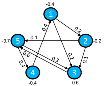
References

  • [1] H. V. Jagadish, J. Gehrke, A. Labrinidis, Y. Papakonstantinou, J. M. Patel, R. Ramakrishnan, and C. Shahabi, “Big data and its technical challenges,” Commun. ACM, vol. 57, no. 7, pp. 86–94, 2014.
  • [2] S. C. Hoi, D. Sahoo, J. Lu, and P. Zhao, “Online learning: A comprehensive survey,” Neurocomput., vol. 459, pp. 249–289, 2021.
  • [3] A. Bifet, R. Gavaldà, G. Holmes, and B. Pfahringer, Machine Learning for Data Streams: with Practical Examples in MOA. Cambridge, MA, USA: MIT Press, 2018.
  • [4] S. Shalev-Shwartz et al., “Online learning and online convex optimization,” Found. Trends Mach. Learn., vol. 4, no. 2, pp. 107–194, 2012.
  • [5] E. Hazan, “Introduction to online convex optimization,” Found. Trends Mach. Learn., vol. 2, no. 3-4, pp. 157–325, 2016.
  • [6] H. Yu, M. Neely, and X. Wei, “Online convex optimization with stochastic constraints,” in Adv. Neural Inf. Process. Syst., vol. 30, pp. 1428–1438, 2017.
  • [7] C. Song, T. Ristenpart, and V. Shmatikov, “Machine learning models that remember too much,” in Proc. 2017 ACM SIGSAC Conf. Comput. Commun. Secur., pp. 587–601, 2017.
  • [8] Y. Gai and B. Krishnamachari, “Distributed stochastic online learning policies for opportunistic spectrum access,” IEEE Trans. Signal Process., vol. 62, no. 23, pp. 6184–6193, 2014.
  • [9] D. Mateos-Núnez and J. Cortés, “Distributed online convex optimization over jointly connected digraphs,” IEEE Trans. Netw. Sci. Eng., vol. 1, no. 1, pp. 23–37, 2014.
  • [10] S. Shahrampour and A. Jadbabaie, “Distributed online optimization in dynamic environments using mirror descent,” IEEE Trans. Autom. Control, vol. 63, no. 3, pp. 714–725, 2017.
  • [11] S. Lee, A. Nedić, and M. Raginsky, “Stochastic dual averaging for decentralized online optimization on time-varying communication graphs,” IEEE Trans. Autom. Control, vol. 62, no. 12, pp. 6407–6414, 2017.
  • [12] J. Lei, P. Yi, Y. Hong, J. Chen, and G. Shi, “Online convex optimization over erdos-rényi random networks,” in Adv. Neural Inf. Process. Syst., vol. 33, pp. 15591–15601, 2020.
  • [13] X. Yi, X. Li, T. Yang, L. Xie, T. Chai, and H. Karl, “Regret and cumulative constraint violation analysis for distributed online constrained convex optimization,” IEEE Trans. Autom. Control, vol. 68, no. 5, pp. 2875–2890, 2022.
  • [14] K. Lu, G. Jing, and L. Wang, “Online distributed optimization with strongly pseudoconvex-sum cost functions,” IEEE Trans. Autom. Control, vol. 65, no. 1, pp. 426–433, 2019.
  • [15] R. Shokri, M. Stronati, C. Song, and V. Shmatikov, “Membership inference attacks against machine learning models,” in Proc. 2017 IEEE Symp. Secur. Privacy, pp. 3–18, 2017.
  • [16] L. Zhu, Z. Liu, and S. Han, “Deep leakage from gradients,” in Adv. Neural Inf. Process. Syst., vol. 32, pp. 17–31, 2019.
  • [17] C. Zhang, M. Ahmad, and Y. Wang, “ADMM based privacy-preserving decentralized optimization,” IEEE Trans. Inf. Forensics Secur., vol. 14, no. 3, pp. 565–580, 2018.
  • [18] Y. Lu and M. Zhu, “Privacy preserving distributed optimization using homomorphic encryption,” Automatica, vol. 96, pp. 314–325, 2018.
  • [19] C. N. Hadjicostis and A. D. Domínguez-García, “Privacy-preserving distributed averaging via homomorphically encrypted ratio consensus,” IEEE Trans. Autom. Control, vol. 65, no. 9, pp. 3887–3894, 2020.
  • [20] Y. Mo and R. M. Murray, “Privacy preserving average consensus,” IEEE Trans. Autom. Control, vol. 62, no. 2, pp. 753–765, 2016.
  • [21] Y. Lou, L. Yu, S. Wang, and P. Yi, “Privacy preservation in distributed subgradient optimization algorithms,” IEEE Trans. Cybern., vol. 48, no. 7, pp. 2154–2165, 2017.
  • [22] S. Gade and N. H. Vaidya, “Private optimization on networks,” in Proc. 2018 Annu. Am. Control Conf., pp. 1402–1409, 2018.
  • [23] Y. Wang, “Privacy-preserving average consensus via state decomposition,” IEEE Trans. Autom. Control, vol. 64, no. 11, pp. 4711–4716, 2019.
  • [24] C. Altafini, “A system-theoretic framework for privacy preservation in continuous-time multiagent dynamics,” Automatica, vol. 122, p. 109253, 2020.
  • [25] P. Jain, P. Kothari, and A. Thakurta, “Differentially private online learning,” in Proc. 25th Annu. Conf. Learn. Theory, pp. 24–1, 2012.
  • [26] S. Han, U. Topcu, and G. J. Pappas, “Differentially private distributed constrained optimization,” IEEE Trans. Autom. Control, vol. 62, no. 1, pp. 50–64, 2016.
  • [27] R. Shokri and V. Shmatikov, “Privacy-preserving deep learning,” in Proc. 22nd ACM SIGSAC Conf. Comput. Commun. Secur., pp. 1310–1321, 2015.
  • [28] M. Abadi, A. Chu, I. Goodfellow, H. B. McMahan, I. Mironov, K. Talwar, and L. Zhang, “Deep learning with differential privacy,” in Proc. 2016 ACM SIGSAC Conf. Comput. Commun. Secur., pp. 308–318, 2016.
  • [29] Z. Huang, S. Mitra, and N. Vaidya, “Differentially private distributed optimization,” in Proc. 16th Int. Conf. Distrib. Comput. Netw., pp. 1–10, 2015.
  • [30] Y. Xiong, J. Xu, K. You, J. Liu, and L. Wu, “Privacy-preserving distributed online optimization over unbalanced digraphs via subgradient rescaling,” IEEE Trans. Control Netw. Syst., vol. 7, no. 3, pp. 1366–1378, 2020.
  • [31] Q. Lü, X. Liao, T. Xiang, H. Li, and T. Huang, “Privacy masking stochastic subgradient-push algorithm for distributed online optimization,” IEEE Trans. Cybern., vol. 51, no. 6, pp. 3224–3237, 2021.
  • [32] T. Ding, S. Zhu, J. He, C. Chen, and X. Guan, “Differentially private distributed optimization via state and direction perturbation in multiagent systems,” IEEE Trans. Autom. Control., vol. 67, no. 2, pp. 722–737, 2022.
  • [33] Y. Wang and T. Başar, “Decentralized nonconvex optimization with guaranteed privacy and accuracy,” Automatica, vol. 150, p. 110858, 2023.
  • [34] Y. Wang and A. Nedić, “Tailoring gradient methods for differentially-private distributed optimization,” IEEE Trans. Autom. Control, 2023.
  • [35] Y. Wang and A. Nedich, “Differentially-private distributed algorithms for aggregative games with guaranteed convergence,” arXiv preprint arXiv:2209.01486, 2022.
  • [36] P. Kairouz, S. Oh, and P. Viswanath, “Extremal mechanisms for local differential privacy,” in Adv. Neural Inf. Process. Syst., vol. 27, pp. 2879–2887, 2014.
  • [37] P. C. M. Arachchige, P. Bertok, I. Khalil, D. Liu, S. Camtepe, and M. Atiquzzaman, “Local differential privacy for deep learning,” IEEE Internet Things J., vol. 7, no. 7, pp. 5827–5842, 2019.
  • [38] E. Garcelon, V. Perchet, C. Pike-Burke, and M. Pirotta, “Local differential privacy for regret minimization in reinforcement learning,” in Adv. Neural Inf. Process. Syst., vol. 34, pp. 10561–10573, 2021.
  • [39] E. Cyffers and A. Bellet, “Privacy amplification by decentralization,” in Proc. 25th Int. Conf. Artif. Intell. Stat., vol. 151, pp. 5334–5353, 2022.
  • [40] J. Zhu, C. Xu, J. Guan, and D. O. Wu, “Differentially private distributed online algorithms over time-varying directed networks,” IEEE Trans. Signal Inf. Process. Netw., vol. 4, no. 1, pp. 4–17, 2018.
  • [41] H. Wang, K. Liu, D. Han, S. Chai, and Y. Xia, “Privacy-preserving distributed online stochastic optimization with time-varying distributions,” IEEE Trans. Control Netw. Syst., vol. 10, no. 2, pp. 1069–1082, 2022.
  • [42] F. Yan, S. Sundaram, S. Vishwanathan, and Y. Qi, “Distributed autonomous online learning: Regrets and intrinsic privacy-preserving properties,” IEEE Trans. Knowl. Data Eng., vol. 25, no. 11, pp. 2483–2493, 2012.
  • [43] C. Li, P. Zhou, L. Xiong, Q. Wang, and T. Wang, “Differentially private distributed online learning,” IEEE Trans. Knowl. Data Eng., vol. 30, no. 8, pp. 1440–1453, 2018.
  • [44] A. I. Maass, C. Manzie, D. Nesic, J. H. Manton, and I. Shames, “Tracking and regret bounds for online zeroth-order euclidean and riemannian optimization,” SIAM J. Optim., vol. 32, no. 2, pp. 445–469, 2022.
  • [45] L. Madden, S. Becker, and E. Dall’Anese, “Bounds for the tracking error of first-order online optimization methods,” J. Optim. Theory Appl., vol. 189, no. 2, pp. 437–457, 2021.
  • [46] A. Simonetto, “Dual prediction–correction methods for linearly constrained time-varying convex programs,” IEEE Trans. Autom. Control., vol. 64, no. 8, pp. 3355–3361, 2019.
  • [47] S. M. Fosson, “Centralized and distributed online learning for sparse time-varying optimization,” IEEE Trans. Autom. Control., vol. 66, no. 6, pp. 2542–2557, 2021.
  • [48] R. H. L. Sim, Y. Zhang, B. K. H. Low, and P. Jaillet, “Collaborative bayesian optimization with fair regret,” in Proc. 38th Int. Conf. Mach. Learn., pp. 9691–9701, 2021.
  • [49] B. Haydon, K. D. Mishra, P. Keyantuo, D. Panagou, F. Chow, S. Moura, and C. Vermillion, “Dynamic coverage meets regret: Unifying two control performance measures for mobile agents in spatiotemporally varying environments,” in Proc. 2021 IEEE Conf. Decis. Control, pp. 521–526, 2021.
  • [50] F. Gao, X. Song, L. Jian, and X. Liang, “Toward budgeted online kernel ridge regression on streaming data,” IEEE Access, vol. 7, pp. 2169–3536, 2019.
  • [51] J. Llavona, Approximation of Continuously Differentiable Functions. North-Holland Mathematics Studies 130, New York: North-Holland, 1986.
  • [52] Z. Pan, Z. Gu, X. Jiang, G. Zhu, and D. Ma, “A modular approximation methodology for efficient fixed-point hardware implementation of the sigmoid function,” IEEE Trans. Ind. Electron., vol. 69, no. 10, pp. 10694–10703, 2022.
  • [53] Z. Leng, M. Tan, C. Liu, E. D. Cubuk, J. Shi, S. Cheng, and D. Anguelov, “Polyloss: A polynomial expansion perspective of classification loss functions,” in Proc. 2022 Int. Conf. Learn. Represent.
  • [54] K. L. Chung, “On a stochastic approximation method,” Ann. Math. Stat., vol. 25, no. 3, pp. 463–483, 1954.
  • [55] “Classification and regression datasets.” https://www.csie.ntu.edu.tw/~cjlin/libsvmtools/datasets/.
  • [56] Y. LeCun, “The MNIST database of handwritten digits,” 1998.
  • [57] A. Krizhevsky, V. Nair, and G. Hinton, “Cifar-10 (canadian institute for advanced research),” 2010.