Leveraging Brain Modularity Prior for Interpretable Representation Learning of fMRI

Abstract

Resting-state functional magnetic resonance imaging (rs-fMRI) can reflect spontaneous neural activities in brain and is widely used for brain disorder analysis. Previous studies propose to extract fMRI representations through diverse machine/deep learning methods for subsequent analysis. But the learned features typically lack biological interpretability, which limits their clinical utility. From the view of graph theory, the brain exhibits a remarkable modular structure in spontaneous brain functional networks, with each module comprised of functionally interconnected brain regions-of-interest (ROIs). However, most existing learning-based methods for fMRI analysis fail to adequately utilize such brain modularity prior. In this paper, we propose a Brain Modularity-constrained dynamic Representation learning (BMR) framework for interpretable fMRI analysis, consisting of three major components: (1) dynamic graph construction, (2) dynamic graph learning via a novel modularity-constrained graph neural network (MGNN), (3) prediction and biomarker detection for interpretable fMRI analysis. Especially, three core neurocognitive modules (i.e., salience network, central executive network, and default mode network) are explicitly incorporated into the MGNN, encouraging the nodes/ROIs within the same module to share similar representations. To further enhance discriminative ability of learned features, we also encourage the MGNN to preserve the network topology of input graphs via a graph topology reconstruction constraint. Experimental results on 534 subjects with rs-fMRI scans from two datasets validate the effectiveness of the proposed method. The identified discriminative brain ROIs and functional connectivities can be regarded as potential fMRI biomarkers to aid in clinical diagnosis.

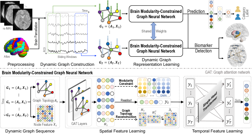
Figure 1: Illustration of the proposed Brain Modularity-constrained dynamic Representation learning (BMR) framework for interpretable functional MRI analysis, including three major components: (1) dynamic graph construction using sliding windows, (2) dynamic graph representation learning via a novel modularity-constrained graph neural network (MGNN), and (3) prediction and biomarker detection for interpretable brain disorder analysis. The BMR is constrained by three fundamental neurocognitive modules, i.e., salience network (SN), central executive network (CEN), and default mode network (DN). To further enhance discriminative ability of learned fMRI representations, we also encourage BMR to reconstruct network topology of input graphs.

1 Introduction

Resting-state functional magnetic resonance imaging (rs-fMRI) provides a noninvasive solution to reveal brain spontaneous neural activities by measuring blood-oxygenation-level-dependent (BOLD) signals [6, 40, 44]. It has been increasingly used to understand underlying neuropathological mechanisms of various brain disorders, such as autism spectrum disorder and cognitive impairment [31, 30, 12]. Many machine/deep learning-based methods have been proposed to map 4D fMRI data into low-dimensional representations and perform downstream brain disease detection [38, 2, 4]. However, due to the complexity of brain organization and the black-box property of many learning-based methods, the generated fMRI representations usually lack biological interpretability, thereby limiting their clinical practicability [16, 7].

From the perspective of graph theory, the human brain exhibits a significant modular structure in spontaneous brain functional networks (BFN), with each module executing specialized cognitive function [18]. A functional module can be defined as a subnetwork of densely interconnected brain regions-of-interest (ROIs) that are sparsely connected to ROIs in other modules [45, 35]. In particular, salience network (SN), central executive network (CEN), and default mode network (DMN) are three fundamental neurocognitive modules/subnetworks in human brains, supporting effective cognitive activities [17]. Unfortunately, existing fMRI-based studies usually fail to adequately utilize such brain modularity prior during fMRI representation learning. On the other hand, the brain can be modeled as a spatiotemporally dynamic BFN (i.e., dynamic graph) based on BOLD signals, aiming to help simultaneously capture spatial and temporal information of brain neural activities [27, 13]. Intuitively, it is meaningful to incorporate brain modularity prior into a dynamic graph representation framework for interpretable fMRI analysis.

To this end, we propose a Brain Modularity-constrained dynamic Representation learning (BMR) framework for interpretable fMRI analysis. As shown in the top panel of Fig. 1, the proposed BMR consists of three major components: (1) dynamic graph construction using sliding windows, (2) dynamic graph representation learning via a novel brain modularity-constrained graph neural network (MGNN), and (3) prediction and biomarker detection for interpretable fMRI analysis. In particular, three core neurocognitive modules (i.e., SN, CEN, and DMN) are explicitly incorporated into the BMR through our proposed modularity constraint, encouraging learned features of ROIs within the same module to be similar. To enhance discriminative ability of learned features, we design a graph topology reconstruction constraint to encourage our BMR to preserve the network topology of input graphs during fMRI feature learning. Experimental results on 534 subjects with rs-fMRI from the public Autism Brain Imaging Data Exchange (ABIDE) dataset [10] and a private HIV-associated neurocognitive disorder (HAND) dataset demonstrate the superiority of the proposed BMR over several state-of-the-art methods for brain disorder detection.

The contributions of this work are summarized as follows.

• A novel brain modularity-constrained dynamic representation learning framework is designed for interpretable fMRI analysis, where brain ROIs within the same functional module are encouraged to share similar representations. To the best of our knowledge, this is among the first attempts to incorporate brain modularity prior into graph neural networks for fMRI analysis.

• A graph reconstruction constraint is introduced during dynamic graph learning to preserve original topology information of brain functional networks, thus enhancing discriminative ability of learned fMRI features.

• Our BMR is a general framework that can be applied to fMRI-based analysis of different brain disorders, such as autism spectrum disorder and HIV-associated neurocognitive disorder, as evidenced by its superior performance on ABIDE [10] and a private HAND dataset.

2 Related Work

2.1 Functional MRI Representation Learning

Various machine learning methods have been used to learn latent representations of resting-state fMRI for brain disorder analysis [22]. For example, Wee et al.  [48] proposed a constrained sparse linear regression model to estimate brain functional network (BFN) for mild cognitive impairment classification with resting-state fMRI. Rosa et al.  [41] designed a sparse network-based predictive model that first constructed sparse inverse covariance matrices and then used a sparse support vector machine (SVM) for major depressive disorder detection. Gan et al.  [15] proposed a multi-graph fusion method that first integrated fully-connected BFNs and one nearest neighbor BFNs and then employed the L1SVM for brain disorder classification.However, these existing studies generally treat fMRI feature learning and downstream model training as two standalone steps, possibly leading to suboptimal performance due to heterogeneity between these steps.

Deep learning methods have been widely used for computer-aided brain disorder diagnosis with fMRI [50], by jointly conducting fMRI representation learning and downstream model training in an end-to-end manner. In particular, due to the graph structure nature of BFN, graph neural networks (GNNs) have shown significant superiority in fMRI representation learning. For example, Ktena et al.  [29] proposed a siamese graph convolutional network (GCN) to estimate BFN for automated autism analysis. Jiang et al.  [21] designed a hierarchical GCN framework for BFN embedding learning by efficiently integrating correlations among subjects in a population. Hu et al.  [20] designed a complementary graph representation learning method to capture local and global patterns for fMRI-based brain disease analysis. Although these GNN-based methods can model spatial interactions among brain ROIs, they often neglect dynamic variations over time of fMRI data. Considering that temporal dynamics conveyed in fMRI can provide discriminative information for brain disease diagnosis, some GNN-based studies have paid more attention to spatiotemporally dynamic brain network analysis with fMRI data. For instance, Gadgil et al.  [13] introduced a novel spatiotemporal GCN, which captured temporal dynamics within fMRI series via 1D convolutional kernels, to learn dynamic grap representation for age and gender prediction. Even achieving promising results in fMRI representation learning, most of existing GNN models cannot explicitly preserve network topology of BFNs during dynamic graph learning.

2.2 Brain Functional Modularity Analysis

From a graph-theoretic perspective, the BFN during the resting state exhibits a significant modular structure to facilitate efficient information communication and cognitive function [35, 45]. To better understand brain connectivity patterns, researchers have devoted considerable attention to analyzing brain modularity. For example, Meunier et al.  [34] explored age-related changes in brain modular organization and demonstrated significantly non-random modularity in young and older brain networks. Arnemann et al.  [1] tested the value of modularity metric to predict response to cognitive training after brain injury. Gallen et al.  [14] demonstrated that brain modularity could be regarded as a unifying biomarker of intervention-related plasticity by multiple independent studies.

Notably, previous neuroscience studies have demonstrated that there are three fundamental cognitive modules, i.e., salience network (SN), central executive network (CEN), and default mode network (DMN) in human brains. Specifically, SN mainly detects external stimuli and coordinates brain neural resources, CEN performs high-level cognitive tasks (e.g., decision-making and rule-based problem-solving), while DMN is responsible for self-related cognitive functions (e.g., mind-wandering and introspection) [17, 33]. These three modules have been consistently observed across different individuals and experimental paradigms [33, 28]. For example, Menon et al.  [33] proposed a unifying triple network model comprised of CEN, DMN, and SN, providing a common framework for understanding behavioral and cognitive dysfunction across multiple brain disorders. Krishnadas et al.  [28] investigated disrupted resting-state functional connectivities within the triple network in patients with paranoid schizophrenia. Intuitively, such brain modularity structures can be employed as important prior knowledge to promote informative fMRI feature learning. However, existing studies typically fail to incorporate such important modularity prior into deep graph learning models for fMRI-based brain disorder analysis.

3 Materials

3.1 Data Acquisition

A total of 534 subjects with rs-fMRI scans from the public Autism Brain Imaging Data Exchange (ABIDE) dataset [10] and a private HIV-associated neurocognitive disorder (HAND) dataset are used in this work. On ABIDE, we identify patients with autism spectrum disorder (ASD) from healthy control (HC) subjects on the two largest sites (i.e., NYU and UM). Specifically, the NYU site includes $79$ ASDs and $105$ HCs, and the UM site includes $68$ ASDs and $77$ HCs. On HAND, we perform two kinds of classification tasks, including (1) asymptomatic neurocognitive impairment with HIV (ANI) vs. HC classification, and (2) intact cognition with HIV (ICH) vs. HC classification. Here, rs-fMRI data in the HAND are collected from a local hospital, including $67$ ANIs, $68$ ICHs and $70$ HCs. The demographic information of the studied subjects from two datasets is reported in Table 1.

Table 1: Demographic information of subjects from two largest sites (i.e., NYU and UM) of ABIDE dataset and a private HAND dataset. ASD: autism spectrum disorder; HC: healthy control; ANI: asymptomatic neurocognitive impairment with HIV; ICH: intact cognition with HIV; M: Male; F: Female; Std: Standard deviation.

Dataset	Site	Category	Subject #	Gender (M/F)	Age (Mean$\pm$Std)
ABIDE	NYU	ASD	$79$	$68$/$11$	$14.52\pm 6.97$
		HC	$105$	$79$/$26$	$15.81\pm 6.25$
	UM	ASD	$68$	$58$/$10$	$13.13\pm 2.41$
		HC	$77$	$59$/$18$	$14.79\pm 3.57$
HAND	–	ANI	$67$	$67$/$0$	$33.07\pm 6.18$
		ICH	$68$	$68$/$0$	$33.40\pm 5.58$
		HC	$70$	$70$/$0$	$33.33\pm 5.37$

3.2 Data Preprocessing

All rs-fMRI data from two datasets were preprocessed using the Data Processing Assistant for Resting-State fMRI (DPARSF) pipeline [49]. Specifically, for each fMRI, we first discarded the first 10 time points for magnetization equilibrium. Then, we performed slice timing correction, head motion correction, and regression of nuisance covariates (e.g., white matter signals, ventricle, and head motion parameters). Afterward, the fMRI data were normalized into montreal neurological institute (MNI) space, followed by spatial smoothing with a $4\,mm$ full width half maximum Gaussian kernel and band-pass filtering ($0.01-0.1\,Hz$). Finally, we extracted the mean rs-fMRI time series of $116$ ROIs defined by the automated anatomical labeling (AAL) atlas for each subject.

4 Proposed Methodology

As illustrated in Fig. 1, the proposed BMR is comprised of three major components: (1) dynamic graph construction using sliding windows, (2) dynamic graph learning via a novel brain modularity-constrained graph neural network (MGNN), and (3) prediction and biomarker detection for interpretable brain disorder analysis, with details presented below.

4.1 Dynamic Graph Construction

Brain functional network (BFN) derived from fMRI data can capture abnormal connectivity patterns caused by brain disorders by modeling complex dependencies among brain ROIs. Given the fact that brain functional connectivity exhibits dynamic variability over a short period of time [13], we construct a dynamic BFN using sliding windows for each subject [32]. Denote BOLD signals obtained from rs-fMRI as $S\in\mathbb{R}^{N\times M}$, where $N$ is the number of ROIs and $M$ is the number of time points. We first partition the fMRI time series into $T$ segments along the temporal dimension via overlapped sliding windows, with the window size of $\Gamma$ and the step size of $\tau$. With each ROI treated as a specific node, we construct a fully-connected BFN by calculating Pearson correlation coefficients [42] between segmented fMRI time series of pairwise brain ROIs for each of $T$ segments, obtaining a set of symmetric matrices $\{X_{t}\}_{t=1}^{T}\in\mathbb{R}^{N\times N}$. Here, the original node feature for the $j$-th node is represented by the $j$-th row in $X_{t}$ for segment $t$ ($X_{t}$ is also called node feature matrix). Considering that a fully-connected BFN may contain some noisy or redundant information, following [24], we empirically retain the top $30\%$ (i.e., sparsity ratio) strongest edges in each FC network to generate an adjacent matrix $A_{t}=(a_{ij})\in\{0,1\}^{N\times N}$ for the segment $t$, where $a_{ij}=1$ means there exists an edge between two nodes/ROIs and otherwise $a_{ij}=0$. Finally, the obtained dynamic graph sequence of each subject can be described as $G_{t}=\{A_{t},X_{t}\}~{}(t=1,\cdots,T)$.

4.2 Dynamic Graph Representation Learning via MGNN

As illustrated in the bottom of Fig. 1, with the constructed dynamic graph sequence $\{G_{t}\}_{t=1}^{T}$ as input, we design a brain modularity-constrained graph neural network (MGNN) for dynamic fMRI representation learning, including (1) spatial feature learning and (2) temporal feature learning, which can simultaneously model spatial dependencies among brain ROIs and temporal dynamics over time. Notably, a novel brain modularity constraint and a graph topology reconstruction constraint are incorporated into MGNN to learn more interpretable and discriminative graph representations.

4.2.1 Spatial Feature Learning

Considering the graph-structured property of BFNs, we employ a graph attention network (GAT) as the spatial feature encoder to model spatial dynamic representation of BFNs in this work. Taking the segment $t$ as an example, the spatial encoder takes the node feature matrix $X_{t}=[X_{1}^{t},X_{2}^{t},\cdots,X_{N}^{t}]^{\top}$ ($X_{i}^{t}\in\mathbb{R}^{1\times N}$) and the graph adjacent/topology matrix $A_{t}$ as input. Denote $\mathcal{N}_{i}^{t}$ as the neighboring node set of the $i$-th node and $\oplus$ as the concatenation operation. The to-be-learned connection weight (also called spatial attention coefficient) between the $i$-th ROI and its neighborhood ROI $j$ can be formulated as:

$$\alpha^{t}_{ij}=\frac{{exp}\left(\psi([X_{i}^{t}W^{t}\oplus X_{j}^{t}W^{t}]\eta^{t})\right)}{\sum\nolimits_{v\in\mathcal{N}_{i}^{t}}{exp}\left(\psi([X_{i}^{t}W^{t}\oplus X_{v}^{t}W^{t}]\eta^{t})\right)},$$ (1)

where $\psi$ is a nonlinear activation function (i.e., LeakyRelu), $W^{t}\in\mathbb{R}^{N\times N^{\prime}}$ is a shared transformation matrix that maps the original $N$-dimensional node feature vector to an $N^{\prime}$-dimensional vector, and ${{\eta^{t}}\in\mathbb{R}^{2N^{\prime}}}$ is a to-be-learned weight vector. Then, the updated node representation is expressed as:

$$F_{i}^{t}=\sum\nolimits_{j\in\mathcal{N}_{i}^{t}}\alpha^{t}_{ij}X_{j}^{t}W^{t},$$ (2)

where $F_{i}^{t}\in\mathbb{R}^{1\times N^{\prime}}$ is the new embedding of the node $i$ after aggregating neighboring node representations. To model different types of spatial dependencies/relationships among ROIs/nodes, we employ a multi-head attention mechanism, which first calculates node representation using multiple attention heads in parallel and then averages them. Mathematically, the output feature $H_{i}^{t}\in\mathbb{R}^{1\times N^{\prime}}$ of the node $i$ generated by the multi-head attention mechanism can be written as follows:

$$H_{i}^{t}=\sigma(\frac{1}{K}\sum\nolimits_{k=1}^{K}{F_{i}^{t,k}}),$$ (3)

where $\sigma$ is a nonlinear function and $K$ is the number of attention heads. Given $N$ nodes, the new node-level embedding of BFN can be expressed as $H^{t}=[H_{1}^{t},\cdots,H_{N}^{t}]^{\top}$ at segment $t$.

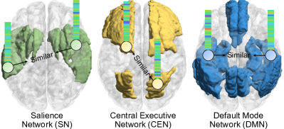
Figure 2: Illustration of the proposed modularity constraint with three fundamental cognitive modules, i.e., salience network (SN), central executive network (CEN), and default mode network (DMN), where nodes within the same module are encouraged to share similar representation.

(1) Brain Modularity Constraint. As an important property of BFN [14], modularity provides valuable insights into the organization and integration of brain networks. In general, each module is comprised of densely interconnected brain ROIs that are sparsely connected to ROIs in other modules [45]. Due to the high clustering of connections between ROIs within the module, the brain can locally process specialized cognitive function (i.e., episodic memory processing) with low wiring cost [35]. Previous studies have demonstrated that SN, CEN, and DMN are three fundamental neurocognitive modules in human brains. Based on such prior knowledge, we reasonably assume that representations of nodes within the same neurocognitive module tend to be similar to each other.

Accordingly, we design a unique brain modularity constraint during spatial fMRI feature learning in BMR. As illustrated in Fig. 2, the modularity constraint explicitly encourages the nodes belonging to the same module to share similar features. Based on Cosine distance metric, this constraint can be mathematically formulated as follows:

$$\small L_{M}=-\sum\nolimits_{t=1}^{T}\sum\nolimits_{c=1}^{C}\sum\nolimits_{i,j=1}^{N_{c}}\frac{H_{i}^{t,c}\cdot H_{j}^{t,c}}{\|H_{i}^{t,c}\|\cdot\|H_{j}^{t,c}\|},$$ (4)

where $H_{i}^{t,c}$ and $H_{j}^{t,c}$ are representations of node $i$ and node $j$ within the $c$-th module (with $N_{c}$ ROIs) at segment $t$, and $C$ is the number of modules ($C=3$ in this work). With Eq. (4), we encourage the BMR to focus on brain intrinsic modular organization during fMRI representation learning, thus enhancing discriminative power of learned fMRI features.

(2) Graph Topology Reconstruction Constraint. To further improve discriminative ability of learned representations, we propose to preserve original topology information of input BFNs by reconstructing the adjacent matrix $A_{t}$ at segment $t$ ($t=1,\cdots,T$). Motivated by variational graph autoencoder [26], we design a graph decoder in BMR to first predict the presence of edges between pairwise nodes based on the inner-product of two latent node representations, yielding a reconstructed adjacent matrix $\hat{A}_{t}=\sigma(H_{t}\cdot H_{t}^{\top})$ for segment $t$, where $\sigma$ is a nonlinear mapping function. We then propose a graph topology reconstruction constraint to preserve network topology of input BFNs, formulated as:

$$\small L_{R}=\sum\nolimits_{t=1}^{T}\xi({A}_{t},\hat{A}_{t}),$$ (5)

where $\xi$ is a cross-entropy loss function. With Eq. 5, the reconstructed graph is encouraged to closely resemble the original graph as far as possible, so that the learned node embeddings can effectively capture underlying FCN structure and relationships among ROIs.

To generate graph-level representations, we further apply a squeeze-excitation readout operation [19] based on learned node-level representations. For segment $t$, the graph-level spatial representation is calculated as:

$$y_{t}=H_{t}\Phi\left(P^{2}\sigma(P^{1}H_{t}\phi_{mean})\right),$$ (6)

where $\Phi$ is a sigmoid function, $P^{1}$ and $P^{2}$ are learnable weight matrices, and $\phi_{mean}$ denotes the average operation.

4.2.2 Temporal Feature Learning

As shown in the bottom right of Fig. 1, to further capture temporal dynamics within fMRI series, a single-head transformer encoder is employed to effectively model long-range dependencies across different segments. Here, temporal attention can be measured by a self-attention mechanism in the transformer. Especially, with spatial graph representations $Y=[y_{1},\cdots,y_{T}]$ as input, temporal attention weights can be described as:

$$Z=Softmax(\frac{QK^{\top}}{\sqrt{d}}),\small$$ (7)

where $Q=\phi_{1}(Y)$, $K=\phi_{2}(Y)$, $\phi_{1}$ and $\phi_{2}$ are two linear transformations, $d$ is a scaling factor to stabilize attention mechanism. Thus, the graph representation with spatiotemporal attention can be expressed as $Y^{\prime}=\Psi[Z\phi_{3}(Y)]$, where $Y^{\prime}=[y_{1}^{\prime},\cdots,y_{T}^{\prime}]$, $\phi_{3}$ is a linear transformation, and $\Psi$ represents the feed-forward network for further feature abstraction. After that, we sum the updated graph representation sequence $\{{y}_{i}^{\prime}\}_{i=1}^{T}$ to obtain the final whole-graph embedding for subsequent brain disorder analysis.

Table 2: Classification results of competing methods and the proposed BMR on the two largest sites of ABIDE. Results are shown in the form of “mean(standard deviation)” and the best results are shown in bold. The term ‘*’ represents the proposed BMR is statistically significantly different from a competing method.

Method	ASD vs. HC classification on NYU							ASD vs. HC classification on UM
	AUC (%)	ACC (%)	F1 (%)	SEN (%)	SPE (%)	BAC (%)		AUC (%)	ACC (%)	F1 (%)	SEN (%)	SPE (%)	BAC (%)
SVM	56.64(2.89)∗	54.83(3.11)	48.64(3.38)	51.48(4.56)	57.88(4.66)	54.69(3.09)		53.61(4.25)∗	53.32(3.63)	49.32(4.20)	50.29(4.53)	56.60(4.66)	53.45(3.76)
XGBoost	61.95(0.56)∗	63.00(1.63)	51.49(1.84)	47.99(2.68)	75.91(3.72)	61.95(0.56)		58.81(0.83)∗	58.62(1.89)	50.19(1.95)	47.61(3.64)	70.01(3.94)	58.81(0.84)
Random Forest	61.21(3.09)∗	61.10(4.48)	49.31(4.62)	46.04(4.12)	74.06(5.23)	60.05(4.67)		57.25(2.77)∗	56.13(3.66)	49.25(4.87)	47.73(5.83)	65.68(4.11)	56.70(4.04)
MLP	58.64(2.51)∗	58.28(1.60)	46.66(4.39)	45.22(7.22)	68.24(5.48)	56.73(1.64)		58.17(2.89)∗	54.48(3.00)	48.06(1.81)	47.67(2.47)	62.70(5.99)	55.19(2.78)
GCN	67.53(3.34)	63.59(3.05)	53.63(3.75)	50.99(5.09)	73.54(4.69)	62.26(2.82)		66.74(2.58)∗	60.00(2.96)	55.30(3.07)	54.61(4.42)	66.50(5.22)	60.56(2.57)
GIN	61.43(3.45)∗	57.04(2.48)	48.24(2.13)	49.35(5.39)	64.94(5.70)	57.14(1.16)		58.94(3.19)∗	56.89(2.73)	50.47(2.73)	49.62(3.23)	64.92(3.41)	57.27(2.40)
GAT	64.87(2.64)∗	60.12(2.64)	52.14(3.83)	52.96(4.92)	66.12(3.15)	59.54(2.79)		67.34(3.26)∗	60.90(3.58)	55.54(4.59)	54.98(5.39)	68.21(5.15)	61.60(2.95)
BrainGNN	66.89(2.90)∗	63.21(3.15)	56.31(4.17)	57.12(4.81)	68.51(3.03)	62.82(3.24)		65.91(2.47)	62.69(2.55)	57.18(1.21)	55.47(3.25)	68.09(5.67)	61.78(2.06)
STGCN	66.69(0.87)∗	61.54(1.65)	45.55(2.23)	53.64(2.34)	68.42(1.75)	61.03(1.53)		64.01(0.14)∗	63.90(0.10)	44.19(3.91)	55.95(1.18)	72.16(0.56)	64.07(0.14)
BMR (Ours)	73.24(4.48)	67.10(4.29)	62.16(4.53)	64.74(5.08)	69.39(6.22)	67.06(4.38)		70.55(5.22)	65.28(2.37)	62.25(2.14)	63.21(2.71)	67.42(4.79)	65.31(3.08)

Table 3: Classification results of competing methods and the proposed BMR on HAND. Results are shown in the form of “mean(standard deviation)” and the best results are shown in bold. The term ‘*’ represents the proposed BMR is statistically significantly different from a competing method.

Method	ANI vs. HC classification on HAND							ICH vs. HC classification on HAND
	AUC (%)	ACC (%)	F1 (%)	SEN (%)	SPE (%)	BAC (%)		AUC (%)	ACC (%)	F1 (%)	SEN (%)	SPE (%)	BAC (%)
SVM	61.73(3.21)∗	57.28(2.68)	56.25(2.98)	58.25(4.27)	57.22(2.87)	57.73(2.72)		53.91(3.54)∗	52.52(4.75)	51.86(5.61)	53.95(6.29)	51.50(7.25)	52.73(5.14)
XGBoost	56.72(3.59)∗	53.34(2.83)	51.11(2.82)	51.70(3.61)	56.70(6.59)	54.21(2.76)		55.05(3.66)∗	53.04(2.19)	51.29(2.27)	52.34(3.46)	55.55(3.51)	53.95(1.92)
Random Forest	64.64(1.46)	58.61(1.54)	57.88(3.03)	60.49(5.13)	59.51(5.45)	60.00(1.52)		57.11(4.23)∗	53.10(4.79)	51.70(3.95)	53.31(4.81)	55.89(8.04)	54.60(4.70)
MLP	64.68(3.82)∗	58.97(2.69)	57.37(2.49)	59.05(2.82)	59.55(3.85)	59.30(2.28)		56.44(4.02)	55.25(3.40)	55.81(2.55)	59.30(2.09)	52.24(6.86)	55.77(3.40)
GCN	64.23(2.13)∗	59.60(2.32)	57.78(3.29)	58.65(5.06)	61.65(4.89)	60.15(2.39)		55.42(6.44)∗	54.65(1.49)	53.08(5.09)	55.60(9.52)	53.63(10.20)	54.62(1.60)
GIN	65.93(3.61)∗	60.34(2.25)	58.40(3.06)	59.00(4.57)	62.36(3.49)	60.68(2.72)		57.78(3.60)∗	54.80(3.69)	53.78(4.11)	55.90(4.58)	56.39(4.04)	56.14(3.21)
GAT	65.72(3.86)∗	61.11(2.99)	59.24(0.78)	62.53(5.83)	59.47(6.00)	61.00(0.09)		54.42(3.01)∗	53.67(4.03)	54.41(4.00)	60.06(8.78)	50.12(7.77)	55.09(4.57)
BrainGNN	63.04(3.23)∗	60.26(2.60)	56.87(3.78)	56.32(5.95)	63.70(5.59)	60.01(1.78)		58.14(4.75)	56.74(2.23)	57.38(2.84)	61.48(3.80)	51.20(3.45)	56.34(2.36)
STGCN	53.81(2.94)∗	51.20(4.00)	52.45(3.78)	57.40(5.45)	47.40(5.64)	52.40(4.02)		55.22(8.36)∗	51.11(7.62)	50.88(10.36)	55.34(22.93)	49.48(8.16)	52.41(8.40)
BMR (Ours)	67.91(3.49)	64.03(4.97)	61.78(6.89)	62.39(8.68)	66.25(3.81)	64.32(5.16)		60.26(4.98)	57.49(4.15)	55.15(5.58)	54.82(7.26)	61.12(6.94)	57.97(4.34)

4.3 Prediction and Interpretable Biomarker Detection

The whole-graph embedding is then fed into two fully connected layer and a Softmax layer for brain disease prediction. The objective function of our BMR can be formulated as:

$$\small L=L_{C}+\lambda_{1}L_{R}+\lambda_{2}L_{M},$$ (8)

where $L_{C}$ is a cross-entropy loss for prediction, $L_{R}$ and $L_{M}$ denote the proposed graph topology reconstruction constraint and brain modularity constraint, respectively, while $\lambda_{1}$ and $\lambda_{2}$ are two hyperparameters.

To facilitate interpretation of our learned graph representations, we further analyze spatial attention among brain ROIs, which can provide potential biomarkers for brain disorder diagnosis. Specifically, based on spatial attention coefficients described in Eq. 1, we first obtain spatial attention matrices of $T$ segments and average them to generate a spatial attention matrix for each subject. Then, we take the upper triangle elements of each attention matrix, resulting in a $6,670$-dimensional vector. Finally, we employ $t$-test to select discriminative features by calculating group differences between patients and healthy controls, and also map these features to their original brain space to detect the most discriminative functional connectivities in brain disease detection. The specific biomarker analysis will be introduced in Section 6.1

4.4 Implementation Details

The proposed BMR is implemented in PyTorch using a single GPU (NVIDIA TITAN Xp with 12GB memory). The Adam optimizer is used for optimization, with the learning rate of $0.0001$, training epochs of $40$, batch size of $8$, window size of $\Gamma=40$ and step size of $\tau=20$. Within the $c$-th module (with $N_{c}$ ROIs), we randomly select $m=50\%$ of all $\frac{N_{c}(N_{c}-1)}{2}$ paired ROIs to constrain the BMR. The hyperparameters (i.e., $\lambda_{1}$ and $\lambda_{2}$) in Eq. (8) are determined via a cross-validation strategy (see Section 5.1 and Section 6.2).

5 Experiments

5.1 Experimental Settings

A 5-fold cross-validation (CV) strategy is employed in the experiments. Besides, within each fold, we randomly select 20% of training samples as the validation set to determine the optimal parameters. We repeat above 5-fold CV process five times to avoid bias caused by data partition and record the mean and standard deviation results. Six metrics are used to evaluate classification performance, including the area under the receiver operating characteristic curve (AUC), classification accuracy (ACC), F1 score (F1), sensitivity (SEN), specificity (SPE), and balanced accuracy (BAC). Paired sample $t$-test is used to perform statistical significance analysis between the BMR and each of competing methods.

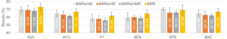
Figure 3: Performance of the BMR and its three variants in ASD vs. HC classification on NYU site of ABIDE dataset.

5.2 Competing Methods

We compare the proposed BMR with three conventional machine learning methods: SVM [39], XGBoost [8], and Random Forest [5], as well as six deep learning methods: multilayer perceptron (MLP) [37], GCN [25], graph isomorphism network (GIN) [23], graph attention network (GAT) [46], BrainGNN [31], and spatio-temporal graph convolutional network (STGCN) [13], with details introduced below.

(1) SVM: In this method, we first construct a BFN based on rs-fMRI for each subject by measuring Pearson correlation (PC) coefficients between pairwise brain ROIs. Then, we extract multiple node statistics (i.e., degree centrality, clustering coefficient, betweenness centrality, and eigenvector centrality) of each BFN and concatenate them into a $464$-dimensional vector. Finally, the vectorized fMRI representation is fed into a linear SVM (with default parameter $C=1$) for classification.

(2) XGBoost: Similar to SVM, we first construct a BFN based on PC for each subject and then concatenate the same node statistics into a vectorized representation, followed by XGBoost (with default parameters) for classification.

(3) Random Forest: This method uses the same fMRI features as SVM and XGBoost, followed by a random forest classifier (with default parameters).

(4) MLP: Similar to above three methods, we first extract node features to represent each subject, and then use two fully connected layers for feature abstraction and a Softmax layer for brain disorder prediction.

(5) GCN: In this method, we first construct a BFN using PC for each subject. Then, two graph convolutional layers are used to update and aggregate node-level representations. Finally, graph-level representations are generated via readout operation based on node representations, followed by two fully connected layers for classification.

(6) GIN: Similar to GCN, this method first constructs a BFN for each subject and then uses two GIN layers that implement Weisfeiler-Lehman graph isomorphism test in a neural network for feature learning. Finally, we obtain graph representations via a readout operation, followed by two fully connected layers and a Softmax layer for classification.

(7) GAT: Different from GCN and GIN, the GAT uses a graph attention mechanism to learn adaptive edge weights between brain ROIs. In this method, we use two graph attention layers to learn spatial features, a readout operation to generate graph-level vectors, two fully connected layers, and a Softmax layer for classification. Similar to our BMR, the number of attention heads is $4$ for each graph attention layer.

(8) BrainGNN: BrainGNN is a popular GNN model specially designed for fMRI analysis, containing an ROI-selection layer for highlighting salient brain ROIs. With constructed BFNs as input, BrainGNN uses two ROI-aware graph convolutional layers to learn node embeddings, followed by ROI pooling layers to reduce the size of graph. Then, a readout operation is used to convert node-level features into graph-level representations, followed by two fully connected layers and a Softmax layer for classification.

(9) STGCN: The STGCN can jointly capture spatial and temporal information of FCNs via spatiotemporal graph convolution (ST-GC) units. In this method, we first employ two ST-GC units for learning spatiotemporal features with BOLD signals of ROIs as input. Then, dynamic graph representations are generated via readout operation, followed by two fully connected layers for disease prediction.

For a fair comparison, we use the same number of hidden layers (i.e., 2) and the same number of neurons in each hidden layer (i.e., 64) for five GNN-based methods (i.e., GCN, GIN, GAT, BrainGNN, and STGCN). Additionally, we use the same input BFN data for four GNN-based methods (i.e., GCN, GIN, GAT, and Brain GNN), while the STGCN employs the processed fMRI time series as input.

5.3 Classification Results

The quantitative results of the proposed BMR and nine competing methods on ABIDE and HAND are reported in Table 2 and Table 3, respectively, where ‘*’ represents the proposed BMR is statistically significantly different from a specific competing method via paired sample $t$-test. From Tables 2-3, we have the following interesting observations.

First, our BMR is superior to traditional machine learning methods (i.e., SVM, XGBoost, and Random Forest) by a significant margin on two datasets (i.e., ABIDE and HAND). For example, in terms of AUC values, the BMR yields the improvement of $16.6\%$, $11.29\%$, $12.03\%$ compared with SVM, XGBoost, Random Forest on the NYU site of ABIDE, respectively. The possible reason is that our BMR can learn informative fMRI representation in an end-to-end manner as needed for downstream tasks compared with these traditional methods that rely on handcrafted node features. Second, compared with six deep models (i.e., MLP, GCN, GIN, GAT, BrainGNN, and STGCN), our BMR achieves better performance in terms of most metrics on two datasets. For instance, in the task of ANI vs. HC classification on HAND, the BMR improves the AUC value by $4.87\%$, compared with BrainGNN (a GNN-based model specially designed for brain network analysis). This is probably because our BMR not only focuses more on three inherent functional modules in the brain but also preserves the original topology structure during graph learning, resulting in more discriminative fMRI representation for classification. Furthermore, it can be seen the BMR consistently outperforms STGCN that models short-range temporal dynamics within fMRI via a convolution operation. The possible reason is that our BMR can not only capture long-range temporal dependencies within fMRI series via a transformer encoder, but also incorporate crucial modularity prior into the process of dynamic graph representation learning, thereby achieving better classification performance.

5.4 Ablation Study

To investigate the effectiveness of key components in the proposed method, we compare the BMR with its three variants: (1) BMRw/oM without the modularity constraint, (2) BMRw/oR without the graph topology reconstruction constraint, and (3) BMRw/oMR that only uses GAT and Transformer layers for spatiotemporal representation learning, without the two constraints. The experimental results yielded by these four methods in ASD vs. HC classification on NYU from ABIDE are reported in Fig. 3.

From Fig. 3, we can see that BMR outperforms BMRw/oM without considering the inherent modular structure in the brain. This implies that incorporating brain modularity prior to fMRI representation can help promote classification performance by learning more discriminative features. Besides, the BMR is superior to BMRw/oR without performing graph topology reconstruction during fMRI representation learning. The underlying reason is the proposed graph topology reconstruction constraint helps capture intrinsic spatial information among brain ROIs. In addition, the BMRw/oMR without the proposed two constraints achieves the worst performance in most cases compared with its three counterparts (i.e., BMRw/oM, BMRw/oR, and BMR), which further validates the necessity of including modularity constraint and graph topology constraint.

6 Discussion

6.1 Discriminative Brain ROI and Functional Connectivity

We also visualize the top 10 discriminative functional connectivities (FCs) identified by the proposed BMR on different datasets (i.e., ABIDE and HAND) in Fig. 4. Note that the thickness of each line represents discriminative ability of the corresponding FC (inversely proportional to the $p$-value obtained by $t$-test). For ASD identification (see Fig. 4 (a)), the most discriminative FCs involve anterior cingulate and paracingulate gyri, parahippocampal gyrus, and hippocampus, which complies with previous ASD-related findings [11, 36, 3]. As shown in Fig. 4 (b), the identified discriminative brain ROIs in ANI identification include insula, right temporal pole: superior temporal gyrus, supplementary motor area, and caudate nucleus. These regions have also been reported in previous studies on HIV-related cognitive impairment [52, 51, 43, 9]. These results further demonstrate the effectiveness of the BMR in detecting interpretable disease-associated biomarkers. The identified discriminative brain ROIs and FCs can be regarded as potential biomarkers to aid in clinical diagnosis.

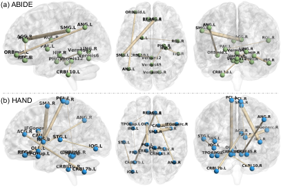
Figure 4: Top ten discriminative functional connectivities identified by our BMR in (a) ASD vs. HC classification on NYU from ABIDE and (b) ANI vs. HC classification on HAND.

6.2 Influence of Hyperparameters

We have two hyperparameters (i.e., $\lambda_{1}$ and $\lambda_{2}$) in the proposed BMR (see Eq. (8)) to control contributions of brain modularity constraint and graph topology reconstruction constraint, respectively. To study their influences on the performance of BMR, we tune $\lambda_{1}$ and $\lambda_{2}$ within the range of $\{10^{-4},10^{-3},\cdots,10^{1}\}$ based on training and validation sets for ASD vs. HC classification on NYU from ABIDE, and report the results of BMR in Fig. 5. It can be observed from Fig. 5 that the BMR with a large $\lambda_{1}$ (e.g., $\lambda_{1}=10$) achieves worse performance. The underlying reason may be that using a strong graph reconstruct constraint will make the model difficult to converge, thus degrading its learning performance. On the other hand, the BMR with a very weak modularity constraint (e.g., $\lambda_{2}=10^{-4}$) is generally inferior to that with relatively stronger modularity constraint (e.g., $\lambda_{2}=10^{-2}$). These results mean that the BMR can not achieve satisfactory performance when the BMR pays less attention to brain inherent modular structure, which further validates the effectiveness of the designed brain modularity constraint. In particular, the BMR achieves the best AUC values with $\lambda_{1}=10^{-2}$ and $\lambda_{2}=10^{-2}$ in this task.

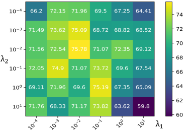
Figure 5: AUC values (%) of the proposed BMR under different hyperparameters (i.e., $\lambda_{1}$ and $\lambda_{2}$) in the task of ASD vs. HC classification on NYU site of ABIDE dataset.

6.3 Influence of Spatial Feature Encoder

In the main experiments, our BMR uses GAT as spatial feature encoder to capture dependencies among brain ROIs. To investigate the influence of the spatial feature encoder, we replace GAT with the graph isomorphism network (GIN) to extract spatial fMI features in BMR, and call this variant as BMR-GIN. The results of BMR and BMR-GIN for ASD vs. HC classification on NYU are reported in Fig. 6. It can be found from Fig. 6 that BMR achieves better performance than BMR-GIN in most cases. The main reason could be that, compared with BMR-GIN that treats neighboring nodes equally during the process of aggregating node features, the BMR can adaptively assign different attention weights to different neighboring nodes so that the model can focus on important nodes, thus improving learning performance.

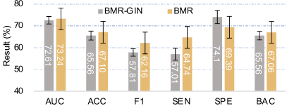
Figure 6: Results of our BMR and its variant GMR-GIN (with GIN as spatial encoder) in ASD vs. HC classification on NYU.

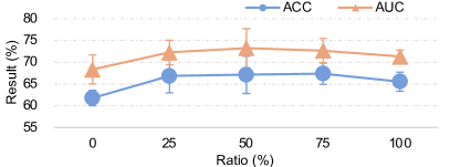
Figure 7: Results of the proposed BMR with different modularity ratios in ASD vs. HC classification on NYU.

6.4 Influence of Modularity Ratio

In the proposed modularity constraint, we randomly select $m=50\%$ of all $\frac{N_{c}(N_{c}-1)}{2}$ paired ROIs in the $c$-th module (with $N_{c}$ ROIs) to constrain the BMR. To explore the influence of modularity ratio, we vary its values within the range of $\{0\%,25\%,\cdots,100\%\}$, and report the results on NYU site of ABIDE in Fig. 7. As shown in Fig. 7, with $m<75\%$, the ACC and AUC values of BMR generally improve as the increase of $m$. With a very large modularity ratio (e.g., $m=100\%$), BMR cannot achieve satisfactory performance. The possible reason is that using a too strong modularity constraint in BMR may lead to an over-smoothing problem, thus weakening the discriminative power of learned representations.

6.5 Influence of Sliding Window Size

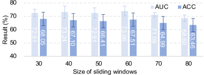
Figure 8: Results of our BMR using different sizes of sliding windows in ASD vs. HC classification on NYU.

In the main experiments, we use the sliding window strategy to generate dynamic BFNs with the window size of $\Gamma=40$. To further explore the influence of sliding window size, we vary sliding window size within $\{30,40,\cdots,80\}$ and record the results of BMR on NYU site of ABIDE in Fig. 8. As shown in Fig. 8, the BMR consistently yields promising performance (i.e., AUC $>72\%$) when the window size is within the range (i.e., $30\leq\Gamma\leq 60$). But with large size of sliding windows (e.g., $\Gamma=80$), BMR cannot achieve good performance. The reason could be that a larger window size provides lower temporal resolution, so that the BMR can not effectively capture temporal fluctuations within fMRI series.

6.6 Influence of Distance Metric

We employ the cosine distance in BMR to quantify the similarity between latent node-level representations within each module, as shown in Eq. 4. To study the effect of this metric, we compare BMR with its three variants: (1) BMR-ED with Euclidean distance, (2) BMR-HD with Hamming distance, and (3) BMR-JD with Jaccard similarity, with results reported in Table 4. As shown in Table 4, BMR using four different distance metrics in the modularity constraint achieves comparable results. This implies that our BMR is not sensitive to the distance metrics used in the modularity constraint.

Table 4: Performance of the proposed BMR and its three variants that use different similarity metrics in the proposed modularity constraint in ASD vs. HC classification on NYU.

Method	AUC (%)	ACC (%)	F1 (%)	SEN (%)	SPE (%)	PRE (%)
BMR-ED	73.00(1.69)	65.88(2.86)	60.62(3.33)	64.37(3.80)	68.19(2.51)	66.28(2.40)
BMR-HD	72.03(2.69)	64.75(2.57)	59.04(3.21)	60.88(4.21)	68.25(4.20)	64.57(2.52)
BMR-JS	73.12(3.01)	66.92(4.54)	61.48(4.85)	63.13(4.80)	70.53(6.20)	66.83(4.61)
BMR	73.24(4.48)	67.10(4.29)	62.16(4.53)	64.74(5.08)	69.39(6.22)	67.06(4.38)

6.7 Influence of BFN Sparsity Ratio

Following [24], we empirically retain the top 30% strongest edges (i.e., sparsity ratio) in each BFN in the experiments. To study the impact of sparsity ratio, we vary its value within $\{10\%,\cdots,100\%\}$ and report AUC and ACC values in ASD vs. HC classification on NYU in Fig. 9. As shown in Fig. 9, our BMR achieves stable results when sparsity ratio is $<60\%$. For example, BMR obtains the AUC values of $73.69\%$ and $73.32\%$ when sparsity ratios are set as $10\%$ and $50\%$, respectively. The reason could be that BMR retains the most reliable and informative connections in BFNs by prioritizing the strongest edges, reducing the impact of noisy or redundant connections. But when the sparsity rate is large (e.g., $>90\%$), the BMR cannot produce good results. The possible reason is that the BFN with such large sparsity can not effectively reflect topology information due to the loss of too many connections.

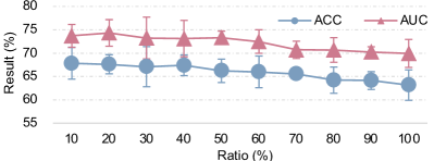
Figure 9: Results of the proposed BMR with different sparsity ratios of BFN in ASD vs. HC classification on NYU.

6.8 Limitations and Future Work

Several limitations need to be considered in future work. First, we only characterize pairwise relationships of ROIs within three prominent neurocognitive modules (i.e., SN, CEN, and DMN) as prior knowledge to design the modularity constraint in BMR. It is meaningful to design disease-specific modularity constraints based on neurocognitive research and clinical experience in the future. Second, the BMR incorporates known brain modular organization into fMRI representation learning. Future work will seek to design new algorithms that can automatically detect unknown brain modular structures during graph/BFN learning to characterize disease-induced brain changes. Besides, the BMR needs to be trained on labeled fMRI data in a supervised manner. In future work, we will employ unsupervised contrastive learning strategies [47] to pre-train the feature encoder on large-scale unlabeled data to learn more discriminative fMRI features.

7 Conclusion

In this paper, we propose a Brain Modularity-constrained dynamic Representation learning (BMR) framework for interpretable fMRI analysis. Specifically, we first construct a dynamic graph/BFN for each subject, and then design a brain modularity-constrained GNN model for dynamic graph representation learning, where a novel modularity constraint is developed to encourage nodes within the same module to share similar embeddings. We also propose a graph topology reconstruction constraint to preserve original topology information of input BFNs during representation learning. Finally, we perform brain disorder prediction and biomarker detection by analyzing disease-related functional connectivities and brain regions, aiming to provide biological evidence for clinical practice. Extensive experiments demonstrate the effectiveness of BMR in fMRI-based brain disorder detection.

References

- Arnemann et al. [2015] Arnemann, K.L., Chen, A.J.W., Novakovic-Agopian, T., Gratton, C., Nomura, E.M., D’Esposito, M., 2015. Functional brain network modularity predicts response to cognitive training after brain injury. Neurology 84, 1568–1574.
- Azevedo et al. [2022] Azevedo, T., Campbell, A., Romero-Garcia, R., Passamonti, L., Bethlehem, R.A., Lio, P., Toschi, N., 2022. A deep graph neural network architecture for modelling spatio-temporal dynamics in resting-state functional MRI data. Medical Image Analysis 79, 102471.
- Banker et al. [2021] Banker, S.M., Gu, X., Schiller, D., Foss-Feig, J.H., 2021. Hippocampal contributions to social and cognitive deficits in autism spectrum disorder. Trends in Neurosciences 44, 793–807.
- Bessadok et al. [2022] Bessadok, A., Mahjoub, M.A., Rekik, I., 2022. Graph neural networks in network neuroscience. IEEE Transactions on Pattern Analysis and Machine Intelligence .
- Biau and Scornet [2016] Biau, G., Scornet, E., 2016. A random forest guided tour. Test 25, 197–227.
- Bolt et al. [2022] Bolt, T., Nomi, J.S., Bzdok, D., Salas, J.A., Chang, C., Thomas Yeo, B., Uddin, L.Q., Keilholz, S.D., 2022. A parsimonious description of global functional brain organization in three spatiotemporal patterns. Nature Neuroscience 25, 1093–1103.
- Chen et al. [2022] Chen, H., Gomez, C., Huang, C.M., Unberath, M., 2022. Explainable medical imaging ai needs human-centered design: Guidelines and evidence from a systematic review. NPJ Digital Medicine 5, 156.
- Chen and Guestrin [2016] Chen, T., Guestrin, C., 2016. Xgboost: A scalable tree boosting system, in: Proceedings of the 22nd ACM SIGKDD International Conference on Knowledge Discovery and Data Mining, pp. 785–794.
- Chockanathan et al. [2019] Chockanathan, U., DSouza, A.M., Abidin, A.Z., Schifitto, G., Wismüller, A., 2019. Automated diagnosis of HIV-associated neurocognitive disorders using large-scale granger causality analysis of resting-state functional MRI. Computers in Biology and Medicine 106, 24–30.
- Di Martino et al. [2014] Di Martino, A., Yan, C.G., Li, Q., Denio, E., Castellanos, F.X., Alaerts, K., Anderson, J.S., Assaf, M., Bookheimer, S.Y., Dapretto, M., et al., 2014. The autism brain imaging data exchange: Towards a large-scale evaluation of the intrinsic brain architecture in autism. Molecular Psychiatry 19, 659–667.
- Dichter et al. [2009] Dichter, G.S., Felder, J.N., Bodfish, J.W., 2009. Autism is characterized by dorsal anterior cingulate hyperactivation during social target detection. Social Cognitive and Affective Neuroscience 4, 215–226.
- DSouza et al. [2019] DSouza, A.M., Abidin, A.Z., Schifitto, G., Wismüller, A., 2019. A multivoxel pattern analysis framework with mutual connectivity analysis investigating changes in resting state connectivity in patients with HIV associated neurocognitve disorder. Magnetic Resonance Imaging 62, 121–128.
- Gadgil et al. [2020] Gadgil, S., Zhao, Q., Pfefferbaum, A., Sullivan, E.V., Adeli, E., Pohl, K.M., 2020. Spatio-temporal graph convolution for resting-state fMRI analysis, in: Medical Image Computing and Computer Assisted Intervention–MICCAI 2020: 23rd International Conference, Lima, Peru, October 4–8, 2020, Proceedings, Part VII 23, Springer. pp. 528–538.
- Gallen and D’Esposito [2019] Gallen, C.L., D’Esposito, M., 2019. Brain modularity: A biomarker of intervention-related plasticity. Trends in Cognitive Sciences 23, 293–304.
- Gan et al. [2021] Gan, J., Peng, Z., Zhu, X., Hu, R., Ma, J., Wu, G., 2021. Brain functional connectivity analysis based on multi-graph fusion. Medical Image Analysis 71, 102057.
- Geirhos et al. [2020] Geirhos, R., Jacobsen, J.H., Michaelis, C., Zemel, R., Brendel, W., Bethge, M., Wichmann, F.A., 2020. Shortcut learning in deep neural networks. Nature Machine Intelligence 2, 665–673.
- Goulden et al. [2014] Goulden, N., Khusnulina, A., Davis, N.J., Bracewell, R.M., Bokde, A.L., McNulty, J.P., Mullins, P.G., 2014. The salience network is responsible for switching between the default mode network and the central executive network: Replication from DCM. NeuroImage 99, 180–190.
- He et al. [2009] He, Y., Wang, J., Wang, L., Chen, Z.J., Yan, C., Yang, H., Tang, H., Zhu, C., Gong, Q., Zang, Y., et al., 2009. Uncovering intrinsic modular organization of spontaneous brain activity in humans. PloS One 4, e5226.
- Hu et al. [2018] Hu, J., Shen, L., Sun, G., 2018. Squeeze-and-excitation networks, in: Proceedings of the IEEE Conference on Computer Vision and Pattern Recognition, pp. 7132–7141.
- Hu et al. [2022] Hu, R., Peng, L., Gan, J., Shi, X., Zhu, X., 2022. Complementary graph representation learning for functional neuroimaging identification, in: Proceedings of the 30th ACM International Conference on Multimedia, pp. 3385–3393.
- Jiang et al. [2020] Jiang, H., Cao, P., Xu, M., Yang, J., Zaiane, O., 2020. Hi-GCN: A hierarchical graph convolution network for graph embedding learning of brain network and brain disorders prediction. Computers in Biology and Medicine 127, 104096.
- Khosla et al. [2019] Khosla, M., Jamison, K., Ngo, G.H., Kuceyeski, A., Sabuncu, M.R., 2019. Machine learning in resting-state fMRI analysis. Magnetic Resonance Imaging 64, 101–121.
- Kim and Ye [2020] Kim, B.H., Ye, J.C., 2020. Understanding graph isomorphism network for rs-fMRI functional connectivity analysis. Frontiers in Neuroscience , 630.
- Kim et al. [2021] Kim, B.H., Ye, J.C., Kim, J.J., 2021. Learning dynamic graph representation of brain connectome with spatio-temporal attention. Advances in Neural Information Processing Systems 34, 4314–4327.
- Kipf and Welling [2016a] Kipf, T.N., Welling, M., 2016a. Semi-supervised classification with graph convolutional networks. arXiv preprint arXiv:1609.02907 .
- Kipf and Welling [2016b] Kipf, T.N., Welling, M., 2016b. Variational graph auto-encoders. arXiv preprint arXiv:1611.07308 .
- Kong et al. [2021] Kong, Y., Gao, S., Yue, Y., Hou, Z., Shu, H., Xie, C., Zhang, Z., Yuan, Y., 2021. Spatio-temporal graph convolutional network for diagnosis and treatment response prediction of major depressive disorder from functional connectivity. Human Brain Mapping 42, 3922–3933.
- Krishnadas et al. [2014] Krishnadas, R., Ryali, S., Chen, T., Uddin, L., Supekar, K., Palaniyappan, L., Menon, V., 2014. Resting state functional hyperconnectivity within a triple network model in paranoid schizophrenia. The Lancet 383, S65.
- Ktena et al. [2018] Ktena, S.I., Parisot, S., Ferrante, E., Rajchl, M., Lee, M., Glocker, B., Rueckert, D., 2018. Metric learning with spectral graph convolutions on brain connectivity networks. NeuroImage 169, 431–442.
- Kunda et al. [2022] Kunda, M., Zhou, S., Gong, G., Lu, H., 2022. Improving multi-site autism classification via site-dependence minimization and second-order functional connectivity. IEEE Transactions on Medical Imaging 42, 55–65.
- Li et al. [2021] Li, X., Zhou, Y., Dvornek, N., Zhang, M., Gao, S., Zhuang, J., Scheinost, D., Staib, L.H., Ventola, P., Duncan, J.S., 2021. BrainGNN: Interpretable brain graph neural network for fMRI analysis. Medical Image Analysis 74, 102233.
- Menon and Krishnamurthy [2019] Menon, S.S., Krishnamurthy, K., 2019. A comparison of static and dynamic functional connectivities for identifying subjects and biological sex using intrinsic individual brain connectivity. Scientific Reports 9, 1–11.
- Menon [2011] Menon, V., 2011. Large-scale brain networks and psychopathology: A unifying triple network model. Trends in Cognitive Sciences 15, 483–506.
- Meunier et al. [2009] Meunier, D., Achard, S., Morcom, A., Bullmore, E., 2009. Age-related changes in modular organization of human brain functional networks. NeuroImage 44, 715–723.
- Meunier et al. [2010] Meunier, D., Lambiotte, R., Bullmore, E.T., 2010. Modular and hierarchically modular organization of brain networks. Frontiers in Neuroscience 4, 200.
- Monk et al. [2009] Monk, C.S., Peltier, S.J., Wiggins, J.L., Weng, S.J., Carrasco, M., Risi, S., Lord, C., 2009. Abnormalities of intrinsic functional connectivity in autism spectrum disorders. NeuroImage 47, 764–772.
- Murtagh [1991] Murtagh, F., 1991. Multilayer perceptrons for classification and regression. Neurocomputing 2, 183–197.
- Nebel et al. [2022] Nebel, M.B., Lidstone, D.E., Wang, L., Benkeser, D., Mostofsky, S.H., Risk, B.B., 2022. Accounting for motion in resting-state fMRI: What part of the spectrum are we characterizing in autism spectrum disorder? NeuroImage 257, 119296.
- Noble [2006] Noble, W.S., 2006. What is a support vector machine? Nature Biotechnology 24, 1565–1567.
- Pervaiz et al. [2022] Pervaiz, U., Vidaurre, D., Gohil, C., Smith, S.M., Woolrich, M.W., 2022. Multi-dynamic modelling reveals strongly time-varying resting fMRI correlations. Medical Image Analysis 77, 102366.
- Rosa et al. [2015] Rosa, M.J., Portugal, L., Hahn, T., Fallgatter, A.J., Garrido, M.I., Shawe-Taylor, J., Mourao-Miranda, J., 2015. Sparse network-based models for patient classification using fMRI. NeuroImage 105, 493–506.
- Schober et al. [2018] Schober, P., Boer, C., Schwarte, L.A., 2018. Correlation coefficients: Appropriate use and interpretation. Anesthesia & Analgesia 126, 1763–1768.
- Shin et al. [2017] Shin, N.Y., Hong, J., Choi, J.Y., Lee, S.K., Lim, S.M., Yoon, U., 2017. Retrosplenial cortical thinning as a possible major contributor for cognitive impairment in HIV patients. European Radiology 27, 4721–4729.
- Sip et al. [2023] Sip, V., Hashemi, M., Dickscheid, T., Amunts, K., Petkoski, S., Jirsa, V., 2023. Characterization of regional differences in resting-state fMRI with a data-driven network model of brain dynamics. Science Advances 9, eabq7547.
- Sporns and Betzel [2016] Sporns, O., Betzel, R.F., 2016. Modular brain networks. Annual Review of Psychology 67, 613–640.
- Velivcković et al. [2017] Velivcković, P., Cucurull, G., Casanova, A., Romero, A., Lio, P., Bengio, Y., 2017. Graph attention networks. arXiv preprint arXiv:1710.10903 .
- Wang and Qi [2022] Wang, X., Qi, G.J., 2022. Contrastive learning with stronger augmentations. IEEE Transactions on Pattern Analysis and Machine Intelligence .
- Wee et al. [2012] Wee, C.Y., Yap, P.T., Zhang, D., Wang, L., Shen, D., 2012. Constrained sparse functional connectivity networks for MCI classification, in: Medical Image Computing and Computer-Assisted Intervention–MICCAI 2012: 15th International Conference, Nice, France, October 1-5, 2012, Proceedings, Part II 15, Springer. pp. 212–219.
- Yan and Zang [2010] Yan, C., Zang, Y., 2010. DPARSF: A MATLAB toolbox for “pipeline” data analysis of resting-state fMRI. Frontiers in Systems Neuroscience 4, 13.
- Yin et al. [2022] Yin, W., Li, L., Wu, F.X., 2022. Deep learning for brain disorder diagnosis based on fMRI images. Neurocomputing 469, 332–345.
- Zhan et al. [2022] Zhan, Y., Yu, Q., Cai, D.C., Ford, J.C., Shi, X., Fellows, A.M., Clavier, O.H., Soli, S.D., Fan, M., Lu, H., et al., 2022. The resting state central auditory network: A potential marker of HIV-related central nervous system alterations. Ear and Hearing 43, 1222.
- Zhou et al. [2017] Zhou, Y., Li, R., Wang, X., Miao, H., Wei, Y., Ali, R., Qiu, B., Li, H., 2017. Motor-related brain abnormalities in HIV-infected patients: A multimodal MRI study. Neuroradiology 59, 1133–1142.