SuperBench: A Super-Resolution Benchmark Dataset for Scientific Machine Learning

Abstract

Super-Resolution (SR) techniques aim to enhance data resolution, enabling the retrieval of finer details, and improving the overall quality and fidelity of the data representation. There is growing interest in applying SR methods to complex spatiotemporal systems within the Scientific Machine Learning (SciML) community, with the hope of accelerating numerical simulations and/or improving forecasts in weather, climate, and related areas. However, the lack of standardized benchmark datasets for comparing and validating SR methods hinders progress and adoption in SciML. To address this, we introduce SuperBench, the first benchmark dataset featuring high-resolution datasets (up to $2048\times 2048$ dimensions), including data from fluid flows, cosmology, and weather. Here, we focus on validating spatial SR performance from data-centric and physics-preserved perspectives, as well as assessing robustness to data degradation tasks. While deep learning-based SR methods (developed in the computer vision community) excel on certain tasks, despite relatively limited prior physics information, we identify limitations of these methods in accurately capturing intricate fine-scale features and preserving fundamental physical properties and constraints in scientific data. These shortcomings highlight the importance and subtlety of incorporating domain knowledge into ML models. We anticipate that SuperBench will significantly advance SR methods for scientific tasks.

1 Introduction

Super-Resolution (SR) techniques have emerged as powerful tools for enhancing data resolution, improving the overall quality and fidelity of data representation, and retrieving fine-scale structures. These techniques find application in diverse fields such as image restoration and enhancement [52, 70, 67, 50], medical imaging [25, 28], astronomical imaging [54, 36], remote sensing [7], and forensics [60]. Despite the remarkable achievements of deep learning-based SR methods developed primarily in the computer vision community [5, 70], their application to scientific tasks has certain limitations. In particular, these methods, state-of-the-art (SOTA) within machine learning (ML), often struggle to capture intricate fine-scale features accurately and to preserve fundamental physical properties and constraints inherent in scientific data. These shortcomings highlight the challenge of incorporating domain knowledge into ML models. While these are well-known anecdotal observations (that we confirm), a more basic issue is that the progress and widespread adoption of SR methods in the scientific and scientific machine learning (SciML) communities face a significant challenge: the absence of standardized benchmark datasets for comparing and validating the performance of different SR approaches. To address this crucial gap, we introduce SuperBench, an innovative benchmark dataset that fills the need for standardized evaluation and comparison of SR methods within scientific domains.

Problem setup.  SR is a task that involves recovering fine-scale data from corresponding coarse-grained data. In the context of scientific SR, let us consider the example of weather data that captures complex interactions among the atmosphere, oceans, and land surface, illustrated in Figure 1. The coarse-grained data can be regarded as a down-sampled version of the fine-scale data. The former coarse-scale data can be represented as low-dimensional data $x\in\mathcal{X}$; while the latter fine-scale data can be seen as high-dimensional data $y\in\mathcal{Y}$.

In practice, there are various degradation functions $f$ that can generate the coarse-grained data. We can model the degradation process as $x=f(y)+\epsilon$, where $f:\mathcal{Y}\rightarrow\mathcal{X}$ is a degradation function, and $\epsilon$ represents noise. The degradation function $f$ can be non-linear, and the noise term $\epsilon$ can have complex spatial and temporal patterns. For example, a simple degradation function commonly used is bicubic down-sampling [5, 70]. However, this simplistic approach does not capture the challenges of real-world SR problems [11, 45], where more complex unknown degradations are typically encountered. Thus, we also consider more realistic degradations such as uniform down-sampling with noise, to simulate experimental measurement setups, and direct low-resolution (LR) simulations of data, which also pose significant challenges for SR techniques. SR works in the opposite direction of down-sampling, aiming to recover an high-resolution (HR) representation (including fine-scale structures) from the given coarse-grained data $x$. More concretely, the aim is to find an inverse map $f^{-1}:\mathcal{X}\rightarrow\mathcal{Y}$ that accurately restores the fine-scale details. Of course, SR is difficult due to the complex fine-scale structures in the high-dimensional data, which cannot be fully described by the limited information present in the low-dimensional data. This inverse problem often has multiple solutions, especially when dealing with higher up-sampling factors from the low-dimensional to high-dimensional space.

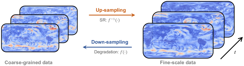
Figure 1: High-resolution data are paramount to accurately resolving the turbulent dynamics of Earth’s weather systems. For instance, resolving storms requires kilometer-scale resolutions, and some crucial climate processes can require order of 1m resolutions. The snapshots on the left show coarse-grained data that can be thought of as a down-sampled representation of the fine-scale data on the right. Coarse-grained data not only fail to capture the small scales, but they also do not account for the impact of these small scales on the large-scale dynamics, nor the impact of fine (and critical) topographic features such as mountain ranges on either scale. Today, generating these high-resolution and accurate data demand prohibitive computational resources (thousands of nodes on modern super-computing substrates). Based on current computing trends, it may be several decades before numerical solvers of atmospheric physics can simulate at a meter resolution [61], which represents a grand challenge to scientific computing. Using SR to resolve fine-scale structures from coarser simulations holds an enormous promise towards fast, efficient, and accurate models for atmospheric physics emulation.

In this paper, we are concerned with establishing a HR benchmark dataset, SuperBench, for spatial SR methods for scientific problems. By providing a standardized benchmark dataset, SuperBench empowers SciML researchers to evaluate and advance SR methods specifically tailored for scientific tasks. We anticipate that this benchmark dataset will significantly contribute to the advancement of SR techniques in scientific domains, enabling the development of more effective and reliable methods for enhancing data resolution and improving scientific insights.

Main contributions.  The key contributions of this paper are summarized as follows.

• We introduce SuperBench (https://github.com/erichson/SuperBench), a novel benchmark dataset comprising high-quality scientific data for spatial SR methods. This dataset includes four distinct datasets of HR simulations, with dimensions up to $2048\times 2048$, surpassing the resolution of typical scientific datasets used in SciML. SuperBench has a file size of 268GB in total. The datasets feature challenging problems in fluid flows, cosmology, and climate science. These datasets are specifically chosen to push the performance limits of existing methods and facilitate the development of innovative SR methods for scientific applications.

• We investigate a range of degradation functions tailored for scientific data. In addition to commonly used methods like uniform and bicubic downscaling, we explore the use of LR simulations as inputs and consider the introduction of noise to the input data. This suits SuperBench for a thorough assessment and effective comparison of different SR methods.

• We benchmark existing SR methods on SuperBench. By employing both data and physical-centric metrics, our analysis provides valuable insights into the performance of various SR approaches. Notably, our findings demonstrate that purely data-driven SR methods, even those employing advanced architectures like Transformers, struggle to preserve the physical properties of turbulence datasets. An illustrative example of the performance of baseline models on weather data is shown in Figure 2, which shows the limitations of current approaches for modeling multi-scale structures.

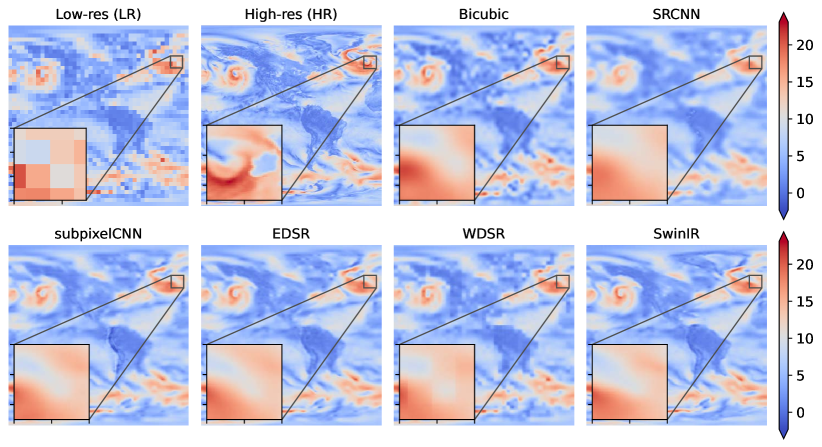
Figure 2: A cropped example snapshot of weather data. The task is to recover the HR representation from the corresponding LR input by a factor of $\times 16$. All SOTA methods reconstruct a blurred approximation that washes out important multi-scale and fine-scale features.

The motivation behind creating a SR benchmark dataset for scientific problems stems from two key factors: (i) the prohibitively high computational cost associated with executing HR numerical simulations; and (ii) the inherent limitations of measurements in large-scale experiments, which often have restricted resolution. It is important to note that SR applied to scientific data differs from its application to general image data in two significant ways. Firstly, many physical systems adhere to explicit governing laws and exhibit distinct features at fine scales, such as multi-scale turbulence phenomena. Thus, preserving the inherent physical properties of scientific data during the SR process becomes a crucial objective. As a potential research direction, exploring constrained ML methods, including soft versus hard constraints and equality versus inequality constraints, could prove fruitful here [34, 16, 51]. Secondly, the evaluation metrics for SR on scientific data may differ, as scientists are primarily concerned with pixel-wise reconstruction accuracy and specific domain-dependent metrics. For these and other reasons, assessing the performance of SR methods necessitates a high-quality scientific benchmark dataset.

Limitations. We limit the scope of this benchmark dataset to spatial SR tasks, which still pose a range of challenges for existing SR methodology in the context of scientific applications. However, there is an increasing interest in applying SR methods to dynamic system applications (e.g., videos or fluid flows) where the model aims to recover temporal or both spatial and temporal information.

2 Related Work

A wide range of methods exist for SR [50]. However, it has been well-established that deep learning offers a powerful and versatile framework for SR solutions, as demonstrated in [5], [75], and the references therein. Moreover, recent studies have shown the effectiveness of deep learning-based SR methods specifically for fluid flows [20, 39, 17, 8, 22]. In the following, we provide a brief overview of the most notable deep learning-based SR methods that are relevant to our benchmark dataset.

Single-image SR methods.  Single-image SR (SISR) focuses on tackling spatial SR. SRCNN [14] is the first iconic work of introducing deep convolutional neural networks (CNNs) for SISR; and it drastically improves the reconstruction performance, compared with the traditional method based on sparse representation [80]. In addition to the interpolation-based up-sampling used in SRCNN, the strategies of deconvolution [15] and pixelshuffle [62] also attract considerable critical attention. Furthermore, due to a proliferation of network designs, we observe increasingly rapid advances in the field of SISR. Generally, there are six model architectures: residual networks [31, 38, 82]; recursive blocks [64]; dense networks [69, 86]; generative adversarial networks (GAN) [35, 74, 85, 12]; attention schemes [78, 13, 37]; and diffusion models [58, 59].

Constrained SR.  Recently, researchers have shown great interest in SR of scientific data (e.g., fluid flow). For example, neural networks have been introduced to reconstruct fluid flows by learning an end-to-end mapping between LR data and HR solution field based on either limited sensor measurements [17] or sufficient labeled simulations [77, 83, 20, 39, 21, 23, 71, 22]. Moreover, many scientists start to explore the potential of incorporating domain-specific constraints into the learning process, due to the accessibility of physical principles. In the context of scientific tasks, the realm of constrained SR has been investigated in two primary directions. The first direction involves the integration of constraints into the loss function, which guides the optimization process. In specific, the popular physics-informed neural networks (PINNs) [55, 30, 34, 16] are essentially constructed in a soft-constraint strategy. Due to the simplicity of this penalty method, there have been various downstream applications of physics-informed SR for scientific data [72, 63, 24, 18, 57, 10].

Related benchmarks.  In recent years, a number of benchmarks and datasets have been developed to facilitate the evaluation and comparison of SR methods. Among them, several prominent benchmarks have gained wide recognition as standardized evaluation datasets for both traditional and deep learning-based SR methods, such as Train91 [79], Set5 [9], Set14 [84], B100 [48], Urban100 [27], and 2K resolution high-quality DIV2K [2]. Moreover, the bicubic down-sampling is the most commonly employed degradation operator to simulate the transformation from HR to LR images.

In addition, there exist specialized benchmarks and datasets that are available for scientific domains. They aim to tackle distinct challenges and specific requirements of scientific applications. For instance, one scientific benchmark [66] covers diverse scientific problems. PDEBench [65] serves as a benchmark suite for the simulation tasks of a wide range of Partial Differential Equations (PDEs). A novel domain-specific dataset, SustainBench [81], is provided for development economics and environmental science. Furthermore, the open-source library DeepXDE [44] offers comprehensive scientific ML solutions, particularly focusing on PINN [55] and DeepONet [43] methods.

3 Description of SuperBench

SuperBench serves as a benchmark dataset for evaluating spatial SR methods in scientific applications. It aims to achieve two primary objectives: (1) expand the currently available SR datasets, particularly by incorporating HR datasets with dimensions such as $2048\times 2048$ and beyond; and (2) enhance the diversity of data by extending the scope of SR to scientific domains. To achieve these goals, we specifically focus on fluid flows, cosmology, and weather data. These data exhibit multi-scale structures that present challenging problems for SR methods. Examples are shown in Figure 3.

3.1 Datasets

Table 1 presents a brief summary of the datasets included in SuperBench. The benchmark dataset comprises four different datasets, from three different scientific domains. Among them are two fluid flow datasets, featuring varying Reynolds numbers ($Re$) to capture different flow regimes. Additionally, SuperBench encompasses a cosmology dataset and a weather dataset, ensuring a diverse range of scientific contexts for evaluating SR methods. To facilitate training without the need for multi-GPU computing, the spatial resolution of the datasets is carefully chosen. This consideration ensures that users can effectively use the benchmark dataset without encountering computational constraints during training and inference. Details of each dataset are provided in the subsequent sections.

\begin{overpic}[width=433.62pt]{figs/nskt_snapshot_intro.pdf} \end{overpic}

\begin{overpic}[width=433.62pt]{figs/climate_snapshot_intro.pdf} \end{overpic}

\begin{overpic}[width=433.62pt]{figs/cosmo_snapshot_intro.pdf} \end{overpic}

Figure 3: High-resolution example snapshots included in SuperBench, showing a Navier-Stokes Kraichnan Turbulence fluid flow (left), weather data that are comprised of several atmospheric variables (middle), and simulated cosmology hydrodynamics data (right).

Table 1: Summary of datasets in SuperBench.

Datasets	Spatial resolution	# samples (train/valid/test)	File size
Fluid flow data ($Re=16000$)	$1024\times 1024$	1200 / 200 / 400	57GB
Fluid flow data ($Re=32000$)	$1024\times 1024$	1200 / 200 / 400	57GB
Cosmology data	$2048\times 2048$	1200 / 200 / 400	76GB
$\quad\hookrightarrow$ (w/ LR sim.)	$2048\times 2048$	800 / 100 / 100	39GB
Weather data	$720\times 1440$	1460 / 365 / 730	39GB

3.1.1 Navier-Stokes Kraichnan Turbulence (NSKT) Fluid Flows

Fluid flows are ubiquitous in diverse scientific, engineering, and technological domains, including environmental science, material sciences, geophysics, astrophysics, and chemical engineering; and the understanding and analysis of fluid flows have significant implications across these disciplines. In particular, turbulence is a chaotic phenomenon that arises within fluid flows. While the Navier-Stokes (NS) equations serve as a fundamental framework for elucidating fluid motion, their solution becomes increasingly arduous and challenging in the presence of turbulence. The NS equations that couple the velocity field to pressure gradients are given by

$$\nabla\cdot\mathbf{u}=0,\quad\frac{\partial\mathbf{u}}{\partial t}+\mathbf{u}\cdot\nabla\mathbf{u}=-\frac{1}{\rho}\nabla\mathbf{p}+\nu\nabla^{2}\mathbf{u},$$ (1)

where $\mathbf{u}$ is the velocity field and $\mathbf{p}$ is the pressure. Moreover, $\rho$ and $\nu$ denote the density and the viscosity, respectively. The Kraichnan model provides a simplified approach to studying turbulent and chaotic behavior in fluids. In this work, we consider two-dimensional Kraichnan turbulence in a doubly periodic square domain within $[0,2\pi]^{2}$ [53]. The spatial domain is discretized using $2048^{2}$ degrees of freedom (DoF), and the solution variables of NS equations are obtained from direct numerical simulation (DNS). A second-order energy-conserving Arakawa scheme [6] is employed for computing the nonlinear Jacobian, and a second-order finite-difference scheme is used for the Laplacian of the vorticity.

Data. We provide two fluid flow datasets that are simulated with Reynolds numbers of $Re=16000$ and $Re=32000$. These original simulations are based on spatial grids with a resolution of $2048\times 2048$. To facilitate the training and validation processes, we carefully select a sub-region from these grids, precisely $1024\times 1024$, which corresponds to a specific sub-domain defined as $[0,\pi]^{2}$. For testing purposes, we employ another sub-domain $[\pi,2\pi]^{2}$ within the same spatial resolution. Both the LR inputs and the HR counterparts consist of three channels, each of which represents a distinct physical quantity. Specifically, these channels denote two velocity variables in the $x$ and $y$ directions, as well as with the vorticity field.

3.1.2 Cosmology Hydrodynamics

The large-scale structure of the universe is shaped by the parameters of a given cosmological model, as well as by initial conditions. By comparing observational maps of some traces of matter like galaxies or the Lyman $\alpha$ forest (see, e.g., [42, 1]) against high-fidelity simulated model universes (see, e.g., [46, 47]), we can constrain the parameters of our cosmological model, such as the nature of dark matter and dark energy, the history of inflation, the reionization in the early universe, or the mass of neutrino particles [4]. In this work, we will use simulation data from Nyx, a massively parallel multiphysics code, developed for simulations of the Lyman $\alpha$ forest. The Nyx code [3] follows the evolution of dark matter modeled as self-gravitating Lagrangian particles, while baryons are modeled as an ideal gas on a set of rectangular Cartesian grids. Besides solving for gravity and the Euler equations, the code also includes the physical processes relevant for the accurate representation of the Ly$\alpha$ forest: chemistry of the gas in the primordial composition of hydrogen and helium, inverse Compton cooling off the microwave background, while keeping track of the net loss of thermal energy resulting from atomic collisional processes [46]. All cells are assumed to be optically thin to ionizing radiation, and radiative feedback is accounted for via a spatially uniform, time-varying ultra-violet background radiation. The intricate interactions among diverse physical processes in cosmology data give rise to highly complex multi-scale features, which pose challenges for SR methods.

Data. We generate two independent pairs of LR and HR simulations with $512^{3}$ and $4096^{3}$ resolution elements, respectively. LR and HR simulations in each pair start from the identical initial conditions, and the pairs differ in the random realiztion but share the same physical and cosmological parameters. Both datasets comprise temperature and baryon density variables.

The 2D HR slices are obtained by extracting a fixed sub-domain from the original simulations with a spatial resolution of $2048\times 2048$ along the $x$-axis. Note that the training/validation and testing datasets are from two independent pairs of simulations. The first dataset aims to test the degradation methods of uniform/bicubic down-sampling. Additionally, we offer a cosmology dataset that uses LR simulation data as inputs to evaluate spatial SR methods in practical applications. The LR simulation is generated with a $512^{3}$ grid, and the LR counterparts in SuperBench are selected from the corresponding LR sub-region, with a spatial resolution of $256^{2}$. This dataset serves as a specific data degradation method in the field of SR, which imitates real-world simulation scenarios. It is noteworthy that the temperature and baryon density in SuperBench are presented in the logarithmic space due to their significant magnitudes.

3.1.3 Weather

Global weather spatiotemporal patterns exhibit highly complex interactions between several physical processes that include turbulence, multi-scale fluid flows, radiation/heat transfer, and multi-phase chemical and biological physics across the atmosphere, ocean, and land surfaces. These interactions span a wide range of spatial and temporal scales that extend over $\mathcal{O}(10)$ orders of magnitude. For instance, spatial scales can span from micrometers (highly localized fluid physics) to thousands of kilometers (full planetary scales). In this work, we consider ERA5 [26] (downloaded from the Copernicus Climate Change Service (C3S) Climate Data Store), a publicly available dataset from the European Centre for Medium-Range Weather Forecasts (ECMWF). It comprises hourly estimations of multiple atmospheric variables and covers the region from the Earth’s surface up to an altitude of approximately 100 km (discretized at 37 vertical levels) with a spatial resolution of $0.25^{\circ}$ (25 km) (in latitude and longitude). When represented on a cartesian grid, these variables are a 720 $\times$ 1440 pixel field at any given altitude. ERA5 encompasses a substantial temporal scope, spanning from the year 1979 to the present day, and it is generated by assimilating observations from diverse measurement sources with a SOTA numerical model (solver) using a Bayesian estimation process [29]. It represents an optimal reconstruction of the observed history of the earth’s atmospheric state.

Data.  We provide one dataset that is a subset of ERA5 and consists of three channels for conducting the SR experiments: Kinetic Energy (KE) at 10m from the surface, defined as $\sqrt{u^{2}+v^{2}}$, where $u$ and $v$ are the wind velocity components at 10m altitude; the temperature at 2m from surface; and total column water vapor. These three quantities represent different and crucial prognostic variables—wind velocities are critical for wind and energy resource planning and typically need high resolutions to forecast accurately; surface temperatures are widely tracked during extreme events such as heat waves and for climate change signals; and total column water vapor is diagnostic of precipitation that usually manifests small scale features. The variables are sampled at a frequency of 24 hours (at 00:00 UTC everyday) for 7 years.

3.2 Data Preprocessing

It should be noted that the range of the scientific data provided by SuperBench is not limited to the common interval of $[0,255]$, which is typically associated with image data in computer vision. Rather, within the SuperBench dataset, we encounter a broad range of data magnitudes, and this presents challenges when assessing baseline performance. To overcome this challenge and ensure a fair evaluation, we standardize the input and target data, using the mean and standard deviation specific to the dataset being evaluated. By normalizing the data, we bring it within a consistent range, allowing for a standardized assessment of baseline performance. Consequently, the evaluation results accurately reflect the relative performance of the baseline methods on the normalized data, ensuring a reliable and robust assessment. In addition, detailed information regarding the preprocessing of datasets and the creation of interpolation and extrapolation validation/test sets can be found in Appendix A.

4 Evaluation Metrics

In our study, we evaluate a range of SOTA SR methods (see below) to establish a solid baseline for the presented problems. To assess the performance of these methods, we employ three distinct types of metrics: pixel-level difference metrics; human-level perception metrics; and domain-motivated error metrics.

The pixel-level difference metrics enable us to evaluate quantitatively the SR algorithms by measuring the disparities between the HR ground truth and the generated super-resolved images. These metrics, such as mean squared error (MSE), peak signal-to-noise ratio (PSNR), and structural similarity index (SSIM), provide objective assessments of the fidelity and accuracy of the reconstructed details. By leveraging these metrics, we gain valuable insights into the overall quality of the SR methods’ reconstructions. The human-level perception metrics permit us to go beyond solely relying on pixel-level metrics that may not capture the perceptual quality of the super-resolved images, as human perception often differs from pixel-wise differences. In particular, by considering human perception, we can evaluate the SR methods based on their ability to produce visually pleasing results that align with human expectations. Finally, we recognize the importance of domain-specific evaluations in scientific applications. Hence, we use domain-motivated error metrics that are tailored to the specific requirements and constraints of the scientific domains under consideration. Incorporating such domain-specific metrics allows us to assess the suitability and effectiveness of SR methods for scientific research purposes.

While our evaluation framework includes standardized metrics that provide a holistic understanding of SR method performance for scientific applications, clearly researchers may have unique research questions and requirements that call for the use of custom metrics. To facilitate such scenarios, our SuperBench framework offers a user-friendly interface for defining and incorporating custom evaluation metrics. This flexibility empowers researchers to tailor the evaluation process to their specific needs and explore novel metrics that address the nuances of their research questions.

Pixel-level difference.  To assess the pixel-level differences between the predicted HR data $\hat{y}$ and the ground truth data $y$, we employ two key metrics: the relative Frobenius norm error (RFNE) and the Peak signal-to-noise ratio (PSNR). These metrics are defined as

$$\text{RFNE}(y,\hat{y})=\frac{\|y-\hat{y}\|_{\text{F}}}{\|y\|_{\text{F}}}\times 100\%,\quad\text{and}\quad\text{PSNR}(y,\hat{y})=10\cdot\log_{10}\frac{{\text{max}}(y)}{\text{MSE}(y,\hat{y})},$$ (2)

where $\|\cdot\|_{\text{F}}$ denotes the Frobenius norm, MSE($\cdot$) is the mean-squared error, and max($\cdot$) denotes the maximum value. By quantifying the differences between the predicted and ground truth data, these metrics enable a comprehensive assessment of the pixel-level fidelity achieved by the SR algorithms. They provide valuable information for evaluating the accuracy and effectiveness of SR methods, and they are relevant for applications that demand high precision in pixel-wise reconstruction. In addition, we also consider the infinity norm as a metric to assess extreme statistical properties.

Human-level perception.  The impact of minor perturbations and content shifts on the signal $y$ can lead to substantial degradation in both RFNE and PSNR, even when the underlying content or patterns remain unchanged [2]. Hence, there is a growing interest in evaluating SR algorithms in a structural manner that aligns with human perception. To this end, the structural similarity index measure (SSIM) [76, 75] can be used as a metric for evaluating SR algorithms. SSIM is a perception-based metric that focuses on image and graphical applications. In contrast to metrics like RFNE and PSNR, which primarily measure the pixel-wise discrepancies between the super-resolved data and their ground truth counterparts, SSIM takes into account the structural information and relationships within the images. By considering the structural characteristics of the data, SSIM provides a more nuanced evaluation of the SR algorithms, capturing perceptual similarities that go beyond pixel-level differences. In turn, a more comprehensive understanding of the performance of SR algorithms in real-world scenarios is obtained.

Domain-motivated error metrics.  Within our SuperBench framework, we provide researchers with the flexibility to incorporate domain-motivated error metrics. This is particularly valuable in scientific domains where prior knowledge is available. These metrics allow for a more comprehensive evaluation of SR methods by considering domain-specific constraints and requirements. In scientific domains such as fluid dynamics, where the preservation of continuity and conservation laws is crucial, it becomes essential to assess the SR algorithms from such a physical perspective [73, 18]. Researchers can incorporate evaluation metrics that focus on physical aspects and examine the reconstructed variables to ensure they adhere to these fundamental principles. By integrating such domain-specific metrics, a more accurate assessment of the SR algorithms can be achieved, enhancing their applicability and reliability in scientific research. In this paper, we provide a physics error metric that evaluates the preservation of continuity property in fluid flow datasets [73]. Similarly, in climate science, the evaluation metrics often involve multi-scale analysis due to the presence of multi-scale phenomena that are ubiquitous in this field. Researchers may employ metrics such as the Anomaly Correlation Coefficient (ACC) [56] to evaluate the performance of SR methods. These metrics enable the assessment of how well the SR algorithms capture and represent the complex, multi-scale features present in climate data. By considering the multi-scale aspects and incorporating relevant metrics, researchers can gain a deeper understanding of the effectiveness of SR methods in addressing the challenges posed by climate science applications.

5 Experiments and Analysis

This section presents our experimental setup and performance analysis of baseline models using the SuperBench datasets. The aim of SuperBench is to provide more challenging and realistic SR settings, considering the remarkable progress achieved in SISR research [49]. To accomplish this goal, we incorporate various data degradation schemes within the SuperBench framework. These schemes simulate realistic degradation scenarios encountered in scientific applications. Specifically, we consider the following baseline models: Bicubic interpolation; SRCNN [14]; Sub-pixel CNN [62]; EDSR [38]; WDSR [82]; and SwinIR [37]. See Appendix B and C for detailed information regarding the baseline models and the corresponding training protocol.

5.1 Evaluation Setup

In SuperBench, we define three distinct data degradation scenarios for spatial SR tasks, each designed to model a specific scientific situation: (i) The general CV scenario, which involves bicubic down-sampling. This scenario serves as a standard degradation method for SR evaluation in various image processing applications. (ii) The uniform down-sampling scenario, which considers noise in addition to down-sampling, mimicking the experimental measurement process encountered in scientific domains. This scenario aims to replicate the challenges of accurately reconstructing data from low-fidelity measurements obtained by experimental sensors. (iii) The direct use of LR simulation data as inputs, which is specific to scientific modeling. This scenario explores the performance of SR algorithms when provided with LR data generated through simulation processes. (We should note that there is a large space of possibilities here, e.g., involving sophisticated spatial and/or temporal coarse-graining of simulations, most of which we will not address here.)

Up-sampling factors.  For scenarios (i) and (ii), SuperBench offers two tracks of up-sampling factors: $\times 8$ and $\times 16$. These factors determine the level of up-sampling required to recover the HR details from the degraded LR inputs. We consider a scaling factor of $\times$16, motivated by the growing interest in significant up-sampling factors for scientific SR [24]. For scenario (iii), we specifically test the $\times 8$ up-sampling on the cosmology dataset using LR simulation data with a spatial resolution of $256\times 256$ as inputs. The HR counterparts in this scenario have an exceptionally high resolution of $2048\times 2048$, representing the challenges associated with SR tasks in the cosmology domain.

Data noise.  Recognizing the presence of noise in scientific problems, we provide the option to evaluate the performance of the SuperBench dataset under noisy LR scenarios, specifically in scenario (ii). This feature aligns with the scientific requirement for accurate data reconstruction from low-fidelity measurements obtained by experimental sensors, ensuring a faithful representation of the underlying physical phenomena. The noise level in the dataset is defined by the channel-wise standard deviation of the specific dataset. Additionally, users have the flexibility to define custom noise ratios of interest. In our SuperBench experiments, we test cases with noise levels set at $5\%$ and $10\%$ to assess the robustness and performance of SR methods under different noise conditions.

5.2 Results

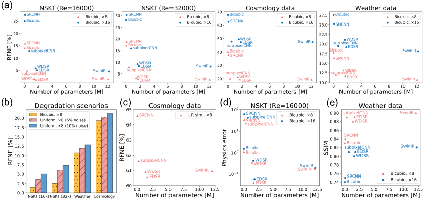
Figure 4: A summary of the baseline performance. (a) The results of RFNE versus model parameters on four datasets considering scenario (i) with up-sampling factors $\times 8$ and $\times 16$. (b) A comparative result of different degradation methods. (c) The results of scenario (iii) with LR simulation data as inputs. (d) The result of testing physics loss. (e) The evaluation of multi-scale features.

General performance.  As shown in Figure 4(a), the baseline SR methods achieve good pixel-level accuracy for super-resolving the fluid flow datasets, but they fail to perform well on both cosmology and weather data. This discrepancy arises from the more complex multi-scale structures and variations present in cosmology and weather data. Figure 4(b) also presents the difficulty of each dataset, where the cosmology data is the most challenging. Moreover, SwinIR achieves the SOTA performance on SuperBench, outperforming residual networks (EDSR and WDSR).

Up-sampling factors.  Figure 4(a) illustrates significant RFNE discrepancies between the two up-sampling factors ($\times 8$ and $\times 16$) across four datasets. Notably, the $\times 16$ track is substantially more challenging, compared to the $\times 8$ track. To establish a meaningful benchmark, we propose to use $\times 16$ for fluid flow datasets and $\times 8$ for cosmology and weather data. Additionally, we consider $\times 16$ up-sampling for cosmology and weather data as an extreme SR validation.

Degradation analysis.  By using the $\times 8$ track as an illustrative case, we present the baseline performance across various degradation scenarios in Figure 4(b) and (c). It is clear that scenario (ii), which considers both uniform down-sampling and noise, poses greater challenges, compared to scenario (i) of bicubic down-sampling. The level of difficulty in SR progressively intensifies with increasing noise. For cosmology data, we also showcase the baseline performance of scenario (iii), which directly uses LR simulation data as inputs. The LR simulation data lack the presence of fine-scale features and high-frequency information due to numerical errors, which poses a challenge for SR. Scenarios (ii) and (iii) are specifically designed to emulate the experimental and simulation conditions, respectively. Despite the inherent difficulties, it is crucial to explore novel SR methods to advance their applicability to real-world scenarios.

Physics preservation.  Achieving satisfactory pixel-level accuracy does not ensure the preservation of underlying physical properties. As shown in Figure 4(d), we evaluate a metric that measures the continuity property in fluid flows. It is noteworthy that the physics loss of SwinIR is worse than that of EDSR, although SwinIR achieves the best RFNE accuracy. Furthermore, SRCNN and subpixelCNN present inferior performance of physics preservation, compared to bicubic interpolation. Therefore, although previous SR methods have demonstrated notable achievements in terms of pixel-level difference and human-level perception, there is a need for scientific SR methods that respect the underlying physical laws of problems of interest. This is particularly important in light of recent results highlighting methodological challenges in delivering on the promise of SciML [34, 16, 33].

Multi-scale details.  Comparative snapshots of baseline models against the ground truth HR weather data are depicted in Figure 2. The zoomed-in figures demonstrate the limitation of the current SR methods for recovering fine-scale details. In addition, we present the SSIM results for the weather data in Figure 4(e), where the SwinIR holds the best performance (0.90) for the $\times 8$ track in scenario (i). However, there remains ample space for improvement in learning multi-scale features, indicating potential avenues for further advancements in SR algorithms.

6 Conclusion

In this paper, we introduce SuperBench, a new large-scale and high-quality scientific dataset for SR. We analyze the baseline performance on the SuperBench dataset, and we identify the challenges posed by large magnification factors and the preservation of physical properties in the SR process. Moreover, different data degradation scenarios have been investigated to measure the robustness of the baseline models. The SuperBench dataset and our analysis pave the way for future research at the intersection of CV and SciML. We anticipate that our work will inspire new methodologies (e.g., constrained ML) to tackle the unique requirement of SR in scientific applications.

SuperBench provides a flexible framework and provides the option to be extended to include scientific data from other domains (e.g., solid mechanics). This expansion can help to facilitate the assessment of SR algorithms in diverse scientific contexts and foster the development of tailored solutions. In addition, SuperBench can be extended from spatial SR tasks to temporal and spatiotemporal SR tasks, and additional data degradation methods can be considered to further emulate the real-world challenges.

Appendix A Additional Data Details

In SuperBench, we provide two perspectives to evaluate the model performance: interpolation and extrapolation. It is motivated by the spatial/temporal continuity of scientific data. The goal of extrapolation datasets is to measure the generalizability of baseline models to future or domain-shifted snapshots, which is similar to the testing processing in general computer vision (CV) tasks. Interpolation datasets aim to assess the model performance on intermediate snapshots, either in terms of time or space. Notably, the baseline performances shown in Experiments and Analysis (Section 5) are all extrapolation results. The specific information regarding the design of interpolation and extrapolation data for each dataset is presented below.

Fluid flow data.  The validation and testing datasets for interpolation evaluation, comprising 200 and 400 snapshots respectively, share the $[0,\pi]^{2}$ sub-domain with the training dataset. Additionally, the validation and testing data pairs for evaluation are defined within the $[\pi,2\pi]^{2}$ sub-region, maintaining the same spatial resolution of $1024\times 1024$.

Cosmology data.  There are two independent pairs of low-resolution (LR) and high-resolution (HR) simulations with $512^{3}$ and $4096^{3}$ resolution elements, respectively. The training dataset and interpolation datasets are from the same data pair, and the extrapolation datasets are defined from the other data pair.

Weather data.  The training datasets are selected from the years 2008, 2010, 2011, and 2013. The validation datasets for interpolation and extrapolation evaluation focus on the years 2012 and 2007 (look-back test), respectively. For the testing datasets, we employ the data from the years 2009 and $2014,2015$ for the corresponding interpolation and extrapolation tasks.

Appendix B Baseline Models

We consider the following state-of-the-art (SOTA) super-resolution (SR) methods as baselines.

• Bicubic interpolation. Bicubic interpolation is one of the most widely used methods for image SR due to its simplicity and ease of implementation. In addition, the capability of bicubic interpolation to upsample spatial resolution serves as a cornerstone for many deep learning-based SR techniques [14, 31].

• SRCNN.  SRCNN [14] is the first work to apply deep convolutional neural networks (CNNs) for learning to map the patches from low-resolution (LR) to high-resolution (HR) images. It outperforms many traditional methods and spurs further advancements in DL-based SR frameworks.

• Sub-pixel CNN.  Shi et al. [62] propose a new method for increasing the resolution using pixel-shuffle. It enables training deep neural networks in LR latent space, and it also achieves satisfactory reconstruction performance, which improves computational efficiency.

• EDSR.  Using a deep residual network architecture that encompasses an extensive number of residual blocks, EDSR [38] can efficiently learn the mapping between LR and HR images as well as capture hierarchical features. EDSR has demonstrated remarkable performance in generating high-quality SR images, and it remains a prominent benchmark in this field.

• WDSR.  Yu et al. [82] further improves the reconstruction accuracy and computational efficiency by considering wider features before ReLU in residual blocks. WDSR has achieved the best performance in NTIRE 2018 Challenge on single-image super-resolution (SISR) [68].

• SwinIR.  SwinIR [37] is based on advanced Swin Transformer [40] architecture. The Swin Transformer layers are used for local attention and cross-window interaction. It largely reduces the number of parameters and also achieves SOTA performance in SISR.

Appendix C Training Details

In this section, we provide additional training details for all baseline models. Training the models directly on the high-resolution data is challenging and infeasible due to memory constraints even using an A100 GPU with 48GB. To this end, we randomly crop each high-resolution snapshot into a smaller size for training. For all datasets in SuperBench, the patch size is defined as $128\times 128$. The number of patches per snapshot is selected as 8. We preprocess the data by standardizing each dataset in SuperBench, i.e., we subtract the mean value and divide it by the standard deviation.

All models are trained from scratch on Nvidia A100 GPUs. The training code and configurations are available in our GitHub repository.

SRCNN.  We use the default network design in the SRCNN paper [14]. In addition, we substitute the original Stochastic gradient Descent (SGD) optimizer with the ADAM [32] optimizer. The learning rate is set as $1\times 10^{-3}$ and the weight decay is $1\times 10^{-5}$. We train the SRCNN models for 200 epochs. The other hyper-parameters and training details follow the original implementation. The batch size is set to $32$ and Mean Squared Error (MSE) is employed as the loss function.

Sub-pixel CNN.  The default network architecture is applied [62]. The learning rate is set as $1\times 10^{-3}$ for fluid flow datasets and $1\times 10^{-4}$ for cosmology and weather datasets. The batch size is 32, and the weight decay is $1\times 10^{-4}$. The training is performed for 200 epochs with the Adam optimizer. Moreover, MSE is considered as the loss function.

EDSR.  We follow the default network setting in EDSR [38], which uses 16 residual blocks with the hidden channel as 64. The learning rate is set as $1\times 10^{-4}$ and the weight decay is $1\times 10^{-5}$. The batch size is defined as 64. We train the fluid flow datasets for 400 epochs and the cosmology and weather datasets for 300 epochs with the ADAM optimizer. We also follow the default training protocol to use L1 loss as the objective function.

WDSR.  We consider the WDSR-A [82] architecture for the SR tasks in SuperBench, which considers 18 light-weight residual blocks with wide activation. The hidden channel is defined as 32. The learning rate and the weight decay are set as $1\times 10^{-4}$ and $1\times 10^{-5}$, respectively. We train all the WDSR models with 300 epochs by using the ADAM optimizer. The batch size is selected as 32 and L1 loss is also used.

SwinIR.  We follow the default network hyperparameters and training protocol for classical and real-world image SR in SwinIR [37]. The residual Swin Transformer block (RSTB), Swin Transformer layer (STL), window size, channel number, and attention head number are set as 6, 6, 8, 180, and 6, respectively. The learning rate and the weight decay are also chosen as $1\times 10^{-4}$ and $1\times 10^{-5}$, respectively. The batch size is set to 32. We use the AdamW [41] optimizer to train SwinIR models for 200 epochs. L1 loss is employed for training.

Appendix D Additional Results

In this section, we show additional results to support and complement the findings in Experiments and Analysis (Section 5). We show example snapshots for visualizing and comparing baseline performances under three degradation scenarios. We also conduct a comprehensive analysis across different evaluation metrics.

D.1 Results Visualization

This section presents visualization results to demonstrate the baseline model’s reconstruction performance. Three degradation scenarios are considered. As shown in Figures 5-8, we present the baseline performance by using bicubic down-sampling degradation. For the fluid flow datasets, EDSR and SwinIR can recover the HR representation from LR inputs very well by a factor of $\times 8$, but it is challenging to achieve satisfactory results for the $\times 16$ up-sampling task. For cosmology and weather datasets, all baseline models exhibit limitations in effectively reconstructing the multi-scale features.

Figures 9-12 show the $\times 8$ SR results of SwinIR under the degradation scenario of combining uniform down-sampling and noise (5% and 10%). SwinIR can capture the fine-scale features of the fluid flow datasets, but it shows limited reconstruction capability for cosmology and weather data.

Figure 13 showcases the baseline results on the cosmology data, using LR simulation data as inputs. The LR input data, characterized by a lack of fine-scale and high-frequency information, poses challenges in recovering the corresponding HR counterparts. As a result, all baseline models present limitations in this SR track.

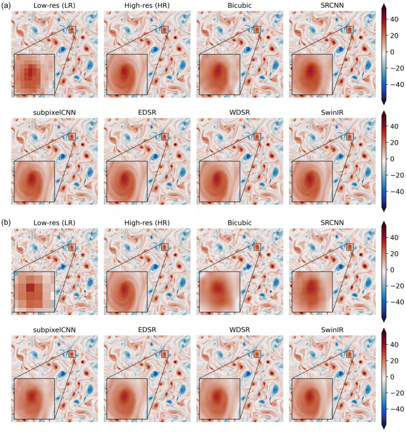
Figure 5: Showcasing baseline SR methods on turbulent fluid flow data ($Re=16000$) under bicubic down-sampling. Here (a) and (b) represent the results of $\times 8$ and $\times 16$ up-sampling tasks.

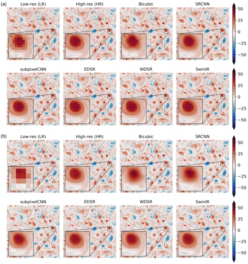
Figure 6: Showcasing baseline SR methods on very turbulent fluid flow data ($Re=32000$) under bicubic down-sampling. Here (a) and (b) represent the results of $\times 8$ and $\times 16$ up-sampling tasks.

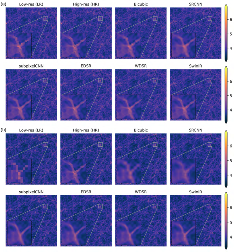
Figure 7: Showcasing baseline SR methods on cosmology data under bicubic down-sampling. Here (a) and (b) represent the results of $\times 8$ and $\times 16$ up-sampling tasks.

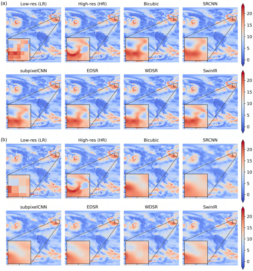
Figure 8: Showcasing baseline SR methods on weather data under bicubic down-sampling. Here (a) and (b) represent the results of $\times 8$ and $\times 16$ up-sampling tasks.

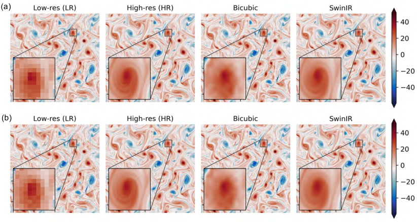
Figure 9: Showcasing baseline SR methods on fluid flow data ($Re=16000$) under uniform down-sampling and noise. Here (a) and (b) show the results of $\times 8$ up-sampling considering $5\%$ and $10\%$ noise, respectively.

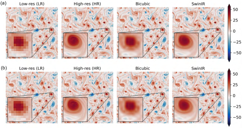
Figure 10: Showcasing baseline SR methods on fluid flow data ($Re=32000$) under uniform down-sampling and noise. Here (a) and (b) show the results of $\times 8$ up-sampling considering $5\%$ and $10\%$ noise, respectively.

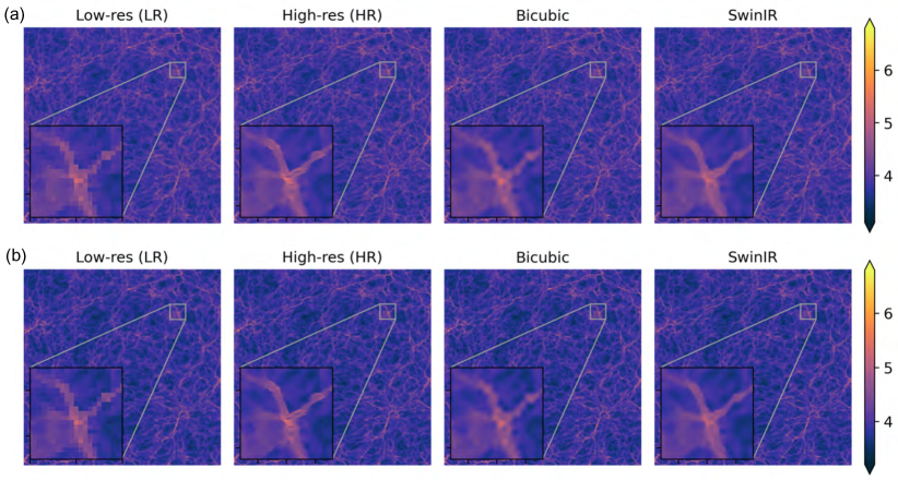
Figure 11: Showcasing baseline SR methods on cosmology data under uniform down-sampling and noise. Here (a) and (b) show the results of $\times 8$ up-sampling considering $5\%$ and $10\%$ noise, respectively.

Figure 12: Showcasing baseline SR methods on weather data under uniform down-sampling and noise. Here (a) and (b) show the results of $\times 8$ up-sampling considering $5\%$ and $10\%$ noise, respectively.

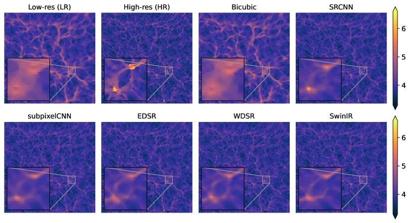
Figure 13: Showcasing baseline SR methods on cosmology data with LR simulation data as inputs. The results are based on $\times 8$ up-sampling.

D.2 Detailed Baseline Performance

The baseline results of all experiments are summarized in the following tables. The error metrics include RFNE ($\downarrow$%), infinity norm (IN$\downarrow$), PSNR ($\uparrow$dB), and SSIM ($\downarrow$). In addition, we also evaluate the performance of physics preservation on fluid flow datasets by measuring continuity loss, as shown in Table 9. The baseline models demonstrate superior SR performance in terms of interpolation errors, indicating the relative ease of the interpolation task compared to extrapolation.

Tables 2-5 reveal that SwinIR outperforms other baseline models in terms of RFNE and SSIM metrics, except for the $\times 8$ up-sampling task on fluid flow data ($Re=16000$) and $\times 16$ up-sampling on cosmology data. In terms of PSNR, EDSR exhibits better performance on fluid flow datasets, while SwinIR demonstrates superiority on cosmology ($\times 8$) and weather data. These results empirically validate the effectiveness of SwinIR in learning multi-scale features. However, as shown in Table 9, the SOTA method SwinIR performs slightly worse than EDSR in preserving physical properties. This implies that achieving satisfactory pixel-level accuracy does not guarantee the preservation of underlying physical properties.

Furthermore, Tables 7-8 present the $\times 8$ SR results of SwinIR on the SuperBench dataset under noisy scenarios with uniform down-sampling degradation. These scenarios simulate real-world experimental conditions, where the existence of noise introduces difficulties in reconstructing high-fidelity scientific data. As the noise level increases, the SR task becomes progressively demanding.

We show the baseline performance of $\times 8$ SR on the LR simulation scenario in Table 6. This task is much more complicated compared to the scenarios involving down-sampling methods for degradation. LR simulation data, in comparison to common down-sampling methods, exhibits a more significant loss of fine-scale and high-frequency features. Moreover, the numerical errors in LR simulations play a crucial role in challenging deep learning models when recovering HR counterparts.

Table 2: Results for fluid flow data ($Re=16000$) with bicubic down-sampling.

	UF	Interpolation Errors				Extrapolation Errors
Baselines	($\times$)	RFNE	IN	PSNR	SSIM	RFNE	IN	PSNR	SSIM	# par.
Bicubic	8	8.66	0.88	36.10	0.96	13.96	1.43	31.41	0.88	0.00 M
SRCNN	8	11.11	1.27	32.13	0.94	15.88	1.62	28.52	0.86	0.07 M
subpixelCNN	8	3.41	0.43	42.08	0.99	4.88	0.61	38.07	0.98	0.34 M
EDSR	8	0.57	0.31	61.30	1.00	1.32	0.47	54.94	1.00	1.67 M
WDSR	8	0.72	0.29	61.32	1.00	1.64	0.52	53.78	1.00	1.40 M
SwinIR	8	0.80	0.35	54.69	1.00	1.46	0.51	49.93	1.00	12.05 M
Bicubic	16	16.56	1.38	30.01	0.89	24.96	2.01	25.64	0.78	0.00 M
SRCNN	16	19.08	1.91	27.54	0.88	27.55	2.35	23.47	0.76	0.07 M
subpixelCNN	16	9.40	0.82	33.06	0.95	12.96	1.07	29.62	0.89	0.67 M
EDSR	16	2.22	0.49	52.64	0.99	5.00	0.77	44.30	0.97	1.81 M
WDSR	16	2.78	0.55	50.52	0.99	5.79	0.84	42.65	0.96	1.62 M
SwinIR	16	2.09	0.55	50.79	1.00	4.52	0.77	44.04	0.97	12.20 M

Table 3: Results for fluid flow data ($Re=32000$) with bicubic down-sampling.

	UF	Interpolation Errors				Extrapolation Errors
Baselines	($\times$)	RFNE	IN	PSNR	SSIM	RFNE	IN	PSNR	SSIM	# par.
Bicubic	8	10.21	0.94	35.30	0.94	17.12	1.64	30.59	0.85	0.00 M
SRCNN	8	11.92	1.13	31.86	0.93	18.73	1.81	27.61	0.83	0.07 M
subpixelCNN	8	5.37	0.48	38.11	0.98	7.86	0.82	34.41	0.95	0.34 M
EDSR	8	1.11	0.35	57.82	1.00	2.83	0.61	50.61	0.99	1.67 M
WDSR	8	1.27	0.29	58.46	1.00	3.26	0.65	49.55	0.99	1.40 M
SwinIR	8	1.09	0.35	55.00	1.00	2.55	0.62	49.47	0.99	12.05 M
Bicubic	16	18.24	1.43	29.49	0.86	28.10	2.21	25.20	0.75	0.00 M
SRCNN	16	21.41	1.73	26.55	0.85	30.32	2.44	23.05	0.73	0.07 M
subpixelCNN	16	10.41	0.87	32.25	0.95	15.80	1.30	28.71	0.86	0.67 M
EDSR	16	3.68	0.53	48.82	0.99	8.34	0.98	40.28	0.93	1.81 M
WDSR	16	4.28	0.54	47.10	0.98	9.15	1.05	39.15	0.92	1.62 M
SwinIR	16	3.80	0.55	44.91	0.99	8.09	0.99	39.11	0.94	12.20 M

Table 4: Results for Cosmology dataset with bicubic down-sampling.

	UF	Interpolation Errors				Extrapolation Errors
Baselines	($\times$)	RFNE	IN	PSNR	SSIM	RFNE	IN	PSNR	SSIM	# par.
Bicubic	8	39.07	10.28	29.78	0.78	40.27	9.06	29.15	0.77	0.00 M
SRCNN	8	36.91	9.40	30.27	0.79	37.84	8.45	29.69	0.77	0.07 M
subpixelCNN	8	20.05	7.76	35.62	0.93	20.08	7.06	35.24	0.93	0.34 M
EDSR	8	19.48	8.33	35.90	0.94	19.52	7.53	35.49	0.94	1.67 M
WDSR	8	21.44	8.67	35.06	0.93	21.41	7.83	34.69	0.93	1.40 M
SwinIR	8	19.38	8.39	35.95	0.94	19.32	7.51	35.59	0.94	12.05 M
Bicubic	16	66.35	11.32	25.18	0.54	67.72	10.11	24.64	0.53	0.00 M
SRCNN	16	61.33	10.48	25.86	0.55	62.58	9.64	25.32	0.54	0.07 M
subpixelCNN	16	47.10	9.58	28.16	0.68	47.71	8.76	27.68	0.67	0.67 M
EDSR	16	46.63	9.98	28.24	0.69	47.23	9.13	27.77	0.68	1.81 M
WDSR	16	48.76	10.24	27.86	0.68	49.36	9.26	27.38	0.67	1.62 M
SwinIR	16	46.62	10.06	28.24	0.69	47.25	9.08	27.76	0.68	12.20 M

Table 5: Results for weather data with bicubic down-sampling.

	UF	Interpolation Errors				Extrapolation Errors
Baselines	($\times$)	RFNE	IN	PSNR	SSIM	RFNE	IN	PSNR	SSIM	# par.
Bicubic	8	17.74	2.67	26.48	0.83	17.67	2.71	26.52	0.83	0.00 M
SRCNN	8	16.47	2.54	27.25	0.84	16.38	2.58	27.30	0.84	0.07 M
subpixelCNN	8	12.07	2.10	30.27	0.89	11.98	2.13	30.33	0.89	0.34 M
EDSR	8	11.90	2.30	30.28	0.89	11.81	2.34	30.35	0.89	1.67 M
WDSR	8	13.20	2.55	29.26	0.88	13.12	2.59	29.32	0.88	1.40 M
SwinIR	8	10.88	2.06	31.22	0.90	10.79	2.10	31.28	0.90	12.05 M
Bicubic	16	27.65	2.94	22.34	0.74	27.55	2.97	22.37	0.74	0.00 M
SRCNN	16	25.31	2.62	23.20	0.75	25.17	2.63	23.26	0.75	0.07 M
subpixelCNN	16	19.55	2.33	25.86	0.81	19.43	2.36	25.92	0.81	0.67 M
EDSR	16	19.24	2.49	25.95	0.81	19.13	2.51	26.01	0.81	1.81 M
WDSR	16	21.19	2.71	24.99	0.79	21.06	2.73	25.05	0.80	1.62 M
SwinIR	16	18.22	2.34	26.39	0.82	18.13	2.37	26.43	0.82	12.20 M

Table 6: Results for cosmology with LR simulation data as inputs.

	UF	Interpolation Errors				Extrapolation Errors
Baselines	($\times$)	RFNE	IN	PSNR	SSIM	RFNE	IN	PSNR	SSIM	# par.
Bicubic	8	91.29	7.04	21.84	0.38	100.68	8.24	21.33	0.33	0.00 M
SRCNN	8	62.33	7.54	25.09	0.51	64.59	8.67	25.10	0.48	0.07 M
subpixelCNN	8	59.41	7.27	25.51	0.53	61.62	8.43	25.51	0.51	0.34 M
EDSR	8	58.26	7.52	25.68	0.54	60.56	8.84	25.66	0.52	1.67 M
WDSR	8	58.61	7.66	25.63	0.54	60.88	8.95	25.61	0.51	1.40 M
SwinIR	8	58.76	7.84	25.61	0.54	60.96	9.08	25.60	0.51	12.05 M

Table 7: Results of SwinIR for SuperBench datasets with uniform down-sampling and $5\%$ noise.

	UF	Interpolation Errors				Extrapolation Errors
Datasets	($\times$)	RFNE	IN	PSNR	SSIM	RFNE	IN	PSNR	SSIM	# par.
Fluid flow (16k)	8	2.58	0.47	47.77	0.99	3.64	0.63	44.23	0.98	12.05 M
Fluid flow (32k)	8	3.60	0.47	45.13	0.98	6.07	0.81	40.75	0.96	12.05 M
Cosmology	8	20.16	8.30	35.58	0.93	20.28	7.55	35.15	0.93	12.05 M
Weather	8	11.96	2.15	30.01	0.89	11.89	2.21	30.04	0.89	12.05 M

Table 8: Results of SwinIR for SuperBench datasets with uniform down-sampling and $10\%$ noise.

	UF	Interpolation Errors				Extrapolation Errors
Datasets	($\times$)	RFNE	IN	PSNR	SSIM	RFNE	IN	PSNR	SSIM	# par.
Fluid flow (16k)	8	3.98	0.50	43.52	0.98	5.03	0.69	40.66	0.97	12.05 M
Fluid flow (32k)	8	4.90	0.50	42.52	0.97	7.35	0.93	38.92	0.95	12.05 M
Cosmology	8	21.10	8.32	35.17	0.92	21.25	7.57	34.73	0.91	12.05 M
Weather	8	12.92	2.15	29.11	0.87	12.84	2.22	29.15	0.88	12.05 M

Table 9: Results of physics errors on fluid flow data.

	UF	Down-sampling	Noise	$Re=16000$		$Re=32000$
Baselines	($\times$)	methods	(%)	Interp.	Extrap.	Interp.	Extrap.	# par.
Bicubic	8	Bicubic	0	0.38	1.13	0.49	1.54	0.00 M
SRCNN	8	Bicubic	0	11.06	32.96	15.96	62.68	0.07 M
subpixelCNN	8	Bicubic	0	10.59	22.63	15.09	35.53	0.34 M
EDSR	8	Bicubic	0	0.01	0.04	0.01	0.05	1.67 M
WDSR	8	Bicubic	0	0.07	0.35	0.07	0.40	1.40 M
SwinIR	8	Bicubic	0	0.03	0.18	0.03	0.18	12.05 M
Bicubic	16	Bicubic	0	0.43	1.50	0.55	1.88	0.00 M
SRCNN	16	Bicubic	0	31.60	60.63	21.68	58.74	0.07 M
subpixelCNN	16	Bicubic	0	21.19	41.50	22.53	46.50	0.67 M
EDSR	16	Bicubic	0	0.01	0.06	0.02	0.10	1.81 M
WDSR	16	Bicubic	0	0.14	0.43	0.23	0.68	1.62 M
SwinIR	16	Bicubic	0	0.05	0.20	0.06	0.25	12.20 M
SwinIR	8	Uniform	5	0.04	0.15	0.04	0.17	12.05 M
SwinIR	8	Uniform	10	0.05	0.17	0.06	0.23	12.05 M

D.3 Comprehensive Analysis

Based on the results presented in the Detailed Baseline Performance (Section D.2), we complement the analysis by visualizing the baseline performances on SuperBench dataset. Specifically, we show the relationships between error metrics and model parameters in Figure 14.

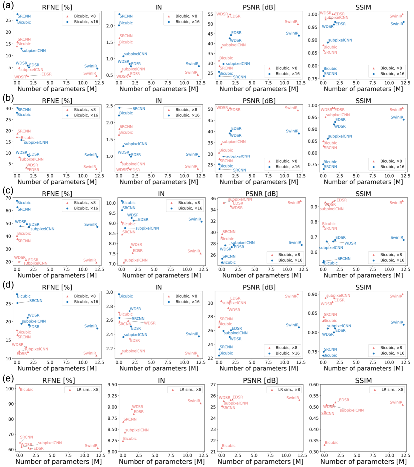
Figure 14: Visualization of errors versus model parameters on SuperBench dataset. (a)-(d) show the baseline performances of fluid flow ($Re=16000$ and $Re=32000$), cosmology and weather datasets, respectively. They are based on bicubic down-sampling degradation. (e) presents the result on the cosmology dataset with LR simulation data as inputs.

Appendix E Reproducibility

The code for processing the datasets, running baseline models, and evaluating model performance is publicly available in our GitHub repository. The README file contains system requirements, installation instructions, and running examples. Detailed training information is provided in Appendix C.

Appendix F Data Hosting, Licensing, Format, and Maintenance

SuperBench is a collaborative effort involving a diverse team from different institutes, including Lawrence Berkeley National Lab (LBNL), University of California at Berkeley, International Computer Science Institute (ICSI), and Oklahoma State University. In this section, we provide detailed information on SuperBench dataset, such as data hosting, data licensing, data format, and maintenance plans.

F.1 Data Hosting

SuperBench is hosted on the shared file systems of the National Energy Research Scientific Computing Center (NERSC) platform. The data is publicly available with the following link (https://portal.nersc.gov/project/dasrepo/superbench/superbench_v1.tar). Users can download the dataset locally by either clicking on the provided link or using the wget command in the terminal. In addition, the code used to process the dataset and run the baseline models is available on our GitHub repository (https://github.com/erichson/SuperBench).

F.2 Data Licensing

SuperBench is released under an Open Data Commons Attribution License. The fluid flow and cosmology datasets are produced by the authors themselves. The ERA5 dataset provided in SuperBench is available in the public domain. It is free to use for research purposes.

F.3 Data Format

SuperBench consists of five distinct data files: NSKT ($Re=16000$); NSKT ($Re=32000$); cosmology data; cosmology data with LR simulation; and weather data (ERA5). Each data file includes five sub-directories: one training dataset (train file), two validation datasets (valid_1 and valid_2) files for validating interpolation and extrapolation performance), and two testing datasets (test_1 and test_2) files for testing interpolation and extrapolation performance). More details about the design of interpolation and extrapolation datasets can be found in Appendix A. The data in each sub-directory is stored in the HDF5 [19] binary data format. The code for loading/reading each dataset is provided in the SuperBench repository.

F.4 Maintenance Plan

SuperBench will be maintained by LBNL. Any encountered issues will be promptly addressed and updated in the provided data and GitHub repository links. Moreover, as highlighted in the Conclusion (Section 6), SuperBench offers an extendable framework to include new datasets and baseline models. We encourage contributions from the SciML community and envision SuperBench as a collaborative platform. Future versions of SuperBench dataset will be released.

References

- [1] Amir Aghamousa et al. The DESI Experiment Part I: Science,Targeting, and Survey Design. 10 2016.
- [2] Eirikur Agustsson and Radu Timofte. NTIRE 2017 Challenge on Single Image Super-Resolution: Dataset and Study. In 2017 IEEE Conference on Computer Vision and Pattern Recognition Workshops, CVPR Workshops 2017, Honolulu, HI, USA, July 21-26, 2017, pages 1122–1131. IEEE Computer Society, 2017.
- [3] A. S. Almgren, J. B. Bell, M. J. Lijewski, Z. Lukić, and E. Van Andel. Nyx: A Massively Parallel AMR Code for Computational Cosmology. The Astrophysical Journal, 765:39, March 2013.
- [4] Marcelo A. Alvarez, Arka Banerjee, Simon Birrer, Salman Habib, Katrin Heitmann, Zarija Lukić, Julian B. Muñoz, Yuuki Omori, Hyunbae Park, Annika H. G. Peter, Jean Sexton, and Yi-Ming Zhong. Snowmass2021 Computational Frontier White Paper: Cosmological Simulations and Modeling. arXiv e-prints, page arXiv:2203.07347, March 2022.
- [5] Saeed Anwar, Salman Khan, and Nick Barnes. A Deep Journey into Super-Resolution: A Survey. ACM Computing Surveys (CSUR), 53(3):1–34, 2020.
- [6] Akio Arakawa. Computational Design for Long-term Numerical Integration of the Equations of Fluid Motion: Two-dimensional Incompressible Flow. Part I. Journal of Computational Physics, 135(2):103–114, 1997.
- [7] Md Rifat Arefin, Vincent Michalski, Pierre-Luc St-Charles, Alfredo Kalaitzis, Sookyung Kim, Samira E Kahou, and Yoshua Bengio. Multi-image Super-resolution for Remote Sensing Using Deep Recurrent Networks. In Proceedings of the IEEE/CVF Conference on Computer Vision and Pattern Recognition Workshops, pages 206–207, 2020.
- [8] Tianshu Bao, Shengyu Chen, Taylor T Johnson, Peyman Givi, Shervin Sammak, and Xiaowei Jia. Physics Guided Neural Networks for Spatio-temporal Super-resolution of Turbulent Flows. In Uncertainty in Artificial Intelligence, pages 118–128. PMLR, 2022.
- [9] Marco Bevilacqua, Aline Roumy, Christine Guillemot, and Marie-Line Alberi-Morel. Low-Complexity Single-Image Super-Resolution based on Nonnegative Neighbor Embedding. In Richard Bowden, John P. Collomosse, and Krystian Mikolajczyk, editors, British Machine Vision Conference, BMVC 2012, Surrey, UK, September 3-7, 2012, pages 1–10. BMVA Press, 2012.
- [10] Mathis Bode, Michael Gauding, Zeyu Lian, Dominik Denker, Marco Davidovic, Konstantin Kleinheinz, Jenia Jitsev, and Heinz Pitsch. Using Physics-informed Enhanced Super-resolution Generative Adversarial Networks for Subfilter Modeling in Turbulent Reactive Flows. Proceedings of the Combustion Institute, 38(2):2617–2625, 2021.
- [11] Jianrui Cai, Hui Zeng, Hongwei Yong, Zisheng Cao, and Lei Zhang. Toward Real-world Single Image Super-resolution: A New Benchmark and A New Model. In Proceedings of the IEEE/CVF International Conference on Computer Vision, pages 3086–3095, 2019.
- [12] Kelvin CK Chan, Xintao Wang, Xiangyu Xu, Jinwei Gu, and Chen Change Loy. GLEAN: Generative Latent Bank for Large-factor Image Super-resolution. In Proceedings of the IEEE/CVF Conference on Computer Vision and Pattern Recognition, pages 14245–14254, 2021.
- [13] Hanting Chen, Yunhe Wang, Tianyu Guo, Chang Xu, Yiping Deng, Zhenhua Liu, Siwei Ma, Chunjing Xu, Chao Xu, and Wen Gao. Pre-trained Image Processing Transformer. In Proceedings of the IEEE/CVF Conference on Computer Vision and Pattern Recognition, pages 12299–12310, 2021.
- [14] Chao Dong, Chen Change Loy, Kaiming He, and Xiaoou Tang. Image Super-resolution Using Deep Convolutional Networks. IEEE Transactions on Pattern Analysis and Machine Intelligence, 38(2):295–307, 2015.
- [15] Chao Dong, Chen Change Loy, and Xiaoou Tang. Accelerating the Super-Resolution Convolutional Neural Network. In Bastian Leibe, Jiri Matas, Nicu Sebe, and Max Welling, editors, Computer Vision - ECCV 2016 - 14th European Conference, Amsterdam, The Netherlands, October 11-14, 2016, Proceedings, Part II, volume 9906 of Lecture Notes in Computer Science, pages 391–407. Springer, 2016.
- [16] C. Edwards. Neural Networks Learn to Speed Up Simulations. Communications of the ACM, 65(5):27–29, 2022.
- [17] N Benjamin Erichson, Lionel Mathelin, Zhewei Yao, Steven L Brunton, Michael W Mahoney, and J Nathan Kutz. Shallow Neural Networks for Fluid Flow Reconstruction with Limited Sensors. Proceedings of the Royal Society A, 476(2238):20200097, 2020.
- [18] Soheil Esmaeilzadeh, Kamyar Azizzadenesheli, Karthik Kashinath, Mustafa Mustafa, Hamdi A Tchelepi, Philip Marcus, Mr Prabhat, Anima Anandkumar, et al. Meshfreeflownet: A Physics-constrained Deep Continuous Space-time Super-resolution Framework. In SC20: International Conference for High Performance Computing, Networking, Storage and Analysis, pages 1–15. IEEE, 2020.
- [19] Mike Folk, Gerd Heber, Quincey Koziol, Elena Pourmal, and Dana Robinson. An Overview of the HDF5 Technology Suite and its Applications. In Proceedings of the EDBT/ICDT 2011 Workshop on Array Databases, pages 36–47, 2011.
- [20] Kai Fukami, Koji Fukagata, and Kunihiko Taira. Super-resolution Reconstruction of Turbulent Flows with Machine Learning. Journal of Fluid Mechanics, 870:106–120, 2019.
- [21] Kai Fukami, Koji Fukagata, and Kunihiko Taira. Machine-learning-based Spatio-temporal Super Resolution Reconstruction of Turbulent Flows. Journal of Fluid Mechanics, 909, 2021.
- [22] Kai Fukami, Koji Fukagata, and Kunihiko Taira. Super-Resolution Analysis via Machine Learning: A Survey for Fluid Flows. arXiv preprint arXiv:2301.10937, 2023.
- [23] Kai Fukami, Romit Maulik, Nesar Ramachandra, Koji Fukagata, and Kunihiko Taira. Global Field Reconstruction from Sparse Sensors with Voronoi Tessellation-assisted Deep Learning. Nature Machine Intelligence, 3(11):945–951, 2021.
- [24] Han Gao, Luning Sun, and Jian-Xun Wang. Super-resolution and Denoising of Fluid Flow Using Physics-informed Convolutional Neural Networks without High-resolution Labels. Physics of Fluids, 33(7):073603, 2021.
- [25] Hayit Greenspan. Super-resolution in Medical Imaging. The Computer Journal, 52(1):43–63, 2009.
- [26] Hans Hersbach, Bill Bell, Paul Berrisford, Shoji Hirahara, András Horányi, Joaquín Muñoz-Sabater, Julien Nicolas, Carole Peubey, Raluca Radu, Dinand Schepers, et al. The ERA5 Global Reanalysis. Quarterly Journal of the Royal Meteorological Society, 146(730):1999–2049, 2020.
- [27] Jia-Bin Huang, Abhishek Singh, and Narendra Ahuja. Single Image Super-resolution from Transformed Self-exemplars. In Proceedings of the IEEE Conference on Computer Vision and Pattern Recognition, pages 5197–5206, 2015.
- [28] Jithin Saji Isaac and Ramesh Kulkarni. Super Resolution Techniques for Medical Image Processing. In 2015 International Conference on Technologies for Sustainable Development (ICTSD), pages 1–6. IEEE, 2015.
- [29] Eugenia Kalnay. Atmospheric Modeling, Data Assimilation and Predictability. Cambridge university press, 2003.
- [30] George Em Karniadakis, Ioannis G Kevrekidis, Lu Lu, Paris Perdikaris, Sifan Wang, and Liu Yang. Physics-informed Machine Learning. Nature Reviews Physics, 3(6):422–440, 2021.
- [31] Jiwon Kim, Jung Kwon Lee, and Kyoung Mu Lee. Accurate Image Super-resolution Using Very Deep Convolutional Networks. In Proceedings of the IEEE Conference on Computer Vision and Pattern Recognition, pages 1646–1654, 2016.
- [32] Diederik P. Kingma and Jimmy Ba. Adam: A Method for Stochastic Optimization. In Yoshua Bengio and Yann LeCun, editors, 3rd International Conference on Learning Representations, ICLR 2015, San Diego, CA, USA, May 7-9, 2015, Conference Track Proceedings, 2015.
- [33] A. S. Krishnapriyan, A. F. Queiruga, N. B. Erichson, and M. W. Mahoney. Learning Continuous Models for Continuous Physics. Technical Report Preprint: arXiv:2202.08494, 2022.
- [34] Aditi Krishnapriyan, Amir Gholami, Shandian Zhe, Robert Kirby, and Michael W Mahoney. Characterizing Possible Failure Modes in Physics-informed Neural Networks. Advances in Neural Information Processing Systems, 34:26548–26560, 2021.
- [35] Christian Ledig, Lucas Theis, Ferenc Huszár, Jose Caballero, Andrew Cunningham, Alejandro Acosta, Andrew Aitken, Alykhan Tejani, Johannes Totz, Zehan Wang, et al. Photo-realistic Single Image Super-resolution Using A Generative Adversarial Network. In Proceedings of the IEEE Conference on Computer Vision and Pattern Recognition, pages 4681–4690, 2017.
- [36] Zhan Li, Qingyu Peng, Bir Bhanu, Qingfeng Zhang, and Haifeng He. Super Resolution for Astronomical Observations. Astrophysics and Space Science, 363(5):1–15, 2018.
- [37] Jingyun Liang, Jiezhang Cao, Guolei Sun, Kai Zhang, Luc Van Gool, and Radu Timofte. Swinir: Image Restoration Using Swin Transformer. In Proceedings of the IEEE/CVF International Conference on Computer Vision, pages 1833–1844, 2021.
- [38] Bee Lim, Sanghyun Son, Heewon Kim, Seungjun Nah, and Kyoung Mu Lee. Enhanced Deep Residual Networks for Single Image Super-resolution. In Proceedings of the IEEE Conference on Computer Vision and Pattern Recognition Workshops, pages 136–144, 2017.
- [39] Bo Liu, Jiupeng Tang, Haibo Huang, and Xi-Yun Lu. Deep Learning Methods for Super-resolution Reconstruction of Turbulent Flows. Physics of Fluids, 32(2):025105, 2020.
- [40] Ze Liu, Yutong Lin, Yue Cao, Han Hu, Yixuan Wei, Zheng Zhang, Stephen Lin, and Baining Guo. Swin Transformer: Hierarchical Vision Transformer using Shifted Windows. In 2021 IEEE/CVF International Conference on Computer Vision, ICCV 2021, Montreal, QC, Canada, October 10-17, 2021, pages 9992–10002. IEEE, 2021.
- [41] Ilya Loshchilov and Frank Hutter. Decoupled Weight Decay Regularization. In 7th International Conference on Learning Representations, ICLR 2019, New Orleans, LA, USA, May 6-9, 2019. OpenReview.net, 2019.
- [42] LSST Science Collaboration. LSST Science Book, Version 2.0. arXiv e-prints, page arXiv:0912.0201, December 2009.
- [43] Lu Lu, Pengzhan Jin, Guofei Pang, Zhongqiang Zhang, and George Em Karniadakis. Learning Nonlinear Operators via DeepONet based on the Universal Approximation Theorem of Operators. Nature Machine Intelligence, 3(3):218–229, 2021.
- [44] Lu Lu, Xuhui Meng, Zhiping Mao, and George Em Karniadakis. DeepXDE: A Deep Learning Library for Solving Differential Equations. SIAM Review, 63(1):208–228, 2021.
- [45] Andreas Lugmayr, Martin Danelljan, and Radu Timofte. Unsupervised Learning for Real-world Super-resolution. In 2019 IEEE/CVF International Conference on Computer Vision Workshop (ICCVW), pages 3408–3416. IEEE, 2019.
- [46] Zarija Lukić, Casey W Stark, Peter Nugent, Martin White, Avery A Meiksin, and Ann Almgren. The Lyman Forest in Optically Thin Hydrodynamical Simulations. Monthly Notices of the Royal Astronomical Society, 446(4):3697–3724, 2015.
- [47] Nina A Maksimova, Lehman H Garrison, Daniel J Eisenstein, Boryana Hadzhiyska, Sownak Bose, and Thomas P Satterthwaite. AbacusSummit: A Massive Set of High-accuracy, High-resolution N-body Simulations. Monthly Notices of the Royal Astronomical Society, 508(3):4017–4037, 09 2021.
- [48] David Martin, Charless Fowlkes, Doron Tal, and Jitendra Malik. A Database of Human Segmented Natural Images and its application to Evaluating Segmentation Algorithms and Measuring Ecological Statistics. In Proceedings Eighth IEEE International Conference on Computer Vision. ICCV 2001, volume 2, pages 416–423. IEEE, 2001.
- [49] Brian B Moser, Federico Raue, Stanislav Frolov, Sebastian Palacio, Jörn Hees, and Andreas Dengel. Hitchhiker’s Guide to Super-Resolution: Introduction and Recent Advances. IEEE Transactions on Pattern Analysis and Machine Intelligence, 2023.
- [50] Kamal Nasrollahi and Thomas B Moeslund. Super-resolution: A Comprehensive Survey. Machine Vision and Applications, 25(6):1423–1468, 2014.
- [51] Geoffrey Négiar, Michael W Mahoney, and Aditi S Krishnapriyan. Learning Differentiable Solvers for Systems with Hard Constraints. arXiv preprint arXiv:2207.08675, 2022.
- [52] Sung Cheol Park, Min Kyu Park, and Moon Gi Kang. Super-resolution Image Reconstruction: A Technical Overview. IEEE Signal Processing Magazine, 20(3):21–36, 2003.
- [53] Suraj Pawar, Omer San, Adil Rasheed, and Prakash Vedula. Frame Invariant Neural Network Closures for Kraichnan Turbulence. Physica A: Statistical Mechanics and its Applications, 609:128327, 2023.
- [54] Klaus G Puschmann and Franz Kneer. On Super-resolution in Astronomical Imaging. Astronomy & Astrophysics, 436(1):373–378, 2005.
- [55] Maziar Raissi, Paris Perdikaris, and George E Karniadakis. Physics-informed Neural Networks: A Deep Learning Framework for Solving Forward and Inverse Problems Involving Nonlinear Partial Differential Equations. Journal of Computational Physics, 378:686–707, 2019.
- [56] Stephan Rasp, Peter D Dueben, Sebastian Scher, Jonathan A Weyn, Soukayna Mouatadid, and Nils Thuerey. WeatherBench: A Benchmark Data Set for Data-driven Weather Forecasting. Journal of Advances in Modeling Earth Systems, 12(11):e2020MS002203, 2020.
- [57] Pu Ren, Chengping Rao, Yang Liu, Zihan Ma, Qi Wang, Jian-Xun Wang, and Hao Sun. Physics-informed Deep Super-resolution for Spatiotemporal Data. arXiv preprint arXiv:2208.01462, 2022.
- [58] Robin Rombach, Andreas Blattmann, Dominik Lorenz, Patrick Esser, and Björn Ommer. High-resolution Image Synthesis with Latent Diffusion Models. In Proceedings of the IEEE/CVF Conference on Computer Vision and Pattern Recognition, pages 10684–10695, 2022.
- [59] Chitwan Saharia, Jonathan Ho, William Chan, Tim Salimans, David J Fleet, and Mohammad Norouzi. Image Super-resolution via Iterative Refinement. IEEE Transactions on Pattern Analysis and Machine Intelligence, 2022.
- [60] Joao Satiro, Kamal Nasrollahi, Paulo L Correia, and Thomas B Moeslund. Super-resolution of Facial Images in Forensics Scenarios. In 2015 International Conference on Image Processing Theory, Tools and Applications (IPTA), pages 55–60. IEEE, 2015.
- [61] Tapio Schneider, João Teixeira, Christopher S. Bretherton, Florent Brient, Kyle G. Pressel, Christoph Schär, and A. Pier Siebesma. Climate Goals and Computing the Future of Clouds. Nature Climate Change, 7:3–5, 2017.
- [62] Wenzhe Shi, Jose Caballero, Ferenc Huszar, Johannes Totz, Andrew P. Aitken, Rob Bishop, Daniel Rueckert, and Zehan Wang. Real-Time Single Image and Video Super-Resolution Using an Efficient Sub-Pixel Convolutional Neural Network. In Proceedings of the IEEE Conference on Computer Vision and Pattern Recognition (CVPR), June 2016.
- [63] Akshay Subramaniam, Man Long Wong, Raunak D Borker, Sravya Nimmagadda, and Sanjiva K Lele. Turbulence Enrichment Using Physics-informed Generative Adversarial Networks. arXiv preprint arXiv:2003.01907, 2020.
- [64] Ying Tai, Jian Yang, and Xiaoming Liu. Image Super-resolution via Deep Recursive Residual Network. In Proceedings of the IEEE Conference on Computer Vision and Pattern Recognition, pages 3147–3155, 2017.
- [65] Makoto Takamoto, Timothy Praditia, Raphael Leiteritz, Daniel MacKinlay, Francesco Alesiani, Dirk Pflüger, and Mathias Niepert. PDEBench: An Extensive Benchmark for Scientific Machine Learning. Advances in Neural Information Processing Systems, 35:1596–1611, 2022.
- [66] Jeyan Thiyagalingam, Mallikarjun Shankar, Geoffrey Fox, and Tony Hey. Scientific Machine Learning Benchmarks. Nature Reviews Physics, 4(6):413–420, 2022.
- [67] Jing Tian and Kai-Kuang Ma. A Survey on Super-resolution Imaging. Signal, Image and Video Processing, 5(3):329–342, 2011.
- [68] Radu Timofte, Shuhang Gu, Jiqing Wu, and Luc Van Gool. NTIRE 2018 Challenge on Single Image Super-Resolution: Methods and Results. In 2018 IEEE Conference on Computer Vision and Pattern Recognition Workshops, CVPR Workshops 2018, Salt Lake City, UT, USA, June 18-22, 2018, pages 852–863. Computer Vision Foundation / IEEE Computer Society, 2018.
- [69] Tong Tong, Gen Li, Xiejie Liu, and Qinquan Gao. Image Super-resolution Using Dense Skip Connections. In Proceedings of the IEEE International Conference on Computer Vision, pages 4799–4807, 2017.
- [70] JD Van Ouwerkerk. Image Super-resolution Survey. Image and Vision Computing, 24(10):1039–1052, 2006.
- [71] Ricardo Vinuesa and Steven L Brunton. Enhancing Computational Fluid Dynamics with Machine Learning. Nature Computational Science, 2(6):358–366, 2022.
- [72] Chulin Wang, Eloisa Bentivegna, Wang Zhou, Levente Klein, and Bruce Elmegreen. Physics-informed Neural Network Super Resolution for Advection-diffusion Models. arXiv preprint arXiv:2011.02519, 2020.
- [73] Rui Wang, Karthik Kashinath, Mustafa Mustafa, Adrian Albert, and Rose Yu. Towards Physics-informed Deep Learning for Turbulent Flow Prediction. In Proceedings of the 26th ACM SIGKDD International Conference on Knowledge Discovery & Data Mining, pages 1457–1466, 2020.
- [74] Xintao Wang, Ke Yu, Shixiang Wu, Jinjin Gu, Yihao Liu, Chao Dong, Yu Qiao, and Chen Change Loy. ESRGAN: Enhanced Super-resolution Generative Adversarial Networks. In Proceedings of the European Conference on Computer Vision (ECCV) Workshops, pages 0–0, 2018.
- [75] Zhihao Wang, Jian Chen, and Steven CH Hoi. Deep Learning for Image Super-resolution: A Survey. IEEE Transactions on Pattern Analysis and Machine Intelligence, 43(10):3365–3387, 2020.
- [76] Zhou Wang, Alan C Bovik, Hamid R Sheikh, and Eero P Simoncelli. Image Quality Assessment: from Error Visibility to Structural Similarity. IEEE Transactions on Image Processing, 13(4):600–612, 2004.
- [77] You Xie, Erik Franz, Mengyu Chu, and Nils Thuerey. tempoGAN: A Temporally Coherent, Volumetric GAN for Super-resolution Fluid Flow. ACM Trans. Graph., 37(4):95, 2018.
- [78] Fuzhi Yang, Huan Yang, Jianlong Fu, Hongtao Lu, and Baining Guo. Learning Texture Transformer Network for Image Super-resolution. In Proceedings of the IEEE/CVF Conference on Computer Vision and Pattern Recognition, pages 5791–5800, 2020.
- [79] Jianchao Yang, John Wright, Thomas Huang, and Yi Ma. Image Super-resolution as Sparse Representation of Raw Image Patches. In 2008 IEEE Conference on Computer Vision and Pattern Recognition, pages 1–8. IEEE, 2008.
- [80] Jianchao Yang, John Wright, Thomas S Huang, and Yi Ma. Image Super-resolution via Sparse Representation. IEEE Transactions on Image Processing, 19(11):2861–2873, 2010.
- [81] Christopher Yeh, Chenlin Meng, Sherrie Wang, Anne Driscoll, Erik Rozi, Patrick Liu, Jihyeon Janel Lee, Marshall Burke, David B. Lobell, and Stefano Ermon. SustainBench: Benchmarks for Monitoring the Sustainable Development Goals with Machine Learning. In Joaquin Vanschoren and Sai-Kit Yeung, editors, Proceedings of the Neural Information Processing Systems Track on Datasets and Benchmarks 1, NeurIPS Datasets and Benchmarks 2021, December 2021, virtual, 2021.
- [82] Jiahui Yu, Yuchen Fan, Jianchao Yang, Ning Xu, Zhaowen Wang, Xinchao Wang, and Thomas Huang. Wide Activation for Efficient and Accurate Image Super-resolution. arXiv preprint arXiv:1808.08718, 2018.
- [83] Jian Yu and Jan S Hesthaven. Flowfield Reconstruction Method Using Artificial Neural Network. AIAA Journal, 57(2):482–498, 2019.
- [84] Roman Zeyde, Michael Elad, and Matan Protter. On Single Image Scale-Up Using Sparse-Representations. In Jean-Daniel Boissonnat, Patrick Chenin, Albert Cohen, Christian Gout, Tom Lyche, Marie-Laurence Mazure, and Larry L. Schumaker, editors, Curves and Surfaces - 7th International Conference, Avignon, France, June 24-30, 2010, Revised Selected Papers, volume 6920 of Lecture Notes in Computer Science, pages 711–730. Springer, 2010.
- [85] Wenlong Zhang, Yihao Liu, Chao Dong, and Yu Qiao. RankSRGAN: Generative Adversarial Networks with Ranker for Image Super-resolution. In Proceedings of the IEEE/CVF International Conference on Computer Vision, pages 3096–3105, 2019.
- [86] Yulun Zhang, Yapeng Tian, Yu Kong, Bineng Zhong, and Yun Fu. Residual Dense Network for Image Super-resolution. In Proceedings of the IEEE Conference on Computer Vision and Pattern Recognition, pages 2472–2481, 2018.