On a recent calculation of the mass spectra of quarkonia using the Cornell potential with spin-spin interactions

Abstract

We analyse a recent application of the Cornell potential with spin-spin interaction to the mass spectra of quarkonia and show that the authors have in fact used the Kratzer-Fues potential. They inadvertently converted one potential into the other by means of an invalid transformation.

In a paper published recently, Omugbe et al[1] tried to it experimental data by means of the solutions of the non-relativistic Schrödinger equation with the Cornell potential with spin-spin interaction. They carried out a coordinate transformation and two approximations that enabled them to derive an eigenvalue equation that can be solved by the Nikiforov-Uvarov method. In this way they obtained analytical approximate expressions for the eigenvalues and eigenfunctions. In this short note we analyse the mathematical procedure followed by those authors.

In order to study a meson mass spectra Omugbe et al[1] proposed the Cornell potential with spin-spin interaction

$$V(r) = -\frac{4\alpha_{s}}{3r}+br+C_{s}e^{-\sigma^{2}r^{2}},$$

$$C_{s} = 16\alpha_{s}\pi\left(\frac{\sigma}{\sqrt{\pi}}\right)^{3}\frac{s(s+1)-\frac{3}{2}}{9m_{q}m_{\bar{q}}},$$ (1)

where $\alpha_{s}$, $b$ and $\sigma$ are adjustable model parameters, $s$ is the spin quantum number and $m_{q}$, $m_{\bar{q}}$ are the masses of the quark and antiquark, respectively. They focused on the radial part of the eigenvalue equation written as

$$-\frac{\hbar^{2}}{2\mu}\frac{d^{2}\psi_{nl}(r)}{dr^{2}}+\left[V(r)+\frac{\hbar^{2}l(l+1)}{2\mu r^{2}}\right]\psi_{nl}(r)=E_{nl}\psi_{nl}(r),$$ (2)

where $\mu$ is the reduced mass and $l$ the rotational quantum number. The authors did not mention it explicitly but we assume that the boundary conditions are $\psi_{nl}(0)=0$ and $\psi_{nl}(r\rightarrow\infty)=0$ provided that $b>0$.

Since the eigenvalue equation (2) is not exactly solvable, Omugbe er al[1] resorted to a series of approximations. The first one consists of expanding the Gaussian term to second order which produces the approximate potential

$$V^{OEA}(r)=C_{s}-\frac{4\alpha_{s}}{3r}+br-C_{s}\sigma^{2}r^{2}.$$ (3)

For $s=0$ this potential supports bound states because $C_{0}<0$; however, for $s=1$ there are no bound states because $C_{1}>0$ and the resulting potential is unbounded from below. In other words: this approximation is unsuitable for triplet states. Omugbe et al[1] overlooked this limitation that was overcome by the second incorrect approximation discussed below.

Omugbe et al[1] carried out the variable transformation $q=1/r$ that leads to

$$\frac{d^{2}\psi}{dq^{2}}+\frac{2}{q}\frac{d\psi}{dq}+\frac{1}{q^{4}}\left(\epsilon_{nl}+aq-\frac{c}{q}+\frac{d}{q^{2}}-Lq^{2}\right)\psi=0,$$ (4)

where all the parameters are given in their paper. Note that we have taken into consideration that $2q/q^{2}=2/q$. At this point, Omugbe et al[1] argued as follows: “However, we must put the equation into a standard form using an approximation scheme by expanding $c/q$ and $d/q^{2}$ in power series to second-order around $q_{0}$ ($\delta=1/q_{0}$) which is assumed to be the characteristic radius of mesons.” From this second approximation they obtained the highly inaccurate expressions

$$\frac{c}{q} = c\left(\frac{3}{\delta}-\frac{3q}{\delta^{2}}+\frac{q^{2}}{\delta^{3}}\right),$$

$$\frac{d}{q^{2}} = d\left(\frac{6}{\delta^{2}}-\frac{8q}{\delta^{3}}+\frac{3q^{2}}{\delta^{4}}\right).$$ (5)

Since, for each of these equations, the left-hand side is completely different from the right-hand side, as shown in figures 1 and 2 for $\delta=0.7$, we conclude that Omugbe et al[1] transformed the original model into another one with completely different behaviour at $q\rightarrow 0$ and $q\rightarrow\infty$, given by the eigenvalue equation

$$\frac{d^{2}\psi}{dq^{2}}+\frac{2}{q}\frac{d\psi}{dq}+\frac{1}{q^{4}}\left(-Aq^{2}+Bq-C\right)\psi=0,$$ (6)

where all the parameters are given in their paper. Note that, once more, we have taken into account that $2q/q^{2}=2/q$.

The eigenvalue equation (6) describes a physical model that is completely different from the original one given by $V(r)$ (1) and even from the approximate one based on $V^{OEA}(r)$ (3). In fact, if we substitute $q=1/r$ into equation (6) we obtain the eigenvalue equation

$$\frac{d^{2}\psi}{dr^{2}}+\left(\frac{B}{r}-\frac{A}{r^{2}}-C\right)\psi=0,$$ (7)

where $V^{KF}(r)=\frac{\hbar^{2}}{2\mu}\left(-\frac{B}{r}+\frac{A}{r^{r}}\right)$ resembles the Kratzer-Fues potential[2, 3]. The eigenvalue equation (7) can be easily solved by means of the simple and straightforward Frobenius (power-series) method[4]. Omugbe et al[1] applied the far more complicated Nikiforov-Uvarov method to equation (6) and obtained the eigenvalues

$$E_{nl}^{OEA}=\Gamma_{0}-\frac{\mu}{2\hbar^{2}}\left(\frac{\Gamma_{1}}{n+\Gamma_{2}}\right)^{2},$$ (8)

where the parameters $\Gamma_{j}$ are given in their paper. As expected, this spectrum resembles the one for the Kratzer-Fues potential[3, 4].

It is illustrative to compare the spectrum of the original model based on the potential-energy function (1) and the one used by Omugbe et al[1] in their study of the physical problem given by either equation (7) or (6). Since the original model potential is unbounded from above (increases as $br$ when $r\rightarrow\infty$), we conclude that $E_{nl}\rightarrow\infty$ when $n\rightarrow\infty$. On the other hand, $E_{nl}^{OEA}\rightarrow\Gamma_{0}$ when $n\rightarrow\infty$. The reason for this gross qualitative discrepancy is due to the transformations (5) that convert the original model into a completely different one.

Summarizing: Omugbe et al[1] claimed that they fitted experimental data to the solutions of the Schrödinger equation for the Cornell potential with spin-spin interaction when the true fact is that they used the Kratzer-Fues potential that exhibits a completely different spectrum. The origin of this mistake can be traced back to the two invalid transformations discussed above.

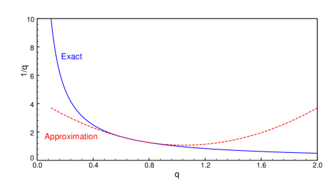
Figure 1: Exact values of $1/q$ (blue, continuous line) and the approximation (5) (red, dashed line) for $\delta=0.7$

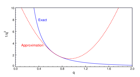
Figure 2: Exact values of $1/q^{2}$ (blue, continuous line) and the approximation (5) (red, dashed line) for $\delta=0.7$

References

- [1] E. Omugbe, E. P. Inyang, I. J. Njoku, C. Martínez-Flores, A. Jahanshir, I. B. Okon, E. S. Eyube, R. Horchani, and C.A. Onate, Nucl. Phys. A 1034 (2023) 122653.
- [2] A. Kratzer, Z. Physik 3 (1920) 289-307.
- [3] E. Fues, Ann. Phys. 386 (1926) 281-313.
- [4] F. M. Fernández, J. Math. Phys. 62 (2021) 064101.