Quasiparticle spectroscopy in technologically-relevant niobium using London penetration depth measurements

Abstract

London penetration depth was measured in niobium foils, thin films, single crystals, and superconducting radio-frequency (SRF) cavity pieces cut out from different places. The low-temperature ($T<T_{c}/3$) variation, sensitive to the low-energy quasiparticles with states inside the superconducting gap, differs dramatically between different types of samples. With the help of phenomenological modeling, we correlate these different behaviors with known pair-breaking mechanisms and show that such measurements may help distinguish between different pair-breaking mechanisms, such as niobium hydrides and two-level systems (TLS). The conclusions also apply to SRF cavities when tracking the temperature-dependent quality factor and the resonant frequency.

I Introduction

Superconductors are characterized by unique properties that make them particularly attractive for quantum computing [1, 2, 3, 4, 5, 6, 7] and accelerator technologies [8, 9]. Niobium is often used as at least some part of these technologies. This is due in large part to its low resistivity at low temperatures, high thermal conductivity, and highest among elements superconducting transition temperature, $T_{c}\approx 9.3$ K [10, 11, 12, 13, 14, 15, 16, 17]. These attributes make niobium a popular choice for fabricating qubits based on Josephson junctions [18]. Niobium is a vital material in accelerator technology due to its capacity to carry microwaves without significant losses. The high quality factor (Q-factor), which signifies the efficiency of energy storage in a resonator relative to energy loss, along with low surface resistivity at relatively high magnetic fields, makes niobium an excellent choice for superconducting radio frequency (SRF) cavities used in particle accelerators [19, 8, 20, 21, 22, 23, 24] .

While a significant effort has been devoted to study properties of niobium over years with first significant results appearing in the late 1930s [25], there are still fundamental aspects that require further research. Measurement capabilities as well as theoretical understanding of superconductors evolved immensely and new studies bring novel results to this day. For example, based on the first-principles microscopic theory of anisotropic superconducting and normal state in Nb [26], it was recently proposed that, intrinsically, niobium is a type-I superconductor [27]. (Perhaps, all elemental superconductors are!) However, in real samples and devices, disorder always tips the balance over to the type-II side, but not too far from the boundary separating these two regimes. In this situation, the electromagnetic response is close to non-local since the coherence length and the London penetration depth are comparable, of the order of 30-50 nm [27].

As all refractory metals, niobium has some physical-chemical issues that complicate and sometimes impede its use in applications. One of the most pressing issues in Nb SRF cavities is the so-called “hydrogen Q - disease”, a severe degradation of the quality factor, Q [28, 29]. Niobium has significant affinity for hydrogen and can intake it even from water and ambient moisture. At room temperature, small hydrogen moves through niobium lattice as a free molecular gas. However, niobium hydrides form upon cooling below 150-180 K and, depending on hydrogen concentration, steric effects (volume mismatch) may irreversibly damage initially perfect crystalline structure [28, 29]. This damage is practically impossible to remove. Furthermore, in the applications relying on the superconducting properties, the most important part of any Nb structure is the surface layer where electromagnetic field penetrates or supercurrent flows. When the Nb part is inevitably exposed to air, a few nanometers thick layers of different niobium oxides and sub-oxides form and, depending on their nature, may drastically degrade device properties [30]. Moreover, oxygen diffusing deeper into the bulk may bind hydrogen forming two-level systems (TLS) that create bound states at low energies, deep inside the superconducting gap, which is extremely detrimental for quantum coherence. The TLS-related losses represent a significant portion of the contemporary research in applied superconductivity [31, 32, 33].

Therefore, continuing studies of niobium’s intrinsic properties, in particular its electromagnetic response, are still needed to improve qubits, accelerators, and other technologies that leverage the unique traits of this metal. The ongoing significant effort in development these technologies emphasizes the importance of such research, which directly influences advancements in many sectors, including cryptography, optimization, and high-energy physics [34].

With so many factors that may affect the properties, hence the ultimate performance of superconducting devices, the question is how to distinguish between different mechanisms that create problems? For example, there is no universal suppression of properties by generic hydrides. Their influence depends on concentration, morphology, and size distribution. Likewise, the influence of surface layers of oxides and hydrides depend on their thickness, conductivity, magnetism and, of course, chemical makeup [35, 31, 22, 36, 37, 38].

To (partially) address these questions, we performed precision measurements of the London penetration depth using sensitive tunnel-diode resonator technique. Seven representative samples were studied: different parts of niobium SRF cavity; a thin film used in a superconducting transmon qubit; commercial foil; and single crystals for comparison. The samples were not treated in any special way and most contained the hydrides from previous handling, but not all as we could observe directly in low-temperature polarized microscope.

At the low temperatures, below roughly $T_{c}/3$, the superconducting gap is constant and the temperature - dependent superfluid density is determined by the quasiparticles that were created by different non-thermal pair-breaking mechanisms, such as TLS or spin-flip scattering. In order to understand the results, we modeled penetration depth using Dynes model of superconductivity, first by itself with only two parameters, pair-breaking and pair-conserving, $\Gamma$ and $\Gamma_{s}$, respectively, and then extended to incorporate TLS into the total density of states. As a result, we found a unique fingerprint of TLS in our measurements, thus providing protocol on how to identify TLS and distinguish them from other sources of pair-breaking scattering.

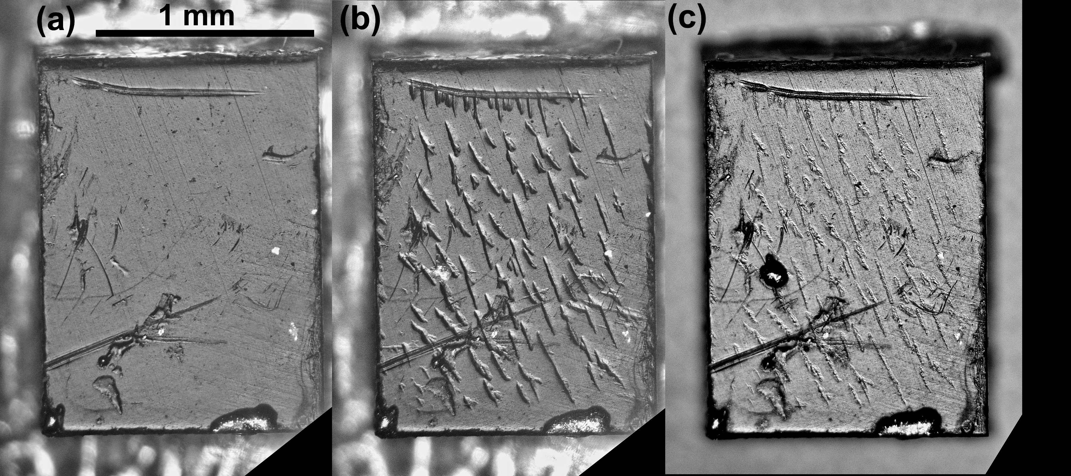
Figure 1: Polarized-light images of a [110] single crystal full of hydrogen. (a) room-temperature image of the crystal that was never cooled down; (b) the same crystal at 5 K showing profound hydrides outgrowths; (c) room temperature image of the crystal warmed after cooling showing scars - damage from the hydrides. These scars cannot be removed even by heating the sample to sub-melting temperatures indicating significant plastic deformation induced by the hydrides.

II Experimental

II.1 Samples

Seven niobium samples (four different types) were used in this work. Indeed, many samples of each type were measured during this study. The sample types are: (1,2) Two single crystals, both cut from the same large ingot and polished using water. They absorbed large amounts of hydrogen. (3) Commercial Nb foil from Alfa Aesar, 250 $\mu$m thick, 99.98% purity. It has been kept in a desiccator and showed no presence of hydrides. (4) Sputtered 160 nm thick niobium film, also kept dry and showing no obvious hydride formation. Identical films are used to make transmon qubits [39, 38]. (5,6,7) Samples cut out from different places of a real SRF cavity. A surface thermal map was constructed where surface temperature variations were measured in different spots during the resonance. In some places, called “hot spots” temperature rose by up to 1 K, whereas in other, called “cold spots”, changed only a little by 40 mK. Details of this mapping and measurements are found elsewhere [40]. All samples were cut and dry-polished down to sub-mm size to fit in our measurement setup.

II.2 London penetration depth

The London penetration depth was measured by using a sensitive tunnel diode resonator (TDR) technique [41, 42, 43, 44, 45, 46, 47]. Essentially, TDR is a tank circuit where the sample is inserted into a single-layer-of-turns inductor that produces a small, $H_{ac}<2~{}\text{$\mu$T}$, AC magnetic field at around $f_{0}\approx 14$ MHz. Connected in series tunnel diode, biased to the regime of negative differential resistance, compensates for losses in the circuit and for a certain impedance matching conditions, the circuit starts resonating spontaneously, usually below 70 K or so. If the diode and the circuit are well stabilized and isolated, the resolution of the device is about 1 part per billion resolving 0.01 Hz changes on top of 10 MHz main frequency. When a sample responds magnetically, the total inductance changes leading to a frequency shift, $\Delta f/f_{0}$, proportional to the samples magnetic susceptibility, $\chi\left(T\right)$, with a sample-dependent calibration constant, $\Delta f\left(T\right)/f_{0}=G\chi\left(T\right)$. The susceptibility may then be converted to the London penetration depth, using, $\left(1-N\right)\chi=\lambda/R\tanh\left(R/\lambda\right)-1$, knowing demagnetizing factor, $N$ [48], and the effective sample dimension, $R$ [47]. Since at low temperatures (practically below $0.8T_{c}$) the $\tanh$ term can be dropped and temperature dependence of the susceptibility analyzed since $\chi\left(T\right)\sim\lambda\left(T\right)$. Detailed description of the measurement procedure [43], calibration [42, 48, 47] and applications [44, 45, 46] provide a complete description of this unique technique capable of resolving sub-angstrom changes in the London penetration depth, $\lambda\left(T\right)$, in sub-mm sized crystals. Here we use it to study niobium samples from different sources.

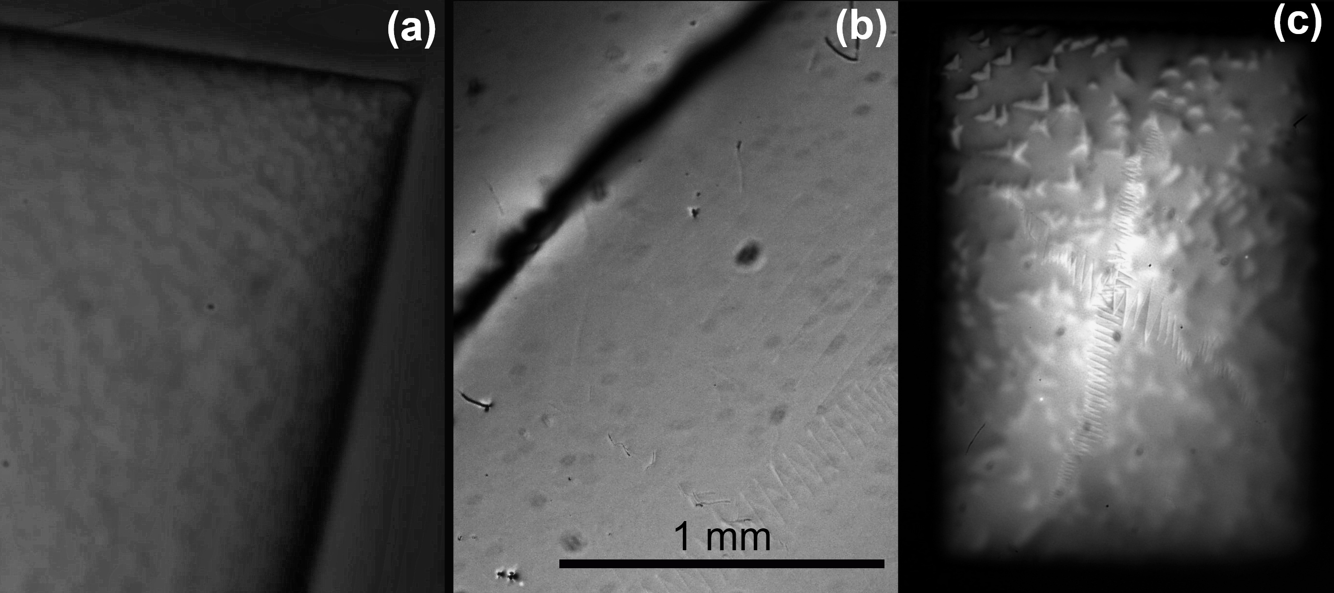
Figure 2: Magneto-optical Faraday images of three different cutouts from the SRF cavity. (a) cold spot from cavity’s inner surface showing small tubercles-like hydride structure; (b) a cutout 1 mm deep from cold spot showing no hydrides; (c) hot spot from the surface with characteristic boomerang-shaped large hydrides.

II.3 Low-temperature optical and magneto-optical imaging

The two-dimensional distribution of the magnetic induction was mapped in real-time employing magneto-optical imaging using Faraday effect in transparent ferrimagnetic indicators (bismuth-doped iron garnets) placed on top of the samples. Details of the technique can be found in our previous studies of Nb [49, 15]. The closed-cycle flow-type optical ⁴He cryostat exposed the cooled sample to an Olympus polarized-light microscope. The magnetic induction on the sample surface polarizes in-plane magnetic moments in the indicator, and the distribution of this polarization component along the light propagation is visualized through double Faraday rotation. In the images, only the magnetic field is visible due to a mirror sputtered at the bottom of the indicator.

The same microscope with the cryostat were used for direct observation in linearly polarized light. Due to polarization, all surface features become of higher contrast, because they often cause some rotation of the polarization plane upon reflection and since we work in (almost) crossed polarizer/analyzer configuration.

III Results and Discussion

III.1 Optical measurements

We start with optical characterization of the samples. Figure 1 shows polarized light imaging one of the [110] oriented (out of the page direction) single crystals cut from a big piece in presence of water, so it absorbed a significant amount of hydrogen. Panel (a) shows this crystal at the room temperature, never cooled down. No signature of surface features are seen. Panel (b) shows the same crystal at 5 K revealing large hydride formations. In our studies, we found that the hydrides tend to grow along principal directions and, therefore elongated shape here is not surprising. The direction, however, would depend on the strain, which is unknown. Figure 1(c) again shows a room-temperature image, but now after the cool-down. Scars left by the hydrides are clearly visible. These significant deformations and rapture of the previously perfect crystal would remain even if the crystal is heated up only few degrees below melting point of niobium. Therefore, the penetration depth data shown below were collected on a crystal full of large hydrides.

Next we examine three different cutouts from the SRF cavity. Two are from the inner surface and one from the depth of 1 mm beneath. Figure 2 shows magneto-optical images of each part in the remanent state of a trapped magnetic flux. (The sample is cooled in a magnetic field to low temperature and the field is turned off.) Importantly, sample surface is not visible, only trapped magnetic flux distribution. Figure 2 (a) shows the cold spot (where temperature variation did not exceed 40 mK). There are hydrides in shape of small tubercles. Panel (b) shows cutout from 1 mm depth under the cold spot revealing clean surface without the hydrides indicating that hydrogen distribution is highly non-uniform depth-wise. The third panel (c), shows a hot spot (temperature rose more than 1 K in a resonating cavity) revealing large hydrides similar to those observed in a single crystal, Fig.1.

We will now examine temperature-dependent superfluid density in these samples. This measurement brings information about the superconducting gap structure and possible pair-breaking mechanisms. In addition to crystals and cavity cutouts, we also measured a thin film used in the fabrication of transmons as well as commercial foil - to cover all possible states of niobium samples. Thin films from the same batches were characterized in great detail elsewhere [50].

III.2 London penetration depth

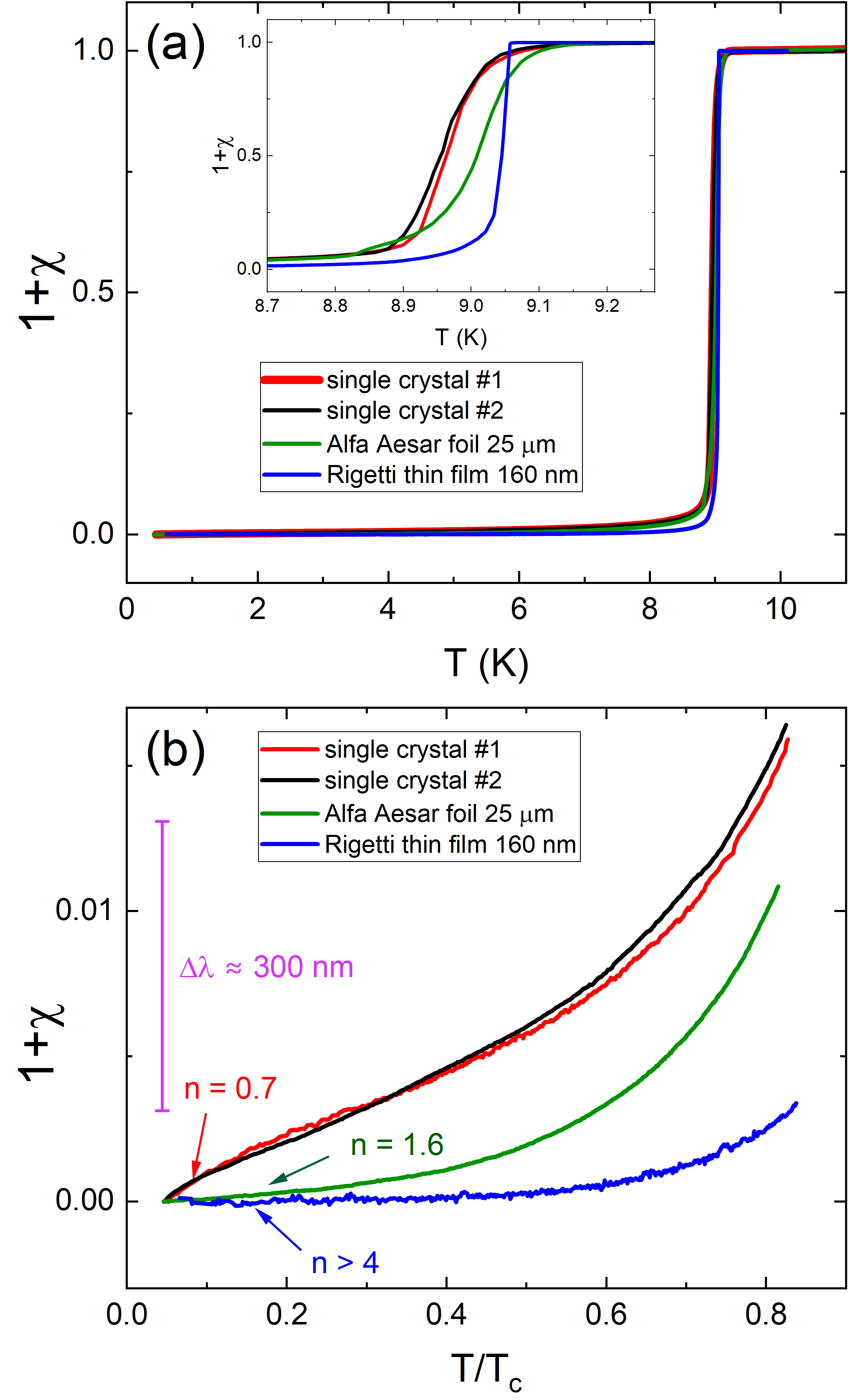
Figure 3: Magnetic susceptibility of two single crystals, Alfa Aesar foil and 160 nm Rigetti thin film. (a) main panel - full range, inset - zooming into the superconducting transition. (b) Low-temperature variation of London penetration depth fitted to the power-law, $\Delta\lambda\sim\left(T/T_{c}\right)^{n}$, from the base temperature, $0.044T_{c}$ to $0.3T_{c}$ yielding the values of the exponent $n$ indicated. Magenta bar show the corresponding scale of $\lambda\left(T\right)$ variation in nm.

The first set of measurements on two single crystals, Alfa Aesar foil and Rigetti thin film is shown in Fig.3. For comparison between different samples the curves were normalized to represent ideal magnetic susceptibility that starts at $\chi=0$ above $T_{c}$ and reaches $\chi=-1$ at the low temperature. The detailed shape of $\chi\left(T\right)$ is unaffected by this scaling. The inset in panel (a) of Fig.3 zooms at the superconducting transition showing the sharpest transition in Nb film and very similar $T_{c}$ in two crystals. All these values are somewhat lower than often quoted 9.3 K, likely due to disorder-induced pair-breaking in this quite anisotropic material [26, 51]. Figure 3(b) shows the low-temperature variation revealing quite different behaviors of $\lambda\left(T\right)$. The power-law fitting, $\Delta\lambda\sim\left(T/T_{c}\right)^{n}$ from the base temperature, $0.044T_{c}$ to $0.3T_{c}$ produced the indicated values of the exponent, $n$, which range from exponential attenuation, $n>4$, to a convex downturn with $n=0.7$, which is extremely unusual for any superconductor. In both single crystals we observe a downturn below roughly 1.3 K, whereas this behavior is absent in a thin film and a foil.

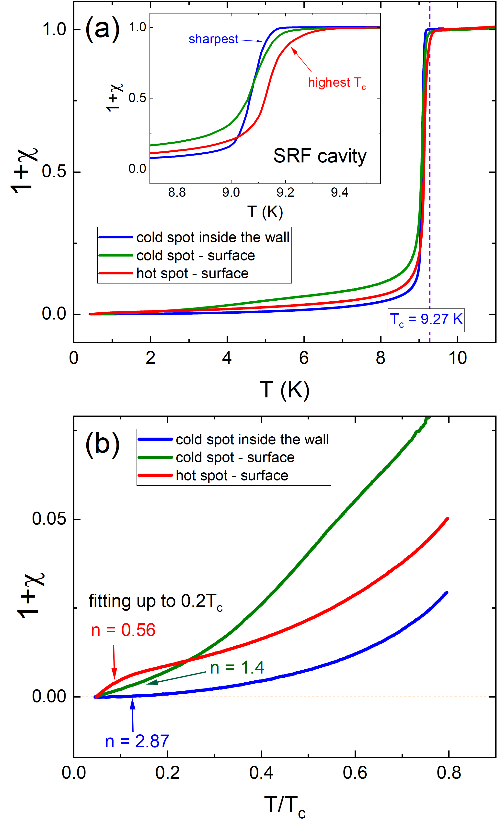
Figure 4: The information similar to Fig.3, but for the SRF cavity cutouts. Two from the surface, cold and hot spot, and the third from the depth of 1 mm under cold spot. While the transitions are higher, there is significant spread with widest transition width of about 0.4 K in the hot spot sample and the narrowest in the inner cold spot. (b) Low-temperature variation shows a distinct convex downturn, which is very unusual for $\lambda\left(T\right)$ in any superconductor. The inner cold spot shows saturation behavior consistent with a relatively clean superconducting gap.

The second set of data, shown in Fig.4, presents the results obtained in the SRF cavity cutouts in a way formally similar to the first set, Fig.3. Full temperature variation is presented in the main panel of Fig.4(a) and the inset zooms into the transition region. While the transitions are higher than in the first set, there is a more significant spread with the widest transition width of about 0.4 K in the hot spot sample and the narrowest in the inner cold spot. Panel (b) of Fig.4 presents low-temperature variation, showing even more pronounced downward curvature, but only for one sample that came from the cold spot. This fact will be the key for the interpretation of these results. Such distinct convex downturn is very unusual for $\lambda\left(T\right)$ in any (good and uniform) superconductor. The inner cold spot shows saturation behavior consistent with a relatively clean superconducting gap and the surface cold spot shows an intermediate behavior.

In principle, such behavior of the single crystals in Fig.3 and the hot spot sample in Fig.4 could be due to the proximity effect when superconductivity is induced in the surface metallic layer and the overall diamagnetic screening increases thus leading to the downturn in susceptibility. This was shown directly using TDR technique in MgB₂ wires that has excess magnesium on the surface [52]. Pambianchi et al. measured effective penetration depth in proximity-coupled Nb/Al bilayer films where they observed power law with exponent n$\leq$ 1 distinctly different from the exponential behavior of Nb [53]. However, in both works, the effect required a quite thick layer of another normal metal on niobium surface. It was suggested that niobium hydride phase, Nb₄H₃, which is also a candidate own superconductivity with a critical temperature of 1.2 K [54]. However, our niobium samples are exposed to air and poorly or non-conducting niobium oxides are formed on the surface thus eliminating the possibility of the formation of a good metallic layer. The oxides are very robust and withstand heating almost to melting temperature of Nb [35, 55]. Careful atom probe and transmission electron microscopy (TEM) studies showed no evidence of the metallic hydride phase on sample surfaces. In case of cavity cutouts, why would these layers only form over hot spots? Finally, the most important point is that proximity effect leads to the enhanced diamagnetism and the downturn is the departure from the original $\lambda(T)$ curve downward upon cooling. What we observe is opposite - the whole curve is shifted up indicating significant contamination of the superconducting gap with quasiparticle states rather than additional screening. Still, keeping in mind this possibility, we now turn to a more general analysis of the obtained results.

IV Theoretical analysis

IV.1 General remarks

Here we present a simple phenomenological analysis where we use a semiclassical connection between London penetration depth and the density of states. The results were verified by Matsubara summation formalism. Being phenomenological does not mean being qualitative. We use self-consistency equation to calculate the order parameter and then the superfluid density, and obtain quantitative prediction for temperature-dependent penetration depth. We follow the semiclassical approach introduced by Chandrasekhar et al. [56]. Some examples of using this theory for different superconductors can be found in Ref.[44]. The model gives direct connection between the superfluid density, $n_{s}\left(T\right)$, and the density of states, $N\left(E\right)/N_{n}$ normalized by its value at the Fermi level in the normal state, $N_{n}$. Here the energy of Bogolubov quasiparticles is, $E=\sqrt{\epsilon^{2}+\Delta^{2}}$ and the normal metal band energy, $\epsilon$, is measured from the Fermi level. The response of supercurrent to a vector potential, $\mathbf{J=\mathbb{-R}A}$, is determined by the so-called response tensor, $\mathbb{R}$, which consists of two parts, diamagnetic and paramagnetic. The full expression involves the average over the Fermi surface of a possibly anisotropic gap function. In case of niobium we can safely use spherical Fermi surface and constant gap (although the gap is somewhat anisotropic [26]. Then the superfluid density, normalized on its value in the clean case (which is the total electron density of normal metal), reads:

$$n_{s}=1+2\intop_{0}^{\infty}\frac{\partial f\left(E\right)}{\partial E}\frac{N\left(E\right)}{N_{n}}dE$$ (1)

where the order parameter enters the density of states as,

$$\frac{N\left(E\right)}{N_{n}}=\frac{E}{\sqrt{E^{2}-\Delta^{2}}}$$ (2)

The derivative of the Fermi function is,

$$\frac{\partial f\left(E\right)}{\partial E}=-\frac{1}{4t}\text{sech}^{2}\left(\frac{E}{2t}\right)$$ (3)

where $t=T/T_{c}$ (note that this is actual superconducting transition temperature that may be lower than the “clean” value that we denote $T_{c0}$) and quasiparticle energy is dimensionless in units of $k_{B}T_{c}$ and we set $k_{B}=1$ everywhere. The quantity of interest, the London penetration depth is then obtained from Eq.1 as,

$$\frac{\lambda\left(T\right)}{\lambda_{0}}=\frac{1}{\sqrt{n_{s}}}$$ (4)

where $\lambda_{0}$ is a clean-limit London penetration depth. Therefore, with scattering, this ratio will be greater than 1 even at $T=0$.

Importantly, this approach does not specify how the order parameter is obtained. In the original papers of the semiclassical approach where very clean superconductors were considered [57], it was sufficient to use the so-called Einzel ansatz to analytically represent the gap with high accuracy [58]. This is insufficient for our purposes as we would like to explore “contaminated” gaps, thus we will use the self-consistent solutions for $\Delta\left(T,\Gamma\right)$, where $\Gamma$ is pair-breaking scattering rate [21].

IV.2 Dynes superconductors

The simplest way to introduce pair-breaking into the density of states is to consider Dynes superconductors. There are several comprehensive works with a detailed analysis of the Dynes model and its applicability to realistic and quite complicated cases. A full set of all thermodynamic and transport parameters was calculated and is available for reference. We follow to extensive coverage of the Dynes model by Gurevich and Kubo [59, 60, 61, 62] and Herman and Hlubina [63, 64, 65]. In this model, instead of Eq.2, the density of states is given by,

$$\frac{N\left(E\right)}{N_{n}}=\Re\left[\frac{E+i\Gamma}{\sqrt{\left(E+i\Gamma\right)^{2}-\Delta^{2}}}\right]$$ (5)

Dynes superconductors are gapless. At $E=0$, Eq.5 gives $N\left(E\right)=N_{n}\Gamma/\sqrt{\Gamma^{2}+\Delta^{2}}$. However, for small rates (usually found in tunneling experiments [66, 55]), $\Gamma\ll\Delta$, one obtains quite useful estimates. In general the meaning of this phenomenological parameter is that $\hbar/\Gamma$ is the quasiparticle lifetime. It also has meaning of pair-breaking scattering time, because Dynes $\Gamma$ is analogous to Abrikosov-Gor’kov (AG) scattering parameter [67],

$$\rho=\frac{\hbar}{2\pi T_{c}\tau}=\frac{\Gamma}{2\pi}$$ (6)

(actually, in the original paper, AG used $\rho$ without “2” in the denominator), and the $T_{c}$ for Dynes superconductor is obtained from a classical AG formula [60],

$$\psi\left(\frac{\Gamma}{2\pi t_{c}}+\frac{1}{2}\right)-\psi\left(\frac{1}{2}\right)+\ln\left(t_{c}\right)=0$$ (7)

where $t_{c}=T_{c}/T_{c0}$ and $\psi\left(x\right)$ is digamma function. The transition temperature becomes zero when $\Gamma_{crit}=0.8819$.

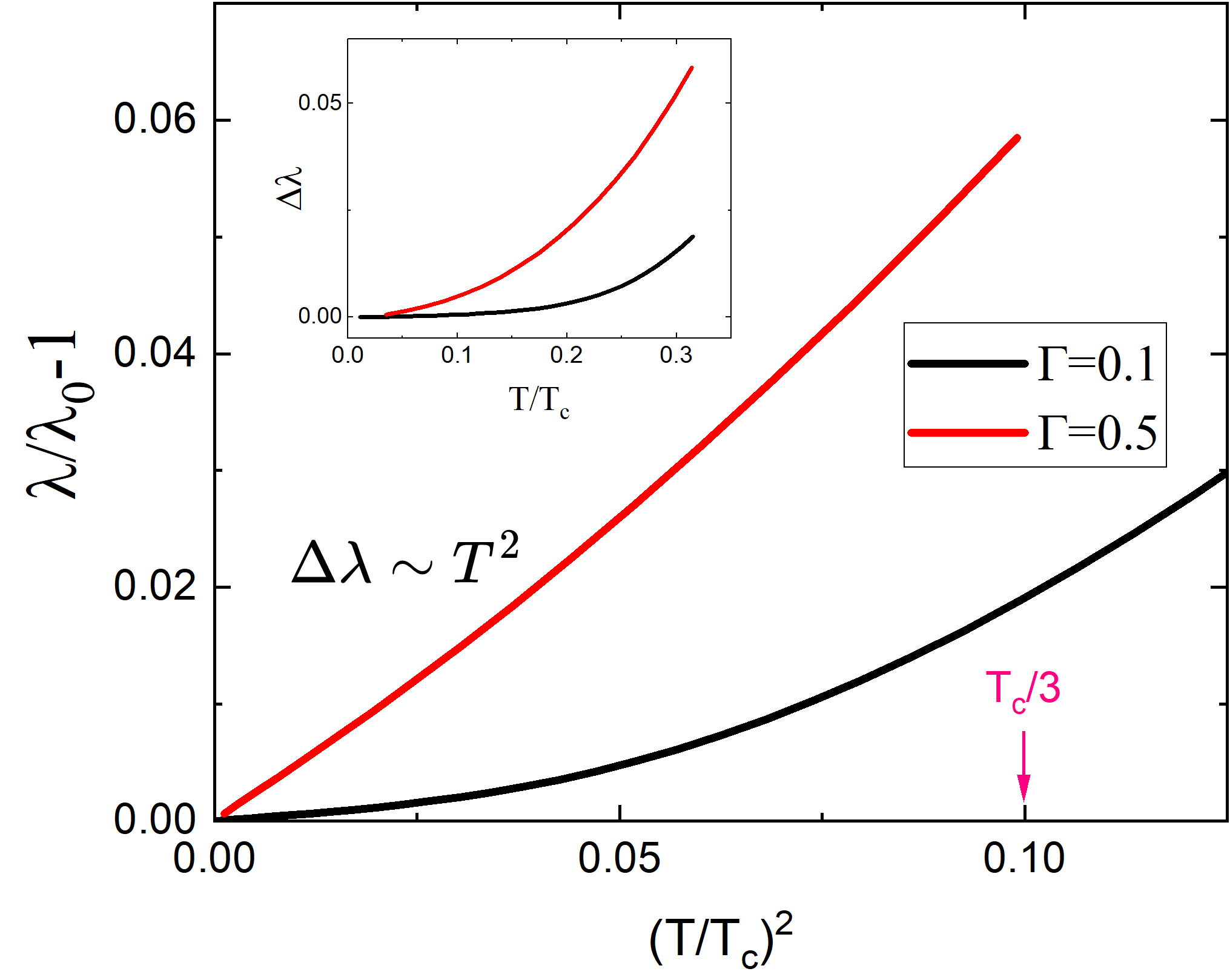
Figure 5: The change of the London penetration depth, calculated using Eqs. 8,5,1 and 4. (Here we put $\lambda_{0}=1$). At larger scattering rates it approaches quadratic temperature dependence as predicted by Gurevich and Kubo [68].

To calculate the superfluid density, we need to solve the self-consistency equation for the order parameter written in terms of Matsubara sum [60],

$$\log(t)-\sum_{n=0}^{n_{max}}\left(\frac{2\pi t}{\sqrt{\Delta^{2}+\left(\Gamma+2\pi t\left(n+\frac{1}{2}\right)\right)^{2}}}-\frac{2}{2n+1}\right)=0$$ (8)

For each value of $\Gamma$ and for each temperature, $t$, Eq.8 yields $\Delta\left(t,\Gamma\right)$. The number of terms, $n_{max}$ depends on the required accuracy and the lower the temperature, the more terms are needed. Here we used $n_{max}=10000$.

Now we are set to calculate the London penetration depth as function of temperature for different values of $\Gamma$ and compare with the experiment. One difficulty is that the formulation in form of Eq.1 does not include the effect of pair-conserving scattering, which nevertheless affects the superfluid density. For Dynes superconductor this is solved by calculating superfluid density using Matsubara sum as introduced by Herman and Hlubina [64],

$$n_{s}=2\pi t\sum_{n=0}^{n_{max}}\frac{\Delta^{2}}{\Omega_{n}^{2}(\Omega_{n}+\Gamma_{s})}$$ (9)

where $\Omega_{n}=\sqrt{\Delta^{2}+(\Gamma+\pi t(2n+1))^{2}}$. Here two scattering parameters are present, the pair-breaking $\Gamma$ that also enters the original Dynes equation, Eq.5 and pair-conserving scattering rate, $\Gamma_{s}$.

Figure 5 shows the variation of the London penetration depth, calculated using Eqs. 8,5,1 and 4. (Here $\lambda_{0}=1$). Identical results are obtained from Eq.9 with $\Gamma_{s}=0$. At fairly small rates, the behavior is sub-quadratic, but clearly non-exponential indicating significant deviation from the clean (exponential) case. At larger scattering rates penetration depth approaches quadratic temperature dependence as predicted by Gurevich and Kubo [68]. Compared with our experimental results, such behavior would be consistent with the Alfa Aesar foil, Fig.3 and, perhaps to some extend with the cold spot shown in Fig.4.

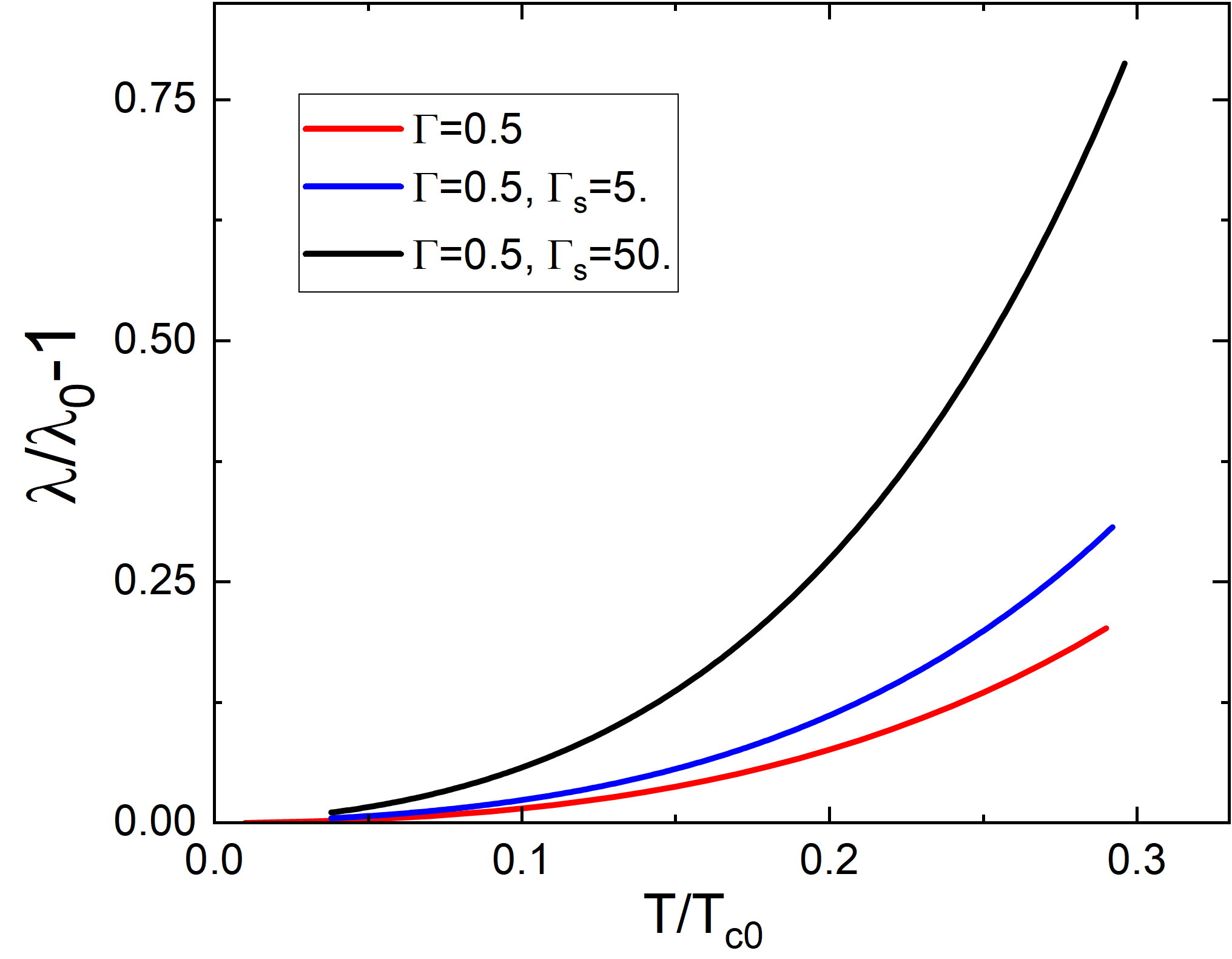
Figure 6: Temperature dependent London penetration depth, $\Delta\lambda(T)$, calculated for a fixed Dyson pair-breaking $\Gamma=0.5$ and $\Gamma_{s}=0,5,50$. While, expectedly, the slope becomes steeper, the behavior remains close to quadratic (note that, unlike Fig.5, this is linear scale.)

Still, we are not even close to reproducing the downturn. Perhaps, pair-conserving $\Gamma_{s}$ will help? Figure 6 shows penetration depth for a fixed Dyson pair-breaking, $\Gamma=0.5$, and pair-conserving, $\Gamma_{s}=0,5,50$ (unlike $\Gamma$, the pair-conserving $\Gamma_{s}$ can assume any values, but dirty behavior starts with the values above 1, so 50 is an exaggeration to see the difference. While the temperature variation became much steeper, the functional form remains sub-quadratic. To explore other possibilities we turn to the two-level systems.

IV.3 Two-level systems and penetration depth

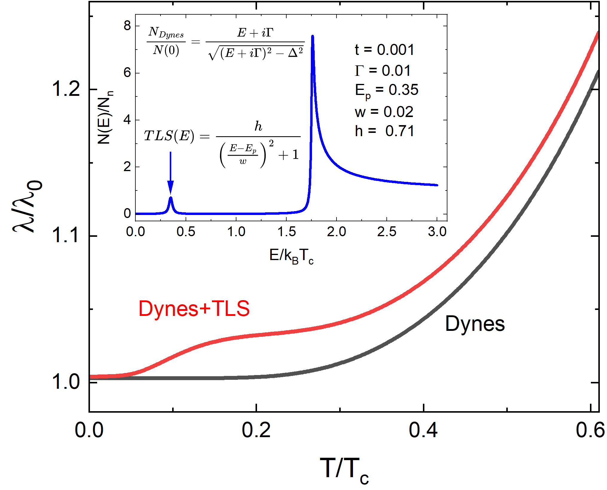
Figure 7: Temperature dependent London penetration depth, calculated using Eq.1 with (red line) and without (black line) TLS contribution to the density of states. The total $N\left(E\right)/N_{n}$ is shown in the inset. A relatively small peak, with the parameters indicated, causes such a dramatic change in the penetration depth. Importantly, it naturally produces the downturn in the penetration depth.

There is a significant interest in TLS, which are intensely studied theoretically and experimentally. Here we are only interested in their possible effect on the London penetration depth. For that, it is sufficient to model TLS as small peaks deep inside the superconducting energy gap in the density of states. Since the superfluid density is the integral over all energies, we do not think the precise details of the TLS peak may drastically change the outcome. Here we model the TLS density of states as a Lorentzian,

$$TLS(E)=\frac{h}{\left(\frac{E-E_{p}}{w}\right)^{2}+1}$$ (10)

so that this peak of height $h$ and width $w$ is located at energy $E_{p}$ inside the Dynes gap. An example is shown in the inset in Fig.7. The total DOS is obtained by adding Eq.5 and Eq.10. Then Eq.1 is used to calculate the superfluid density shown in Fig.8. The black curves on both figures are the results for Dynes superconductor with small $\Gamma=0.01$ showing close to isotropic s-wave BCS classical exponential attenuation at low temperatures. The introduction of a small TLS peak changes situation drastically. This is because its location deep inside the gap. According to Eq.1, the reduction of the superfluid density is proportional to the product of DOS and derivative of the Fermi function. The latter is steep at low temperatures and when it reaches even a small peak, the result is significant.

Clearly, this mechanism naturally explains our observations of the downturn in the penetration depth. While the hydrides are clearly not good for applications because they increase overall surface impedance and lead to significant dissipation, the downturn is not their signature. Further research is needed to clarify the nature of TLS which is much more complicated than used here and involved dynamic processes, we believe our measurements and analysis presented a complimentary way to identify TLS in niobium based applications.

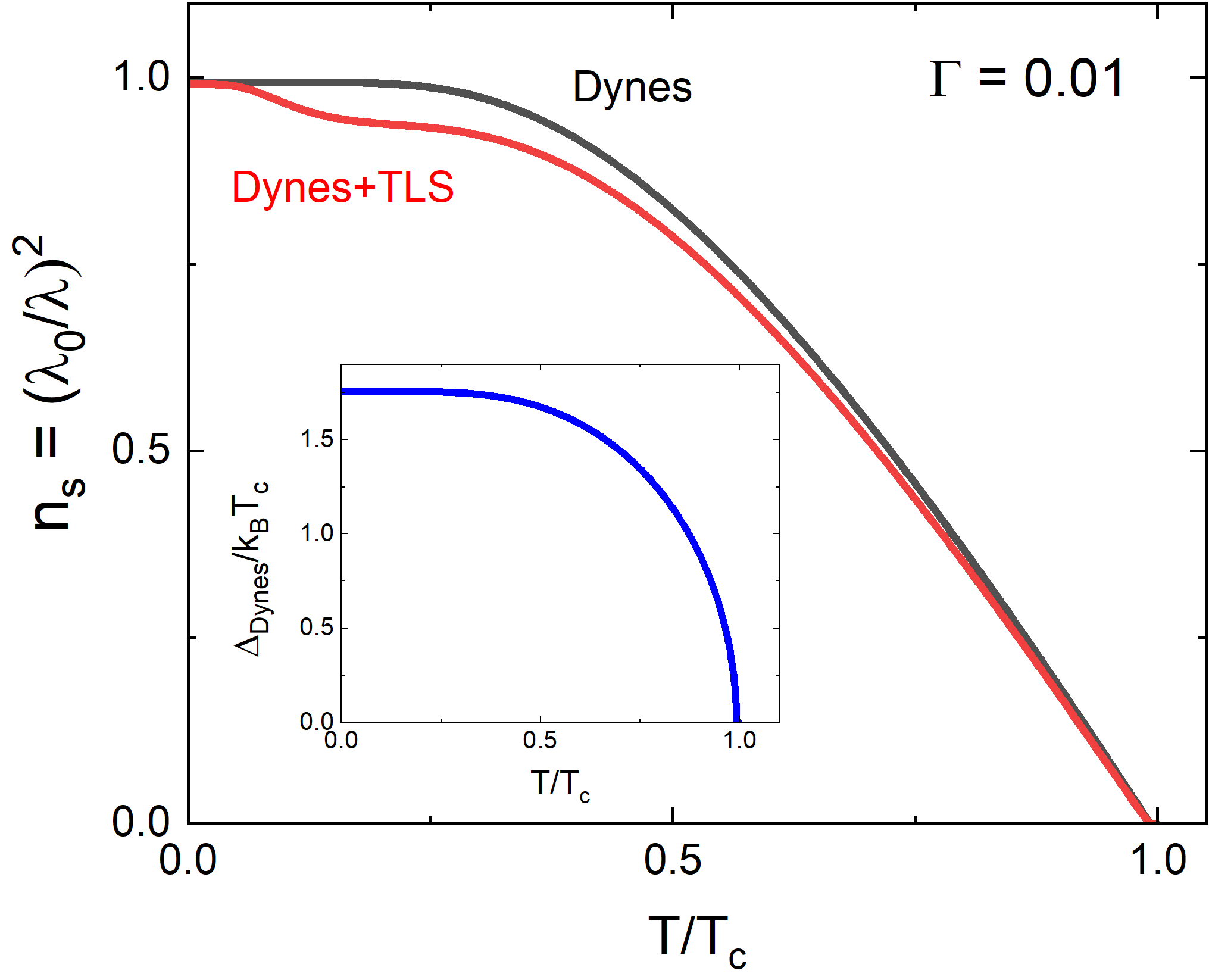
Figure 8: Temperature dependent superfluid density with and without TLS. The Dynes curve was computed for small $\Gamma=0.01$ and the TLS parameters are shown in the inset in Fig.7. A pronounced depression at low temperatures may explain various issues appearing upon deep cooling. Inset shows self-consistent order parameter as function of temperature.

V Conclusions

Dyson pair-breaking $\Gamma$ changes temperature variation from exponential to the power law, but not faster than quadratic behavior. The pair-conserving $\Gamma_{s}$ only increases the rate of change, but does not significantly alter the functional form of $\lambda(T)$. The two-level systems residing inside the gap have profound effect changing exponential attenuation to sub-linear downward concave curvature of $\lambda(T)$. We emphasize that this was a limited study designed to probe a variety of different types of samples. Systematic measurements of each type are needed to identify the actual cause behind the TLS-like behavior.