Classical time crystal Ginzburg-Landau study of coupled parametric oscillators

Abstract

Discrete time crystals, which are phases of matter that break the discrete time translational symmetry of a periodically driven system, have generated a wave of recent interest and activity. In this work, we propose a classical system of weakly nonlinear parametrically driven coupled oscillators as a testbed to understand these phases. Such a system of oscillators in the presence of dissipation has a period-doubling instability only at long wavelengths where a large number of oscillators are in phase. To show that this instability leads to a discrete time crystal when exposed to noise and non-linearity, we derive a general condition to predict when a Markov process will break time-translation symmetry. The first requirement of this condition is that the Markov chain over doubled time steps has a stationary probability distribution that spontaneously breaks a local symmetry. The second requirement is that the order parameter flips sign over a single time step. We show that our system of oscillators features period-doubling and yields a stationary probability distribution given by a spatially continuous Ginzburg-Landau Hamiltonian with spontaneous symmetry breaking. We then discuss applications of the general condition to existing time crystal platforms.

I Introduction

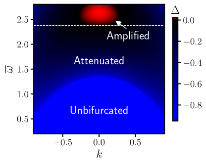
Figure 1: Total gain $\Delta$ after one period $T$ of a coupled array of parametrically driven linear oscillators as a function of momentum $k$ and average natural frequency $\overline{\omega}\equiv(\omega_{1}+\omega_{2})/2$. The time-period of the parametric drive is $T=1$ and the oscillators are damped with a constant $\Gamma=1.9$. The gain is given explicitly by $\Delta=\log|\lambda_{k}|-\Gamma T/2$, where $\lambda_{k}$ is the largest Floquet eigenvalue of the oscillator by magnitude (see Eq. 6). All bifurcated points are in the period-doubled regime, i.e. $\lambda_{k}<0$. The horizontal dashed line corresponds to the point where the damping is critical, i.e. $\Gamma=\Gamma_{c}=(2/T)\log|\lambda_{k=0}|$. $J=10$, $|\omega_{1}-\omega_{2}|/2=0.664\pi$.

While the spontaneous breaking of physical symmetries forms a cornerstone of our understanding of phases of matter, the breaking of time-translation invariance has lacked an obvious example until relatively recently. The past several years have seen new proposals [1, 2, 3] for possible candidates, dubbed “time-crystals” owing to their spatial analogs, which feature an emergent periodicity with an infinite autocorrelation time at finite temperature. Shortly after the initial proposal, two no-go theorems [4, 5] demonstrated that the breaking of a continuous time-translation symmetry cannot be robust to noise and therefore cannot host time crystal phases. Current work therefore focuses on “discrete time crystals” (DTCs) in driven Floquet systems which reduce a time-translation symmetry group $\mathbbm{Z}$ to a subgroup $n\mathbbm{Z}$ [3, 6, 7, 8, 9, 10, 11].

The presence of an external drive in a closed system leads to constraints associated with ergodicity since ergodic systems will heat to infinite temperature [12, 13, 14]. Disorder and many-body localization in closed quantum systems may provide one way to avoid these loopholes and provide the possibility of dynamical symmetry breaking in an infinite temperature phase [15, 16, 17, 8, 3, 7, 9]. Other routes to avoid thermalization include high frequency drives in classical Hamiltonian systems [18, 19, 19, 20, 21, 22, 23] or even more simply, Floquet systems with dissipation, which can be either quantum or classical. This last platform has inspired recent theoretical [24, 25, 26, 27, 23] and experimental [28, 29, 30, 31, 32, 33, 34, 35, 36, 37, 38] works.

Examples of DTC order in classical systems have been termed classical discrete time crystal (CDTC) and appear in the modern context in coupled arrays of nonlinear pendula (i.e. the so-called parametrically driven periodic Frenkel-Kontorova model) [39]. While such a CDTC behavior might appear to be reminiscent of subharmonic entrainment in classical mechanics [40, 41], the latter is traditionally discussed with regard to noise-free dynamical systems and therefore does not apply to the discussion of a phase. The robustness to noise indicative of a phase [42] likely requires an extended system to allow for the concept of a thermodynamic limit, avoiding ergodicity constraints of local random dynamics [39]. While several examples of subharmonic entrainment have been studied experimentally and numerically in extended solid state systems [43, 44], the result of a stable phase in a noisy [45], extended model has not been explored until recently.

More abstractly, Markovian update rules can describe noisy dissipative systems which, with local interactions, take the form of probabilistic cellular automata (PCA). Recent studies of such PCA systems find “prethermal states” which are robust for exponentially long times but lack the true infinite autocorrelation of a time crystal [46, 47, 48, 49, 50]. However a few decades ago, Gács and Toom showed a remarkable counter-example to ergodicity in PCAs, qualifying as a true CDTC [51, 52, 53, 11]. In fact, these phases are remarkable in that they show spontaneous symmetry breaking (SSB) in one dimension with short-ranged interactions, which cannot happen for Hamiltonian systems. On the contrary, in analogy with the dynamics of SSB in equilibrium systems [54, 55], one can expect a intermediate possibility where the correlation time of the period-doubling order is finite but exponentially large in the system size. We will refer to this phenomenon as a CDTC as opposed to prethermal.

In this work we consider an array of parametrically driven oscillators as a platform to study a CDTC phase. As shown in Fig. 1 and detailed in Sec. II, for an appropriate choice of the average natural frequency (or spring constant), the array of oscillators shows a period-doubling amplifying phase over a small range of wave-vectors $k$. This array of oscillators amplifies a mode with a period $2T$, which is exactly double the period $T$ of the drive near wave-vector $k\sim 0$. Introducing dissipation to nearly cancel the parametric amplification and only considering snapshots at periods $2T$, we can approximate the dynamics as smooth in space and time.

In Sec. III, we take advantage of this smoothness to show that this exponential instability can be converted into a symmetry breaking phase transition by the combination of nonlinearity and noise. This demonstration relies on a mapping from the period-doubled CDTC phase to the ordered phase of a Ginzburg-Landau Hamiltonian. While analytically tractable, this analysis relies on an expansion of small nonlinearity and noise corresponding to low temperatures. In Sec. III.1 we use the known results of Ising transitions to show that our analysis predicts ordered phases for oscillators coupled by power-law ranged interactions similar to the PCA analysis [56, 46]. In Sec. IV, we argue using general properties of Markov chains that the CDTC order, with a correlation time that scales exponentially in system size, should continue to apply over a finite range of $\epsilon$.

II Period-doubling in coupled parametric amplifiers

We start by considering a coupled array of parametric oscillators [57] with translational invariance in arbitrary dimensions. Such a system can be described by a time-dependent Hamiltonian

$$H(t) =\sum_{j}\frac{1}{2}\dot{\phi}_{j}^{2}+\frac{1}{2}\omega_{0}^{2}(t)\phi_{j}^{2}+\frac{J}{2}\left(\phi_{j}-\phi_{j+1}\right)^{2}.$$ (1)

Spatial translation invariance allows us to decouple the oscillators into independent Bloch momentum modes, represented as vectors in phase space $\psi_{k}=(\phi_{k},\dot{\phi}_{k})^{T}$. Allowing for the possibility of a damping $\Gamma$ to each oscillator, the equation of motion of the Fourier component $\phi_{k}(t)$ is written as $\ddot{\phi}_{k}=-\left[\omega_{0}^{2}(t)+2J\sin^{2}\left(k/2\right)\right]\phi_{k}-\Gamma\dot{\phi}_{k}$. We factor out this damping by defining $\tilde{\phi}_{k}\equiv e^{\Gamma t/2}\phi_{k}$ such that the damping term can be eliminated from the equation of motion

$$\ddot{\tilde{\phi}}_{k}=-\Omega_{k}^{2}(t)\,\tilde{\phi}_{k},$$ (2)

where

$$\Omega_{k}^{2}(t)\equiv\omega_{0}^{2}(t)+2J\sin^{2}\left(k/2\right)-{(\Gamma/2)}^{2}.$$ (3)

We can also relate the two-component phase-space vector $\psi_{k}$ to its damped counterpart $\tilde{\psi}_{k}$ using the transformation $\tilde{\psi}_{k}=P_{\Gamma}e^{\Gamma t/2}\psi_{k}$ where $P_{\Gamma}\equiv\left(\begin{smallmatrix}1&0\\ \Gamma/2&1\end{smallmatrix}\right)$.

To understand the dynamics using Floquet analysis [58], we describe the motion over one driving period with the transfer matrix $M_{k}$ such that $\psi_{k}(T)=M_{k}\psi_{k}(0)$, or $\tilde{\psi}_{k}(T)=\tilde{M}_{k}\tilde{\psi}_{k}(0)$ for the damped phase space vector. In the case where $\omega_{0}(t)$ is time-independent, $M_{k}$ is effectively unitary (i.e. with eigenvalues of unit magnitude) and the modes preserve their amplitude in a way to conserve the energy. More interesting behavior can be obtained when $\omega_{0}(t)$ is parametrically time-dependent at a driving frequency around half of the natural frequency. Such a driven oscillator leads to parametric resonance [57] featuring “amplified” and “squeezed” modes.

For the purpose of illustration, we consider a general piecewise-constant time dependence of the driving frequency

$$\quad\omega_{0}(t)=\begin{cases}\omega_{1}&\left\{\frac{t}{T}\right\}<\frac{1}{2}\\ \omega_{2}&\left\{\frac{t}{T}\right\}\geq\frac{1}{2}\end{cases},$$ (4)

where curly brackets denote the fractional part. Since the corresponding frequency $\Omega_{k}(t)$ is also piecewise constant in time, we abbreviate its values as $\Omega_{k,j}$ where $j=1,2$ following Eq. 4. We then calculate the total transfer matrix $\tilde{M}_{k}$ as the product of two transfer matrices $\tilde{M}_{k}=\tilde{M}_{k,2}(T/2)\,\tilde{M}_{k,1}(T/2)$ where $\tilde{M}_{k,j}$ is the transfer matrix over the time-independent regions of the drive:

$$\tilde{M}_{k,j}(t) =\exp\left[\left(\begin{matrix}0&1\\ -\Omega_{k,j}^{2}&0\end{matrix}\right)t\right].$$ (5)

Since $\tilde{M}_{k}$ has determinant 1, its trace is $\tr\tilde{M}_{k}=\lambda_{k}+\lambda_{k}^{-1}$ where $\lambda_{k}$ and $\lambda_{k}^{-1}$ are the eigenvalues of $\tilde{M}_{k}$. Assuming without loss of generality that $|\lambda_{k}|\geq 1$, the parametric oscillator at wave-vector $k$ demonstrates amplifying behavior when $|\lambda_{k}|>1$. Since $\tilde{M}_{k}$ is real, and $|\lambda_{k}|\neq|\lambda_{k}^{-1}|$, the eigenvalue $\lambda_{k}$ must be real. The driven oscillator then displays a parametric resonance when $|\tr\tilde{M}_{k}|>2$.

The parametric amplification can lead to an instability towards a period-doubled state when $\tr\tilde{M}_{k}<-2$ since in this case, the eigenvalues $\lambda_{k}$ are negative real numbers. As a result the parametrically amplified normal mode $\psi^{A}_{k}(t)$, as well as the corresponding displacement $\phi_{k}^{A}(t)$, switches sign between periods:

$$\psi^{A}_{k}(T) =P_{\Gamma}^{-1}e^{-\Gamma T/2}\tilde{M}_{k}P_{\Gamma}\psi^{A}_{k}(0)$$

$$=\lambda_{k}e^{-\Gamma T/2}\psi^{A}_{k}(0)$$

$$=-|\lambda_{k}e^{-\Gamma T/2}|\psi^{A}_{k}(0).$$ (6)

Such a period-doubling parametric amplification at wave-vector $k$ occurs when the parameters $\Omega_{k,j}$ satisfy

$$\delta\Omega_{k}^{2}\cos\delta\Omega_{k}-\overline{\Omega}_{k}^{2}\cos\overline{\Omega}_{k}>\Omega_{k,1}\Omega_{k,2}$$ (7)

where $\overline{\Omega}_{k}=(\Omega_{k,1}+\Omega_{k,2})/2$ and $\delta\Omega_{k}=(\Omega_{k,1}-\Omega_{k,2})/2$, scaling the driving period to $T=1$.

As shown in Appendix A, our choice of $\Omega_{k,j}$ resulting from Eq. 3 and Eq. 4 maximizes the period-doubling parametric amplification eigenvalue $|\lambda_{k}e^{-\Gamma T/2}|$ at $k=0$. Thus, if we choose a critical damping $\Gamma_{c}$ such that $\Gamma_{c}T/2=\log\lambda_{k=0}-\epsilon$, where $\epsilon>0$ is an infinitesimally small parameter, the coupled system of parametric oscillators described by Eq. 1 together with damping shows period-doubling amplification at $k=0$. Physically, this means that each oscillator $\phi_{j}(t)$ satisfies the period-doubling condition $\phi_{j}(T)=-\phi_{j}(0)$ for all lattice sites $j$. This state of the coupled parametric oscillator, starting from any initial displacement, becomes a steady state of all oscillators where the $k=0$ parametric amplified state takes over i.e.

$$\phi_{j}(nT)\rightarrow(-1)^{n}(1+\epsilon)^{n}\phi(0),$$ (8)

as $n\rightarrow\infty$ where $\phi(0)$ is an initial amplitude, which is slowly amplified for $\epsilon>0$. Fig. 1 shows the range of wave-vectors $k$ over which such amplification occurs as a function of average natural frequency for specific optimal parameters (detailed in Appendix A). In addition to the amplified region, the figure shows a unbifurcated region where the modes are related by complex conjugation and show periodic dynamics at a frequency near the average natural frequency. These modes are attenuated at the rate of the externally imposed damping, without which the dynamics would be equivalent to a simple harmonic oscillator. Since the results in the figure are for a system with a finite amount of damping, the figure also supports an attenuated region in addition to the amplified and unbifurcated region. This region is characterized by dynamics that is attenuated at a rate slower than the externally imposed damping. In fact, in the absence of such damping, the amplified region would expand to include all of the attenuated range.

This state in the fine-tuned limit of $\epsilon=0$ reaches an exact period-doubled steady state, exhibiting subharmonic entrainment. However, this does not satisfy the robustness criteria of a CDTC since it is sensitive to changes in $\Gamma$ or other parameters of the system. Furthermore, the dynamics of this state is in some sense critical; i.e. it takes a divergent amount of time for the system to approach the period-doubled state. However, as we will show in the next section, the addition of weak noise and anharmonicity can stabilize this state into a CDTC.

III Stabilizing the Period-Doubled State with Noise and Nonlinearity

To study the emergence and robustness of this period-doubled phase, we set the damping to $\Gamma=\Gamma_{c}-\nu\epsilon/T$ ($\nu$ is a constant factor which we add for later convenience) and introduce a restoring nonlinear force proportional to $\epsilon$, stabilizing the mode at a fixed point which is independent of $\epsilon$. Finally, we introduce Gaussian noise to the system, also proportional to the infinitesimal $\epsilon$. The force

$$f_{k}(t) =\epsilon\sum_{j}e^{-ikx}\left[-g\phi_{j}(t)^{3}+\frac{\nu}{T}\dot{\phi}_{j}(t)+W_{j}(t)\right].$$ (9)

combines these three perturbations. Here $g$ is the relative strength of the nonlinear force and $W_{j}(t)$ is uncorrelated Gaussian white noise with variance $\langle W_{i}(t)W_{j}(t^{\prime})\rangle=2D_{m}\delta_{ij}\delta(t-t^{\prime})$.

In what follows, we will understand the effect of the perturbatively small (i.e. of order $\epsilon$) nonlinear force $f_{k}(t)$ by ultimately mapping to a time-dependent Ginzburg-Landau model [59] using coarse-grained dynamics in space and time. The parametric instability of the linear model at $k\sim 0$ is conducive to such a treatment because the amplified fluctuations would be smooth in space. However, the period-doubled state, where the displacement flips sign every period $T$ presents a challenge to such a treatment. This issue can be circumvented by considering the dynamics at even time-steps i.e. $t=2nT$. Therefore, the dynamics of the parametric amplifier $\psi_{j}(2nT)$ in the last section can be approximated as a smooth slowly varying field in position $j$ and time $n$. Taking the Fourier transform of the spatial dependence $j$ to momentum $k$, we can write the coarse-grained equation of motion for $\psi_{k}(2nT)$ using Green functions as

$$\psi_{k}(2nT) =\left(1+\nu\epsilon\right)^{n}M_{k}^{2n}\psi_{k}(0)$$

$$+\epsilon\int_{0}^{2nT}d\tau\,G_{k}(2nT,\tau)e_{2}F_{k}[\{\psi_{k}\},\tau]$$

$$+\epsilon\int_{0}^{2nT}d\tau\,G_{k}(2nT,\tau)e_{2}W_{k}(\tau).$$ (10)

where

$$F_{k}[\{\psi_{k}\},\tau]\equiv-g\int dk_{1,2}\phi_{k_{1}}(\tau)\phi_{k_{2}}(\tau)\phi_{k-k_{1}-k_{2}}(\tau).$$ (11)

For sufficiently large $n$, the squeezed eigenvalue of $M_{k}^{2n}$ becomes comparable to $\epsilon$ for all momenta. Since the other terms in Eq. 10 also include factors of $\epsilon$, the total amplitude of the squeezed mode at long times from the initial state must be on the order of $\epsilon$. The squeezed mode’s effect on the amplified mode via the nonlinearity is then proportional to $\epsilon^{2}$ and we can safely ignore its contribution to understand the steady state dynamics of the amplified mode. Using this assumption and considering the dynamics of the amplified mode over a time interval of length $2T$ in the steady state, we can write the equations of motion of a single component which describes overdamped dynamics as:

$$\psi^{A}_{k}(2T) =\left(1+\nu\epsilon\right)\lambda_{k}^{2}\psi^{A}_{k}(0)+\epsilon\eta_{k}$$

$$-\epsilon g\int dk_{1,2}\,\zeta_{k,k_{1},k_{2}}\,\phi^{A}_{k_{1}}(0)\phi^{A}_{k_{2}}(0)\phi^{A}_{k-k_{1}-k_{2}}(0).$$

The factors $\zeta_{k,k_{1},k_{2}}$ and $\eta_{k}$ encode the nonlinear propagation and stochastic process over two driving periods, given explicitly in Eqs. 33.

Since we are considering a system in the thermodynamics limit, the momenta are effectively continuous and we can rescale $k\rightarrow k\sqrt{\epsilon}$. This allows us to expand the amplification rate as

$$(1+\nu\epsilon)\lambda_{k}^{2}=(1+\nu\epsilon)-\epsilon\gamma k^{2}+O(\epsilon^{2}).$$

Furthermore, the coefficient for the nonlinear term and the noise strength both become $k$-independent up to leading order in $\epsilon$, allowing us to replace $\zeta_{k,k_{1},k_{2}}$ with $\zeta\equiv\zeta_{0,0,0}$ and define the variance of $\eta_{k}$ to be $2D$ (see Eq. 34).

In this picture, the oscillations disappear leaving only overdamped, slow dynamics. Motivated by the time derivative in the Langevin equation, we compute the finite difference in $\phi^{A}_{k}$ over one period, pulling the value $\epsilon$ to the left-hand side:

$$\frac{\phi^{A}_{k}(2T)-\phi^{A}_{k}(0)}{\epsilon} =\nu\phi^{A}_{k}(0)-\frac{\gamma}{2}k^{2}\phi^{A}_{k}(0)+\eta_{k}$$

$$-g\zeta\int dk_{1,2}\,\phi^{A}_{k_{1}}(0)\phi^{A}_{k_{2}}(0)\phi^{A}_{k-k_{1}-k_{2}}(0).$$ (13)

In the limit of small $\epsilon$, the above equation can be approximated by a Langevin equation

$$\dot{\phi}^{A}_{i}=-\frac{\delta H}{\delta\phi^{A}_{i}}+\eta_{i}$$ (14)

with the Ginzburg-Landau Hamiltonian

$$H[\{\phi^{A}_{i}\}]=\sum_{i}-\frac{\nu}{2}\left(\phi^{A}_{i}\right)^{2}+\frac{\gamma}{4}(\nabla\phi^{A}_{i})^{2}+\frac{g\zeta}{4}\left(\phi^{A}_{i}\right)^{4}$$ (15)

and an effective noise $\eta_{i}$ with variance $\langle\eta_{i}(t)\eta_{j}(t^{\prime})\rangle=2D\delta_{ij}\delta(t-t^{\prime})$. In this form, Eq. 14 is also known as a time-dependent Ginzburg-Landau equation.

The above Langevin equation relaxes the system towards the Boltzmann distribution associated with the above Hamiltonian: [60]

$$P\big{[}\{\phi^{A}_{k}\}\big{]}\sim e^{-H[\{\phi^{A}_{k}\}]/D}.$$ (16)

The steady state of this system exhibits SSB if the equivalent Hamiltonian system exhibits an equilibrium phase transition as the parameter $\nu$ in the Hamiltonian $H$ in Eq. 15 is varied. This question has been extensively addressed for the Ginzburg-Landau model in various dimensions. From these studies it is well-known that such a system exhibits an ordered phase for $\nu>\nu_{critical}$ where Eq. 17 is satisfied. Using known data on the GL phase transition on a 2D lattice [61], we calculate the phase boundary in terms of microscopic parameters, shown in Fig. 2.

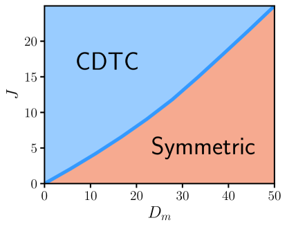
Figure 2: CDTC phase diagram in 2D based on the microscopic coupling $J$ and the variance of the microscopic noise $D_{m}$. Parameters from Eq. 15 are compared with numerical results from [61]. $\omega_{1}=(1+0.664)\pi$, $\omega_{2}=(1-0.664)\pi$, and $g=\nu=T=1$.

For parameters $\nu<\nu_{c}$, the Hamiltonian $H$, which describes the dynamics of the doubled time steps $2nT$, exhibits SSB such that

$$\langle\phi_{i}^{A}(2nT)\rangle=\textrm{constant},$$ (17)

i.e. is independent (to an extent that will be discussed in the next section) of $n$ and $i$ for arbitrarily small values of the perturbation parameter $\epsilon$. This parameter, which ensures the validity of the continuum limit, sets the correlation length and time of the order parameter. The above order parameter describes conventional SSB of a $\phi\rightarrow-\phi$ Ising symmetry that our system possesses at any one time step.

However, the dynamics for small $\epsilon$, as described by Eq. 10, are approximately linear and describe a period-doubled system (Eq. 8). Therefore a non-zero value of this conventional order parameter leads to odd step amplitudes

$$\langle\phi_{i}^{A}((2n+1)T)\rangle\simeq-\langle\phi_{i}^{A}(2nT)\rangle.$$ (18)

Combining this equation with the previous one leads to the conclusion of a discrete time symmetry breaking

$$(-1)^{n}\langle\phi_{i}^{A}(nT)\rangle=\textrm{constant},$$ (19)

in addition to the Ising symmetry breaking. This is the CDTC state we are interested in. The stability and robustness of this state will be discussed in Sec. IV.

III.1 CDTC order in one and higher dimensions

Based on the arguments in the previous section, the phases for a finite but possibly small range of $\epsilon$ are described by the phases of the Landau-Ginzburg Hamiltonian Eq. 15. This predicts CDTC ordered phases for arrays of coupled parametric oscillators in dimensions two and higher. However, most of the theoretical and experimental studies in the DTC as well as CDTC phases have occurred in one dimension. This is because one dimensional systems have fewer degrees of freedom and are easier to access. Unfortunately, finite temperature systems in one dimension formally lack an equilibrium phase transition [62]. In the case of DTCs, the prospect of many-body localization obstructing equilibriation overcomes this limitation. The cellular automata models for the CDTC [46, 39] evade this theorem through the use of long range interactions.

In the model considered in this work (Eq. 1), long range coupling between the parametric amplifiers can generate a phase transition in 1D. Specifically, we consider adding a long-range potential term to the Hamiltonian in Eq. 1, written as

$$U_{\alpha}=-J\sum_{i\neq j}\frac{\phi_{i}\phi_{j}}{|i-j|^{\alpha}}$$ (20)

with an arbitrary range parameter $\alpha$.

It was shown by Dyson that the Ising chain shows ferromagnetic order for $1<\alpha<2$ [63]. Combining this result with our arguments from the last sub-section, we expect a CDTC ordered phase for effective temperatures $D$ below a critical value that depends on $\alpha$ [64] as long as $1<\alpha<2$. This is consistent with the result cellular automata result from Ref. [46] which shows a CDTC regime is possible for $1<\alpha\lesssim 2$.

In this context it is interesting to compare the above results of our analysis to the results on the Frenkel-Kontorova model [39] which shows numerical evidence for a one dimensional chain of oscillators with nearest neighbor coupling. Since this model has a $\sin(\phi_{i})$ force term with a relatively large amplitude, the numerical results are presented for a relatively large non-linearity. Therefore, it is difficult to compare directly with our results unless parameters are tuned in the model to reduce the amplitude of the period-doubled oscillations.

However, as we will argue in the next section, the general structure of Eq. 15 survives even at finite non-linearity with modifications such as higher order (e.g. $\phi^{6}$) terms entering the analysis [60]. Such terms may explain the first order nature of the onset of CDTC order. The more serious contradiction between our results and Ref. [39] is that our analysis cannot explain CDTC order in 1D with short range interaction. However, even in 1D, our work does allow for low temperatures where the domain-wall energy $E_{\mathrm{DW}}$ computed from Eq. 15 is much smaller than temperature $D\ll E_{\mathrm{DW}}$. In this case, the effective 1D Ising model will be effectively ordered for system lengths $L\ll e^{E_{\mathrm{DW}}/D}$ (in units of lattice spacing). Such a model may show pre-thermal CDTC order derived from the quasi-order of the low temperature 1D Ising model. It should be noted however, that since our result is perturbative in $\epsilon$, it is difficult to determine whether the results of Ref. [39] are prethermal as suggested by the Ising model analysis or CDTC similar to Gács and Toom [65, 51].

IV Generalization beyond perturbation theory based on Markov chains

The results of the previous section can be shown to be robust by considering the CDTC order in a more general Markovian framework. To develop this framework, we start by noting that the dynamics on the doubled time-step described by Eq. 10 for $n=1$ can be solved iteratively to all orders in $\epsilon$ to obtain a dynamical map

$$\psi_{k}(2(n+1)T)=Q_{k^{\prime}}^{(2T)}\big{[}\{\psi_{k}(2nT)\}\big{]}$$ (21)

where $Q_{k}$ is a random functional of the displacement and momenta configurations $\{\psi_{k}\}$. This equation describes a Markov process relating time steps $t=2nT$ to $t=2(n+1)T$ with a transition probability

$$L^{(2T)}\big{[}\{\psi^{\prime}_{k^{\prime}}\}|\{\psi_{k}\}\big{]}=\Big{\langle}\delta\left(\psi^{\prime}_{k^{\prime}}-Q_{k}^{\prime}\big{[}\{\psi_{k}\}\big{]}\right)\Big{\rangle}_{Q}$$ (22)

Assuming that $L^{(2T)}$ is nonzero, such a Markov chain for a formally finite system is ergodic and evolves states towards a stationary probability $P[\{\psi_{k}\}]$, which can be obtained by solving the equation

$$\int D\psi^{\prime}_{k^{\prime}}\,L^{(2T)}\big{[}\{\psi_{k}\}|\{\psi^{\prime}_{k^{\prime}}\}\big{]}P\big{[}\{\psi^{\prime}_{k^{\prime}}\}\big{]}=P\big{[}\{\psi_{k}\}\big{]}.$$ (23)

To understand SSB in the stationary distribution $P$, we consider the dynamics of an analog of total Ising magnetization at even times $M_{e}\equiv\phi_{k=0}^{A}=\sum_{i}\phi_{i}^{A}$, which we call the order parameter (OP). Specifically, we can use this order parameter to bias the probability distribution $P$ to ${P}_{\varpi}=Pe^{-\varpi M}$ with an infinitesimal bias $\varpi$. Roughly, we take $\varpi\sim\mathcal{N}^{-1/2}$, enforcing the order of limits used in Ref. [60]. SSB occurs formally when

$$\left\langle{M_{e}}\right\rangle=\int D\psi_{k}\phi^{A}_{k=0}P_{\varpi}[\{\psi_{k}\}]=\textrm{sign}(\varpi)\bar{M}\mathcal{N}$$ (24)

where $\mathcal{N}$ is the system size and $\bar{M}$ is the average magnetization per site. In the thermodynamic limit, applying an infinitesimal bias field $\varpi$ leads to a nonzero probability $P_{\varpi}$ only in configurations where the sign of the OP matches the sign of $\varpi$. Such a biased stationary distribution reveals that SSB can be obtained by breaking the Ising symmetry.

By varying the field $\varpi$ in time, we can also break time-translation symmetry. Microscopically, we achieve this by adding a symmetry breaking force to Eq. 10 at time steps $2nT$. Since the only purpose of the force is to break the Ising and $T$-periodic time-translation symmetries, we achieve the same goal by modifying the transition probability separately for even and odd time steps

$$L^{(T,e)}_{\varpi}\big{[}\{\psi_{k}\}|\{\psi^{\prime}_{k^{\prime}}\}\big{]}=L^{(T)}\big{[}\{\psi_{k}\}|\{\psi^{\prime}_{k^{\prime}}\}\big{]}e^{-\varpi M[\{\psi_{k}\}]}$$

$$L^{(T,o)}_{\varpi}\big{[}\{\psi_{k}\}|\{\psi^{\prime}_{k^{\prime}}\}\big{]}=L^{(T)}\big{[}\{\psi_{k}\}|\{\psi^{\prime}_{k^{\prime}}\}\big{]}e^{+\varpi M[\{\psi^{\prime}_{k}\}]}.$$ (25)

Combining the two formulae using the observation that $L^{(2T)}=L^{(T,e)}*L^{(T,o)}$ leads to modification of the total $2T$ periodic transition probability

$$L^{(2T)}_{\varpi}=L^{(2T)}e^{-\varpi(M[\{\psi_{k}\}]-M[\{\psi^{\prime}_{k}\}])},$$ (26)

for which $P_{\varpi}$ is a stationary solution. Note that the stationary probability description of SSB is equivalent to a Hamiltonian formulation using

$$H=-\textrm{log}\,P_{\varpi}.$$ (27)

In this case, the infinitesimal bias becomes a field coupling term $-\varpi M\sum_{n}\delta(t-2nT)$.

By abruptly reversing the bias field $\varpi$ at time $t=0$, we can observe the slow equilibriation dynamics of the SSB system. After initializing in the $M>0$ regime, the system relaxes to the $M<0$ state on a timescale characterized by the mixing time $t_{\mathrm{mix}}$, which can also be viewed as the timescale of ergodicity between the symmetry broken states. Generally, the mixing time is exponential in the system size ($\log t_{\mathrm{mix}}\sim\mathcal{N}$) [54, 55]. In the thermodynamic limit, we can therefore restrict ourselves to the premixing regime $t<t_{\mathrm{mix}}$. Period-doubling persists if the magnetization at odd times is negative, leading to the condition

$$\left\langle{M_{o}}\right\rangle<0$$ (28)

where

$$\langle M_{o}\rangle =\int D\psi^{\prime}_{k^{\prime}}D\psi_{k}\,\phi^{A}_{k=0}$$

$$\qquad\times L^{(T,o)}_{\varpi>0}\big{[}\{\psi_{k}\}|\{\psi^{\prime}_{k^{\prime}}\}\big{]}P_{\varpi<0}\big{[}\{\psi^{\prime}_{k^{\prime}}\}\big{]}.$$ (29)

Any satisfactory Markov chain then describes a CDTC on an autocorrelation time-scale shorter than $t_{\mathrm{mix}}$.

An analogous condition applies if we flip the initial bias field $\varpi\rightarrow-\varpi$ and switch even and odd time steps. This parallel does not alter the relative sign of the OP for a CDTC order; i.e.

$$\sum_{\textrm{sign}(\varpi)=\pm 1}\left\langle{M_{e}}\right\rangle_{\varpi}\left\langle{M_{o}}\right\rangle_{\varpi}<0.$$ (30)

For systems with SSB, the total probability is the sum of the sectors—$P\simeq P_{\varpi>0}+P_{\varpi<0}$—and the distribution of $M_{o}$ is peaked when $\psi_{k}$ is given by $P_{\varpi}$, meaning $M_{o}P_{\varpi}\sim\left\langle{M_{o}}\right\rangle_{\varpi}P_{\varpi}$. Using these relations, the above condition for CDTC order can be approximated by the correlation $\left\langle{M_{o}M_{e}}\right\rangle$ and the condition Eq. 28 for CDTC order can be rewritten as a condition on the anticorrelation of the OP between neighboring times:

$$\left\langle{M_{o}M_{e}}\right\rangle= \int D\psi^{\prime}_{k^{\prime}}D\psi_{k}\,\phi^{A}_{k=0}\phi^{{}^{\prime}A}_{k^{\prime}=0}$$

$$\qquad\times L^{(T)}[\{\psi_{k}\}|\{\psi^{\prime}_{k^{\prime}}\}]P[\{\psi_{k^{\prime}}\}].$$ (31)

Note that by considering correlations, the above equation becomes independent of the external bias field $\varpi$. The derivation shows that the combination of the two equations Eq. 24 and Eq. 31 are sufficient to determine a CDTC order for a Markov process.

IV.1 Application to parametric oscillators

Let us now discuss how the system of parametric oscillators in Sec. III satisfies our criteria for a CDTC order. It is well-known [60] that the Boltzmann distribution associated with the GL Hamiltonian in Eq. 15 can satisfy Eq. 24 for appropriate parameters of $\nu$ and the cut-off. Note that while Eq. 15 is derived as a series expansion in $\epsilon$, the stationary probability $P$ can be defined for any $\epsilon$ and the GL Hamiltonian is generalized to Eq. 27. The exact Hamiltonian defined by Eq. 27 in terms of the stationary distribution would be a series in $\epsilon$ and would continue to show a SSB phase over a non-zero range of $\epsilon$. Similarly, considering the evolution equation for the amplified mode $\phi_{k}^{A}$ based on Eq. 10 for $n=1$ and $\epsilon\sim 0$ and the fact that $M_{k}\psi_{k}^{A}=-|\lambda_{k}|\psi_{k}^{A}=-\psi_{k}^{A}$, we find that $\phi_{k=0}^{A}(T)=-\phi_{k=0}^{A}(0)$. This sign flip leads to the equation

$$\phi_{k=0}^{A}\phi^{{}^{\prime}A}_{k=0}L^{(T)}\big{[}\{\psi_{k}\}|\{\psi^{\prime}_{k}\}\big{]}=-\left(\phi_{k=0}^{A}\right)^{2}L^{(T)}\big{[}\{\psi_{k}\}|\{\psi^{\prime}_{k}\}\big{]}.$$ (32)

This shows that the parametric oscillator model from Sec. III satisfies the second condition in Eq. 31. Since this condition is an inequality that is satisfied at $\epsilon=0$, it will also be satisfied for a non-zero range of $\epsilon$. Therefore the parametric oscillator model satisfies the CDTC order conditions Eq. 24 and Eq. 31.

IV.2 Application to dissipative quantum experiments

Because low temperature is a requirement for the realization of the CDTC order at small $\epsilon$, we expect that experiments with CDTC order can only occur in low temperature systems, which are often quantum. However, as discussed earlier, closed quantum (or classical) systems may have difficulty avoiding heating on a long time scale [25, 18]. This problem can be avoided in the presence of dissipation, which in principle leads to a finite temperature. In fact, evidence for dissipative quantum time crystals have already been observed in recent experiments [28]. While these systems do not have classical noise of the type above, they are described by a density matrix with a time-evolution written in terms of a Lindblad Master equation [26]. The solution to such a master equation can be written in terms of a transition superoperator $L^{(2T)}$ that evolves the density matrix $P$ over even time-steps. This leads to an equation for the stationary density matrix which is analogous to Eq. 23 with the probability $P$ replaced by a density matrix and $L^{(2T)}$ being replaced by a superoperator. The classical field $\psi_{k}$ can now be thought of as the indices of the density matrix and the resulting stationary density matrix can be written as the Boltzmann distribution of a Hamiltonian in Eq. 16 with a finite temperature. The equilibrium properties and phases of a finite temperature quantum phase qualitatively resemble a classical system indicating that our conclusions in this section are expected to apply to quantum systems as well. Similarly, the second condition for CDTC order, i.e. Eq. 31, also generalizes to the case of density matrices. Therefore, despite technically concerning classical systems, we expect our arguments to apply to quantum systems as well.

V Conclusion

Starting with a coupled array of period-doubling parametric amplifiers, we have considered the possibility of stabilizing a CDTC state by introducing Markovian noise and nonlinearity. In the absence of nonlinearities, such an array can be decomposed into a family of decoupled parametric amplifiers in momentum space. Such an oscillator can show amplification in a period-doubling channel for appropriate parameters. Fine tuning the damping close to the maximum amplification can ensure that the drive only amplifies modes near $k\sim 0$ as seen in Fig. 1. We found that in the limit of weak nonlinearity and noise, the random dynamics can be described by a Langevin equation which is linear in time (Eq. 14), in which the period-doubled $k\sim 0$ amplified mode ultimately leads to a stationary probability distribution. We find that the stationary probabilities are given by a Boltzmann distribution associated with a Ginzburg-Landau Hamiltonian (Eq. 15). This Hamiltonian is analogous to the GL theory of the Ising model which shows SSB (Eq. 17) in dimension two and higher or one. As discussed in Sec. III, for the limit of weak nonlinearity where the period-doubling parametric amplifier dominates the dynamics, such an order parameter breaks the discrete time-translation symmetry leading to a CDTC order. Similar observations find that long range interactions can lead to order in the corresponding one dimension equilibrium system. Prethermal order may appear in the short-ranged interacting one dimensional chains when the domain-wall energy is larger than temperature.

In  IV we explain how our results can be robust in a more general context of the conditions and properties of stationary states in Markov chain theory, which applies as long as the noise is uncorrelated. This relies on the SSB for the effective Hamiltonian (Eq. 27) derived from the stationary distribution of the doubled-time dynamics (Eq. 24). The discussion in this section only addresses the thermodynamic limit which is sufficient to understand the case of weakly anharmonic parametric amplifier. To determine the possibility of CDTC order, we then study the OP in the odd time-steps as well. We show that that a system which shows anti-correlation of the OP on neighboring time steps (see Eq. 31) together with SSB on even time steps is sufficient to show CDTC order. We check that these conditions are satisfied by the coupled parametric oscillator system for a non-zero range of $\epsilon$, which might be small. Furthermore, we expect this analysis to generalize to quantum systems as described in subsection  IV.2. A detailed verification of whether these results survive in the case of quantum systems would be an interesting future direction.

Since parametric amplifiers occur in many driven, weakly dissipative nonlinear systems such as Josephson junctions [66], nonlinear optics [67] and nonlinear electronic circuit elements [68], we are optimistic that this analysis can motivate experimental studies of CDTC symmetry breaking in more systems. In this context, we note that the analysis in this work only applies to systems with a microscopic damping $\Gamma$ that is of order unity, while the microscopic noise power scales as $\epsilon^{2}$. The fluctuation dissipation theorem then requires that the relevant systems must be low temperature open (i.e. strongly dissipative) systems. This restriction can in principle be relaxed by choosing the parameters to reduce the amplification of the parametric amplifier. However, this might limit the value of $\epsilon$ where the CDTC phase is realized. The low temperature condition may explain why quantum dissipative systems have been used so far to realize CDTC order [28]. Interesting future directions include details of the form of the symmetry breaking in the cases with stronger non-linearity (i.e. higher $\epsilon$) and whether dissipation generated by internal chaotic dynamics can also lead to a CDTC phase more generally.

Appendix A Details of parametric amplification

To achieve a $k=0$ period-doubled regime with amplified and squeezed modes, we explicitly write the trace of $\tilde{M}_{k=0}$ as

$$\tr\tilde{M}_{k=0}=2\cos\left(\theta_{1}+\theta_{2}\right)-\frac{\left(\theta_{1}-\theta_{2}\right)^{2}\sin\theta_{1}\sin\theta_{2}}{\theta_{1}\theta_{2}}$$

where $\theta_{i}=\Omega_{k=0,i}T/2$. Now we can set $\theta_{1}+\theta_{2}=\pi$ to make the first term $-2$. The trace then becomes

$$\tr\tilde{M}_{k=0}=-2-\frac{4\varphi^{2}\cos^{2}\varphi}{\frac{\pi^{2}}{4}-\varphi^{2}}$$

where $\varphi\equiv(\theta_{2}-\theta_{1})/2$. The minimum value of this trace, corresponding to the greatest amount of amplification, is the solution to a transcendental equation $\varphi-\frac{4}{\varphi}^{3}/\pi^{2}=\cot\varphi$ in the range $0<\varphi<\pi/2$. Numerically, this value is $0.332\pi$ which gives a minimum trace of $\approx-2.8$. We use this value throughout the paper.

Appendix B Explicit Formulae for Ginzburg-Landau Parameters

We give the explicit formulae for the parameters of the Ginzburg-Landau Hamiltonian in Eq. 15:

$$\zeta_{k,k_{1},k_{2}}= \int_{0}^{2T}d\tau\,A_{k}(2T-\tau)B_{k_{1}}(\tau)$$

$$\qquad\quad\times B_{k_{2}}(\tau)B_{k-k_{1}-k_{2}}(\tau)$$

$$\eta_{k}= \int_{0}^{2T}d\tau\,A_{k}(2T-\tau)W_{k}(\tau).$$ (33)

where

$$A_{k}(t) =\left[V_{k}^{-1}G_{k}(t)\right]_{12}$$

$$B_{k}(t) =\left[G_{k}(t)V_{k}\right]_{11}.$$

Here $V_{k}$ is the matrix with the eigenvectors of $G_{k}(T)$ as columns (amplified first).

After scaling $k\rightarrow k\sqrt{\epsilon}$ as described in Sec. III, the variance of $\eta_{k}$ becomes

$$2D =2D_{m}\int_{0}^{2T}d\tau\,\left(A_{0}(2t-\tau)\right)^{2}.$$ (34)

References

- Wilczek [2012] F. Wilczek, Physical Review Letters 109, 160401 (2012).
- Li et al. [2012] T. Li, Z.-X. Gong, Z.-Q. Yin, H. T. Quan, X. Yin, P. Zhang, L.-M. Duan, and X. Zhang, Physical Review Letters 109, 163001 (2012).
- Else et al. [2016] D. V. Else, B. Bauer, and C. Nayak, Physical Review Letters 117, 090402 (2016).
- Bruno [2013] P. Bruno, Physical Review Letters 111, 070402 (2013).
- Watanabe and Oshikawa [2015] H. Watanabe and M. Oshikawa, Physical Review Letters 114, 251603 (2015).
- Sacha [2015] K. Sacha, Physical Review A 91, 033617 (2015).
- Else et al. [2020] D. V. Else, C. Monroe, C. Nayak, and N. Y. Yao, Annual Review of Condensed Matter Physics 11, 467 (2020).
- Khemani et al. [2016] V. Khemani, A. Lazarides, R. Moessner, and S. Sondhi, Physical Review Letters 116, 250401 (2016).
- Moessner and Sondhi [2017] R. Moessner and S. L. Sondhi, Nature Physics 13, 424–428 (2017).
- Yao et al. [2017] N. Yao, A. Potter, I.-D. Potirniche, and A. Vishwanath, Physical Review Letters 118, 030401 (2017).
- Zhuang et al. [2021] Q. Zhuang, F. Machado, N. Y. Yao, and M. P. Zaletel, An absolutely stable open time crystal (2021), arXiv:2110.00585 [quant-ph] .
- D’Alessio and Rigol [2014] L. D’Alessio and M. Rigol, Physical Review X 4, 041048 (2014).
- Lazarides et al. [2014] A. Lazarides, A. Das, and R. Moessner, Physical Review E 90, 012110 (2014).
- Ponte et al. [2015a] P. Ponte, A. Chandran, Z. Papić, and D. A. Abanin, Annals of Physics 353, 196–204 (2015a).
- Lazarides et al. [2015] A. Lazarides, A. Das, and R. Moessner, Physical Review Letters 115, 030402 (2015).
- Ponte et al. [2015b] P. Ponte, Z. Papić, F. Huveneers, and D. A. Abanin, Physical Review Letters 114, 140401 (2015b).
- Lazarides and Moessner [2017] A. Lazarides and R. Moessner, Physical Review B 95, 195135 (2017).
- Hodson and Jarzynski [2021] W. Hodson and C. Jarzynski, Physical Review Research 3, 013219 (2021).
- Abanin et al. [2017] D. Abanin, W. De Roeck, W. W. Ho, and F. Huveneers, Communications in Mathematical Physics 354, 809–827 (2017).
- Else et al. [2017] D. V. Else, B. Bauer, and C. Nayak, Physical Review X 7, 011026 (2017).
- Zeng and Sheng [2017] T.-S. Zeng and D. N. Sheng, Physical Review B 96, 094202 (2017).
- Machado et al. [2020] F. Machado, D. V. Else, G. D. Kahanamoku-Meyer, C. Nayak, and N. Y. Yao, Physical Review X 10, 011043 (2020).
- Natsheh et al. [2021] M. Natsheh, A. Gambassi, and A. Mitra, Physical Review B 103, 224311 (2021).
- Keßler et al. [2020] H. Keßler, J. G. Cosme, C. Georges, L. Mathey, and A. Hemmerich, New Journal of Physics 22, 085002 (2020).
- Vu and Das Sarma [2023] D. Vu and S. Das Sarma, Physical Review Letters 130, 130401 (2023).
- Passarelli et al. [2022] G. Passarelli, P. Lucignano, R. Fazio, and A. Russomanno, Physical Review B 106, 224308 (2022).
- Lazarides et al. [2020] A. Lazarides, S. Roy, F. Piazza, and R. Moessner, Physical Review Research 2, 022002 (2020).
- Keßler et al. [2021] H. Keßler, P. Kongkhambut, C. Georges, L. Mathey, J. G. Cosme, and A. Hemmerich, Physical Review Letters 127, 043602 (2021).
- Choi et al. [2017] S. Choi, J. Choi, R. Landig, G. Kucsko, H. Zhou, J. Isoya, F. Jelezko, S. Onoda, H. Sumiya, V. Khemani, C. von Keyserlingk, N. Y. Yao, E. Demler, and M. D. Lukin, Nature 543, 221–225 (2017).
- Zhang et al. [2017] J. Zhang, P. W. Hess, A. Kyprianidis, P. Becker, A. Lee, J. Smith, G. Pagano, I.-D. Potirniche, A. C. Potter, A. Vishwanath, N. Y. Yao, and C. Monroe, Nature 543, 217–220 (2017).
- Pal et al. [2018] S. Pal, N. Nishad, T. Mahesh, and G. Sreejith, Physical Review Letters 120, 180602 (2018).
- Rovny et al. [2018] J. Rovny, R. L. Blum, and S. E. Barrett, Physical Review Letters 120, 180603 (2018).
- Ippoliti et al. [2021] M. Ippoliti, K. Kechedzhi, R. Moessner, S. Sondhi, and V. Khemani, PRX Quantum 2, 030346 (2021).
- Mi et al. [2021] X. Mi, M. Ippoliti, C. Quintana, A. Greene, Z. Chen, J. Gross, F. Arute, K. Arya, J. Atalaya, R. Babbush, J. C. Bardin, J. Basso, A. Bengtsson, A. Bilmes, A. Bourassa, et al., Nature 601, 531–536 (2021).
- Frey and Rachel [2022] P. Frey and S. Rachel, Science Advances 8, eabm7652 (2022).
- Kyprianidis et al. [2021] A. Kyprianidis, F. Machado, W. Morong, P. Becker, K. S. Collins, D. V. Else, L. Feng, P. W. Hess, C. Nayak, G. Pagano, N. Y. Yao, and C. Monroe, Science 372, 1192–1196 (2021).
- Beatrez et al. [2021] W. Beatrez, O. Janes, A. Akkiraju, A. Pillai, A. Oddo, P. Reshetikhin, E. Druga, M. McAllister, M. Elo, B. Gilbert, D. Suter, and A. Ajoy, Physical Review Letters 127, 170603 (2021).
- Beatrez et al. [2023] W. Beatrez, C. Fleckenstein, A. Pillai, E. de Leon Sanchez, A. Akkiraju, J. Diaz Alcala, S. Conti, P. Reshetikhin, E. Druga, M. Bukov, and A. Ajoy, Nature Physics 19, 407–413 (2023).
- Yao et al. [2020] N. Y. Yao, C. Nayak, L. Balents, and M. P. Zaletel, Nature Physics 16, 438–447 (2020).
- Van Der Pol and Van Der Mark [1927] B. Van Der Pol and J. Van Der Mark, Nature 120, 363–364 (1927).
- Strogatz [2018] S. H. Strogatz, Nonlinear dynamics and chaos with student solutions manual: With applications to physics, biology, chemistry, and engineering (CRC press, 2018).
- Hohenberg and Halperin [1977] P. C. Hohenberg and B. I. Halperin, Reviews of Modern Physics 49, 435 (1977).
- Brown et al. [1985] S. E. Brown, G. Mozurkewich, and G. Grüner, Solid state communications 54, 23 (1985).
- Yu et al. [1992] W. Yu, E. Harris, S. Hebboul, J. Garland, and D. Stroud, Physical Review B 45, 12624 (1992).
- Wiesenfeld and Satija [1987] K. Wiesenfeld and I. Satija, Physical Review B 36, 2483 (1987).
- Pizzi et al. [2021a] A. Pizzi, A. Nunnenkamp, and J. Knolle, Nature Communications 12, 1061 (2021a).
- Pizzi et al. [2021b] A. Pizzi, A. Nunnenkamp, and J. Knolle, Physical Review Letters 127, 140602 (2021b).
- Pizzi et al. [2021c] A. Pizzi, A. Nunnenkamp, and J. Knolle, Physical Review B 104, 094308 (2021c).
- Ye et al. [2021] B. Ye, F. Machado, and N. Y. Yao, Physical Review Letters 127, 140603 (2021).
- Citro et al. [2015] R. Citro, E. G. Dalla Torre, L. D’Alessio, A. Polkovnikov, M. Babadi, T. Oka, and E. Demler, Annals of Physics 360, 694–710 (2015).
- Toom [1974] A. L. Toom, Problemy Peredachi Informatsii 10, 70 (1974).
- Gács [2001] P. Gács, Journal of Statistical Physics 103, 45 (2001).
- Gray [2001] L. F. Gray, Journal of Statistical Physics 103, 1–44 (2001).
- Griffiths et al. [1966] R. B. Griffiths, C.-Y. Weng, and J. S. Langer, Physical Review 149, 301 (1966).
- Tomita and Miyashita [1992] H. Tomita and S. Miyashita, Physical Review B 46, 8886 (1992).
- Pizzi et al. [2020] A. Pizzi, D. Malz, G. De Tomasi, J. Knolle, and A. Nunnenkamp, Physical Review B 102, 214207 (2020).
- Landau and Lifshitz [1976] L. Landau and E. Lifshitz, Mechanics Third Edition: Volume 1 of Course of Theoretical Physics (Elsevier, 1976) Chap. 27.
- Floquet [1883] G. Floquet, Annales scientifiques de l’École Normale Supérieure 12, 47 (1883).
- Binder [1973] K. Binder, Physical Review B 8, 3423 (1973).
- Goldenfeld [2018] N. Goldenfeld, Lectures on phase transitions and the renormalization group (CRC Press, 2018).
- Schaich and Loinaz [2009] D. Schaich and W. Loinaz, Physical Review D 79, 056008 (2009).
- Ising [1925] E. Ising, Z. Phys 31, 253 (1925).
- Dyson [1969] F. J. Dyson, Communications in Mathematical Physics 12, 91–107 (1969).
- Nagle and Bonner [1970] J. Nagle and J. Bonner, Journal of Physics C: Solid State Physics 3, 352 (1970).
- Gács [1986] P. Gács, Journal of Computer and System Sciences 32, 15–78 (1986).
- Yaakobi et al. [2013] O. Yaakobi, L. Friedland, C. Macklin, and I. Siddiqi, Physical Review B 87, 144301 (2013).
- Galiffi et al. [2022] E. Galiffi, R. Tirole, S. Yin, H. Li, S. Vezzoli, P. A. Huidobro, M. G. Silveirinha, R. Sapienza, A. Alù, and J. Pendry, Advanced Photonics 4, 014002 (2022).
- Ranganathan and Tsividis [2003] S. Ranganathan and Y. Tsividis, IEEE Journal of Solid-State Circuits 38, 2087 (2003).