A New Paradigm for Generative Adversarial Networks based on Randomized Decision Rules

Abstract

The Generative Adversarial Network (GAN) was recently introduced in the literature as a novel machine learning method for training generative models. It has many applications in statistics such as nonparametric clustering and nonparametric conditional independence tests. However, training the GAN is notoriously difficult due to the issue of mode collapse, which refers to the lack of diversity among generated data. In this paper, we identify the reasons why the GAN suffers from this issue, and to address it, we propose a new formulation for the GAN based on randomized decision rules. In the new formulation, the discriminator converges to a fixed point while the generator converges to a distribution at the Nash equilibrium. We propose to train the GAN by an empirical Bayes-like method by treating the discriminator as a hyper-parameter of the posterior distribution of the generator. Specifically, we simulate generators from its posterior distribution conditioned on the discriminator using a stochastic gradient Markov chain Monte Carlo (MCMC) algorithm, and update the discriminator using stochastic gradient descent along with simulations of the generators. We establish convergence of the proposed method to the Nash equilibrium. Apart from image generation, we apply the proposed method to nonparametric clustering and nonparametric conditional independence tests. A portion of the numerical results is presented in the supplementary material.

Keywords: Minimax Game; Nonparametric Clustering; Nonparametric Conditional Independence Test; Stochastic Approximation; Stochastic Gradient MCMC

1 Introduction

The Generative Adversarial Network (GAN) (Goodfellow et al., 2014) provides a novel way for training generative models which seek to generate new data with the same statistics as the training data. Other than image generation, the GAN has been used in many nonparametric statistical tasks, such as clustering (Mukherjee et al., 2019), conditional independent test (Bellot and van der Schaar, 2019), and density estimation (Singh et al., 2018; Liu et al., 2021). In this paper, we call the training data real samples, and those generated by the GAN fake samples.

In its original design, the GAN is trained by competing two neural networks, namely generator and discriminator, in a game. However, due to the instability issues such as mode collapse (i.e., lack of diversity among fake samples), non-convergence, and vanishing or exploding gradients, the GAN is notoriously hard to train (Wiatrak and Albrecht, 2019). In this paper, we identify the reasons why the GAN suffers from the mode collapse issue: (i) The GAN evaluates fake samples at an individual level, lacking a mechanism for enhancing the diversity of fake samples; and (ii) the GAN tends to get trapped into a sub-optimal solution, lacking a mechanism for escaping from local traps (see Remark 1 for more explanations). To address this issue, we propose a new formulation for the GAN based on randomized decision rules. In this formulation, the similarity between the fake and real samples can be evaluated at the population level; and the generator is simulated from its posterior distribution conditioned on the discriminator using a stochastic gradient MCMC algorithm, thereby mitigating the difficulty of getting trapped in local optima.

Our contribution. The main contribution of this paper is three-fold: (i) we have provided a new formulation for the GAN based on statistical randomized decision theory, which allows the mode collapse issue to be fully addressed; (ii) we have proposed a training algorithm associated with the new formulation, and shown that its convergence to the Nash equilibrium is asymptotically guaranteed, or said differently, the proposed algorithm is immune to mode collapse as the number of iterations becomes large; (iii) we have developed a Kullback-Leibler divergence-based prior for the generator, which enhances the diversity of fake samples and further strengthens the effectiveness of the proposed method in overcoming the issue of mode collapse. The proposed method is tested on image generation, nonparametric clustering, and nonparametric conditional independence tests (in the supplementary material). Our numerical results suggest that the proposed method significantly outperforms the existing ones in overcoming the mode collapse issue.

Related Works. To tackle the mode collapse issue, a variety of methods have been proposed in the literature, see Wiatrak and Albrecht (2019) for a recent survey. These methods can be roughly grouped to two categories, namely, metric-based methods and mixture generator methods.

The methods in the first category strive to find a more stable and informative metric to guide the training process of the GAN. For example, Nowozin et al. (2016) suggested $f$-divergence, Mao et al. (2017) suggested $\chi^{2}$-divergence, Arjovsky et al. (2017) suggested Wasserstein distance, Binkowski et al. (2018) suggested maximum mean discrepancy, and Che et al. (2017) and Zhou et al. (2019) suggested some regularized objective functions. As mentioned previously, the GAN evaluates fake samples at the individual level and tends to get trapped to a sub-optimal solution. Therefore, the mode collapse issue is hard to resolve by employing a different metric unless (i) the objective function is modified such that the similarity between the fake and real samples can be enhanced at the population level, and (ii) a local-trap free optimization algorithm is employed for training. Recently, there has been a growing trend in the literature to incorporate gradient flow into the training of generative models, as explored by Gao et al. (2019). However, achieving this objective is generally considered a challenging task.

The methods in the second category are to learn a mixture of generators under a probabilistic framework with a similar motivation to this work. A non-exhaustive list of such types of methods include ensemble GAN (Wang et al., 2016), Mix+GAN (Arora et al., 2017), AdaGAN (Tolstikhin et al., 2017), MAD-GAN (Ghosh et al., 2018), MGAN (Hoang et al., 2018), Bayesian GAN (Saatci and Wilson, 2017), and ProbGAN (He et al., 2019). However, many of the methods are not defined in a proper probabilistic framework and, in consequence, the mode collapse issue cannot be overcome with a theoretical guarantee. In ensemble GAN, AdaGAN, MAD-GAN, Mix+GAN, and MGAN, only a finite mixture of generators is learned and thus the mode collapse issue cannot be overcome in theory. Bayesian GAN aims to overcome this obstacle by simulating the discriminator and generator from their respective conditional posterior distributions; however, the two conditional posterior distributions are incompatible and can lead unpredictable behavior (Arnold and Press, 1989). ProbGAN imposes an adaptive prior on the generator and updates the prior by successively multiplying the likelihood function at each iteration; consequently, the generator converges to a fixed point instead of a distribution.

The remaining part of this paper is organized as follows. Section 2 describes the new formulation for the GAN based on randomized decision rules. Section 3 proposes a training method and proves its convergence to the Nash equilibrium. Section 4 illustrates the performance of the proposed method using synthetic and real data examples. Section 5 concludes the paper with a brief discussion.

2 A New Formulation for GAN based on Randomized Decision Rules

2.1 Pure Strategy Minimax Game

In the original work Goodfellow et al. (2014), the GAN is trained by competing the discriminator and generator neural networks in a game. Let $\theta_{d}$ denote the parameters of the discriminator neural network, and let $D_{\theta_{d}}(x)$ denote its output function which gives a score for discriminating whether or not the input sample $x$ is generated from the data distribution $p_{data}$. Let $G_{\theta_{g}}(z)$ denote the generator neural network with parameter $\theta_{g}$, whose input $z$ follows a given distribution $q(z)$, e.g., uniform or Gaussian, and whose output distribution is denoted by $p_{\theta_{g}}$. Define

$$\begin{split}\mathcal{J}_{d}(\theta_{d};\theta_{g})&=\mathbb{E}_{x\sim p_{data}}\phi_{1}(D_{\theta_{d}}(x))+\mathbb{E}_{x\sim p_{\theta_{g}}}\phi_{2}(D_{\theta_{d}}(x)),\\ \mathcal{J}_{g}(\theta_{g};\theta_{d})&=-\mathbb{E}_{x\sim p_{data}}\phi_{1}(D_{\theta_{d}}(x))+\mathbb{E}_{x\sim p_{\theta_{g}}}\phi_{3}(D_{\theta_{d}}(x)),\end{split}$$ (1)

where $\phi_{1}(D)=\log(D)$, $\phi_{2}(D)=\log(1-D)$, and $\phi_{3}(D)=-\log(1-D)$ or $\log(D)$ are as defined in Goodfellow et al. (2014). The general form of the game introduced by Goodfellow et al. (2014) is given as follows:

$$\small(i)\ \ \max_{\theta_{d}}\mathcal{J}_{d}(\theta_{d};\theta_{g}),\quad(ii)\ \ \max_{\theta_{g}}\mathcal{J}_{g}(\theta_{g};\theta_{d}).$$ (2)

If $\phi_{3}=-\phi_{2}$, the objective of (2) represents a pure strategy minimax game, i.e.,

$$\small\min_{\theta_{g}}\max_{\theta_{d}}\mathcal{J}_{d}(\theta_{g},\theta_{d}),$$ (3)

which is called minimax GAN. If $\phi_{3}(D)=\log(D)$, the objective is said to be non-saturating, which results in the same fixed point of the dynamics as the minimax GAN but addresses the issue of vanishing gradient suffered by the latter. Quite recently, Zhou et al. (2019) proposed to penalize $\mathcal{J}_{d}(\theta_{d};\theta_{g})$ by a quadratic function of the Lipschitz constant of $\theta_{d}$, which addresses the gradient uninformativeness issue suffered by minimax GAN and improves its convergence.

2.2 Mixed Strategy Minimax Game

Let $\pi_{g}(\theta_{g})$ denote a distribution of generators. Based on the randomized decision theory, we define a mixed strategy minimax game:

$$\small\min_{\pi_{g}}\max_{\theta_{d}}\mathbb{E}_{\pi_{g}}\mathcal{J}_{d}(\theta_{d};\theta_{g}),$$ (4)

where $\mathcal{J}_{d}(\theta_{d};\theta_{g})$ is as defined in (1), and the expectation is taken with respect to $\pi_{g}(\theta_{g})$. That is, the game is to iteratively search for an optimal discriminator $\theta_{d}$ by maximizing $\mathbb{E}_{\pi_{g}}\mathcal{J}_{d}(\theta_{d};\theta_{g})$ for a given generator distribution $\pi_{g}$ and an optimal generator distribution $\pi_{g}$ by minimizing $\max_{\theta_{d}}\mathbb{E}_{\pi_{g}}\mathcal{J}_{d}(\theta_{d};\theta_{g})$ for a given discriminator $\theta_{d}$. In its Nash equilibrium, the discriminator is fixed and the generator is randomly drawn from the optimal generator distribution $\pi_{g}$, so the equilibrium is a mixed strategy Nash equilibrium. This is different from the pure strategy Nash equilibrium achieved by the minimax GAN, where both the discriminator and generator are fixed at equilibrium.

From the viewpoint of statistical decision theory, (4) is a minimax randomized decision problem, where $\pi_{g}$ can be viewed as a randomized decision rule and $\mathbb{E}_{\pi_{g}}\mathcal{J}_{d}(\theta_{d};\theta_{g})$ can be viewed as a risk function. Compared to the deterministic decision formulation (3), such a randomized decision formulation naturally accounts for the uncertainty of the generator and thus helps to address the mode collapse issue. Note that a deterministic decision rule is a special case of a randomized decision rule where one decision or action has probability 1. Further, Young and Smith (2005) (p.11) pointed out that a minimax randomized decision rule might perform better than all other deterministic decision rules under certain situations.

Let $p_{\pi_{g}}$ denote the distribution of the fake samples produced by the generators drawn from $\pi_{g}$, i.e., $p_{\pi_{g}}(x)=\int p_{\theta_{g}}(x)\pi_{g}(\theta_{g})d\theta_{g}$. Lemma 2.1 studies the basic property of the mixed strategy minimax game (4). The proof of this lemma, along with the proofs of other theoretical results in this paper, is provided in the supplement.

Lemma 2.1

Suppose the discriminator and generator have enough capacity, $\phi_{1}(D)=\log(D)$, and $\phi_{2}(D)=\log(1-D)$. For the game (4), $\min_{\pi_{g}}\max_{\theta_{d}}\mathbb{E}_{\pi_{g}}\mathcal{J}_{d}(\theta_{d};\theta_{g})=-\log(4)$. Further, if $\tilde{\theta}_{d}=\arg\max_{\theta_{d}}\mathbb{E}_{\tilde{\pi}_{g}}\mathcal{J}_{d}(\theta_{d};\theta_{g})$ for some $\tilde{\pi}_{g}$, then $(\tilde{\theta}_{d},\tilde{\pi}_{g})$ is a Nash equilibrium point if and only if $\mathbb{E}_{\tilde{\pi}_{g}}\mathcal{J}_{d}(\tilde{\theta}_{d};\theta_{g})$ $=-\log(4)$; at any Nash equilibrium point $(\tilde{\theta}_{d},\tilde{\pi}_{g})$, $p_{\tilde{\pi}_{g}}=p_{data}$ holds and $D_{\tilde{\theta}_{d}}(x)=1/2$ for any $x\sim p_{data}$, where $p_{\tilde{\pi}_{g}}=\int p_{\theta_{g}}\tilde{\pi}_{g}(\theta_{g})d\theta_{g}$ and $x\sim p_{data}$ means $x$ is distributed according to $p_{data}$.

Lemma 2.1 can be generalized to other choices of $\phi_{1}$ and $\phi_{2}$. In general, if $\phi_{1}$ and $\phi_{2}$ satisfy that (i) $\phi_{1}^{\prime}>0$, $\phi_{2}^{\prime}<0$, $\phi_{1}^{\prime\prime}\leq 0$, $\phi_{2}^{\prime\prime}\leq 0$, where $\phi_{i}^{\prime}$ and $\phi_{i}^{\prime\prime}$ denote the first and second derivatives of $\phi_{i}$ ($i=1,2$), respectively; and (ii) there exists some value $a$ such that $\phi_{1}^{\prime}(a)+\phi_{2}^{\prime}(a)=0$, then the conclusion of the lemma still holds except that $D_{\tilde{\theta}_{d}}\equiv a$ in this case.

2.3 Mixed Strategy Nash Equilibrium

Let $q_{g}(\theta_{g})$ denote the prior distribution of $\theta_{g}$, and let $N$ denote the training sample size. Define

$$\small\begin{split}\pi(\theta_{g}|\theta_{d},\mathcal{D})&\propto\exp\{\mathbb{J}_{g}(\theta_{g};\theta_{d})\}q_{g}(\theta_{g}),\end{split}$$ (5)

where

$$\small\mathbb{J}_{g}(\theta_{g};\theta_{d})=N\mathcal{J}_{g}(\theta_{g};\theta_{d})=N(-\mathbb{E}_{x\sim p_{data}}\phi_{1}(D_{\theta_{d}}(x))+\mathbb{E}_{x\sim p_{\theta_{g}}}\phi_{3}(D_{\theta_{d}}(x)),$$

and $\phi_{3}$ is an appropriately defined function, e.g., $\phi_{3}(D)=-\log(1-D)$ or $\log(D)$ as in Goodfellow et al. (2014). For the game (4), we propose to solve for $\theta_{d}$ by setting

$$\small\tilde{\theta}_{d}=\arg\max_{\theta_{d}}\int\mathcal{J}_{d}(\theta_{d};\theta_{g})\pi(\theta_{g}|\theta_{d},\mathcal{D})d\theta_{g},$$ (6)

where $\mathcal{J}_{d}(\theta_{d};\theta_{g})$ is as defined in (1) and then, with a slight abuse of notation, setting

$$\small\tilde{\pi}_{g}=\pi(\theta_{g}|\tilde{\theta}_{d},\mathcal{D}).$$ (7)

Theorem 2.1 shows that $(\tilde{\theta}_{d},\tilde{\pi}_{g})$ defined in (6)-(7) is a Nash equilibrium point for the game (4) as $N\to\infty$.

Theorem 2.1

Suppose that the discriminator and generator have enough capacity, $\phi_{1}(D)=\log(D)$, $\phi_{2}(D)=\log(1-D)$, $\phi_{3}=-\log(1-D)$, and the following conditions hold: (i) $\dim(\theta_{g})$, the dimension of the generator, grows with $N$ at a rate of $O(N^{\zeta})$ for some $0\leq\zeta<1$; and (ii) the prior density function $q_{g}(\theta_{g})$ is upper bounded on the parameter space $\Theta_{g}$ of the generator. Then $(\tilde{\theta}_{d},\tilde{\pi}_{g})$ defined in (6)-(7) is a Nash equilibrium point for the game (4) as $N\to\infty$.

Condition (ii) can be satisfied by many prior distributions, e.g., the uninformative prior $q_{g}(\theta_{g})\propto 1$ and the Gaussian prior. In addition, we consider an extra type of prior, namely, KL-prior, in this paper. The KL-prior is given by

$$\small q_{g}(\theta_{g})\propto\exp\{-\lambda D_{KL}(p_{data}|p_{\theta_{g}})\},$$ (8)

where $\lambda$ is a pre-specified constant, and the KL-divergence $D_{KL}(p_{data}|p_{\theta_{g}})$ can be estimated by a $k$-nearest-neighbor density estimation method (Pérez-Cruz, 2008; Wang et al., 2009) based on the real and fake samples. The motivation of this prior is to introduce to the proposed method a mechanism for enhancing the similarity between $p_{\theta_{g}}$ and $p_{data}$ at the density level. For the Gaussian prior, we generally suggest to set $\theta_{g}\sim\mathcal{N}(0,\sigma_{N}^{2}I_{\dim(\theta_{g})})$, where $\sigma_{N}^{2}\geq 1/(2\pi)$ and increases with the training sample size $N$ in such a way that the prior approaches uniformity asymptotically as $N\to\infty$.

There are ways other than (5)-(7) to define $(\tilde{\theta}_{d},\tilde{\pi}_{g})$ and still have Theorem 2.1 be valid. For example, one can define $\pi(\theta_{g}|\theta_{d},\mathcal{D})\propto\exp\{\mathbb{J}_{g}(\theta_{g};\theta_{d})/\tau\}$ $q_{g}(\theta_{g})$ or $\pi(\theta_{g}|\theta_{d},\mathcal{D})\propto\exp\{\mathbb{J}_{g}(\theta_{g};\theta_{d})/\tau\}(q_{g}(\theta_{g}))^{1/\tau}$ for some temperature $\tau>0$. That is, instead of the exact conditional posterior $\pi(\theta_{g}|\tilde{\theta}_{d},\mathcal{D})$, one can sample from its tempered version. In the extreme case, one may employ the proposed method to find the Nash equilibrium point for the minimax GAN in a manner of simulated annealing (Kirkpatrick et al., 1983).

Corollary 2.2

The conclusion of Theorem 2.1 still holds if the function $\phi_{3}(D)=-\log(1-D)$ is replaced with $\phi_{3}(D)=\log(D)$.

To make a more general formulation for the game (4), we can include a penalty term in $\mathcal{J}_{d}(\theta_{d};\theta_{g})$ such that

$$\small\mathcal{J}_{d}(\theta_{d};\theta_{g})=\mathbb{E}_{x\sim p_{data}}\phi_{1}(D_{\theta_{d}}(x))+\mathbb{E}_{x\sim p_{\theta_{g}}}\phi_{2}(D_{\theta_{d}}(x))-\lambda l(D_{\theta_{d}}),$$ (9)

where $l(D_{\theta_{d}})\geq 0$ denotes an appropriate penalty function on the discriminator. For example, one can set $l(D_{\theta_{d}})=\|D_{\theta_{d}}\|_{Lip}^{\alpha}$ for some $\alpha>1$, where $\|D_{\theta_{d}}\|_{Lip}$ denotes the Lipschitz constant of the discriminator. As explained in Zhou et al. (2019), including this penalty term enables the minimax GAN to overcome the gradient uninformativeness issue and improve its convergence. As implied by the proof of Lemma 2.1, where the mixture generator proposed in the paper can be represented as a single super generator, the arguments in Zhou et al. (2019) still apply and thus $\|D_{\tilde{\theta}_{d}}\|_{Lip}=0$ holds at the optimal discriminator $\tilde{\theta}_{d}=\arg\max_{\theta_{d}}\mathbb{E}_{\theta_{g}\sim\pi_{g}}\mathcal{J}_{d}(\theta_{d};\theta_{g})$. This further implies that the extra penalty term $-\lambda\|D_{\theta_{d}}\|_{Lip}^{\alpha}$ does not affect the definition of $\pi(\theta_{g}|\tilde{\theta}_{d},\mathcal{D})$ and, therefore, Theorem 2.1 still holds with (9).

3 Training Algorithm and Its Convergence

This section proposes an algorithm for solving the integral optimization problem (6) and studies its convergence to the Nash equilibrium.

3.1 The Training Algorithm

A straightforward calculation shows that

$$\small\begin{split}\nabla_{\theta_{d}}\int\mathcal{J}_{d}(\theta_{d};\theta_{g})\pi(\theta_{g}|\theta_{d},\mathcal{D})d\theta_{g}&=\mathbb{E}_{\pi_{g|d}}(\nabla_{\theta_{d}}\mathcal{J}_{d}(\theta_{d};\theta_{g}))\\ &+\mbox{Cov}_{\pi_{g|d}}(\mathcal{J}_{d}(\theta_{d};\theta_{g}),\nabla_{\theta_{d}}\mathbb{J}_{g}(\theta_{g};\theta_{d})),\end{split}$$

where $\mathbb{E}_{\pi_{g|d}}(\cdot)$ and $\mbox{Cov}_{\pi_{g|d}}(\cdot)$ denote the mean and covariance operators with respect to $\pi(\theta_{g}|\theta_{d},\mathcal{D})$, respectively. By Lemma 2.1, at any Nash equilibrium point we have $p_{\tilde{\pi}_{g}}=p_{data}$ and $D_{\tilde{\theta}_{d}}=1/2$. Then, following the arguments given in the proof of Theorem 2.1, it is easy to show by Laplace approximation that at the Nash equilibrium point $\mbox{Cov}_{\pi_{g|d}}(\mathcal{J}_{d}(\tilde{\theta}_{d};\theta_{g}),\nabla_{\theta_{d}}\mathbb{J}_{g}(\theta_{g};\tilde{\theta}_{d}))\to 0$ as $N\to\infty$. Therefore, when $N$ is sufficiently large, the target equation $\nabla_{\theta_{d}}\int\mathcal{J}_{d}(\theta_{d};\theta_{g})\pi(\theta_{g}|\theta_{d},\mathcal{D})d\theta_{g}=0$ can be solved by solving the mean field equation

$$h(\theta_{d})=\int H(\theta_{d},\theta_{g})\pi(\theta_{g}|\theta_{d},\mathcal{D})=0,$$ (10)

using a stochastic approximation algorithm, where $H(\theta_{d},\theta_{g})$ denotes an unbiased estimator of $\nabla_{\theta_{d}}\mathcal{J}_{d}(\theta_{d};\theta_{g})$. The convergence of the solution to the Nash equilibrium can be assessed by examining the plots described in Section 4. By the standard theory of stochastic approximation MCMC, see e.g., Benveniste et al. (1990); Andrieu et al. (2005); Deng et al. (2019); Dong et al. (2023), equation (10) can be solved by iterating between the following two steps, where $\theta_{d}^{(t)}$ denotes the estimate of the discriminator obtained at iteration $t$, and $\theta_{g}^{(t)}$ denotes a generic sample of the generator simulated at iteration $t$:

• Simulate $\theta_{g}^{(t)}$ by a Markov transition kernel which leaves the conditional posterior $\pi(\theta_{g}|\theta_{d}^{(t-1)},\mathcal{D})$ $\propto\exp\{\mathbb{J}_{g}(\theta_{g};\theta_{d}^{(t-1)})\}q_{g}(\theta_{g})$ invariant.

• Update the estimate of $\theta_{d}$ by setting $\theta_{d}^{(t)}=\theta_{d}^{(t-1)}+w_{t}H(\theta_{d}^{(t-1)},\theta_{g}^{(t)})$, where $w_{t}$ denotes the step size used at iteration $t$.

Stochastic gradient MCMC algorithms, such as stochastic gradient Langevin dynamics (SGLD) (Welling and Teh, 2011), stochastic gradient Hamiltonian Monte Carlo (SGHMC) (Chen et al., 2014) and momentum stochastic gradient Langevin dynamics (MSGLD) (Kim et al., 2022), can be used in step (i). Under appropriate conditions, we will show in Section 3.2 that $|\theta_{d}^{(t)}-\tilde{\theta}_{d}|\stackrel{{\scriptstyle p}}{{\to}}0$ and $\theta_{g}^{(t)}\stackrel{{\scriptstyle d}}{{\to}}\pi(\theta_{g}|\tilde{\theta}_{d},\mathcal{D})$ as $t\to\infty$, where $\stackrel{{\scriptstyle p}}{{\to}}$ and $\stackrel{{\scriptstyle d}}{{\to}}$ denote convergences in probability and distribution, respectively. That is, the proposed algorithm converges to the Nash equilibrium of the mixed strategy minimax game (4).

The proposed algorithm can also be viewed as an empirical Bayes-like method (Morris, 1983). For the case $\phi_{3}=-\phi_{2}$, the posterior $\pi(\theta_{g}|\theta_{d},\mathcal{D})$ can be expressed as

$$\small\pi(\theta_{g}|\theta_{d},\mathcal{D})\propto\exp\Big{\{}-\sum_{i=1}^{N}\phi_{1}(D_{\theta_{d}}(x_{i}))-N*\mathbb{E}_{z\sim q}\phi_{2}(D_{\theta_{d}}(G_{\theta_{g}}(z)))\Big{\}}q_{g}(\theta_{g}),$$ (11)

where $\theta_{d}$ can be viewed as a hyperparameter of the posterior; and the proposed algorithm is to determine $\theta_{d}$ by solving the equation

$$\small\frac{1}{N}\sum_{i=1}^{N}\nabla_{\theta_{d}}\left[\phi_{1}(D_{\theta_{d}}(x_{i}))+\mathbb{E}_{\pi_{g}}\mathbb{E}_{z\sim q}\phi_{2}(D_{\theta_{d}}(G_{\theta_{g}}(z_{i})))\right]=0.$$ (12)

In terms of the computational procedure, solving (12) is equivalent to maximizing the expected log-marginal posterior of $\theta_{d}$, which can be derived from (11) by imposing on $\theta_{d}$ an improper prior $\pi(\theta_{d})\propto 1$. To distinguish the proposed computational procedure from Bayesian GAN (Saatci and Wilson, 2017), we call it an empirical Bayes-like GAN (or EBGAN in short).

Algorithm 1 summarizes the proposed algorithm as a solver for (6), where $k_{g}$ generators are simulated using MSGLD (Kim et al., 2022) at each iteration, and the gradients are estimated with a mini-batch data of size $n$ at each iteration. More precisely, we have

$$\small\begin{split}\nabla_{\theta_{g}}\tilde{L}(\theta_{g},\theta_{d})&=\frac{N}{n}\sum_{i=1}^{n}\nabla_{\theta_{g}}\phi_{3}(D_{\theta_{d}}(G_{\theta_{g}}(z_{i})))+\nabla_{\theta_{g}}\log q_{g}(\theta_{g}),\\ H(\theta_{d},\theta_{g}^{(t)})&=\frac{1}{nk_{g}}\sum_{j=1}^{k_{g}}\sum_{i=1}^{n}\nabla_{\theta_{d}}\left[\phi_{1}(D_{\theta_{d}}(x_{i}^{*}))+\phi_{2}(D_{\theta_{d}}(G_{\theta_{g}^{j,(t)}}(z_{i})))\right],\\ \end{split}$$ (13)

where $\{x_{i}^{*}\}_{i=1}^{n}$ denotes a set of mini-batch data and $\{z_{i}\}_{i=1}^{n}$ denotes independent inputs for the generator. As illustrated by Kim et al. (2022), MSGLD tends to converge faster than SGLD, where the momentum bias term can help the sampler to escape from saddle points and accelerate its convergence in simulations on the energy landscape with pathological curvatures.

Algorithm 1 Empirical Bayesian GAN

  Input: Full data set $\mathcal{D}=\{x_{i}\}_{i=1}^{N}$, number of generators $k_{g}$, mini-batch size $n$, momentum smoothing factor $\alpha$, momentum biasing factor sequence $\{\rho_{t}\}_{t=1}^{\infty}$, learning rate sequence $\{\epsilon_{t}\}_{t=1}^{\infty}$, and step size sequence $\{w_{t}\}_{t=1}^{\infty}$.

  Initialization: $\theta_{0}$ from an appropriate distribution, set $m_{0}=0$;

  for $t=1,2,\dots,$ do

     (i) Sampling step:

     for $j=1,2,\dots,k_{g}$ do

        Draw a mini-batch data $\{x_{i}^{*}\}_{i=1}^{n}$, and set

        $\theta_{g}^{j,(t)}=\theta_{g}^{j,(t-1)}+\epsilon_{t}\left\{\nabla_{\theta_{g}}\tilde{L}(\theta_{g}^{j,(t-1)},\theta_{d}^{(t-1)})+\rho_{t-1}m^{j,(t-1)}\right\}+\mathcal{N}(0,2\tau\epsilon_{t})$,

        $m^{j,(t)}=\alpha m^{j,(t-1)}+(1-\alpha)\nabla_{\theta_{g}}\tilde{L}(\theta_{g}^{j,(t-1)},\theta_{d}^{(t-1)})$.

     end for

     (ii) Parameter estimating step: $\theta_{d}^{(t)}=\theta_{d}^{(t-1)}+w_{t}H(\theta_{d}^{(t-1)},\theta_{g}^{(t)})$, where $\theta_{g}^{(t)}=$ $(\theta_{g}^{1,(t)},\ldots,\theta_{g}^{k_{g},(t)})$.

  end for

Regarding hyperparameter settings, we have the following suggestions. In general, we set $w_{t}=c_{1}(t+c_{2})^{-\zeta_{1}}$ for some constants $c_{1}>0$, $c_{2}\geq 0$ and $\zeta_{1}\in(0,1]$, which satisfies Assumption 1. In this paper, we set $\zeta_{1}=0.75$ in all computations. Both the learning rate sequence and the momentum biasing factor sequence are required to converge to 0 as $t\to\infty$, i.e., $\lim_{t\to\infty}\epsilon_{t}=0$ and $\lim_{t\to\infty}\rho_{t}=0$. For example, one might set $\epsilon_{t}=O(1/t^{\zeta_{2}})$ and $\rho_{t}=O(1/t^{\zeta_{3}})$ for some $\zeta_{2},\zeta_{3}\in(0,1)$. In the extreme case, one might set them to small constants for certain problems, however, under this setting, the convergence of $\theta_{g}^{(t)}$ to the target posterior distribution will hold approximately even when $t\to\infty$. In this paper, we set $k_{g}=10$ and the momentum smoothing factor $\alpha=0.9$ as the default.

3.2 Convergence Analysis

Lemma 3.1 establishes the convergence of the discriminator estimator, and Lemma 3.2 shows how to construct the mixture generator desired for generating fake samples mimicking the real ones. For simplicity, we present the lemmas under the setting $k_{g}=1$.

Lemma 3.1 (Convergence of discriminator)

Suppose Assumptions 1-6 (given in the supplement) hold. If the learning rate $\epsilon_{t}$ is sufficiently small, then there exist a constant $\gamma$, an iteration number $t_{0}$ and an optimum $\tilde{\theta}_{d}=\arg\max_{\theta_{d}}$ $\int\mathcal{J}_{d}(\theta_{d};\theta_{g})\pi(\theta_{g}|\theta_{d},\mathcal{D})d\theta_{g}$ such that for any $t\geq t_{0}$,

$$\small\mathbb{E}\|\theta_{d}^{(t)}-\tilde{\theta}_{d}\|^{2}\leq\gamma w_{t},$$

where $t$ indexes iterations, $w_{t}$ is the step size satisfying Assumption 1, and an explicit formula of $\gamma$ is given in (S1.20).

As shown in (S1.20), the expression of $\gamma$ consists of two terms. The first term $\gamma_{0}$ depends only on the sequence $\{\omega_{t}\}$ and the stability constant of the mean field function $h(\theta_{d})$, while the second term characterizes the effects of the learning rate sequence $\{\epsilon_{t}\}$ and other constants (given in the assumptions) on the convergence of $\{\theta_{d}^{(t)}\}$. In particular, $\{\epsilon_{t}\}$ affects the convergence of $\{\theta_{d}^{(t)}\}$ via the upper bound of $\mathbb{E}\|\theta_{g}^{(t)}\|^{2}$. See Lemma S1 for the definition of the upper bound.

Lemma 3.2 (Ergodicity of generator)

Suppose Assumptions 1-7 (given in the supplement) hold. For a smooth test function $\psi(\theta_{g})$ with $\|\psi(\theta_{g})\|\leq C(1+\|\theta_{g}\|)$ for some constant $C$, define

$$\small\hat{\psi}_{T}=\frac{\sum_{t=1}^{T}\epsilon_{t}\psi(\theta_{g}^{(t)})}{\sum_{t=1}^{T}\epsilon_{t}},$$ (14)

where $T$ is the total number of iterations. Let $\bar{\psi}=\int\psi(\theta_{g})\pi(\theta_{g}|\tilde{\theta}_{d},\mathcal{D})d\theta_{g}$, $S_{T}=\sum_{t=1}^{T}\epsilon_{t}$, and $\Delta V_{t}=\nabla_{\theta_{g}}\tilde{L}(\theta_{g}^{(t)},\theta_{d}^{(t)})-\nabla_{\theta_{g}}L(\theta_{g}^{(t)},\theta_{d}^{(t)})$.

• Suppose the following conditions are satisfied: the momentum biasing factor sequence $\{\rho_{t}:\ t=1,2,\ldots\}$ decays to 0, the learning rate sequence $\{\epsilon_{t}:\ t=1,2,\ldots\}$ decays to 0, $\sum_{t=1}^{\infty}\epsilon_{t}=\infty$, and $\lim_{T\to\infty}\frac{\sum_{t=1}^{T}\epsilon_{t}^{2}}{\sum_{t=1}^{T}\epsilon_{t}}=0$. Then there exists a constant $C$ such that

  $$\small\mathbb{E}\|\hat{\psi}_{T}-\bar{\psi}_{T}\|^{2}\leq C\left(\sum_{t=1}^{T}\frac{\epsilon_{t}^{2}}{S_{T}^{2}}\mathbb{E}\|\Delta V_{t}\|^{2}+\frac{1}{S_{T}}+\frac{(\sum_{t=1}^{T}\epsilon_{t}^{2})^{2}}{S_{T}^{2}}\right).$$

• Suppose a constant learning rate of $\epsilon$ and a constant momentum biasing factor of $\rho$ are used. Then there exists a constant $C$ such that

  $$\small\mathbb{E}\|\hat{\psi}_{T}-\bar{\psi}\|^{2}\leq C\left(\frac{\sum_{t=1}^{T}\mathbb{E}\|\Delta V_{t}\|^{2}}{T^{2}}+\frac{1}{T\epsilon}+\epsilon^{2}+\rho^{2}\right).$$

The estimator (14) provides us a convenient way to construct $p_{\tilde{\pi}_{g}}$; that is, as $T\to\infty$, the corresponding mixture generator can contain all the generators simulated by Algorithm 1 in a run. We note that, by Theorem 1 of Song et al. (2020), the estimator (14) can be simplified to the simple path average $\hat{\psi}_{T}^{\prime}=\frac{1}{T}\sum_{t=1}^{T}\psi(\theta_{g}^{(t)})$ provided that $\epsilon_{t}\prec\frac{1}{t}$ holds, where $a_{t}\prec b_{t}$ means $\frac{a_{t}}{b_{t}}\to 0$ as $t\to\infty$. In practice, we can use only the generators simulated after the algorithm has converged or those simulated at the last iteration. For the latter, we may require $k_{g}$ to be reasonably large.

Remark 1

While the mixture generator produced by Algorithm 1 can overcome the mode collapse issue, a single generator might not, especially when an uninformative or Gaussian prior is used. Suppose that the uninformative prior $q_{g}(\theta_{g})\propto 1$ is used, $\phi_{3}(D)=-\log(1-D)$, and a discriminator $\tilde{\theta}_{d}$ with $D_{\tilde{\theta}_{d}}(x)=1/2$ for $x\in p_{data}$ has been obtained. With such a discriminator, there are many $\vartheta_{g}$’s maximizing $\mathbb{J}_{g}(\vartheta_{g};\tilde{\theta}_{d})$ as long as $p_{\vartheta_{g}}\subset p_{data}$, because the GAN evaluates the fake samples at the individual level. Here we use the notation $p_{\vartheta_{g}}\subset p_{data}$ to denote that the fake samples generated from $p_{\vartheta_{g}}$ resemble only a subset of the real samples. At such a point $(\tilde{\theta}_{d},\vartheta_{g})$, we have $\mathcal{J}_{d}(\tilde{\theta}_{d};\vartheta_{g})=-\log 4$ and $-\mathbb{J}_{g}(\vartheta_{g};\tilde{\theta}_{d})=-N\log 4$. The latter means that the generator has attained its minimum energy, although $p_{\vartheta_{g}}\subset p_{data}$ is still sub-optimal; in other words, such a generator is trapped to a sub-optimal solution. However, if Algorithm 1 is run for sufficiently long time and the generators from different iterations are used for estimation, we can still have $\frac{1}{Tk_{g}}\sum_{t=1}^{T}\sum_{i=1}^{k_{g}}\int p_{\vartheta_{g,i}^{(t)}}\pi(\vartheta_{g,i}^{(t)}|\tilde{\theta}_{d}^{(t)},\mathcal{D})d\vartheta_{g,i}^{(t)}\approx p_{data}$ by assembling many sub-optimal generators (provided the learning rate $\epsilon_{t}\prec 1/t$), where $\vartheta_{g,i}^{(t)}$ denotes the $i$th generator at iteration $t$ and $\tilde{\theta}_{d}^{(t)}$ denotes the discriminator at iteration $t$. That is, using mixture generator is a valid way for overcoming the mode collapse issue. For the case of $\phi_{3}(D)=\log(D)$ and the case of the Gaussian prior, this is similar. The KL-prior provides a stronger force to drive $\frac{1}{k_{g}}\sum_{i=1}^{k_{g}}\int p_{\vartheta_{g,i}^{(t)}}\pi(\vartheta_{g,i}^{(t)}|\tilde{\theta}_{d}^{(t)},\mathcal{D})d\vartheta_{g,i}^{(t)}$ to $p_{data}$ as $t\to\infty$, while the choice of $k_{g}$ is not crucial.

4 Numerical Studies

We illustrate the performance of the EBGAN using various examples. Due to the space limit, some of the examples are presented in the supplement.

4.1 A Gaussian Example

Consider a 2-D Gaussian example, where the real samples are generated in the following procedure (Saatci and Wilson, 2017): (i) generate the cluster mean: $\mu\sim\mathcal{N}(0,I_{2})$, where $I_{2}$ denotes a 2-dimensional identity matrix; (ii) generate a mapping matrix $M\in\mathbb{R}^{2\times 2}$ with each element independently drawn from $\mathcal{N}(0,1)$; (iii) generate 10,000 observations: $x_{i}\sim(\mathcal{N}(0,I_{2})+\mu)\times M^{T}$, for $i=1,2,\ldots,10,000$. The code used for data generation is available at https://github.com/andrewgordonwilson/bayesgan/blob/master/bgan_util.py. Both the discriminator and generators used for this example are fully connected neural networks with ReLU activation. The discriminator has a structure of $2-1000-1$, and the generator has a structure of $10-1000-2$.

The original GAN (Goodfellow et al., 2014) was first applied to this example with the parameter settings given in the supplement. Figure 1(a) shows the empirical means of $D_{\theta_{d}^{(t)}}(x)$ and $D_{\theta_{d}^{(t)}}(\tilde{x})$ along with iterations, where $x$ represents a real sample and $\tilde{x}$ represents a fake sample simulated by the generator. For the given choices of $\phi_{1}$ and $\phi_{2}$, as implied by Lemma 2.1, we should have $\mathbb{E}(D_{\theta_{d}^{(t)}}(x))=\mathbb{E}(D_{\theta_{d}^{(t)}}(\tilde{x}))=0.5$ at the Nash equilibrium. As shown by Figure 1(a), the GAN did reach the 0.5-0.5 convergence. However, as shown by Figure 1(b), the generator still suffers from the mode collapse issue at this solution, where the fake samples resemble only a subset of the real samples. As mentioned previously, this is due to the reasons: The GAN evaluates the fake samples at the individual level, lacking a mechanism for enhancing the diversity of fake samples, and tends to get trapped at a sub-optimal solution for which $p_{\theta_{g}}\subset p_{data}$ holds while the ideal objective value $-\log 4$ can still be attained.

The mode collapse issue can be tackled by EBGAN, for which we consider both the KL-prior and Gaussian prior.

4.1.1 KL-prior

The KL-prior is given in (8), which enhances the similarity between $p_{\theta_{g}}$ and $p_{data}$ at the density level. For this example, we set $\lambda=100$, set $k=1$ for $k$-nearest-neighbor density estimation (see Pérez-Cruz (2008) for the estimator), and used the auto-differentiation method to evaluate the gradient $\nabla_{\theta_{g}}\log q_{g}(\theta_{g})$. Figure 1(c)&(d) summarize the results of EBGAN for this example with $\phi_{3}(D)=\log(D)$ and $k_{g}=10$. The settings for the other parameters can be found in the supplement. For EBGAN, Figure 1(c) shows that it converges to the Nash equilibrium very fast, and Figure 1(d) shows that the fake samples simulated by a single generator match the real samples almost perfectly.

In summary, this example shows that EBGAN can overcome the mode collapse issue by employing a KL-prior that enhances the similarity between $p_{\theta_{g}}$ and $p_{data}$ at the density level.

(a)	(b)
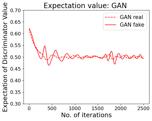
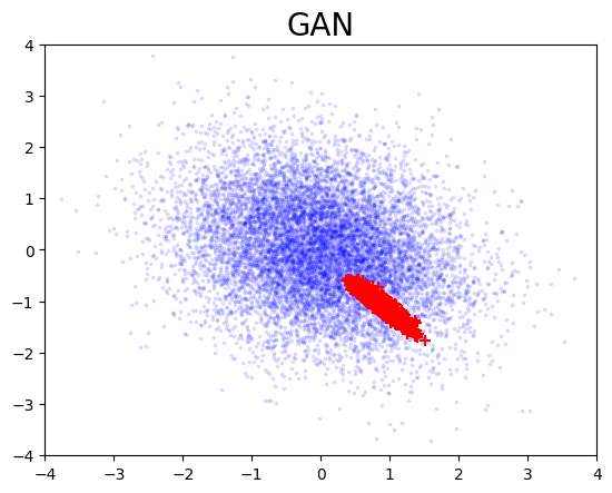
(c)	(d)

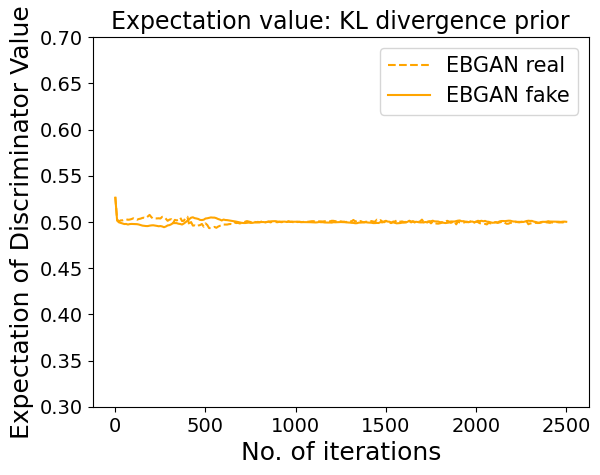
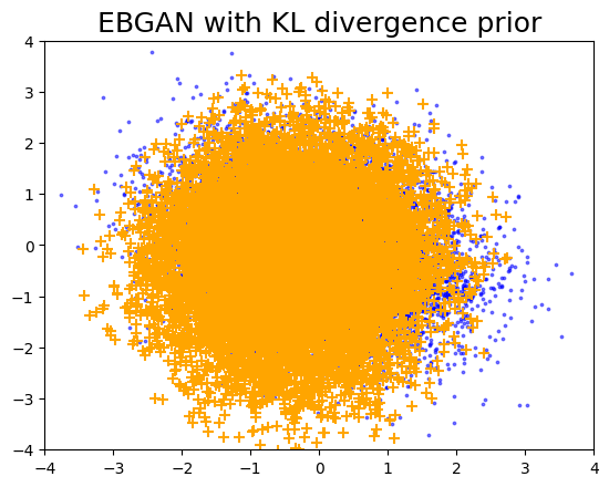
Figure 1: Illustration of the mode collapse issue: (a) empirical means of $D_{\theta_{d}^{(t)}}(x_{i})$ and $D_{\theta_{d}^{(t)}}(\tilde{x}_{i})$ produced by GAN; (b) coverage plot of the real (dots) and fake samples (‘+’) generated by GAN; (c) empirical means of $D_{\theta_{d}^{(t)}}(x_{i})$ and $D_{\theta_{d}^{(t)}}(\tilde{x}_{i})$ produced by EBGAN; (d) coverage plot of the real (dots) and fake samples (‘+’) generated by a single generator of EBGAN.

4.1.2 Gaussian prior

We have also tried the simple Gaussian prior $\theta_{g}\sim N(0,I_{d})$ for this example. Compared to the KL-divergence prior, the Gaussian prior lacks the ability to enhance the similarity between $p_{\theta_{g}}$ and $p_{data}$, but it is much cheaper in computation. For this example, we have run EBGAN with $\phi_{3}(D)=\log(D)$ and $k_{g}=10$. The settings for other parameters can be found in the supplement. To examine the performance of EBGAN with this cheap prior, we made a long run of 30,000 iterations. For comparison, the GAN was also applied to this example with $\phi_{3}(D)=\log(D)$. Figure S1 (in the supplement) shows the empirical means of $D_{\theta_{d}^{(t)}}(x)$ and $D_{\theta_{d}^{(t)}}(\tilde{x})$ produced by the two methods along with iterations, which indicates that both methods can reach the 0.5-0.5 convergence very fast. Figure 2 shows the evolution of the coverage plot of fake samples. Figure 2(a) indicates that the GAN has not reached the Nash equilibrium even with 25,000 iterations. In contrast, Figure 2(b) shows that even with the cheap Gaussian prior, the EBGAN can approximately reach the Nash equilibrium with 25,000 iterations, although it also suffers from the mode collapse issue in the early stage of the run. Figure 2(c) shows that for the EBGAN, the mode collapse issue can be easily overcome by integrating multiple generators.

(a) Evolution of coverage by GAN

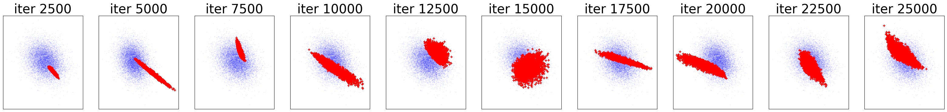
(b) Evolution of coverage by one generator from EBGAN

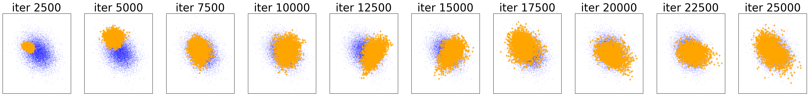
(c) Evolution of coverage by integration of 10 generators from EBGAN

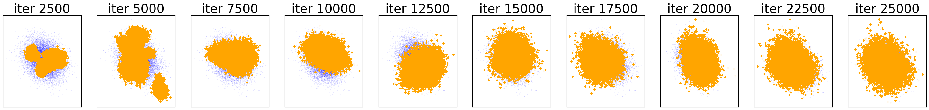
Figure 2: Coverage plots produced by (a) GAN, (b) a single generator of EBGAN, and (c) all 10 generators of EBGAN, where the generators for the plots from left to right are collected at iterations 2500, 5000, $\ldots$, 25000, respectively. The dot points (in blue) represent real samples; and ‘+’ points represent fake samples produced by GAN (in red) or EBGAN (in yellow).

Finally, we note that the convergence of the GAN and EBGAN should be checked in two types of plots, namely, empirical convergence plot of $\mathbb{E}D_{\theta_{d}^{(t)}}(x)$ and $\mathbb{E}D_{\theta_{d}^{(t)}}(\tilde{x})$, and coverage plot of the fake and real samples. The former measures how well an individual fake sample fits into the population of real samples, while the latter measures the diversity of fake samples, i.e., whether a wide range of fake samples is generated.

4.2 A Mixture Gaussian Example

To further illustrate the performance of the EBGAN, we consider a more complex example which was taken from Saatci and Wilson (2017). The dataset was generated from a 10-component mixture Gaussian distribution in the following procedure: (i) generate 10 cluster means: $\mu^{(j)}\sim\mathcal{N}(0,25I_{2})$, $j=1,2,\ldots,10$, where $I_{2}$ denotes a 2-dimensional identity matrix; (ii) generate 10 mapping matrices: $M^{(j)}\in\mathbb{R}^{100\times 2}$ for $j=1,2,\ldots,10$, with each element of the matrices independently drawn from $\mathcal{N}(0,25)$. (iii) generate 1000 observations of $x^{(j)}$ for each $(\mu^{(j)},M^{(j)})$: $x_{i}^{(j)}\sim(\mathcal{N}(0,I_{2})*0.5+\mu^{(j)})\times(M^{(j)})^{T}$, for $j=1,2,\ldots,10$, $i=1,2,\ldots,1000$.

For this example, the EBGAN was run with the prior $q_{g}=\mathcal{N}(0,I)$, $k_{g}=10$, and $\phi_{3}(D)=-\log(1-D)$ and $\log(D)$. The discriminator has a structure of $100-1000-1$ and the generator has a structure of $10-1000-100$, which are the same as those used in Saatci and Wilson (2017). The results with $\phi_{3}(D)=-\log(1-D)$ are presented below and those with $\phi_{3}(D)=\log(D)$ are presented in the supplement.

(a)	(b)	(c)
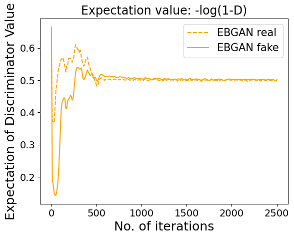
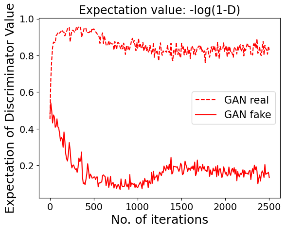
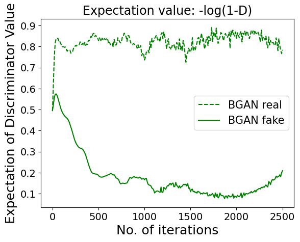
(d)	(e)	(f)

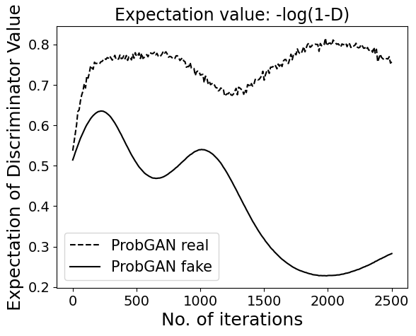
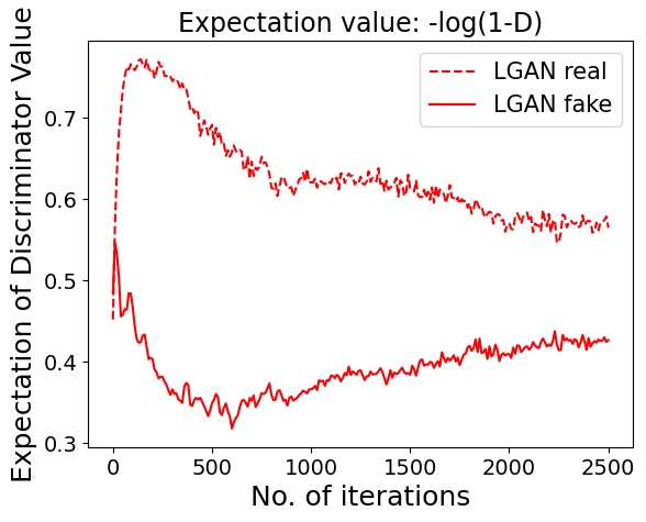
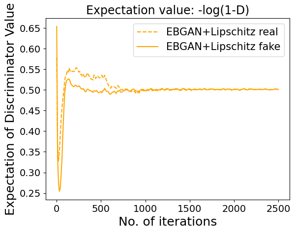
Figure 3: Nash equilibrium convergence plots with $\phi_{3}(D)=-\log(1-D)$, which compare the empirical means of $D_{\theta_{d}^{(t)}}(x_{i})$ and $D_{\theta_{d}^{(t)}}(\tilde{x}_{i})$ produced by different methods along with iterations: (a) EBGAN, (b) minimax GAN, (c) Bayesian GAN, (d) ProbGAN, (e) Lipschitz-GAN, (f) EBGAN with a Lipschitz penalty.

For comparison, the minimax GAN (Goodfellow et al., 2014), Bayesian GAN (Saatci and Wilson, 2017), ProbGAN (He et al., 2019), and Lipschitz GAN (Zhou et al., 2019) were applied to this example with the parameter settings given in the supplement. For all the four methods, we employed the same settings of $\phi_{1}$, $\phi_{2}$ and $\phi_{3}$ and the same discriminator and generator as the EBGAN. For a thorough comparison, we have tried to train the EBGAN with a Lipschitz penalty.

Figure 3 examines the convergence of $\mathbb{E}(D_{\theta_{d}^{(t)}}(x))$ and $\mathbb{E}(D_{\theta_{d}^{(t)}}(\tilde{x}))$. It indicates that except for the EBGAN, none of the four methods, minimax GAN, Bayesian GAN, ProbGAN and Lipschitz-GAN, has reached the 0.5-0.5 convergence. Compared to Figure 3(a), Figure 3(f) shows that the Lipschitz penalty improves the convergence of the EBGAN slightly.

Other than the convergence plots of $\mathbb{E}(D_{\theta_{d}^{(t)}}(x))$ and $\mathbb{E}(D_{\theta_{d}^{(t)}}(\tilde{x}))$, we checked whether the fake samples recover all 10 components of the mixture distribution, where the principal component analysis (PCA) was used for high-dimensional data visualization. For EBGAN, we used only the generators obtained at the last iteration: we simulated 1000 fake samples from each of $k_{g}=10$ generators. As shown in Figure 4, EBGAN recovered all 10 components in both cases with or without the penalty term, while the other four methods failed to do so. The minimax GAN and Lipschitz GAN, both of which work with a single generator, failed for this example. The BGAN and ProbGAN worked better than minimax GAN, but still missed a few components. In the supplement, we compared the performance of different methods with $\phi_{3}=\log(D)$. The results are very similar to Figure 3 and Figure 4.

For the EBGAN, we have also tried to use generators simulated at multiple iterations, e.g., those in the last 2000 iterations. We found that the component recovery plot can be further improved. For simplicity, we used only the generators obtained at the last iteration. If the EBGAN is run with a larger value of $k_{g}$, the overlapping area can also be further improved.

(a)	(b)	(c)
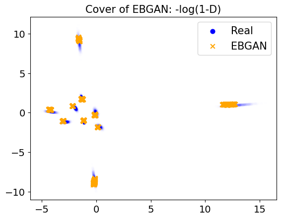
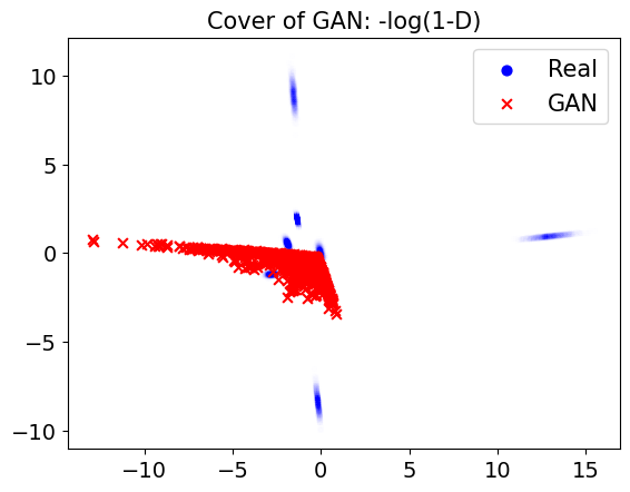
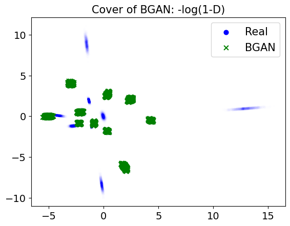
(d)	(e)	(f)

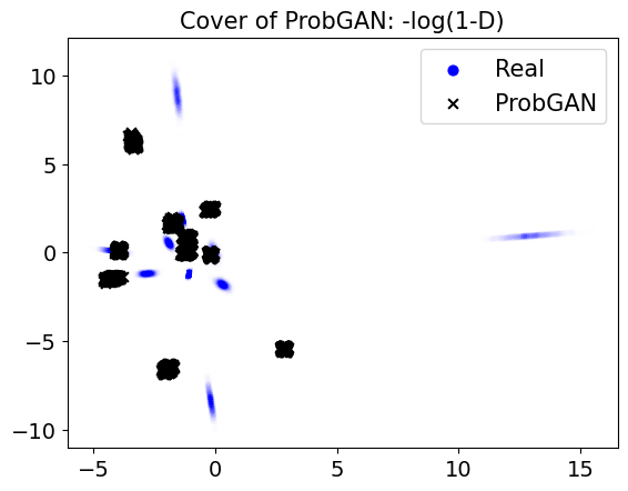
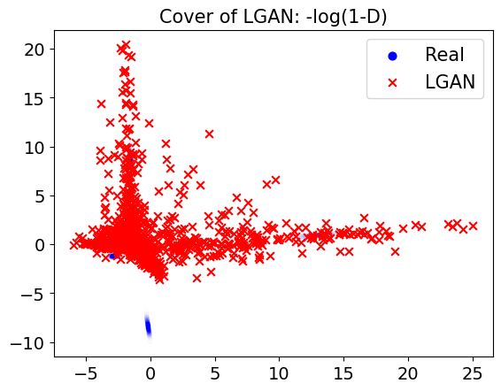
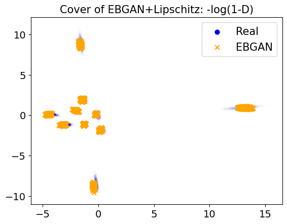
Figure 4: Component recovery plots with $\phi_{3}(D)=-\log(1-D)$: (a) EBGAN with $\lambda=0$, (b) minimax GAN, (c) BGAN, (d) ProbGAN, (e) Lipschitz GAN, and (f) EBGAN with a Lipschitz penalty.

In summary, EBGAN performs very well for this mixture example: the fake samples generated by it exhibit both good quality and diversity. The comparison with existing methods indicates that integrating multiple generators is essential for overcoming the mode collapse issue, particularly when the objective function lacks a mechanism to enhance the similarity between $p_{\theta_{g}}$ and $p_{data}$ at the density level.

4.3 Image Generation

Fashion-MNIST is a dataset of 60,000 training images and 10,000 test images. Each image is of size $28\times 28$ and has a label from 10 classes: T-shirt, Trouser, $\ldots$, Ankle boot. The full description for the dataset can be found at https://github.com/zalandoresearch/fashion-mnist.

For this example, we compared EBGAN with GAN, BGAN and ProbGAN with parameter settings given in the supplement. The results are summarized in Figure 5 and Table 1. Figure 5 shows that for this example, the EBGAN can approximately achieve the 0.5-0.5 convergence for $\mathbb{E}(D_{\theta_{d}^{(t)}}(x_{i}))$ and $\mathbb{E}(D_{\theta_{d}^{(t)}}(\tilde{x}_{i}))$; that is, the EBGAN can produce high quality images which are almost indistinguishable from real ones. However, none of the existing three methods can achieve such good convergence.

(a)	(b)	(c)	(d)	(e)

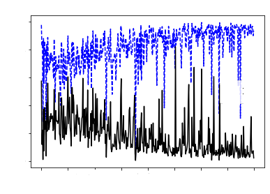
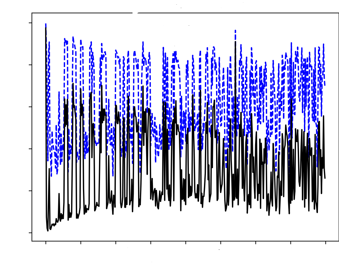
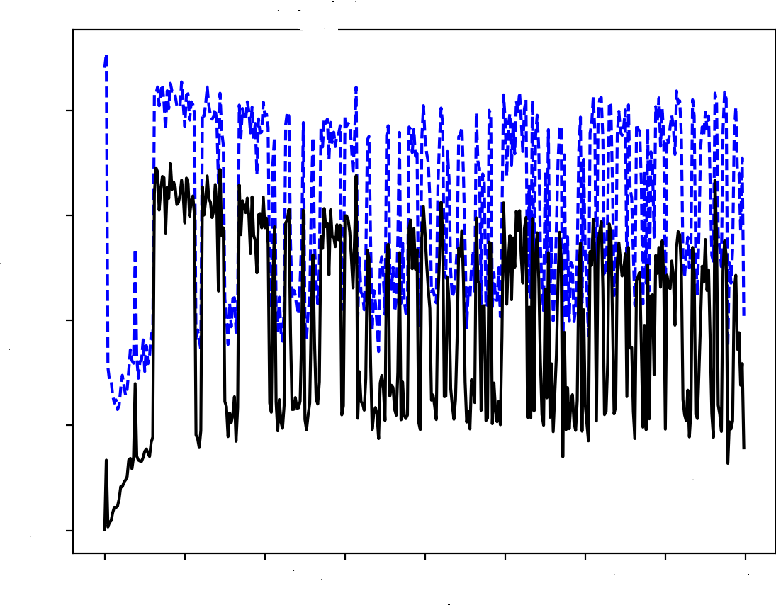
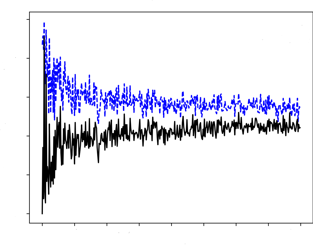
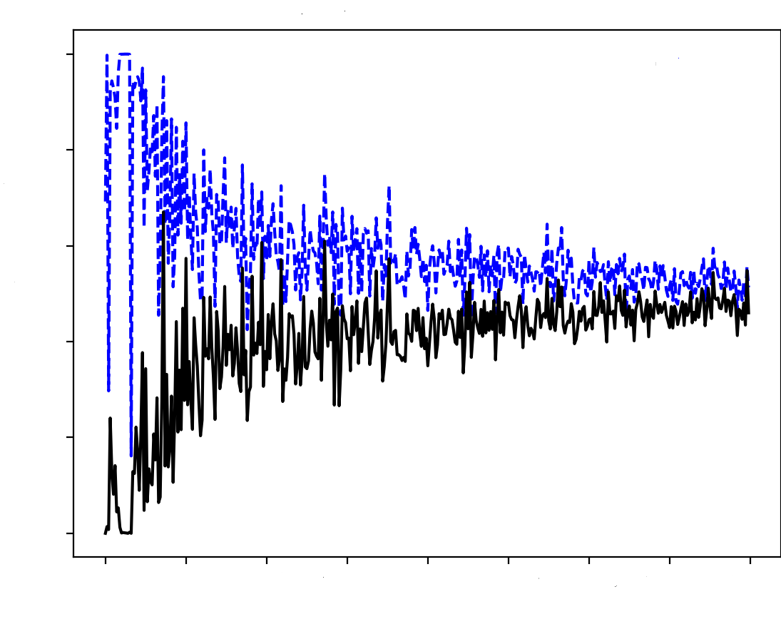
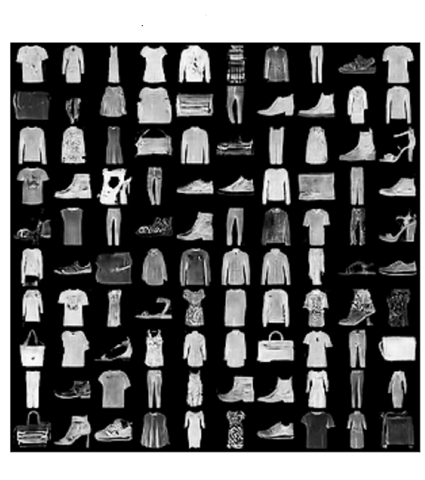
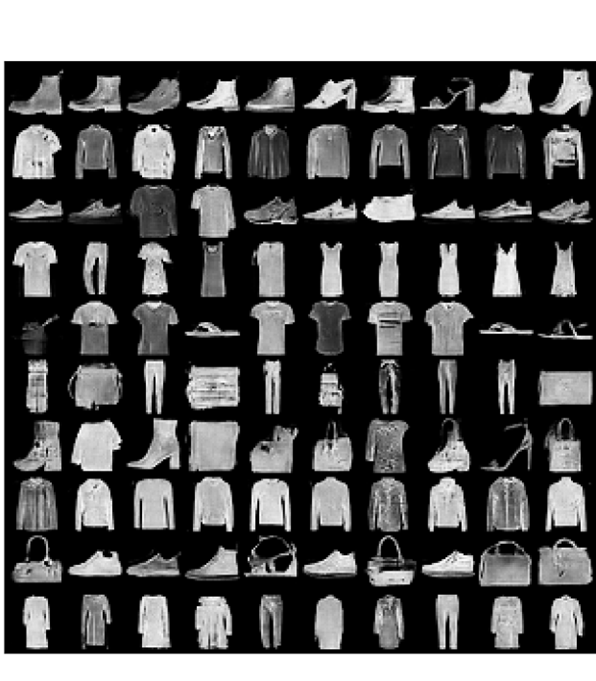
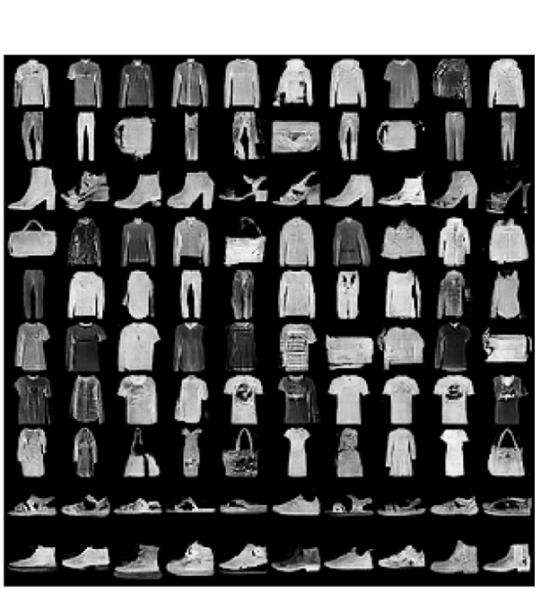
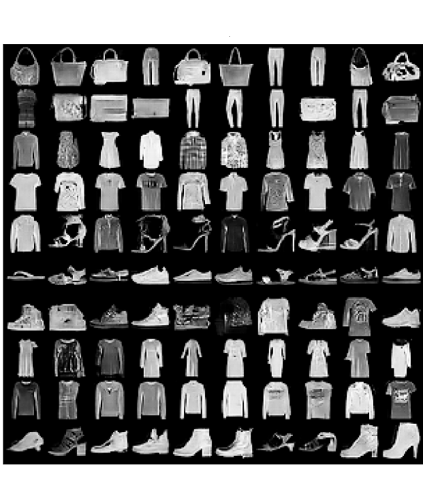
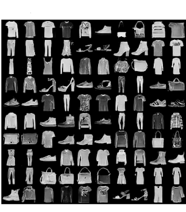
Figure 5: Convergence plots and images produced by (a) GAN, (b) Bayesian GAN, (c) ProbGAN, (d) EBGAN with a KL-divergence prior, and (e) EBGAN with a Gaussian prior. For each of the convergence plots, $x$-axis represents iterations, ranging from 0 to 40,000; and $y$-axis represents the empirical mean of discriminator values, ranging from 0 to 1.0, where dotted and solid lines are for real and fake samples, respectively.

Table 1: Average IS, 1-WD, and MMD values produced by different methods for Fashion MNIST, where the averages and standard deviations (given in the parentheses) were calculated based on 5 independent runs.

Method GAN Bayesian GAN ProbGAN EBGAN(KL) EBGAN(Gaussian) IS 7.525 (0.011) 7.450 (0.044) 7.384 (0.056) 7.606 (0.035) 7.712 (0.024) 1-WD 6.360 (0.012) 6.363 (0.015) 6.367 (0.024) 6.356 (0.015) 6.287 (0.025) MMD 0.276 (0.002) 0.277 (0.002) 0.276 (0.002) 0.257 (0.001) 0.275 (0.003)

We further assess the quality of images generated by different methods using three metrics: inception scores (IS) (Salimans et al., 2016), first moment Wasserstein distance (1-WD), and maximum mean discrepancy (MMD). Refer to Section S2 of the supplement for their definitions and calculation procedures. The results are summarized in Table 1, which indicates the superiority of the EBGAN in image generation.

4.4 Nonparametric Clustering

Clustering has been extensively studied in unsupervised learning with classical methods such as expectation-maximization (EM) (Dempster et al., 1977) and K-means. Although its main focus is to group data into different classes, it would be even more beneficial if clustering was done along with dimension reduction, as it enhances the interpretability of clusters. This simultaneous goal of clustering and dimension reduction can be achieved through generative clustering methods such as Cluster GAN (Mukherjee et al., 2019) and GAN-EM (Zhao et al., 2019).

Since the cluster structure is generally not retained in the latent space of the GAN, Cluster GAN modifies the structure of the GAN to include an encoder network, which enforces precise recovery of the latent vector so that it can be used for clustering. Let the encoder be parameterized by $\theta_{e}$. Cluster GAN works with the following two objective functions:

$$\small\begin{split}\mathcal{J}_{d}(\theta_{d};\theta_{g})&=\mathbb{E}_{x\sim p_{data}}\phi_{1}(D_{\theta_{d}}(x))+\mathbb{E}_{x\sim p_{\theta_{g}}}\phi_{2}(D_{\theta_{d}}(x)),\\ \mathcal{J}_{g,e}(\theta_{g},\theta_{e};\theta_{d})&=-\mathbb{E}_{x\sim p_{data}}\phi_{1}(D_{\theta_{d}}(x))+\mathbb{E}_{x\sim p_{\theta_{g}}}\phi_{3}(D_{\theta_{d}}(x))\\ &\quad-\beta_{n}\mathbb{E}_{x\sim p_{\theta_{g}}}\|z_{n}-\mathcal{E}_{\theta_{e}}^{(1)}(x)\|^{2}-\beta_{c}\mathbb{E}_{x\sim p_{\theta_{g}}}\mathcal{H}(z_{c},\mathcal{E}_{\theta_{e}}^{(2)}(x)),\end{split}$$ (15)

where $z=(z_{n},z_{c})$ is used as the latent vector to generate data, $z_{n}$ denotes a random noise vector, and $z_{c}$ denotes an one-hot vector representing the index of clusters; $\mathcal{H}(\cdot,\cdot)$ is the cross-entropy loss; and $\beta_{n}\geq 0$ and $\beta_{c}\geq 0$ are regularization parameters. The choice of $\beta_{n}$ and $\beta_{c}$ should balance the two ends: large values of $\beta_{n}$ and $\beta_{c}$ will delay the convergence of the generator, while small values of $\beta_{n}$ and $\beta_{c}$ will delay the convergence of the encoder. In general, we set $\beta_{n}=o(1)$ and $\beta_{c}=o(1)$. In this setup, the encoder is the inverse of the generator so that it recovers from data to the low-dimensional latent vector by $\mathcal{E}_{\theta_{e}}(x)=(\mathcal{E}_{\theta_{e}}^{(1)}(x),\mathcal{E}_{\theta_{e}}^{(2)}(x)):\mathbb{R}^{d\times d}\rightarrow z=(\widehat{z}_{n},\widehat{z}_{c})$, where $\mathcal{E}_{\theta_{e}}^{(2)}(x)$ can be used for clustering.

Cluster EBGAN extends the structure of Cluster GAN by allowing multiple generators to be trained simultaneously. Similar to (6)-(7), cluster EBGAN works by solving the following integral optimization problem

$$\tilde{\theta}_{d}=\arg\max_{\theta_{d}}\int\mathcal{J}_{d}(\theta_{d};\theta_{g})\pi(\theta_{g},\theta_{e}|\theta_{d},\mathcal{D})d\theta_{g}d\theta_{e},$$ (16)

and then simulate $(\theta_{g},\theta_{e})$ from the distribution

$$\small\pi(\theta_{g},\theta_{e}|\tilde{\theta}_{d},\mathcal{D})\propto\exp\{\mathbb{J}_{g,e}(\theta_{g},\theta_{e};\tilde{\theta}_{d})\}p_{g,e}(\theta_{g},\theta_{e}),$$ (17)

where $\mathbb{J}_{g,e}(\theta_{g},\theta_{e};\theta_{d})=N\mathcal{J}_{g,e}(\theta_{g},\theta_{e};\theta_{d})$ and $p_{g,e}(\theta_{g},\theta_{e})$ denotes the prior density function of $(\theta_{g},\theta_{e})$. Let $\pi_{c}(\theta_{g}|\tilde{\theta}_{d},\mathcal{D})=\int\pi(\theta_{g},\theta_{e}|\tilde{\theta}_{d},\mathcal{D})d\theta_{e}$ be the marginal conditional density function of $\theta_{g}$. Then, by Theorem 2.1 and Corollary 2.2, $(\tilde{\theta}_{d},\pi_{c}(\theta_{g}|\tilde{\theta}_{d},\mathcal{D}))$ is an asymptotic solution to the game (4) as $N\to\infty$. Note that for $\pi_{c}(\theta_{g}|\tilde{\theta}_{d},\mathcal{D})$, we can simply treat $q_{g}(\theta_{g})\propto\int\exp\{-N\beta_{n}\mathbb{E}_{x\sim p_{\theta_{g}}}\|z_{n}-\mathcal{E}_{\theta_{e}}^{(1)}(x)\|^{2}-N\beta_{c}\mathbb{E}_{x\sim p_{\theta_{g}}}\mathcal{H}(z_{c},\mathcal{E}_{\theta_{e}}^{(2)}(x))\}p_{g,e}(\theta_{g},\theta_{e})d\theta_{e}$ as the prior of $\theta_{g}$. Therefore, Theorem 2.1 and Corollary 2.2 still apply.

The equations (16)-(17) provide a general formulation for extended applications of the EBGAN. In particular, the embedded decoder (latent variable $\to$ fake data) and encoder (fake data $\to$ latent variable) enable the EBGAN to be used in many nonparametric unsupervised statistical tasks. Other than clustering, it can also be used for tasks such as dimension reduction and image compression.

Classical clustering methods can be roughly grouped into three categories, namely, partitional clustering, hierarchical clustering, and density-based clustering. The K-means clustering, agglomerative clustering, and density-based spatial clustering of applications with noise (DBSCAN) are well known representatives of the three categories, respectively. In what follows, Cluster-EBGAN is compared with the representative clustering methods as well as Cluster GAN on four different datasets. For MNIST, we used a deep convolutional GAN (DCGAN) with conv-deconv layers, batch normalization and leaky relu activations. For other datasets, simple feed forward neural networks were used. The results are summarized in Table 2, which indicates the superiority of the Cluster-EBGAN in nonparametric clustering. Refer to the supplement for the details of the experiments.

Table 2: Comparison of Cluster EBGAN and other methods on different datasets, where average purity, adjusted rand index (ARI) and their standard errors (in parentheses) were computed based on five independent runs.

Data Metric K-means Agglomerative DBSCAN Cluster-GAN Cluster-EBGAN Purity 0.8933 0.8933 0.8867 0.8973(0.041) 0.9333(0.023) Iris ARI 0.7302 0.7312 0.5206 0.5694(0.169) 0.8294(0.050) Purity 0.8905 0.8714 - 0.7686(0.049) 0.9105(0.005) Seeds ARI 0.7049 0.6752 - 0.4875(0.090) 0.7550(0.011) Purity 0.5776 0.7787 - 0.7217(0.02) 0.8826(0.02) MNIST ARI 0.3607 0.5965 - 0.5634(0.02) 0.7780(0.03)

5 Conclusion

This paper has identified the reasons why the GAN suffers from the mode collapse issue and proposes a new formulation to address this problem. Additionally, an empirical Bayes-like method is proposed for training the GAN under the new formulation. The proposed new formulation is general, allowing for easy reformulation and training of various GAN variants such as Lipschitz GAN and cluster GAN using the proposed empirical Bayes-like method.

The proposed empirical Bayes-like method can be extended in various ways. For example, the generator can be simulated using other stochastic gradient MCMC algorithms such as SGHMC (Chen et al., 2014) and preconditioned SGLD (Li et al., 2016); and the discriminator can be trained using an advanced SGD algorithm such as Adam (Kingma and Ba, 2014), AdaMax (Kingma and Ba, 2014) and Adadelta (Zeiler, 2012). Moreover, the proposed method can be easily extended to learn sparse generators by imposing an appropriate prior distribution on the generator. Refer to Sun et al. (2022a, b) for prior settings for consistent sparse deep learning.

In summary, this paper has presented a new formulation for the GANs as randomized decision problems, and proposed an effective method to solve them. From the perspective of statistical decision theory, further investigation into the application of the proposed method to other classes of risk functions would be of great interest. We anticipate that the proposed method will find wide applications in the field of statistical decision science.

Appendix S1 Theoretical Proofs

S1.1 Proof of Lemma 2.1

• $$\small\begin{split}\mathbb{E}_{\pi_{g}}\mathcal{J}_{d}(\theta_{d};\theta_{g})&=\int\phi_{1}(D_{\theta_{d}}(x))p_{data}(x)dx+\int\int\phi_{2}(D_{\theta_{d}}(G_{\theta_{g}}(z)))q(z)\pi_{g}(\theta_{g})dzd\theta_{g}\\ &=\int\phi_{1}(D_{\theta_{d}}(x))p_{data}(x)dx+\int\int\phi_{2}(D_{\theta_{d}}(x))p_{\theta_{g}}(x)\pi_{g}(\theta_{g})d\theta_{g}dx\\ &=\int\left[\phi_{1}(D_{\theta_{d}}(x))p_{data}(x)+\phi_{2}(D_{\theta_{d}}(x))p_{\pi_{g}}(x)\right]dx,\end{split}$$ (S1.1)

  where the mixture generator formed by $\pi_{g}$ can be viewed as a single super generator $\theta_{g}^{*}$ such that $p_{\theta_{g}^{*}}(x)=p_{\pi_{g}}(x)$. Then, by the proof of Theorem 1 of Goodfellow et al. (2014), we have $\min_{\pi_{g}}\max_{\theta_{d}}\mathbb{E}_{\pi_{g}}\mathcal{J}_{d}(\theta_{d};\theta_{g})=-\log(4)$. It is easy to verify that at the Nash equilibrium point, $\mathbb{E}_{\tilde{\pi}_{g}}\mathcal{J}_{d}(\tilde{\theta}_{d};\theta_{g})=-\log(4)$.

  By the proof of Theorem 1 of Goodfellow et al. (2014), if

  $$\tilde{\theta}_{d}=\arg\max_{\theta_{d}}\mathbb{E}_{\tilde{\pi}_{g}}\mathcal{J}_{d}(\theta_{d};\theta_{g})$$

  holds, then $\mathbb{E}_{\tilde{\pi}_{g}}\mathcal{J}_{d}(\tilde{\theta}_{d};\theta_{g})=-\log(4)$ implies the Jensen–Shannon divergence $JSD(p_{data}|p_{\tilde{\pi}_{g}})=0$ and thus $p_{\tilde{\pi}_{g}}=p_{data}$. Further, by Proposition 1 of Goodfellow et al. (2014), we have $D_{\tilde{\theta}_{d}}(x)=1/2$ when $p_{\tilde{\pi}_{g}}=p_{data}$ holds.  $\Box$

S1.2 Proof of Theorem 2.1

• The proof consists of two steps. First, we would prove that

  $$\int\mathcal{J}_{d}(\tilde{\theta}_{d};\theta_{g})\pi(\theta_{g}|\tilde{\theta}_{d},\mathcal{D})d\theta_{g}=-\log 4,\quad\mbox{as $N\to\infty$}.$$ (S1.2)

  For the game (4), it is easy to see that

  $$\small\begin{split}&\min_{\pi_{g}}\max_{\theta_{d}}\mathbb{E}_{\theta_{g}\sim\pi_{g}}\mathcal{J}_{d}(\theta_{g};\theta_{g})\leq\max_{\theta_{d}}\int\mathcal{J}_{d}(\theta_{d};\theta_{g})\pi(\theta_{g}|\theta_{d},\mathcal{D})d\theta_{g}=\int\mathcal{J}_{d}(\tilde{\theta}_{d};\theta_{g})\pi(\theta_{g}|\tilde{\theta}_{d},\mathcal{D})d\theta_{g}\\ &=-\log 4+\frac{1}{N}\int\{N(\mathcal{J}_{d}(\tilde{\theta}_{d};\theta_{g})+\log 4)-\log q_{g}(\theta_{g})+\log Z(\tilde{\theta}_{d})\}\pi(\theta_{g}|\tilde{\theta}_{d},\mathcal{D})d\theta_{g}\\ &\quad+\frac{1}{N}\int\{\log q_{g}(\theta_{g})\}\pi(\theta_{g}|\tilde{\theta}_{d},\mathcal{D})d\theta_{g}-\frac{1}{N}\log Z(\tilde{\theta}_{d})\\ &=-\log 4+(I)+(II)+(III),\\ \end{split}$$ (S1.3)

  where $Z(\tilde{\theta}_{d})$ is the normalizing constant of $\pi(\theta_{g}|\tilde{\theta}_{d},\mathcal{D})$.

  As implied by (S1.1), $\max_{\theta_{d}}\int\mathcal{J}_{d}(\theta_{d};\theta_{g})\pi_{g}(\theta_{g})d\theta_{g}$ is equivalent to $\max_{\theta_{d}}\mathcal{J}_{d}(\theta_{d};\theta_{g})$ for a fixed generator $\theta_{g}$ that $p_{\theta_{g}}(x)=p_{\pi_{g}}(x)$ holds. Therefore, by Theorem 1 of Goodfellow et al. (2014), we have $\mathcal{J}_{d}(\tilde{\theta}_{d};\theta_{g})\geq-\log 4$ for any $\theta_{g}\in\Theta_{g}$. That is, $N(\mathcal{J}_{d}(\tilde{\theta}_{d};\theta_{g})+\log 4)-\log q_{g}(\theta_{g})$ can be treated as the energy of the posterior $\pi(\theta_{g}|\tilde{\theta}_{d},\mathcal{D})$, and then

  $$(I)=-\frac{1}{N}\int\{\log\pi(\theta_{g}|\tilde{\theta}_{d},\mathcal{D})\}\pi(\theta_{g}|\tilde{\theta}_{d},\mathcal{D})d\theta_{g}.$$

  By the Kullback-Leibler divergence $D_{KL}(\pi(\theta_{g}|\tilde{\theta}_{d},\mathcal{D})|q_{g})\geq 0$,

  $$(II)\leq\frac{1}{N}\int\{\log\pi(\theta_{g}|\tilde{\theta}_{d},\mathcal{D})\}\pi(\theta_{g}|\tilde{\theta}_{d},\mathcal{D})d\theta_{g}.$$

  As justified in Remark S1, $|\log Z(\tilde{\theta}_{d})|$ is of the order $O(dim(\theta_{g})\log{N})$ and thus $(III)\to 0$ as $N\to\infty$. Summarizing these terms, we have

  $$\begin{split}\int\mathcal{J}_{d}(\tilde{\theta}_{d};\theta_{g})\pi(\theta_{g}|\tilde{\theta}_{d},\mathcal{D})d\theta_{g}\stackrel{{\scriptstyle N\to\infty}}{{\leq}}-\log 4.\end{split}$$ (S1.4)

  By (S1.3) and Lemma 2.1, we have

  $$\int\mathcal{J}_{d}(\tilde{\theta}_{d};\theta_{g})\pi(\theta_{g}|\tilde{\theta}_{d},\mathcal{D})d\theta_{g}\geq\min_{\pi_{g}}\max_{\theta_{d}}\mathbb{E}_{\theta_{g}\sim\pi_{g}}\mathcal{J}_{d}(\theta_{g};\theta_{g})=-\log 4.$$

  Combining it with (S1.4), we can conclude equation (S1.2).

  Next, to apply Lemma 2.1 to claim that $(\tilde{\theta}_{d},p_{\tilde{\pi}_{g}})$ is a Nash equilibrium point, we still need to prove that $\tilde{\theta}_{d}$ is also the maximizer of $\int\mathcal{J}_{d}(\theta_{d};\theta_{g})\pi(\theta_{g}|\tilde{\theta}_{d},\mathcal{D})d\theta_{g}$. We do this by proof of contradiction. Suppose

  $$\|\tilde{\theta}_{d}-\arg\max_{\theta_{d}}\int\mathcal{J}_{d}(\theta_{d};\theta_{g})\pi(\theta_{g}|\tilde{\theta}_{d},\mathcal{D})d\theta_{g}\|>\delta_{0}$$

  for some $\delta_{0}>0$. Then, by Proposition 1 of Goodfellow et al. (2014), there exist a function $\epsilon(x)$ and a constant $\epsilon_{0}>0$ such that

  $$D_{\tilde{\theta}_{d}}(x)=\frac{p_{data}(x)+\epsilon(x)}{p_{data}(x)+p_{\tilde{\pi}_{g}}(x)},$$

  and $|\epsilon(x)|>\epsilon_{0}$ on some non-zero measure set of $\mathcal{X}$, where $\mathcal{X}$ denotes the domain of $x$ and $-p_{data}(x)\leq\epsilon(x)\leq p_{\tilde{\pi}}(x)$ for ensuring $0\leq D_{\tilde{\theta}_{d}}(x)\leq 1$. Following the proof of Theorem 1 of Goodfellow et al. (2014), we have

  $$\small\begin{split}&\int\mathcal{J}_{d}(\tilde{\theta}_{d};\theta_{g})\pi(\theta_{g}|\tilde{\theta}_{d},\mathcal{D})d\theta_{g}=\mathbb{E}_{x\sim p_{data}}\log\frac{p_{data}(x)+\epsilon(x)}{p_{data}(x)+p_{\tilde{\pi}_{g}}(x)}+\mathbb{E}_{x\sim p_{\tilde{\pi}_{g}}}\log\frac{p_{\tilde{\pi}_{g}}(x)-\epsilon(x)}{p_{data}(x)+p_{\tilde{\pi}_{g}}(x)}\\ &=-\log 4+2JSD(p_{data}|p_{\tilde{\pi}_{g}})+\mathbb{E}_{x\sim p_{data}}\log(1+\frac{\epsilon(x)}{p_{data}(x)})+\mathbb{E}_{x\sim p_{\tilde{\pi}_{g}}}\log(1-\frac{\epsilon(x)}{p_{\tilde{\pi}_{g}}(x)}).\\ \end{split}$$ (S1.5)

  If $p_{\tilde{\pi}_{g}}=p_{data}$, then $JSD(p_{data}|p_{\tilde{\pi}_{g}})=0$, $\mathbb{E}_{x\sim p_{data}}\log(1+\frac{\epsilon(x)}{p_{data}(x)})+\mathbb{E}_{x\sim p_{\tilde{\pi}_{g}}}\log(1-\frac{\epsilon(x)}{p_{\tilde{\pi}_{g}}(x)})<0$ by Jensen’s inequality, and thus

  $$\int\mathcal{J}_{d}(\tilde{\theta}_{d};\theta_{g})\pi(\theta_{g}|\tilde{\theta}_{d},\mathcal{D})d\theta_{g}<-\log 4.$$

  In what follows we show that this is in contradiction to (S1.2) by showing that the $\tilde{\theta}_{d}$ corresponding to $p_{\tilde{\pi}_{g}}=p_{data}$ is a solution to the problem $\max_{\theta_{d}}\int\mathcal{J}_{d}(\theta_{d};\theta_{g})\pi(\theta_{g}|\theta_{d},\mathcal{D})d\theta_{g}$.

  Suppose that $N$ is sufficiently large and $p_{\pi_{g}}=p_{data}$ holds, then we have: (i) $D_{\tilde{\theta}_{d}^{\prime}}=1/2$ by (S1.1) and Proposition 1 of Goodfellow et al. (2014), where $\tilde{\theta}_{d}^{\prime}=\arg\max\mathbb{E}_{\pi_{g}}\mathcal{J}_{d}(\theta_{d};\theta_{g})$ with $p_{\pi_{g}}=p_{data}$; (ii) in the space of $p_{\theta_{g}}$ the posterior $\pi(\theta_{g}|\tilde{\theta}_{d}^{\prime},\mathcal{D})$ has the mode at $p_{\theta_{g}}=p_{data}$ as $N\to\infty$ following from the arguments that $\mathcal{J}_{g}(\theta_{g};\tilde{\theta}_{d}^{\prime})$ is concave with respect to $p_{\theta_{g}}$ as shown in Proposition 2 of Goodfellow et al. (2014), and that $\mathcal{J}_{g}(\theta_{g};\tilde{\theta}_{d}^{\prime})$ attains its maximum at $p_{\theta_{g}}=p_{data}$ by Theorem 1 of Goodfellow et al. (2014); and (iii) $\mathcal{J}_{d}(\tilde{\theta}_{d}^{\prime};\theta_{g})=-\log 4$ at the posterior mode $p_{\theta_{g}}=p_{data}$. Then, by Laplace approximation (Kass et al., 1990), we have $\int\mathcal{J}_{d}(\tilde{\theta}_{d}^{\prime};\theta_{g})\pi(\theta_{g}|\tilde{\theta}_{d}^{\prime},\mathcal{D})d\theta_{g}\to-\log 4$ and $p_{\tilde{\pi}_{g}^{\prime}}=\int p_{\theta_{g}}\pi(\theta_{g}|\tilde{\theta}_{d}^{\prime},\mathcal{D})d\theta_{g}=p_{data}$ as $N\to\infty$. That is, the $\tilde{\theta}_{d}$ corresponding to $p_{\tilde{\pi}_{g}}=p_{data}$ (changing the notations $\tilde{\theta}_{d}^{\prime}$ to $\tilde{\theta}_{d}$ and $p_{\tilde{\pi}_{g}^{\prime}}$ to $p_{\tilde{\pi}_{g}}$) is indeed a maximizer of $\int\mathcal{J}_{d}(\theta_{d};\theta_{g})\pi(\theta_{g}|\theta_{d},\mathcal{D})d\theta_{g}$ as $N\to\infty$. Note that $\pi(\theta_{g}|\tilde{\theta}_{d},\mathcal{D})$ may contain multiple equal modes in the space of $\theta_{g}$ due to the nonidentifiability of the neural network model, which does not affect the validity of the above arguments. Therefore, by the contradiction, we can conclude that $\tilde{\theta}_{d}=\arg\max_{\theta_{d}}\int\mathcal{J}_{d}(\theta_{d};\theta_{g})\pi(\theta_{g}|\tilde{\theta}_{d},\mathcal{D})d\theta_{g}$ by the arbitrariness of $\delta_{0}$.

The proof can then be concluded by Lemma 2.1 with the results of the above two steps.  $\Box$

Remark S1

The order of $|\log Z(\tilde{\theta}_{d})|$ given in the proof of Theorem 2.1 can be justified based on Laplace approximation (Kass et al., 1990), and the justification can be extended to any fixed value of $\theta_{d}$. Let $c=\min_{\theta_{g}\in\Theta_{g}}\mathcal{J}_{d}(\theta_{d};\theta_{g})$ for any fixed value of $\theta_{d}$. Applying the Laplace approximation to the integral $\int\exp\{-N(\mathcal{J}_{d}(\theta_{d};\theta_{g})-c)\}q_{g}(\theta_{g})d\theta_{g}$, we have

$$Z(\theta_{d})=(2\pi)^{dim(\theta_{g})/2}[det(N{\boldsymbol{H}}_{e})]^{-1/2}\exp\{-N(\mathcal{J}_{d}(\theta_{d};\hat{\theta}_{g})-c)\}q_{g}(\hat{\theta}_{g})\Big{(}1+O(\frac{1}{N})\Big{)},$$ (S1.6)

where $\hat{\theta}_{g}=\arg\max_{\theta_{g}\in\Theta_{g}}\{-(\mathcal{J}_{d}(\theta_{d},\theta_{g})-c)+\frac{1}{N}\log q_{g}(\theta_{g})\}$, ${\boldsymbol{H}}_{e}$ is the Hessian of $\mathcal{J}_{d}(\theta_{d};\theta_{g})-c-\frac{1}{N}\log q_{g}(\theta_{g})$ evaluated at $\hat{\theta}_{g}$, and $det(\cdot)$ denotes the determinant operator. By the convexity of $\mathcal{J}_{d}(\theta_{d},\theta_{g})$ (with respect to $p_{\theta_{g}}$ as shown in Proposition 2 of Goodfellow et al. (2014)) and the boundedness of the prior density function by Assumption (ii) of Theorem 2.1, it is easy to see that $N(\mathcal{J}_{d}(\theta_{d},\hat{\theta}_{g})-c)-\log q_{g}(\hat{\theta}_{g})$ is finite and thus $(\mathcal{J}_{d}(\theta_{d};\hat{\theta}_{g})-c)-\frac{1}{N}\log q_{g}(\hat{\theta}_{g})\to 0$ as $N\to\infty$. If all the eigenvalues of ${\boldsymbol{H}}_{e}$ are bounded by some positive constants, then $-\frac{1}{N}\log Z(\theta_{d})=O(dim(\theta_{g})\log N/N)=o(1)$. Finally, we note that the analytical assumptions for Laplace’s method (Kass et al., 1990) can be verified based on the convexity of $\mathcal{J}_{d}(\theta_{d},\theta_{g})$ and some mild assumptions on the derivatives of $\mathcal{J}_{d}(\theta_{d},\theta_{g})-c-\frac{1}{N}\log q_{g}(\theta_{g})$ at $\hat{\theta}_{g}$; and that the posterior may contain multiple equal modes in the space of $\theta_{g}$ due to the nonidentifiability of the neural network model, which does not affect the validity of the above approximation.

S1.3 Proof of Corollary 2.2

• Extension of Theorem 2.1 to the case $\phi_{3}(D)=\log(D)$ can be justified as follows. Let

  $$\pi^{\prime}(\theta_{g}|\tilde{\theta}_{d},\mathcal{D})=\exp\{N(-\mathbb{E}_{x\sim p_{data}}\phi_{1}(D_{\tilde{\theta}_{d}}(x))+\mathbb{E}_{x\sim p_{\theta_{g}}}\phi_{3}(D_{\tilde{\theta}_{d}}(x))\}q_{g}(\theta_{g})/Z^{\prime}(\tilde{\theta}_{d})$$

  for $\phi_{3}(D)=\log(D)$, and let

  $$\pi(\theta_{g}|\tilde{\theta}_{d},\mathcal{D})=\exp\{N(-\mathbb{E}_{x\sim p_{data}}\phi_{1}(D_{\tilde{\theta}_{d}}(x))+\mathbb{E}_{x\sim p_{\theta_{g}}}\phi_{3}(D_{\tilde{\theta}_{d}}(x))-c)\}q_{g}(\theta_{g})/Z(\tilde{\theta}_{d})$$

  for $\phi_{3}(D)=-\log(1-D)$, where $c=-\log 4$, and $Z^{\prime}(\tilde{\theta}_{d})$ and $Z(\tilde{\theta}_{d})$ denote their respective normalizing constants. Then

  $$\small\begin{split}&\int\mathcal{J}_{d}(\tilde{\theta}_{d};\theta_{g})\pi^{\prime}(\theta_{g}|\tilde{\theta}_{d},\mathcal{D})=c+\frac{1}{N}\int\left[N(\mathcal{J}_{d}(\tilde{\theta}_{d};\theta_{g})-c)-\log q_{g}(\theta_{g})+\log Z(\tilde{\theta}_{d})\right]\pi^{\prime}(\theta_{g}|\tilde{\theta}_{d},\mathcal{D})d\theta_{g}\\ &\quad\quad+\frac{1}{N}\int\log q_{g}(\theta_{g})\pi_{g}^{\prime}(\theta_{g}|\tilde{\theta}_{d},\mathcal{D})d\theta_{g}-\frac{1}{N}\log Z(\tilde{\theta}_{d})\\ &\leq c+\frac{1}{N}\int\left[-\log\pi(\theta_{g}|\tilde{\theta}_{d},\mathcal{D})+\log\pi^{\prime}(\theta_{g}|\tilde{\theta}_{d},\mathcal{D})\right]\pi^{\prime}(\theta_{g}|\tilde{\theta}_{d},\mathcal{D})d\theta_{g}-\frac{1}{N}\log Z(\tilde{\theta}_{d})\\ &=c+(I)+(II),\\ \end{split}$$

  where the inequality follows from that the Kullback-Leibler divergence $D_{KL}(\pi_{g}^{\prime}|q_{g})\geq 0$.

  By Remark S1, we have $(II)\to 0$ as $N\to\infty$. The term (I) is the Kullback-Leibler divergence between $\pi^{\prime}(\theta_{g}|\tilde{\theta}_{d},\mathcal{D})$ and $\pi(\theta_{g}|\tilde{\theta}_{d},\mathcal{D})$. By the upper bound of the Kullback-Leibler divergence (Dragomir et al., 2000), we have

  $$\small\begin{split}(I)&\leq\frac{1}{N}\int\frac{\pi^{\prime}(\theta_{g}|\tilde{\theta}_{d},\mathcal{D})}{\pi(\theta_{g}|\tilde{\theta}_{d},\mathcal{D})}\pi^{\prime}(\theta_{g}|\tilde{\theta}_{d},\mathcal{D})d\theta_{g}-\frac{1}{N}\\ &=\frac{1}{N}\times\frac{Z(\tilde{\theta}_{d})}{Z^{\prime}(\tilde{\theta}_{d})}\times\int\prod_{x_{i}\sim p_{\theta_{g}},i=1,2,\ldots,N}[4D_{\tilde{\theta}_{d}}(x_{i})(1-D_{\tilde{\theta}_{d}}(x_{i}))]\pi^{\prime}(\theta_{g}|\tilde{\theta}_{d},\mathcal{D})d\theta_{g}-\frac{1}{N}\\ &=\frac{1}{N}\times(I_{1})\times(I_{2})-\frac{1}{N}.\end{split}$$

  Since $4D_{\tilde{\theta}_{d}}(x_{i})(1-D_{\tilde{\theta}_{d}}(x_{i}))\leq 1$ for each $x_{i}$, we have $(I_{2})\leq 1$. Next, we consider the term $(I_{1})$. For both choices of $\phi_{3}$, as implied by (S1.1) where the mixture generator proposed in the paper is represented as a single super generator, the arguments in Goodfellow et al. (2014) on the non-saturating case can be applied here, and thus $\pi(\theta_{g}|\tilde{\theta}_{d},\mathcal{D})$ and $\pi^{\prime}(\theta_{g}|\tilde{\theta}_{d},\mathcal{D})$ have the same maximum a posteriori (MAP) estimate $\hat{\theta}_{g}$ as $N\to\infty$. Further, by Lemma 2.1, we have $D_{\tilde{\theta}_{d}}(x)=1/2$ for any $x\in p_{data}$. Then it is easy to see that $\log\pi(\theta_{g}|\tilde{\theta}_{d},\mathcal{D})$ and $\log\pi^{\prime}(\theta_{g}|\tilde{\theta}_{d},\mathcal{D})$ have exactly the same first and second gradients at $(\tilde{\theta}_{d},\hat{\theta}_{g})$, which implies that they have the same Hessian matrix. Therefore, by (S1.6), $(I_{1})=Z(\tilde{\theta}_{d})/Z^{\prime}(\tilde{\theta}_{d})\to 1$ as $N\to\infty$. Summarizing $(I_{1})$ and $(I_{2})$, we have $(I)\to 0$ as $N\to\infty$. Summarizing all the above arguments, we have $\int\mathcal{J}_{d}(\tilde{\theta}_{d};\theta_{g})\pi_{g}^{\prime}(\theta_{g}|\tilde{\theta}_{d},\mathcal{D})\to-\log 4$ as $N\to\infty$.

  The proof for $\tilde{\theta}_{d}=\arg\max_{\theta_{d}}\int\mathcal{J}_{d}(\theta_{d};\theta_{g})\pi^{\prime}(\theta_{g}|\tilde{\theta}_{d},\mathcal{D})d\theta_{g}$ is similar to step 2 of the proof of Theorem 2.1. The corollary can then be concluded.  $\Box$

S1.4 Adaptive Stochastic Gradient MCMC

Consider to solve the mean field equation:

$$h(\theta)=\int_{\mathcal{X}}H(\theta,\beta)\pi(\beta|\theta)d\beta=0,$$ (S1.7)

where $\beta\in\mathcal{X}$ can be viewed a latent variable. Following Deng et al. (2019), we propose the following adaptive stochastic gradient MCMC algorithm for solving the equation (S1.7):

Algorithm 2 An adaptive stochastic gradient MCMC algorithm

1. $\beta_{k+1}=\beta_{k}+\epsilon_{k+1}(\nabla_{\beta}\tilde{L}(\beta_{k},\theta_{k})+\rho_{k}m_{k})+\sqrt{2\epsilon\tau}\mathcal{N}(0,I)$,

2. $m_{k+1}=\alpha m_{k}+(1-\alpha)\nabla_{\beta}\tilde{L}(\beta_{k},\theta_{k})$,

3. $\theta_{k+1}=\theta_{k}+w_{k+1}H(\theta_{k},\beta_{k+1})$,

In this algorithm, MSGLD (Kim et al., 2022) is used in drawing samples of $\beta$, $\nabla_{\beta}\tilde{L}(\beta_{k},\theta_{k})$ denotes an unbiased estimator of $\nabla_{\beta}\log\pi(\beta|\theta_{k})$ obtained with the sample $\beta_{k}$, $\epsilon_{k+1}$ is called the learning rate used at iteration $k+1$, $\tau$ is the temperature, $w_{k+1}$ is the step size used at iteration $k+1$, $\alpha$ is the momentum smoothing factor, and $\rho_{k}$ is the momentum biasing factor. The algorithm is said “adaptive”, as the parameter $\theta$ changes along with iterations.

Notations

Algorithm 2 has the following notational correspondence with the EBGAN: $(\beta,\theta)$ in Algorithm 2 corresponds to $(\theta_{g},\theta_{d})$ in the EBGAN; equation (S1.7) corresponds to

$$h(\theta_{d})=\int H(\theta_{d},\theta_{g})\pi(\theta_{g}|\theta_{d},\mathcal{D})d\theta_{g}=0,$$

where $H(\theta_{d};\theta_{g})$ is as defined in (13), and $\pi(\theta_{g}|\theta_{d},\mathcal{D})\propto\exp(\mathbb{J}_{g}(\theta_{g};\theta_{d}))q_{g}(\theta_{g})$; $L(\beta,\theta)$ corresponds to $\log\pi(\theta_{g}|\theta_{d},\mathcal{D})$ (up to an additive constant), and the stochastic gradient $\nabla_{\beta}\tilde{L}(\beta,\theta)$ in Algorithm 2 corresponds to $\nabla_{\theta_{g}}\tilde{L}(\theta_{g},\theta_{d})$ defined in (13).

S1.5 Convergence of the discriminator

To establish convergence of $\{\theta_{k}\}$ for Algorithm 2, we make the following assumptions.

Assumption 1

(Conditions on stability and $\{\omega_{k}\}_{k\in\mathbb{N}}$) There exist a constant $\delta$ and a stationary point $\theta^{*}$ such that $\langle\theta-\theta^{*},h(\theta)\rangle\leq-\delta\|\theta-\theta^{*}\|^{2}$ for any $\theta\in\Theta$. The step sizes $\{w_{k}\}_{k\in\mathbb{N}}$ form a positive decreasing sequence such that

$$w_{k}\to 0,\quad\sum_{k=1}^{\infty}w_{k}=+\infty,\quad\liminf_{k\to\infty}2\delta\frac{w_{k}}{w_{k+1}}+\frac{w_{k+1}-w_{k}}{w_{k+1}^{2}}>0.$$ (S1.8)

Similar to Benveniste et al. (1990) (p.244), we can show that the following choice of $\{w_{k}\}$ satisfying (S1.8):

$$w_{k}=c_{1}/(c_{2}+k)^{\zeta_{1}},$$ (S1.9)

for some constants $c_{1}>0$, $c_{2}\geq 0$ and $\zeta_{1}\in(0,1]$, provided that $c_{1}$ has been chosen large enough such that $2\delta c_{1}>1$ holds.

Assumption 2

(Smoothness and Dissipativity) $L(\beta,\theta)$ is M-smooth on $\theta$ and $\beta$, and $(m,b)$-dissipative on $\beta$. In other words, for any $\beta,\beta_{1},\beta_{2}\in\mathcal{X}$ and $\theta_{1},\theta_{2}\in\Theta$, the following inequalities hold:

$$\|\nabla_{\beta}L(\beta_{1},\theta_{1})-\nabla_{\beta}L(\beta_{2},\theta_{2})\| \leq M\|\beta_{1}-\beta_{2}\|+M\|\theta_{1}-\theta_{2}\|,$$ (S1.10)

$$\langle\nabla_{\beta}L(\beta,\theta),\beta\rangle \leq b-m\|\beta\|^{2}.$$ (S1.11)

Let $\beta^{*}$ be a maximizer such that $\nabla_{\beta}L(\beta^{*},\theta^{*})=0$, where $\theta^{*}$ is the stationary point defined in Assumption 1. By the dissipativity in Assumption 2, we have $\|\beta^{*}\|^{2}\leq\frac{b}{m}$. Therefore,

$$\begin{split}\|\nabla_{\beta}L(\beta,\theta)\|&\leq\|\nabla_{\beta}L(\beta^{*},\theta^{*})\|+M\|\beta^{*}-\beta\|+M\|\theta-\theta^{*}\|\\ &\leq M\|\theta\|+M\|\beta\|+\bar{B},\end{split}$$

where $\bar{B}=M(\sqrt{\frac{b}{m}}+\|\theta^{*}\|)$. This further implies

$$\|L_{\beta}(\beta,\theta)\|^{2}\leq 3M^{2}\|\beta\|^{2}+3M^{2}\|\theta\|^{2}+3\bar{B}^{2}.$$ (S1.12)

Assumption 3

(Noisy gradient) Let $\xi_{k}=\nabla_{\beta}\tilde{L}(\beta_{k},\theta_{k})-\nabla_{\beta}L(\beta_{k},\theta_{k})$ denote the white noise contained in the stochastic gradient. The white noises $\xi_{1},\xi_{2},\ldots$ are mutually independent and satisfy the conditions:

$$\begin{split}&E(\xi_{k}|\mathcal{F}_{k})=0,\\ &E\|\xi_{k}\|^{2}\leq M^{2}E\|\beta\|^{2}+M^{2}E\|\theta\|^{2}+B^{2},\end{split}$$ (S1.13)

where $\mathcal{F}_{k}=\sigma\{\theta_{1},\beta_{1},\theta_{2},\beta_{2},\ldots\}$ denotes a $\sigma$-filter.

The smoothness, dissipativity and noisy gradient conditions are regular for studying the convergence of stochastic gradient MCMC algorithms. Similar conditions have been used in many existing works such as Raginsky et al. (2017), Deng et al. (2019), and Gao et al. (2021).

Assumption 4

(Boundedness) Assume that the trajectory of $\theta$ belongs to a compact set $\Theta$, i.e. $\{\theta_{k}\}_{k=1}^{\infty}\subset\Theta$ and $\|\theta_{k}\|\leq M$ for some constant $M$.

This assumption is more or less a technical condition. Otherwise, we can show that the Markov transition kernel used in Algorithm 2 satisfies the drift condition and, therefore, the varying truncation technique (see e.g. Chen and Zhu (1986); Andrieu et al. (2005)) can be employed in the algorithm for ensuring that $\{\theta_{k}:k=1,2,\ldots\}$ is almost surely contained in a compact space.

Lemma S1

(Uniform $L_{2}$ bound) Suppose Assumptions 1-4 hold. Given a sufficiently small learning rate $\epsilon$, we have

$$\begin{split}&\sup_{t}E\|\beta_{t}\|^{2}\leq G_{\beta},\\ &\sup_{t}E\langle\beta_{t},m_{t}\rangle\leq G_{m},\end{split}$$

for some constants $G_{\beta}$ and $G_{m}$.

• We prove this lemma by mathematical induction under the weakest condition that both $\epsilon_{t}$ and $\rho_{t}$ are set to constants. Assume that $E\|\beta_{t}\|^{2}\leq G_{\beta}$ and $E\langle\beta_{t},m_{t}\rangle\leq G_{m}$ for all $t=1,\dots,k$. By Algorithm 2, we have

  $$\begin{split}&E\|\beta_{k+1}\|^{2}=E\|\beta_{k}+\epsilon[\nabla_{\beta}\tilde{L}(\beta_{k},\theta_{k})+\rho m_{k}]\|^{2}+2\tau\epsilon d\\ &=E\|\beta_{k}+\epsilon[\nabla_{\beta}L(\beta_{k},\theta_{k})+\rho m_{k}]\|^{2}+\epsilon^{2}E\|\xi_{k}\|^{2}+2\tau\epsilon d\quad(\mbox{by Assumption \ref{ass3}})\\ &=E\|\beta_{k}\|^{2}+2\epsilon E\langle\beta_{k},\nabla_{\beta}L(\beta_{k},\theta_{k})\rangle+2\rho\epsilon E\langle\beta_{k},m_{k}\rangle+\epsilon^{2}E\|\nabla_{\beta}{L}(\beta_{k},\theta_{k})+\rho m_{k}\|^{2}\\ &\quad+\epsilon^{2}(M^{2}E\|\beta_{k}\|^{2}+M^{2}E\|\theta_{k}\|^{2}+B^{2})+2\tau\epsilon d,\end{split}$$ (S1.14)

  where $d$ is the dimension of $\beta$. Further, we can show that $m_{k}=(1-\alpha)\nabla_{\beta}\tilde{L}(\beta_{k-1},\theta_{k-1})+\alpha(\alpha-1)\nabla_{\beta}\tilde{L}(\beta_{k-2},\theta_{k-2})+\alpha^{2}(\alpha-1)\nabla_{\beta}\tilde{L}(\beta_{k-3},\theta_{k-3})+\cdots$. By Assumption 2-3 and equation (S1.12), for any $i\geq 1$, we have $E\|\nabla_{\beta}\tilde{L}(\beta_{k-i},\theta_{k-i})\|^{2}\leq E\|\nabla_{\beta}L(\beta_{k-i},\theta_{k-i})\|^{2}+E\|\xi_{k-i}\|^{2}\leq 4M^{2}E\|\beta_{k-i}\|^{2}+4M^{2}E\|\theta\|^{2}+3\bar{B}^{2}+B^{2}\leq 4M^{2}G_{\beta}+4M^{4}+3\bar{B}^{2}+B^{2}$. Therefore,

  $$\small\begin{split}&E\|m_{k}\|^{2}=\sum_{i=1}^{k}[(1-\alpha)\alpha^{i-1}]^{2}E\|\nabla_{\beta}\tilde{L}(\beta_{k-i},\theta_{k-i})\|^{2}\\ &+2\sum_{1\leq i,j\leq k}[(1-\alpha)\alpha^{i-1}][(1-\alpha)\alpha^{j-1}]\sqrt{E\|\nabla_{\beta}\tilde{L}(\beta_{k-i},\theta_{k-i})\|^{2}}\sqrt{E\|\nabla_{\beta}\tilde{L}(\beta_{k-j},\theta_{k-j})\|^{2}}\\ &\leq 4M^{2}G_{\beta}+4M^{4}+3\bar{B}^{2}+B^{2}.\end{split}$$ (S1.15)

  Combined with (S1.14), this further implies

  $$\small\begin{split}&E\|\beta_{k+1}\|^{2}\leq E\|\beta_{k}\|^{2}+2\epsilon E(b-m\|\beta_{k}\|^{2})+2\rho\epsilon G_{m}\\ &\quad+2\epsilon^{2}(3M^{2}E\|\beta_{k}\|^{2}+3M^{4}+3\bar{B}^{2})+2\epsilon^{2}\rho^{2}(4M^{2}G_{\beta}+4M^{4}+3\bar{B}^{2}+B^{2})\\ &\quad+\epsilon^{2}(M^{2}E\|\beta_{k}\|^{2}+M^{2}E\|\theta_{k}\|^{2}+B^{2})+2\tau\epsilon d\\ &=(1-2\epsilon m+7M^{2}\epsilon^{2})E\|\beta_{k}\|^{2}+2\epsilon b+2\rho\epsilon G_{m}+2\tau\epsilon d+2\epsilon^{2}(3M^{4}+3\bar{B}^{2})\\ &\quad+2\epsilon^{2}\rho^{2}(4M^{2}G_{\beta}+4M^{4}+3\bar{B}^{2}+B^{2})+\epsilon^{2}(M^{4}+B^{2}).\end{split}$$ (S1.16)

  On the other hand,

  $$\small\begin{split}&E\langle\beta_{k+1},m_{k+1}\rangle=E\langle\beta_{k}+\epsilon[\nabla_{\beta}\tilde{L}(\beta_{k},\theta_{k})+\rho m_{k}],\alpha m_{k}+(1-\alpha)\nabla_{\beta}\tilde{L}(\beta_{k},\theta_{k})\rangle\\ \leq&\alpha E\langle\beta_{k},m_{k}\rangle+E\langle\beta_{k},(1-\alpha)\nabla_{\beta}{L}(\beta_{k},\theta_{k})\rangle+\epsilon(1+\rho)\max\{E\|\nabla_{\beta}\tilde{L}(\beta_{k},\theta_{k})\|^{2},E\|m_{k}\|^{2}\}\\ \leq&\alpha G_{m}+(1-\alpha)b+\epsilon(1+\rho)(4M^{2}G_{\beta}+4M^{4}+3\bar{B}^{2}+B^{2}).\end{split}$$ (S1.17)

  To induce mathematical induction, following from (S1.16) and (S1.17), it is sufficient to show

  $$\small\begin{split}G_{\beta}\leq&\frac{1}{2\epsilon m-7M^{2}\epsilon^{2}-8\epsilon^{2}\rho^{2}M^{2}}\bigg{\{}2\epsilon b+2\rho\epsilon G_{m}+2\tau\epsilon d\\ &+2\epsilon^{2}(3M^{4}+3\bar{B}^{2})+2\epsilon^{2}\rho^{2}(4M^{4}+3\bar{B}^{2}+B^{2})+\epsilon^{2}(M^{4}+B^{2})\bigg{\}},\\ G_{m}\leq&\frac{1}{1-\alpha}\bigg{\{}(1-\alpha)b+\epsilon(1+\rho)(4M^{2}G_{\beta}+4M^{4}+3\bar{B}^{2}+B^{2})\bigg{\}}.\end{split}$$

  When $\epsilon$ is sufficiently small, it is not difficult to see that the above inequalities holds for some $G_{\beta}$ and $G_{m}$.  $\Box$

Assumption 5

(Lipschitz condition of $H(\theta,\beta)$) $H(\theta,\beta)$ is Lipschitz continuous on $\beta$; i.e., there exists a constant $M$ such that

$$\|H(\theta,\beta_{1})-H(\theta,\beta_{2})\|\leq M\|\beta_{1}-\beta_{2}\|.$$

By Assumption 5, $\|H(\theta_{k},\beta_{k+1})\|^{2}\leq 2M\|\beta_{k+1}\|^{2}+2\|H(\theta_{k},0)\|^{2}$. Since $\theta_{k}$ belongs to a compact set and $H(\theta,0)$ is a continuous function, there exists a constant $B$ such that

$$\|H(\theta_{k},\beta_{k+1})\|^{2}\leq 2M^{2}\|\beta_{k+1}\|^{2}+2B^{2}.$$ (S1.18)

Assumption 6

(Solution of Poisson equation) For any $\theta\in\Theta$, $\beta\in\mathcal{X}$, and a function $V(\beta)=1+\|\beta\|$, there exists a function $\mu_{\theta}(\beta)$ that solves the Poisson equation $\mu_{\theta}(\beta)-\mathcal{T}_{\theta}\mu_{\theta}(\beta)=H(\theta,\beta)-h(\theta)$ such that

$$H(\theta_{k},\beta_{k+1})=h(\theta_{k})+\mu_{\theta_{k}}(\beta_{k+1})-\mathcal{T}_{\theta_{k}}\mu_{\theta_{k}}(\beta_{k+1}),\quad k=1,2,\ldots,$$ (S1.19)

where $\mathcal{T}_{\theta}$ is the probability transition kernel and $\mathcal{T}_{\theta}\mu_{\theta}(\beta)=\int\mu_{\theta}(\beta^{\prime})\mathcal{T}_{\theta}(\beta,d\beta^{\prime})$. Moreover, for all $\theta,\theta^{\prime}\in\Theta$ and $\beta\in\mathcal{X}$, we have $\|\mu_{\theta}(\beta)-\mu_{\theta^{\prime}}(\beta)\|\leq\varsigma_{1}\|\theta-\theta^{\prime}\|V(\beta)$ and $\|\mu_{\theta}(\beta)\|\leq\varsigma_{2}V(\beta)$ for some constants $\varsigma_{1}>0$ and $\varsigma_{2}>0$.

This assumption has often been used in the study for the convergence of the SGLD algorithm, see e.g. Whye et al. (2016) and Deng et al. (2019). Alternatively, as mentioned above, we can show that the Markov transition kernel used in Algorithm 2 satisfies the drift condition and thus Assumption 6 can be verified as in Andrieu et al. (2005).

Proof of Lemma 3.1

• Our proof follows the proof of Theorem 1 in Deng et al. (2019). However, Algorithm 2 employs MSGLD for updating $\beta$, while Deng et al. (2019) employs SGLD. We replace Lemma 1 of Deng et al. (2019) by Lemma S1 to accommodate this difference. In addition, Proposition 3 and Proposition 4 in Deng et al. (2019) are replaced by equation (S1.12) and equation (S1.18) respectively.

  Further, based on the proof of Deng et al. (2019), we can derive an explicit formula for $\gamma$:

  $$\gamma=\gamma_{0}+12\sqrt{3}M\left((2M^{2}+\varsigma_{2}^{2})G_{\beta}+2B^{2}+\varsigma_{2}^{2}\right)^{\frac{1}{2}},$$ (S1.20)

  where $\gamma_{0}$ together with $t_{0}$ can be derived from Lemma 3 of Deng et al. (2019) and they depend on $\delta$ and $\{\omega_{t}\}$ only. The second term of $\gamma$ is obtained by applying the Cauchy-Schwarz inequality to bound the expectation $E\langle\theta_{t}-\theta^{*},\mathcal{T}_{\theta_{t-1}}\mu_{\theta_{t-1}}(\beta_{t})\rangle$, where $E\|\theta_{t}-\theta^{*}\|^{2}$ can be bounded by $2M^{2}$ by Assumption 4 and $E\|\mathcal{T}_{\theta_{t-1}}\mu_{\theta_{t-1}}(\beta_{t})\|^{2}$ can be bounded according to (S1.19) and the upper bound of $H(\theta,\beta)$ given in (S1.18).  $\Box$

S1.6 Convergence of the Generator

To establish the weak convergence of $\beta_{t}$ in Algorithm 2, we need more assumptions. Let the fluctuation between $\psi$ and $\bar{\psi}$:

$$\mathcal{L}f(\theta)=\psi(\theta)-\bar{\psi},$$ (S1.21)

where $f(\theta)$ is the solution to the Poisson equation, and $\mathcal{L}$ is the infinitesimal generator of the Langevin diffusion

Assumption 7

Given a sufficiently smooth function $f(\theta)$ as defined in (S1.21) and a function $\mathcal{V}(\theta)$ such that the derivatives satisfy the inequality $\|D^{j}f\|\lesssim\mathcal{V}^{p_{j}}(\theta)$ for some constant $p_{j}>0$, where $j\in\{0,1,2,3\}$. In addition, $\mathcal{V}^{p}$ has a bounded expectation, i.e., $\sup_{k}E[\mathcal{V}^{p}(\theta_{k})]<\infty$; and $\mathcal{V}^{p}$ is smooth, i.e. $\sup_{s\in(0,1)}\mathcal{V}^{p}(s\theta+(1-s)\vartheta)\lesssim\mathcal{V}^{p}(\theta)+\mathcal{V}^{p}(\vartheta)$ for all $\theta,\vartheta\in\Theta$ and $p\leq 2\max_{j}\{p_{j}\}$.

Proof of Lemma 3.2

• The update of $\beta$ can be rewritten as

  $$\beta_{k+1}=\beta_{k}+\epsilon_{k+1}(\nabla_{\beta}{L}(\beta_{k},\tilde{\theta}_{d})+\Delta\tilde{V}_{k})+\sqrt{2\epsilon\tau}\mathcal{N}(0,I),$$

  where $\Delta\tilde{V}_{k}=\nabla_{\beta}{L}(\beta_{k},\theta_{k})-\nabla_{\beta}{L}(\beta_{k},\tilde{\theta}_{d})+\xi_{k}+\rho_{k}m_{k}$ can be viewed as the estimation error of $\nabla_{\beta}\tilde{L}(\beta_{k},\theta_{k})$ for the “true” gradient $\nabla_{\beta}{L}(\beta_{k},\tilde{\theta}_{d})$. For the terms in $\Delta\tilde{V}_{k}$, by Lemma 3.1 and Assumption 2, we have

  $$\mathbb{E}\|\nabla_{\beta}{L}(\beta_{k},\theta_{k})-\nabla_{\beta}{L}(\beta_{k},\tilde{\theta}_{d})\|\leq M\mathbb{E}\|\theta_{k}-\tilde{\theta}_{d}\|\leq M\sqrt{\gamma\omega_{k}}\to 0;$$

  by Assumption 3 and Lemma S1, $\mathbb{E}\|\xi_{k}\|^{2}\leq M^{2}\mathbb{E}\|\beta\|^{2}+M^{2}\mathbb{E}\|\theta\|^{2}+B^{2}$ is upper bounded; and as implied by (S1.15), there exists a constant $C$ such that $\mathbb{E}\|\rho_{k}m_{k}\|\leq C\rho_{k}$. Then parts (i) and (ii) can be concluded by applying Theorem 5 and Theorem 3 of Chen et al. (2015), respectively, where the proofs only need to be slightly modified to accommodate the convergence of $\theta_{k}\to\tilde{\theta}_{d}$ (as shown in Lemma 3.1) and the momentum biasing factor $\rho_{k}$.  $\Box$

Appendix S2 Evaluation Metrics for Generative Adversarial Networks

The inception scores (IS) (Salimans et al., 2016), Wasserstein distance (WD), and maximum mean discrepancy (MMD) are metrics that are often used for assessing the quality of images generated by a generative image model. See Xu et al. (2018) for an empirical evaluation on them.

Let $p_{g}(x)$ be a probability distribution of the images generated by the model, and let $p_{dis}(y|x)$ be the probability that image $x$ has label $y$ according to a pretrained discriminator. The IS of $p_{gen}$ relative to $p_{dis}$ is given by

$$IS(p_{g})=\exp\left\{\mathbb{E}_{x\sim p_{g}}D_{KL}(p_{dis}(y|x)|\int p_{dis}(y|x)p_{g}(x)dx\right\},$$

which takes values in the interval $[1,m]$ with $m$ being the total number of possible labels. A higher IS value is preferred as it means $p_{g}$ is a sharp and distinct collection of images. To calculate IS, we employed transfer learning to obtain a pretrained discriminator, which involves retraining the pretrained ResNet50, the baseline model, on Fashion MNIST data by tuning the weights on the first and last hidden layers.

The first moment Wasserstein distance, denoted by 1-WD in the paper, for the two distributions $p_{g}$ and $p_{data}$ is defined as

$$WD(p_{g},p_{data})=\inf_{\gamma\in\Gamma(p_{g},p_{data})}\mathbb{E}_{x_{g}\sim p_{g},x_{r}\sim p_{data}}\|x_{g}-x_{r}\|,$$

where $\Gamma(p_{g},p_{data})$ denotes the set of all joint distributions with the respective marginals $p_{g}$ and $p_{data}$. The 1-WD also refers to the earth mover’s distance. Let $\{x_{g,i}:i=1,2,\ldots,n\}$ denote $n$ samples drawn from $p_{g}$, and let $\{x_{r,i}:i=1,2,\ldots,n\}$ denote $n$ samples drawn from $p_{data}$. With the samples, the 1-WD can be calculated by solving the optimal transport problem:

$$\begin{split}WD(p_{g},p_{data})&=\min_{w\in\mathbb{R}^{n\times n}}\sum_{i=1}^{n}\sum_{j=1}^{n}w_{ij}\|x_{g,i}-x_{r,j}\|,\\ s.t.&\ \ \sum_{j=1}^{n}w_{ij}=p_{g}(x_{g,i}),\forall i;\quad\sum_{i=1}^{n}w_{ij}=p_{data}(x_{r,j}),\forall j.\\ \end{split}$$

To calculate Wasserstein distance, we used the code provided at https://github.com/xuqiantong/GAN-Metrics/.

To address the computational complexity of 1-WD, which is of $O(n^{3})$, we partitioned the samples drawn at each run to 1000 groups, each group being of size 100, and calculated 1-WD for each group and then average the distance over the groups. The distance values from each run were further averaged over five independent runs and reported in Table 1 of the main text.

The MMD measures the dissimilarity between the two distributions $p_{g}$ and $p_{data}$ for some fixed kernel function $\kappa(\cdot,\cdot)$, and it is defined as

$$MMD^{2}(p_{g},p_{data})=\mathbb{E}_{x_{g},x_{g}^{\prime}\sim p_{g};x_{r},x_{r}^{\prime}\sim p_{data}}[\kappa(x_{g},x_{g}^{\prime})-2\kappa(x_{g},x_{r})+\kappa(x_{r},x_{r}^{\prime})].$$

A lower MMD value means that $p_{g}$ is closer to $p_{data}$. In this paper, we calculated MMD values using the code provided at https://www.onurtunali.com/ml/2019/03/08/maximum-mean-discrepancy-in-machine-learning.html with the “rbf” kernel option. We calculated the MMD values with the same sample grouping method as used in calculation of 1-WD.

Appendix S3 More Numerical Examples

S3.1 A Gaussian Example: Additional Results

Figure S1 shows the empirical means of $D_{\theta_{d}^{(t)}}(x)$ and $D_{\theta_{d}^{(t)}}(\tilde{x})$ produced by the two methods along with iterations, which indicates that both methods can reach the 0.5-0.5 convergence very fast.

(a)	(b)

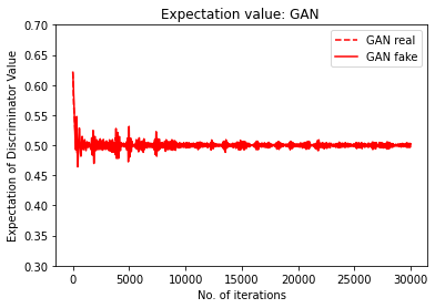
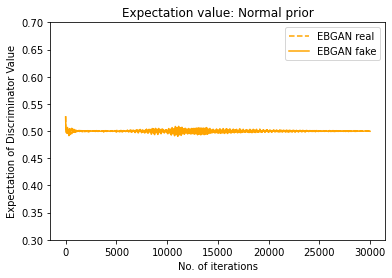
Figure S1: Empirical means of $D_{\theta_{d}^{(t)}}(x_{i})$ and $D_{\theta_{d}^{(t)}}(\tilde{x}_{i})$ produced by (a) GAN and (b) EBGAN with a Gaussian prior along with iterations.

S3.2 A Mixture Gaussian Example: Additional Results

For this example, we have tried the choice $\phi_{3}(D)=\log(D)$ of non-saturating GAN. Under this non-saturating setting, the game is no longer of the minimax style. However, it helps to overcome the gradient vanishing issue suffered by the minimax GAN. Figure S2 shows the empirical means $\mathbb{E}(D_{\theta_{d}^{(t)}}(x_{i}))$ and $\mathbb{E}(D_{\theta_{d}^{(t)}}(\tilde{x}_{i}))$ produced by different methods along with iterations. The non-saturating GAN and Lipschitz GAN still failed to converge to the Nash equilibrium, but BGAN and ProbGAN nearly converged after about 2000 iterations. In contrast, EBGAN still worked very well: It can converge to the Nash equilibrium in either case, with or without a Lipschitz penalty.

Figure S3 shows the plots of component recovery from the fake data. It indicates that EBGAN has recovered all 10 components of the real data in either case, with or without a Lipschitz penalty. Both ProbGAN and BGAN worked much better with this non-saturating choice than with the minimax choice of $\phi_{3}$: The ProbGAN has even recovered all 10 components, although the coverage area is smaller than that by EBGAN; and BGAN just had one component missed in recovery. The non-saturating GAN and Lipschitz GAN still failed for this example, which is perhaps due to the the model collapse issue. Using a single generator is hard to generate data following a multi-modal distribution.

(a)	(b)	(c)
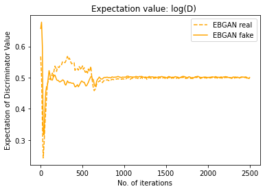
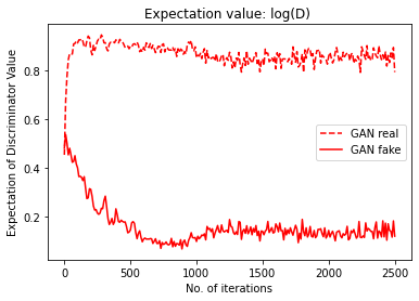
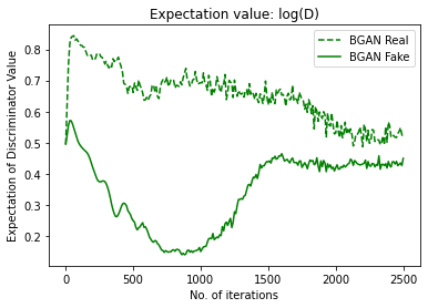
(d)	(e)	(f)

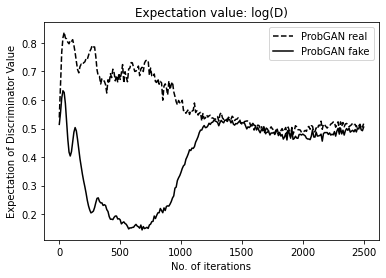
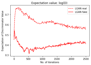
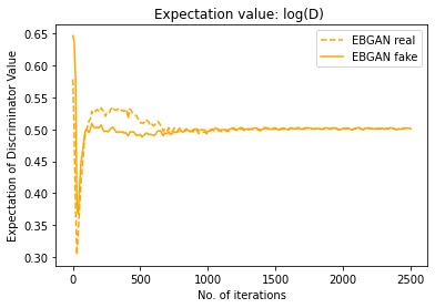
Figure S2: Nash equilibrium convergence plots with $\phi_{3}(D)=\log(D)$, which compare the empirical means of $D_{\theta_{d}^{(t)}}(x_{i})$ and $D_{\theta_{d}^{(t)}}(\tilde{x}_{i})$ produced by different methods along with iterations: (a) EBGAN with $\lambda=0$, (b) non-saturating GAN, (c) BGAN, (d) ProbGAN, (e) Lipschitz GAN, and (f) EBGAN with a Lipschitz penalty.

(a)	(b)	(c)
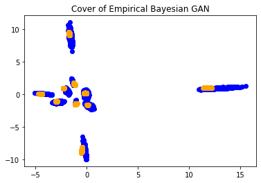
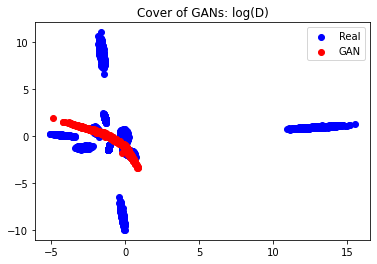
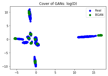
(e)	(e)	(f)

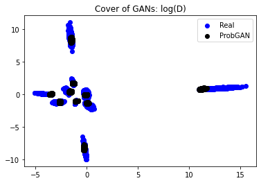
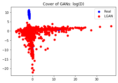
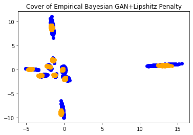
Figure S3: Component recovery plots produced by different methods with $\phi_{3}(D)=\log(D)$: (a) EBGAN with $\lambda=0$, (b) non-saturating GAN, (c) BGAN, (d) ProbGAN, (e) Lipschitz GAN, and (f) EBGAN with a Lipschitz penalty.

S3.3 Image Generation: HMNIST

We compared GAN and EBGAN on another real data problem, the HAM10000 (“Human Against Machine with 10000 training images”) dataset, which is also known as HMNIST and available at https://www.kaggle.com/kmader/skin-cancer-mnist-ham10000. The dataset consists of a total of 10,015 dermatoscopic images of skin lesions classified to seven types of skin cancer. Unlike other benchmark computer vision datasets, HMNIST has imbalanced group sizes. The largest group size is 6705, while the smallest one is 115, which makes it hard for conventional GAN training algorithms.

Our results for the example are shown in Figure S4, which indicates again that the EBGAN outperforms the GAN. In particular, the GAN is far from the 0.5-0.5 convergence, while EBGAN can achieve it. In terms of images generated by the two methods, it is clear that GAN suffers from a mode collapse issue; many images generated by it have a similar pattern even, e.g., those shown in the cells (1,4), (2,1), (4,1), (4,5), (5,2), (5,5) and (6,2) share a similar pattern. In contrast, the images generated by EBGAN show a clear clustering structure; each row corresponds to one different pattern.

(a)	(b)
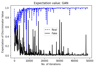
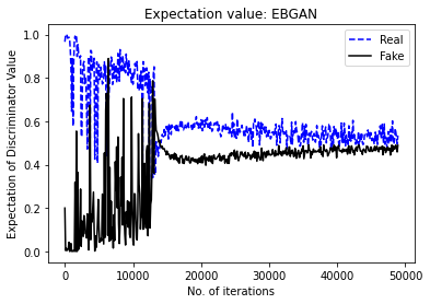
(c)	(d)
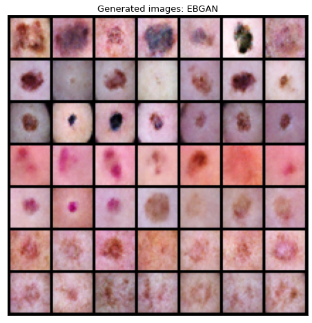
(e)	(f)

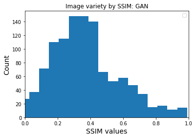
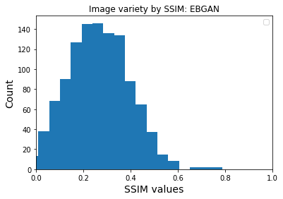
Figure S4: Results for the HMNIST example: (a) convergence plot of GAN; (b) convergence plot of EBGAN; (c) images generated by GAN; (d) images generated by EBGAN; (e) histograms of SSIMs for the images shown in plot (c) ; and (f) histograms of SSIMs for the images shown in plot (d).

Since the clusters in the dataset are imbalanced, the IS score does not work well for measuring the quality of the generated images. To tackle this issue, we calculated the structural similarity index measure (SSIM) Wang et al. (2004) for each pair of the images shown in Figure S4(c) and those shown in Figure S4(d), respectively. SSIM is a metric that measures the similarity between two images; it takes a value of 1 if two images are identical. Figure S4(e) & (f) shows the histograms of SSIMs for the images shown in Figure S4(c) & (d), respectively. The comparison shows clearly that the images generated by EBGAN have a larger diversity than those by GAN.

S3.4 Conditional Independence Tests

Conditional independence is a fundamental concept in graphical modeling (Lauritzen, 1996) and causal inference (Pearl, 2009) for multivariate data. Conditional independence tests have long been studied in statistics, which are to test the hypotheses

$$H_{0}:\ X\rotatebox[origin={c}]{90.0}{$\models$}Y|Z\quad versus\quad H_{1}:\ X\centernot\rotatebox[origin={c}]{90.0}{$\models$}Y|Z,$$

where $X\in\mathbb{R}^{d_{x}}$, $Y\in\mathbb{R}^{d_{y}}$ and $Z\in\mathbb{R}^{d_{z}}$. For the case that the variables are discrete and the dimensions are low, the Pearson $\chi^{2}$-test and the likelihood ratio tests are often used. For the case that the variables are Gaussian and linearly dependent, one often conducts the test using the partial correlation coefficient or its equivalent measure, see e.g., Spirtes et al. (1993) and Liang et al. (2015). However, in real-life situations, the normality and linear dependence assumptions are often not satisfied and thus nonparametric conditional independence tests are required. An abundance of such type of tests have been developed in the literature, e.g., permutation-based tests (Doran et al., 2014; Berrett et al., 2019), kernel-based tests (Zhang et al., 2012; Strobl et al., 2019), classification or regression-based tests (Sen et al., 2017; Zhang et al., 2017), and knockoff tests (Candès et al., 2018). Refer to Li and Fan (2019) for an overview.

As pointed out in Li and Fan (2019), the existing nonparametric conditional independence tests often suffer from the curse of dimensionality in the confounding vector $Z$; that is, the tests may be ineffective when the sample size is small, since the accumulation of spurious correlations from a large number of variables in $Z$ makes it difficult to discriminate between the hypotheses. As a remedy to this issue, Bellot and van der Schaar (2019) proposed a generative conditional independent test (GCIT) based on GAN. The method belongs to the class of nonparametric conditional independence tests and it consists of three steps: (i) simulating samples $\tilde{X}_{1},\ldots,\tilde{X}_{M}\sim q_{H_{0}}(X)$ under the null hypothesis $H_{0}$ via GAN, where $q_{H_{0}}(X)$ denotes the distribution of $X$ under $H_{0}$; (ii) defining an appropriate test statistic $\varrho(\cdot)$ which captures the $X$-$Y$ dependency in each of the samples $\{(\tilde{X}_{1},Y,Z),(\tilde{X}_{2},Y,Z),\ldots,(\tilde{X}_{M},Y,Z)\}$; and (iii) calculating the $p$-value

$$\widehat{p}=\frac{\sum_{m=1}^{M}\bf{1}\left\{\varrho(\tilde{X}_{m},Y,Z)>\varrho(X,Y,Z)\right\}}{M},$$ (S3.22)

which can be made arbitrarily close to the true probability

$$\mathbb{E}_{\tilde{X}\sim q_{H_{0}}(X)}\bf{1}\left\{\varrho(\tilde{X},Y,Z)\geq\varrho(X,Y,Z)\right\}$$

by sampling a large number of samples $\tilde{X}$ from $q_{H_{0}}(X)$. Bellot and van der Schaar (2019) proved that this test is valid and showed empirically that it is robust with respect to the dimension of the confounding vector $Z$. It is obvious that the power of the GCIT depends on how well the samples $\{\tilde{X}_{1},\tilde{X}_{2},\ldots,\tilde{X}_{m}\}$ approximate the distribution $q_{H_{0}}(X)$.

S3.4.1 Simulation Studies

To show that EBGAN improves the testing power of GCIT, we consider a simulation example taken from Bellot and van der Schaar (2019) for testing the hypotheses:

$$\begin{split}H_{0}:&\quad X=f_{1}(A_{x}Z+\epsilon_{x}),\quad Y=f_{2}(A_{y}Z+\epsilon_{y}),\\ H_{1}:&\quad X=f_{1}(A_{x}Z+\epsilon_{x}),\quad Y=f_{3}(\alpha A_{xy}X+A_{y}Z+\epsilon_{y}),\end{split}$$

where the matrix dimensions of $A_{(\cdot)}$ are such that $X$ and $Y$ are univariate. The entries of $A_{(\cdot)}$ as well as the parameter $\alpha$ are randomly drawn from Unif$[0,1]$, and the noise variables $\epsilon_{(\cdot)}$ are Gaussian with mean 0 and variance 0.025. Three specific cases are considered in the simulation:

• Case 1. Multivariate Gaussian: $f_{1}$, $f_{2}$ and $f_{3}$ are identity functions, $Z\sim\mathcal{N}(0,I_{d_{z}})$, which result in multivariate Gaussian data and linear dependence under $H_{1}$.

• Case 2. Arbitrary relationship: $f_{1}$, $f_{2}$ and $f_{3}$ are randomly sampled from $\{\tanh(x),\exp(-x)$, $x^{2}\}$, $Z\sim N(0,I_{d_{z}})$, which results in more complex distributions and variable dependencies. It resembles the complexities we can expect in real applications.

• Case 3. Arbitrary relationships with a mixture $Z$ distribution:

  $$\begin{split}H_{0}:&\quad X=\{f_{1,a}(A_{x}Z_{a}+\epsilon_{x}),f_{1,b}(A_{x}Z_{b}+\epsilon_{x})\},\quad Y=f_{2}(A_{y}Z+\epsilon_{y}),\\ H_{1}:&\quad X=\{f_{1,a}(A_{x}Z_{a}+\epsilon_{x}),f_{1,b}(A_{x}Z_{b}+\epsilon_{x})\},\quad Y=f_{3}(\alpha A_{xy}X+A_{y}Z+\epsilon_{y}),\end{split}$$

  where $Z_{a}\sim\mathcal{N}(1_{d},I_{d})$, $Z_{b}\sim\mathcal{N}(-1_{d},I_{d})$, $Z_{a},Z_{b}\in\mathbb{R}^{\frac{n}{2}\times d}$, $Z=(Z_{a}^{T},Z_{b}^{T})^{T}$, $f_{1,a}$, $f_{1,b}$, $f_{2}$ and $f_{3}$ are randomly sampled from $\{\tanh(x),\exp(-x),x^{2}\}$ and $f_{1,a}\neq f_{1,b}$.

For each case, we simulated 100 datasets under $H_{1}$, where each dataset consisted of $150$ samples. Both GAN and EBGAN were applied to this example with the randomized dependence coefficient (Lopez-Paz et al., 2013) used as the test statistic $\varrho(\cdot)$. Here GAN was trained as in Bellot and van der Schaar (2019) with the code available at https://github.com/alexisbellot/GCIT. In GAN, the objective function of the generator was regularized by a mutual information which encourages to generate samples $\tilde{X}$ as independent as possible from the observed variables $X$ and thus enhances the power of the test. The EBGAN was trained in a plain manner without the mutual information term included in $\mathcal{J}(\theta_{d};\theta_{g})$. Detailed settings of the experiments were given in the supplement. In addition, two kernel-based methods, KCIT (Zhang et al., 2012) and RCoT (Strobl et al., 2019), were applied to this example for comparison.

(a)

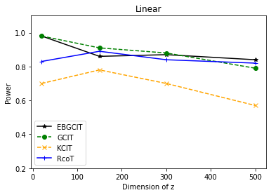
(b)

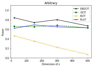
(c)

Figure S5: Generative conditional independence tests with GAN (denoted by GCIT) and EBGAN (denoted by EBGCIT): (a) Power curve for Case 1; (b) Power curve for Case 2 ; (c) Power curve for Case 3

Figure S5 summarizes the results of the experiments. For case 1, EBGAN, GAN and RCoT are almost the same, and they all outperform KCIT. For case 2 and case 3, EBGAN outperforms the other three methods significantly. Note that, by Bellot and van der Schaar (2019), GAN represents the state-of-the-art method for high-dimensional nonparametric conditional independence tests. For similar examples, Bellot and van der Schaar (2019) showed that GAN significantly outperformed the existing statistical tests, including the kernel-based tests (Zhang et al., 2012; Strobl et al., 2019), knockoff-based test (Candès et al., 2018), and classification-based test (Sen et al., 2017).

S3.4.2 Identifications of Drug Sensitive Mutations

As a real data example, we applied EBGAN to identification of genetic mutations that affect response of cancer cells to an anti-cancer drug. This helps cancer clinics, as the treatment for a cancer patient can strongly depend on the mutation of his/her genome (Garnett et al., 2012) in precision medicine. We used a sub-dataset of Cancer Cell Line Encyclopedia (CCLE), which relates the drug response of PLX4720 with 466 genetic mutations. The dataset consists of 474 cell lines. Detailed settings of the experiment were given in the supplement.

Table S1 shows the mutations identified by EBGAN at a significance level of 0.05, where the dependency of the drug response on the first 12 mutations has been validated by the existing literature at PubMed. Since PLX4720 was designed as a BRAF inhibitor, the low p-values of BRAF.MC, BRAF.V600E and BRAF confirm the validity of the proposed test. EBGAN also identified MYC as a drug sensitive mutation, but which was not detected via GAN in Bellot and van der Schaar (2019). Our finding is validated by Singleton et al. (2017), which reported that BRAF mutant cell lines with intrinsic resistance to BRAF rapidly upregulate MYC upon treatment of PLX4720. CRKL is another mutation identified by EBGAN but not by GAN, and this finding can be validated by the experimental results reported in Tripathi et al. (2020).

Table S1: Genetic experiment results: Each cell gives the p-value indicating the dependency between a mutation and drug response, where the superscript ^- indicates that the dependency of drug response on the mutation has not yet been validated in the literature.

BRAF.MC IRAK1 BRAF.V600E BRAF HIP1 SRPK3 MAP2K4 FGR 0.001 0.002 0.003 0.003 0.004 0.012 0.014 0.014 PRKD1 CRKL MPL MYC MTCP1^- ADCK2^- RAD51L1^- 0.015 0.016 0.027 0.037 0.011 0.037 0.044

S3.5 Nonparametric Clustering

This section gives details for different datasets we tried.

S3.5.1 Two-Circle Problem

The most notorious example for classical clustering methods is the two-circle problem. The dataset is generated as follows:

$$\begin{split}Z_{i}=(z_{1i},z_{2i}&),\quad\rm{where}\quad z_{1i},z_{2i}\overset{\textit{iid}}{\sim}Unif[-1,1],\quad i=1,\dots,1000;\\ \mbox{Inner Circle}&:0.25*\left(\frac{z_{1i}}{\sqrt{z_{1i}^{2}+z_{2i}^{2}}},\frac{z_{2i}}{\sqrt{z_{1i}^{2}+z_{2i}^{2}}}\right)+\epsilon,\quad i=1,\dots,500;\\ \mbox{Outer Circle}&:\left(\frac{z_{1i}}{\sqrt{z_{1i}^{2}+z_{2i}^{2}}},\frac{z_{2i}}{\sqrt{z_{1i}^{2}+z_{2i}^{2}}}\right)+\epsilon,\quad i=501,\dots,1000,\end{split}$$ (S3.23)

where $\epsilon\sim\mathcal{N}(0,0.05^{2}I_{2})$. For this example, the K-means and agglomerative clustering methods are known to fail to detect the inner circle unless the data are appropriately transformed; DBSCAN is able to detect the inner circle, but it is hard to apply to other high-dimensional problems due to its density estimation-based nature.

For a simulated dataset, each of the methods, including K-means, agglomerative, DBSCAN, Cluster GAN and Cluster EBGAN, was run for 100 times with different initializations. Figure S6 shows the histogram of the adjust Rand index (ARI) (Rand, 1971) values obtained in those runs. It indicates that K-means, agglomerative and DBSCAN produced the same clustering results in different runs, while Cluster GAN and Cluster EBGAN produced different ones in different runs. In particular, the ARI values resulted from Cluster GAN are around 0, whereas those from Cluster EBGAN are around 1.0. Figure S7 shows some clustering results produced by these methods.

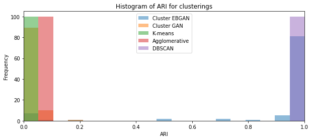
Figure S6: Histogram of ARI produced by different methods: Cluster EBGAN, Cluster GAN, K-means, Agglomerative, and DBSCAN.

(a)	(b)	(c)	(d)
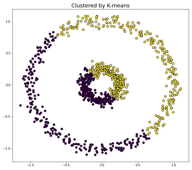
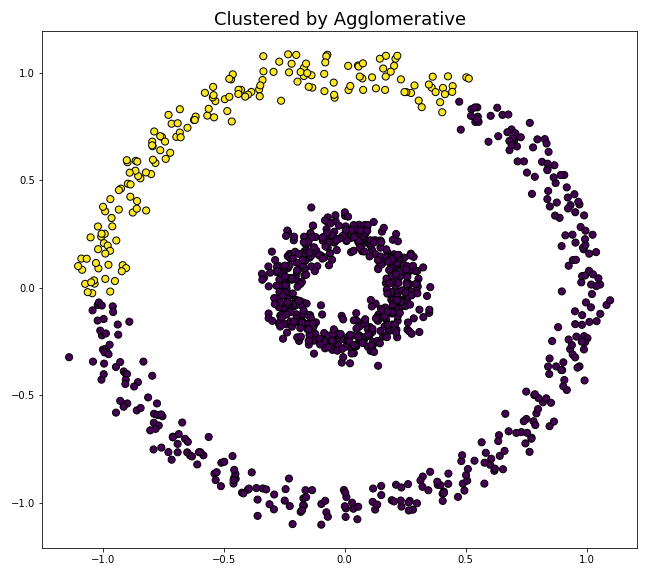
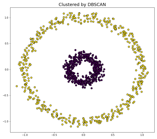
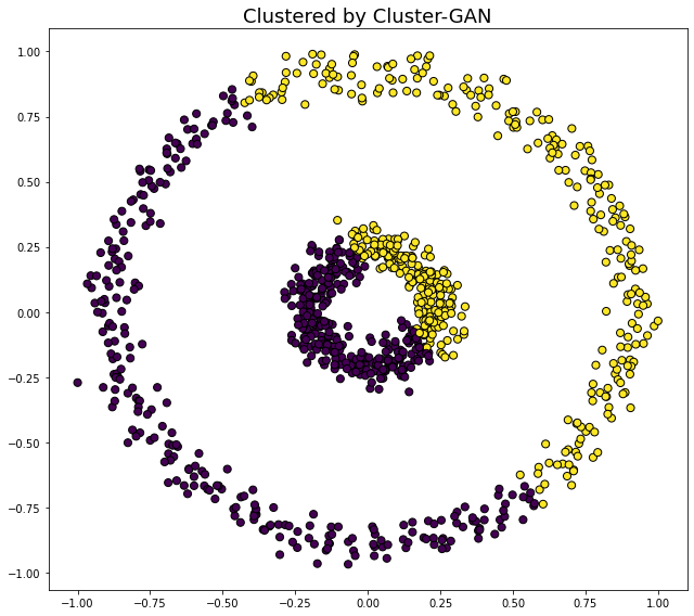
(e)	(f)	(g)	(h)

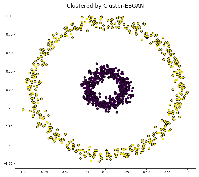
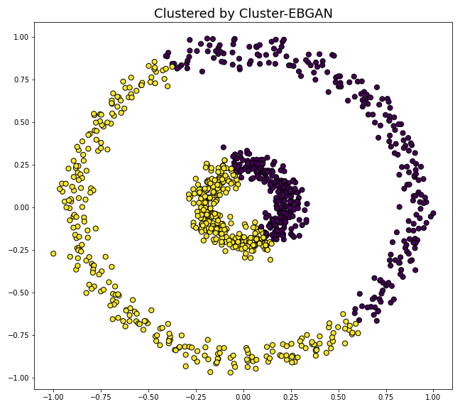
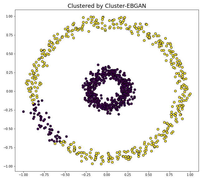
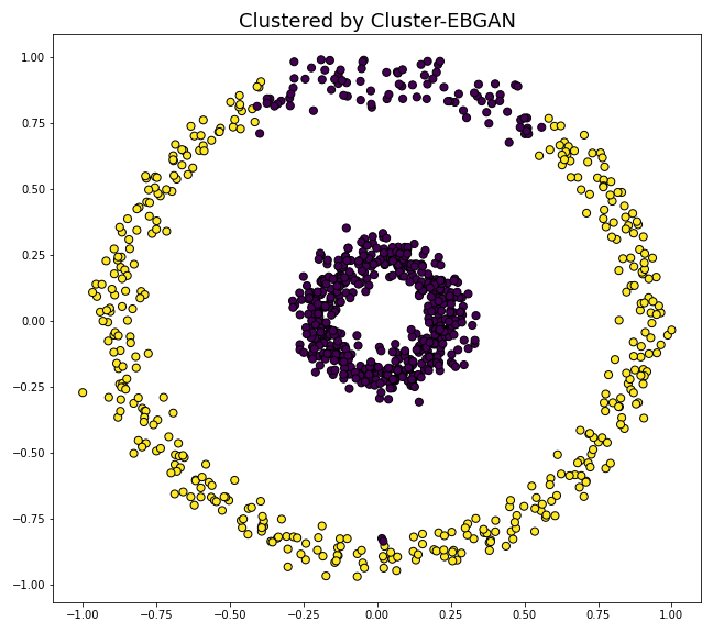
Figure S7: (a) K-means clustering, (b) Agglomerative clustering, (c) DBSCAN, (d) Cluster-GAN, (e)-(h) Cluster-EBGAN in different runs.

Figure S6 and Figure S7 indicate that DBSCAN can constantly detect the inner circle; Cluster EBGAN can detect the inner circle in nearly 80% of the runs; while K-means, agglomerative, and Cluster GAN failed to detect the inner circle. The comparison with Cluster GAN indicates that Cluster EBGAN has made a significant improvement in GAN training.

Iris

This is a classical clustering example. It contains the data for 50 flowers from each of three species - Setosa, Versicolor and Virginica. The dataset is available at https://archive.ics.uci.edu/ml/datasets/iris, which gives the measurements of the variables sepal length and width and petal length and width for each of the flowers. Table 2 summarizes the performance of different methods on the dataset. Other than ARI, the cluster purity is also calculated as a measure of the quality of clusters. Suppose that the data consists of $K$ clusters and each cluster consists of $n_{k}$ observations denoted by $\{x_{k}^{j}\}_{j=1}^{n_{k}}$. If the data were grouped into $M$ clusters, then the cluster purity is defined by

$$\frac{\sum_{k=1}^{K}\max\{\sum_{j=1}^{n_{k}}1(\mathcal{E}_{2}(x_{k}^{j})=l):l=1,2,\ldots,M\}}{n_{1}+\dots+n_{K}},$$

which measures the percentage of the samples being correctly clustered. Both the measures, ARI and cluster purity, have been used in Mukherjee et al. (2019) for assessing the performance of Cluster GAN. The comparison shows that Cluster EBGAN significantly outperforms Cluster GAN and classical clustering methods in both ARI and cluster purity.

Seeds

The dataset is available at https://archive.ics.uci.edu/ml/datasets/seeds. The examined group comprised kernels belonging to three different varieties of wheat: Kama, Rosa and Canadian, 70 elements each, randomly selected for the experiment. Seven geometric parameters of wheat kernels were measured, including area, perimeter, compactness, length, width, asymmetry coefficient, and length of kernel groove. Table 2 summarizes the performance of different methods on the dataset. The comparison indicates that Cluster EBGAN significantly outperforms others in both ARI and cluster purity. For this dataset, DBSCAN is not available any more, as performing density estimation in a 7-dimensional space is hard.

MNIST

The MNIST dataset consists of 70,000 images of digits ranging from 0 to 9. Each sample point is a $28\times 28$ grey scale image. Figure S8 compares the images generated by Cluster GAN and Cluster EBGAN, each representing the best result achieved by the corresponding method in 5 independent runs. It is remarkable that Cluster EBGAN can generate all digits from 0 to 9 and there is no confusion of digits between different generators. However, Cluster GAN failed to generate the digit 1 and confused the digits 4 and 9. Table 2 summarizes the performance of different methods, which indicates again the superiority of the Cluster EBGAN over Cluster GAN and classical nonparametric methods.

(a)	(b)

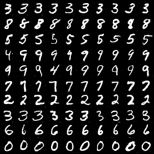
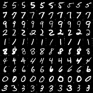
Figure S8: Images generated by (a) Cluster GAN and (b) Cluster EBGAN, where each row corresponds to a different $z_{c}$ index vector.

Appendix S4 Experimental Settings

In all training with the Adam algorithm (Kingma et al., 2015), we set the tuning parameters $(\alpha_{1},\alpha_{2})=(0.5,0.999)$. In this paper, all the deep convolutional GANs (DCGANs) were trained using the Adam algorithm.

For Algorithm 1 (of the main text), the step size is chosen in the form $w_{t}=c_{1}(t+c_{2})^{-\zeta_{1}}$, and the momentum smoothing factor $\alpha$ is re-denoted by $\alpha_{1}$ in Tables S3-S5. A constant learning rate $\epsilon$ and a constant momentum biasing factor $\rho=1$.

S4.1 A Gaussian Example

Table S2 gives the parameter settings of GAN and EBGAN for the Gaussian example.

Table S2: Parameter settings for the 2D Gaussian dataset with $\phi_{3}(D)=log(D)$

Method	Learning rate		$\alpha_{1}$	$\alpha_{2}$	$\rho$
	Discriminator($\omega_{t}$)	Generator($\epsilon_{t}$)
GAN	0.00002	0.0002	0.5	0.999
EBGAN	$(c_{1},c_{2},\zeta_{1})=(1,1000,0.75)$	0.01	0.9		1

S4.2 A Mixture Gaussian Example

Tables S3 and S4 give the parameter settings of different methods for the minimax and non-saturating cases, respectively. For EBGAN, we set $\tau=0.01$.

Table S3: Parameter settings for the synthetic dataset: the minimax case with $\phi_{3}(D)=-\log(1-D)$

Method Learning rate $\alpha_{1}$ $\alpha_{2}$ $\rho$ $\lambda(\text{Lipshitz})$ Discriminator Generator GAN 0.0002 0.0002 0.5 0.999 BGAN 0.001 0.001 0.9 Probgan 0.0005 0.0005 0.5 EBGAN $(c_{1},c_{2},\zeta_{1})=(1,1000,0.75)$ 0.5 0.9 1 Lipshitz-GAN 0.0002 0.0002 0.5 0.999 5 Lipshitz-EBGAN $(c_{1},c_{2},\zeta_{1})=(1,1000,0.75)$ 0.5 0.9 1 5

Table S4: Parameter settings for the synthetic dataset: the non-saturating case with $\phi_{3}(D)=\log(D)$

Method Learning rate $\alpha_{1}$ $\alpha_{2}$ $\rho$ $\lambda(\text{Lipshitz})$ Discriminator Generator GAN 0.0002 0.0002 0.5 0.999 BGAN 0.001 0.001 0.9 Probgan 0.0005 0.0005 0.9 EBGAN $(c_{1},c_{2},\zeta_{1})=(1,1000,0.75)$ 0.5 0.9 1 Lipshitz-GAN 0.0002 0.0002 0.5 0.999 5 Lipshitz-EBGAN $(c_{1},c_{2},\zeta_{1})=(1,1000,0.75)$ 0.5 0.9 1 5

S4.3 Fashion MNIST

The network structures of all models are typical DCGAN style. We set the mini-batch size to 300, set the total number of epochs to 200, and set the dimension of $z_{n}$ to 10. For training the inception model, we used Adam with a learning rate of $0.0003$, $(\alpha_{1},\alpha_{2})=(0.9,0.999)$, a mini-batch size of 50, and $5$ epochs. After training, the prediction accuracy on the test data set was $0.9304$. Table S5 gives the parameter settings used by different methods. And we set $\zeta_{2}=\frac{1}{40}$ for EBGAN referring to Kim et al. (2022). In addition, we set $\tau=0.001$ for EBGAN, and set $k_{g}=10$ for EBGAN, BGAN and ProbGAN.

Table S5: Parameter settings for the Fashion MNIST

Method Learning rate $\alpha_{1}$ $\alpha_{2}$ $\rho$ Discriminator Generator GAN 0.0002 0.0002 0.5 0.999 BGAN 0.005 0.005 0.9 ProbGAN 0.005 0.005 0.9 EBGAN-KL $(c_{1},c_{2},\zeta_{1})=(0.5,250,1)$ with Adam 0.01 0.9 1 EBGAN-Gaussian $(c_{1},c_{2},\zeta_{1})=(1,500,1)$ with Adam 0.01 0.9 1

Table S6: Model structure of EBGAN for Fashion MNIST

Generator	Discriminator
4$\times$ 4 conv, 512 stride 2 ReLU	4$\times$ 4 conv, 64 stride 2 pad 1 LReLU
3$\times$ 3 conv, 256 stride 2 pad 1 ReLU	4$\times$ 4 conv, 128 stride 2 pad 1 LReLU
4$\times$ 4 conv, 128 stride 2 pad 1 ReLU	3$\times$ 3 conv, 256 stride 2 pad 1 LReLU
$4\times 4$ upconv 64 stride 2 pad 1 Tanh	4$\times$ 4 conv, 512 stride 2 LReLU

S4.4 HMNIST

We set the latent dimension as 20, and use the normal prior $N(0,\frac{1}{80})$ on 7 generator parameters with temperature $\tau=0.001$, with 200 batch size. Other parameter settings and the model structure are given in Table S7 and Table S8, respectively.

Table S7: Parameter settings for the HMNIST

Method Learning rate $\alpha_{1}$ $\alpha_{2}$ $\rho$ Discriminator Generator GAN 0.0002 0.0002 0.5 0.999 EBGAN-Gaussian $(c_{1},c_{2},\zeta_{1})=(0.05,250,1)$ with Adam 0.001 0.9 1

Table S8: Model structure of EBGAN for HMNIST

Generator	Discriminator
4$\times$ 4 conv, 512 stride 2 ReLU	4$\times$ 4 conv, 64 stride 2 pad 1 LReLU
3$\times$ 3 conv, 256 stride 2 pad 1 ReLU	4$\times$ 4 conv, 128 stride 2 pad 1 LReLU
4$\times$ 4 conv, 128 stride 2 pad 1 ReLU	3$\times$ 3 conv, 256 stride 2 pad 1 LReLU
$4\times 4$ upconv 64 stride 2 pad 1 Tanh	4$\times$ 4 conv, 512 stride 2 LReLU

S4.5 Conditional independence test

Simulated Data

The network structures of all models we used are the same as in Bellot and van der Schaar (2019). In short, the generator network has a structure of $(d+d/10)-(d/10)-1$ and the discriminator network has a structure of $(1+d)-(d/10)-1$, where $d$ is the dimension of the confounding vector $Z$. All experiments for GCIT were implemented with the code given at https://github.com/alexisbellot/GCIT/blob/master/GCIT.py. For the functions $\phi_{1}$, $\phi_{2}$ and $\phi_{3}$, the nonsaturating settings were adopted, i.e., we set $(\phi_{1},\phi_{2},\phi_{3})=(\log x,\log(1-x),\log x)$. For both cases of the synthetic data, EBGAN was run with a mini-batch size of 64, Adam optimization was used with learning rate 0.0001 for discriminator. A prior $p_{g}=N(0,100I_{p})$, $p$ for dimension of parameters, and a constant learning rate of 0.005 were used for the generator. Lastly, we set $\tau=1$. Each run consisted of 1000 iterations for case 1, case 2 and case 3. KCIT and RcoT were run by R-package at https://github.com/ericstrobl/RCIT.

CCLE Data

For the CCLE dataset, EBGAN was run for 1000 iterations and $(c_{1},c_{2},\eta_{1},\alpha_{1})=(1,1000,0.75,0.9)$ was used. Other parameters were set as above.

S4.6 Nonparametric Clustering

Two Circle

We set the dimension of $z_{n}$ to 3, set $(\beta_{n},\beta_{c})=(0.1,0.1)$, set the mini-batch size to 500, and set a constant learning rate of 0.05 with $\tau=1$ for the generator. For optimization of the discriminator, we used Adam and set $(\alpha_{1},\alpha_{2})=(0.5,0.9)$ with a constant learning rate of 0.1. The total number of epochs was set to 2000.

Table S9: Model structure of Cluster-GAN and Cluster-EBGAN for two-circle data

Generator	Encoder	Discriminator
FC 20 LReLU	FC 20 LReLU	FC 30 LReLU
FC 20 LReLU	FC 20 LReLU	FC 30 LReLU
FC 2 linear Tanh	FC 5 linear	FC 1 linear

Iris

For the iris data, we used a simple feed-forward network structure for Cluster GAN and Cluster EBGAN. We set the dimension of $z_{n}$ to 20, set $(\beta_{n},\beta_{c})=(10,10)$, set the mini-batch size to 32, and set a constant learning rate of 0.01 for the generator with $\tau=1$. For optimization of the discriminator, we used Adam and set $(\alpha_{1},\alpha_{2})=(0.5,0.9)$ with a learning rate of 0.0001. The hyperparameters of Cluster-GAN is set to the default values.

Table S10: Model structure of Cluster-GAN and Cluster-EBGAN for Iris

Generator	Encoder	Discriminator
FC 5 LReLU	FC 5 LReLU	FC 5 LReLU
FC 5 LReLU	FC 5 LReLU	FC 5 LReLU
FC 4 linear Sigmoid	FC 23 linear	FC 1 linear

Seeds

For the seeds data, we used a simple feed-forward network structure for Cluster-GAN and Cluster-EBGAN. We set the dimension of $z_{n}$ to 20, set $(\beta_{n},\beta_{c})=(5,5)$, set the mini-batch size to 128, and set a constant learning rate of 0.01 for generator with $\tau=0.0001$. For optimization of the discriminator, we used Adam and set $(\alpha_{1},\alpha_{2})=(0.5,0.9)$ with a learning rate of 0.005. The hyperparameters of Cluster-GAN is set to the default values.

Table S11: Model structure of Cluster-GAN and Cluster-EBGAN for Seeds

Generator	Encoder	Discriminator
FC 20 LReLU	FC 20 LReLU	FC 100 LReLU
FC 20 LReLU	FC 20 LReLU	FC 100 LReLU
FC 7 linear Tanh	FC 23 linear	FC 1 linear

MNIST

For Cluster GAN, our implementation is based on the code given at https://github.com/zhampel/clusterGAN, with a a small modification on Encoder. The Structures of the generator, encoder and discriminator are given as follow. Cluster GAN was run with the same parameter setting as given in the original work Mukherjee et al. (2019).

Table S12: Model structure of ClusterGAN for MNIST data

Generator Encoder Discriminator FC 1024 ReLU BN 4$\times$ 4 conv, 64 stride 2 LReLU 4$\times$ 4 conv, 64 stride 2 LReLU FC $7\times 7\times 128$ ReLU BN 4$\times$ 4 conv, 128 stride 2 LReLU 4$\times$ 4 conv, 64 stride 2 LReLU $4\times 4$ upconv 64 stride 2 ReLU BN 4$\times$ 4 conv, 256 stride 2 LReLU FC1024 LReLU $4\times 4$ upconv 1 stride 2 Sigmoid FC 1024 LReLU FC 1 linear FC 40

For Cluster EBGAN, to accelerate computation, we used the parameter sharing strategy as in Hoang et al. (2018), where all generators share the parameters except for the first layer. We set the dimension of $z_{n}$ to 5, $(c_{1},c_{2},\eta_{1},\alpha_{1})=(40,10000,0.75,0.9)$, set the mini-batch size to 100, and set a constant learning rate of $0.005$ for the generator. For the functions $\phi_{1}$, $\phi_{2}$ and $\phi_{3}$, the non-saturating settings were adopted, i.e., we set $(\phi_{1},\phi_{2},\phi_{3})=(\log x,\log(1-x),\log x)$.

Table S13: Model structure of ClusterEBGAN for MNIST simulation

Generator Encoder Discriminator 4$\times$ 4 conv, 512 stride 2 ReLU 4$\times$ 4 conv, 64 stride 2 LReLU 4$\times$ 4 conv, 64 stride 2 LReLU 3$\times$ 3 conv, 128 stride 2 pad 1 ReLU 4$\times$ 4 conv, 128 stride 2 LReLU 4$\times$ 4 conv, 64 stride 2 LReLU 4$\times$ 4 conv, 64 stride 2 pad 1 ReLU 4$\times$ 4 conv, 256 stride 2 LReLU FC1024 LReLU $4\times 4$ upconv 1 stride 2 pad 1 Sigmoid FC 1024 LReLU FC 1 linear FC 30

References

- Andrieu et al. (2005) Andrieu, C., E. Moulines, and P. Priouret (2005). Stability of stochastic approximation under verifiable conditions. SIAM Journal on Control and Optimization 44(1), 283–312.
- Arjovsky et al. (2017) Arjovsky, M., S. Chintala, and L. Bottou (2017, 06–11 Aug). Wasserstein generative adversarial networks. In D. Precup and Y. W. Teh (Eds.), Proceedings of the 34 th International Conference on Machine Learning (ICML), Volume 70 of PMLR, International Convention Centre, Sydney, Australia, pp. 214–223.
- Arnold and Press (1989) Arnold, B. C. and S. J. Press (1989). Compatible conditional distributions. Journal of the American Statistical Association 84(405), 152–156.
- Arora et al. (2017) Arora, S., R. Ge, Y. Liang, T. Ma, and Y. Zhang (2017). Generalization and equilibrium in generative adversarial nets (GANs). In ICML, pp. 224–232.
- Bellot and van der Schaar (2019) Bellot, A. and M. van der Schaar (2019). Conditional independence testing using generative adversarial networks. In NeurIPS, pp. 2202–2211.
- Benveniste et al. (1990) Benveniste, A., M. Métivier, and P. Priouret (1990). Adaptive Algorithms and Stochastic Approximations. Springer.
- Berrett et al. (2019) Berrett, T., Y. Wang, R. Barber, and R. Samworth (2019, 10). The conditional permutation test for independence while controlling for confounders. Journal of the Royal Statistical Society: Series B (Statistical Methodology) 82.
- Binkowski et al. (2018) Binkowski, M., D. J. Sutherland, M. Arbel, and A. Gretton (2018). Demystifying MMD GANs. In ICLR.
- Candès et al. (2018) Candès, E., Y. Fan, L. Janson, and J. Lv (2018). Panning for gold: ‘model-x’ knockoffs for high dimensional controlled variable selection. Journal of the Royal Statistical Society: Series B (Statistical Methodology) 80(3), 551–577.
- Che et al. (2017) Che, T., Y. Li, A. P. Jacob, Y. Bengio, and W. Li (2017). Mode regularized generative adversarial networks. In ICLR.
- Chen et al. (2015) Chen, C., N. Ding, and L. Carin (2015). On the convergence of stochastic gradient mcmc algorithms with high-order integrators. In Advances in Neural Information Processing Systems, pp. 2278–2286.
- Chen and Zhu (1986) Chen, H. and Y. Zhu (1986). Stochastic approximation procedures with randomly varying truncations. Science in China Series A-Mathematics, Physics, Astronomy & Technological Science 29(9), 914–926.
- Chen et al. (2014) Chen, T., E. B. Fox, and C. Guestrin (2014). Stochastic gradient hamiltonian monte carlo. In ICML.
- Dempster et al. (1977) Dempster, A., N. Laird, and D. Rubin (1977). Maximum likelihood from incomplete data via the em algorithm. Journal of the Royal Statistical Society, Series B 39, 1–38.
- Deng et al. (2019) Deng, W., X. Zhang, F. Liang, and G. Lin (2019). An adaptive empirical bayesian method for sparse deep learning. NeurIPS 2019.
- Dong et al. (2023) Dong, T., P. Zhang, and F. Liang (2023). A stochastic approximation-langevinized ensemble kalman filter for state space models with unknown parameters. Journal of Computational and Graphical Statistics 32(2), 448–469.
- Doran et al. (2014) Doran, G., K. Muandet, K. Zhang, and B. Schölkopf (2014). A permutation-based kernel conditional independence test. In Proceedings of the Thirtieth Conference on Uncertainty in Artificial Intelligence, UAI’14, Arlington, Virginia, USA, pp. 132–141. AUAI Press.
- Dragomir et al. (2000) Dragomir, S., M. Scholz, and J. Sunde (2000). Some upper bounds for relative entropy and applications. Computers & Mathematics with Applications 39(9), 91–100.
- Gao et al. (2021) Gao, X., M. Gürbüzbalaban, and L. Zhu (2021). Global convergence of stochastic gradient hamiltonian monte carlo for nonconvex stochastic optimization: Nonasymptotic performance bounds and momentum-based acceleration. Operations Research.
- Gao et al. (2019) Gao, Y., Y. Jiao, Y. Wang, Y. Wang, C. Yang, and S. Zhang (2019). Deep generative learning via variational gradient flow. In ICML, pp. 2093–2101.
- Garnett et al. (2012) Garnett, M. J., E. J. Edelman, S. J. Heidorn, C. D. Greenman, A. Dastur, K. W. Lau, P. Greninger, I. R. Thompson, X. Luo, J. Soares, Q. Liu, F. Iorio, D. Surdez, L. Chen, R. J. Milano, G. R. Bignell, A. T. Tam, H. Davies, J. A. Stevenson, S. Barthorpe, S. R. Lutz, F. Kogera, K. Lawrence, A. McLaren-Douglas, X. Mitropoulos, T. Mironenko, H. Thi, L. Richardson, W. Zhou, F. Jewitt, T. Zhang, P. O’Brien, J. L. Boisvert, S. Price, W. Hur, W. Yang, X. Deng, A. Butler, H. G. Choi, J. W. Chang, J. Baselga, I. Stamenkovic, J. A. Engelman, S. V. Sharma, O. Delattre, J. Saez-Rodriguez, N. S. Gray, J. Settleman, P. A. Futreal, D. A. Haber, M. R. Stratton, S. Ramaswamy, U. McDermott, and C. H. Benes (2012, March). Systematic identification of genomic markers of drug sensitivity in cancer cells. Nature 483(7391), 570—575.
- Ghosh et al. (2018) Ghosh, A., V. Kulharia, V. Namboodiri, P. Torr, and P. Dokania (2018, 06). Multi-agent diverse generative adversarial networks. In CVPR, pp. 8513–8521.
- Goodfellow et al. (2014) Goodfellow, I., J. Pouget-Abadie, M. Mirza, B. Xu, D. Warde-Farley, S. Ozair, A. Courville, and Y. Bengio (2014). Generative adversarial nets. NIPS, 2672–2680.
- He et al. (2019) He, H., H. Wang, G.-H. Lee, and Y. Tian (2019). Probgan: Towards probabilistic gan with theoretical guarantees. ICLR.
- Hoang et al. (2018) Hoang, Q., T. D. Nguyen, T. Le, and D. Phung (2018). MGAN: Training generative adversarial nets with multiple generators. In ICLR.
- Kass et al. (1990) Kass, R. E., L. Tierney, and J. B. Kadane (1990). The validity of posterior expansions based on Laplace’s method. In S. Geisser, J. S. Hodges, S. J. Press, and A. ZeUner (Eds.), Bayesian and likelihood methods in statistics and econometrics: essays in honor of George A. Barnard, Volume 7, pp. 473–488. Amsterdam: North Holland.
- Kim et al. (2022) Kim, S., Q. Song, and F. Liang (2022). Stochastic gradient langevin dynamics with adaptive drifts. Journal of Statistical Computation and Simulation 92(2), 318–336.
- Kingma et al. (2015) Kingma, D. P., and J. L. Ba (2015). Adam: a method for stochastic optimization. In International Conference on Learning Representations.
- Kingma and Ba (2014) Kingma, D. and J. Ba (2014). Adam: A method for stochastic optimization. ICLR, 1–13.
- Kirkpatrick et al. (1983) Kirkpatrick, S., C. Gelatt, and M. Vecchi (1983). Optimization by simulated annealing. Science 220, 671–680.
- Lauritzen (1996) Lauritzen, S. (1996). Graphical Models. Clarendon Press.
- Li et al. (2016) Li, C., C. Chen, D. Carlson, and L. Carin (2016). Preconditioned stochastic gradient langevin dynamics for deep neural networks. In AAAI.
- Li and Fan (2019) Li, C. and X. Fan (2019, 12). On nonparametric conditional independence tests for continuous variables. Wiley Interdisciplinary Reviews: Computational Statistics 12.
- Liang et al. (2015) Liang, F., Q. Song, and P. Qiu (2015). An equivalent measure of partial correlation coefficients for high dimensional gaussian graphical models. Journal of the American Statistical Association 110, 1248–1265.
- Liu et al. (2021) Liu, Q., J. Xu, R. Jiang, and W. H. Wong (2021). Density estimation using deep generative neural networks. Proceedings of the National Academy of Sciences 118(15), e2101344118.
- Lopez-Paz et al. (2013) Lopez-Paz, D., P. Hennig, and B. Schölkopf (2013). The randomized dependence coefficient. In C. J. C. Burges, L. Bottou, M. Welling, Z. Ghahramani, and K. Q. Weinberger (Eds.), Advances in Neural Information Processing Systems, Volume 26, pp. 1–9. Curran Associates, Inc.
- Mao et al. (2017) Mao, X., Q. Li, H. Xie, R. Lau, W. Zhen, and S. Smolley (2017). Least squares generative adversarial networks. In ICCV, pp. 2813–2821.
- Morris (1983) Morris, C. N. (1983). Parametric empirical bayes inference: Theory and applications. Journal of the American Statistical Association 78(381), 47–55.
- Mukherjee et al. (2019) Mukherjee, S., H. Asnani, E. Lin, and S. Kannan (2019). Clustergan: Latent space clustering in generative adversarial networks. In AAAI, pp. 4610–4617. AAAI Press.
- Nowozin et al. (2016) Nowozin, S., B. Cseke, and R. Tomioka (2016). f-gan: Training generative neural samplers using variational divergence minimization. In NIPS.
- Pearl (2009) Pearl, J. (2009, 01). Causal inference in statistics: An overview. Statistics Surveys 3, 96–146.
- Pérez-Cruz (2008) Pérez-Cruz, F. (2008). Kullback-leibler divergence estimation of continuous distributions. 2008 IEEE International Symposium on Information Theory, 1666–1670.
- Raginsky et al. (2017) Raginsky, M., A. Rakhlin, and M. Telgarsky (2017). Non-convex learning via stochastic gradient langevin dynamics: a nonasymptotic analysis. In Conference on Learning Theory, pp. 1674–1703. PMLR.
- Rand (1971) Rand, W. M. (1971). Objective criteria for the evaluation of clustering methods. Journal of the American Statistical Association 66(336), 846–850.
- Saatci and Wilson (2017) Saatci, Y. and A. G. Wilson (2017). Bayesian gan. In NIPS, pp. 3622–3631.
- Salimans et al. (2016) Salimans, T., I. Goodfellow, W. Zaremba, V. Cheung, A. Radford, and X. Chen (2016). Improved techniques for training gans. In NIPS, pp. 2234–2232.
- Sen et al. (2017) Sen, R., A. T. Suresh, K. Shanmugam, A. G. Dimakis, and S. Shakkettai (2017). Model-powered conditional independence test. In Proceedings of the 31st International Conference on Neural Information Processing Systems, NIPS’17, Red Hook, NY, USA, pp. 2955–2965. Curran Associates Inc.
- Singh et al. (2018) Singh, S., A. Uppal, B. Li, C. Li, M. Zaheer, and B. Póczos (2018). Nonparametric density estimation under adversarial losses. In NeurIPS.
- Singleton et al. (2017) Singleton, K. R., L. Crawford, E. Tsui, H. E. Manchester, O. Maertens, X. Liu, M. V. Liberti, A. N. Magpusao, E. M. Stein, J. P. Tingley, D. T. Frederick, G. M. Boland, K. T. Flaherty, S. J. McCall, C. Krepler, K. Sproesser, M. Herlyn, D. J. Adams, J. W. Locasale, K. Cichowski, S. Mukherjee, and K. C. Wood (2017). Melanoma therapeutic strategies that select against resistance by exploiting myc-driven evolutionary convergence. Cell Reports 21(10), 2796 – 2812.
- Song et al. (2020) Song, Q., Y. Sun, M. Ye, and F. Liang (2020). Extended stochastic gradient mcmc for large-scale bayesian variable selection. Biometrika 107(4), 997–1004.
- Spirtes et al. (1993) Spirtes, P., C. Glymour, and R. Scheines (1993). Causation, prediction and search. New York: Springer.
- Strobl et al. (2019) Strobl, E. V., K. Zhang, and S. Visweswaran (2019). Approximate kernel-based conditional independence tests for fast non-parametric causal discovery. Journal of Causal Inference 7(1), 20180017.
- Sun et al. (2022a) Sun, Y., Q. Song, and F. Liang (2022a). Consistent sparse deep learning: Theory and computation. Journal of the American Statistical Association 117(540), 1981–1995.
- Sun et al. (2022b) Sun, Y., Q. Song, and Y. Liang (2022b). Learning sparse deep neural networks with a spike-and-slab prior. Statistics & Probability Letters 180, 109246.
- Tolstikhin et al. (2017) Tolstikhin, I., S. Gelly, O. Bousquet, C. J. Simon-Gabriel, and B. Schölkopf (2017). Adagan: Boosting generative models. In NIPS, pp. 5424–5433.
- Tripathi et al. (2020) Tripathi, R., Z. Liu, A. Jain, A. Lyon, C. Meeks, D. Richards, J. Liu, D. He, C. Wang, M. Nespi, A. Rymar, P. Wang, M. Wilson, and R. Plattner (2020, 11). Combating acquired resistance to mapk inhibitors in melanoma by targeting abl1/2-mediated reactivation of mek/erk/myc signaling. Nature Communications 5463.
- Wang et al. (2009) Wang, Q., S. R. Kulkarni, and S. Verdú (2009). Divergence estimation for multidimensional densities via $k$-nearest-neighbor distances. IEEE Transactions on Information Theory 55, 2392–2405.
- Wang et al. (2016) Wang, Y., L. Zhang, and J. van de Weijer (2016). Ensembles of generative adversarial networks. ArXiv abs/1612.00991.
- Wang et al. (2004) Wang, Z., A. C. Bovik, H. R. Sheikh, and E. P. Simoncelli (2004). Image quality assessment: from error visibility to structural similarity. IEEE Transactions on Image Processing 13, 600–612.
- Welling and Teh (2011) Welling, M. and Y. W. Teh (2011). Bayesian learning via stochastic gradient Langevin dynamics. In ICML.
- Whye et al. (2016) Whye, T., H. ThieryAlexandre, and J. VollmerSebastian (2016). Consistency and fluctuations for stochastic gradient langevin dynamics. Journal of Machine Learning Research.
- Wiatrak and Albrecht (2019) Wiatrak, M. and S. V. Albrecht (2019). Stabilizing generative adversarial network training: A survey. ArXiv abs/1910.00927.
- Xu et al. (2018) Xu, Q., G. Huang, Y. Yuan, C. Guo, Y. Sun, F. Wu, and K. Q. Weinberger (2018). An empirical study on evaluation metrics of generative adversarial networks. ArXiv abs/1806.07755.
- Young and Smith (2005) Young, G. and R. Smith (2005). Essentials of Statistical Inference. London: Cambridge University Press.
- Zeiler (2012) Zeiler, M. D. (2012). ADADELTA: an adaptive learning rate method. CoRR abs/1212.5701.
- Zhang et al. (2012) Zhang, K., J. Peters, D. Janzing, and B. Schölkopf (2012). Kernel-based conditional independence test and application in causal discovery. In Proceedings of the Twenty-Seventh Conference on Uncertainty in Artificial Intelligence, UAI’11, Arlington, Virginia, USA, pp. 804–813. AUAI Press.
- Zhang et al. (2017) Zhang, Q., S. Filippi, S. Flaxman, and D. Sejdinovic (2017). Feature-to-feature regression for a two-step conditional independence test. In UAI.
- Zhao et al. (2019) Zhao, W., S. Wang, Z. Xie, J. Shi, and C. Xu (2019). GAN-EM: GAN based EM learning framework. In IJCAI, pp. 4404–4411.
- Zhou et al. (2019) Zhou, Z., J. Liang, Y. Song, L. Yu, H. Wang, W. Zhang, Y. Yu, and Z. Zhang (2019). Lipschitz generative adversarial nets. In ICML, pp. 7584–7593.